| Issue |
A&A
Volume 689, September 2024
|
|
|---|---|---|
| Article Number | A143 | |
| Number of page(s) | 26 | |
| Section | Planets and planetary systems | |
| DOI | https://doi.org/10.1051/0004-6361/202449149 | |
| Published online | 06 September 2024 | |
Machine learning for exoplanet detection in high-contrast spectroscopy
Revealing exoplanets by leveraging hidden molecular signatures in cross-correlated spectra with convolutional neural networks
1
Institute for Particle Physics and Astrophysics, ETH Zürich,
Wolfang-Pauli-Strasse 27,
8093
Zürich,
Switzerland
2
Seminar für Statistik, ETH Zürich,
Raemistrasse 101,
8092
Zürich,
Switzerland
3
Department of Astronomy, University of Michigan,
Ann Arbor,
MI
48109,
USA
4
STAR Institute, University of Liège,
19 Allée du Six Août,
4000
Liège,
Belgium
5
Département d’Astronomie, Université de Genève,
1290
Versoix,
Switzerland
Received:
2
January
2024
Accepted:
23
June
2024
Context. The new generation of observatories and instruments (VLT/ERIS, JWST, ELT) motivate the development of robust methods to detect and characterise faint and close-in exoplanets. Molecular mapping and cross-correlation for spectroscopy use molecular templates to isolate a planet’s spectrum from its host star. However, reliance on signal-to-noise ratio metrics can lead to missed discoveries, due to strong assumptions of Gaussian-independent and identically distributed noise.
Aims. We introduce machine learning for cross-correlation spectroscopy (MLCCS). The aim of this method is to leverage weak assumptions on exoplanet characterisation, such as the presence of specific molecules in atmospheres, to improve detection sensitivity for exoplanets.
Methods. The MLCCS methods, including a perceptron and unidimensional convolutional neural networks, operate in the cross-correlated spectral dimension, in which patterns from molecules can be identified. The methods flexibly detect a diversity of planets by taking an agnostic approach towards unknown atmospheric characteristics. The MLCCS approach is implemented to be adaptable for a variety of instruments and modes. We tested this approach on mock datasets of synthetic planets inserted into real noise from SINFONI at the K-band.
Results. The results from MLCCS show outstanding improvements. The outcome on a grid of faint synthetic gas giants shows that for a false discovery rate up to 5%, a perceptron can detect about 26 times the amount of planets compared to an S/N metric. This factor increases up to 77 times with convolutional neural networks, with a statistical sensitivity (completeness) shift from 0.7 to 55.5%. In addition, MLCCS methods show a drastic improvement in detection confidence and conspicuity on imaging spectroscopy.
Conclusions. Once trained, MLCCS methods offer sensitive and rapid detection of exoplanets and their molecular species in the spectral dimension. They handle systematic noise and challenging seeing conditions, can adapt to many spectroscopic instruments and modes, and are versatile regarding planet characteristics, enabling the identification of various planets in archival and future data.
Key words: methods: data analysis / methods: statistical / planets and satellites: atmospheres / planets and satellites: detection
© The Authors 2024
 Open Access article, published by EDP Sciences, under the terms of the Creative Commons Attribution License (https://creativecommons.org/licenses/by/4.0), which permits unrestricted use, distribution, and reproduction in any medium, provided the original work is properly cited.
This article is published in open access under the Subscribe to Open model. Subscribe to A&A to support open access publication.
1 Introduction
Spectroscopic observations of substellar companions are crucial for advanced characterisation of exoplanet and brown dwarf atmospheres from emission and transmission spectra. The primary objectives in characterising these atmospheres consist of constraining the molecular composition, abundances, clouds, and thermal structure of exoplanet atmospheres (e.g., Line et al. 2016; Brogi & Line 2019). These measurements offer valuable insights into the formation history of exoplanets (e.g., Nowak et al. 2020; Mollière et al. 2022) as well as the evolution and migration of planets with regard to snowlines (Madhusudhan et al. 2014; Öberg et al. 2011).
The characterisation of exoplanet atmospheres is usually conducted with dedicated methods such as grid fitting of self-consistent atmospheric models (e.g., Charnay et al. 2018; Petrus et al. 2024; Morley et al. 2024); Bayesian free retrievals (e.g., Madhusudhan et al. 2014); cross-correlation for spec-troscopy (CCS; (e.g., Brogi et al. 2014; Ruffio et al. 2019)); or even machine learning (ML; (e.g., Waldmann 2016)). Such methods can also be merged; for instance, Vasist et al. (2023) implemented Bayesian retrievals with ML; Brogi & Line (2019); Xuan et al. (2022); Hayoz et al. (2023) unified retrievals and CCS; and Márquez-Neila et al. (and 2018); Fisher et al. (and 2020) combined CCS and ML to characterise exoplanet atmospheres. While retrievals are usually favoured to retrieve molecular abundances, CCS methods have proven useful to detect individual molecules on exoplanets (e.g., Konopacky et al. 2013) when the planet’s continuum cannot be preserved during data reduction.
The CCS method consists of applying cross-correlation of a spectral template with a planet’s observed spectrum over a range of radial velocities. Depending on the similarity of the template in regard to the measured spectrum, the resulting cross-correlation series is expected to show a peak at the radial velocity (RV) of the planet (cf. lower panels in Fig. 1). Since CCS is a good way to test whether two spectra are similar (or if synthetic spectra are accurately generated), this method can be adapted to detect individual molecules in the spectra from exoplanet atmospheres (e.g., Konopacky et al. 2013; de Kok et al. 2013).
Molecular mapping (Hoeijmakers et al. 2018) is a special case of CCS, where the latter can be applied to integral field spectroscopy (IFS) observations. It involves the cross-correlation of every spaxel (i.e. a spatial pixel with a wavelength dimension) of an IFS cube with a single molecular template. By taking a slice of the resulting cross-correlated cube at the RV of the planet, it should be possible to map molecular species (e.g. top-right panel, Figs. 1 and A.1). This approach aims to separate the planet’s molecular signals from the stellar spectrum by relying on differences between molecular and atomic spectral lines. This method has been applied and tested on real and simulated data from several instruments at different resolutions and spectral bands (e.g. VLT/SINFONI, Hoeijmakers et al. 2018; Petrus et al. 2021; Cugno et al. 2021; Keck/OSIRIS, Petit dit de la Roche et al. 2018; JWST/MIRI, Patapis et al. 2022; Mâlin et al. 2023; ELT/HARMONI, Houllé et al. 2021).
Recent work involving the use of molecular mapping (e.g., Hoeijmakers et al. 2018, with VLT/SINFONI) and CCS (e.g., Snellen et al. 2010; Brogi et al. 2014, with CRIRES, and Agrawal et al. 2023, with KECK/OSIRIS) on medium- and high-resolution spectra have demonstrated that cross-correlation methods offer great potential for exoplanet detection. This approach serves a double purpose: detecting closer-in and fainter planets while also gathering summary characterisation information that can enable better planning for follow-up observations.
Thus far, detections with molecular mapping have been conducted using S/N metrics to assess the cross-correlation peak strength in relation to the noise and to indicate the extent similarity with a given template. For instance, Petit dit de la Roche et al. (2018); Cugno et al. (2021) used the signal and noise from the same spaxel, while Hoeijmakers et al. (2018); Petrus et al. (2021); Patapis et al. (2022) used the peak value of the signal over the cross-correlated noise from another spaxel in an annulus situated a few pixels and RV steps away from the central peak. Cugno et al. (2021); Patapis et al. (2022) investigated the use of a corrected S/N to account for template auto-correlation effects. Under the strong assumption of Gaussian-independent and identically distributed (i.i.d.) residual spectral noise, an S/N of a CCS reaching the value of three is commonly accepted as a weak detection; a strong detection is confirmed over the threshold value of five (interpreted respectively as 3σ and 5σ detections). However, a lack of consensus in the literature affects the comparability and the interpretability of the S/N scores attributed to detections.
In fact, many non-systematic or hidden systematic effects influence the noise of the data, such as instrumental noise, observing conditions, or residual stellar contamination (cf. Mâlin et al. 2023). This is especially true for cases of close-in planets or for ground-based observations with persisting telluric effects (e.g. left panels in Figs. 1 and A.1). In addition, a residual molecular systematic (e.g. harmonics and overtones, cf. Hoeijmakers et al. 2018; Mâlin et al. 2023) should also be considered and may be particularly prominent in cases where single molecular templates are used. As a consequence, the signals are embedded in non-Gaussian and/or non i.i.d. noise, reducing the cross-correlation peak and signals. In addition, non-Gaussian i.i.d. noise will lead to a misinterpretation of the uncertainties related to the classical 3σ and 5σ thresholds (Bonse et al. 2023).
This paper and its companion, (Nath-Ranga et al. 2024), introduce the concept of combining ML with CCS to improve detection sensitivities to hidden, noisy, and faint exoplanet signals in spectroscopic data. In this paper, we show that one dimensional convolutional neural networks (CNNs) are able to effectively leverage the full RV dimension to learn hidden deterministic patterns from molecular features and overcome detection challenges for various planet types (cf. Fig. 2, steps 1 and 2). Alternatively, Nath-Ranga et al. (2024) use multi-dimensional CNNs to investigate the spatial and temporal features in cross-correlation cubes from IFS datasets. Thus, both studies take complementary ML approaches to demonstrate that learning relevant features from cross-correlated data enable higher detection rates than traditional S/N-based metrics.
Our one-dimensional approach provides useful qualities that are worth addressing. The MLCCS methods can incorporate uncertainties regarding properties of exoplanet atmospheres by relying simultaneously on multiple molecular templates. This minimises assumptions about chemical composition and incorporates variability in atmospheric parameters. Thus, the approach is versatile and agnostic towards diverse exoplanets and brown dwarfs, which makes it valuable for identifying new candidates in a variety of datasets. Another key aspect of our implementation involves focusing the search in the spectral dimension to preserve the spatial independence of detections. We trained supervised classification algorithms exclusively on the full RV extent of individual cross-correlated spaxels to ensure adaptability towards spectroscopic data from various instruments, including both integral field and slit spectroscopy. This approach proves valuable for identifying new candidates in a variety of datasets.
To demonstrate the capabilities of the MLCCS methods, we applied them to real K-band SINFONI IFS noise at a spectral resolution of R~5000 with insertions of synthetic gas giant and brown dwarf atmospheres. We used this foundation to build two mock datasets, namely, an unstructured stack of individual spectra (the 'extracted spectra of companions dataset') and spatially structured spectra as a stack of flattened IFS cubes (the 'imaged companions datasets). We evaluated the MLCCS methods in comparison to the S/N baseline by looking at two aspects. Firstly, we evaluated the scoring confidence and con-spicuity (i.e. contrast effect) by examining the separation of score distributions between planets of interest and noise (Fig. 2, step 3). Secondly, we investigated gains in detection sensitivity (equivalently: statistical sensitivity or completeness) after classification, for instance by quantifying the true positive detections after setting a threshold that controls the proportion of false discoveries (Fig. 2, steps 4 and 5). Then, we tested our framework on realistic IFS data to investigate the applicability of MLCCS in challenging noise environments and bad observing conditions. Finally, we put the results into perspective by addressing the interpretability and explainability of the framework and identify areas requiring additional research.
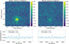 |
Fig. 1 Molecular maps of H2O for real PZ Tel B data using CCS. This figure shows a real case example where the noise structures may reduce detection capabilities of cross-correlation methods. The brown dwarf was observed under good conditions (airmass: 1.11, Seeing start to end: 0.77–0.72) and lower conditions (airmass: 1.12, Seeing: 1.73-1.54), cf. Appendix A for full details on observing conditions. Upper plots show molecular maps of PZ Tel B, while the lower plots show the cross-correlation series along the radial velocity (RV) support for pixels at the centre of the object, and within the object’s brightness area. While the brown dwarf should appear at the same spatial coordinates for respective RV locations in both cases (cf. vertical lines), it is clearly visible when conditions are good, but hardly visible on equal scales under lower conditions. |
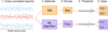 |
Fig. 2 Flowchart representing the methods, scoring, and classification workflows presented across sections. Each cross-correlated spatial pixel (spaxel) is treated as an independent instance and is passed through a classifier of static (statistic) or a dynamic (learning algorithm) type. The methods will evaluate the RV series and yield scoring metrics (e.g. a statistic or probability score). In order to perform classification, the scores need to first be separated using a meaningful threshold. The current standard classification scheme is yield by the S/N on the cross-correlation peak at the planet’s RV. We propose to analyse the RV series in a holistic approach using ML to detect the planets and their molecules, and use the resulting probability scores. |
2 Methodology
This section provides the methodology from the cross-correlation method to the ML algorithms. We start by providing a short preamble, in order to motivate our choice to work with cross-correlated spectra, and to describe the required dataset shape for a spatially independent 1D CNN. Then, we explain the cross-correlation step of a given set of spectra with a molecular template (cf. column 1 from Fig. 2). Subsequently, we present the baselines used to benchmark the performance of our method and the architecture of the CNNs (cf. column 2 from Fig. 2).
Our approach aims to classify spectra individually, based on signature molecules in exoplanet atmospheres. Yet, our previous attempts to classify raw spectra directly with ML algorithms were inconclusive, similarly to Nath-Ranga et al. (2024). However, we found that it is possible to learn a transformation of those spectra, resulting from the CCS method. In fact, Hoeijmakers et al. (2018) emphasise that the CCS has the advantage to co-add the planet’s absorption lines while ignoring the stellar and telluric features. This provided a first level of disentangling of the information in the data, which could be used by a conventional statistic or a learning algorithm. However, to assess a detection, classical metrics like S/N generally rely on Gaussian i.i.d. noise (Ruffio et al. 2019), as well as a strong cross-correlation peak at the planet’s RV. In this regard, we show that the use of neural networks can considerably improve the framework in specific cases of faint signals with unclear crosscorrelation peaks or non-Gaussian i.i.d. noise, as they provide a holistic analysis of the transformed spectra by considering contributions at every RV step. Hence, we employed 1D CNNs to learn molecular signatures in the transformed spectral dimension, thus using the cross-correlation values along RV features. While the cross-correlation step could be integrated into CNNs, we kept this separate to ensure comparable inputs with baselines.
We treated the spectra individually, which allowed the CNNs to train and learn independently from the initial dataset shape and nature. Hence, by doing so, we enabled the MLCCS methods to adapt the training and operate equivalently to long or single slit spectroscopy for different spectral resolutions (e.g., VLT/SINFONI, VLT/SPHERE, GPI, JWST/NIRSpec, CRIRES+, Keck/OSIRIS, Keck/NIRSpec), and generalise to emission or transmission spectra. To achieve such one-dimensional operation, datasets needed reshaping to incorporate spectra as row elements and wavelength bins as columns. To analyse an IFS cube or long slit images, each spaxel (spatial pixel with a wavelength dimension) had to be stacked vertically. Spectroscopic datasets tend to have multiple exposures, introducing a time dimension across wavelength cubes or frames. Our method is designed to perform detection on individual (or sub-combined) exposure units, eliminating the need to combine cubes. Actually, working with uncombined cubes proved to be beneficial for our ML tasks, as it increased the available data while providing a more complex and variable noise structure. It was only crucial to maintain sensible indexing for the spatial and time dimensions to preserve integrity of the training and testing sets, and ensure reliable spatial and temporal reconstruction of the results.
2.1 Cross-correlation of the spectra with the templates
To obtain a dataset of transformed spectra, every spectral element of the dataset was cross-correlated with a template. As variations of chemical composition and atmospheric parameters are large and intrinsic to each planet in a stack of spectra, it would require as many different templates as there are planet variations to obtain exact cross-correlation fits. Thus, the use of full atmospheric templates are useful when searching for one (or a few) particular companion(s) with known properties. However, in practical applications, when searching for unknown and previously undetected candidates, one will not have prior knowledge about spectra which do contain a planet, nor about which template parameters provide the best fit to a candidate planet. Thus, attributing an exact template fit to each spectrum in a large stack without such prior knowledge is unfeasible. Nevertheless, optimal template fit is not necessary for detection. Thus, we could use an imperfectly matching template, that was sensitive enough to weak signals; this was sufficient for detecting the molecule and the associated sub-stellar companion.
In our case, the primary goal is to detect exoplanets by broadly leveraging candidate characteristics. To achieve this, we needed the MLCCS methods to remain as agnostic as possible regarding the chemical composition and atmospheric physics defined in the templates. The aim was to maximise the amount of candidate discoveries across a variety of planets and brown dwarfs, while using a minimal amount of templates and parameters. For instance, using a full chemical composition in an atmospheric template was too restrictive towards any planet which would not match the criterion. Instead, we widened the search by relaxing assumptions on characterisation: we used a single molecule of interest which was generally able to indicate the presence of a substellar companion (e.g. H2O, CO, etc). Following our agnostic approach, we only made very general approximations by selecting arbitrary atmospheric parameters such as effective temperature (Teff) and surface gravity (log g), in a way that roughly covered the parameter space of the class of planets we searched for (e.g., gas giants with detectable amounts of water). Taking this into consideration, we used the template to repeatedly cross-correlate each spectral series (row element) of the dataset. This resulted in a cross-correlated dataset as represented in Fig. 3.
We name the resulting cross-correlated data frame a “template channel”, in lieu of the usual RGB colour channel used for CNNs on standard white light images. Here, each template channel of the same spectral dataset results from its cross-correlation with a different template. If multiple templates are required to incorporate flexibility regarding assumptions on atmospheric characteristics, we use several template channels for the same spectral dataset:
Channel 1 [N × 4001]: (Datasetk * Template 1)
Channel 2 [N × 4001]: (Datasetk * Template 2)
…
Channel M [N × 4001]: (Datasetk * Template M)
where (Datasetk) is a dataset composed ofa stack of spectra from one or several data cubes. N is the total number of spectra in the Datasetk. Thus, if we used M different templates on Datasetk, it results in M different template channels, being cross-correlated variations of the same Datasetk.
The cross-correlation function was applied between the templates and each spectrum of every datasets for 4000 RV steps. A series of cross-correlation values were obtained between RV = [−2000; +2000] km s−1, as the template was Doppler- shifted in steps of 1 km s−1. A cross-correlation peak would be expected to appear at the planet’s RV relative to Earth (e.g., RV = x km s−1), provided the template’s composition matched the spectrum. We adapted the crosscorrRV function from the PyAstronomy library in Python by including a standardisation factor. This resulted in the following equation:
 (1)
(1)
with CCFw,i,m the standardised cross-correlation between a spectrum Sj,i and a template Tj,w,m at RV = w km s−1 (∀w ∈ Z : [−2000, +2000] km s−1). For Si, j, j (∀ j ∈ ℕ : [1, J ]) is the jth element of the spectrum vector in data row i (∀i ∈ ℕ : [1, N]). For Tj,w,m, j is the jth element of the Doppler-shifted and interpolated template spectrum m (∀m ∈ ℕ : [1, M]) at RV = w km s−1. The template spectrum m is one template among a variety of M templates (if multiple need to be used to construct the CNN channels). Every cross-correlation point w is calculated for a template shifted at RV = w km s−1. Thus, CCFi,m is the ith cross correlated vector (row) for template channel m.
There were several advantages of standardising the crosscorrelation, as in Eq. (1). First, the standardised cross-correlation peak could only reach a maximum of 1 in the case of an exact match, which happens when a series is cross-correlated with itself. This standardisation made the peak values comparable between cross-correlated spaxels, allowing interpretation of the signal strength by the ML methods. In addition, normalisation ensured robustness of the classifications against contrast and brightness variations in the image noise, which can affect the absolute cross-correlation peak strength (Briechle & Hanebeck 2001). We note, in this case, that the cross-correlation noise was centered around a mean of 0, which made normalising and standardising equivalent.
 |
Fig. 3 Illustration of the shape and size of one cross-correlated dataframe. Each row is a sample and represents a cross-correlated spaxel (CC spaxel). The RV steps are called features, and the elements of the last column Y are the categorical labelling indicating the presence of a planet or molecule of interest in the spectra. One whole cross-correlated dataframe as above is named a template channel; it results from the cross-correlation of the whole spectral dataset (i.e. all samples) with a unique template. |
2.2 Performance benchmarks
In order to make performance assessments of the MLCCS methods, we defined the S/N as the primary baseline. Moreover, to ensure an informative benchmark for the CNNs, we evaluated the performance of a single layer neural network, called perceptron.
2.2.1 Signal-to-noise ratio statistic
In order to compute the S/N of a cross-correlated series, we followed de Kok et al. (2013) and Petit dit de la Roche et al. (2018). Hence, we evaluated the peak strength at the RV of the planet, namely RV = x km s−1, over a noise interval z in the same series, situated at least ±200 km s−1 away from the peak centre x:
 (2)
(2)
where CCFx,i,m is the cross-correlation value at x km s−1, (∀X ∈ ℤ), for an empirical standardised cross-correlation vector (∀i ∈ ℕ : [1, N]) between spectra of planets inserted in noise and a template channel m (∀m ∈ ℕ : [1, M]). We note that x = 0 km s−1 for a companion at rest frame. CCFz,i,m represents the series of noise values taken ±δ km s−1 away from the cross-correlation peak. The interval of [x − δ; x + δ] km s−1 corresponds to the point where the strong signals generally appear to fade out and the cross-correlation wings mimic randomness (cf. Fig. 1). Thus, for H2O, we would have z ∈ ℤ : [−2000; 2000] \ [x − 200; x + 200] km s−1 for the same cross-correlation vector series i, in the same template channel m.
By construction, a fundamental assumption of the S/N metric is the Gaussian i.i.d. behaviour of residual cross-correlation noise (whether taken from cross-correlation wings or any other spaxel in an image), inherited by the assumed Gaussianity of the spectral noise. However, we highlight two reasons for the disputable nature of the commonly accepted detection thresholds and their resulting confidence intervals, namely for T = 3 for 3σ and T = 5 for 5σ detections.
Primarily, inconsistencies in S/N computation across the literature (cf. Sect. 1) and in the choice of intervals impact the interpretation of detection thresholds and confidence intervals. Under the (asymptotic) Gaussian noise assumption, a Z-statistic (or respectively t-statistic) incorporating a proper variancestabilising factor are more reliable. Therefore, we emphasise that we have also tested the methods against alternative S/N measures, that is, using the noise from a different spaxel as in Hoeijmakers et al. (2018); Patapis et al. (2022), correcting the cross-correlation for template auto-correlation as in Cugno et al. (2021); Patapis et al. (2022), or even using a proper t-test statistic. As the scores of those tests did not affect the results and conclusions of this study, they are left out of the paper for the sake of readability.
Secondly, spectral noise tends to be non-Gaussian or at least non-i.i.d. due to various noise sources and their effects on the cross-correlation (cf. Sect. 1). While cross-correlation noise is optimal and equivalent to maximum likelihood estimator under well-behaved spectral noise (Ruffio et al. 2019; Brogi & Line 2019), non-Gaussian i.i.d. spectral noise causes cross-correlation to be sub-optimal. Fortunately, neural networks don’t rely on Gaussian or i.i.d. assumptions to yield correct classifications, thereby offering an alternative approach to improving detection performance in the presence of complex spectral noise.
2.2.2 The perceptron as an MLCCS baseline
The perceptron is a simple linear neural network with no hidden layer, and only one activation function. In our case, it contains only the sigmoid activation function, which makes it similar to a logistic regression. Hence, it is the simplest form of a binary neural network classifier. We used this simple architecture, shown in Fig. 4, as a baseline performance to track improvements of more complex and non-linear neural networks such as the CNNs, presented in Sect. 2.3.
The perceptron takes a stack of cross-correlated spectra as input, and outputs a vector of probabilities, relating to the presence of a molecule of interest in each spectrum (cf. Fig. 2). The algorithm learns the patterns linking features of the input data to the label according to a training set. In order to learn the task, it was given a portion of the input dataset as training set, together with binary labels informing about the presence or absence of a molecule of interest in each cross-correlation vector series. We performed an iterative search process, varying the hyperparameter set, to evaluate which perceptron model trained best on a validation set. This hyperparameter search process was done using a meta-heuristic algorithm. Once the best model was found, it was evaluated on a test set, which was reserved as a last portion of data for model evaluation. All those steps were applied in a cross-validated fashion to investigate the stability of the test results across different portions of a dataset. Further details on the splitting of our mock datasets for training, validation and testing are described in Sects. 4.1 and 4.2.
The perceptron was developed and trained using the keras library in python (Chollet 2015; Gulli & Pal 2017). We included early stopping, which is similar to low L2 type regularisation on the RV features. The model’s solution on the log-loss term was found with the RMSprop1 optimiser. As for the hyperparameters, they were optimised by a heuristic evolutionary algorithm. Thus, for every new dataset, we set prior bounds on hyperparameters listed below and let the process converge:
Batch size: This hyperparameter regulates the trade-off between the training speed and the accuracy of the gradient estimates. We allowed for five possible values from the set: Bsize = {16, 32,64,128,256}.
Epochs: Optimising for the number of epochs corresponds to an “early stopping” regularisation of an L2 type. We let the network learn over a continuous range of possible values: E = [100,200] with E ∈ N.
 |
Fig. 4 Architecture of the perceptron. This simple one-layer neural network analyses the values of a whole cross-correlation series in a holistic approach to detect the presence of a molecular signal. |
2.3 Convolutional neural networks
Convolutional neural networks (Krizhevsky et al. 2012; O’Shea & Nash 2015; Gu et al. 2018) are a class of models which have proven to achieve formidable results in pattern recognition tasks. In their two-dimensional form, they are typically used for image recognition and classification, as they are robust to small pattern shifts and variations in space. In our framework, we applied 1D CNNs (Malek et al. 2018) on the RV dimension of the samples.
While a S/N statistic is only able to evaluate a spectrum based on a single given point (i.e. the cross-correlation peak), ML algorithms are able to take a holistic evaluation of patterns by considering all RV features in each cross-correlation series. However, what makes the CNNs important for our case are the benefits towards uncertainties of exoplanet atmospheric compositions. While the S/N and the perceptron can only be given one template channel at a time, the CNNs are able to use multiple template channels simultaneously, presenting different atmospheric properties. This means that we could consider several cross-correlated variations for one spectrum, as shown in Fig. 5. This enabled uncertainties regarding atmospheric characteristics to be incorporated when searching for previously uncharacterised planets. In fact, the number of template channels were used as filter depth for the CNN (cf.cf. Fig. 5). Then, the CNN uses convolution and pooling layers to downsample those channels. This allows one to reduce the matrices and extract important patterns efficiently. The two CNNs we used are presented below.
2.3.1 Convolutional neural network architecture
Our main model (CNN1), as shown in Fig. 6, is made of convolutional and pooling layers, followed by one final dense layer which is similar to the perceptron. With this network, we could test and isolate the effect of adding convolutional layers in comparison to the perceptron. Thus, CNN1 does not include any other regularisation than the early stopping criterion (similar to L2). We emphasise that regularisation and increased model depth can come at the expense of invariance of a CNN to pattern shifts (such as RV shifts of the planet in the cross-correlation), which provided the motivation to keep the model simple. To train and optimise the CNN, we used the stochastic gradient descent, with Nesterov momentum and an optimised learning rate, we set the hyperparameter bounds to the following:
Batch size: we let the optimiser choose among three possible values from the set: Bsize = {16,32,64}.
Epochs: we let the network learn over a range of possible values: Epoch = [100,200] with Epoch ∈ ℕ.
Learning rate: the bounds of the learning rate of the stochastic gradient descent are set to η = [0.0001,0.01].
Momentum: the bounds for the momentum are widely set such that Mom = [0.1,0.9].
Kernel size: this hyperparameter regulates the size of the convolutional filter. The Kernel size is set as one same parameter being valid for both convolutional layers. The set is configured to be integers in Ksize = {3,5,7}.
Max-pooling: the maximum pooling take the maximum value over ranges of values of the convolutional layer’s output, and pools them together. The maxpool parameters are defined as integers over the set Pmax = {2,3}.
2.3.2 Testing regularisation schemes in dense layers
Ultimately, we tested a CNN with a regularisation structure (CNN2) to verify if the general CNN framework needs regular- isation or if overfitting is sufficiently controlled by our training scheme. Regularisation allows one to reduce the unwanted complexity of a model and thus overfitting by, for example, dropping some features (drop-out) or by rescaling the weights of the features to a maximal L2 norm. The CNN2 includes two convolutional and max-pooling layers as well as three dense layers that use Leaky-ReLu activation functions. We combined several L1 and L2 regularisation types on the dense layers. We added two drop-out layers with individually tuned drop-out rates combined with one kernel constraint on the activation of the last hidden layer. The final neurons were mapped into the probabilistic prediction space by a sigmoid function. The detailed architecture is presented in Fig. 7. The model was optimised with stochastic gradient descent; we set the following bounds for the meta-heuristic optimiser:
Batch size: we let the optimiser search over the set Bsize = {16,32,64}.
Epochs: we let the network learn over a range of possible epoch values to define the equivalent of an early stopping rule such that Epoch = [100, 200] with Epoch ∈ ℕ.
Learning rate: the bounds of the learning rate of the stochastic gradient descent are set as η = [0.0001,0.01].
Momentum: the momentum’s bounds are Mom = [0.1,0.9].
Kernel size: the set of kernel sizes is defined once for both convolutional layers as Ksize = {3,5,7}.
Max-pooling: the parameter of both maximum pooling layers are defined once as integers over the set Pmax = {2,3}.
Leaky ReLu: in the case of the convolutional neural network, due to the high amount of tuning hyperparameters, we set the same bound for any Leaky ReLu activation as α = [0.1,0.9]
Drop-out: in this convolutional neural network, we have defined two layers of L1 shrinkage, for which two hyperparameters were set so that the bounds are the same for D1 = [0.1,0.8] and D2 = [0.1,0.8].
Kernel Maxnorm: the Kernel maximum norm, equivalent to the L2 regularisation, were set to be Kmax = [0.1,5].
Finally, each ML method was trained and tested on two datasets that were fed to the algorithms as a stack of cross-correlated series. The construction of both datasets is described in Sect. 3. For each of the MLCCS models, the hyperparameter tuning was automated using an evolutionary algorithm that performs a heuristic search over the hyperparameter space. The benefit of using this training scheme is that it provides high stability on the results. All models were trained and tested in a cross-validated fashion, with folds delimited by the temporal cubes. The algorithms predict a probability score for a molecular feature to be present. Hence, in order to separate the groups between signals and noise, we had to define a meaningful threshold. Regarding the preservation of clarity and readability, we discuss this last step in Sect. 4).
 |
Fig. 5 Example of the application of a CNN on one cross-correlated spectrum. For each sample of a cross-correlation N, and for all M template channels, the convolution filter runs across the channels and along the RV series. The filter depth is M, and its size is optimised according to the training. Hence, for a same series cross-correlated with M different templates, those convolutional layers allow to filter out important and recurrent patterns. |
 |
Fig. 6 Architecture of CNN1. This figure illustrates the architecture of our CNN with several convolution layers and one dense layer. This model tests the effect of adding convolutional layers and template channels in addition to the sigmoid activation. |
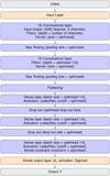 |
Fig. 7 Architecture of CNN2. This figure illustrates the architecture of our second CNN. It includes regularised layers to evaluate the benefit of regularisation for generalisation to different target noise regimes. |
3 Data
In order to show that the MLCCS approach is flexible across planet types and instruments, we validated this proof of concept on two datasets described in this section. The first dataset is called the ‘extracted spectra of companions’, and it represents a stack of individual spectra. Those spectra contain random insertions of synthetic gas giants and brown dwarfs among real instrumental noise. The purpose is to evaluate the capacity of the MLCCS methods to learn effective detection and classification on isolated spectra, for various planet types (e.g. for stacks of spectra without a relevant spatial structure). The second dataset is the ‘directly imaged companions’ dataset, and it evaluates the model’s capacities to operate on unbalanced datasets where signals are scarce. It also investigates capacities to detect faint sub-stellar companions in structured data such as imaging spectroscopy.
Both datasets were built out of a common basis of simulated planets embedded in real non-Gaussian i.i.d. noise. While the spectra of the synthetic planets were simulated using petitRADTRANs Mollière et al. (2019), we gathered the instrumental noise using spaxels from noisy areas of real observations. Those were from GQ Lup B and PZ Tel B, observed in K-band at medium resolution R ~ 5000 using SINFONI, the near-infrared spectrograph mounted on the Very Large Telescope (VLT). The data preparation steps are thoroughly described, as they are the determinant for quality and reproducibility of the results. We first outline the three steps which build the common basis for both datasets, namely, the IFS noise extraction, and the simulation of the planetary signals and molecular templates. Then, we explain how the synthetic planets were inserted into the extracted spectra of companions and the directly imaged companions datasets, and how these were prepared for the tests.
3.1 Preparation of instrumental noise cubes
The results of this proof of concept rely on the calibration and quality of the datasets and noise. In fact, ground-based spectral imaging noise can be non-identically distributed and non-independent (non i.i.d.) up to non-Gaussian, due to instrumental, telluric, stellar effects, and therefore difficult to simulate faithfully. The use of simplistic simulated i.i.d. Gaussian noise will lead to an inaccurate prediction of the performance of the ML methods, thus preventing reliable generalisation to real non-Gaussian noise. Therefore, it was preferable to use real preprocessed VLT/SINFONI noise to guarantee accurate evaluation of the MLCCS methods. In this regard, we extracted noise from a total of 19 uncombined integral field unit (IFU) cubes from GQ Lup B and PZ Tel B observations in K-band medium resolution spectroscopy, presented in Table 1.
Following Cugno et al. (2021), the raw GQ Lup B and PZ Tel B datasets were first reduced with the EsoReflex pipeline forthe SINFONI instrument (Abuter et al. 2006), which includes steps such as dark subtraction, bad pixel removal, detector linearity correction and wavelength calibration. It outputs 3D data cubes for each science observation. Hence, each science cube consists of two spatial dimensions and a wavelength dimension covering 1.929–2.472 µm. As NaN values were located at the waveband edges, the latter were removed by trimming the cubes to a wavelength dimension spanning from 1.97-2.45 µm for GQ Lup B and 2.00–2.44 µm for both PZ Tel B datasets. Finally, a customised version of the PynPoint pipeline(Amara & Quanz 2012; Stolker et al. 2019) was used to remove the stellar contribution (and the companion pseudo-continuum) from the frames. This step was performed applying high-resolution spectral differential imaging (HRSDI, Hoeijmakers et al. 2018; Haffert et al. 2019); we modelled and subtracted the low-frequency spectral component in the data in order to leave only the high frequency components from the molecules in the planet’s atmosphere. A detailed description of data preprocessing can be found in Cugno et al. (2021). The resulting wavelength cubes were not mean or median combined in time for two reasons. First, we wanted to preserve a rough noise structure to ensure the robustness of the ML algorithm to variations in noise. Second, it also allowed one to use enough original data to train the ML algorithms without having to use data augmentation techniques, which could have increased risks of overfitting the data.
Before flattening of the 19 pre-processed IFU cubes into a stack of spectra, the spaxels containing the true companion’s signal were identified in each residual wavelength solution, using target centring coordinates. The signals were then confirmed using cross-correlation with a template. A wide aperture (radius of 5.5 pixels) was drawn around the target’s centre, such that the spaxels containing the true planets were removed from every cube with an additional margin of minimum two pixels. This was done to ensure an accurate and unbiased labelling of the training, validation and test sets, and avoid leakage of real molecular signal from the targets companions into the noise. After removal of the companions, the cubes were flattened and stacked, such that the noise spaxels from each and every cube were stacked along a unique spatial dimension to form an instrumental noise basis that we could sample from.
IFU cubes used for noise extraction.
3.2 Simulated planets and molecular templates
In this section, we describe the simulation of the templates and the planets that were inserted in the real noise spaxels. The synthetic companion spectra were simulated with petitRADTRANs (Mollière et al. 2019), as simplified gas giant and brown dwarf atmospheres. Their composition was made of molecules of interest such as water, carbon monoxide, methane, and/or ammonia molecules (H2O, CO, CH4, NH3), with a hydrogen and helium dominated atmosphere. Overall, ten possible singleton or pairs of molecules of interest were included in the atmospheres in addition to the hydrogen and helium rich environment. Realistic molecular abundance profiles were defined along the vertical extent according to the chemical equilibrium model yield by easycHEM (Mollière et al. 2017).
As for the atmosphere’s structure, the radiative transfer routine petitRADTRANs relies on a parallel-plane approximation, and the simulations were made under the assumption of 100 layers atmospheres, between 102 and 10−6 bar (equally distant in log space). The Guillot model was used to parameterise the P-T profiles (Guillot 2010). This model assumes a double grey atmosphere with a characteristic opacity in the optical (κVIS) and in the thermal (κIR), thereby decoupling the incoming stellar irradiation from the outgoing planetary flux. The following values of γ = κVIS/κIR = 0.4, κIR = 0.01 cm2 g−1, and interior temperature Tint = 200 K were used. The surface gravity and equilibrium temperature (translated into effective temperature) are the two last parameters of the Guillot model. Those were varied to create the planets grid, as log ɡ and Teff may affect the spectral lines via the thermal structure and vertical mixing. Following Stolker et al. (2021) and Hoeijmakers et al. (2018), the planets were simulated on a grid of Teff ranging from 1200 K to 3500 K with steps of 10 K, and log g ranging from 2.5 to 5.5 dex, with steps of 0.2 dex. In this setting, the metallicity and C/O ratio were kept fixed to solar values (Fe/H = 0.0 and C/O = 0.55). Overall, for each combination, we obtained a grid of 231 Teff and 16 log ɡ values, thus 3696 synthetic planet spectra per molecular combination and 36 960 spectra over all combinations. Finally, the continuum was approximated and removed using a Gaussian filter; a window size of 60 wavelength bins (15 nm) allowed for effective removal of the continuum without leaving any measurable trends or bumps in the residuals.
As for the molecular templates, high resolution emission spectra of H2O were generated with petitRADTRANs, using thermal structure grids. While the P-T profile model is the same as defined above, the molecular abundance of water was set to a constant −2.0 dex (i.e. mass fraction = 10−2) along the vertical extent of the atmosphere to produce well defined absorption lines. Then, the template was downsampled to the spectral resolution of the data and the same Gaussian filter was applied on the spectra to subtract the continuum emission.
A selection of the single molecular templates was cross-correlated with each mock dataset outlined in the upcoming sub-sections; this returned several template channels per set, which we used to feed the CNNs. Since the focus is set on detection of new candidates rather than precise characterisation, we have to assume that the characteristics of the synthetic planets are unknown. Thus, we need to make minimal assumptions to maximise the number of detections. This means that it is preferable to use several template channels to vary the atmospheric characteristics. We did not identify a hard rule on the number of template channels for the CNNs, and those can be chosen relatively arbitrarily. Nevertheless, through our tests, we observed general trends helping the CNNs perform well. First, expanding or refining the template channel grid has a benefit to cost trade-off between gaining in flexibility to find more planets from adding templates, and computational complexity. In addition, the marginal benefits in agnosticity from adding one template will start to culminate. The best benefit to cost we noticed was between five and ten template channels. Second, we did not identify any consistent or clear change in performance by changing templates. Still, the template parameters should be roughly spread over the parameter space of interest. Overall, those rules of thumb will depend on the dataset’s characteristics, for instance its size, the variability of the planets it contains, or the available computational resources. As for the selection of the molecular composition, the most agnostic approach is to use a parallel combination of single molecular templates to detect planets that have at least one of the stated molecules. Alternatively, one can use one molecule for all templates to apply a weaker constraint on composition.
For the proof of concept, we focused on the search for planets with water features by using H2O templates. Primarily, because water is a detectable spectral feature at K-band using CCS, and focusing the detection on a single molecule at a time makes it easier to evaluate the CNNs against benchmarks. Secondly, gas giants and brown dwarfs can be very rich in H2O depending on the location of their formation with respect to the snowlines and separation from the host star (Öberg et al. 2011; Morley et al. 2014; Nixon & Madhusudhan 2021). Thus, water rich planets are relatively abundant in this population and hence convenient for broad search of such exoplanets. Finally, beyond the gas giant framework, it is also of high scientific interest to improve sensitivity to weak water features on smaller sub-Neptune and terrestrial planets in the habitable zone (Madhusudhan et al. 2021; Pham & Kaltenegger 2022). However, we show in Appendix B that the method can as well be trained using templates of single molecules, or combinations of those to find even more planets.
3.3 Mock data of the extracted spectra of companions
Within this section, we present the first mock data, which is named the extracted spectra of companions dataset, as it contains various types of planetary spectra embedded in instrumental noise. The goal of this dataset is to demonstrate the capacity of the MLCCS methods to improve planet detections via water signals while using a minimal amount of prior information. It also proves the ability of the MLCCS approach to operate only in the RV dimension by treating the spaxels independently, i.e. without using any spatial information. Consequently, this one dimensional approach aims to prove the capacity of the MLCCS methods to operate on isolated spectra as well as in various spec-troscopic modes, such as single and long slit spectroscopy (e.g. CRIRES+, Keck/OSIRIS, Keck/NIRSpec). Implementation of MLCCS methods could in principle be adapted to high resolution transmission spectroscopy by generalising the framework.
As explained in Sect. 3.2, we focused the search on water features, which makes H2O the planetary signal of interest; the rest was regarded as noise. The planets were randomly sampled without replacement, and an atmospheric variant could appear only once in the dataset. As a result, over a total of 24 312 spectral instances, 50% of the dataset contains water-rich planets (the ‘positive group’), and encompasses simulated planets composed of combinations of molecules including water. The remaining 50% represents noise (the ‘negative group’). Among the noise, 50% of the spaxels are ‘pure noise’, that is, plain instrumental noise without any molecular spectrum. The other 50% of the negative group is ‘molecular noise’, that is, any planets with combinations of molecules that do not include water to represent water depleted planets.
The instrumental noise was also randomly sampled without replacement from the eight GQ Lup B cubes (see Sect. 3.1). After preprocessing and removal of the real target as described in Sect. 3.1, each cube was left with 3 039 spaxels, yielding a total of 24 312 spaxels. To avoid creating spatial dependencies when training the MLCCS methods, the spaxels within each cube were shuffled to spatially decorrelate the noise. The shuffling was only applied within, but not across the cubes. This allowed us to split our data into training, validation, and testing cube groups without overntting the noise.
Inserting the planets in the noise without re-scaling would have yielded either signals too faint to be detected or very strong signals, leading to perfect classification. For feasibility of the study and comparability of the methods, all planets were inserted at rest frame with a radial velocity of RV = 0 km s−1. The noise was adjusted with respect to the signal, for a scaling factor α:
 (3)
(3)
where S represents the spectral series that is composed of the spectrum of a simulated companion atmosphere (P), and the instrumental noise series (є). We note that the scale factor corresponds to varying the average S/N and hence the average noise level, which encompass both variations in contrast and separation. As the planets were inserted randomly, it is not possible to match a specific scale factor to a contrast or separation for every case. The scale factor can be understood as a random variation of those two parameters, which is in line with our agnostic approach. However, specific tests on the influence of planet separation and contrast for a close category of CNN methods can be found in the companion paper (Nath-Ranga et al. 2024).
Finally, we sampled random templates of water in a cluster design, over values of log 𝑔 = {2.9; 3.5; 4.1; 4.7; 5.3} dex and Teff = {1200; 1600; 2000; 2400; 2800} K. We cross-correlated the dataset into nine cross-correlated template channels, which took about 30s per channel when distributed over 32 CPUs. Fig. 8 sets an example of four randomly picked cross-correlated spectra resulting from the final stacks. It is obvious that no cross-correlation peak is visible at the radial velocity of the planet for the positive group. Hence, separating and classifying each group is non-trivial for a S/N statistic.
3.4 Mock data of the directly imaged companions
This section describes the directly imaged companions dataset, which was used to test and demonstrate that the spatially independent MLCCS methods can operate on structured data such as direct imaging, although it is highly imbalanced. The synthetic brown dwarf spectra were selected from the pool of simulated companions (Sect. 3.2) according to GQLupB and PZ Tel B’s respective characteristics. They were inserted as faint Gaussian ellipses into the respective instrumental noise cubes. The spectra of each of the planets were selected with ranges of Teff = {2450; 2760} K in steps of 10 K and log 𝑔 = {3.7; 4.7} dex in steps of 0.2 dex for the simulated GQ Lup B (after characteristics reported by e.g. Seifahrt et al. 2007; Stolker et al. 2021) and ranges of Teff = {2900; 3100} K in steps of 10K and log 𝑔 = {3.7; 4.7} dex in steps of 0.2 dex for the simulated PZ Tel B (cf. Jenkins et al. 2012). All spectra were selected with a hydrogen and helium dominated atmosphere and composition variations of H2O and CO.
The synthetic planets were inserted as aperture delimited Gaussian ellipses in the cubes, using a subset of selected spectra. Sampling subsets instead of a single spectrum allows for the inclusion of signal variations within the aperture. This ensures robustness and avoids overfitting as the network encounters slight variations of spectra amid noise, it learns to handle encounters of new spectra in realistic test sets. Spectra subsets were sampled without replacement, ensuring that each cube presents a unique planet in terms of atmospheric structure and composition. The planets were inserted as Gaussian ellipses with random variations of elliptic ratio, size, luminosity decay, and locations, as shown in Fig. 9. This specifically prevents the neural networks from learning such deterministic dataset artefacts. This injection approach deviates from the point spread function (PSF) shape and size of SINFONI data, but it enables objective testing of the ML methods’ capability to recognise signals regardless of PSFs and data structure. This is crucial for versatility and generalisability to other spectrographs and instruments while maintaining spatial independence.
We inserted faint simulated companions with H2O (mainly in the brown dwarf regime) at rest frame with an average S/N below the usual detection threshold of 5. The goal was to show that the MLCCS methods could recover such embedded objects, even with a less conservative threshold. Finally, we cross-correlated our dataset according to Eq. (1), for a small grid of templates of water, spanning across several log 𝑔 and Teff values, and roughly covering the parameter space of the inserted companions. We note that the cross-correlation of the whole dataset of 57 782 spectra with 1436 wavelength bins into one template channel took about two minutes when allowing for distribution over 32 CPUs. This was performed for five template channels for each dataset, respectively with Teff = {2700; 2800; 2900; 3000; 3100} K and log 𝑔 = {3.7;4.1;4.1;4.3;4.1} dex, and a total of 17 cubes to train on. The two remaining cubes were kept for validation and testing.
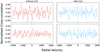 |
Fig. 8 Four randomly selected cross-correlated spectra from the final extracted spectra of companions dataset. For this particular case, the signals were inserted at RV = 0 (dashed vertical line) with a scale factor of eight, which corresponds to an average S/N of ≃0.633. This plot aims to show how the transformed spectra with H2O signals (blue) do not show a visible cross-correlation peak, nor any obvious patterns that differ from the negative group (red); separating the groups based on a S/N statistic is non-trivial. |
4 Results and discussion
In this section, we describe the metrics used to evaluate the models. Then, we present the results from those metrics on each dataset, and put the results in perspective with a sensitivity analysis. Finally, we discuss the implications of this work for the community, and propose further research.
After passing the cross-correlated stack through the ML algorithms, the trained models assign an output score to each instance, which represents the probability of a spectrum to belong to the positive group (i.e. spectra with water). We used the extracted spectra of companions dataset to quantify how many of the inserted planets could be found despite the diversity of their spectra. Then, we verified the capability of those spatially independent methods to perform on structured data, such as the directly imaged companions mock data. To do so, we evaluated the quality of the scoring against benchmarks, and quantified the resulting predictions. In order to divide the spectra into two predictive groups, namely the positive (exoplanets with H2O) and negative groups (no H2O detected), we needed to separate the scores by using a threshold that yielded predicted classes. We could then evaluate those predictions according to elements of the confusion matrix (see e.g. Jensen-Clem et al. 2017), which included the amount of correct detections (TP), of false detections (FP), of missed detections (FN), and of correctly discarded spectra (TN).
To formalise this, we used receiver operating characteristic (ROC) curves (Fawcett 2006) to show the performance on the balanced dataset (i.e. the extracted spectra of companions). This evaluation metric allowed us to explore the trade-off between correctly detecting exoplanets and incorrectly selecting false positives. As we would vary either the classification threshold along the scores or some of the model tuning parameters, we could increase the true positive fraction, but would have to bear the cost of simultaneously increasing the false positives by a certain fraction (i.e. we would simply be travelling along the curve). However, by using a better model, we would take a stride to a higher curve. Hence, measuring the area under the ROC curves (ROC AUC) generally allows for evaluation of the overall gain over the trade-off in statistical sensitivity (or true positive rate, or TPR) relative to the false positive rate (FPR), which are defined in Eqs. (4) and (5) as follows:
 (4)
(4)

Although ROC curves are very useful to evaluate the scoring quality on balanced datasets, they tend to show over-optimistic results on imbalanced datasets. Therefore, when evaluating our methods on imbalanced data (e.g. full images), we considered an additional trade-off measure, namely the precision-recall (PR) curve. The recall corresponds to the true positive rate in Eq. (4), and is evaluated against precision, which is known as the positive predictive value or the true discovery rate (TDR), as described in Eq. (6):
 (6)
(6)
The precision-recall measure is more sensitive to improvements in the positive class and true detections (Davis & Goadrich 2006), and is used to evaluate cases where the data is highly imbalanced (Saito & Rehmsmeier 2015), such as our directly imaged companions data.
Finally, to evaluate the results in the light of a meaningful classification threshold, we introduced the false discovery rate (FDR, Benjamini & Hochberg 1995), which is another existing metric that has been employed (for example in Cantalloube et al. 2020):
 (7)
(7)
This metric is very meaningful for data analysis of surveys or archives, since it is able to control the impurity of the predicted positive sample, i.e. the proportion of false positive leakage into the claimed detections, as shown in Eq. (7). We emphasise here the difference with the false positive rate, which only controls for the amount of false positives leaking from the true negative population. Hence, the ROC curves and FDR metrics presented above will be used to evaluate the detection performance of the MLCCS methods against the S/N on the extracted spectra of companions.
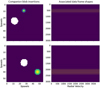 |
Fig. 9 Spatial decorrelation in two IFU cubes of the structured mock dataset for directly imaged companions. Left panels: brown dwarf signals inserted in a structured manner, as varying Gaussian decaying ellipses within a delimited aperture, showing variations in position, size, and shape. The white areas indicate removal of real companions. Right panels: plots illustrating datasets after flattening and transformation, with the horizontal axis representing radial velocity and the vertical axis representing stacked spatial dimensions. Visible lines denote spax-els with inserted planetary signals, showing variations based on the inserted planets’ properties. This method prevents the ML algorithm from learning redundant spatial artefacts; it emphasises learning from cross-correlation patterns in the spaxel dimension. |
4.1 Results of the extracted spectra of companions dataset
Through those results, we evaluate the effectiveness of the MLCCS methods in finding water rich planets in the extracted spectra of companions dataset. This test aims to demonstrate the MLCCS methods’ ability to detect a variety of planets embedded in genuine instrumental noise. Thus, the main results are presented according to planet insertions that return extremely faint H2O signals in the positive group with an average of S/N ≃0.633, against S/N≃0.044 for the negative group (cf. Fig. 10, top panel). Moreover, the CNNs take nine channels as input, which relate to various templates of water spanning over combinations of Teff = {1200; 1600; 2000; 2400; 2800} K and log 𝑔 = {2.9,3.5,4.7,5.3} dex (see Sect. 3.2). We note, that the S/N and perceptron baselines can only take a unique data template channel. The channel we used is issued from a template of Teff = 1200 K and log 𝑔 = 4.1 dex. We also ran a sensitivity analysis, by assigning different template channels to the baselines; the results did not show any significant difference in the performance evaluations, and are therefore left out of the study.
The models were trained along the temporal dimension, specifically on six exposure cubes, then validated on one cube and tested on a remaining one. The training and testing routines were performed in a parallelised cross-validated fashion, with each fold running on its own GPU. The hyperparame-ter search process was automatised and took about four hours end-to-end for one CNN (on a NVIDIA GeForce RTX 2080 Ti GPU). This provided stable results across folds and allowed us to get around lengthy hyperparameter fine-tuning, which would be difficult for users with limited experience with ML algorithms. However, runtime will vary according to the dataset size, number of channels, hyper-parameter search, and available computational resources. We show the aggregated ROC curves over all tested cubes in Fig. 11. It shows the drastic improvements of the MLCCS methods in terms of scoring quality, with AUCs of 0.884 and of 0.871 for CNNs, and 0.792 for the perceptron, against 0.653 for the S/N metrics, for a given scale factor of α = 8. This means that, for the same FPR, the CNNs could raise more true candidates. The scoring quality improvements can be explained by observing the frequency distributions on the aggregated scores over all tested cubes, as shown in both upper panels of Fig. 10. The scores assigned to the data by a classifier can be understood as the likelihood of a given spectrum to actually belong to the group of planets with water, according to the classifier. The CNN exhibits high scoring confidence in distinguishing between the two groups, which translates into a strong contrast in scores’ distributions. To avoid confusion with the usual meaning of contrast in astronomy (i.e. brightness of a planet relative to its host star), we favour the word “conspicu-ity”. This effect makes the CNNs effective in detecting planets with water in the dataset and simultaneously reducing the occurrence of false positives. On the contrary, the S/N statistic scores show a poor conspicuity between both groups, forcing the use of high confidence thresholds (e.g. T = 5), involving conservative results with higher FNs.
To quantify classifications, we set thresholds to be comparable across scoring measures, aligning with a maximal FDR of 0.05 (Fig. 10). We chose this value according to conservative standards in the field of statistics (Benjamini & Hochberg 1995), but it is of course possible to choose a more conservative value. The threshold should be adjusted for a desired confidence level before it can be used to evaluate detection performance of the models. Thus, the lower panel in Fig. 10 illustrates the maximum achievable detections when bounding false positives up to 5% of the predicted detections. While S/N detects 88 true planets, the perceptron finds 26 times more with 2 318 true detections. This renders a sensitivity (TPR) of 19.3%, against 0.7% for the S/N. We note that the detection purity (TDR) always remains comparable, with 95.0% for the perceptron against 95.6% for the S/N, due to the upper bound on the FDR. However, a key aspect of our methods is our presumption that precise knowledge of a planet’s characteristics is not necessary for detection. This aspect is strongly connected to the significant improvements observed in those results. Indeed, even the use of a single molecular template with the perceptron enabled the detection of hundreds of planets. This happens as we focued on finding weak signals rather than searching for strongest peaks that would only occur for highly matching templates. Yet, the extra leap in detection sensitivity is offered by the CNNs, with the incorporation of multiple template channels as filters, which provided flexibility regarding composition uncertainties. In fact, the CNNs are capable of casting a wide net to discover more planets despite variations in atmospheric characteristics, thanks to the agnostic approach. Thus, each CNN achieves over 6000 real detections out of 12000 inserted planets (Fig. 10), representing a statistical sensitivity of 51.2 and 55.5% TPR respectively, with a purity of 95.0% TDR. In other words, this test has proven that MLCCS can diversify planet searches in a single attempt, irrespective of the data structure.
The results of this section were presented according to a scale factor of α = 8, which yields very strong noise with regard to signals. Yet we note that the efficacy of MLCCS methods is negatively related to noise levels at the extremes, as illustrated in Fig. B.1. If α is excessively small or large, the improvements over S/N metrics become marginal. For completeness of the study we discuss the interpretability of the results in the light of a sensitivity analysis over a range of scaling factors α in Appendix B.1. In addition, we also provide extended tests and discussion on the flexibility of MLCCS towards exoplanet compositions by incorporating variations of molecules in the template channels (cf. Appendix B.2). We also provide an explainable framework by verifying that MLCCS is able to learn patterns in non-Gaussian noise (cf. Appendix B.3) and molecular harmonics (cf. Appendix B.4). Finally, we prove in Appendix B.5 that MLCCS methods are generally robust and consistent in detecting planets despite small changes in the cross-correlation length and extent, and that CNN1 is able to achieve invariance to RV shifts of the planet in the series.
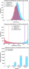 |
Fig. 10 Scoring and classification of the S/N and CNN. Top and middle: frequency distributions of aggregated scores assigned to the negative group (red) against the positive group (blue) for both methods. The scores represent the predicted likelihood of a given spectrum to belong to the positive group. The probabilistic scores assigned by the CNN provide a better separation of the groups (i.e. “conspicuity”) than S/N scores. Classification predictions are set by a threshold for a FDR at 5%. Lower: maximal amount of planets recovered in the mock data by the S/N, perceptron (PCT) and both CNNs, within a maximal FDR of 5%. |
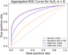 |
Fig. 11 Quantification of scoring performance with ROC curves. The plot shows the improvements in the ROC trade-off between TPR and FPR. The improvement is measured in terms of area under the ROC curves (AUC). The CNNs outperform the baselines in finding true positives while limiting the increase in FPR. |
4.2 Results of the directly imaged companions dataset
In real-world scenarios, datasets are often highly imbalanced due to various reasons, such as the limited number of planets found in surveys, or the small fraction of spaxels containing a planet in a full image. Consequently, the directly imaged companions dataset (cf. Sect. 3.4) serves a dual purpose. Not only it demonstrates the ability of MLCCS to recover a planet in imaging data without relying on spatial information, but also shows its broader effectiveness in handling highly imbalanced data. We prove the general capacity of MLCCS on structured and reconstructed cubes, and hence presents global performance results for given noise levels (may it be stellar, instrumental or telluric). For a high contrast imaging oriented analysis measuring achievable ML performances regarding different contrast and separations, we refer to our paper companion Nath-Ranga et al. (2024). They apply multi-dimensional CNNs specifically for high contrast imaging spectroscopy and show results for a set of contrast and separations.
The models underwent training and validation on individual cross-correlated spaxels from 18 cubes and were tested on the last cube in a cross-validated fashion of three tests. The end-to-end automated hyperparameter search process took about seven hours for a CNN. The baseline methods employed a single template channel (Teff = 2900 K, log g = 4.1 dex), while the CNNs used four channels simultaneously (Teff = {2300,2500,2700,2900} K, log 𝑔 = 4.1 dex). Figure 12 shows the scoring improvements performed by the MLCCS methods in comparison to the S/N metric, in terms of aggregated ROC and PR AuCs. For one image, the amount of positives (i.e. spaxels containing a planet in the image) are of the order of ~1% making it a highly imbalanced regime. The ROC curves are shown to enable comparison with plots related to the extracted spectra of companions. Nevertheless, for quantification of the results, one should rely on the P-R Curves. While the PR AuC of the S/N equals 29.5%, the AuC of CNN1 achieves up to 57.7%, which represents a very big improvement for such imbalanced data. Results per test cubes are visible in Fig. C.2; we can observe that the CNNs and the perceptron show rather equivalent performance results. This can be explained by the fact that the library of directly imaged companions present fewer variations in atmospheric compositions and characteristics in comparison to the extracted spectra of companions, making the use of template channels less relevant. While testing, we also noted that there was no significant performance improvement in P-R Curves by adding more than four template channels. Thus, a simple holistic approach such as the perceptron can be good enough, and should be favoured for computational efficiency when possible.
Fig. C.1 shows visual results on three test cases from GQ Lup B noise cubes; S/N and probabilistic score results are presented together with detection grids. Once again, MLCCS methods offer a clearly enhanced conspicuity, as the score maps show a more confident separation between signal and noise, as previously discussed in regard to Fig. 10. Although S/N and probabilistic thresholds are difficult to compare as they obviously fold-in information differently, the improvement is still well visible in all panels of Fig. C.1. The perceptron and CNNs offer more TP for less FP leakage, already at lower thresholds (e.g. at 0.3 Probability instead of T = 3 or T = 5 S/N). Overall, the CNNs exhibit a better detection sensitivity, by finding more pixels than the S/N. In addition, the higher confidence translates into a better conspicuity. This outcome highlights the dual capability of those ML methods, and corroborates the results on the extracted spectra of companions mock data.
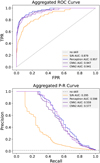 |
Fig. 12 Aggregated ROC and PR curves for the directly imaged companions dataset. We used ROC and PR AUCs to quantify of the scoring quality of the ML methods relative to S/N. The ROC curves measure the trade-off between TPR and FPR; however, they tend to be over-optimistic in highly balanced frameworks, such as in imaging data. The P-R curves measure the trade-off between precision and recall. |
4.3 Supplementary results on a simulation of PZ Tel B
In this section, we present a final test conducted using a simulated version of the molecular maps from Fig. 1. Thus far, all tests were applied to provide a quantitative measure on the performance of MLCCS methods, with the use of evaluation metrics (e.g. ROC curves, P-R curves and Confusion Matrix). Such metrics require clear labelling of the signals occurring in spaxels, to be able to distinguish true classifications from false ones. This requirement enforces the planet injections to be bounded inside a delimited aperture in the test set. However, in real observational cases, the signal simply decays spatially from the object into the rest of the frame, until it is too weak to be detected. Therefore, the motivation for this test was to find out if our MLCCS methods, while trained with spatially bounded signal injections, could still perform reliably on a realistic test case where the signal freely decays into the image. However, the lack of signal and noise labelling prevents the use of evaluation metrics to precisely quantify detections. Instead, those conclusive results are presented qualitatively, and require interpretation in conjunction with the quantitative outcomes from prior tests.
We performed such tests with synthetic variants of PZ Tel B spectra inserted at rest frame. We used three cubes of PZ Tel B in bad seeing conditions (from the third set of cubes in Table 1) in which we inserted planets with different signal strengths. The atmospheric characteristics of the inserted planets were assumed to be Teff = 2800 K, log g = 4.1 dex, and the composition included H2O, CO in a hydrogen and helium dominated atmosphere (cf. Sect. 3.2). As for the planet insertions, the centroid and Gaussian decay of the stellar PSF was calculated from the original data cubes in good and bad seeing conditions. The S/N were calculated within a 3.5 pixel aperture. Then, in opposition to the training set, the realistic insertion of the simulations were made using a free signal decay with no aperture bound. The left panel of Fig. 13 represents a benchmark insertion as a bright companion with an average H2O signal of S/N = 7.3, matching the signal strength of the original data under good seeing conditions. Additionally, we inserted dimmer planets in the noise at a lower signal strength corresponding to bad seeing conditions (S/N = 1 .22 for H2O). This realistic scenario does not enable the use of PR curves or a confusion matrix due to the absence of aperture delimitation between signal and noise. Therefore, results are presented qualitatively, and require interpretation in conjunction with the quantitative outcomes from prior tests.
We performed the tests twice, once for the H2O molecule, and a second time with the CO molecule. For each test, the CNNs are run using five template channels of the same molecule (with Teff = {2700; 2800; 2900; 3000; 3100} K and log 𝑔 = {3.7;4.3;4.1;4.1;4.1} dex respectively). The S/N is evaluated on an exact H2O template match (Teff = 2800 K, log 𝑔 = 4.1 dex). We trained and validated on the imaged companions mock data, excluding the three cubes that we reserve for testing. For this setting, the full automated training process, including hyperparameter search, took about eight hours. We note, nevertheless, that the final model could simultaneously evaluate all three flattened IFUs within seconds, generating scored data that we split and reshape back into three cubes. Fig. 13 shows scoring maps for one cube at various noise levels and for both molecules, along with S/N and CNN results under simulated poor seeing conditions. Notably, for an average S/N of 1.22 for the H2O map and 1.05 on the CO map (measured within a 3.5 pixels aperture), CNNs show a drastic enhancement on conspicuity in scoring maps. Additional results, presented in Figs. D.1 and D.2, show successful detection of simulated PZ Tel B signals on bad seeing conditions, namely at scaled-down average H2O S/N levels of 1/3rd (top) and 1/6th compared to the original good seeing conditions. Those results show that MLCCS is very robust for planet detection in challenging noise and observing conditions, especially in non-Gaussian i.i.d. environments.
4.4 Explainability of the models by ensuring spatial independence and generalisability to other instruments
Through this work, we have put emphasis on providing a clear explainable and interpretable ML framework to ensure that the model learns the right features. Thus, by preserving spatial independence, we forced MLCCS to focus on the transformed spectral dimension. This strategy prevents the algorithms from learning structural artefacts from the spatial dimension, such as the PSF, spurious spatial dependencies, or local noise structures, which could be deleterious for the explainability and generalisability of some results. Thus, we trained all supervised classification algorithms only on the RV extent of individual cross-correlated spaxels. Consequently, observing a clear tight aggregation of pixels in a spectroscopic image, instead of scattered pixels, increases confidence for the candidate detection, since we know that each pixel’s score is independent from its neighbour; this is clearly exemplified in Fig. 13. We also made tests to verify what the models are learning. First, we show in Appendix B.3 that in the presence of Gaussian noise structures, the CNNs are not be able to extract more information than the cross-correlation peak itself, and yield very similar performances as the S/N, as stated by (e.g., Gabbard et al. 2018). Second, we ran tests on the CO molecule, which contains strong symmetries, to show that MLCCS methods do learn specifically the cross-correlation patterns such as harmonics and auto-correlation from molecular signals (cf. Appendix B.4). As Hoeijmakers et al. (2018) and Mâlin et al. (2023) indicate, these patterns might be the result of overtones, related to the evenly spaced molecular lines in the template and spectrum of the exo-planet. These overtones are not used by the S/N statistic and may even decrease its score strength, but they do provide valuable information to the ML approaches. Third, although generally robust to small changes in the extent of the cross-correlation series, we report a light trend favouring more information in the cross-correlated series, which can be leveraged by MLCCS (cf. Appendix B.5). Finally, as CNNs can be implemented to be invariant to shift and stretches (Chaman & Dokmanic 2021), we successfully validated preliminary tests on invariance to RV shifts of the planet in the cross-correlation series. Such tests have important implications for detection capabilities, which are further discussed in Appendix B.5.
In order to delve deeper into the explainability of the framework, we also trained and tested for a wider range of models, which included L1 regularisation and variable selection oriented methods (e.g. Lasso, Random Forests etc) to understand how information is used in the RV dimension. We noticed that the variable selection methods would optimise towards using only the information at the cross-correlation peak and its immediate neighbourhood, but performed barely better than the S/N metrics. This indicates that the strong correlation between RV features prevents these models from performing a coherent variable selection (Toloşi & Lengauer 2011). The methods that partially or fully include L2 regularisation such as ElasticNet and Ridge are able to handle the correlations between RV features in a more consistent way: by setting a lower regularisation level and a higher L2 to L1 regularisation, we improved the results on ROC and PR AUC metrics. This means that if regularisation needs to be increased, for instance to improve the generalisability of the methods for noise from various targets, the L2 type should be favoured.
With the spatially independent training scheme, the proof of concept is not only useful for isolated spectra or spectroscopic imaging modes; it also ensures the flexibility to train and test MLCCS with various spectroscopic modes (e.g. IFS and slit spectroscopy), as it does not depend on the structure nor the order of the given spaxels. For example, the tests on the extracted spectra of companions dataset are valid for imaging spaxels as well as for long slit and single slit spectroscopy. In addition, CCS has proven to also work on transmission spectra (de Kok et al. 2013). Thus, by replacing tests on medium-resolution planetary emission spectra to high-resolution transmission spectra, and by adapting the noise sources, our approach could undergo future investigations in this direction. Potential challenges related to stellar contamination and variability may need to be investigated and addressed in this case.
Nevertheless, learning spatial information and the PSF could be a favourable by-product, according to the purpose and provided it is done and tested carefully. In this regard, the companion paper (Nath-Ranga et al. 2024) applies a variant of the MLCCS approach specifically tailored for high contrast imaging spectroscopy. They demonstrate that they can achieve higher detection performance than non-ML methods by effectively leveraging features in space and time dimensions of a cross-correlated IFS. As a trade-off, lower emphasis was put on the RV series, which were included as a discrete set of filters gathered around the expected planet’s RV, with the use of a unique full atmospheric template instead of a set of molecular template channels. Thus, the parallel and differentiated frameworks (i.e. learning molecular features vs. learning spatial features) emphasised different aspects that could be learned by CNNs. Together, both approaches consolidate each other in showing that ML can improve detection sensitivity to planetary signals in cross-correlated spectroscopic data. Future users should choose the framework according to the data and to the information they want to privilege and extract from it, or could use both to corroborate results.
 |
Fig. 13 Simulated molecular maps and reconstruction of the predicted classification scores by the S/N and CNN. Left: insertion of a simulated PZ Tel В signal in the real PZ Tel В noise cubes, with same location, Gaussian decay and average S/N = 7.3 as the real data shown as a molecular map in good seeing conditions. Middle-left: insertion of a signal in the PZ Tel B data with location and Gaussian decay of the original signal, but with an average S /N = 1.22 to emulate a signal in bad seeing conditions. Middle-right: S/N probability scores for bad seeing conditions. The planet is not detectable at S/N = 5. Right: CNN probability scores for bad seeing conditions. A very clear conspicuity improvement is observed in probabilistic map, clearly enhancing the planet’s visibility. |
5 Conclusion
Through this paper, we have introduced a novel approach, MLCCS, to merge ML and cross-correlation spectroscopy for exoplanet detection by leveraging molecular signatures in spectral data. As MLCCS techniques adopt a holistic approach in the cross-correlated spectral dimension, they are able to identify patterns from molecular signals, including harmonics and overtones. We show overall, that CNNs can operate effectively in non-Gaussian and non-i.i.d. environments to reveal sub-stellar companions embedded in complex noise structures. Thus, this approach addresses particular scenarios in which molecular mapping and CCS alone would fail to offer clear detections in the spectral dimension, while our companion paper by Nath-Ranga et al. (2024) addresses detections with emphasis in the spatial and temporal dimensions. Both papers strongly complement each other in tackling detection problems by leveraging dimensionalities differently in cross-correlated cubes, with the common purpose being the detection of planets embedded in spectroscopic noise.
Hence, through this work, we conducted two broad sets of experiments with dedicated test datasets in order to compare the performance of the MLCCS methods with a classical S/N statistic. In the first experiment, we assessed the performance of exoplanet detections under varying atmospheric characteristics in an unstructured stack of individual spectra. We found that MLCCS methods were able to discover 77 times more planets than the S/N for a false discovery rate constrained with an upper bound at 5%. This achievement is attributed to the CNNs’ use of multiple template filters, which enables an agnostic approach to exoplanet detection when atmospheric characteristics are unknown. Through additional tests, we also validated the capacity to combine different molecular templates to target a broader set of compositions. We also validated the invariance of our neural networks to RV shifts. Those two results have major implications for improving the flexibility in detecting unexpected planets in the data. In the second experiment, we showed that MLCCS enhanced the detection of companions in structured data such as imaging spectroscopy. Indeed, we could strongly improve the conspicuity on scoring maps despite the spatially independent training scheme.
By ignoring the spatial dimension, we focused on training MLCCS along the transformed spectral dimension. The goal was to ensure flexibility towards various spectroscopic instruments and observing modes for which cross-correlation methods have already been proven useful (e.g. with IFS data from VLT/SINFONI and JWST/MIRI Hoeijmakers et al. 2018; Patapis et al. 2022, and slit spectroscopy with CRIRES, Keck/OSIRIS and CRIRES+ de Kok et al. 2014; Petit dit de la Roche et al. 2018; Boldt-Christmas et al. 2024, for both emission and transmission spectra). Indeed, the method could in principle be adapted and tested for transmission spectra after appropriate adjustments to the data and templates. On a wider scope, this technique would be crucial for spectroscopic observations, which require relatively long observing times, as the signal strength may depend positively on integration time (e.g., Kiefer et al. 2021, for IFS) or even exposure and/or time resolution (i.e. Boldt-Christmas et al. 2024, on transmission spectra with CRIRES+). Our MLCCS methods are able to detect planets even under challenging noise conditions. This ability could offer a significant reduction in telescope time. Moreover, we emphasise that all of our tests were performed on individual or sub-combined exposure cubes; therefore, we strongly encourage further investigation in this direction. For a better generalisability, we would also aim for full invariance towards noise cubes of different targets observed with the same instrument to allow for even more robustness towards various seeing conditions.
Overall, our MLCCS methods showed capacity to improve the sensitivity to detect exoplanets and their molecules while offering robustness to systematic noise and sensitivity to molecular harmonics. This enhancement is crucial for exoplanet surveys in spectroscopic data (e.g., Agrawal et al. 2023), especially if they allow one to reduce the required telescope time. We expect this new approach to be beneficial to performing detection in cases where angular differential imaging (Marois et al. 2006) cannot be employed, when strong systematic noise subsists after data reduction (e.g., Hoeijmakers et al. 2018), and in poor observing conditions. Fortunately, existing archival data from VLT/SINFONI, CRIRES and new data inflow from VLT/ERIS, CRIRES+, JWST/NIRSpec will provide the chance to widely test, validate, and calibrate MLCCS towards extensions and applications with various spectroscopic modes. Specifically, future work should investigate the benefits of using MLCCS methods with the newest and future instruments for which cross-correlation based methods have proven their potential, such as the detectability of trace species in cool companions with JWST/MIRI (Patapis et al. 2022; Mâlin et al. 2023); the search for isotopologues in data from various instruments (Mollière & Snellen 2019; Zhang et al. 2021; Gandhi et al. 2023); or performance assessments of molecular mapping methods in challenging observation conditions with ELT/HARMONI (Houllé et al. 2021; Bidot et al. 2024; Vaughan et al. 2024).
Data availability
The codes are made publicly available on github in the form of a python library named MLCCS: https://github.com/eogarvin/MLCCS.
Acknowledgements
E.O.G., J.H., and S.P.Q. gratefully acknowledge the financial support from the Swiss National Science Foundation (SNSF) under project grant number 200020_200399. G.C. thanks the Swiss National Science 902 Foundation for financial support under grant number P500PT_206785. R.N.-R. and O.A. are funded by the Fund for Scientific Research (F.R.S.-FNRS) of Belgium, and acknowledge funding from the European Research Council (ERC) under the European Union’s Horizon 2020 research and innovation programme (grant agreement No 819155). The contributions of D.P. have been carried out within the framework of the NCCR PlanetS supported by the Swiss National Science Foundation under grants 51NF40_182901 and 51NF40_205606. D.P. acknowledges support of the Swiss National Science Foundation under grant number PCEFP2_194576. We thank Rico Landman as well as Chloe Fisher for their helpful comments. We also thank Felix Dannert and Philipp Huber for many insightful discussions and their valuable feedback regarding the figures. We thank the editor Dr. David Mouillet for the useful suggestions that improved our manuscript. We thank the referee Dr. Simon Petrus for the very careful review and propositions that allowed us to greatly improve the quality of the manuscript. We also thank the language editor Michael Coronado for his work which helped improve the manuscript. Author contributions: E.O.G. carried out all analyses, defined the optimisers and evaluation metrics and wrote the manuscript and codes. M.J.B. proposed the initial idea to use CNNs to detect exoplanets, and made propositions along the work to improve the structure of the manuscript. J.H. carried out the simulations of the planets and brown dwarfs and contributed to writing the related manuscript section. G.C. provided and reduced the real data cubes. J.S. tested the codes and the RV invariance under supervision of E.O.G. S.P.Q and N.F.M. provided guidance and administrative supervision along the project. All co-authors discussed the results and carefully commented on the manuscript. Python libraries: Our codes make extensive use of Keras (Chollet 2015), Matplotlib (Hunter 2007), Numpy (Harris et al. 2020), Pandas (McKinney et al. 2010), Photutils (Bradley et al. 2023), PyAstronomy (Czesla et al. 2019) and Scikit-learn (Pedregosa et al. 2011). The data preparation required the use of petitRADTRANS (Mollière et al. 2019).
Appendix A Molecular mapping: detections of CO and H2O in PZ Tel B
In this section, we report tentative “5σ” detections of H2O (cf. Fig. 1) and CO (cf. Fig. A.1) for PZ Tel B data obtained with molecular mapping. The presence of H2O and CO have been predicted by (Stolker et al. 2020) according to calculated abundance profiles in relation to the measured temperature on the object. For both Fig. 1 and A.1, the left IFU was observed on 04.05.2015 (Program ID: 093.C-0829 B), in four DITs of 60s with airmass 1.11, an average coherence time of 0.001931, and a start to end seeing from 0.77 to 0.72, which we define as the better observation conditions. The right IFU was observed on 28.07.2015 (Program ID: 093.C-0829 B) in 20 DITs of 10s with airmass 1.12, an average coherence time of 0.001931, and a start to end seeing from 1.73 to 1.54, which represent overall worse observation conditions relative to the right plot. The seeing seems to be a dominant factor in reducing the observation quality, but we also note that the exposure time is lower.
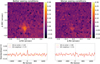 |
Fig. A.1 Molecular mapping detection of CO for real PZ Tel B data using cross-correlation for spectroscopy. This figure is an analogue to Fig. 1, applied to the CO molecule instead of H2O. It is even more obvious in the case of CO, that the cross-correlation and molecular maps fail to yield a clear peak under worse conditions. |
Appendix B Extended tests on the extracted spectra of companions
B.1 Interpretability of the results: the scaling factor α
To test the sensitivity of the results to varying levels of noise, we implemented the methods over different scale factors on the extracted spectra of companions dataset. The companions were inserted with different scale factors on the noise, as shown in Eq. (3). We tested for the values of α = {2; 5; 8; 11; 16; 21; 29; 41; 67}, which were respectively selected according to the following ROC AUC values of S/N: [0.55; 0.6; 0.65; 0.7; 0.75; 0.8; 0.85; 0.9; 0.95]. We depict the most illustrative cases in Fig. B.1 to show the variations of the relative gains across methods, and that they depend on different levels of noise.
Fig. B.1 shows that the relative gain of using MLCCS methods do indeed depend on the noise level. For an excessively small or big scale factor, the improvement differential between the S/N and the MLCCS methods will be almost null. If signals are drowned into the noise, all classifiers will lose their skills (cf. α = 2 in Fig. B.1). If signals are extremely strong, the noise has no influence and any statistic or algorithm tends towards a perfect classifier (cf. α = 67 in Fig. B.1). However, there is a range of noise levels, between the extremes, for which it is worth using MLCCS due to the gain in detection performance.
 |
Fig. B.1 ROC AUC improvements and relative gains of MLCCS for a range of α values. The scale factors of α = [2,5,11, 21, 67] (from left to right), were selected to illustrate that MLCCS offers a smaller improvement relative to S/N for very small α (extreme noise) and very large α (extreme signal). The scaling factor a is inversely proportional to the strength of the noise. |
B.2 Flexibility towards compositions of the planets: leveraging template multiplicity
 |
Fig. B.2 Scoring and classification of the S/N and CNN for planets cross-correlated with template channels of CO and H2O. Overall, 12161 planets containing either CO, H2O, or both, alongside with other molecules, were inserted with a scaling factor of 8. Left: Aggregated ROC curves as already shown in Fig. 11 from Sect. 4.1. Middle and Right: Amount of planets that can be recovered by the perceptron and the CNN, for different characteristics (i.e. all planets, those containing either CO or H2O, or both. |
In this section, we investigate how varying the composition of the template channels enables one to search for a wider range of companions with CNNs while increasing flexibility, agnosticity, and detection sensitivity to planets. Thus, for this example, we used a total of ten channels. We included five template channels of CO in parallel to five templates of H2O for each CNN. Thus, for both molecules this yielded Teff = [1200,1400,1600,2000,2500], while the CO templates had log(g) = [2.9,4.1,4.5,4.1,5.3] and the H2O templates differ with log(g) = [4.1,3.5,4.1,4.1,5.3]. As usual, the templates were chosen to cover the parameter space evenly (cf. Sect. 3.2), while alternating the composition. No template contained both molecules together; we only used singletons. The first template (i.e. H2O with Teff = 1200 and log(g) = 4.1) served as “base template” for the S/N and perceptron that can only be fed with one channel and can detect only one molecule at a time.
We ran tests on the extracted spectra of companions mock data. The test case used a similar setting as in the main framework (as described in Sect. 3.3) except for the fact that 50% of the injected planets contained H2O, CO, or a mixture of both (amongst other molecules). The rest contained either pure noise or planets with other molecular mixtures, excluding H2O and CO. For comparability with the main test setting, all planets were also injected with a scale factor α = 8. The labels were provided to the algorithms to indicate that a detection should contain at least one of the two molecules.
The ROC curves are shown in Fig. B.2. First, the ROC AUC of the S/N is low, with a value of 0.591, although we kept the same base H2O template as for the main test in Fig. 11. This is not surprising, since the S/N can only work with one template at a time and can only detect planets with water. On the other hand, the ROC AUCs show how the CNNs gain performance when allowed to search not only across atmospheric parameters, but also across molecular compositions. Such results are very promising for the implementation of agnostic frameworks in spectroscopic datasets. We also note that, at equal α value, the perceptron seems to have gained performance. It increases from a ROC AUC of 0.792 in Fig 11 to 0.815 in Fig. B.2. For this reason, we also investigated what types of planets the methods are able to find.
The middle plot in Fig. B.2 shows the percentage of total planets of interest that the perceptron is able to find. The perceptron finds 41% of the planets in total. First, we observe that, although the perceptron was fed with the base molecular template of H2O, it learns to detect CO more easily than H2O. We emphasise that in the main test (i.e. where we search only for planets with H2O), the perceptron does not detect any planets that do contain CO without H2O. Thus, those results are not accidental and are intrinsic to the fact that the perceptron learned some systematic and deterministic patterns of CO, even when the planet is cross-correlated with a different molecule. Then, we observe that by using multiple template channels with composition variations, that CNN1 is able to find up to 74% of the total planets. It most consistently finds companions that contain both molecules. This result is very interesting, since all template channels consist of only one molecule at a time; this means the CNNs can combine the information provided separately to strengthen the detection of objects that satisfy more criteria. In addition, it also detects planets that contain either of each molecule, showing high flexibility for composition.
B.3 Explainability of the framework: idealistic Gaussian noise
 |
Fig. B.3 Tests conducted on planetary signals (H2O) embedded in idealistic simulated Gaussian noise. Left: ROC curves and AUC showing that neural networks are barely able to perform better than the S/N. Middle-Left and Middle-Right: Frequency distributions of aggregated scores assigned to the negative group (red) against the positive group (blue) for the S/N (left) and the CNN (right) in the presence of Gaussian noise. The CNNs are not able to separate the scores and improve conspicuity as well as in the case of non-Gaussian noise. Right: Classification predictions under a Gaussian noise regime, given a FDR≤ 5%. The use of MLCCS to extract signals becomes ineffective under Gaussian noise, as they are not able to extract more information than the S/N. |
In this section, we tested and briefly discuss the results of the MLCCS methods for signal detection in an idealistic framework of identically and independently distributed Gaussian noise environment, as opposed to the main tests on real data from SINFONI. In order to do so, we built Gaussian replicates of the SINFONI noise. This means that for every SINFONI noise spectrum (cf. Sect. 3.1, we estimated the mean and variance. Then, we simulated a Gaussian analogue of the noise series using the estimated mean and variance parameters. After this, all procedures we used to insert the planets in the noise were the same as in Sect. 3.3. As we can observe from the left panel in Fig. B.3, in the context of Gaussian i.i.d. noise environments, the MLCCS methods perform exactly as the S/N in terms of ROC AUC. This means that the algorithms are only able to learn as much information as the S/N provides. We can also observe this in the middle-right panel from Fig. B.3. Indeed, the CNNs were not able to transform the data to separate the scores as efficiently as in the tests on non-Gaussian data (cf. middle panel in Fig. 10).
In fact, such results were expected, since the cross-correlation provides the maximum likelihood solution for an optimal template in the case where the noise is Gaussian (Brogi & Line 2019). This also means that the cross-correlation (as a generalisation of the Pearson’s correlation) only provides a complete description of the similarity between a spectrum and a template when the random noise is Gaussian. Therefore, under pure Gaussian i.i.d. noise, methods such as matched filtering or S/N methods on cross-correlation would perform optimally in extracting signals. In such cases, CNNs would not be expected to perform better than the baseline, since there is no additional information to extract (Gabbard et al. 2018). This is what we can observe with the results of our tests on Gaussian i.i.d. noise. We attribute the very small performance improvement of the CNNs here to remaining and persistent molecular harmonics that can overcome the Gaussian noise. Nevertheless, it is clear that if the signal is embedded in pure Gaussian noise, the MLCCS methods do not offer great improvements. This also acts as a proof of the non-Gaussianity of the realistic noise; the cross-correlation carries over the non-Gaussian i.i.d. noise pattern structures, which enable MLCCS to learn information from. We also note in the fourth panel of Fig. B.3, that the S/N is detecting fewer planets than the non-Gaussian framework. This also shows that S/N detection significance and uncertainties are mis-estimated when we assume Gaussian noise on non-Gaussian data, because the detection capabilities change according to the nature of the noise.
B.4 Explainability of the results: molecular harmonics
To improve the explainability of the framework, we investigated what the CNNs and the perceptron are able to learn. Such explainable frameworks in ML are fundamental to orient future research towards real data applications. As we suspected that MLCCS should be able to learn symmetries in the cross-correlated series as well as molecular harmonics, we extended the tests to the CO molecule only, which is known to host strong harmonics in its cross-correlated sets (Fig. B.5). We built a new dataset in the same way as in Sect. 3.3. This time, it is constituted of 50% of planets with CO. We observe in Fig. B.4, that for a similar S/N performance in terms of ROC AUC, it is easier to detect CO. Indeed, the perceptron achieves an AUC of 0.902 and the CNNs reach an AUC of 0.913. Such results proving the efficacy in detecting CO are corroborated by the molecular maps in Appendix D.
The reason for this is that CO has clear and very strong harmonics, as shown in Fig. B.5. Those are easily learned using holistic approaches such as MLCCS on the whole cross-correlated series. Such harmonics are still visible and can be detected up to RVs of ±750, even in the case where the templates are not matching exactly with the planet’s characteristics (cf. example with the right panel of Fig. B.5). This relates to the fact that the ML algorithms are leveraging correlated patterns in the features of the cross-correlated series, as previously discussed in Sect. 4.4. On the other hand, we observe that water has a clear cross-correlation peak that dies off at about RV = ±200. Its symmetric patterns are rather discrete but visible on the left panel. Thus, we see a clear difference in the strength of the auto-correlation patterns caused by harmonics and symmetries in the cross-correlated series for CO compared to H2O molecules, explaining the performance improvement with CO templates.
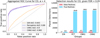 |
Fig. B.4 Scoring and classification of the S/N and CNN for cross-correlated spectra with the CO molecule. Left: Quantification of scoring performance with receiver operating characteristic curves (ROC). The plot shows the improvements in the ROC trade-off between TPR and FPR. The improvement is measured in terms of area under the ROC curves (AUC). The CNNs provide even better performance in finding CO molecules while limiting increments in FPR, as compared to the main tests. Right: Maximal amount of planets with CO that can be recovered in the mock data by the S/N, perceptron (PCT) and both CNNs, within a FDR ≤ 5% bound. |
 |
Fig. B.5 Cross-correlated templates showing molecular harmonics and symmetric patterns for H2O and CO. Left: Cross-correlation of templates with themselves (with Teff = 1200 and log(g) = 4.1),allowing to verify how the molecular harmonics behave for H2O and CO. The cross-correlation shows clear symmetric patterns for both molecules and strong harmonic patterns for CO. Right: Cross-correlation of different templates with each other, i.e. one template of template of Teff = 1200 and log(g) = 4.1 and one template of Teff = 2200 and log(g) = 4.1 as shown in the right panel. |
B.5 Robustness and invariance: the cross-correlation series and radial velocity shifts
We ran tests to evaluate the robustness and invariance properties of our CNNs regarding variations in the cross-correlation series and shifts in RV. We first tested the effect of widening and shortening the extent of the cross-correlated series and widening the RV step. The methods’ applicability is generally robust to such variations, as they involve only minor changes in the ROC AUC that consistently remains above 0.8 for the CNNs. Nevertheless, we generally observed that having more RV features offered better performance. For instance, lengthening the series up to ±3000km s slightly increased the ROC AUC (between 0.11 to 0.13 points for all ML methods compared to the main test). However, this came with a cost in increased computational time. For tests where we shortened the series (e.g. ± 1200km s−1) or enlarged the RV steps (e.g. RV steps of five or ten), we observed an accelerated convergence of the optimisation process, but a slight decrease of the performance, although the AUC of the CNNs stay above 0.8. Finally, we tested more drastic changes, with a cross-correlation of ±500km s−1 and RV steps of 10, overall reducing the RV features to only 100 points. In this case, the performance drops, with ROC AUCs reaching 0.724 and 0.728 for CNN1 and CNN2, against 0.685 for the perceptron and 0.652 for the S/N. Despite the relative robustness of the CNNs to changes in the amount of RV features, it needs a reasonable amount of information to be able to learn structures in the cross-correlation.
The second test was performed to evaluate invariance properties towards shifts in RVs. RV invariance is useful in the perspective that planets in real data have varying radial velocities that create shifts and stretches in fine pattern structures of the cross-correlated spectrum. So far, for comparability of the results with the S/N metric (which requires prior knowledge or visual inspection of the peak’s RV), all tests were performed on planets present at rest frame. However, CNNs that were trained on a fixed RV could not generalise to varying RV shifts. Thus, we implemented variations of our dataset that include RV shifts occurring uniformly randomly around the rest frame. We tested realistic RV shifts with bounds at ± 100km s−1, as well as a more conservative scenario to challenge the CNNs with large RV shifts up to ±500km s−1. The conservative results from the second test are shown in Fig. B.6. Our results on both scenarios converged towards the conclusion that our CNNs are robust in detecting planets and their molecules in cross-correlations from Doppler-shifted spectra in the test set. Finally, true invariance (Mouton et al. 2020) to RV shifts is only proven when the test set is evaluated on a shift that was previously unseen in the training and validation sets. Thus, such tests were also evaluated. The most conservative scenario included training of MLCCS on RVs of [−225.0; −276.8; 236.5; 176.7; 392.2; −413.1] km s−1, validated on an RV shift of 139.4 km s−1 and tested on an RV of −475.0 km s−1, and it returned an ROC AUC of 0.805 for CNN1 against 0.68 for the perceptron. The lower performance of CNN2 is due to its more complex architecture and regularisation schemes mentioned in Sect 2.3. Thus, CNN1 displays a high degree of invariance even in a conservative scenario. The preliminary proofs on RV shifts have important implications for the generalisation of the methods to real data, as shift invariant CNNs would be necessary to detect planets for which we do not have prior orbital constraints. On the other hand, training on fixed RVs can be preferred when prior orbital information is available and we focus the use of MLCCS for detection of molecular species.
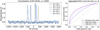 |
Fig. B.6 Invariance tests on RV shifts. Left: Example of shifts in RV implemented between ±500km s−1. The H2O signals were voluntarily pushed up to a scaling factor of α = 5000 only for visualisation purposes. Right: Associated ROC AUC performance on RV shifted signals inserted with a scale factor of α = 8 yielding faint signals, as in the baseline framework. |
Appendix C Extended test results on the direct imaging of companions dataset
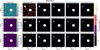 |
Fig. C.1 Reconstruction of classification scores by S/N, PCT, and CNN2 for various test cases (results of CNN1 are redundant). Equivalent benchmarking is challenging, but objectively applied thresholds highlight the distinct behaviour of each method’s scores. First column: Scores are displayed for the three methods in all test cases. From second to sixth column: Classification maps shown according to increasing thresholds, set to T = {1; 2; 3; 4; 5} for S/N and to T = {0.1; 0.3; 0.5; 0.7; 0.9} for MLCCS. Four colours represent the confusion matrix elements: true positives (TP), false positives (FP), false negatives (FN), and true negatives (TN). |
In this section, we show the results of the three test cases of the imaged brown dwarf datasets. These test datasets were constructed in the same way as their training and validation sets, namely by inserting aperture delimited planets. The synthetic planets were inserted with a random Gaussian ellipse size, shape and location, hence the aperture size and centre is adaptive to the insertion properties. The aperture delimitation allowed to use the confusion matrix to evaluate the results, after the predictive classification was performed for a given threshold.
The results are visible in the three test cases in Fig. C.1, as scoring maps on the very left, and classification results according to increasing thresholds in the five columns on the right. Due to space constraints and to avoid redundancy, we only show the outcomes of CNN2; CNN1 results were very similar and equivalent. Overall, the plots show that the MLCCS classifiers generally enhance the prediction certainty. In terms of scoring results, there is a clear conspicuity improvement offered by the MLCCS methods. While the planet is barely visible in the S/N and really blends into the noise, it clearly appears in the probability scores of MLCCS methods. In fact, they are visible even if the detection score is low, because the noise is very clearly classified with high “negative” confidence (i.e. low probability to belong to the positive group). Figure C.2 aims to quantify the quality of the scores using P-R curves, described in Sect. 4. In case 1, the perceptron outperforms the CNNs, with an AUC of 0.526 against 0.459. In case 2, only CNN2 outperforms the perceptron, showing an AUC of 0.628 against 0.621; CNN1, however, shows a weaker AUC. In case 3, both CNNs outperform the perceptron, with AUCs of 0.672 and 0.665 for CNNs against 0.659 for S/N. Overall, all ML methods perform relatively equivalently, but show significant improvement compared to the S/N baseline that has an AUC between 0.288 and 0.308 over the plots.
The enhanced prediction certainty is also visible with the classifications at low thresholds (cf. columns 2 to 5 in Fig. C.1). This fact stands out particularly at the two first thresholds. For example, T = 0.1 on MLCCS probability scores shows significantly fewer FPs than T = 1 and T = 2 of the S/N for all cases. While increasing the thresholds neural networks are better able to reduce false positives while better preserving true positives. By comparing a threshold at T = 0.3 for MLCCS methods against T = 3 for the S/N metric, we can observe more TPs for fewer FPs; specifically, test case 1 presents eight TPs for five FPS for S/N. Test cases 2 and 3 present about double amount of TPs for CNNs against S/N for similar to half the amount of FPs.
To control that the low variability in the probability scores attributed to noise were not a result of overfitting, we conducted two categories of tests. Obviously, all tests cases were run on GQ lup B noise cubes, and trained on 17 out of 19 cubes as we exclude the validation and test sets, meaning that no noise spaxel is seen twice at any time. Yet, test cases 2 and 3 were output by an ML model that was validated on another GQ lup B noise cube, which implies that it was optimised according to the correct target noise. For test case 1, we used a target noise cube of PZ Tel B to validate the model during training and investigate if the results remain stable (i.e. if the model does not overfit). This means that the model was optimised regarding a different noise distribution, and can still detect the simulated brown dwarf in a GQ lup B noise test cube. The probability scores attributed to the noise look less smooth, but the conspicuity is still very clear. This test is a first step towards investigating noise invariance across targets, for a given instrument. Nevertheless, it is crucial to emphasise that despite our precautions, the risk for moderate overfitting remains, even when the training set was not exposed to the spaxels of the validation or test set, due to the fact that other exposure cubes from the same target still remain in the training set. However, we highlight that the scenario of training and testing on similar noise cubes is not unlikely. In a real case, it would be possible to train the models using noise from parts of exposure cubes that we expect to be empty, and test for regions of the leftover cubes where the planet is likely to be present. Yet, this procedure involves prior information about the orbit, inclination and expected location of the planet, from RV or astrometric data. If we rather focus on a blind search to discover new planets without prior information, we must indeed test the capacity of the networks to become invariant to noise across targets, which should be a focus for future work.
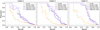 |
Fig. C.2 Precision-recall curves related to the three test cases. Each curve is computed based on the scores attributed to each spaxel retrieved from an image cube. The curves represent the trade-off between precision and recall achieved by the scores. A classifier with no skill (grey dashed line) is proportional to the number of positive values in the data; it would perform random, uninformed classification of 0.1% of the of the data to the positive class. |
Appendix D Extended results on the PZ Tel B simulations
This section shows the full tests on the realistic PZ Tel B simulations inserted in its real SINFONI K-band noise at medium resolution. Details on the characteristics of the simulated planet are already described in Sect. 4.3. Figure D.1 shows the results for two different noise levels (i.e. α scaling factor values) for (1) and (2). The first column of all plots shows a simulated reproduction of PZ Tel B under good conditions. For the three original real data cubes in good conditions, we measured the average S/N as β = {7.89; 5.893; 7.303} in an aperture of 3.5 pixels, and calculated a decay rate of a Gaussian PSF as δ = {3.595; 3.955; 3.701}. Then, we inserted the simulated brown dwarf companions in respective noise cubes from bad observing conditions, with the corresponding S/N and Gaussian decay rate using a re-scaling factor of respectively α = {121.23; 116.75; 113.85}.
The second columns of all plots show simulated insertions in bad conditions. For plot (1), the scaling factor α is cut down by 3 to align the parameters of β and γ with measurements on real data in bad conditions. This results in average S/N of β = {2.666; 2.07; 2.538}. For plot (2), we challenged the MLCCS models to a more extreme case; the simulated PZ Tel B was inserted at a scale factor α cut down by a factor of 6, yielding an extremely faint average S/N of β = {1.105; 0.997; 1.223}, hardly visible using the detection statistic. We applied CNN2 to obtain probability score maps on all cases (right column). Even when the S/N fails to find the brown dwarf in its scoring map, the CNN is able to reveal it. Analogue tests are run and confirmed for CO in Fig. D.2.
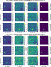 |
Fig. D.1 Scoring results of H2O for PZ Tel B simulations in its real noise. Subfigures 1 and 2, column 1: Synthetic brown dwarf insertion with its original average signal strength and decay representing good seeing conditions. Subfigure 1 and 2, col. 2: Insertion of the brown dwarf at 1/3 (Subfigure 1) and at 1/6 (Subfigure 2) of the original signal strength, using noise from the bad seeing conditions. Subfigure 1, 2; col. 3,4: S/N maps (col. 3) and CNN maps (col. 4) showing the scoring results for the insertions in bad seeing conditions from col. 2. |
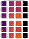 |
Fig. D.2 Scoring results of CO for PZ Tel B simulations in its real noise. Subfigures 3 and 4, column 1: Synthetic brown dwarf insertion with its original average signal strength and decay representing good seeing conditions. Subfigure 3 and 4, col. 2: Insertion of the brown dwarf at 1/3 (Subfigure 1) and at 1/6 (Subfigure 2) of the original signal strength, using noise from the bad seeing conditions. Subfigure 3,4; col. 3,4: S/N maps (col. 3) and CNN maps (col. 4) showing the scoring results for the insertions in bad seeing conditions from col. 2. |
References
- Abuter, R., Schreiber, J., Eisenhauer, F., et al. 2006, New Astron. Rev., 50, 398 [Google Scholar]
- Agrawal, S., Ruffio, J.-B., Konopacky, Q. M., et al. 2023, AJ, 166, 15 [NASA ADS] [CrossRef] [Google Scholar]
- Amara, A., & Quanz, S. P. 2012, MNRAS, 427, 948 [Google Scholar]
- Benjamini, Y., & Hochberg, Y. 1995, J. R. Statis. Soc. Ser. B, 57, 289 [CrossRef] [Google Scholar]
- Bidot, A., Mouillet, D., & Carlotti, A. 2024, A&A, 682, A10 [NASA ADS] [CrossRef] [EDP Sciences] [Google Scholar]
- Boldt-Christmas, L., Lesjak, F., Wehrhahn, A., et al. 2024, A&A, 683, A244 [NASA ADS] [CrossRef] [EDP Sciences] [Google Scholar]
- Bonse, M. J., Garvin, E. O., Gebhard, T. D., et al. 2023, AJ, 166, 71 [NASA ADS] [CrossRef] [Google Scholar]
- Bradley, L., Sipőcz, B., Robitaille, T., et al. 2023, https://doi.org/18.5281/zenodo.7946442 [Google Scholar]
- Briechle, K., & Hanebeck, U. D. 2001, SPIE, 4387, 95 [NASA ADS] [Google Scholar]
- Brogi, M., & Line, M. R. 2019, AJ, 157, 114 [Google Scholar]
- Brogi, M., De Kok, R., Birkby, J., Schwarz, H., & Snellen, I. 2014, A&A, 565, A124 [NASA ADS] [CrossRef] [EDP Sciences] [Google Scholar]
- Cantalloube, F., Gomez-Gonzalez, C., Absil, O., et al. 2020, SPIE, 11448, 1027 [Google Scholar]
- Chaman, A., & Dokmanic, I. 2021, in Proceedings of the IEEE/CVF Conference on Computer Vision and Pattern Recognition, 3773 [Google Scholar]
- Charnay, B., Bézard, B., Baudino, J.-L., et al. 2018, ApJ, 854, 172 [Google Scholar]
- Chollet, F. 2015, keras, https://github.com/fchollet/keras [Google Scholar]
- Cugno, G., Patapis, P., Stolker, T., et al. 2021, A&A, 653, A12 [NASA ADS] [CrossRef] [EDP Sciences] [Google Scholar]
- Czesla, S., Schröter, S., Schneider, C. P., et al. 2019, Astrophysics Source Code Library [record ascl:1906.010] [Google Scholar]
- Davis, J., & Goadrich, M. 2006, in Proceedings of the 23rd international conference on Machine learning, 233 [CrossRef] [Google Scholar]
- de Kok, R. J., Brogi, M., Snellen, I. A., et al. 2013, A&A, 554, A82 [NASA ADS] [CrossRef] [EDP Sciences] [Google Scholar]
- de Kok, R. J., Birkby, J., Brogi, M., et al. 2014, A&A, 561, A150 [NASA ADS] [CrossRef] [EDP Sciences] [Google Scholar]
- Fawcett, T. 2006, Pattern Recog. Lett., 27, 861 [CrossRef] [Google Scholar]
- Fisher, C., Hoeijmakers, H. J., Kitzmann, D., et al. 2020, AJ, 159, 192 [NASA ADS] [CrossRef] [Google Scholar]
- Gabbard, H., Williams, M., Hayes, F., & Messenger, C. 2018, Phys. Rev. Lett., 120, 141103 [NASA ADS] [CrossRef] [Google Scholar]
- Gandhi, S., de Regt, S., Snellen, I., et al. 2023, ApJ, 957, L36 [NASA ADS] [CrossRef] [Google Scholar]
- Gu, J., Wang, Z., Kuen, J., et al. 2018, Pattern Recog., 77, 354 [NASA ADS] [CrossRef] [Google Scholar]
- Guillot, T. 2010, A&A, 520, A27 [NASA ADS] [CrossRef] [EDP Sciences] [Google Scholar]
- Gulli, A., & Pal, S. 2017, Deep Learning with Keras (Birmingham, UK: Packt Publishing Ltd) [Google Scholar]
- Haffert, S., Bohn, A., De Boer, J., et al. 2019, Nat. Astron., 3, 749 [CrossRef] [Google Scholar]
- Harris, C. R., Millman, K. J., van der Walt, S. J., et al. 2020, Nature, 585, 357 [NASA ADS] [CrossRef] [Google Scholar]
- Hayoz, J., Cugno, G., Quanz, S. P., et al. 2023, A&A, 678, A178 [NASA ADS] [CrossRef] [EDP Sciences] [Google Scholar]
- Hoeijmakers, H., Schwarz, H., Snellen, I., et al. 2018, A&A, 617, A144 [NASA ADS] [CrossRef] [EDP Sciences] [Google Scholar]
- Houllé, M., Vigan, A., Carlotti, A., et al. 2021, A&A, 652, A67 [NASA ADS] [CrossRef] [EDP Sciences] [Google Scholar]
- Hunter, J. D. 2007, Comput. Sci. Eng., 9, 90 [NASA ADS] [CrossRef] [Google Scholar]
- Jenkins, J. S., Pavlenko, Y. V., Ivanyuk, O., et al. 2012, MNRAS, 420, 3587 [NASA ADS] [Google Scholar]
- Jensen-Clem, R., Mawet, D., Gonzalez, C. A. G., et al. 2017, AJ, 155, 19 [Google Scholar]
- Kiefer, S., Bohn, A. J., Quanz, S. P., Kenworthy, M., & Stolker, T. 2021, A&A, 652, A33 [NASA ADS] [CrossRef] [EDP Sciences] [Google Scholar]
- Konopacky, Q. M., Barman, T. S., Macintosh, B. A., & Marois, C. 2013, Science, 339, 1398 [Google Scholar]
- Krizhevsky, A., Sutskever, I., & Hinton, G. E. 2012, Advances in Neural Information Processing Systems (New York: Curran Associates, Inc.), 25 [Google Scholar]
- Line, M. R., Stevenson, K. B., Bean, J., et al. 2016, AJ, 152, 203 [NASA ADS] [CrossRef] [Google Scholar]
- Madhusudhan, N., Amin, M. A., & Kennedy, G. M. 2014, ApJ, 794, L12 [Google Scholar]
- Madhusudhan, N., Piette, A. A., & Constantinou, S. 2021, ApJ, 918, 1 [NASA ADS] [CrossRef] [Google Scholar]
- Malek, S., Melgani, F., & Bazi, Y. 2018, J. Chemom., 32, e2977 [CrossRef] [Google Scholar]
- Mâlin, M., Boccaletti, A., Charnay, B., Kiefer, F., & Bézard, B. 2023, A&A, 671, A109 [NASA ADS] [CrossRef] [EDP Sciences] [Google Scholar]
- Marois, C., Lafreniere, D., Doyon, R., Macintosh, B., & Nadeau, D. 2006, ApJ, 641, 556 [NASA ADS] [CrossRef] [Google Scholar]
- Márquez-Neila, P., Fisher, C., Sznitman, R., & Heng, K. 2018, Nat. Astron., 2, 719 [CrossRef] [Google Scholar]
- McKinney, W., et al. 2010, in Proceedings of the 9th Python in Science Conference, 445, Austin, TX, 51 [Google Scholar]
- Mollière, P., & Snellen, I. 2019, A&A, 622, A139 [NASA ADS] [CrossRef] [EDP Sciences] [Google Scholar]
- Mollière, P., van Boekel, R., Bouwman, J., et al. 2017, A&A, 600, A10 [Google Scholar]
- Mollière, P., Wardenier, J., van Boekel, R., et al. 2019, A&A, 627, A67 [NASA ADS] [CrossRef] [EDP Sciences] [Google Scholar]
- Mollière, P., Molyarova, T., Bitsch, B., et al. 2022, ApJ, 934, 74 [CrossRef] [Google Scholar]
- Morley, C. V., Marley, M. S., Fortney, J. J., et al. 2014, ApJ, 787, 78 [Google Scholar]
- Morley, C. V., Mukherjee, S., Marley, M. S., et al. 2024, ApJ, submitted [arXiv:2402.00758] [Google Scholar]
- Mouton, C., Myburgh, J. C., & Davel, M. H. 2020, Stride and Translation Invariance in CNNs (Berlin: Springer International Publishing), 267 [Google Scholar]
- Nath-Ranga, R., Absil, O., Christiaens, V., & Garvin, E. O. 2024, A&A, 689, A142 [NASA ADS] [CrossRef] [EDP Sciences] [Google Scholar]
- Nixon, M. C., & Madhusudhan, N. 2021, MNRAS, 505, 3414 [NASA ADS] [CrossRef] [Google Scholar]
- Nowak, M., Lacour, S., Mollière, P., et al. 2020, A&A, 633, A110 [NASA ADS] [CrossRef] [EDP Sciences] [Google Scholar]
- Öberg, K. I., Murray-Clay, R., & Bergin, E. A. 2011, ApJ, 743, L16 [Google Scholar]
- O’Shea, K., & Nash, R. 2015, arXiv e-prints [arXiv:1511.08458] [Google Scholar]
- Patapis, P., Nasedkin, E., Cugno, G., et al. 2022, A&A, 658, A72 [NASA ADS] [CrossRef] [EDP Sciences] [Google Scholar]
- Pedregosa, F., Varoquaux, G., Gramfort, A., et al. 2011, J. Mach. Learn. Res., 12, 2825 [Google Scholar]
- Petit dit de la Roche, D., Hoeijmakers, H., & Snellen, I. 2018, A&A, 616, A146 [CrossRef] [EDP Sciences] [Google Scholar]
- Petrus, S., Bonnefoy, M., Chauvin, G., et al. 2021, A&A, 648, A59 [EDP Sciences] [Google Scholar]
- Petrus, S., Whiteford, N., Patapis, P., et al. 2024, ApJ, 966, L11 [NASA ADS] [CrossRef] [Google Scholar]
- Pham, D., & Kaltenegger, L. 2022, MNRAS, 513, L72 [NASA ADS] [CrossRef] [Google Scholar]
- Ruffio, J.-B., Macintosh, B., Konopacky, Q. M., et al. 2019, AJ, 158, 200 [Google Scholar]
- Saito, T., & Rehmsmeier, M. 2015, PloS one, 10, e0118432 [NASA ADS] [CrossRef] [Google Scholar]
- Seifahrt, A., Neuhäuser, R., & Hauschildt, P. 2007, A&A, 463, 309 [NASA ADS] [CrossRef] [EDP Sciences] [Google Scholar]
- Snellen, I., De Kok, R., De Mooij, E., et al. 2010, Proc. Int. Astron. Union, 6, 208 [CrossRef] [Google Scholar]
- Stolker, T., Bonse, M. J., Quanz, S. P., et al. 2019, A&A, 621, A59 [NASA ADS] [CrossRef] [EDP Sciences] [Google Scholar]
- Stolker, T., Quanz, S. P., Todorov, K. O., et al. 2020, A&A, 635, A182 [EDP Sciences] [Google Scholar]
- Stolker, T., Haffert, S. Y., Kesseli, A. Y., et al. 2021, AJ, 162, 286 [NASA ADS] [CrossRef] [Google Scholar]
- Toloşi, L., & Lengauer, T. 2011, Bioinformatics, 27, 1986 [CrossRef] [Google Scholar]
- Vasist, M., Rozet, F., Absil, O., et al. 2023, A&A, 672, A147 [NASA ADS] [CrossRef] [EDP Sciences] [Google Scholar]
- Vaughan, S. R., Birkby, J. L., Thatte, N., et al. 2024, MNRAS, 528, 3509 [NASA ADS] [CrossRef] [Google Scholar]
- Waldmann, I. 2016, ApJ, 820, 107 [NASA ADS] [CrossRef] [Google Scholar]
- Xuan, J. W., Wang, J., Ruffio, J.-B., et al. 2022, ApJ, 937, 54 [NASA ADS] [CrossRef] [Google Scholar]
- Zhang, Y., Snellen, I. A., Bohn, A. J., et al. 2021, Nature, 595, 370 [NASA ADS] [CrossRef] [Google Scholar]
All Tables
All Figures
|
Fig. 1 Molecular maps of H2O for real PZ Tel B data using CCS. This figure shows a real case example where the noise structures may reduce detection capabilities of cross-correlation methods. The brown dwarf was observed under good conditions (airmass: 1.11, Seeing start to end: 0.77–0.72) and lower conditions (airmass: 1.12, Seeing: 1.73-1.54), cf. Appendix A for full details on observing conditions. Upper plots show molecular maps of PZ Tel B, while the lower plots show the cross-correlation series along the radial velocity (RV) support for pixels at the centre of the object, and within the object’s brightness area. While the brown dwarf should appear at the same spatial coordinates for respective RV locations in both cases (cf. vertical lines), it is clearly visible when conditions are good, but hardly visible on equal scales under lower conditions. |
| In the text | |
|
Fig. 2 Flowchart representing the methods, scoring, and classification workflows presented across sections. Each cross-correlated spatial pixel (spaxel) is treated as an independent instance and is passed through a classifier of static (statistic) or a dynamic (learning algorithm) type. The methods will evaluate the RV series and yield scoring metrics (e.g. a statistic or probability score). In order to perform classification, the scores need to first be separated using a meaningful threshold. The current standard classification scheme is yield by the S/N on the cross-correlation peak at the planet’s RV. We propose to analyse the RV series in a holistic approach using ML to detect the planets and their molecules, and use the resulting probability scores. |
| In the text | |
|
Fig. 3 Illustration of the shape and size of one cross-correlated dataframe. Each row is a sample and represents a cross-correlated spaxel (CC spaxel). The RV steps are called features, and the elements of the last column Y are the categorical labelling indicating the presence of a planet or molecule of interest in the spectra. One whole cross-correlated dataframe as above is named a template channel; it results from the cross-correlation of the whole spectral dataset (i.e. all samples) with a unique template. |
| In the text | |
|
Fig. 4 Architecture of the perceptron. This simple one-layer neural network analyses the values of a whole cross-correlation series in a holistic approach to detect the presence of a molecular signal. |
| In the text | |
|
Fig. 5 Example of the application of a CNN on one cross-correlated spectrum. For each sample of a cross-correlation N, and for all M template channels, the convolution filter runs across the channels and along the RV series. The filter depth is M, and its size is optimised according to the training. Hence, for a same series cross-correlated with M different templates, those convolutional layers allow to filter out important and recurrent patterns. |
| In the text | |
|
Fig. 6 Architecture of CNN1. This figure illustrates the architecture of our CNN with several convolution layers and one dense layer. This model tests the effect of adding convolutional layers and template channels in addition to the sigmoid activation. |
| In the text | |
|
Fig. 7 Architecture of CNN2. This figure illustrates the architecture of our second CNN. It includes regularised layers to evaluate the benefit of regularisation for generalisation to different target noise regimes. |
| In the text | |
|
Fig. 8 Four randomly selected cross-correlated spectra from the final extracted spectra of companions dataset. For this particular case, the signals were inserted at RV = 0 (dashed vertical line) with a scale factor of eight, which corresponds to an average S/N of ≃0.633. This plot aims to show how the transformed spectra with H2O signals (blue) do not show a visible cross-correlation peak, nor any obvious patterns that differ from the negative group (red); separating the groups based on a S/N statistic is non-trivial. |
| In the text | |
|
Fig. 9 Spatial decorrelation in two IFU cubes of the structured mock dataset for directly imaged companions. Left panels: brown dwarf signals inserted in a structured manner, as varying Gaussian decaying ellipses within a delimited aperture, showing variations in position, size, and shape. The white areas indicate removal of real companions. Right panels: plots illustrating datasets after flattening and transformation, with the horizontal axis representing radial velocity and the vertical axis representing stacked spatial dimensions. Visible lines denote spax-els with inserted planetary signals, showing variations based on the inserted planets’ properties. This method prevents the ML algorithm from learning redundant spatial artefacts; it emphasises learning from cross-correlation patterns in the spaxel dimension. |
| In the text | |
|
Fig. 10 Scoring and classification of the S/N and CNN. Top and middle: frequency distributions of aggregated scores assigned to the negative group (red) against the positive group (blue) for both methods. The scores represent the predicted likelihood of a given spectrum to belong to the positive group. The probabilistic scores assigned by the CNN provide a better separation of the groups (i.e. “conspicuity”) than S/N scores. Classification predictions are set by a threshold for a FDR at 5%. Lower: maximal amount of planets recovered in the mock data by the S/N, perceptron (PCT) and both CNNs, within a maximal FDR of 5%. |
| In the text | |
|
Fig. 11 Quantification of scoring performance with ROC curves. The plot shows the improvements in the ROC trade-off between TPR and FPR. The improvement is measured in terms of area under the ROC curves (AUC). The CNNs outperform the baselines in finding true positives while limiting the increase in FPR. |
| In the text | |
|
Fig. 12 Aggregated ROC and PR curves for the directly imaged companions dataset. We used ROC and PR AUCs to quantify of the scoring quality of the ML methods relative to S/N. The ROC curves measure the trade-off between TPR and FPR; however, they tend to be over-optimistic in highly balanced frameworks, such as in imaging data. The P-R curves measure the trade-off between precision and recall. |
| In the text | |
|
Fig. 13 Simulated molecular maps and reconstruction of the predicted classification scores by the S/N and CNN. Left: insertion of a simulated PZ Tel В signal in the real PZ Tel В noise cubes, with same location, Gaussian decay and average S/N = 7.3 as the real data shown as a molecular map in good seeing conditions. Middle-left: insertion of a signal in the PZ Tel B data with location and Gaussian decay of the original signal, but with an average S /N = 1.22 to emulate a signal in bad seeing conditions. Middle-right: S/N probability scores for bad seeing conditions. The planet is not detectable at S/N = 5. Right: CNN probability scores for bad seeing conditions. A very clear conspicuity improvement is observed in probabilistic map, clearly enhancing the planet’s visibility. |
| In the text | |
|
Fig. A.1 Molecular mapping detection of CO for real PZ Tel B data using cross-correlation for spectroscopy. This figure is an analogue to Fig. 1, applied to the CO molecule instead of H2O. It is even more obvious in the case of CO, that the cross-correlation and molecular maps fail to yield a clear peak under worse conditions. |
| In the text | |
|
Fig. B.1 ROC AUC improvements and relative gains of MLCCS for a range of α values. The scale factors of α = [2,5,11, 21, 67] (from left to right), were selected to illustrate that MLCCS offers a smaller improvement relative to S/N for very small α (extreme noise) and very large α (extreme signal). The scaling factor a is inversely proportional to the strength of the noise. |
| In the text | |
|
Fig. B.2 Scoring and classification of the S/N and CNN for planets cross-correlated with template channels of CO and H2O. Overall, 12161 planets containing either CO, H2O, or both, alongside with other molecules, were inserted with a scaling factor of 8. Left: Aggregated ROC curves as already shown in Fig. 11 from Sect. 4.1. Middle and Right: Amount of planets that can be recovered by the perceptron and the CNN, for different characteristics (i.e. all planets, those containing either CO or H2O, or both. |
| In the text | |
|
Fig. B.3 Tests conducted on planetary signals (H2O) embedded in idealistic simulated Gaussian noise. Left: ROC curves and AUC showing that neural networks are barely able to perform better than the S/N. Middle-Left and Middle-Right: Frequency distributions of aggregated scores assigned to the negative group (red) against the positive group (blue) for the S/N (left) and the CNN (right) in the presence of Gaussian noise. The CNNs are not able to separate the scores and improve conspicuity as well as in the case of non-Gaussian noise. Right: Classification predictions under a Gaussian noise regime, given a FDR≤ 5%. The use of MLCCS to extract signals becomes ineffective under Gaussian noise, as they are not able to extract more information than the S/N. |
| In the text | |
|
Fig. B.4 Scoring and classification of the S/N and CNN for cross-correlated spectra with the CO molecule. Left: Quantification of scoring performance with receiver operating characteristic curves (ROC). The plot shows the improvements in the ROC trade-off between TPR and FPR. The improvement is measured in terms of area under the ROC curves (AUC). The CNNs provide even better performance in finding CO molecules while limiting increments in FPR, as compared to the main tests. Right: Maximal amount of planets with CO that can be recovered in the mock data by the S/N, perceptron (PCT) and both CNNs, within a FDR ≤ 5% bound. |
| In the text | |
|
Fig. B.5 Cross-correlated templates showing molecular harmonics and symmetric patterns for H2O and CO. Left: Cross-correlation of templates with themselves (with Teff = 1200 and log(g) = 4.1),allowing to verify how the molecular harmonics behave for H2O and CO. The cross-correlation shows clear symmetric patterns for both molecules and strong harmonic patterns for CO. Right: Cross-correlation of different templates with each other, i.e. one template of template of Teff = 1200 and log(g) = 4.1 and one template of Teff = 2200 and log(g) = 4.1 as shown in the right panel. |
| In the text | |
|
Fig. B.6 Invariance tests on RV shifts. Left: Example of shifts in RV implemented between ±500km s−1. The H2O signals were voluntarily pushed up to a scaling factor of α = 5000 only for visualisation purposes. Right: Associated ROC AUC performance on RV shifted signals inserted with a scale factor of α = 8 yielding faint signals, as in the baseline framework. |
| In the text | |
|
Fig. C.1 Reconstruction of classification scores by S/N, PCT, and CNN2 for various test cases (results of CNN1 are redundant). Equivalent benchmarking is challenging, but objectively applied thresholds highlight the distinct behaviour of each method’s scores. First column: Scores are displayed for the three methods in all test cases. From second to sixth column: Classification maps shown according to increasing thresholds, set to T = {1; 2; 3; 4; 5} for S/N and to T = {0.1; 0.3; 0.5; 0.7; 0.9} for MLCCS. Four colours represent the confusion matrix elements: true positives (TP), false positives (FP), false negatives (FN), and true negatives (TN). |
| In the text | |
|
Fig. C.2 Precision-recall curves related to the three test cases. Each curve is computed based on the scores attributed to each spaxel retrieved from an image cube. The curves represent the trade-off between precision and recall achieved by the scores. A classifier with no skill (grey dashed line) is proportional to the number of positive values in the data; it would perform random, uninformed classification of 0.1% of the of the data to the positive class. |
| In the text | |
|
Fig. D.1 Scoring results of H2O for PZ Tel B simulations in its real noise. Subfigures 1 and 2, column 1: Synthetic brown dwarf insertion with its original average signal strength and decay representing good seeing conditions. Subfigure 1 and 2, col. 2: Insertion of the brown dwarf at 1/3 (Subfigure 1) and at 1/6 (Subfigure 2) of the original signal strength, using noise from the bad seeing conditions. Subfigure 1, 2; col. 3,4: S/N maps (col. 3) and CNN maps (col. 4) showing the scoring results for the insertions in bad seeing conditions from col. 2. |
| In the text | |
|
Fig. D.2 Scoring results of CO for PZ Tel B simulations in its real noise. Subfigures 3 and 4, column 1: Synthetic brown dwarf insertion with its original average signal strength and decay representing good seeing conditions. Subfigure 3 and 4, col. 2: Insertion of the brown dwarf at 1/3 (Subfigure 1) and at 1/6 (Subfigure 2) of the original signal strength, using noise from the bad seeing conditions. Subfigure 3,4; col. 3,4: S/N maps (col. 3) and CNN maps (col. 4) showing the scoring results for the insertions in bad seeing conditions from col. 2. |
| In the text | |
Current usage metrics show cumulative count of Article Views (full-text article views including HTML views, PDF and ePub downloads, according to the available data) and Abstracts Views on Vision4Press platform.
Data correspond to usage on the plateform after 2015. The current usage metrics is available 48-96 hours after online publication and is updated daily on week days.
Initial download of the metrics may take a while.