| Issue |
A&A
Volume 688, August 2024
|
|
|---|---|---|
| Article Number | A206 | |
| Number of page(s) | 20 | |
| Section | Planets and planetary systems | |
| DOI | https://doi.org/10.1051/0004-6361/202450064 | |
| Published online | 23 August 2024 | |
Exploring the ultra-hot Jupiter WASP-178b
Constraints on atmospheric chemistry and dynamics from a joint retrieval of VLT/CRIRES+ and space photometric data
1
Universitäts-Sternwarte, Ludwig-Maximilians-Universität München,
Scheinerstrasse 1,
81679
München,
Germany
e-mail: This email address is being protected from spambots. You need JavaScript enabled to view it.
2
Exzellenzcluster Origins,
Boltzmannstrasse 2,
85748
Garching bei München,
Germany
3
Institut für Astrophysik und Geophysik, Georg-August-Universität Göttingen,
Friedrich-Hund-Platz 1,
37077
Göttingen,
Germany
4
Department of Astronomy, University of Science and Technology of China,
Hefei
230026,
PR
China
5
Thüringer Landessternwarte Tautenburg,
Sternwarte 5,
07778
Tautenburg,
Germany
6
Institut de Recherche en Astrophysique et Planétologie, Université de Toulouse, CNRS,
IRAP/UMR 5277, 14 avenue Edouard Belin,
31400
Toulouse,
France
7
Department of Physics and Astronomy, Uppsala University,
Box 516,
75120
Uppsala,
Sweden
8
Max-Planck-Institut für Sonnensystemforschung,
Justus-von-Liebig-Weg 3,
37077
Göttingen,
Germany
9
European Southern Observatory,
Karl-Schwarzschild-Str. 2,
85748
Garching bei München,
Germany
10
Instituto de Astrofísica de Andalucía (IAA-CSIC),
Glorieta de la Astronomía s/n,
18008
Granada,
Spain
Received:
21
March
2024
Accepted:
25
June
2024
Abstract
Despite recent progress in the spectroscopic characterization of individual exoplanets, the atmospheres of key ultra-hot Jupiters (UHJs) still lack comprehensive investigations. These include WASP-178b, one of the most irradiated UHJs known to date. We observed the dayside emission signal of this planet with CRIRES+ in the spectral K band. By applying the cross-correlation technique and a Bayesian retrieval framework to the high-resolution spectra, we identified the emission signature of 12CO (S/N = 8.9) and H2O (S/N = 4.9), and a strong atmospheric thermal inversion. A joint retrieval with space-based secondary eclipse measurements from TESS and CHEOPS allowed us to refine our results on the thermal profile and thus to constrain the atmospheric chemistry, yielding a solar to super-solar metallicity (1.4 ± 1.6 dex) and a solar C/O ratio (0.6 ± 0.2). We infer a significant excess of spectral line broadening and identify a slight Doppler-shift between the 12CO and H2O signals. These findings provide strong evidence for a super-rotating atmospheric flow pattern and suggest the possible existence of chemical inhomogeneities across the planetary dayside hemisphere. In addition, the inclusion of photometric data in our retrieval allows us to account for stellar light reflected by the planetary atmosphere, resulting in an upper limit on the geometric albedo (0.23). The successful characterization of WASP-178b’s atmosphere through a joint analysis of CRIRES+, TESS, and CHEOPS observations highlights the potential of combined studies with space- and ground-based instruments and represents a promising avenue for advancing our understanding of exoplanet atmospheres.
Key words: techniques: spectroscopic / planets and satellites: atmospheres / planets and satellites: individual: WASP-178b
© The Authors 2024
 Open Access article, published by EDP Sciences, under the terms of the Creative Commons Attribution License (https://creativecommons.org/licenses/by/4.0), which permits unrestricted use, distribution, and reproduction in any medium, provided the original work is properly cited.
This article is published in open access under the Subscribe to Open model. This email address is being protected from spambots. You need JavaScript enabled to view it. to support open access publication.
1 Introduction
Ultra-hot Jupiters (UHJs) are a class of gas giant exoplanets with dayside temperatures exceeding 2200 K (Parmentier et al. 2018). The separations between these planets and their host stars are within a few percent of the Earth-Sun distance, resulting in short orbital periods of a few hours to days. UHJs are typically located on orbits with negligible eccentricities and are thought to exhibit synchronous rotation, both of which are consequences of tidal circularization during the early evolution of these planetary systems (Hut 1981). Since the planetary rotation period matches the orbital period, UHJs have permanent day-and nightsides with significant differences in thermal properties. Under the extreme thermal conditions of the dayside atmosphere, most molecular species are predicted to dissociate, limiting complex molecular chemistry to the nightside hemisphere (e.g., Kitzmann et al. 2018; Helling et al. 2019). In addition, theoretical work suggests that the presence of different chemical regimes between the two planetary hemispheres plays an important role in the global heat redistribution of UHJs (Bell & Cowan 2018; Komacek & Tan 2018).
In recent years, observational work has devoted considerable effort to exploring the properties of UHJ atmospheres. In particular, spectroscopic studies of the atmospheric composition have revealed the presence of features from a wide variety of chemical species. Table 1 gives an overview of the chemical species detected with high-resolution spectroscopy in UHJ atmospheres, along with the names of the corresponding plan-ets1. So far, the chemical inventory of UHJ atmospheres has been extensively studied by both transmission and emission spectroscopy at visible wavelengths, which are dominated by spectral lines originating from atomic and ionic metal species (e.g., Hoeijmakers et al. 2019; Tabernero et al. 2021; Kesseli et al. 2022; Pino et al. 2020; Kasper et al. 2021). In this context, emission spectroscopy has proven to be a powerful tool for the identification of inverted temperature-pressure (T-p) profiles in the dayside atmospheres of UHJs (e.g., Nugroho et al. 2017; Cont et al. 2021; Kasper et al. 2021; Finnerty et al. 2023). These so-called thermal inversions correspond to a temperature pattern that increases with altitude and are caused by strong absorption of incoming stellar radiation at visible and ultraviolet wavelengths in the upper planetary atmosphere. Initially, this absorption mechanism was attributed exclusively to the presence of TiO and VO (Hubeny et al. 2003; Fortney et al. 2008), but subsequent theoretical and observational work has shown that neutral and ionized atomic metals may also be fundamental for maintaining the thermal inversion layers (Lothringer et al. 2018; Arcangeli et al. 2018; Gandhi & Madhusudhan 2019; Piette et al. 2020).
In addition, recent observations have revealed prominent emission features of molecular species in the infrared spectral range, particularly of CO, H2O, and the hydroxyl radical (OH; Nugroho et al. 2021; Yan et al. 2022a, 2023; Holmberg & Madhusudhan 2022; Finnerty et al. 2023; Brogi et al. 2023). Species with strong chemical bonds (e.g., CO) dominate the inventory of molecular species in the hottest atmospheric regions due to their ability to withstand extreme temperatures and elevated irradiation levels. In contrast, the cooler regions of UHJ atmospheres are also populated by molecules with more moderate binding energies (e.g., H2O; Parmentier et al. 2018; Kreidberg et al. 2018). The molecular species CO, H2O, and OH harbor a significant fraction of atmospheric carbon and oxygen, enabling the estimation of the carbon-to-oxygen (C/O) abundance ratio. This quantity has been proposed as an important tracer of planet formation and migration history, making observations at infrared wavelengths a critical task for studying planetary evolution pathways (e.g., Öberg et al. 2011; Madhusudhan 2012; Mordasini et al. 2016).
High-resolution spectroscopy observations in the infrared have allowed precise studies of atmospheric CO and H2O, the dominant carbon- and oxygen-bearing species of UHJ atmospheres (e.g., WASP-18b, WASP-76b, MASCARA-1b; Yan et al. 2023; Brogi et al. 2023; Ramkumar et al. 2023; Hood et al. 2024). These studies are based on the cross-correlation technique, which relies on the Doppler-shift of a planet’s orbital motion relative to the telluric and stellar lines to identify its spectral signature (e.g., Snellen et al. 2010; Brogi et al. 2012; Birkby 2018). This method has proven to be a powerful tool for detecting the spectral signature of exoplanet atmospheres (e.g., Sánchez-López et al. 2019; Yan et al. 2020; Cont et al. 2022a). However, the cross-correlation method lacks the ability to extract quantitative constraints on atmospheric parameters in a straightforward way.
To overcome this difficulty, atmospheric retrieval frameworks have been developed to fit high-resolution spectroscopy observations with parameterized model spectra (Brogi & Line 2019; Gibson et al. 2020). Mostly, these frameworks use Bayesian methods to estimate the best-fit values and uncertainties of the model parameters given the observed spectrum of an exoplanet’s atmosphere. Recent advances in Bayesian inference techniques, combined with high-quality observational data, have enabled detailed investigations of fundamental atmospheric properties, such as T-p profiles or elemental abundances. In particular, recent studies of the hot Jupiter WASP-77Ab highlight the great potential of retrieval techniques, allowing the atmospheric metallicity and C/O ratio to be constrained with unprecedented precision, providing crucial insights into the planet’s migration history (Line et al. 2021; Smith et al. 2024). Many efforts have been made in exoplanet retrieval codes (Rengel & Adamczewski 2023; MacDonald & Batalha 2023), and further development of high-resolution spectroscopy retrieval frameworks is currently underway. These improvements include the use of more comprehensive T-p profiles (e.g., Kitzmann et al. 2020; Pelletier et al. 2021), or pressure-dependent mixing ratios of chemical species instead of the predominantly assumed constant vertical abundances (e.g., Cont et al. 2022a; Pelletier et al. 2023).
In addition to deriving information about atmospheric thermal structures and chemical abundances, cross-correlation and retrieval frameworks offer the possibility to study global circulation and constrain planetary rotation parameters. For example, recent observations with IGRINS and CRIRES+ of the infrared CO, H2O, OH and Fe I signatures in the spectra of WASP-18b and MASCARA-1b have revealed Doppler-shifts in disagreement between the different chemical species (Brogi et al. 2023; Ramkumar et al. 2023). A similar effect was observed at visible wavelengths with CARMENES, which found evidence for a significant Doppler-shift between the emission signatures of Fe I and TiO in the atmosphere of WASP-33b (Cont et al. 2021). These offsets are most likely the result of inhomogeneous distributions of the chemical species, combined with the effects of planetary rotation and winds. Atmospheric layers at different altitudes, probed by the spectral lines of different chemical species, could also contribute to the observed Doppler-shifts. Furthermore, studying the spectral line shape can reveal details about planetary rotation and atmospheric super-rotation. This concept, originally proposed by Snellen et al. (2010), is supported by successful retrievals of the rotational broadening profile in a number of exoplanet spectra (e.g., WASP-33b, WASP-18b, WASP-76b, WASP-43b, β Pictoris b, HIP 65Ab; Cont et al. 2022a; Yan et al. 2023; Lesjak et al. 2023; Landman et al. 2024; Bazinet et al. 2024).
This study provides the first spectroscopic characterization of the dayside emission spectrum of the UHJ WASP-178b. We report detections of the spectral signatures of the molecular species 12CO and H2O. In addition, we present the parameters of the planetary atmosphere obtained using a Bayesian retrieval framework. The discovery of WASP-178b, orbiting an A1-type star with a period of Porb ~ 3.3 d and a planetary equilibrium temperature of Teq ~ 2500 K, was announced independently by Hellier et al. (2019) and Rodríguez Martínez et al. (2020). The current literature on the planet is limited to a small number of transmission spectroscopy and photometric observations. Lothringer et al. (2022) detected significant absorption in the ultraviolet wavelength range at low spectral resolution with HST/WFC3, possibly caused by Si- and Mg-bearing cloud precursor species. Very recent high-resolution ESPRESSO observations also revealed the presence of the Fe I, Fe II, Mg I and Na I spectral signatures, and the Hα line at the planetary terminator (Damasceno et al. 2024). Finally, Pagano et al. (2023) used TESS and CHEOPS to determine the transit and eclipse depths, and to derive constraints on the reflection properties of the planet. All parameters of the WASP-178 system used in this work are summarized in the Table 2.
We structure this work as follows. The observations and data reduction procedures are described in Sects. 2 and 3. The technique for identifying the spectral lines of different chemical species and the resulting detections are outlined in Sec. 4. Our retrieval framework and the derived parameters of WASP-178b’s atmosphere are described and discussed in Sec. 5. Finally, we give conclusions about our work in Sec. 6.
Summary of chemical species detected via high-resolution spectroscopy in UHJ atmospheres, retrieved from the Exoplanet Atmospheres Database as of May 2024.
Parameters of the WASP-178 system.
2 Observations
We observed the thermal emission spectrum of WASP-178b on 25 May 2023 between 04:35 UT and 08:13 UT with CRIRES+ (Dorn et al. 2023). The CRIRES+ instrument is a cryogenic cross-dispersed high-resolution near-infrared spectrograph, installed at the 8-meter Unit Telescope 3 of the Very Large Telescope. The observations of the planet cover the orbital phase interval 0.52–0.57, when the dayside of WASP-178b is almost completely aligned with the observer’s line of sight. A total of 52 consecutive spectra were acquired with an integration time of 240 s. We used an ABBA nodding pattern, which consists of observing the target at two different slit positions (A and B), to facilitate the removal of the sky background and detector artifacts in the subsequent data reduction steps. The slit width was set to 0.2″, giving a nominal resolving power of R ~ 100000 under the condition of a homogeneous slit illumination. In our observations, however, the performance of the adaptive optics system was very good, resulting in a point spread function (PSF) smaller than the slit, and thus an increased spectral resolution. From the width of the PSF, we determined that the spectral resolution of our observations was R ~ 135 000. Our spectra were acquired in the K2166 wavelength setting, which offers a wavelength coverage between 1921 nm and 2472 nm. This setting consists of seven echelle orders, each divided by two narrow gaps between detectors, yielding a total of 21 wavelength segments. The airmass varied between 1.1 and 1.8 from the start to the end of the observations and the mean signal-to-noise ratio (S/N) per detector pixel was 52 (Fig. 1).
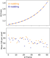 |
Fig. 1 Evolution of the airmass (top panel) and the mean S/N per detector pixel (bottom panel). Data points corresponding to the A and B nodding positions are shown in orange and blue, respectively. |
3 Data reduction
3.1 Extraction of the one-dimensional spectra
We used the CRIRES+ data reduction software pipeline cr2res to extract the one-dimensional spectra from the raw frames2. As a first step, we processed the raw calibration frames taken by the observatory as part of the regular daily calibration routine. These data consist of dark frames, flat fields, and frames taken with a Uranium-Neon lamp and a Fabry-Perot etalon. The calibration data were downloaded from the ESO data archive and reduced using the standard reduction cascade as described in the cr2res pipeline user manual.
We then reduced the science spectra. We grouped the 52 spectra of our time series into 26 pairs of spectra taken at A and B nodding positions. Each nodding pair was reduced using the cr2res_obs_nodding recipe. This procedure applies flat field normalization and bad pixel masking from the calibrations to the raw frames, removes the sky background and instrumental artifacts via subtraction of the A and B frames from each other, and optimally extracts the one-dimensional science spectra and their uncertainties for each wavelength segment.
In general, the wavelength solutions for the A and B spectra calculated by the instrument pipeline are based on observations of a calibration lamp that uniformly illuminates the slit. The wavelength solutions are therefore only accurate if the stellar PSF either fills the slit or is exactly aligned with its center. In our observations, the PSF was smaller than the slit and its position along the dispersion direction was not perfectly centered within the slit, causing an unknown shift of the spectral data points relative to the wavelength solutions of the pipeline. This shift generally differs for the A and B spectra due to the telescope’s nodding motion not being perfectly parallel to the slit orientation of the spectrograph. Therefore, each nodding position had its own wavelength solution.
To account for the shifts in the spectral data points relative to the wavelength solutions of the pipeline, an additional refinement step was applied. We calculated the mean spectrum at each nodding position and applied molecfit (Smette et al. 2015) to the resulting A and B master spectra. By fitting the telluric absorption lines in the master spectra, molecfit corrected the input wavelength solutions by the respective shift and provided us with an improved solution for the A and B spectra as output3. Although the applied procedure results in different molecfit wavelength solutions for A and B, we refrained from shifting the spectral data points to a common wavelength solution to avoid introducing spurious signals during the required interpolation process. Instead, following Yan et al. (2023), we treated the A and B spectra as two independent data sets throughout the subsequent procedures of this section, and combined their information without the need for interpolation in Sects. 4 and 5 after data reduction was complete.
3.2 Pre-processing the spectra
For each wavelength segment, the extracted one-dimensional spectra were sorted chronologically and stacked in a two-dimensional array, yielding a so-called spectral matrix. The baselines of the individual spectra differ from each other due to the variability of the atmospheric conditions during the observations. It is therefore necessary to normalize all spectra to the same continuum level: first, we calculated the median of all spectra in the time series and applied a second-order polynomial fit to the resulting master spectrum. In a second step, all spectra of the spectral matrix were divided by the master and then fitted with a first-order polynomial function. Finally, the continuum correction was obtained as the product of the two previously determined polynomial fit functions and applied by dividing each spectrum.
Outliers were removed using Principal Component Analysis. Using this method, we computed a model of the spectral matrix, subtracted the model from the data, and identified pixels that differed by 5σ from the resulting residuals. The affected pixels were then removed from the spectral matrix. In addition, we masked all wavelength bins with a flux level below 30% of the spectral continuum. We also masked wavelength bins with flux values above 120% of the continuum level to account for strong sky emission lines.
We examined the temporal stability of our molecfit wavelength solution from Sec. 3.1 by cross-correlating each exposure frame with the median spectrum of the time series. Figure 2 shows the radial velocity (RV) drift of the spectra relative to the median for all wavelength segments. The RV drift between the start and end of the observations was less than 0.6 km s−1, with the majority of wavelength segments having even lower drifts on the order of 0.2 km s−1. Both offset values are significantly smaller than a single resolution element of the selected CRIRES+ wavelength setting (~ 2.2 km s−1 at R =135 000). Thus, the molecfit wavelength solution was considered accurate enough for our purposes.
3.3 Removal of telluric and stellar lines
We used the detrending algorithm SYSREM (Tamuz et al. 2005) to correct for the contribution of telluric and stellar lines in the spectral data. Originally designed to identify and remove common signals in light curve studies, the algorithm has demonstrated to be a powerful tool in exoplanet research when applied to high-resolution spectroscopic time series (e.g., Birkby et al. 2013; Nugroho et al. 2017; Sánchez-López et al. 2019).
SYSREM is usually applied over multiple iterations. The algorithm decomposes the contribution of systematic effects to the spectral time series into two column vectors a and c, whose outer product results in a model of the systematics. This model is subtracted from the data, yielding a residual spectral matrix. Based on this residual spectral matrix, a new model with a new set of a and c is calculated. An updated residual spectral matrix is obtained by subtracting the new model from the result of the previous iteration step. The final model of systematic effects after N iterations of SYSREM is thus
![Mathematical equation: $\[\mathbf{M}_{\text {systematic }}=\sum_{k=1}^N \mathbf{a}_k \mathbf{c}_k^T=\mathbf{A} \mathbf{C}^T,\]$](/articles/aa/full_html/2024/08/aa50064-24/aa50064-24-eq6.png) (1)
(1)
where A and C are matrices containing all column vectors ak and ck. Subtracting the model obtained in Eq. (1) from the data yields the final residual spectral matrix, which is used in further analysis steps. We refer the reader to Czesla et al. (2024) for a more detailed mathematical description of SYSREM in the context of exoplanet science.
The input provided to SYSREM includes the pre-processed spectral matrix and the propagated uncertainties from the instrument pipeline. We applied the algorithm following the procedure described by Gibson et al. (2022), which consists of first dividing the spectral matrix by the median spectrum and then subtracting the systematics modeled with SYSREM. This approach allows the distortions of the planet’s signal introduced by the algorithm to be accounted for when a Bayesian retrieval framework is applied to the data in Sec. 5, while preserving the relative strengths of the planetary spectral lines. The uncertainties were propagated by dividing through by the median spectrum. We ran SYSREM for up to ten consecutive iterations and obtained a residual spectral matrix for each iteration and wavelength segment. An overview of the data reduction procedures, including SYSREM, is shown in Fig. 3.
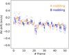 |
Fig. 2 RV drift during the acquisition of the spectral time series. Each data point corresponds to an individual exposure frame and wavelength segment. Data points corresponding to the A and B nodding positions are shown in orange and blue, respectively. |
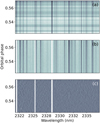 |
Fig. 3 Overview of data reduction procedures for a representative CRIRES+ wavelength range. Panel a: raw spectral matrix after extraction of the one-dimensional spectra. Panel b: spectral matrix after normalization, outlier correction, and masking of the strongest telluric features. Panel c: residual spectral matrix after removal of telluric and stellar lines via two consecutive SYSREM iterations. |
4 Detection of the planetary emission lines
We used the cross-correlation method (e.g., Snellen et al. 2010; Brogi et al. 2012; Birkby et al. 2013) to extract the faint spectral emission lines of WASP-178b from the noise-dominated residual spectra. This method consists of calculating the cross-correlation function (CCF) between an exoplanet model spectrum and the residual spectra, thereby mapping the information of the faint planetary spectral lines onto a detectable signal peak. We searched for the spectral signature of CO, H2O, and OH, which are the chemical species with the most prominent emission lines expected in the K band for any reasonable atmospheric composition. In the specific case of CO, the cross-correlation analysis was performed individually on the molecules with the two isotopologues 12CO and 13CO. In addition, our search included the emission signal of Fe I, which has recently been detected with the same CRIRES+ setting as used in this work in the atmosphere of another UHJ, MASCARA-1b (Ramkumar et al. 2023).
4.1 Model spectra
We considered a planetary atmosphere consisting of 81 layers, equispaced in logarithmic pressure from 10−8 bar to 1 bar. Since the thermal conditions in the dayside atmosphere of WASP-178b have not yet been studied in detail, we adopted the T-p profile measured for KELT-20b/MASCARA-2b (Yan et al. 2022b) to generate the model spectra for a preliminary cross-correlation analysis. Using the T-p profile of this planet is a reasonable approximation because its physical properties are close to those of WASP-178b (e.g., planetary radius, equilibrium temperature, orbital period, host star type). By applying the cross-correlation method described in Sec. 4.2, we obtained a significant detection of the 12CO and H2O emission lines. We then used the retrieval framework detailed in Sec. 5, which allowed us to determine the best-fit T-p profile of WASP-178b’s dayside atmosphere. The best-fit atmospheric profile was used to generate the final model spectra, which yielded the cross-correlation analysis results described below.
The T-p profile is parametrized by a low pressure point (T1, p1) and a high pressure point (T2, p2), with an isothermal atmosphere at pressures below p1 or higher than p2 (Fig. 4). The temperature between the two isothermal layers was assumed to change linearly as a function of log p. Assuming equilibrium chemistry and the elemental abundances (Asplund et al. 2009) retrieved in Sec. 5, we used FastChem (Stock et al. 2018)4 to obtain the mean molecular weight and volume mixing ratio (VMR) of the chemical species studied (Fig. 4). In addition, for each chemical species we needed a T-p-wavelength grid of its opacities to calculate the corresponding model spectrum. The data used to compute the high-resolution opacities were obtained from the following sources: CO line information from Li et al. (2015), H2O data from the POKAZATEL line list (Polyansky et al. 2018), OH opacities from the MoLLIST database (Brooke et al. 2016), Fe I atomic line data from Kurucz (2018). We ran the radiative transfer code petitRADTRANS (Mollière et al. 2019) to generate the high-resolution model spectra of the different chemical species (R = 106). Finally, the resulting model spectra were convolved with the rotational broadening profile described in Sec. 5.
During the pre-processing steps of our analysis, the spectra were normalized to the continuum level. Thus, our model spectra also required continuum normalization. As a first step, we divided each spectral model by the blackbody spectrum of the host star. The resulting planet-to-star flux ratio was then normalized to the planetary continuum and convolved with the instrumental profile, yielding the final model spectra for cross-correlation. The normalized model spectra of all studied chemical species are shown in Figs. 5 and 6.
4.2 Cross-correlation method
We used the cross-correlation technique to study each chemical species independently. The model spectrum was Doppler-shifted to a grid of velocities between −800 km s−1 and +800 km s−1, with a cadence of 1 km s−1. We multiplied the shifted model spectrum of each grid point by the uncertainty-weighted residual spectra, resulting in a so-called weighted CCF for each exposure frame. For the residual spectrum number i of the time series, the CCF is thus defined as
![Mathematical equation: $\[\mathrm{CCF}_i(v)=\sum_j \frac{R_{i j} m_j(v)}{\sigma_{i j}{ }^2},\]$](/articles/aa/full_html/2024/08/aa50064-24/aa50064-24-eq7.png) (2)
(2)
with Rij being the matrix of residual spectra, σij the corresponding uncertainties, and mj the spectral model shifted by the Doppler-velocity υ. For each wavelength segment, the CCFs of the spectral time series were arranged in a two-dimensional array. The arrays of the different wavelength segments were then co-added, resulting in a CCF map for each of the A and B spectral subsets. Eventually, the CCF maps of the two nodding positions were combined into a final CCF map for the individual spectral models.
The CCF map was aligned to the rest frame of WASP-178b over a range of different orbital semi-amplitude velocity (Kp) values. For this purpose, we assumed a circular planetary orbit, whose radial velocity is described by
![Mathematical equation: $\[v_{\mathrm{p}}(t)=v_{\text {sys }}+v_{\text {bary }}(t)+K_{\mathrm{p}} \sin 2 \pi \phi(t),\]$](/articles/aa/full_html/2024/08/aa50064-24/aa50064-24-eq8.png) (3)
(3)
where υsys is the systemic velocity, υbary (t) is the barycentric velocity correction, and ϕ (t) is the orbital phase. Each shifted CCF map was then collapsed into a one-dimensional CCF by averaging over all orbital phases. The one-dimensional CCF of each alignment was further stacked into a two-dimensional array. To quantify the noise level of the array as objectively as possible, we fit the distribution of all CCF values with a Gaussian function (e.g., Brogi et al. 2023). After dividing the array with the standard deviation of the Gaussian, we obtained a signal-to-noise detection map (S/N map) as a function of Kp and υsys. If the signature of the investigated chemical species is present in the planetary spectrum, a significant detection peak will appear at the expected values of Kp and υsys in the S/N map.
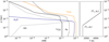 |
Fig. 4 Volume mixing ratios (VMRs; left panel) and T-p profile (right panel) used to generate the model spectra for cross-correlation. The VMRs were calculated assuming equilibrium chemistry. The elemental abundances and the T-p profile used correspond to the best-fit results of the retrieval framework in Sec. 5. |
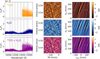 |
Fig. 5 Spectral models, CCF maps, and S/N maps of 12CO, H2O, and both species together. The left panels show the continuum normalized model spectra. Wavelengths covered by the CRIRES+ K2166 setting used in this work are indicated by the gray shaded area. The middle panels illustrate the CCF maps. The spectral signal from WASP-178b’s atmosphere can be identified as a diagonal trail. The expected RV evolution as a function of orbital phase is indicated by the yellow dashed lines. The right panels show the S/N maps. The expected position of the planetary signal is indicated by the yellow dashed lines. We show the CCF maps and S/N maps corresponding to two consecutive runs of SYSREM, which is the number of iterations used in the retrieval in Sec. 5. |
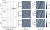 |
Fig. 6 Same as Fig. 5, but for 13CO, OH, and Fe I. These species result in non-detections due to the weakness and low number of spectral lines over the investigated wavelength range. The CCF maps and S/N maps are the result of two consecutive SYSREM iterations. |
4.3 Cross-correlation results and discussion
We significantly detect spectral emission lines from the dayside atmosphere of WASP-178b. Figure 5 shows the CCF maps and S/N maps from the cross-correlation of our data with the 12CO, H2O, and the species-combined model spectra. The dashed lines indicate the expected location of the planetary signal in the maps as computed from the parameters of Rodríguez Martínez et al. (2020). For all SYSREM iterations larger than one, both chemical species present a clearly visible CCF trail and a S/N detection peak close to the predicted values of Kp and υsys. We find the strongest detection of the 12CO spectral signature with S/N = 8.9 after two SYSREM iterations; the most prominent H2O signal is achieved with S/N = 4.9 after five consecutive runs of SYSREM. Cross-correlation with a model spectrum including the spectral lines of both chemical species yields a maximum detection after two SYSREM iterations with S/N = 8.8. Comparison of this detection strength with the S/N values of the individual species shows that the spectral signature of 12CO dominates the combined signal. This finding is reasonable considering the increased thermal stability of 12CO compared to H2O, resulting in higher abundances and stronger spectral lines of this species (Figs. 4 and 5). The detection strengths, signal positions, as well as the noise pattern in the S/N maps of both chemical species show a stable pattern for all SYSREM iterations larger than one. We show the evolution of the detection strengths as a function of SYSREM iterations in Fig. 7. The detection of spectral lines in emission shape unambiguously proves the presence of an atmospheric temperature inversion in the dayside of WASP-178b, consistent with theoretical predictions on the thermal structure of UHJ atmospheres (e.g., Hubeny et al. 2003; Fortney et al. 2008).
Figure 8 illustrates a detailed view of the one-sigma regions around the 12CO and H2O detection peaks. The signals of the two species show an offset in the order of a few km s−1 in Kp-υsys space relative to each other, with only a marginal overlap. The different Doppler-shifts prevent a constructive addition of the 12CO and H2O signals in the S/N map in Fig. 5, explaining the species-combined detection strength being slightly lower than that of 12CO alone. The 12CO signal is inconsistent, that of H2O is consistent with the expected orbital parameter values. This is not the first time that signals from different chemical species have been found to have deviating Doppler-shifts. For example, recent observations of the UHJ WASP-18b have revealed a similar effect for the spectral emission lines of CO, H2O, and OH with comparable amplitude in both Kp and υsys (Brogi et al. 2023). In addition, a significant offset between the signatures of Fe I and TiO was identified in the dayside emission spectrum of WASP-33b (Cont et al. 2021). Transmission spectroscopy of gas giant exoplanets has also shown the existence of significant offsets between the detection coordinates in the S/N maps of individual chemical species (e.g., Kesseli et al. 2022; Sánchez-López et al. 2022a). We rule out calibration inaccuracies as a possible cause for the observed offset between the 12CO and H2O signals, since the precision of our molecfit wavelength solution is below the size of a single resolution element of the instrument. Furthermore, the offsets are unlikely to be caused by the line lists used, since previous high-resolution spectroscopy studies have been able to detect 12CO and H2O simultaneously without detecting a significant Doppler-shift between the two chemical species (e.g., Holmberg & Madhusudhan 2022; Ramkumar et al. 2023). In addition, the results of Gandhi et al. (2020) suggest the suitability of the 12CO and H2O line lists to study exoplanet atmospheres.
Offsets between the signatures of individual chemical species in Kp-υsys space may indicate a difference in the local “slope” of the Keplerian radial velocity curve, caused by atmospheric circulation and chemical inhomogeneity effects (Brogi et al. 2023). The concentration of 12CO decreases significantly slower than that of H2O towards lower pressure values (Fig. 4). Consequently, the emission lines of the two species are expected to probe different pressure regimes in WASP-178b’s atmosphere. Doppler-offsets between the individual chemical species may therefore be caused by differences in the dynamics of the respective atmospheric layers. In addition, chemical inhomogeneities across WASP-178b’s surface, in combination with the planetary rotation, have the potential to add an individual Doppler-shift to the signature of each chemical species. While the existence of an offset between the measured 12 CO peak and the expected Kp-υsys coordinates is confidently detected, we emphasize that caution is required in interpreting the position of the weaker H2O signal in the S/N map. The one-sigma region of the species extends over a wide range of orbital parameter values, making it difficult to draw precise conclusions about the Doppler-shift of the signal. In addition, the relatively low signal strength raises the possibility that the observed position in Kp-υsys space could be affected by distortion of the H2O peak due to the intrinsic noise pattern of the S/N map. Future observations will provide a stronger H2O signal, improving the ability to study the three-dimensional structure and dynamics of WASP-178b’s atmosphere.
Figure 6 shows the S/N maps of 13CO, OH, and Fe I. No significant detections are found in the S/N maps of the three chemical species. We conducted an injection-recovery test to validate our findings. In a first step, we Doppler-shifted the convolved model spectra used to attempt the detection of the chemical species with the reversed Kp value of −176.5 km s−1 (Merritt et al. 2020; Cont et al. 2022a). The shifted spectral models were then injected into the raw data, and the pre-processing and cross-correlation analyses were performed as described in Sects. 3 and 4. Doppler-shifting the injected signal with the negative Kp of WASP-178b serves to avoid interference with potentially undetected planetary emission lines of the investigated chemical species. None of the injected signals were recovered (Fig. 9). The nondetections of the chemical species 13CO, OH, and Fe I are therefore most likely due to the limited number and low intensity of their spectral emission lines in the wavelength range studied, rather than to their absence in the planetary atmosphere. In fact, OH emission lines were identified in the spectra of gas giant exoplanets other than WASP-178b, but blueward of the wavelength range analyzed in this work (e.g., Nugroho et al. 2021; Brogi et al. 2023). In addition, Fe I lines have commonly been identified at visible wavelengths in the spectra of UHJs (e.g., Pino et al. 2022; Yan et al. 2022b). The emission signature of 13CO has also been detected at near-infrared wavelengths by Zhang et al. (2021), albeit by medium-resolution spectroscopy for a gas giant at a significantly larger orbital separation compared to UHJs.
 |
Fig. 7 S/N values as a function of SYSREM iterations. We show the detection strengths obtained from cross-correlation with model spectra including the emission lines of 12CO, H2O, and both species together, respectively. The iteration with the most significant S/N peak is indicated by the star symbol. In our retrieval framework in Sec. 5, we used the iteration number that yields the most prominent S/N detection peak of the species-combined signal, i.e., two consecutive SYSREM iterations. |
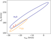 |
Fig. 8 One-sigma regions of 12CO and H2O detections. The position of the 12CO signal is inconsistent, that of the H2O signal is consistent with the expected Kp and υsys values, whose location is indicated by the red symbols (“+”: Hellier et al. 2019; “×”: Rodríguez Martínez et al. 2020). |
5 Retrieval of the atmospheric properties
Retrieval frameworks allow the derivation of statistical constraints on the physical and chemical parameters of exoplanet atmospheres by comparing a parameterized model spectrum with observational data. In this study, we adopt the approach previously used by Yan et al. (2023) and Lesjak et al. (2023) to quantitatively assess the atmospheric conditions of WASP-178b. This framework is an evolution of the retrieval method introduced by Yan et al. (2020), inspired by Brogi & Line (2019), Shulyak et al. (2019), and Gibson et al. (2020), and successfully used in previous work on UHJs (Yan et al. 2022b; Cont et al. 2022a; Borsa et al. 2022). The main advancement in this retrieval is the integration of a method that accounts for potential distortions in the spectral data introduced by SYSREM.
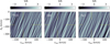 |
Fig. 9 S/N maps of injection-recovery test. The yellow dashed lines indicate the coordinates of the injected signal. The injected signatures of 13CO, OH, and Fe I could not be identified, indicating that even if present in the planetary atmosphere, these species are undetectable. |
5.1 Retrieval framework
5.1.1 High-resolution retrieval
We used the radiative transfer code petitRADTRANS (Mollière et al. 2019) to forward model the emission spectrum of WASP-178b (R = 106). Our radiative transfer calculations included the opacities of the detected chemical species 12CO and H2O, as well as those of H−, which has been suggested as an important continuum source capable of muting emission features in the spectra of UHJs (e.g., Arcangeli et al. 2018; Lothringer et al. 2018). The use of petitRADTRANS requires the definition of the thermal and chemical properties of the investigated planetary atmosphere. For this purpose, we modeled the atmosphere of WASP-178b with 25 layers uniformly distributed on a logarithmic scale between 10−8 bar and 1 bar. The reduced number of atmospheric layers compared to those used to generate the spectral models in Sec. 4.1 allows us to speed up our radiative transfer calculations. We have verified that the number of layers used has a negligible impact on the accuracy of the calculated model spectra (Fig. 10). As outlined in Sec. 4.1, a two-point T-p parametrization was used to describe the thermal profile of the atmosphere. Instead of using the high pressure point p2 directly, we define it as log p2 = log p1 + dp. We limited dp to positive values to ensure that p2 has a value higher than p1. The chemical equilibrium code FastChem (Stock et al. 2018) was employed to calculate the VMRs as a function of the atmospheric metallicity ([M/H]) and C/O ratio. To account for the non-negligible effect of WASP-178b’s rotation, we convolved the petitRADTRANS forward model with a broadening profile parametrized by the planetary equatorial rotation velocity υeq. The analytical expression of the broadening profile is given in Eq. (3) of Díaz et al. (2011) and has been commonly used to study stellar rotation. We assumed a limb darkening coefficient of ϵ = 1, corresponding to a flux contribution tending to zero towards the planetary limb. In addition, the inclination angle of WASP-178b’s equator was set to the same value as the orbital inclination angle of the planet, under the hypothesis of a tidally locked rotation. The model spectrum was further converted to the planet-to-star flux ratio and convolved with the instrumental profile as described in Sec. 4.1.
We Doppler-shifted the model spectrum to the radial velocity of each exposure frame of our spectral time series. The shift was calculated using Eq. (3), thus depending on the values of Kp and υsys. We interpolated each Doppler-shifted model spectrum to the wavelength solution of the observational data points and arranged the resulting one-dimensional vectors in a two-dimensional array. This procedure yielded a two-dimensional forward model matrix, with the same shape as the residual spectral matrix.
The presence of distortion effects on the spectral emission lines introduced by SYSREM was incorporated into the forward model matrix. To this end, we adopted the filtering method proposed by Gibson et al. (2022), which avoids the time-consuming application of SYSREM to the two-dimensional forward model at each sampling step of the retrieval. This technique consists of applying the filter
![Mathematical equation: $\[\mathbf{F}=\mathbf{A}(\boldsymbol{\Lambda} \mathbf{A})^{\dagger}\left(\boldsymbol{\Lambda} \mathbf{M}_{\text {unfiltered }}\right)\]$](/articles/aa/full_html/2024/08/aa50064-24/aa50064-24-eq9.png) (4)
(4)
to the unfiltered forward model matrix Munfiltered. The matrix A is defined in Sect. 3.3, Λ is a diagonal matrix containing the inverse of the mean uncertainties in wavelength direction, and X† = (XTX)−1 XT denotes the Moore-Penrose inverse of a matrix X. We pre-calculated and applied the filter to each model during the retrieval, resulting in a filtered model matrix M = Munfiltered − F, which was compared to the data.
A standard Gaussian log likelihood function
![Mathematical equation: $\[\ln L=-\frac{1}{2} \sum_{i, j}\left[\frac{\left(R_{i j}-M_{i j}\right)^2}{\left(\beta \sigma_{i j}\right)^2}+\ln 2 \pi\left(\beta \sigma_{i j}\right)^2\right]\]$](/articles/aa/full_html/2024/08/aa50064-24/aa50064-24-eq10.png) (5)
(5)
was defined to compare each generated forward model with the residual spectra. In this expression, Rij and Mij denote the individual elements of the residual spectral matrix and the filtered forward model matrix, respectively. The uncertainties of the residual spectra are represented by σij, while β acts as a scaling factor to correct for possible over- or underestimation of the uncertainties. We used the residual spectral matrix that gives the most prominent S/N detection peak, which was obtained after two consecutive SYSREM iterations (see Fig. 7). To confirm that our choice of the iteration number has no significant effect on the retrieval result, we repeated our calculations with the spectral matrices from SYSREM iterations other than the optimal number of two consecutive runs, for which we did not find any significant differences. For each wavelength segment and nodding position, the log likelihood function was calculated independently, and the resulting values were summed to obtain the combined log likelihood function of all data. To estimate the model parameters, we evaluated the combined log likelihood function by Markov Chain Monte Carlo (MCMC) sampling using the emcee software package (Foreman-Mackey et al. 2013).
In summary, our high-resolution retrieval framework includes the following free parameters: the temperature profile parameters T1, p1, T2, dp; the chemical properties represented by [M/H] and the C/O ratio; the equatorial rotation velocity υeq; the velocity parameters Kp and υsys; the noise scaling parameter β. For each free parameter, we used 32 walkers with 15000 steps in the sampling.
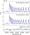 |
Fig. 10 Comparison between model spectra computed with 25 (top panel) and 81 (middle panel) atmospheric layers. The model spectra include the opacities of the detected chemical species 12CO and H2O, as well as those of H−. The difference between the models is insignificant (bottom panel), implying that the lower number of atmospheric layers does not significantly affect our retrieval results. |
5.1.2 Joint retrieval with photometric data
High-resolution spectroscopy observations lack the information from the spectral continuum level, which is lost when correcting for the telluric and stellar lines with SYSREM. Therefore, only the relative strengths of the spectral lines with respect to the local continuum can be measured, reducing the reliability of retrievals when relying solely on high-resolution spectroscopy. On the other hand, space-based observations can measure absolute flux levels that encode the spectral continuum information of exoplanet atmospheres. An analysis that combines our highresolution CRIRES+ data with space-based measurements will therefore improve the robustness of our retrieval results.
Recently, Pagano et al. (2023) measured the secondary eclipse depth of WASP-178b using space-based photometry with TESS and CHEOPS, obtaining eclipse depth values of 70±20 ppm and 70±40 ppm, respectively. We incorporated these two photometric data points into our retrieval framework using an approach similar to that proposed by Yan et al. (2022b), which we complemented by including the reflection of stellar light by the planetary atmosphere. Given the photometric passband η(λ), this approach models the eclipse depth as
![Mathematical equation: $\[\delta_{\mathrm{ecl}}=A_{\mathrm{g}}\left(\frac{R_{\mathrm{p}}}{a}\right)^2+\left(\frac{R_{\mathrm{p}}}{R_*}\right)^2 \frac{\int \eta~(\lambda) ~F_{\mathrm{p}}~(\lambda) ~\mathrm{d} \lambda}{\int \eta~(\lambda) ~F_*(\lambda) ~\mathrm{d} \lambda},\]$](/articles/aa/full_html/2024/08/aa50064-24/aa50064-24-eq11.png) (6)
(6)
where Ag is the geometric albedo, a is the orbital separation of the planet-star system, and Rp and R* are the planetary and stellar radii. Additionally, Fp (λ) and F* (λ) represent the fluxes originating from the planetary and stellar atmospheres per unit area and per unit wavelength. The first term of this expression accounts for the contribution of the stellar light reflected by the planetary atmosphere; the second term represents the thermal emission contribution to the planet-to-star flux ratio integrated over the instrumental passband.
We used petitRADTRANS to calculate the thermal emission component of Eq. (6) over the wavelength range of TESS and CHEOPS. The photometric bandpasses of both instruments cover a significant fraction of the visible wavelength range where strong emission lines of atomic metals, their oxides, and hydrides are expected. In our radiative transfer calculations, we included the opacities of Fe, Ti, Na, K, Ca, Mg, TiO, VO, FeH, CrH, and CaH, which represent the metal species with the most prominent emission features at visible wavelengths for any reasonable atmospheric composition (e.g., Hubeny et al. 2003; Fortney et al. 2008; Lothringer & Barman 2019). Additionally, we accounted for the contribution from the continuum opacity source H−. We provided petitRADTRANS with the same thermal and chemical parametrizations as detailed in Sect. 5.1.1. The resulting emission flux of each instrument was integrated over its respective bandpass using the rebin-give-width tool of petitRADTRANS. We integrated over the range 0.60 to 1.00 μm for TESS, while for CHEOPS the integration was performed over the range 0.35 to 1.10 μm. Since the model spectrum was integrated over the relatively wide TESS and CHEOPS bandpasses, we used the petitRADTRANS low-resolution mode to speed up the radiative transfer calculations. The opacities used in the low-resolution mode require less dense sampling in wavelength space than those used to generate the high-resolution CRIRES+ model spectra, and are available in the petitRADTRANS opacity database5.
We then defined the log likelihood function for the photometric data. For a specific eclipse depth measurement, this function is given by
![Mathematical equation: $\[\ln L_{\mathrm{ecl}}=-\frac{1}{2}\left[\frac{\left(R_{\mathrm{ecl}}-\delta_{\mathrm{ecl}}\right)^2}{\sigma_{\mathrm{ecl}}^2}+\ln 2 \pi \sigma_{\mathrm{ecl}}^2\right],\]$](/articles/aa/full_html/2024/08/aa50064-24/aa50064-24-eq12.png) (7)
(7)
where Recl is the photometric eclipse depth measurement, δecl is the model of the eclipse depth, and σecl is the measurement uncertainty. We calculated the log likelihood functions for both the TESS and CHEOPS data points. We then added these functions to the combined log likelihood function of the highresolution data described in Sect. 5.1.1. The resulting final log likelihood function incorporates all the information from the high-resolution and photometric data. We performed the joint retrieval on the CRIRES+, TESS, and CHEOPS data by evaluating the final log likelihood function via MCMC sampling. In addition to the free parameters outlined in Sect. 5.1.1, the retrieval incorporates the geometric albedo Ag. We set Ag as gray albedo, which assumes wavelength independence. For each free parameter, 32 walkers with 15 000 steps each were used in the MCMC sampling process.
Results of atmospheric retrievals on WASP-178b.
5.2 Results and discussion
5.2.1 High-resolution retrieval
In a first step, we applied the retrieval only to the high-resolution spectroscopy data obtained from CRIRES+. The corner plot in Fig. A.1 shows the resulting posterior distributions along with the correlations of the atmospheric parameters. A summary of the best-fit retrieval parameters is provided in Table 3. The noise scaling term β is close to one, indicating an appropriate estimation of the uncertainties.
The retrieval confirms the presence of the inverted atmospheric T-p profile detected in Sec. 4. Figure A.1a shows examples of the T-p profiles sampled by the MCMC analysis, and Fig. A.1b illustrates the median temperature curve. The thermal inversion layer spans the pressure range from approximately 10−5 bar to 1 bar, with temperatures of T1 > 3700K and T2 < 2800 K in the upper and lower planetary atmosphere, respectively. The strength of the atmospheric temperature inversion is consistent with both theoretical predictions (Hubeny et al. 2003; Fortney et al. 2008; Arcangeli et al. 2018) and previous observational studies of UHJs with system architectures similar to WASP-178b (e.g., Yan et al. 2020, 2022b).
Although we are able to infer the existence of a strong thermal inversion, our retrieval is not able to precisely capture the physical conditions in the uppermost layers of WASP-178b’s atmosphere. This can be seen when considering the posterior distribution of the temperature parameter T1 in Fig. A.1, which parametrizes the upper boundary of the thermal inversion layer. In particular, at high values of T1, the posterior probability distribution of the parameter tends to have a flat pattern. In the context of Bayesian retrieval frameworks, such a flat posterior distribution generally indicates a lack of information from the observational data in the specific parameter range. The presence of little spectral information from the upper planetary atmosphere is indeed expected, since 12CO and H2O generally undergo strong dissociation with decreasing atmospheric pressure. Consequently, the spectral emission signature of 12CO and H2O will originate primarily from atmospheric layers where higher pressures allow significant abundances of the two molecular species to persist.
Similar to T1, the retrieval on the CRIRES+ data can barely constrain the temperature parameter T2, which describes the lower boundary of the thermal inversion layer. The posterior probability distribution of T2 flattens towards lower values, suggesting that limited information can be recovered in this temperature range. We attribute the poor constraints on T2 to the absence of information from the spectral continuum level, which encodes the physical properties at the bottom of the thermal inversion layer but was removed from the data during the correction for systematic effects in Sec. 3.3. The absence of information on the spectral continuum level also explains the degeneracy between T2 and p2, which leads to large uncertainties in the value of p2. Given the weak constraints on T2 and p2, several of the sampled thermal inversions in Fig. A.1a extend to temperatures below 1000 K and pressures well above 1 bar. These temperature values are not plausible given the extreme thermal conditions in UHJ atmospheres, while the elevated pressure values correspond to atmospheric layers inaccessible to spectral observations. In summary, we are unable to accurately measure both the upper and lower boundaries of the thermal inversion layer using high-resolution CRIRES+ data alone.
Our retrieval constrains the atmospheric metallicity to ![Mathematical equation: $\[[\mathrm{M} / \mathrm{H}]=0.40_{-0.99}^{+1.81}\]$](/articles/aa/full_html/2024/08/aa50064-24/aa50064-24-eq29.png) dex, which is in agreement with the host star value of
dex, which is in agreement with the host star value of ![Mathematical equation: $\[-0.06_{-0.34}^{+0.30}\]$](/articles/aa/full_html/2024/08/aa50064-24/aa50064-24-eq30.png) dex (Rodríguez Martínez et al. 2020). In addition, we derived an upper limit for the atmospheric C/O ratio of 0.84, which is consistent with the solar value of 0.55. A degeneracy of the measured [M/H] with the pressure parameters p1 and p2, as well as between the C/O ratio and p2, is indicated by the diagonal distribution patterns in the correlation plots of Fig. A.1. Under the hypothesis of equilibrium chemistry, the concentrations of 12CO and H2O decrease in the upper planetary atmosphere due to the growing influence of molecular dissociation towards lower pressures. The effect of the reduced molecular concentrations on the forward model spectrum can be counterbalanced by increasing the [M/H] value, explaining the degeneracy between the pressure parameters and [M/H]. In addition, the concentration of H2O decreases faster than that of 12CO in the low pressure regime. The influence of the lower H2O concentration on the spectral forward model can be compensated by decreasing the C/O ratio, resulting in the observed degeneracy with the pressure parameter. Consequently, uncertainties in the retrieved T-p profile have the potential to critically affect the [M/H] and C/O values. More precise constraints on the T-p profile will be derived in Sect. 5.2.2, improving the reliability of the parameters that describe the atmospheric chemistry.
dex (Rodríguez Martínez et al. 2020). In addition, we derived an upper limit for the atmospheric C/O ratio of 0.84, which is consistent with the solar value of 0.55. A degeneracy of the measured [M/H] with the pressure parameters p1 and p2, as well as between the C/O ratio and p2, is indicated by the diagonal distribution patterns in the correlation plots of Fig. A.1. Under the hypothesis of equilibrium chemistry, the concentrations of 12CO and H2O decrease in the upper planetary atmosphere due to the growing influence of molecular dissociation towards lower pressures. The effect of the reduced molecular concentrations on the forward model spectrum can be counterbalanced by increasing the [M/H] value, explaining the degeneracy between the pressure parameters and [M/H]. In addition, the concentration of H2O decreases faster than that of 12CO in the low pressure regime. The influence of the lower H2O concentration on the spectral forward model can be compensated by decreasing the C/O ratio, resulting in the observed degeneracy with the pressure parameter. Consequently, uncertainties in the retrieved T-p profile have the potential to critically affect the [M/H] and C/O values. More precise constraints on the T-p profile will be derived in Sect. 5.2.2, improving the reliability of the parameters that describe the atmospheric chemistry.
High-resolution spectroscopy retrievals in the literature typically assume constant VMRs, rather than allowing abundances to vary with atmospheric altitude (e.g., Gandhi et al. 2023; Yan et al. 2023). To better capture the chemical conditions as a function of atmospheric pressure, equilibrium chemistry calculations can be incorporated into retrieval frameworks (e.g., Madhusudhan & Seager 2009; Line et al. 2012; Kitzmann et al. 2020). We note that the equilibrium chemistry approximation is not generally valid over the entire pressure and temperature range of exoplanet atmospheres, as chemical disequilibrium effects can alter the VMRs of different chemical species (e.g., Shulyak et al. 2020). However, theoretical work has also shown that in the specific case of temperatures in the UHJ regime, the assumption of equilibrium chemistry may be a valid approximation (Kitzmann et al. 2018).
In contrast to the somewhat weak constraints on the thermal structure and chemical conditions, our retrieval is able to obtain tight confidence intervals for the planetary parameters encoded in the Doppler-shifts and the width of the spectral emission lines. We retrieve the orbital and systemic velocity parameters with high precision as ![Mathematical equation: $\[K_{\mathrm{p}}=174.46_{-6.44}^{+7.22} \mathrm{~km} \mathrm{~s}^{-1}\]$](/articles/aa/full_html/2024/08/aa50064-24/aa50064-24-eq31.png) and
and ![Mathematical equation: $\[v_{\text {sys }}=-23.26_{-1.89}^{+2.03} \mathrm{~km} \mathrm{~s}^{-1}\]$](/articles/aa/full_html/2024/08/aa50064-24/aa50064-24-eq32.png) . These velocity values are in line with the location of the S/N detection peak obtained via cross-correlation with the combined model of 12CO and H2O in Sec. 4. The derived value of υsys is in agreement with the measurement reported by Hellier et al. (2019), while a slight blue-shift is found with respect to the result of Rodríguez Martínez et al. (2020). Such a blue-shift can generally indicate a net flow of atmospheric gas towards the observer. This phenomenon has allowed the identification of day-to-nightside winds in the atmospheres of several exoplanets via transmission spectroscopy (e.g., Snellen et al. 2010; Alonso-Floriano et al. 2019). Our emission spectroscopy observations, however, correspond to orbital phases close to the secondary eclipse. In this observation geometry, a blue-shifted spectral signal would result from a net material flow from the nightside to the dayside, a dynamical regime not predicted by global circulation models of UHJs (e.g., Showman et al. 2013; Tan & Komacek 2019). Therefore, and given the agreement between our υsys value and that of Hellier et al. (2019), we suggest that the small offset from the Rodríguez Martínez et al. (2020) measurement is unlikely caused by global winds in WASP-178b’s atmosphere. Overall, the inconsistency between the results of the two detection papers of WASP-178b makes it difficult to interpret our υsys measurement in absolute terms. However, the offset does not affect our interpretation of the relative Doppler-shift between the 12CO and H2O emission lines discussed in Sec. 4.
. These velocity values are in line with the location of the S/N detection peak obtained via cross-correlation with the combined model of 12CO and H2O in Sec. 4. The derived value of υsys is in agreement with the measurement reported by Hellier et al. (2019), while a slight blue-shift is found with respect to the result of Rodríguez Martínez et al. (2020). Such a blue-shift can generally indicate a net flow of atmospheric gas towards the observer. This phenomenon has allowed the identification of day-to-nightside winds in the atmospheres of several exoplanets via transmission spectroscopy (e.g., Snellen et al. 2010; Alonso-Floriano et al. 2019). Our emission spectroscopy observations, however, correspond to orbital phases close to the secondary eclipse. In this observation geometry, a blue-shifted spectral signal would result from a net material flow from the nightside to the dayside, a dynamical regime not predicted by global circulation models of UHJs (e.g., Showman et al. 2013; Tan & Komacek 2019). Therefore, and given the agreement between our υsys value and that of Hellier et al. (2019), we suggest that the small offset from the Rodríguez Martínez et al. (2020) measurement is unlikely caused by global winds in WASP-178b’s atmosphere. Overall, the inconsistency between the results of the two detection papers of WASP-178b makes it difficult to interpret our υsys measurement in absolute terms. However, the offset does not affect our interpretation of the relative Doppler-shift between the 12CO and H2O emission lines discussed in Sec. 4.
In addition, our retrieval reveals the presence of significant spectral line broadening. Assuming that broadening of the spectral emission lines is mainly caused by the planetary rotation, we derive an equatorial rotation velocity of ![Mathematical equation: $\[v_{\text {eq }}=5.65_{-1.13}^{+1.17} \mathrm{~km} \mathrm{~s}^{-1}\]$](/articles/aa/full_html/2024/08/aa50064-24/aa50064-24-eq33.png) . We exclude that thermal or pressure broadening cause the increased width of the spectral line profile, since these effects are already included in the forward model via the opacities of the radiative transfer calculation. We also rule out that smearing of the spectral signal over multiple pixels due to the wavelength shift during the observations causes the broadened line profile. The 240 s exposure time of each spectrum corresponds to a smearing slightly less than 1 km s−1, which is significantly below the size of a single CRIRES+ resolution element. The derived υeq is significantly higher than that expected from a tidally locked rotation of WASP-178b, which would yield a value of ~ 3 km s−1. This finding indicates the presence of strong atmospheric dynamics, most likely global-scale winds flowing parallel to the equator in the same direction as the planetary rotation. Indeed, global circulation models predict the existence of super-rotating winds in the atmospheres of gas giant exoplanets (e.g., Showman et al. 2009; Heng et al. 2011; Beltz et al. 2021).
. We exclude that thermal or pressure broadening cause the increased width of the spectral line profile, since these effects are already included in the forward model via the opacities of the radiative transfer calculation. We also rule out that smearing of the spectral signal over multiple pixels due to the wavelength shift during the observations causes the broadened line profile. The 240 s exposure time of each spectrum corresponds to a smearing slightly less than 1 km s−1, which is significantly below the size of a single CRIRES+ resolution element. The derived υeq is significantly higher than that expected from a tidally locked rotation of WASP-178b, which would yield a value of ~ 3 km s−1. This finding indicates the presence of strong atmospheric dynamics, most likely global-scale winds flowing parallel to the equator in the same direction as the planetary rotation. Indeed, global circulation models predict the existence of super-rotating winds in the atmospheres of gas giant exoplanets (e.g., Showman et al. 2009; Heng et al. 2011; Beltz et al. 2021).
In principle, the signature of a super-rotating atmosphere should be observable either as a Doppler-shift (Seidel et al. 2023) or as a bi- or trimodal profile (Nortmann et al. 2024) of the spectral lines during primary eclipses. Recent transmission spectroscopy observations of WASP-178b at visible wavelengths with ESPRESSO have revealed the absence of such a signature in the absorption lines of atomic metals (Damasceno et al. 2024). Localized zonal winds on the dayside of WASP-178b that dissipate before reaching the terminator could provide an explanation for both the ESPRESSO transmission and CRIRES+ emission spectroscopy observations. Such an atmospheric flow pattern has recently been proposed by Seidel et al. (2023) to explain the absence of a jet stream near the terminators of the UHJ WASP-121b. Alternatively, a bi- or trimodal line profile could be present, but not resolved in the ESPRESSO transmission observations. Future transmission and emission spectroscopy observations over an extended wavelength range and orbital phase interval are needed to improve our understanding of the atmospheric circulation in WASP-178b’s dayside.
5.2.2 Joint retrieval with photometric data
In a next step, we performed the retrieval that includes both the high-resolution spectroscopy data from CRIRES+ and the photometric measurements from TESS and CHEOPS. The corner plot in Fig. A.2 illustrates the resulting posterior distributions and the correlations between the atmospheric parameters. A comparison with the posterior probability distributions of the high-resolution retrieval is shown in Fig. 11. The best-fit parameters are summarized in Table 3. All retrieval parameters except the newly introduced geometric albedo Ag agree with the results of the high-resolution retrieval within the uncertainty intervals.
The atmospheric T-p profiles obtained from the MCMC sampling process are shown in Fig. A.2a, while the median temperature profile is reported in Fig. A.2b. Analogous to the high-resolution retrieval in Sect.5.2.1, the posterior distribution of the temperature parameter T1 flattens towards higher values, resulting in a lower limit on the parameter at T1 > 3200 K. This finding is in line with our expectations, since space-based photometry provides little additional information about the physical conditions in the upper atmospheric layers of gas giant exoplanets.
The refined constraints on the temperature limit at the bottom of the atmospheric inversion layer of T2 < 2000 K are a direct consequence of the inclusion of the TESS and CHEOPS data, which encode the spectral continuum level information from the lower planetary atmosphere. Our improved ability to probe the low-altitude boundary of the thermal inversion is also reflected in the disappearance of the degeneracy between the temperature and pressure parameters T2 and p2. This allows us to measure the thermal properties of the atmosphere more accurately than with high-resolution data alone. Breaking this degeneracy slightly lowers p2, shifting the measured thermal inversion layer to higher atmospheric altitudes. This shift can be seen in Fig. 12, which compares the T-p profiles derived from the high-resolution retrieval and the joint retrieval with TESS and CHEOPS.
The metallicity of ![Mathematical equation: $\[[\mathrm{M} / \mathrm{H}]=1.39_{-1.58}^{+1.64}\]$](/articles/aa/full_html/2024/08/aa50064-24/aa50064-24-eq34.png) dex obtained from the joint retrieval is higher than that based on the analysis of the high-resolution observations alone. However, given the relatively large uncertainty intervals, the result is still consistent with the metallicity value of WASP-178b’s host star. Our finding of an increased [M/H] value in comparison to the high-resolution retrieval is mainly caused by the thermal inversion layer being shifted to a lower pressure regime. An increase in elemental abundances is required to ensure that the VMRs of 12CO and H2O remain high enough to maintain the strength of the spectral emission lines at lower pressures. Our result is in line with previous reports of atmospheric abundances exceeding solar levels for a number of other UHJs (e.g., Cont et al. 2022a; Kasper et al. 2023).
dex obtained from the joint retrieval is higher than that based on the analysis of the high-resolution observations alone. However, given the relatively large uncertainty intervals, the result is still consistent with the metallicity value of WASP-178b’s host star. Our finding of an increased [M/H] value in comparison to the high-resolution retrieval is mainly caused by the thermal inversion layer being shifted to a lower pressure regime. An increase in elemental abundances is required to ensure that the VMRs of 12CO and H2O remain high enough to maintain the strength of the spectral emission lines at lower pressures. Our result is in line with previous reports of atmospheric abundances exceeding solar levels for a number of other UHJs (e.g., Cont et al. 2022a; Kasper et al. 2023).
The improved characterization of the T-p profile through knowledge of the spectral continuum level allows the derivation of bounded constraints on the C/O ratio. We determine a value of ![Mathematical equation: $\[0.59_{-0.23}^{+0.20}\]$](/articles/aa/full_html/2024/08/aa50064-24/aa50064-24-eq35.png) , which is consistent with the upper limit obtained in the high-resolution retrieval. At visible wavelengths, the continuum level of UHJ spectra is sensitive to the presence of TiO and VO. Consequently, the improved constraints on the C/O ratio are partly due to the contribution of these two molecular species to the emission flux in the TESS and CHEOPS bandpasses. Evidence for depletion of Ti- and V-bearing species, including TiO and VO, from UHJ atmospheres has been found in a number of high-resolution spectroscopy studies (e.g., Merritt et al. 2020; Hoeijmakers et al. 2024). This scenario is not considered in the equilibrium chemistry assumption of our retrieval. Thus, we caution that if TiO and VO are rained out, cold trapped, or otherwise depleted from WASP-178b’s atmosphere, our retrieval could yield an overestimated C/O ratio. We tested this scenario by running the retrieval without including the two species, which resulted in a lower C/O ratio of approximately 0.4. Future investigations of WASP-178b’s atmospheric chemistry will therefore benefit from high-resolution spectroscopy observations in the visible wavelength range, which will allow to assess the presence and abundances of Ti- and V-bearing chemical species.
, which is consistent with the upper limit obtained in the high-resolution retrieval. At visible wavelengths, the continuum level of UHJ spectra is sensitive to the presence of TiO and VO. Consequently, the improved constraints on the C/O ratio are partly due to the contribution of these two molecular species to the emission flux in the TESS and CHEOPS bandpasses. Evidence for depletion of Ti- and V-bearing species, including TiO and VO, from UHJ atmospheres has been found in a number of high-resolution spectroscopy studies (e.g., Merritt et al. 2020; Hoeijmakers et al. 2024). This scenario is not considered in the equilibrium chemistry assumption of our retrieval. Thus, we caution that if TiO and VO are rained out, cold trapped, or otherwise depleted from WASP-178b’s atmosphere, our retrieval could yield an overestimated C/O ratio. We tested this scenario by running the retrieval without including the two species, which resulted in a lower C/O ratio of approximately 0.4. Future investigations of WASP-178b’s atmospheric chemistry will therefore benefit from high-resolution spectroscopy observations in the visible wavelength range, which will allow to assess the presence and abundances of Ti- and V-bearing chemical species.
The systemic and orbital velocity parameters Kp and υsys are in agreement with the values obtained in the high-resolution retrieval. This is due to the fact that the information needed to measure these velocity parameters is primarily encoded in the position of the spectral emission lines, which is not strongly affected by the thermal and chemical properties of the planetary atmosphere. Only a minor offset within the uncertainty intervals of the equatorial rotation velocity υeq can be observed in comparison to the high-resolution retrieval. This variation can be explained by the inclusion of the photometric data points, shifting the thermal inversion layer from which the emission lines originate towards lower pressures. In this scenario, the spectral lines in the forward model of the high-resolution retrieval originate from regions of higher pressure, while those in the combined retrieval originate from regions of lower pressure. Consequently, the spectral lines of the high-resolution retrieval are affected by stronger pressure broadening than those of the combined retrieval. In order to fit the total broadening of the spectral lines in the observational data, a slightly higher value of υeq is required for the combined retrieval, although consistent within the uncertainty interval. Overall, we suggest that high-resolution spectroscopy observations alone are sufficient to identify Doppler-shifted spectral signatures and spectral line broadening, and thus to infer the dynamical properties of exoplanet atmospheres.
In addition, the use of photometric data provides us with information on the reflectivity of WASP-178b’s dayside atmosphere in the TESS and CHEOPS passbands. Assuming that the reflectivity does not vary significantly with wavelength, we inferred an upper limit on the geometric albedo of Ag < 0.23, consistent with previous measurements by Pagano et al. (2023). The low geometric albedo indicates the absence of reflective clouds in the dayside atmosphere of WASP-178b. This finding is consistent with condensate species being largely absent from the planet’s dayside hemisphere due to the elevated atmospheric temperatures. Secondary eclipse measurements of other close-in gas giant exoplanets have shown similar scattering properties to those observed in WASP-178b’s atmosphere (e.g., Mallonn et al. 2019; Jansen & Kipping 2020; Wong et al. 2020, 2021; Czesla et al. 2023).
Finally, in Fig. 13 we compare petitRADTRANS model spectra calculated with the best-fit parameters of the high-resolution retrieval and the joint retrieval (Table 3). Apart from a clear difference in the spectral continuum baseline, the two model spectra strongly resemble each other in the CRIRES+ wavelength range, with comparable amplitude and shape of the spectral lines. The high-resolution retrieval can therefore hardly distinguish between the two spectra, since high spectral resolution data only encode the amplitude and shape of the emission lines, but not the continuum level. This explains the limited ability to accurately determine the atmospheric thermal and chemical conditions of WASP-178b with the high-resolution retrieval in Sect. 5.2.1. On the other hand, Fig. 13 illustrates that incorporating space-based observations from TESS and CHEOPS into the retrieval allows to infer the spectral continuum level, resulting in a best-fit forward model that is in agreement with the photometric data points.
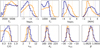 |
Fig. 11 Comparison between the posterior distributions of the high-resolution retrieval (orange; also reported in Fig. A.1) and the joint retrieval with photometric data (blue; also reported in Fig. A.2). The parameters of both retrievals agree within the 1σ confidence intervals for the bounded parameters and the 2σ intervals for the upper and lower limits (shown as dashed vertical lines; the median is omitted for clarity). The most pronounced discrepancies are found in the parameter distributions describing the low-altitude atmosphere and the chemical conditions, i.e., T2, p2, [M/H], and C/O. |
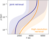 |
Fig. 12 Comparison of retrieved T-p profiles. The temperature profile inferred by the high-resolution CRIRES+ retrieval is shown in orange, the temperature profile derived from the joint retrieval with TESS and CHEOPS data is shown in blue. The solid lines correspond to the median, the shaded area to the 95 percentile intervals of the sampled temperature profiles. |
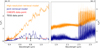 |
Fig. 13 Comparison of model spectra obtained from best-fit parameters of the retrievals. Left panel: low-resolution model spectra before integration over the TESS and CHEOPS bandpasses. The parameters derived from the high-resolution retrieval on the CRIRES+ data alone cannot constrain the planetary emission spectrum in the TESS and CHEOPS wavelength range, while the model obtained from the joint retrieval is in agreement with the photometric data points. We note that the plotted eclipse depths are corrected for their reflection component via the retrieved geometric albedo value, since the reported model spectra only consider thermal emission. Right panel: high-resolution model spectra at CRIRES+ wavelengths. Except for the different continuum level, the two models strongly resemble each other. |
6 Conclusions
We have studied the dayside emission spectrum of the UHJ WASP-178b by analyzing high-resolution spectral observations with CRIRES+ in the K band. Using the cross-correlation technique and a Bayesian retrieval framework that includes space-based photometric measurements, the following main results were obtained:
We identified the spectral signatures of the two molecular species 12CO and H2O. These are the chemical species with the most dominant emission lines in the spectral K band, and are among the most important carbon- and oxygen-bearing species. No significant signature of the chemical species 13CO, OH, and Fe I could be identified in our high-resolution spectroscopy data (Sec. 4.3);
The detections of the 12CO and H2O spectral lines in emission unambiguously prove the existence of a thermal inversion layer in WASP-178b’s atmosphere, which is in agreement with theoretical predictions (Sec. 4.3). The retrieval on the high-resolution spectroscopy data alone constrains the top and bottom of the thermal inversion layer poorly (Sect. 5.2.1). However, conducting a joint retrieval with secondary eclipse depth measurements from TESS and CHEOPS enables us to obtain tighter uncertainty intervals on the T-p profile compared to using CRIRES+ data alone (Sect. 5.2.2). The improved constraints are due to the ability of space-based measurements to capture the information of the spectral continuum level that probes the low-altitude atmospheric layers and the general lack of flux calibration in our high-resolution spectra;
The improved precision on the T-p profile obtained from the inclusion of TESS and CHEOPS data points allows a better determination of the atmospheric chemical conditions. The inferred metallicity corresponds to solar to super-solar chemical abundances, which is in line with the metallicity of the host star. The C/O ratio is consistent with the solar value. In particular, a significant improvement in the C/O ratio constraints is achieved by including space-based photometric data in our analysis (Sect. 5.2.2). We emphasize that instead of assuming constant vertical abundances that ignore the presence of thermal dissociation, we approximate the VMRs of the different chemical species by solving for chemical equilibrium in each sampling step of the retrieval (Sec. 5.1);
The emission lines of 12CO and H2O show a Doppler-shift relative to each other, indicating the presence of chemical inhomogeneities of the different species in combination with winds across the planetary surface (Sec. 4.3). In addition, we infer the presence of strong spectral line broadening that cannot be explained by planetary rotation alone. This excess broadening is most likely caused by a super-rotating atmosphere, the presence of which is generally predicted by general circulation models of UHJs (Sec. 5.2);
Finally, the inclusion of photometric data allows us to place an upper limit on the geometric albedo of WASP-178b’s dayside atmosphere, in agreement with previous photometric-only measurements (Sect. 5.2.2).
The present study on WASP-178b highlights the potential of combining ground-based high-resolution spectroscopy with spaceborne data to advance our understanding of the physical, chemical, and dynamical properties of UHJ atmospheres. Despite this potential, only a limited number of studies have explored this approach (e.g., Brogi et al. 2017; Gandhi et al. 2019; Yan et al. 2022b; Boucher et al. 2023; Smith et al. 2024). Further advances in atmospheric retrieval techniques will therefore be beneficial to fully exploit the synergies between state-of-the-art ground- and space-based facilities such as CRIRES+ and JWST.
Acknowledgements
The authors thank the referee for very useful comments and suggestions. CRIRES+ is an ESO upgrade project carried out by Thüringer Landessternwarte Tautenburg, Georg-August Universität Göttingen, and Uppsala University. The project is funded by the Federal Ministry of Education and Research (Germany) through Grants 05A11MG3, 05A14MG4, 05A17MG2 and the Knut and Alice Wallenberg Foundation. This project is based on observations collected at the European Organisation for Astronomical Research in the Southern Hemisphere under the ESO programme 111.254J.001. D.C. is supported by the LMU-Munich Fraunhofer-Schwarzschild Fellowship and by the Deutsche Forschungsgemeinschaft (DFG, German Research Foundation) under Germany’s Excellence Strategy – EXC 2094 – 390783311. F.Y. acknowledges the support by the National Natural Science Foundation of China (grant No. 42375118). F.L. acknowledges the support by the Deutsche Forschungsgemeinschaft (DFG, German Research Foundation) – Project number 314665159. S.C. and M.R acknowledge the support of the DFG priority program SPP 1992 “Exploring the Diversity of Extrasolar Planets” (CZ 222/5-1, RE 1664/16-1, and DFG PR 36 24602/41). N.P., L.B.-Ch., and A.D.R. acknowledge support by the Knut and Alice Wallenberg Foundation (grant 2018.0192). E.N. acknowledges the support by the DFG Research Unit FOR2544 “Blue Planets around Red Stars”. D.S. acknowledges financial support from the project PID2021-126365NB-C21(MCI/AEI/FEDER, UE) and from the Severo Ochoa grant CEX2021-001131-S funded by MCIN/AEI/10.13039/501100011033. This work has made use of the following Python packages: Astropy (Astropy Collaboration 2013), CMasher (van der Velden 2020), corner (Foreman-Mackey 2016), GNU Parallel (Tange 2021), Matplotlib (Hunter 2007), NumPy (Harris et al. 2020), PyAstronomy (Czesla et al. 2019), and SciPy (Virtanen et al. 2020). The authors would also like to thank Paul Mollière for his assistance in selecting the molecular line lists and calculating the high-resolution opacity files for use in petitRADTRANS.
Appendix A Posterior distributions
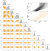 |
Fig. A.1 Results of high-resolution retrieval. Corner plot: posterior distributions and correlations between the atmospheric parameters. The dashed vertical lines in the posterior distributions denote the median and 1σ intervals for the bounded parameters. For parameters with upper or lower limits, we report the 2σ intervals. Panel a: examples of the T-p profiles sampled by the MCMC analysis, showing that the bottom of the thermal inversion is poorly constrained. Panel b: median temperature curve with 95 percentiles derived from 3000 random posterior draws. |
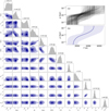 |
Fig. A.2 Same as Fig. A.1, but for joint retrieval with photometric data. The T-p profiles sampled by the MCMC analysis constrain the thermal inversion better compared to the high-resolution retrieval. |
References
- Alonso-Floriano, F. J., Sánchez-López, A., Snellen, I. A. G., et al. 2019, A&A, 621, A74 [NASA ADS] [CrossRef] [EDP Sciences] [Google Scholar]
- Arcangeli, J., Désert, J.-M., Line, M. R., et al. 2018, ApJ, 855, L30 [Google Scholar]
- Asplund, M., Grevesse, N., Sauval, A. J., & Scott, P. 2009, ARA&A, 47, 481 [NASA ADS] [CrossRef] [Google Scholar]
- Astropy Collaboration (Robitaille, T. P., et al.) 2013, A&A, 558, A33 [NASA ADS] [CrossRef] [EDP Sciences] [Google Scholar]
- Azevedo Silva, T., Demangeon, O. D. S., Santos, N. C., et al. 2022, A&A, 666, L10 [NASA ADS] [CrossRef] [EDP Sciences] [Google Scholar]
- Bazinet, L., Pelletier, S., Benneke, B., Salinas, R., & Mace, G. N. 2024, AJ, 167, 206 [NASA ADS] [CrossRef] [Google Scholar]
- Bell, T. J., & Cowan, N. B. 2018, ApJ, 857, L20 [Google Scholar]
- Bello-Arufe, A., Buchhave, L. A., Mendonça, J. M., et al. 2022a, A&A, 662, A51 [NASA ADS] [CrossRef] [EDP Sciences] [Google Scholar]
- Bello-Arufe, A., Cabot, S. H. C., Mendonça, J. M., Buchhave, L. A., & Rathcke, A. D. 2022b, AJ, 163, 96 [NASA ADS] [CrossRef] [Google Scholar]
- Beltz, H., Rauscher, E., Brogi, M., & Kempton, E. M. R. 2021, AJ, 161, 1 [Google Scholar]
- Ben-Yami, M., Madhusudhan, N., Cabot, S. H. C., et al. 2020, ApJ, 897, L5 [CrossRef] [Google Scholar]
- Birkby, J. L. 2018, in Handbook of Exoplanets, eds. H. J. Deeg, & J. A. Belmonte (Springer), 16 [Google Scholar]
- Birkby, J. L., de Kok, R. J., Brogi, M., et al. 2013, MNRAS, 436, L35 [Google Scholar]
- Borsa, F., Allart, R., Casasayas-Barris, N., et al. 2021a, A&A, 645, A24 [NASA ADS] [CrossRef] [EDP Sciences] [Google Scholar]
- Borsa, F., Fossati, L., Koskinen, T., Young, M. E., & Shulyak, D. 2021b, Nat. Astron., 6, 226 [NASA ADS] [CrossRef] [Google Scholar]
- Borsa, F., Lanza, A. F., Raspantini, I., et al. 2021c, A&A, 653, A104 [NASA ADS] [CrossRef] [EDP Sciences] [Google Scholar]
- Borsa, F., Giacobbe, P., Bonomo, A. S., et al. 2022, A&A, 663, A141 [NASA ADS] [CrossRef] [EDP Sciences] [Google Scholar]
- Borsato, N. W., Hoeijmakers, H. J., Prinoth, B., et al. 2023, A&A, 673, A158 [NASA ADS] [CrossRef] [EDP Sciences] [Google Scholar]
- Borsato, N. W., Hoeijmakers, H. J., Cont, D., et al. 2024, A&A, 683, A98 [NASA ADS] [CrossRef] [EDP Sciences] [Google Scholar]
- Boucher, A., Lafreniére, D., Pelletier, S., et al. 2023, MNRAS, 522, 5062 [NASA ADS] [CrossRef] [Google Scholar]
- Brogi, M., & Line, M. R. 2019, AJ, 157, 114 [Google Scholar]
- Brogi, M., Snellen, I. A. G., de Kok, R. J., et al. 2012, Nature, 486, 502 [Google Scholar]
- Brogi, M., Line, M., Bean, J., Désert, J. M., & Schwarz, H. 2017, ApJ, 839, L2 [Google Scholar]
- Brogi, M., Emeka-Okafor, V., Line, M. R., et al. 2023, AJ, 165, 91 [NASA ADS] [CrossRef] [Google Scholar]
- Brooke, J. S. A., Bernath, P. F., Western, C. M., et al. 2016, J. Quant. Spec. Radiat. Transf., 168, 142 [NASA ADS] [CrossRef] [Google Scholar]
- Cabot, S. H. C., Madhusudhan, N., Welbanks, L., Piette, A., & Gandhi, S. 2020, MNRAS, 494, 363 [Google Scholar]
- Cabot, S. H. C., Bello-Arufe, A., Mendonça, J. M., et al. 2021, AJ, 162, 218 [NASA ADS] [CrossRef] [Google Scholar]
- Casasayas-Barris, N., Pallé, E., Yan, F., et al. 2018, A&A, 616, A151 [NASA ADS] [CrossRef] [EDP Sciences] [Google Scholar]
- Casasayas-Barris, N., Pallé, E., Yan, F., et al. 2019, A&A, 628, A9 [NASA ADS] [CrossRef] [EDP Sciences] [Google Scholar]
- Casasayas-Barris, N., Orell-Miquel, J., Stangret, M., et al. 2021, A&A, 654, A163 [NASA ADS] [CrossRef] [EDP Sciences] [Google Scholar]
- Cont, D., Yan, F., Reiners, A., et al. 2021, A&A, 651, A33 [NASA ADS] [CrossRef] [EDP Sciences] [Google Scholar]
- Cont, D., Yan, F., Reiners, A., et al. 2022a, A&A, 668, A53 [NASA ADS] [CrossRef] [EDP Sciences] [Google Scholar]
- Cont, D., Yan, F., Reiners, A., et al. 2022b, A&A, 657, A2 [Google Scholar]
- Czesla, S., Schröter, S., Schneider, C. P., et al. 2019, PyA: Python astronomy-related packages, Astrophysics Source Code Library [record ascl:1986.818] [Google Scholar]
- Czesla, S., Schneider, P. C., & Hatzes, A. 2023, A&A, 677, L12 [NASA ADS] [CrossRef] [EDP Sciences] [Google Scholar]
- Czesla, S., Lampón, M., Cont, D., et al. 2024, A&A, 683, A67 [NASA ADS] [CrossRef] [EDP Sciences] [Google Scholar]
- Damasceno, Y. C., Seidel, J. V., Prinoth, B., et al. 2024, A&A, in press, https://doi.org/10.1051/0004-6361/202450119 [Google Scholar]
- Deibert, E. K., de Mooij, E. J. W., Jayawardhana, R., et al. 2021, ApJ, 919, L15 [NASA ADS] [CrossRef] [Google Scholar]
- Deibert, E. K., de Mooij, E. J. W., Jayawardhana, R., et al. 2023, AJ, 166, 141 [NASA ADS] [CrossRef] [Google Scholar]
- Díaz, C. G., González, J. F., Levato, H., & Grosso, M. 2011, A&A, 531, A143 [NASA ADS] [CrossRef] [EDP Sciences] [Google Scholar]
- Dorn, R. J., Bristow, P., Smoker, J. V., et al. 2023, A&A, 671, A24 [NASA ADS] [CrossRef] [EDP Sciences] [Google Scholar]
- Ehrenreich, D., Lovis, C., Allart, R., et al. 2020, Nature, 580, 597 [Google Scholar]
- Finnerty, L., Schofield, T., Sappey, B., et al. 2023, AJ, 166, 31 [NASA ADS] [CrossRef] [Google Scholar]
- Foreman-Mackey, D. 2016, J. Open Source Softw., 1, 24 [Google Scholar]
- Foreman-Mackey, D., Hogg, D. W., Lang, D., & Goodman, J. 2013, PASP, 125, 306 [Google Scholar]
- Fortney, J. J., Lodders, K., Marley, M. S., & Freedman, R. S. 2008, ApJ, 678, 1419 [CrossRef] [Google Scholar]
- Fossati, L., Biassoni, F., Cappello, G. M., et al. 2023, A&A, 676, A99 [NASA ADS] [CrossRef] [EDP Sciences] [Google Scholar]
- Gandhi, S., & Madhusudhan, N. 2019, MNRAS, 485, 5817 [Google Scholar]
- Gandhi, S., Madhusudhan, N., Hawker, G., & Piette, A. 2019, AJ, 158, 228 [NASA ADS] [CrossRef] [Google Scholar]
- Gandhi, S., Brogi, M., Yurchenko, S. N., et al. 2020, MNRAS, 495, 224 [NASA ADS] [CrossRef] [Google Scholar]
- Gandhi, S., Kesseli, A., Snellen, I., et al. 2022, MNRAS, 515, 749 [NASA ADS] [CrossRef] [Google Scholar]
- Gandhi, S., Kesseli, A., Zhang, Y., et al. 2023, AJ, 165, 242 [NASA ADS] [CrossRef] [Google Scholar]
- Gandhi, S., Landman, R., Snellen, I., et al. 2024, MNRAS, 530, 2885 [NASA ADS] [CrossRef] [Google Scholar]
- Gibson, N. P., Merritt, S., Nugroho, S. K., et al. 2020, MNRAS, 493, 2215 [Google Scholar]
- Gibson, N. P., Nugroho, S. K., Lothringer, J., Maguire, C., & Sing, D. K. 2022, MNRAS, 512, 4618 [NASA ADS] [CrossRef] [Google Scholar]
- Guo, B., Yan, F., Nortmann, L., et al. 2024, A&A, 687 A103 [NASA ADS] [CrossRef] [EDP Sciences] [Google Scholar]
- Harris, C. R., Millman, K. J., van der Walt, S. J., et al. 2020, Nature, 585, 357 [NASA ADS] [CrossRef] [Google Scholar]
- Hellier, C., Anderson, D. R., Barkaoui, K., et al. 2019, MNRAS, 490, 1479 [NASA ADS] [CrossRef] [Google Scholar]
- Helling, C., Gourbin, P., Woitke, P., & Parmentier, V. 2019, A&A, 626, A133 [NASA ADS] [CrossRef] [EDP Sciences] [Google Scholar]
- Heng, K., Menou, K., & Phillipps, P. J. 2011, MNRAS, 413, 2380 [NASA ADS] [CrossRef] [Google Scholar]
- Herman, M. K., de Mooij, E. J. W., Nugroho, S. K., Gibson, N. P., & Jayawardhana, R. 2022, AJ, 163, 248 [NASA ADS] [CrossRef] [Google Scholar]
- Hoeijmakers, H. J., Ehrenreich, D., Heng, K., et al. 2018, Nature, 560, 453 [CrossRef] [Google Scholar]
- Hoeijmakers, H. J., Ehrenreich, D., Kitzmann, D., et al. 2019, A&A, 627, A165 [NASA ADS] [CrossRef] [EDP Sciences] [Google Scholar]
- Hoeijmakers, H. J., Cabot, S. H. C., Zhao, L., et al. 2020a, A&A, 641, A120 [NASA ADS] [CrossRef] [EDP Sciences] [Google Scholar]
- Hoeijmakers, H. J., Seidel, J. V., Pino, L., et al. 2020b, A&A, 641, A123 [NASA ADS] [CrossRef] [EDP Sciences] [Google Scholar]
- Hoeijmakers, H. J., Kitzmann, D., Morris, B. M., et al. 2024, A&A, 685, A139 [NASA ADS] [CrossRef] [EDP Sciences] [Google Scholar]
- Holmberg, M., & Madhusudhan, N. 2022, AJ, 164, 79 [NASA ADS] [CrossRef] [Google Scholar]
- Hood, T., Debras, F., Moutou, C., et al. 2024, A&A, 687, A119 [NASA ADS] [CrossRef] [EDP Sciences] [Google Scholar]
- Hubeny, I., Burrows, A., & Sudarsky, D. 2003, ApJ, 594, 1011 [Google Scholar]
- Hunter, J. D. 2007, Comput. Sci. Eng., 9, 90 [NASA ADS] [CrossRef] [Google Scholar]
- Hut, P. 1981, A&A, 99, 126 [NASA ADS] [Google Scholar]
- Jansen, T., & Kipping, D. 2020, MNRAS, 494, 4077 [Google Scholar]
- Jensen, A. G., Cauley, P. W., Redfield, S., Cochran, W. D., & Endl, M. 2018, AJ, 156, 154 [Google Scholar]
- Jiang, Z., Wang, W., Zhao, G., et al. 2023, AJ, 165, 230 [NASA ADS] [CrossRef] [Google Scholar]
- Johnson, M. C., Wang, J., Asnodkar, A. P., et al. 2023, AJ, 165, 157 [NASA ADS] [CrossRef] [Google Scholar]
- Kasper, D., Bean, J. L., Line, M. R., et al. 2021, ApJ, 921, L18 [CrossRef] [Google Scholar]
- Kasper, D., Bean, J. L., Line, M. R., et al. 2023, AJ, 165, 7 [NASA ADS] [CrossRef] [Google Scholar]
- Kawauchi, K., Narita, N., Sato, B., & Kawashima, Y. 2022, PASJ, 74, 225 [CrossRef] [Google Scholar]
- Kesseli, A. Y., & Snellen, I. A. G. 2021, ApJ, 908, L17 [Google Scholar]
- Kesseli, A. Y., Snellen, I. A. G., Casasayas-Barris, N., Mollière, P., & Sánchez-López, A. 2022, AJ, 163, 107 [NASA ADS] [CrossRef] [Google Scholar]
- Kitzmann, D., Heng, K., Rimmer, P. B., et al. 2018, ApJ, 863, 183 [Google Scholar]
- Kitzmann, D., Heng, K., Oreshenko, M., et al. 2020, ApJ, 890, 174 [Google Scholar]
- Komacek, T. D., & Tan, X. 2018, RNAAS, 2, 36 [NASA ADS] [Google Scholar]
- Kreidberg, L., Line, M. R., Parmentier, V., et al. 2018, AJ, 156, 17 [NASA ADS] [CrossRef] [Google Scholar]
- Kurucz, R. L. 2018, in ASP Conf. Ser., 515, Workshop on Astrophysical Opacities, 47 [NASA ADS] [Google Scholar]
- Landman, R., Sánchez-López, A., Mollière, P., et al. 2021, A&A, 656, A119 [NASA ADS] [CrossRef] [EDP Sciences] [Google Scholar]
- Landman, R., Stolker, T., Snellen, I., et al. 2024, A&A, 682, A48 [NASA ADS] [CrossRef] [EDP Sciences] [Google Scholar]
- Langeveld, A. B., Madhusudhan, N., & Cabot, S. H. C. 2022, MNRAS, 514, 5192 [NASA ADS] [CrossRef] [Google Scholar]
- Lavail, A. 2024, https://doi.org/10.5281/zenodo.11637332 [Google Scholar]
- Lesjak, F., Nortmann, L., Yan, F., et al. 2023, A&A, 678, A23 [NASA ADS] [CrossRef] [EDP Sciences] [Google Scholar]
- Li, G., Gordon, I. E., Rothman, L. S., et al. 2015, ApJS, 216, 15 [NASA ADS] [CrossRef] [Google Scholar]
- Line, M. R., Zhang, X., Vasisht, G., et al. 2012, ApJ, 749, 93 [Google Scholar]
- Line, M. R., Brogi, M., Bean, J. L., et al. 2021, Nature, 598, 580 [NASA ADS] [CrossRef] [Google Scholar]
- Lothringer, J. D., & Barman, T. 2019, ApJ, 876, 69 [Google Scholar]
- Lothringer, J. D., Barman, T., & Koskinen, T. 2018, ApJ, 866, 27 [NASA ADS] [CrossRef] [Google Scholar]
- Lothringer, J. D., Sing, D. K., Rustamkulov, Z., et al. 2022, Nature, 604, 49 [NASA ADS] [CrossRef] [Google Scholar]
- Lowson, N., Zhou, G., Wright, D. J., et al. 2023, AJ, 165, 101 [NASA ADS] [CrossRef] [Google Scholar]
- MacDonald, R. J., & Batalha, N. E. 2023, RNAAS, 7, 54 [NASA ADS] [Google Scholar]
- Madhusudhan, N. 2012, ApJ, 758, 36 [NASA ADS] [CrossRef] [Google Scholar]
- Madhusudhan, N., & Seager, S. 2009, ApJ, 707, 24 [NASA ADS] [CrossRef] [Google Scholar]
- Maguire, C., Gibson, N. P., Nugroho, S. K., et al. 2023, MNRAS, 519, 1030 [Google Scholar]
- Maguire, C., Gibson, N. P., Nugroho, S. K., et al. 2024, A&A, 687, A49 [NASA ADS] [CrossRef] [EDP Sciences] [Google Scholar]
- Mallonn, M., Köhler, J., Alexoudi, X., et al. 2019, A&A, 624, A62 [NASA ADS] [CrossRef] [EDP Sciences] [Google Scholar]
- Merritt, S. R., Gibson, N. P., Nugroho, S. K., et al. 2020, A&A, 636, A117 [NASA ADS] [CrossRef] [EDP Sciences] [Google Scholar]
- Merritt, S. R., Gibson, N. P., Nugroho, S. K., et al. 2021, MNRAS, 506, 3853 [NASA ADS] [CrossRef] [Google Scholar]
- Mollière, P., Wardenier, J. P., van Boekel, R., et al. 2019, A&A, 627, A67 [Google Scholar]
- Mordasini, C., van Boekel, R., Mollière, P., Henning, T., & Benneke, B. 2016, ApJ, 832, 41 [Google Scholar]
- Nortmann, L., Lesjak, F., Yan, F., et al. 2024, A&A, submitted [arXiv:2404.12363] [Google Scholar]
- Nugroho, S. K., Kawahara, H., Masuda, K., et al. 2017, AJ, 154, 221 [Google Scholar]
- Nugroho, S. K., Gibson, N. P., de Mooij, E. J. W., et al. 2020a, ApJ, 898, L31 [NASA ADS] [CrossRef] [Google Scholar]
- Nugroho, S. K., Gibson, N. P., de Mooij, E. J. W., et al. 2020b, MNRAS, 496, 504 [NASA ADS] [CrossRef] [Google Scholar]
- Nugroho, S. K., Kawahara, H., Gibson, N. P., et al. 2021, ApJ, 910, L9 [CrossRef] [Google Scholar]
- Öberg, K. I., Murray-Clay, R., & Bergin, E. A. 2011, ApJ, 743, L16 [Google Scholar]
- Pagano, I., Scandariato, G., Singh, V., et al. 2024, A&A, 682, A102 [NASA ADS] [CrossRef] [EDP Sciences] [Google Scholar]
- Pai Asnodkar, A., Wang, J., Eastman, J. D., et al. 2022, AJ, 163, 155 [NASA ADS] [CrossRef] [Google Scholar]
- Parmentier, V., Line, M. R., Bean, J. L., et al. 2018, A&A, 617, A110 [NASA ADS] [CrossRef] [EDP Sciences] [Google Scholar]
- Pelletier, S., Benneke, B., Darveau-Bernier, A., et al. 2021, AJ, 162, 73 [NASA ADS] [CrossRef] [Google Scholar]
- Pelletier, S., Benneke, B., Ali-Dib, M., et al. 2023, Nature, 619, 491 [NASA ADS] [CrossRef] [Google Scholar]
- Petz, S., Johnson, M. C., Asnodkar, A. P., et al. 2024, MNRAS, 527, 7079 [Google Scholar]
- Piette, A. A. A., Madhusudhan, N., McKemmish, L. K., et al. 2020, MNRAS, 496, 3870 [Google Scholar]
- Pino, L., Désert, J.-M., Brogi, M., et al. 2020, ApJ, 894, L27 [Google Scholar]
- Pino, L., Brogi, M., Désert, J. M., et al. 2022, A&A, 668, A176 [NASA ADS] [CrossRef] [EDP Sciences] [Google Scholar]
- Polyansky, O. L., Kyuberis, A. A., Zobov, N. F., et al. 2018, MNRAS, 480, 2597 [NASA ADS] [CrossRef] [Google Scholar]
- Prinoth, B., Hoeijmakers, H. J., Kitzmann, D., et al. 2022, Nat. Astron., 6, 449 [NASA ADS] [CrossRef] [Google Scholar]
- Prinoth, B., Hoeijmakers, H. J., Pelletier, S., et al. 2023, A&A, 678, A182 [NASA ADS] [CrossRef] [EDP Sciences] [Google Scholar]
- Prinoth, B., Hoeijmakers, H. J., Morris, B. M., et al. 2024, A&A, 685, A60 [NASA ADS] [CrossRef] [EDP Sciences] [Google Scholar]
- Ramkumar, S., Gibson, N. P., Nugroho, S. K., Maguire, C., & Fortune, M. 2023, MNRAS, 525, 2985 [CrossRef] [Google Scholar]
- Rengel, M., & Adamczewski, J. 2023, Front. Astron. Space Sci., 10, 1176740 [NASA ADS] [CrossRef] [Google Scholar]
- Ridden-Harper, A., de Mooij, E., Jayawardhana, R., et al. 2023, AJ, 165, 211 [NASA ADS] [CrossRef] [Google Scholar]
- Rodríguez Martínez, R., Gaudi, B. S., Rodriguez, J. E., et al. 2020, AJ, 160, 111 [CrossRef] [Google Scholar]
- Sánchez-López, A., Alonso-Floriano, F. J., López-Puertas, M., et al. 2019, A&A, 630, A53 [NASA ADS] [CrossRef] [EDP Sciences] [Google Scholar]
- Sánchez-López, A., Landman, R., Mollière, P., et al. 2022a, A&A, 661, A78 [NASA ADS] [CrossRef] [EDP Sciences] [Google Scholar]
- Sánchez-López, A., Lin, L., Snellen, I. A. G., et al. 2022b, A&A, 666, L1 [NASA ADS] [CrossRef] [EDP Sciences] [Google Scholar]
- Scandariato, G., Borsa, F., Bonomo, A. S., et al. 2023, A&A, 674, A58 [NASA ADS] [CrossRef] [EDP Sciences] [Google Scholar]
- Sedaghati, E., MacDonald, R. J., Casasayas-Barris, N., et al. 2021, MNRAS, 505, 435 [NASA ADS] [CrossRef] [Google Scholar]
- Seidel, J. V., Ehrenreich, D., Wyttenbach, A., et al. 2019, A&A, 623, A166 [NASA ADS] [CrossRef] [EDP Sciences] [Google Scholar]
- Seidel, J. V., Ehrenreich, D., Allart, R., et al. 2021, A&A, 653, A73 [NASA ADS] [CrossRef] [EDP Sciences] [Google Scholar]
- Seidel, J. V., Borsa, F., Pino, L., et al. 2023, A&A, 673, A125 [NASA ADS] [CrossRef] [EDP Sciences] [Google Scholar]
- Showman, A. P., Fortney, J. J., Lian, Y., et al. 2009, ApJ, 699, 564 [NASA ADS] [CrossRef] [Google Scholar]
- Showman, A. P., Fortney, J. J., Lewis, N. K., & Shabram, M. 2013, ApJ, 762, 24 [Google Scholar]
- Shulyak, D., Rengel, M., Reiners, A., Seemann, U., & Yan, F. 2019, A&A, 629, A109 [NASA ADS] [CrossRef] [EDP Sciences] [Google Scholar]
- Shulyak, D., Lara, L. M., Rengel, M., & Nèmec, N. E. 2020, A&A, 639, A48 [NASA ADS] [CrossRef] [EDP Sciences] [Google Scholar]
- Smette, A., Sana, H., Noll, S., et al. 2015, A&A, 576, A77 [NASA ADS] [CrossRef] [EDP Sciences] [Google Scholar]
- Smith, P. C. B., Line, M. R., Bean, J. L., et al. 2024, AJ, 167, 110 [NASA ADS] [CrossRef] [Google Scholar]
- Snellen, I. A. G., de Kok, R. J., de Mooij, E. J. W., & Albrecht, S. 2010, Nature, 465, 1049 [Google Scholar]
- Stangret, M., Casasayas-Barris, N., Pallé, E., et al. 2020, A&A, 638, A26 [NASA ADS] [CrossRef] [EDP Sciences] [Google Scholar]
- Stangret, M., Casasayas-Barris, N., Pallé, E., et al. 2022, A&A, 662, A101 [NASA ADS] [CrossRef] [EDP Sciences] [Google Scholar]
- Stock, J. W., Kitzmann, D., Patzer, A. B. C., & Sedlmayr, E. 2018, MNRAS, 479, 865 [NASA ADS] [Google Scholar]
- Tabernero, H. M., Zapatero Osorio, M. R., Allart, R., et al. 2021, A&A, 646, A158 [NASA ADS] [CrossRef] [EDP Sciences] [Google Scholar]
- Tamuz, O., Mazeh, T., & Zucker, S. 2005, MNRAS, 356, 1466 [Google Scholar]
- Tan, X., & Komacek, T. D. 2019, ApJ, 886, 26 [Google Scholar]
- Tange, O. 2021, https://doi.org/10.5281/zenodo.5233953 [Google Scholar]
- van der Velden, E. 2020, J. Open Source Softw., 5, 2004 [Google Scholar]
- van Sluijs, L., Birkby, J. L., Lothringer, J., et al. 2023, MNRAS, 522, 2145 [NASA ADS] [CrossRef] [Google Scholar]
- Virtanen, P., Gommers, R., Oliphant, T. E., et al. 2020, Nature Methods, 17, 261 [CrossRef] [Google Scholar]
- Weiner Mansfield, M., Line, M. R., Wardenier, J. P., et al. 2024, AJ, accepted [arXiv:2405.09769] [Google Scholar]
- Wong, I., Benneke, B., Shporer, A., et al. 2020, AJ, 159, 104 [Google Scholar]
- Wong, I., Kitzmann, D., Shporer, A., et al. 2021, AJ, 162, 127 [NASA ADS] [CrossRef] [Google Scholar]
- Wright, S. O. M., Nugroho, S. K., Brogi, M., et al. 2023, AJ, 166, 41 [NASA ADS] [CrossRef] [Google Scholar]
- Wyttenbach, A., Mollière, P., Ehrenreich, D., et al. 2020, A&A, 638, A87 [EDP Sciences] [Google Scholar]
- Yan, F., & Henning, T. 2018, Nat. Astron., 2, 714 [Google Scholar]
- Yan, F., Casasayas-Barris, N., Molaverdikhani, K., et al. 2019, A&A, 632, A69 [NASA ADS] [CrossRef] [EDP Sciences] [Google Scholar]
- Yan, F., Pallé, E., Reiners, A., et al. 2020, A&A, 640, L5 [NASA ADS] [CrossRef] [EDP Sciences] [Google Scholar]
- Yan, F., Wyttenbach, A., Casasayas-Barris, N., et al. 2021, A&A, 645, A22 [EDP Sciences] [Google Scholar]
- Yan, F., Pallé, E., Reiners, A., et al. 2022a, A&A, 661, L6 [NASA ADS] [CrossRef] [EDP Sciences] [Google Scholar]
- Yan, F., Reiners, A., Pallé, E., et al. 2022b, A&A, 659, A7 [NASA ADS] [CrossRef] [EDP Sciences] [Google Scholar]
- Yan, F., Nortmann, L., Reiners, A., et al. 2023, A&A, 672, A107 [NASA ADS] [CrossRef] [EDP Sciences] [Google Scholar]
- Yang, Y., Chen, G., Wang, S., & Yan, F. 2024, AJ, 167, 36 [CrossRef] [Google Scholar]
- Young, M. E., Spring, E. F., & Birkby, J. L. 2024, MNRAS, 530, 4356 [NASA ADS] [CrossRef] [Google Scholar]
- Zhang, Y., Snellen, I. A. G., Bohn, A. J., et al. 2021, Nature, 595, 370 [NASA ADS] [CrossRef] [Google Scholar]
- Zhang, Y., Snellen, I. A. G., Wyttenbach, A., et al. 2022, A&A, 666, A47 [NASA ADS] [CrossRef] [EDP Sciences] [Google Scholar]
Retrieved from the Exoplanet Atmospheres Database at https://research.iac.es/proyecto/exoatmospheres/
The extracted data, together with the refined wavelength solution, are available at https://zenodo.org/records/11637332 (Lavail 2024).
All Tables
Summary of chemical species detected via high-resolution spectroscopy in UHJ atmospheres, retrieved from the Exoplanet Atmospheres Database as of May 2024.
All Figures
|
Fig. 1 Evolution of the airmass (top panel) and the mean S/N per detector pixel (bottom panel). Data points corresponding to the A and B nodding positions are shown in orange and blue, respectively. |
| In the text | |
|
Fig. 2 RV drift during the acquisition of the spectral time series. Each data point corresponds to an individual exposure frame and wavelength segment. Data points corresponding to the A and B nodding positions are shown in orange and blue, respectively. |
| In the text | |
|
Fig. 3 Overview of data reduction procedures for a representative CRIRES+ wavelength range. Panel a: raw spectral matrix after extraction of the one-dimensional spectra. Panel b: spectral matrix after normalization, outlier correction, and masking of the strongest telluric features. Panel c: residual spectral matrix after removal of telluric and stellar lines via two consecutive SYSREM iterations. |
| In the text | |
|
Fig. 4 Volume mixing ratios (VMRs; left panel) and T-p profile (right panel) used to generate the model spectra for cross-correlation. The VMRs were calculated assuming equilibrium chemistry. The elemental abundances and the T-p profile used correspond to the best-fit results of the retrieval framework in Sec. 5. |
| In the text | |
|
Fig. 5 Spectral models, CCF maps, and S/N maps of 12CO, H2O, and both species together. The left panels show the continuum normalized model spectra. Wavelengths covered by the CRIRES+ K2166 setting used in this work are indicated by the gray shaded area. The middle panels illustrate the CCF maps. The spectral signal from WASP-178b’s atmosphere can be identified as a diagonal trail. The expected RV evolution as a function of orbital phase is indicated by the yellow dashed lines. The right panels show the S/N maps. The expected position of the planetary signal is indicated by the yellow dashed lines. We show the CCF maps and S/N maps corresponding to two consecutive runs of SYSREM, which is the number of iterations used in the retrieval in Sec. 5. |
| In the text | |
|
Fig. 6 Same as Fig. 5, but for 13CO, OH, and Fe I. These species result in non-detections due to the weakness and low number of spectral lines over the investigated wavelength range. The CCF maps and S/N maps are the result of two consecutive SYSREM iterations. |
| In the text | |
|
Fig. 7 S/N values as a function of SYSREM iterations. We show the detection strengths obtained from cross-correlation with model spectra including the emission lines of 12CO, H2O, and both species together, respectively. The iteration with the most significant S/N peak is indicated by the star symbol. In our retrieval framework in Sec. 5, we used the iteration number that yields the most prominent S/N detection peak of the species-combined signal, i.e., two consecutive SYSREM iterations. |
| In the text | |
|
Fig. 8 One-sigma regions of 12CO and H2O detections. The position of the 12CO signal is inconsistent, that of the H2O signal is consistent with the expected Kp and υsys values, whose location is indicated by the red symbols (“+”: Hellier et al. 2019; “×”: Rodríguez Martínez et al. 2020). |
| In the text | |
|
Fig. 9 S/N maps of injection-recovery test. The yellow dashed lines indicate the coordinates of the injected signal. The injected signatures of 13CO, OH, and Fe I could not be identified, indicating that even if present in the planetary atmosphere, these species are undetectable. |
| In the text | |
|
Fig. 10 Comparison between model spectra computed with 25 (top panel) and 81 (middle panel) atmospheric layers. The model spectra include the opacities of the detected chemical species 12CO and H2O, as well as those of H−. The difference between the models is insignificant (bottom panel), implying that the lower number of atmospheric layers does not significantly affect our retrieval results. |
| In the text | |
|
Fig. 11 Comparison between the posterior distributions of the high-resolution retrieval (orange; also reported in Fig. A.1) and the joint retrieval with photometric data (blue; also reported in Fig. A.2). The parameters of both retrievals agree within the 1σ confidence intervals for the bounded parameters and the 2σ intervals for the upper and lower limits (shown as dashed vertical lines; the median is omitted for clarity). The most pronounced discrepancies are found in the parameter distributions describing the low-altitude atmosphere and the chemical conditions, i.e., T2, p2, [M/H], and C/O. |
| In the text | |
|
Fig. 12 Comparison of retrieved T-p profiles. The temperature profile inferred by the high-resolution CRIRES+ retrieval is shown in orange, the temperature profile derived from the joint retrieval with TESS and CHEOPS data is shown in blue. The solid lines correspond to the median, the shaded area to the 95 percentile intervals of the sampled temperature profiles. |
| In the text | |
|
Fig. 13 Comparison of model spectra obtained from best-fit parameters of the retrievals. Left panel: low-resolution model spectra before integration over the TESS and CHEOPS bandpasses. The parameters derived from the high-resolution retrieval on the CRIRES+ data alone cannot constrain the planetary emission spectrum in the TESS and CHEOPS wavelength range, while the model obtained from the joint retrieval is in agreement with the photometric data points. We note that the plotted eclipse depths are corrected for their reflection component via the retrieved geometric albedo value, since the reported model spectra only consider thermal emission. Right panel: high-resolution model spectra at CRIRES+ wavelengths. Except for the different continuum level, the two models strongly resemble each other. |
| In the text | |
|
Fig. A.1 Results of high-resolution retrieval. Corner plot: posterior distributions and correlations between the atmospheric parameters. The dashed vertical lines in the posterior distributions denote the median and 1σ intervals for the bounded parameters. For parameters with upper or lower limits, we report the 2σ intervals. Panel a: examples of the T-p profiles sampled by the MCMC analysis, showing that the bottom of the thermal inversion is poorly constrained. Panel b: median temperature curve with 95 percentiles derived from 3000 random posterior draws. |
| In the text | |
|
Fig. A.2 Same as Fig. A.1, but for joint retrieval with photometric data. The T-p profiles sampled by the MCMC analysis constrain the thermal inversion better compared to the high-resolution retrieval. |
| In the text | |
Current usage metrics show cumulative count of Article Views (full-text article views including HTML views, PDF and ePub downloads, according to the available data) and Abstracts Views on Vision4Press platform.
Data correspond to usage on the plateform after 2015. The current usage metrics is available 48-96 hours after online publication and is updated daily on week days.
Initial download of the metrics may take a while.