| Issue |
A&A
Volume 695, March 2025
|
|
|---|---|---|
| Article Number | A110 | |
| Number of page(s) | 29 | |
| Section | Planets, planetary systems, and small bodies | |
| DOI | https://doi.org/10.1051/0004-6361/202453520 | |
| Published online | 13 March 2025 | |
New perspectives on MASCARA-1b: A combined analysis of pre- and post-eclipse emission data using CRIRES+
1
School of Physics, Trinity College Dublin, University of Dublin,
Dublin-2, Ireland
2
Astrobiology Center, NINS,
2-21-1 Osawa,
Mitaka, Tokyo
181-8588, Japan
3
National Astronomical Observatory of Japan,
2-21-1 Osawa,
Mitaka, Tokyo
181-8588, Japan
★ Corresponding author; This email address is being protected from spambots. You need JavaScript enabled to view it.
Received:
19
December
2024
Accepted:
14
February
2025
Abstract
Aims. We present high-resolution emission spectroscopy observations of the ultra-hot Jupiter MASCARA-1b with CRIRES+ in the K-band, covering the post-eclipse phases of the planet’s orbit. These observations complement previously published pre-eclipse data.
Methods. The stellar and telluric features were removed from the data using the SYSREM algorithm, and the planetary signal was analysed with the cross-correlation technique. After confirming the presence of chemical species in our atmospheric model, we combined the pre- and post-eclipse datasets for a joint analysis. By employing a Bayesian retrieval framework with various parametrisations, this joint retrieval enabled us to constrain the spatially varying temperature-pressure (T–P) profile and the atmospheric carbon-to-oxygen (C/O) ratio.
Results. We detected strong emission signatures of CO and H2O in the post-eclipse and the combined datasets. A well-mixed retrieval model results in a super-solar C/O, whereas allowing for vertically varying chemistry by incorporating a chemical model results in C/O values consistent with solar within ≈1.1σ. The retrieved parameters are not only consistent across the datasets but also across different chemical regimes. We did not identify any significant velocity shifts between the detected species or across the datasets that could otherwise serve as proxies for possible atmospheric dynamics. We also explored potential phase dependence through the model scaling factor and found no substantial changes in the atmospheric properties throughout the observed phases.
Conclusions. Due to strong degeneracies between the temperature gradient and chemical abundances, our retrieved temperatures are broadly consistent with either a full redistribution of heat or strong day-night contrasts. While this complicates direct comparisons with recent Spitzer phase curve analyses suggesting inefficient recirculation, we find no clear evidence of spatial variation in the chemical or temperature structure of MASCARA-1b from pre- to post-eclipse, nor temporal variation over a period of ≈2 years.
Key words: methods: data analysis / methods: observational / techniques: spectroscopic / planets and satellites: atmospheres / planets and satellites: individual: MASCARA-1b
© The Authors 2025
 Open Access article, published by EDP Sciences, under the terms of the Creative Commons Attribution License (https://creativecommons.org/licenses/by/4.0), which permits unrestricted use, distribution, and reproduction in any medium, provided the original work is properly cited.
This article is published in open access under the Subscribe to Open model. This email address is being protected from spambots. You need JavaScript enabled to view it. to support open access publication.
1 Introduction
One of the most profound discoveries in the last decades in astronomy is that exoplanets are extremely common in the Universe. This discovery has not only introduced us to a range of strange and exciting worlds fundamentally different from the planets in our Solar System but has also allowed us to gain a deeper insight into their formation and evolution. Transit observations of exoplanets are crucial for comparative studies, and when combined with radial velocity data, these measurements allow the inference of the planet’s mass, radius, and composition. However, little is known about the processes that determine the atmospheric structure of these planets, which highlights the need for spectroscopic observations using space-based and ground-based instruments.
In particular, high-resolution cross-correlation spectroscopy (HRCCS) has emerged as a powerful technique for characterising exoplanetary atmospheres. With significant advancements in ground-based high-spectral resolution platforms (e.g. CRIRES+, ESPRESSO, IGRINS, IRD; Dorn et al. 2014, 2023; Pepe et al. 2021; Park et al. 2014; Mace et al. 2018; Tamura et al. 2012; Kotani et al. 2018), HRCCS has become instrumental in constraining basic atmospheric properties. First demonstrated by the detection of CO in the hot Jupiter HD 209458b (Snellen et al. 2010) using the CRyogenic high-resolution InfraRed Echelle Spectrograph (CRIRES; Kaeufl et al. 2004), HRCCS observations leverage the planetary Doppler shift of the dense forest of individually resolved spectral lines to detect both atomic and molecular species robustly. Since then, it has been used to detect several chemical species in the atmospheres of exoplanets, particularly those of close-in giant planets, such as hot and ultra-hot Jupiters (UHJs). Due to their proximity to their host stars, these tidally locked gas giants are a fascinating population without similar counterparts in our Solar System. Their high equilibrium temperatures (Teq ≳ 2200 K) not only create conditions where major C- and O-bearing species (such as CO, OH and atomic O) are expected to exist in gaseous form but they also have a significant impact on their atmospheric structure and composition, such as the occurrence of inversion layers due to the presence of molecular compounds like TiO and VO (Prinoth et al. 2022; Pelletier et al. 2023; Maguire et al. 2024) high up in the atmospheres as well as due to absorption by atomic metals and metal hydrides (Lothringer et al. 2018; Gandhi & Madhusudhan 2019; Flagg et al. 2023). This makes UHJs ideal targets for atmospheric characterisation wherein they serve as a treasure trove for numerous chemical species (e.g. Fe I, Fe II, Ca I, Ca II, OH, CO, H2O, etc.) that have been detected using high-resolution transmission and emission spectroscopy (e.g. Hoeijmakers et al. 2019; Gibson et al. 2020; Pino et al. 2020; Maguire et al. 2023; Nugroho et al. 2021; Brogi et al. 2023; Ramkumar et al. 2023).
The HRCCS technique is not limited to transmission spectroscopy; it is also powerful when applied to emission spectroscopy and phase curve studies of close-in gas giant planets. By analysing the thermal emission from the planet’s day-side and the variations in brightness throughout its orbit, we can obtain measurements of the temperature structure and chemical composition, which provides crucial information about day-night temperature differences, atmospheric dynamics, and heat redistribution. In addition, resolved phase-curve observations also enable us to obtain spectra as the planet rotates, allowing us to effectively spatially resolve the surface (e.g. Roman & Rauscher 2019; Parmentier et al. 2021). When combined with high-resolution Bayesian methods (e.g. Brogi & Line 2019; Gibson et al. 2020), these techniques allow us to recover vital constraints on the atmosphere, such as the abundance of chemical species, as well as the atmospheric C/O ratios and metallicities (e.g. Line et al. 2021; Brogi et al. 2023; Ramkumar et al. 2023; Smith et al. 2024a); quantities that can provide potential insights into the formation and subsequent evolution history of these extreme planets (e.g. Öberg et al. 2011; Madhusudhan et al. 2011).
Recently, CRIRES has been upgraded to a cross-dispersed echelle spectrograph (Dorn et al. 2014; Follert et al. 2014) and the improved spectrograph, now known as CRIRES+, offers a ten-fold improvement in spectral coverage, making it ideal for characterising the atmospheres of exoplanets. MASCARA-1b, an ultra-hot Jupiter orbiting a fast-rotating bright A8 star (V = 8.3, K = 7.7) with an orbital period of ≈2.15 days (Talens et al. 2017; Hooton et al. 2022), is a prime target for such studies due to its high equilibrium temperature (2594 K; Hooton et al. 2022). Analyses using high-resolution emission spectroscopy (e.g. CRIRES+, PEPSI, CARMENES) have detected both molecular (CO, H2O; Holmberg & Madhusudhan 2022; Ramkumar et al. 2023) and atomic species (Fe I, Ti I, and Cr I; Scandariato et al. 2023; Ramkumar et al. 2023; Guo et al. 2024) in the day-side atmosphere of this gas giant, underscoring the planet’s suitability for atmospheric characterisation at high resolution.
We have recently analysed the CRIRES+ phase-curve observations of MASCARA-1b, taken during the SV run in September 2021 (program 107.22TQ.001; Ramkumar et al. 2023). The observations were taken in the K-band at the peak of the thermal emission from the planet just before the secondary eclipse (covering orbital phase ∼0.34–0.43) and have enabled high-significance detections of CO, H2O, and Fe. The species are found as emission signatures, implying a temperature inversion in the atmosphere, and by using a Bayesian retrieval framework, we were able to place constraints on the C/O ratio and temperature-pressure (T –P) profile, confirming the consistency of C/O with the solar value. Our analysis also revealed intriguing evidence that we are sensitive to temporal and spatial variations in the planet’s atmosphere. For instance, our cross-correlation maps, as well as the retrievals, hint that the Fe feature originates in different regions of the atmosphere than the CO/H2O, with the rotation (υeq~3.6 km s−1 assuming tidal locking) and winds (>5 km s−1, e.g. Kataria et al. 2016) separating the features in velocity space. To explore potential variations and understand the atmosphere’s chemical composition and temperature patterns, we observed MASCARA-1b using the same instrumental setup as the previous observations but after the secondary eclipse, thus extending the phase coverage. Analysing phase curves separately, for example, before and after the eclipse, can facilitate an immediate comparison of the T–P profiles, C/O ratios, and metallicities. Furthermore, incorporating velocity constraints will provide valuable information about how atmospheric properties vary as the planet rotates and will help explore the importance of 3D effects. When combined with an atmospheric retrieval, constraints on the parametric phase curve, as well as spatially varying T–P profile and abundances, can be placed, enabling us to pinpoint the chemical and temperature composition of the atmosphere.
Here, we present a complementary analysis of high-resolution secondary eclipse observations taken two years apart with the CRIRES+ spectrograph, covering the post-eclipse phases of MASCARA-1b’s orbit. The paper is organised as follows: in Section 2, we present our observations and data reduction; in Section 3, we describe our forward model atmosphere for emission and detail our methodology, including the cross-correlation technique and present our detection results. We then outline our atmospheric retrieval frameworks and present our retrieval results for the new data and the joint analysis in Section 4. Finally, we discuss our iron detection, examine signatures of atmospheric dynamics, and contextualise MASCARA-1b’s atmosphere in Section 5 before concluding the study in Section 6.
2 Observations and data reduction
Observations of MASCARA-1b were taken two years apart for two half nights in September 2021 and October 2023 as part of programs 107.22TQ.001 and 112.260X.001 (PI: Gibson, dPI: Ramkumar) using the upgraded CRIRES+ spectrograph (R ~ 100 000; λ-1921−2472 nm (K-band); Follert et al. 2014) installed on UT3 of the VLT. The data taken on 2021 September 16, covering the pre-eclipse phases, were previously presented and analysed in Ramkumar et al. (2023), and we refer the reader there for further details. The data taken on 2023 October 16, covering the post-eclipse phases, are presented here for the first time. This observing night was interrupted by thick clouds at intervals, resulting in the loss of the target for ∼30 minutes over the entire observing night (visible as horizontal bands in the cross-correlation map, e.g. Fig. 6). We obtained 256 exposures covering the orbital phase of MASCARA-1b from ϕ~0.54 to 0.63 (where ϕ = 0.5 corresponds to the secondary eclipse) and observed in the K-band using the K2166 wavelength setting with (interrupted) coverage from λ~1921 to 2472 nm. We calculated the orbital phase using the transit epoch from Hooton et al. (2022) and computed the barycentric velocity correction for each exposure using the online tool from Wright & Eastman (2014). An overview of the observations is shown in Table 1, and the observing conditions are presented in Fig. 1.
The basic calibration and extraction of the time-series spectra for each spectral order were performed with the ESO CR2RES data pipeline (version 1.1.5) and executed using the command-line interface ESOREX1 (version 3.13.5). First, we combined each set of raw dark frames into master dark frames (which also produced a bad pixel map). Next, we computed master flat frames and performed trace detection. Following this, we performed wavelength calibration of the extracted spectra using the Fabry–Pérot Etalon (FPET) frame and checked for additional wavelength shifts during the observation by cross-correlating the data with Doppler-shifted telluric templates produced using ESO Sky Model Calculator (SkyCalc, Noll et al. 2012; Jones et al. 2013) over a velocity range of −300 to +300 km s−1 in steps of 0.01 km s−1 . However, we did not find any significant shifts (< 1 km s−1); and therefore did not apply any additional refinement to the wavelength calibration. Finally, we calibrated and extracted the science spectra (1D spectra as a function of order). The extraction was done in pieces by dividing the image into several swaths with widths set to 400 pixels. In total, we obtained 7 echelle orders for the K2166 wavelength setting. Additionally, with CRIRES+, each spectral order is observed across 3 separate detectors (CHIP1, CHIP2, and CHIP3), so we treat each separate chip independently and hereafter refer to them as orders. We produced a 3D data cube (order × time and/or phase × wavelength) with 21 spectral orders ranging from λ ≈ 1920 to 2470 nm.
Following the reduction and spectral extraction, we performed similar pre-processing steps as Ramkumar et al. (2023) to clean and blaze correct the extracted spectra. The noise estimates for each order were then extracted by assuming Poisson- dominated noise following Gibson et al. (2020, 2022), to which we refer the reader. However, while this approach is well-suited for optical data (e.g. Gibson et al. 2020), it may not fully account for the final noise amplitude in near-infrared data, particularly for poorly corrected telluric, stellar, or systematic effects. Therefore, as an alternative to the optimisation presented above, we also estimated the uncertainties of each order post-SYSREM by taking the outer product of the standard deviation of each wavelength channel and spectrum, normalised by the overall mean. Re-running SYSREM with these new uncertainties, we found that the choice of error estimation method did not have a discernible impact on our detections or retrieved values. Since the post-eclipse observations were affected by clouds, we note that applying the same treatment as the pre-eclipse data is not ideal, as the blaze correction does not perform optimally for these frames and affects the shape of the posteriors, though in small ways. Therefore, to ensure that the pre-processing steps did not significantly distort the underlying exoplanetary signal, we performed injection and recovery tests detailed in Sect. 3.2.
Before employing the cross-correlation technique to search for any exoplanetary signal, we0 removed the stellar and telluric lines using a de-trending algorithm, SysRem (Tamuz et al. 2005), which was initially adapted for high-resolution spectroscopy by Birkby et al. (2013) and has since been successfully utilised for transmission and emission spectra (e.g. Brogi et al. 2017; Nugroho et al. 2017, 2020b,a; Gibson et al. 2020, 2022; Ramkumar et al. 2023). Following the procedure outlined in Gibson et al. (2022), we first normalised the data by dividing through the median spectrum in each order. Then, we performed SYSREM on the normalised data and corresponding uncertainties for every iteration, generated a resultant model, subtracted it from the input data to get the processed (residual) matrix, and repeated the procedure for the subsequent iteration. Thus, after N iterations, the SYS REM model for a single order is:
 (1)
(1)
where U and W are matrices containing column vectors ui and wi . U is then stored for processing the forward model (see Sect. 3). We applied 15 passes of SYSREM; while that is somewhat arbitrary, we reran the analysis in Sect. 4 with different values of SYSREM (N = 5, 10 and 20). A step-by-step overview of our pre-processing steps is shown in Fig. 2 for a single order.
A summary of the CRIRES+ observations of MASCARA-1b.
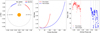 |
Fig. 1 Left: phase coverage of our CRIRES+ pre- and post-eclipse observations. Middle and right: observing conditions showing the variation of airmass and mean signal-to-noise ratio (S/N) with orbital phase. Vertical grey bands denote cloud-affected regions. |
3 A search for atmospheric species
3.1 Model spectra
To search for chemical species in the atmospheres of exoplanets and place quantitative constraints on atmospheric properties, both the cross-correlation and likelihood approaches require spectral templates. Therefore, for our analysis, we computed the 1D atmospheric models using IRRADIATOR (Gibson et al. 2022), where we defined 80 atmospheric layers equally spaced in log pressure from 10−8 bar to 100 bar and computed the T – P profile at each layer using the parametric model from Guillot (2010) with four input terms Tirr (irradiation temperature), κIR (mean infrared opacity), γ (ratio of visible-to-infrared opacity) and Tint (internal temperature). Next, we set the volume mixing ratios (VMRs), χspecies, for each species of interest at each layer. These are either given as free parameters, that is, the species are assumed to be well-mixed, or computed using FASTCHEM2 (version 3.1.1, Stock et al. 2018, 2022; Kitzmann et al. 2024) using an additional free parameter to specify the metallicity (relative to solar) and C/O ratio, where we adjust both C and O abundances to have a desired ratio but preserve their sum. We compute the emission by integrating through the atmosphere for every point in the wavelength grid, assuming blackbody emission from the deepest layer. The spectra are calculated across a wavelength range of 1800–2850 nm at a constant resolution of R = 200 000. In our atmospheric models, we accounted for the opacity contributions from chemical species prominent in the atmospheres of UHJs at near-infrared wavelengths (e.g. Snellen et al. 2010; Birkby et al. 2013; Nugroho et al. 2020a; Brogi et al. 2023). For atomic and molecular absorption, we used the high-resolution pre-computed opacity grids provided by petitRADTRANS3 (version 2.7.7, Mollière et al. 2019, 2020) and also included collision-induced opacity due to H2-H2 and H2- He and bound-free and free-free absorption from H−, using the cross-sections from Gray (2005) and Abel et al. (2011). Additionally, we incorporated a parameterised cloud deck pressure (Pcloud), assuming infinite opacity below the atmosphere. Lastly, since data pre-processing methods such as SYSREM can alter the underlying planet signal, applying these same processing steps to our forward models as we do to the data is necessary. Thus, we implemented the model filtering technique introduced by Gibson et al. (2022), which makes use of the output matrices U and W (Sect. 2), containing the column and row vectors u and w for each SYSREM iteration. Before applying this technique, we convolved our model emission spectra with a broadening kernel with a standard deviation of Wconv , followed by linear interpolation to match the 2D wavelength grid of our data. After this, we Doppler shifted this model to a planetary velocity, υp , for each order:
 (2)
(2)
where Kp , ϕ, υsys and υbary are the radial velocity semi-amplitude of the planet’s orbit, orbital phase, the systemic velocity offset and barycentric velocity, respectively. This produced a 3D shifted forward model that was then filtered using the SYSREM basis vectors via the procedure outlined in Gibson et al. (2022).
In summary, we specify our 1D atmosphere using the parametric model from Guillot (2010) and two different chemical regimes, assuming either that the species of interest are well- mixed (constant VMRs with altitude) or by using FASTCHEM to compute the chemical profiles after specifying a C/O ratio and metallicity. We applied various combinations of these parametrisations to our cross-correlation and retrieval analyses, which we discuss in more detail in Sect. 4. The model spectrum (constant VMRs) and corresponding T–P profile are shown in Fig. 3.
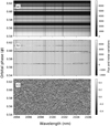 |
Fig. 2 Data pre-processing steps, applied to a single order: (a) raw spectra, (b) cleaned and blaze corrected spectra, and (c) residual spectra after division by the median spectrum and subtraction of the SYSREM model (shown weighted by the uncertainties). We note that the blaze correction does not work well for cloud-affected frames, resulting in some horizontal structure (residuals) in these regions (the last two panels). However, they only have a minimal impact on our retrievals. |
3.2 Injection and recovery tests
Before performing a retrieval analysis (outlined in Sect. 4) using our forward model, we conducted injection and recovery tests to ensure the pre-processing and filtering steps did not alter the underlying planet signal. We injected an atmospheric model containing CO, H2O, and Fe with a negative value of the expected Kp and performed our retrieval analysis on the injected data. We found the retrieved model parameters and T–P profiles to be in agreement with the injected values (see Appendix A). Additionally, although the cloud-affected frames effectively contain weaker signals due to low S/N and could be filtered out, given the already limited phase coverage and data, we chose not to exclude these frames. To ensure their inclusion did not bias the results, we ran retrievals (Sect. 4) with and without the cloud-affected frames. We found the retrieved parameters and T – P profiles to be consistent within ≈1σ (see Appendix B). Although including these frames introduced small changes to the temperature gradient and irradiation temperature (Tirr), they did not impact the overall results.
3.3 Cross-correlation
After removing the stellar and telluric lines from our data using SYSREM, the remaining data is dominated by noise (panel c of Fig. 2). To extract the planetary signal, we employ the traditional cross-correlation technique (e.g. Snellen et al. 2010) and generate the cross-correlation function (CCF) by summing the product of the residual data (fi) and the shifted (+filtered) model (mi), weighted on the variance of the data (σi) over both spectral order and wavelength:
 (3)
(3)
This produces a cross-correlation array of phase vs Δυsys, referred to as the cross-correlation map, where Δυsys represents the residual velocity shift relative to the stellar rest frame after correcting for systemic and barycentric velocities4. For strong planetary signals, the CCF will trace out the predicted radial velocity with phase in the CC-map, allowing us to confirm the presence of atmospheric species in exoplanets. However, the strength of the cross-correlation (CC) signal is often much weaker, and we need to integrate the cross-correlation map over a range of predicted planetary velocities (υp). Since the exact value for the radial velocity semi-amplitude (Kp) is unknown and to evaluate noise, we select a range of Kp values close to the predicted value from radial-velocity measurements (Table 2) and shift the CCF to a new planetary velocity (according to Eq. (2)) and then integrate over time to produce a Kp–∆υsys map. Integration helps isolate the source of the signal in velocity space, and we can be confident of the detection of species in the atmosphere.
The final step in securing the spectroscopic detection of the exoplanet is to determine the significance level of the signal, which measures the signal amplitude. There are several ways to do this (see, e.g. Snellen et al. 2010; Birkby et al. 2013). We subtract the Kp–Δυsys map by the mean in regions away from the peak before dividing through by the standard deviation (Brogi et al. 2012, 2018). Since it is difficult to interpret the significance of these values statistically due to the arbitrary selection of this region, we utilise the likelihood distribution (see Sect. 4.1) of our model scale factor, α, to compute the detection significance, similar to the approach of Gibson et al. (2020), which we discuss in the following sections.
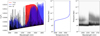 |
Fig. 3 Left panel: best-fit model spectra (constant VMRs) of MASCARA-1b with contributions from the chemical species shown individually. Middle and right panels: the parametric T–P profile from Guillot (2010) and combined contribution function. |
3.4 Cross-correlation results
Following the procedure outlined in the previous section, we searched for individual species of interest by cross-correlating our data with a filtered model emission spectrum using the bestfitting model parameters from our atmospheric retrieval (see Sect. 4). We calculated the Kp–Δυsys maps by shifting the CCFs to the rest frame of the planet over a range of Kp and Δυsys from −300 to +300 km s−1, in steps of 0.3 and 0.2 km s−1, respectively, and summed over time. To estimate the detection significance (sometimes referred to as signal-to-noise, e.g. Brogi et al. 2018), we divided the Kp–Δυsys maps by their standard deviation calculated by avoiding the area ±50 km s−1 from the expected planet signal.
In our search for chemical species in the day-side atmosphere of MASCARA-1b, we detected strong emission signatures of CO, H2O and Fe in the pre-eclipse data and CO and H2O in the post-eclipse data (second panel of Fig. 4), respectively. These emission features are also detected at high significance when combining the two nights (middle panel of Fig. 4). Despite the lower S/N of the post-eclipse data, CO and H2O are detected at similar strengths as in the pre-eclipse data. We do not detect iron in the post-eclipse and the combined dataset. The species are detected roughly at the expected Kp and Δυsys, except for the pre-eclipse Fe signal that has a slight offset in both Kp and Δυsys. We discuss our iron detection in more detail in Sect. 5.2. The Kp–Δυsys maps of the individual species and the full atmosphere for the pre-, post- and pre+post datasets are shown in Figures 4 and 5, respectively. The colour bar shows the detection significance5 values computed from the maps and the strong negative values are deep side lobes near the signal. We note that the α method is less sensitive to these choices, offering a more objective and robust assessment of the detection significance. For both datasets, the emission signal for the entire atmosphere is strong and directly observable on the CCF map (see Fig. 6). In addition, we also applied the cross-correlation method to search for 13CO, Mg, CO2, OH, HCN, Si and Ca but no significant detections are found in the Kp–Δυsys maps of the species (see Appendix C).
We emphasise that the detection significance values computed from the maps can change when cross-correlating with the same models due to the arbitrary selection of the noise region. Therefore, we followed the method outlined in Gibson et al. (2020) to evaluate the detection significance. We first computed the log-likelihood distribution (Sect. 4.1) based on the model scale factor, α, conditioned on the optimal values of all atmospheric parameters. Next, we calculated the mean of this distribution and divided it by the standard deviation to determine the “alpha” detection significance. This value indicates how many standard deviations the maximum signal deviates from an alpha of 0, corresponding to a null signal. Because the alpha detection significance is based on likelihood, the results are more objective, less arbitrary (i.e. require fewer assumptions) and provide a more conservative representation of the data. The penultimate panel of Fig. 4 shows a plot of the detection significance computed from the Kp–Δυsys maps and the alpha detection significance of the detected species for the datasets.
Parameters for MASCARA-1 system.
4 Atmospheric retrievals
While cross-correlation allows us to obtain detections of chemical species in the atmospheres of exoplanets, it does not provide quantitative information about the atmospheric properties. Additionally, this technique does not allow direct comparisons between observations and atmospheric models. However, recent advances in high-resolution Bayesian methods (e.g. Brogi & Line 2019; Gibson et al. 2020) have allowed us to “map” crosscorrelation values of a given atmospheric model to a likelihood value. This will enable us to perform atmospheric ‘retrievals’ that help constrain properties such as the temperature profile, chemical and/or elemental abundances, and subsequent products like the atmospheric C/O ratio and metallicity. We apply the same retrieval framework described in Ramkumar et al. (2023), which follows the approach of Gibson et al. (2020, 2022), to estimate the chemical composition and thermal structure of MASCARA-1b. We briefly outline our retrieval setup and present our results in the following sections.
4.1 Retrieval framework
To perform our retrieval analysis on the datasets, we computed our forward model, mi , by taking into account the atmospheric model parameters, θ = {κIR, γ, Tirr, Tint, Pcloud, χspecies×Nspecies}, the broadening kernel width {Wconv}, planetary velocities {Kp , Δυsys}, and the scaling factors for the model ({α}) and noise ({β}). The forward model was then filtered using the procedure outlined in Gibson et al. (2022). Finally, the log-likelihood for a given set of model parameters is computed as follows:
 (4)
(4)
with
 (5)
(5)
where, fi and σi are the data and the standard deviation, respectively. Assuming uniform priors (defined over linear or logarithmic parameter spacing, as listed in Tables 3 and 4), we compute the log-posterior by computing the log-prior and then adding the log-likelihood (i.e. Eq. (4)), which was folded into a Markov chain Monte Carlo (MCMC) framework to retrieve posterior distributions of the model parameters for each dataset. We use a Differential-Evolution Markov Chain (DEMC) (Ter Braak 2006; Eastman et al. 2013), running an MCMC chain with 192 walkers, with a burn-in length of 200 and a chain length of 300. This setup results in 96 000 samples, of which 38 400 are discarded. To assess convergence, we apply the Gelman-Rubin statistic (Gelman & Rubin 1992) after splitting the chains into four separate groups.
For our retrieval analysis, we focus on the chemical species detected in the day-side atmosphere of MASCARA-1b. Therefore, the number of atmospheric species under consideration, Nspecies , is three (i.e. CO, H2O, and Fe). However, we note that this parameter may vary in different MCMC runs as we also include other C- and O-bearing species for the sake of completeness, in which case, the value of Nspecies is mentioned within parentheses (e.g. Sect. 5.3). We fixed Tint to be 100 K and α to be 1 in the model fits, and although α is fixed in the retrievals, it can be easily computed within the likelihood mapping, post-MCMC. That is, defining alpha as a free parameter in the likelihood rather than incorporating it into the model means we can quickly compute the conditional likelihood as a function of alpha from a fixed cross-correlation map. The last panel of Fig. 4 shows the conditional likelihood distribution of α of the detected species for the pre, post and pre+post datasets.
4.2 Retrieval results
We employ two approximations to describe the atmospheric chemical composition of MASCARA-1b in our retrieval setup. The first approach involves a free retrieval of the mixing ratios for the species, while the second approach uses FastChem (Stock et al. 2018, 2022; Kitzmann et al. 2024) to calculate the abundances self-consistently. The pre-eclipse data are analysed in Ramkumar et al. (2023) and we refer the reader there for a detailed discussion. The retrieved T–P profiles for the two approximations are over-plotted in Fig. 7 and the corresponding posterior distributions are plotted in Figures D.1 and D.2, respectively.
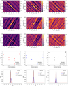 |
Fig. 4 Detection of individual species in the atmosphere of MASCARA-1b. Top, second and middle panels: Kp–∆υsys maps for the pre-eclipse, post-eclipse and pre+post datasets. Penultimate panel: detection significance computed using two ways: α-method is less sensitive to deep side lobes and is more objective (see text and Sect. 4). Bottom panel: conditional likelihood distribution of α. |
 |
Fig. 5 Kp–Δυsys maps of the combined CO, H2O and Fe detection in the atmosphere of MASCARA-1b for the pre-, post- and pre+post eclipse datasets. The atmospheric model used for the cross-correlation has combined contributions from the species and a thermal inversion as discussed in Sect. 3.1. The white dotted lines mark the detection peak, and the colour bar shows the detection significance computed from maps. The corresponding alpha detection significance and the conditional likelihood distribution of α are plotted in Fig. 4. |
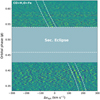 |
Fig. 6 Cross-correlation map for CO+H2O+Fe model, tracing out the planet signal throughout the observed phases. The dashed lines on either side of the CCF trail show the expected planet radial velocity (offset by ±25 km s−1), and the horizontal dashed lines indicate the secondary eclipse. The grey space between the end of our pre-eclipse observations and the start of the eclipse denotes phases at which no data were taken. |
4.2.1 Free retrieval
We begin the retrieval process with a “free-retrieval” paradigm that assumes constant mixing ratios with altitude and uses the parametric model from Guillot (2010). The retrieval parameters and their prior ranges for the datasets are listed in Table 3. For the pre-eclipse, post-eclipse, and joint analysis (pre+post), we place bounded constraints on the abundance of H2O while obtaining lower limits on CO and Fe as their retrieved volume mixing ratios approach the upper bounds of the prior distribution6. We did not detect Fe in the post-eclipse and combined datasets but obtained its 1σ lower limit as log10(χFe) > −4.97 for the latter and did not constrain it in the post-eclipse data. Despite the difference in signal-to-noise between the two datasets, the retrieved parameters for the post-eclipse (shown in blue in Fig. D.1) are consistent with the pre-eclipse values, though with slightly lower precision. When we combine the two nights of CRIRES+ data (shown in black in Fig. D.1), the abundance constraints are consistent with the pre- and post-eclipse sequences. However, they are not more precise than those provided by the pre-eclipse data alone, suggesting that the post-eclipse data contributed little new compositional information. We conclude that the precision is dominated by some degeneracies in the model that are not constrained at those wavelengths. Additionally, it is possible that the planet’s radial velocity trail is not perfectly sinusoidal for all species, which could introduce limitations when combining datasets if a suboptimal model is used. Nevertheless, combining the datasets enabled precise constraints on the planetary velocities (Kp, Δυsys). Overall, the abundances derived from our free-retrieval setup are consistent across the two datasets (pre-eclipse and post-eclipse) as well as the joint analysis (pre+post), with CO dominating relative to H2O on the day-side of MASCARA-1b. However, this does not necessarily imply a carbon-rich atmosphere, as other oxygen-bearing species may influence the interpretation of the C/O ratio (see Sect. 5.1).
Lastly, as noted in Sect. 2, we use 15 SYSREM iterations for our cross-correlation and retrieval analysis presented in this work. While this number is arbitrary, we re-run the analysis with different values of SYSREM for the post-eclipse and combined dataset. The results of this analysis are shown in Figs. E.1 and E.2. We find that using N = 5,10 and 20 iterations give us consistent results for the post-eclipse dataset, whereas N = 20 filtered out some of our exoplanet signal for the pre-eclipse (Ramkumar et al. 2023, Fig. 10) and combined datasets.
4.2.2 Chemical equilibrium
For our retrievals assuming chemical equilibrium, we find that the H2O, H2 and H abundances change quite drastically with altitude in this temperature regime (e.g. right panel of Fig. 7). Therefore, instead of retrieving the individual gas volume mixing ratios, we used FASTCHEM (version 3.1.1, Stock et al. 2018, 2022; Kitzmann et al. 2024) to calculate the abundances of chemical species. This chemical regime is preferred over a well- mixed model, as the latter is known to break down for ultra-hot Jupiters, where strong altitude-dependent variations in composition occur. The results of this analysis (i.e. assuming chemical equilibrium) are shown in Fig. D.2, and the marginalised distributions for each parameter and dataset are summarised in Table 4. We placed bounded constraints on the planetary velocities and the T–P profile parameters for the two datasets and the joint analysis. The retrieved temperature profiles under this setup are over-plotted in Fig. 7 (middle panel). Similar to the free-retrieval setup, constraints on the retrieved parameters for the post-eclipse data remain consistent with the pre-eclipse values, although less precise. In addition, combining the pre-and post-eclipse data provides consistent constraints, albeit weighted more in favour of the pre-eclipse data that appears to be driving these inferences. The retrieved values for the T–P profile parameters between the two retrieval frameworks remain consistent for the individual datasets and the joint analysis (pre+post) within ≈1.1σ.
Lastly, in our retrieval framework, H− bound-free and free-free opacities are included in the chemical equilibrium retrievals but not the free-chemistry retrievals. While the former is less relevant in the K-band, omitting free-free opacity in the free-chemistry retrieval does not significantly affect our results. To verify this, we re-computed our best-fit model emission spectra (assuming chemical equilibrium) with and without the H− free-free opacity (and CIA) and found that the relative flux difference is ∼10−5. This indicates that although H− free-free opacity is present, its impact on the overall emission spectra in the observed K-band wavelength range (1921–2472 nm) is minimal, suggesting that the omission of H− opacities in the free retrievals does not significantly affect the model outcomes for this wavelength range.
Parameters recovered for the combined fits (CO+H2O+Fe) of MASCARA-1b under the free-retrieval (FR) setup.
Parameters recovered for the combined fits (CO+H2O+Fe) of MASCARA−1b under the chemical equilibrium (CE) setup.
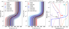 |
Fig. 7 Left and middle panel: retrieved T–P profiles (Guillot 2010) for the pre-eclipse (red), post-eclipse (blue) and pre+post (black) datasets under the free-retrieval and chemical equilibrium setups. The red, blue and grey shading marks the 1σ and 2σ recovered distribution computed from 10 000 samples from the MCMC for both regimes. Right panel: the atmospheric structure for the post-eclipse data from the best-fitting chemical model. The volume mixing ratio profiles for the continuum and detected species are shown as dashed lines (calculated using FASTCHEM), with the parametric T–P profile shown as a solid blue line. |
5 Discussion
5.1 Chemistry of MASCARA-1b
The composition (elemental abundances) of exoplanets, especially of highly irradiated gas giants (e.g. UHJs), can provide clues about the planetary formation and migration histories within the protoplanetary disk (Öberg et al. 2011) via diagnostics like the bulk metallicity and the C/O ratio. Here, we infer the chemistry of MASCARA-1b in terms of the atmospheric C/O and metallicity obtained from our retrieval frameworks. These quantities can be derived from the inferred gas abundances or fitted directly from chemical equilibrium model fits. The former becomes invalid for UHJs due to significant altitude-dependent variations in chemical composition (e.g. Fig. 7), highlighting the need to incorporate vertical chemical equilibrium when interpreting atmospheric properties.
Nonetheless, to assess potential biases introduced by the well-mixed assumption, we compute the free-retrieval based C/O and metallicity of MASCARA-lb derived from our retrieved gas abundance as follows:
 (6)
(6)
and
![Mathematical equation: $[{\rm{M}}/{\rm{H}}] = {\log _{10}}\left[ {{{2{n_{{\rm{CO}}}} + {n_{{{\rm{H}}_2}{\rm{O}}}} + {n_{{\rm{Fe}}}}} \over {2{n_{{{\rm{H}}_2}}}{{\left[ {\left( {{n_{\rm{O}}} + {n_{\rm{C}}} + {n_{{\rm{Fe}}}}} \right)/{n_{\rm{H}}}} \right]}_ \odot }}}} \right]$](/articles/aa/full_html/2025/03/aa53520-24/aa53520-24-eq50.png) (7)
(7)
We assume that CO and H2O are the dominant carbon- and oxygen-bearing molecules in the atmosphere of MASCARA-1b and compute the planetary metallicity by normalising the elemental abundances relative to hydrogen (the numerator in Eq. (7)), relative to that in the Sun (the denominator in Eq. (7)). The solar elemental abundances are taken from Asplund et al. (2009) and the median values of these derived quantities for the datasets are listed in Table 3. The derived metallicities for the pre-eclipse and combined datasets are consistent with the solar value within 1σ and are broadly consistent with the stellar value within their uncertainties. For the post-eclipse data, despite the strong CO detection, the derived [M/H] appears lower than that of the pre-eclipse. This difference is likely driven by the absence of detectable iron in the post-eclipse data, combined with the slightly weaker H2O detection and/or constraint. However, the pre- and post-eclipse metallicities remain statistically consistent.
Looking at the derived C/O ratios, we obtain very precise constraints with  ,
,  and
and  for the pre-, post- and combined datasets. While there are no reported/measured values of the C/O ratio for the host star, MASCARA-1, the derived values are all markedly super-solar and are only constrained by our detection of CO and H2O, assuming that every bit of C and O is within these molecules. However, this assumption could be incomplete. Qualitatively, if a significant portion of the oxygen is present in other species, such as OH or atomic oxygen, due to thermal dissociation of H2O, it could influence the C/O ratio we are measuring. OH is expected to be present on the day side of MASCARA-1b, as it has been detected in colder planets such as WASP-121b and WASP-76b (Smith et al. 2024b; Landman et al. 2021; Gandhi et al. 2024; Weiner Mansfield et al. 2024). However, since K-band CRIRES+observations are not sensitive to OH lines and atomic oxygen is not observable in the near-infrared, our current retrievals may not fully account for these species. Therefore, we included potential C- and O-bearing species that exhibit sharp spectral lines in this wavelength setting but were not detected (e.g. OH, 13CO, HCN and CO2; here Nspecies = 7), in our free-chemistry retrieval and find that the inclusion of these species does not change the derived C/O, which remains super-solar. Additionally, similar to Brogi et al. (2023), if we account for missing oxygen by assuming atomic O with a VMR of 10−3 we indeed obtain a lower C/O≈0.6, although we are unable to provide a precise estimate of uncertainty for this value. Overall, our free-retrieval-based results strongly favoured a H2O-depleted model over one with a similar abundance of CO and H2O, thereby driving the C/O towards 1 resulting in precise constraints.
While the free-chemistry model offers flexibility by allowing the gas volume mixing ratios to be retrieved individually, the assumption of a well-mixed atmosphere does not accurately reflect the vertical variation in chemical composition, particularly for highly irradiated gas giants. This can lead to biases in the elemental abundance estimates (e.g. Brogi et al. 2023; Ramkumar et al. 2023). Therefore, we fit directly for the C/O ratio and metallicity derived from chemical equilibrium fits (see Table 4 and Fig. D.2) using FastChem. This results in a  ,
,  and
and  for the pre-, post-, and pre+post eclipse datasets, respectively. The retrieved values are all consistent with the solar value within ≈1.1–2σ and the combined dataset provides slightly tighter constraints on the retrieved values than the individual datasets. In addition, the post-eclipse seems to constrain the C/O ratio better than the pre-eclipse, though the difference is negligible. This could be because the uncertainties remain consistent across all datasets, as suggested by our injection-recovery tests (see Appendix A) where the injected and recovered values for both a constant-with-altitude abundance and equilibrium chemistry modelling setups are in good agreement. Nevertheless, we speculate that the uncertainties in these parameters are likely dominated by degeneracies in the model and the wavelength range of the observations, as well as the limitations of our 1D models that do not account for 3D effects such as spatial inhomogeneities in the planet’s atmosphere. These factors may contribute to the consistency of the C/O constraints despite the lower data quality of the post-eclipse sequence. Moreover, although the metallicity prior in our chemical equilibrium retrieval is relatively narrow, once we broaden the metallicity constraints (from 0.001 to 1000x solar), the retrieved C/O ratio remains consistent for the post-eclipse data and the joint analysis. However, we find a strong correlation between C/O and metallicity for the pre-eclipse data (see Fig. D.3), leading to inconsistencies in the retrieved value. While this does not alter our overall conclusions, it highlights an important degeneracy we aim to explore further. Lastly, similar to our free-chemistry analysis, for completeness, we also included opacities for OH, CO2 and HCN in our equilibrium chemistry retrievals and find that the inclusion of these species did not change the retrieved C/O value, which remains consistent with the solar value within ≈1σ.
Overall, our results indicate that the atmosphere of MASCARA-1b has a C/O ratio consistent with the solar value, with the chemical equilibrium retrieval providing more realistic and conservative constraints. While it would be interesting to frame the planet’s chemistry in terms of the chemistry of its parent star, the C/O ratio of MASCARA-lb alone is inconclusive in determining its formation as there are no reported or measured values of the C/O ratio for the host star, MASCARA-1. Figure 8 highlights the diversity of C/O ratios among hot and ultra-hot Jupiters using ground-based high-resolution observations. Most planets in the sample exhibit C/O ratios near or above the solar value, with the observed spread in the reported values reflecting the diversity of formation and migration pathways. MASCARA-lb adds to this population with ratios retrieved from pre-, post-, and combined datasets, all consistent with the solar value, making it a valuable addition to the sample of UHJs with well-constrained C/O ratios. While future observations could further refine these constraints, offering new insights into the planet’s chemical inventory and its formation and migration history, it also underscores the challenges in interpreting these ratios in isolation since carbon and oxygen measurements alone are insufficient to determine the origin of a gas-giant planet due to the intrinsic degeneracies in the planet-building gas and solid compositions (Mordasini et al. 20l6).
Recent studies by Lothringer et al. (2021) and Chachan et al. (2023) elucidated the diagnostic power of refractory elements such as Fe, Mg, Si, and Ca, and introduced the concept of the refractory-to-volatile ratio – the abundance of refractory elements like iron relative to volatile species such as CO and H2O – as a valuable tool for tracing the formation and migration pathways of hot and ultra-hot Jupiters. This ratio provides a framework for predicting how a planet’s solid-to-gas ratio and accretion location within the protoplanetary disk influence its atmospheric composition and has very recently been applied to high-resolution observations of the ultra-hot Jupiter WASP-121b, enabling the exploration of potential formation and migration pathways for such planets (Pelletier et al. 2025; Smith et al. 2024b). In the case of MASCARA-lb, our pre-eclipse detection of iron allows us to estimate the refractory-to-volatile ratio within this framework. Assuming that the Fe signal is not spurious (see Sect. 5.2), we derive the refractory-to-volatile ratio to be ![Mathematical equation: $[{\rm{R}}/{\rm{V}}] = 0.32_{ - 1.49}^{ + 1.17}$](/articles/aa/full_html/2025/03/aa53520-24/aa53520-24-eq57.png) from our free-chemistry retrievals. However, it is important to note that attributing the entire refractory inventory to Fe alone or the volatile inventory solely to CO and H2O likely introduces significant bias, as it excludes contributions from other important rock- and ice-forming elements. The non-detections of other refractory (e.g. Mg, Si) and potential volatile (e.g. OH and atomic O) species, partly due to the scarcity of strong spectral lines in the observed wavelength range, could lead to an incomplete representation of refractory and volatile content. Furthermore, our retrieved ratios are derived assuming a constant-with-altitude modelling regime. For these reasons, we choose not to over-interpret the derived refractory-to-volatile ratio and emphasise the need for future observations to better constrain the inventory of both refractory and volatile species in MASCARA-1b.
from our free-chemistry retrievals. However, it is important to note that attributing the entire refractory inventory to Fe alone or the volatile inventory solely to CO and H2O likely introduces significant bias, as it excludes contributions from other important rock- and ice-forming elements. The non-detections of other refractory (e.g. Mg, Si) and potential volatile (e.g. OH and atomic O) species, partly due to the scarcity of strong spectral lines in the observed wavelength range, could lead to an incomplete representation of refractory and volatile content. Furthermore, our retrieved ratios are derived assuming a constant-with-altitude modelling regime. For these reasons, we choose not to over-interpret the derived refractory-to-volatile ratio and emphasise the need for future observations to better constrain the inventory of both refractory and volatile species in MASCARA-1b.
Nevertheless, UHJs present a tremendous opportunity to diagnose planet formation histories by revealing a wealth of volatile and refractory species in their atmospheres. Combining optical and near-infrared high-resolution emission spectroscopy datasets should provide interesting constraints on refractory-to-volatile elemental ratios for irradiated gas giants.
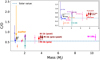 |
Fig. 8 Planetary mass versus C/O ratio for hot and/or ultra-hot Jupiters with constrained abundances of C- and O-bearing species from ground-based high-resolution observations. Our retrieved C/O values for MASCARA-1b are shown as diamonds (labelled M-1b). Values for other planets are from previous studies using either free-chemistry retrievals or chemical equilibrium models (see Table F.1). The dashed line indicates the solar C/O value, and Jupiter is included for reference (from Weiner Mansfield et al. 2024). To reduce clutter, the labels for planets excluding MASCARA-1b and WASP-18b are shown in the inset, which provides a zoomed-in view. For clarity, small mass offsets are applied to WASP-121b, WASP-76b, WASP-189b and MASCARA-1b. |
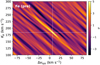 |
Fig. 9 Kp−Δυsys map of the pre-eclipse Fe signal, with the detection significance computed using a region where KP>210 km s−1 and Δυsys< − 40 km s−1, avoiding the planetary signal near the expected Kp and Δυsys. While choosing a different region reduced the detection significance to ≈5σ, Fe remains significantly detected, with the alpha detection significance constrained to be non-zero at more than 4.2σ, supporting the robustness of the Fe signal. |
5.2 Revisiting the iron detection
The detection of iron in the pre-eclipse dataset (Ramkumar et al. 2023) presents an interesting, yet somewhat ambiguous, result. While a prominent peak is found around the consistent Kp and Δυsys in the detection map (see top panel of Fig. 4), albeit a little shifted, we cannot definitively conclude that it is a strong detection of Fe based on our CCF analysis alone. Specifically, the presence of significant negative peaks (e.g. the −6σ feature at a Δυsys≈23 km s−1 and ≈90 km s−1) in the CCF map raises reasons to question the robustness of this detection. We also note that the reported detection significance does not have to be 8σ because the choice of the region used to calculate this is arbitrary and can result in varied values (e.g. Fig. 9). Furthermore, when we perform a free retrieval analysis with a model containing Fe alone, we cannot constrain it, likely because the approach does not account for other species (e.g. CO, H2O) that can mask certain spectral lines or alter the effective line strengths that could potentially weaken the Fe signal. Nonetheless, the presence of a positive CCF peak in our Kp−Δυsys map combined with constraints in our retrieval analysis with all the species seems to indicate that Fe signal in the pre-eclipse data is genuine. In addition, the detection significance derived from the likelihood (alpha value) is constrained to be non-zero at more than 4.2σ (see penultimate panel of Fig. 4), which further boosts our confidence in its detection.
Assuming the pre-eclipse detection is real, the absence of iron in the post-eclipse data becomes particularly intriguing. To explore this, we performed injection-recovery tests with the best-fitting Fe model, injected at a negative Kp. For the pre-eclipse data, the injected and recovered values are in agreement (see Appendix G), with the detection significance computed from the Kp−Δυsys map and the alpha detection significance being ≈10.92σ and ≈8.31σ, respectively. However, we note that the ‘actual’ signal – corresponding to the Fe detection originally observed in the CCF analysis – is not visible in the recovered map. This absence may result from the injected signal adding noise, which can weaken the effective signal, particularly pronounced for weaker detections, such as iron, which has an alpha detection significance of only ≈4.4σ. In contrast, we do not detect iron in the post-eclipse dataset and performing an injection and recovery test yields detection significance and alpha detection significance values of ≈7.73σ and ≈7.53σ, respectively. These values are not significantly different from those of the pre-eclipse dataset; however, they are slightly lower, indicating that the data quality is somewhat reduced, and the sensitivity to iron is consequently diminished. This suggests that the non-detection in the post-eclipse phase could result from the weaker Fe signal falling below the detection threshold due to the slightly poorer signal-to-noise ratio. The non-detection could, therefore, be attributed to the data quality rather than an inherent absence of iron in this phase sequence.
Lastly, to assess whether the inclusion of Fe impacts our inference of other species, we performed retrievals identical to those described in Sect. 4.2, but excluding Fe from the model (i.e. assuming CO and H2O as the only opacity sources). The results are shown in Appendix H. The retrieved temperature profiles with and without Fe are consistent (Fig. 10), suggesting that including iron does not significantly alter the atmospheric structure of MASCARA-1b. This consistency indicates that the model is not artificially forcing iron into the atmosphere by substantially affecting the T–P profile, which might occur if the iron detection were spurious. Furthermore, the absolute abundances of CO and H2O remain unchanged across both models. Our chemical model also predicts iron to exist at these temperatures (right panel of Fig. 10), and the corresponding retrieved T–P profiles remain consistent. Additionally, the abundance retrieved from our free-chemistry retrieval analysis agrees with the predictions from our chemical model. Thus, even if we were to ignore iron, we would still expect to see it in the atmosphere at these temperatures.
5.3 Signatures of atmospheric dynamics
We looked for shifts in the retrieved Kp and Δυsys as proxies for possible atmospheric dynamics, searching for any velocity offsets between the detected species (e.g. Brogi et al. 2023; Cont et al. 2021) or between the pre- and post-eclipse datasets (e.g. Pino et al. 2022). Figure 11 illustrates the 2D posteriors of the detected species for the pre-, post- and pre+post-eclipse datasets. We first search for shifts between the detected species in the individual datasets. For the post-eclipse and pre+post data, CO and the combined species (CO+H2O+Fe) are approximately centred around the expected rest-frame velocity (Δυsys). However, H2O appears slightly shifted in the 2D parameter space but when we examine the 1D marginalised distributions for H2O across the datasets, the results remain consistent with no significant shift. We note that correlations between Kp and Δυsys in the 2D posteriors can be obscured when marginalised, making species-specific shifts challenging to interpret. While H2O seems to be shifted in the 2D space, we have not performed statistical tests to quantify its significance. Therefore, we remain cautious in over-interpreting these shifts based purely on posterior distributions. However, in our analysis of the pre-eclipse data (Ramkumar et al. 2023), tentative evidence for shifts is seen for the Fe feature in both Kp and Δυsys. Specifically, while the cross-correlation analysis shows that the peak (mean) of the map is red-shifted in Δυsys for Fe, the 2D posteriors from the retrieved samples suggest that Fe in general is blue-shifted relative to CO and H2O. If the iron signal is real, this blue shift may indicate that iron is tracing a different dynamical region of the atmosphere, which may also be linked to its non-detection post-eclipse. In addition, to investigate potential differences in dynamics between species, we examine the planetary velocity (υp) as a function of the orbital phase for the detected species in the pre-, post-, and combined datasets (Fig. 12). This plot shows that while the CO and H2O signals exhibit consistent trails across the observed phases, the iron signal appears slightly offset during the earlier phases of the pre-eclipse dataset (see also Fig. I.2 for a zoomed-in version), with the trace overlapping towards the end (i.e. close to the secondary eclipse), where it appears to be more strongly detected.
To further explore these trends and potential longitudinal variations in the atmospheric parameters, we split the pre- and post-eclipse datasets into two subsets based on the orbital phase: phases near quadrature and phases close to the secondary eclipse (see Appendix I). A joint retrieval performed on these subsets indicates that iron is better constrained during the phases close to the secondary eclipse, as corroborated by the Kp−Δυsys maps (Appendix I), and aligns with the trace plot. This raises two possibilities: (i) the stronger detection of iron near the eclipse may be due to localised atmospheric phenomena on the planet, or (ii) when combined with the already weak detection (based on the alpha-detection significance), pre-processing steps like SYSREM is likely getting rid of the signal more efficiently at the lower and/or shorter phases when the planet is more static that could be weakening the iron signal at this phase subset. Both scenarios merit further investigation to disentangle their contributions. Nonetheless, it is intriguing that Fig. 12 combined with the phase-resolved retrieval shows a slightly different trail for iron, which might imply that there are some 3D effects at play that may lead to the non-detection or could in principle lead to a lower signal post-eclipse. That said, we exercise caution in interpreting these features without detailed statistical tests and, therefore, only speculate – underscoring the need for follow-up studies using high-resolution spectroscopy and 3D atmospheric models to explore these phenomena fully.
Following this, we also checked for offsets between the pre-and post-eclipse sequences for each species and found no signatures of atmospheric dynamics (e.g. right panel of Fig. 11). While it is known that different line lists can influence our ability to detect planetary signals, discrepancies in line strengths and positions might affect the S/N (e.g. Webb et al. 2020; Nugroho et al. 2021; Rafi et al. 2024) or retrieved atmospheric properties. Nevertheless, previous analyses, such as that of Gandhi et al. (2020), confirm that the line lists for CO and H2O are appropriate for high-resolution studies up to spectral resolutions of R= 100 000. To assess the robustness of our detections and to determine whether the choice of line list impacts our retrieval results, we performed cross-correlation analysis using the POKAZATEL line list from Exomol for H2O (Polyansky et al. 2018). We found no significant differences between the retrieved parameters or the detection significance computed from the conditional likelihood distribution (see Appendix J) when comparing the POKAZATEL line list with HITEMP 2010 (Rothman et al. 2010), which we use for the results presented in Section 3.3. Additionally, we looked for shifts in the retrieved Kp and Δυsys for H2O alone using two line lists and did not observe any significant shifts in velocity, with all the datasets remaining centred around the expected systemic velocity (see Fig. 13).
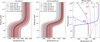 |
Fig. 10 Left and middle panel: retrieved T–P profiles (Guillot 2010) for the pre-eclipse data with the inclusion of iron (i.e. CO+H2O+Fe; red) and without iron (i.e. CO+H2O; black) under the two retrieval setups outlined in Sect. 4.1. The red and grey shading marks the 1σ and 2σ recovered distribution computed from 10 000 samples from the MCMC. Right panel: the atmospheric structure for the pre-eclipse dataset from the best-fitting CO+H2O only model. The volume mixing ratio profiles for the continuum and detected species are shown as dashed lines (calculated using FASTCHEM), with the parametric T–P profile shown as a solid blue line. |
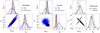 |
Fig. 11 Searching for signatures of atmospheric dynamics. Left and middle panel: posterior distributions for the planetary velocities of CO, H2O and the combined spectrum (i.e. CO+H2O+Fe) for the post-eclipse and pre+post datasets. Right panel: marginalised posterior distributions of the combined atmosphere for the pre- and post-eclipse datasets. |
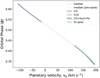 |
Fig. 12 Retrieved planetary orbital velocity (υp) for the detected species from our observations, computed from 10 000 random samples of the MCMC. Dashed lines mark the median, with shaded regions showing 1σ and 2σ contours. For clarity, only the median values (dotted lines) are plotted for the pre+post data. |
5.4 Phase and/or time dependence
Exoplanet atmospheres are inherently 3D structures characterised by dynamic processes, including circulation, chemical mixing, and temperature variations. This is especially true for tidally locked, highly irradiated planets, such as ultra-hot Jupiters, where significant day-to-night temperature gradients can occur. However, our retrieval frameworks currently utilise 1D forward models that assume a globally uniform atmosphere where the atmospheric signal is constant over time. Therefore, it is necessary to exercise caution when interpreting the atmospheric properties retrieved from ID retrievals, as they may not accurately represent the global chemistry of the planet, particularly in cases where phase-dependent variations are expected. For example, recent emission spectroscopy analyses of the UHJ, WASP-33b, detected a phase dependence found via the model scaling parameter, α (e.g. Herman et al. 2022; van Sluijs et al. 2023), and reported that a larger scaling is required to best model the observations after the secondary eclipse. Similarly, Pino et al. (2022) explored atmospheric dynamics in KELT-9b by tracking the planet’s velocity as a function of time using phase-resolved CCFs. Such analyses have demonstrated the power of high-resolution spectroscopy phase curves in probing atmospheric dynamics, temperature gradients, and even potential “3D-ness”.
Our analysis of MASCARA-1b suggests possible variations in the strength of the cross-correlation signal over time, particularly in the pre-eclipse data (see Fig. 6). Notably, the strength of the CCF trail changes at the beginning and end of the observing sequences, with the lower half of the plot (i.e. the start of the observations) showing a diminished trail. This is most likely attributed to the SYSREM pre-processing since de-trending algorithms can remove significant parts of the planet signal. While our filtering technique (Gibson et al. 2022) accounts for these alterations by applying the same pre-processing to the forward model as we do to the data, we will always reduce the signal a little in a phase-dependent way with SYSREM and/or PCA. Nonetheless, the filtering approach works well within our retrieval frameworks, allowing us to recover consistent posteriors with reduced sensitivity to how aggressively the data is filtered until we reach a higher number of SYSREM passes (e.g. Ramkumar et al. 2023, Fig. 10). Additionally, there appears to be a slight dependence on the signal-to-noise, which may also contribute to the variation seen in the CCF. For instance, the pre-eclipse signal disappears towards the end of the sequence, coinciding with a significant increase in airmass and a decrease in S/N. This drop in signal at phases furthest from the eclipse is also expected due to the reduced visibility of the hot day side from the field of view. However, it does not drop off rapidly (see right panel of Fig. 1).
To determine whether the variation in the strength of the CCF trail is solely due to fluctuations in signal-to-noise or if it indicates a physical change in the planet’s signal, we chose not to fix the model scaling α, at 1. Instead, we treated it as a free parameter in our combined (pre+post) retrieval fits. This approach allowed us to examine potential time and/or phase dependence before considering a phase-dependent alpha implementation within the likelihood equation. Upon doing so, we find the retrieved values for α before and after the eclipse to be consistent, with  and
and  . Building on this, we further investigated potential phase-dependent trends by computing a likelihood map as a function of α using a combination of Equations (4) and (5). We began with our cross-correlation map (ϕ vs Δυsys) and calculated it as a function of α (expansion of Eq. (5)). Next, we Doppler-shifted it to the planet rest frame using Eq. (2) (conditioned on the optimal values of all atmospheric parameters). Instead of summing over time, we calculated it for each phase point. This was then used to compute a log-likelihood map as a function of alpha for every frame, which was converted into a likelihood to obtain a conditional likelihood distribution of α, similar to the method outlined in Sects. 3.3 and 4.1 (see also Fig. 4), but for every frame. Lastly, we determined α and its corresponding uncertainties for each phase by calculating the mean and standard deviation of the distribution. A plot of α versus orbital phase for the pre- and post-eclipse datasets is shown in Figure 14. The α values are centred around 1, with no significant trend seen between the two datasets, suggesting that the line contrast is constant over time. However, given the degeneracy between the temperature gradient and chemical abundances (+ continuum), it does not necessarily mean the atmosphere is constant over time. Nonetheless, more sophisticated methods and high-resolution observations may be required to better constrain and probe the phase dependence of the model scaling factor.
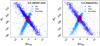 |
Fig. 13 2D posteriors of H2O for the two datasets using the HITEMP and POKAZATEL line lists (see text). |
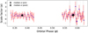 |
Fig. 14 Model scaling factor (α) versus the orbital phase for MASCARA-1b. For visualisation purposes, frames from the individual dataset have been binned together. The α values (blue dots) and their uncertainties for each frame are derived from the conditional likelihood distribution (see text). The black markers show the retrieved median α for the individual datasets. The dark blue points denote outliers corresponding to cloud-affected frames, located within the regions marked by vertical grey bands. |
5.5 Comparison with phase curve measurements
Recent analyses of Spitzer’s 4.5 µm phase curve of MASCARA-1b (Bell et al. 2021; Dang et al. 2025) have measured day-side and night-side temperatures of 3000±100 K and 1300±300 K, respectively, showing a fairly inefficient recirculation, which is consistent with expectations for ultra-hot Jupiters. Building on these findings, we calculated equilibrium temperatures for different heat redistribution scenarios given by the heat redistribution factor, f, as follows:
![Mathematical equation: ${T_{{\rm{p}},{\rm{eq}}}} = {T_ * }{\left( {{{{R_ * }} \over a}} \right)^{{1 \over 2}}}{\left[ {{f \over 4}\left( {1 - {A_{\rm{B}}}} \right)} \right]^{{1 \over 4}}}$](/articles/aa/full_html/2025/03/aa53520-24/aa53520-24-eq60.png) (8)
(8)
where T*, R*, a and AB denote the stellar effective temperature, stellar radius, semi-major axis and the bond albedo, respectively. The heat redistribution factor, f, accounts for the fact that the absorbed energy may not all be re-radiated uniformly over the planet’s surface, with f=1 corresponding to uniform distribution (e.g. full heat redistribution across the planet), f=2 for re-radiation over half the surface of the planet (e.g. day-side only re-radiation) and  corresponding to instant re-emission (Lambertian sphere). For an
  (Dang et al. 2025), we calculate the equilibrium temperature to be ≈2376±35 K, 2826±41 K and 3036±44 K for f= 1, f=2 and
  , respectively. On comparing these with the irradiation temperature from our retrieval analysis, we find that while the results are broadly consistent with f=1, particularly for the free-chemistry setup, given the uncertainties, our results also overlap with f=2, allowing for consistency with any of the heat redistribution scenarios within ≈1σ. However, our uncertainties on the T–P profile remain consistent with the Spitzer phase curve analysis. Additionally, in the context of high-resolution spectroscopy, our analysis of the phase-dependent scaling factor α – which represents variations in line contrast as a function of the orbital phase – reveals no significant trends. This further suggests that we do not observe any substantial changes in the atmosphere of MASCARA-1b as it rotates, likely explaining the consistency in our retrieved parameters between the pre- and post-eclipse datasets. It is also worth noting that the near-symmetric phase coverage of the pre- and post-eclipse datasets may further contribute to the observed consistency. For instance, if the planet’s hotspot exhibits minimal longitudinal offset or its spatial variations are symmetric relative to the substellar point, retrievals from both phases could appear similar even with strong spatial variation. This consistency between pre- and post-eclipse also aligns with the Spitzer phase curve observations, which do not show any significant phase offset (Dang et al. 2025).
6 Conclusions
In this work, we have presented high-resolution emission spectroscopy observations of the UHJ MASCARA-1b with CRIRES+ in the K-band, covering the post-eclipse phases of the planet’s orbit. We applied the standard cross-correlation technique and a Bayesian retrieval framework that includes both pre-eclipse and post-eclipse datasets and learned the following about the thermal and chemical properties of the planet:
In addition to the CRIRES+ pre-eclipse phase-curve observations presented in Ramkumar et al. (2023), we present here an additional night taken two years apart, capturing the planet’s day-side emission in the post-eclipse phases. Using the traditional cross-correlation method, we detected the presence of CO and H2O in the post-eclipse data, with the features also identified at high significance in the joint (pre+post) analysis (Sect. 3.3);
The molecular species are seen as emission signatures through which we also confirmed the presence of a thermal inversion layer in the day-side atmosphere of MASCARA-1b. No significant signature of the chemical species CO2, 13CO, OH, Mg, HCN and CH4 could be detected in our pre-, post-, and pre+post-eclipse data (Sect. 3.3);
The likelihood framework introduced in Gibson et al. (2020, 2022) was applied to obtain quantitative constraints on the atmospheric properties, such as the parametric T–P profile, planetary velocities (Kp, Δυsys), abundances of the species as well as the atmospheric C/O ratio while simultaneously marginalising over the noise properties of the dataset (Sect. 4);
We implemented two different approximations in our retrieval framework to describe the chemical composition of MASCARA-1b’s atmosphere (Sect. 4.1). While our free-chemistry retrievals that assume a well-mixed atmosphere, indicate a super-solar C/O ratio, incorporating a chemical equilibrium model results in a C/O of
 for the post-eclipse data and
  for the joint analysis, both consistent with solar values within ≈1.1–2σ (Sect. 4.2). The chemical equilibrium model, which accounts for altitude-dependent variations in composition, is the preferred model for ultra-hot Jupiters, given their complex atmospheric dynamics;
Despite the difference in signal-to-noise between the pre-and post-eclipse datasets, the retrieved model parameters, under both free-chemistry and chemical equilibrium setups, are consistent with the pre-eclipse values, though less precise. Combining the two nights of the CRIRES+ data enabled slightly tighter constraints on the retrieved parameters than the individual datasets. Overall, the retrieved values for the T–P profile parameters between the two retrieval frameworks remain consistent across the datasets, falling within ≈1.1σ (Sect. 4.2);
We revisit the detection of the Fe signal in our pre-eclipse data (Sect. 5.2) and found no signatures of atmospheric dynamics in the post-eclipse and combined datasets (Sect. 5.3);
A phase-dependent analysis of the scaling factor α showed no significant variation between the pre- and post-eclipse phases, with the retrieved median a values centred around ≈1 (Sect. 5.4);
We find no strong evidence for 3D effects in the atmosphere of MASCARA-1b, and given the large uncertainties on the T–P profile, our findings can be explained by any of the f values and are not in conflict with the Spitzer phase curve (Sect. 5.4). Nonetheless, we note that our observations cover only a subset of the planet’s rotation, which may limit our sensitivity to detecting longitudinal temperature variations or other 3D effects.
While the consistency between pre- and post-eclipse retrievals may not be particularly intriguing from a 3D perspective, it remains interesting that this agreement persists even though the observations were taken two years apart, with the post-eclipse data probing the atmosphere of MASCARA-lb after the planet had rotated by approximately ≈106 degrees compared to the pre-eclipse observations. Future high-resolution observations with broader phase coverage and/or complementary wavelengths could further enhance our understanding of longitudinal and temporal variability in ultra-hot Jupiter atmospheres. Such observations, in synergy with space-based facilities such as the JWST, could help provide critical insights into the chemical and thermal dynamics shaping these extreme planetary environments.
Acknowledgements
We thank the anonymous referee for careful reading of the manuscript and providing helpful comments. This work relied on the observations collected at the European Organisation for Astronomical Research in the Southern Hemisphere under ESO programs 107.22TQ.001 (PI: Gibson) and 112.260X.001 (PI: Gibson, dPI: Ramkumar). We are extremely grateful to the CRIRES+ instrument teams and observatory staff who made these observations possible. S.R. gratefully acknowledges support from the Provost’s PhD Award from Trinity College Dublin. N.P.G is supported by Science Foundation Ireland and the Royal Society in the form of a University Research Fellowship and S.K.N. is supported by JSPS KAKENHI grant No. 22Kl4092. We are grateful to the developers of the NumPy, SciPy, Matplotlib, iPython, corner, petitRADTRANS, FASTCHEM, and Astropy packages, which were used extensively in this work (Harris et al. 2020; Virtanen et al. 2020; Hunter 2007; Perez & Granger 2007; Foreman-Mackey 20l6; Mollière et al. 20l9; Stock et al. 2018, 2022; Astropy Collaboration 2022).
Appendix A Injection-recovery tests
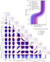 |
Fig. A.1 Summary of our injection tests for pre-, post- and pre+post-eclipse datasets outlined in Sect. 3.2, with the 1D and 2D marginalised posterior distributions of each of our model parameters displayed. The red, blue and black posterior distributions represent the datasets, with the injected values highlighted by horizontal and vertical solid purple lines. The dotted lines show the retrieved median values. Upper right: the retrieved T–P profiles are computed from 10,000 random samples of the MCMC; the solid curves show the median profiles and the shaded regions show the 1σ and 2σ contours. The dashed black curve shows the injected T–P profile. |
Appendix B Additional retrieval analyses including the cloud-affected frames in the post-eclipse data
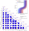 |
Fig. B.1 Free-retrieval results for the post-eclipse data with (red) and without (blue) the inclusion of cloud-affected frames (Sect. 3.2). While excluding these frames slightly improved the Fe constraint, it is still a long-tailed distribution and did not impact the overall conclusions (Fe remains a non-detection). |
Appendix C Additional Kp−Δυsys maps
 |
Fig. C.1 Kp−Δυsγs maps for the non-detected species. Left panels: emission model of each species with the wavelengths covered by CRIRES+ K2166 setting used in this work shown as vertical grey bands. Middle and right panels: the detection maps for the pre-ecl., post-ecl., and combined nights of the CRIRES+ data (Sect. 3.4). The high-resolution opacities were obtained from the following sources: 13CO, CO2 and OH from the HITEMP line list (Rothman et al. 2010), metal opacities from (Kurucz 2018) and HCN opacities from ExoMol database (Harris et al. 2006; Barber et al. 2014). |
Appendix D Atmospheric retrievals of MASCARA-1b
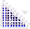 |
Fig. D.1 Summary of our free-retrieval results for the combined atmosphere with the 1D and 2D marginalised posterior distributions of each model parameter displayed within a corner plot. The red, blue and black distributions represent the pre-, post- and pre+post eclipse datasets (Sect. 4.2). |
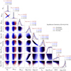 |
Fig. D.2 Same as Figure D.1, but for the chemical retrieval described in Section 4.2.2. |
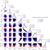 |
Fig. D.3 Same as Figure D.2, but with a broader metallicity prior (from 0.00l to l000x solar). |
Appendix E Consistency between SYSREM iterations on the post-eclipse and pre+post datasets
 |
Fig. E.1 Summary of our free-retrieval results with the 1D and 2D marginalised posterior distributions of the parameters from the MCMC fit. The different colours show the samples obtained using four values for the SYSREM iterations (Sect. 4.2.1). |
Appendix F Ground-based high-resolution measurements of well-constrained C/O ratios
Appendix G Injection and recovery test for Fe
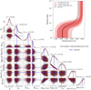 |
Fig. G.1 Results of the injection and recovery test for the pre-eclipse Fe (Sect. 5.2). The red and black posterior distributions represent independent sub-chains of the same MCMC chain, both converging to similar distributions. Upper right: the retrieved T–P profile computed from 10,000 random samples of the MCMC; the solid red curve shows the median profile and the shaded regions show the 1σ and 2σ contours. The dashed black curve shows the injected T–P profile. |
 |
Fig. G.2 Recovered Kp−Δυsys maps of iron for the pre- and post-eclipse datasets. The white dotted lines mark the peak of detection. |
Appendix H Revisiting the pre-eclipse iron detection
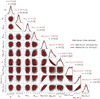 |
Fig. H.1 Results of the free-retrieval for the pre-eclipse dataset with (red) and without (black) the inclusion of Fe as described in Sect. 5.2. |
Appendix I Phase-dependent retrieval
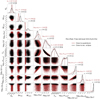 |
Fig. I.1 Results of the joint (pre+post) phase-dependent free-retrieval as described in Sect. 5.2. The subsets of phases close to the quadrature are shown in red and phases close to the eclipse are shown in black. Top right: retrieved T–P profile. |
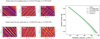 |
Fig. I.2 Left: Kp−Δυsys maps for the iron signal using the phase-dependent retrieval setup. Right: The retrieved planetary orbital velocity (υp) of the detected species for the pre-eclipse data alone, computed from 10,000 random samples of the MCMC. The dashed lines show the median value, and the shaded regions show the 1σ and 2σ contours (see Sect. 5.3). |
Appendix J Plot of alpha detection significance using different line lists for the pre-eclipse, post-eclipse and pre+post datasets
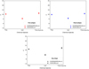 |
Fig. J.1 Plot of alpha detection significance computed from the conditional likelihood distribution (detailed in Sects. 3.3 and 4) using different line lists (see Sect. 5.3) shown for the pre-eclipse, post-eclipse and pre+post datasets. The labels ‘H10’ and ‘H19’ correspond to the HITEMP 2010 and HITEMP 2019 line lists, respectively. |
References
- Abel, M., Frommhold, L., Li, X., & Hunt, K. L. C. 2011, J. Phys. Chem. A, 115, 6805 [NASA ADS] [CrossRef] [Google Scholar]
- Asplund, M., Grevesse, N., Sauval, A. J., & Scott, P. 2009, ARA&A, 47, 481 [NASA ADS] [CrossRef] [Google Scholar]
- Astropy Collaboration (Price-Whelan, A. M., et al.) 2022, ApJ, 935, 167 [NASA ADS] [CrossRef] [Google Scholar]
- Barber, R. J., Strange, J. K., Hill, C., et al. 2014, MNRAS, 437, 1828 [CrossRef] [Google Scholar]
- Bazinet, L., Pelletier, S., Benneke, B., Salinas, R., & Mace, G. N. 2024, AJ, 167, 206 [NASA ADS] [CrossRef] [Google Scholar]
- Bell, T. J., Dang, L., Cowan, N. B., et al. 2021, MNRAS, 504, 3316 [NASA ADS] [CrossRef] [Google Scholar]
- Birkby, J. L., de Kok, R. J., Brogi, M., et al. 2013, MNRAS, 436, L35 [Google Scholar]
- Brogi, M., & Line, M. R. 2019, AJ, 157, 114 [Google Scholar]
- Brogi, M., Snellen, I. A. G., de Kok, R. J., et al. 2012, Nature, 486, 502 [Google Scholar]
- Brogi, M., Line, M., Bean, J., Désert, J. M., & Schwarz, H. 2017, ApJ, 839, L2 [Google Scholar]
- Brogi, M., Giacobbe, P., Guilluy, G., et al. 2018, A&A, 615, A16 [NASA ADS] [CrossRef] [EDP Sciences] [Google Scholar]
- Brogi, M., Emeka-Okafor, V., Line, M. R., et al. 2023, AJ, 165, 91 [NASA ADS] [CrossRef] [Google Scholar]
- Chachan, Y., Knutson, H. A., Lothringer, J., & Blake, G. A. 2023, ApJ, 943, 112 [NASA ADS] [CrossRef] [Google Scholar]
- Cont, D., Yan, F., Reiners, A., et al. 2021, A&A, 651, A33 [NASA ADS] [CrossRef] [EDP Sciences] [Google Scholar]
- Dang, L., Bell, T. J., Shu, Y. Z., et al. 2025, AJ, 169, 32 [NASA ADS] [CrossRef] [Google Scholar]
- Dorn, R. J., Anglada-Escude, G., Baade, D., et al. 2014, The Messenger, 156, 7 [NASA ADS] [Google Scholar]
- Dorn, R. J., Bristow, P., Smoker, J. V., et al. 2023, A&A, 671, A24 [NASA ADS] [CrossRef] [EDP Sciences] [Google Scholar]
- Eastman, J., Gaudi, B. S., & Agol, E. 2013, PASP, 125, 83 [Google Scholar]
- Finnerty, L., Schofield, T., Sappey, B., et al. 2023, AJ, 166, 31 [NASA ADS] [CrossRef] [Google Scholar]
- Finnerty, L., Xuan, J. W., Xin, Y., et al. 2024, AJ, 167, 43 [NASA ADS] [CrossRef] [Google Scholar]
- Flagg, L., Turner, J. D., Deibert, E., et al. 2023, ApJ, 953, L19 [NASA ADS] [CrossRef] [Google Scholar]
- Follert, R., Dorn, R. J., Oliva, E., et al. 2014, SPIE Conf. Ser., 9147, 914719 [Google Scholar]
- Foreman-Mackey, D. 2016, J. Open Source Softw., 1, 24 [Google Scholar]
- Gandhi, S., & Madhusudhan, N. 2019, MNRAS, 485, 5817 [Google Scholar]
- Gandhi, S., Brogi, M., Yurchenko, S. N., et al. 2020, MNRAS, 495, 224 [NASA ADS] [CrossRef] [Google Scholar]
- Gandhi, S., Landman, R., Snellen, I., et al. 2024, MNRAS, 530, 2885 [NASA ADS] [CrossRef] [Google Scholar]
- Gelman, A., & Rubin, D. B. 1992, Statist. Sci., 7, 457 [NASA ADS] [Google Scholar]
- Gibson, N. P., Merritt, S., Nugroho, S. K., et al. 2020, MNRAS, 493, 2215 [Google Scholar]
- Gibson, N. P., Nugroho, S. K., Lothringer, J., Maguire, C., & Sing, D. K. 2022, MNRAS, 512, 4618 [NASA ADS] [CrossRef] [Google Scholar]
- Gray, D. F. 2005, The Observation and Analysis of Stellar Photospheres (Cambridge, UK: Cambridge University Press) [Google Scholar]
- Guillot, T. 2010, A&A, 520, A27 [NASA ADS] [CrossRef] [EDP Sciences] [Google Scholar]
- Guo, B., Yan, F., Nortmann, L., et al. 2024, A&A, 687, A103 [NASA ADS] [CrossRef] [EDP Sciences] [Google Scholar]
- Harris, G. J., Tennyson, J., Kaminsky, B. M., Pavlenko, Y. V., & Jones, H. R. A. 2006, MNRAS, 367, 400 [Google Scholar]
- Harris, C. R., Millman, K. J., van der Walt, S. J., et al. 2020, Nature, 585, 357 [NASA ADS] [CrossRef] [Google Scholar]
- Herman, M. K., de Mooij, E. J. W., Nugroho, S. K., Gibson, N. P., & Jayawardhana, R. 2022, AJ, 163, 248 [NASA ADS] [CrossRef] [Google Scholar]
- Hoeijmakers, H. J., Ehrenreich, D., Kitzmann, D., et al. 2019, A&A, 627, A165 [NASA ADS] [CrossRef] [EDP Sciences] [Google Scholar]
- Holmberg, M., & Madhusudhan, N. 2022, AJ, 164, 79 [NASA ADS] [CrossRef] [Google Scholar]
- Hood, T., Debras, F., Moutou, C., et al. 2024, A&A, 687, A119 [NASA ADS] [CrossRef] [EDP Sciences] [Google Scholar]
- Hooton, M. J., Hoyer, S., Kitzmann, D., et al. 2022, A&A, 658, A75 [NASA ADS] [CrossRef] [EDP Sciences] [Google Scholar]
- Hunter, J. D. 2007, Comput. Sci. Eng., 9, 90 [NASA ADS] [CrossRef] [Google Scholar]
- Jones, A., Noll, S., Kausch, W., Szyszka, C., & Kimeswenger, S. 2013, A&A, 560, A91 [NASA ADS] [CrossRef] [EDP Sciences] [Google Scholar]
- Kaeufl, H.-U., Ballester, P., Biereichel, P., et al. 2004, SPIE Conf. Ser., 5492, 1218 [NASA ADS] [Google Scholar]
- Kanumalla, K., Line, M. R., Weiner Mansfield, M., et al. 2024, AJ, 168, 201 [NASA ADS] [CrossRef] [Google Scholar]
- Kataria, T., Sing, D. K., Lewis, N. K., et al. 2016, ApJ, 821, 9 [NASA ADS] [CrossRef] [Google Scholar]
- Kitzmann, D., Stock, J. W., & Patzer, A. B. C. 2024, MNRAS, 527, 7263 [Google Scholar]
- Kotani, T., Tamura, M., Nishikawa, J., et al. 2018, SPIE Conf. Ser., 10702, 1070211 [Google Scholar]
- Kurucz, R. L. 2018, in Astronomical Society of the Pacific Conference Series, 515, Workshop on Astrophysical Opacities, 47 [NASA ADS] [Google Scholar]
- Landman, R., Sánchez-López, A., Mollière, P., et al. 2021, A&A, 656, A119 [NASA ADS] [CrossRef] [EDP Sciences] [Google Scholar]
- Lesjak, F., Nortmann, L., Yan, F., et al. 2023, A&A, 678, A23 [NASA ADS] [CrossRef] [EDP Sciences] [Google Scholar]
- Lesjak, F., Nortmann, L., Cont, D., et al. 2025, A&A, 693, A72 [NASA ADS] [CrossRef] [EDP Sciences] [Google Scholar]
- Line, M. R., Brogi, M., Bean, J. L., et al. 2021, Nature, 598, 580 [NASA ADS] [CrossRef] [Google Scholar]
- Lothringer, J. D., Barman, T., & Koskinen, T. 2018, ApJ, 866, 27 [NASA ADS] [CrossRef] [Google Scholar]
- Lothringer, J. D., Rustamkulov, Z., Sing, D. K., et al. 2021, ApJ, 914, 12 [CrossRef] [Google Scholar]
- Mace, G., Sokal, K., Lee, J.-J., et al. 2018, SPIE Conf. Ser., 10702, 107020Q [NASA ADS] [Google Scholar]
- Madhusudhan, N., Harrington, J., Stevenson, K. B., et al. 2011, Nature, 469, 64 [NASA ADS] [CrossRef] [Google Scholar]
- Maguire, C., Gibson, N. P., Nugroho, S. K., et al. 2023, MNRAS, 519, 1030 [Google Scholar]
- Maguire, C., Gibson, N. P., Nugroho, S. K., et al. 2024, A&A, 687, A49 [NASA ADS] [CrossRef] [EDP Sciences] [Google Scholar]
- Mollière, P., Wardenier, J. P., van Boekel, R., et al. 2019, A&A, 627, A67 [Google Scholar]
- Mollière, P., Stolker, T., Lacour, S., et al. 2020, A&A, 640, A131 [Google Scholar]
- Mordasini, C., van Boekel, R., Mollière, P., Henning, T., & Benneke, B. 2016, ApJ, 832, 41 [Google Scholar]
- Noll, S., Kausch, W., Barden, M., et al. 2012, A&A, 543, A92 [NASA ADS] [CrossRef] [EDP Sciences] [Google Scholar]
- Nortmann, L., Lesjak, F., Yan, F., et al. 2025, A&A, 693, A213 [NASA ADS] [CrossRef] [EDP Sciences] [Google Scholar]
- Nugroho, S. K., Kawahara, H., Masuda, K., et al. 2017, AJ, 154, 221 [Google Scholar]
- Nugroho, S. K., Gibson, N. P., de Mooij, E. J. W., et al. 2020a, ApJ, 898, L31 [Google Scholar]
- Nugroho, S. K., Gibson, N. P., de Mooij, E. J. W., et al. 2020b, MNRAS, 496, 504 [Google Scholar]
- Nugroho, S. K., Kawahara, H., Gibson, N. P., et al. 2021, ApJ, 910, L9 [CrossRef] [Google Scholar]
- Öberg, K. I., Murray-Clay, R., & Bergin, E. A. 2011, ApJ, 743, L16 [Google Scholar]
- Park, C., Jaffe, D. T., Yuk, I.-S., et al. 2014, SPIE Conf. Ser., 9147, 91471D [NASA ADS] [Google Scholar]
- Parmentier, V., Showman, A. P., & Fortney, J. J. 2021, MNRAS, 501, 78 [Google Scholar]
- Pelletier, S., Benneke, B., Ali-Dib, M., et al. 2023, Nature, 619, 491 [NASA ADS] [CrossRef] [Google Scholar]
- Pelletier, S., Benneke, B., Chachan, Y., et al. 2025, AJ, 169, 10 [NASA ADS] [CrossRef] [Google Scholar]
- Pepe, F., Cristiani, S., Rebolo, R., et al. 2021, A&A, 645, A96 [NASA ADS] [CrossRef] [EDP Sciences] [Google Scholar]
- Perez, F., & Granger, B. E. 2007, Comput. Sci. Eng., 9, 21 [Google Scholar]
- Pino, L., Désert, J.-M., Brogi, M., et al. 2020, ApJ, 894, L27 [Google Scholar]
- Pino, L., Brogi, M., Désert, J. M., et al. 2022, A&A, 668, A176 [NASA ADS] [CrossRef] [EDP Sciences] [Google Scholar]
- Polyansky, O. L., Kyuberis, A. A., Zobov, N. F., et al. 2018, MNRAS, 480, 2597 [NASA ADS] [CrossRef] [Google Scholar]
- Prinoth, B., Hoeijmakers, H. J., Kitzmann, D., et al. 2022, Nat. Astron., 6, 449 [NASA ADS] [CrossRef] [Google Scholar]
- Rafi, S. A., Nugroho, S. K., Tamura, M., Nortmann, L., & Sánchez-López, A. 2024, AJ, 168, 106 [NASA ADS] [CrossRef] [Google Scholar]
- Ramkumar, S., Gibson, N. P., Nugroho, S. K., Maguire, C., & Fortune, M. 2023, MNRAS, 525, 2985 [CrossRef] [Google Scholar]
- Roman, M., & Rauscher, E. 2019, ApJ, 872, 1 [NASA ADS] [CrossRef] [Google Scholar]
- Rothman, L. S., Gordon, I. E., Barber, R. J., et al. 2010, J. Quant. Spec. Radiat. Transf., 111, 2139 [NASA ADS] [CrossRef] [Google Scholar]
- Scandariato, G., Borsa, F., Bonomo, A. S., et al. 2023, A&A, 674, A58 [NASA ADS] [CrossRef] [EDP Sciences] [Google Scholar]
- Smith, P. C. B., Line, M. R., Bean, J. L., et al. 2024a, AJ, 167, 110 [NASA ADS] [CrossRef] [Google Scholar]
- Smith, P. C. B., Sanchez, J. A., Line, M. R., et al. 2024b, AJ, 168, 293 [NASA ADS] [CrossRef] [Google Scholar]
- Snellen, I. A. G., de Kok, R. J., de Mooij, E. J. W., & Albrecht, S. 2010, Nature, 465, 1049 [Google Scholar]
- Stock, J. W., Kitzmann, D., Patzer, A. B. C., & Sedlmayr, E. 2018, MNRAS, 479, 865 [NASA ADS] [Google Scholar]
- Stock, J. W., Kitzmann, D., & Patzer, A. B. C. 2022, MNRAS, 517, 4070 [NASA ADS] [CrossRef] [Google Scholar]
- Talens, G. J. J., Albrecht, S., Spronck, J. F. P., et al. 2017, A&A, 606, A73 [NASA ADS] [CrossRef] [EDP Sciences] [Google Scholar]
- Tamura, M., Suto, H., Nishikawa, J., et al. 2012, SPIE Conf. Ser., 8446, 84461T [NASA ADS] [Google Scholar]
- Tamuz, O., Mazeh, T., & Zucker, S. 2005, MNRAS, 356, 1466 [Google Scholar]
- Ter Braak, C. J. F. 2006, Statist. Comput., 16, 239 [Google Scholar]
- van Sluijs, L., Birkby, J. L., Lothringer, J., et al. 2023, MNRAS, 522, 2145 [NASA ADS] [CrossRef] [Google Scholar]
- Virtanen, P., Gommers, R., Oliphant, T. E., et al. 2020, Nat. Methods, 17, 261 [Google Scholar]
- Webb, R. K., Brogi, M., Gandhi, S., et al. 2020, MNRAS, 494, 108 [NASA ADS] [CrossRef] [Google Scholar]
- Weiner Mansfield, M., Line, M. R., Wardenier, J. P., et al. 2024, AJ, 168, 14 [NASA ADS] [CrossRef] [Google Scholar]
- Wright, J. T., & Eastman, J. D. 2014, PASP, 126, 838 [Google Scholar]
Documentation available at the ESO website http://www.eso. org/sci/software/pipelines/
Documentation: https://newstrangeworlds.github.io/FastChem/
Documentation: https://petitradtrans.readthedocs.io/en/latest/
The expected υsys is zero, as the spectra have already been shifted to the stellar rest frame.
Sometimes referred to as signal-to-noise in the literature (e.g. Brogi et al. 2018).
Our corner plots display the marginalised posterior medians and 1σ confidence interval, but we report 1σ lower limits for posterior distributions against the upper prior.
All Tables
Parameters recovered for the combined fits (CO+H2O+Fe) of MASCARA-1b under the free-retrieval (FR) setup.
Parameters recovered for the combined fits (CO+H2O+Fe) of MASCARA−1b under the chemical equilibrium (CE) setup.
All Figures
|
Fig. 1 Left: phase coverage of our CRIRES+ pre- and post-eclipse observations. Middle and right: observing conditions showing the variation of airmass and mean signal-to-noise ratio (S/N) with orbital phase. Vertical grey bands denote cloud-affected regions. |
| In the text | |
|
Fig. 2 Data pre-processing steps, applied to a single order: (a) raw spectra, (b) cleaned and blaze corrected spectra, and (c) residual spectra after division by the median spectrum and subtraction of the SYSREM model (shown weighted by the uncertainties). We note that the blaze correction does not work well for cloud-affected frames, resulting in some horizontal structure (residuals) in these regions (the last two panels). However, they only have a minimal impact on our retrievals. |
| In the text | |
|
Fig. 3 Left panel: best-fit model spectra (constant VMRs) of MASCARA-1b with contributions from the chemical species shown individually. Middle and right panels: the parametric T–P profile from Guillot (2010) and combined contribution function. |
| In the text | |
|
Fig. 4 Detection of individual species in the atmosphere of MASCARA-1b. Top, second and middle panels: Kp–∆υsys maps for the pre-eclipse, post-eclipse and pre+post datasets. Penultimate panel: detection significance computed using two ways: α-method is less sensitive to deep side lobes and is more objective (see text and Sect. 4). Bottom panel: conditional likelihood distribution of α. |
| In the text | |
|
Fig. 5 Kp–Δυsys maps of the combined CO, H2O and Fe detection in the atmosphere of MASCARA-1b for the pre-, post- and pre+post eclipse datasets. The atmospheric model used for the cross-correlation has combined contributions from the species and a thermal inversion as discussed in Sect. 3.1. The white dotted lines mark the detection peak, and the colour bar shows the detection significance computed from maps. The corresponding alpha detection significance and the conditional likelihood distribution of α are plotted in Fig. 4. |
| In the text | |
|
Fig. 6 Cross-correlation map for CO+H2O+Fe model, tracing out the planet signal throughout the observed phases. The dashed lines on either side of the CCF trail show the expected planet radial velocity (offset by ±25 km s−1), and the horizontal dashed lines indicate the secondary eclipse. The grey space between the end of our pre-eclipse observations and the start of the eclipse denotes phases at which no data were taken. |
| In the text | |
|
Fig. 7 Left and middle panel: retrieved T–P profiles (Guillot 2010) for the pre-eclipse (red), post-eclipse (blue) and pre+post (black) datasets under the free-retrieval and chemical equilibrium setups. The red, blue and grey shading marks the 1σ and 2σ recovered distribution computed from 10 000 samples from the MCMC for both regimes. Right panel: the atmospheric structure for the post-eclipse data from the best-fitting chemical model. The volume mixing ratio profiles for the continuum and detected species are shown as dashed lines (calculated using FASTCHEM), with the parametric T–P profile shown as a solid blue line. |
| In the text | |
|
Fig. 8 Planetary mass versus C/O ratio for hot and/or ultra-hot Jupiters with constrained abundances of C- and O-bearing species from ground-based high-resolution observations. Our retrieved C/O values for MASCARA-1b are shown as diamonds (labelled M-1b). Values for other planets are from previous studies using either free-chemistry retrievals or chemical equilibrium models (see Table F.1). The dashed line indicates the solar C/O value, and Jupiter is included for reference (from Weiner Mansfield et al. 2024). To reduce clutter, the labels for planets excluding MASCARA-1b and WASP-18b are shown in the inset, which provides a zoomed-in view. For clarity, small mass offsets are applied to WASP-121b, WASP-76b, WASP-189b and MASCARA-1b. |
| In the text | |
|
Fig. 9 Kp−Δυsys map of the pre-eclipse Fe signal, with the detection significance computed using a region where KP>210 km s−1 and Δυsys< − 40 km s−1, avoiding the planetary signal near the expected Kp and Δυsys. While choosing a different region reduced the detection significance to ≈5σ, Fe remains significantly detected, with the alpha detection significance constrained to be non-zero at more than 4.2σ, supporting the robustness of the Fe signal. |
| In the text | |
|
Fig. 10 Left and middle panel: retrieved T–P profiles (Guillot 2010) for the pre-eclipse data with the inclusion of iron (i.e. CO+H2O+Fe; red) and without iron (i.e. CO+H2O; black) under the two retrieval setups outlined in Sect. 4.1. The red and grey shading marks the 1σ and 2σ recovered distribution computed from 10 000 samples from the MCMC. Right panel: the atmospheric structure for the pre-eclipse dataset from the best-fitting CO+H2O only model. The volume mixing ratio profiles for the continuum and detected species are shown as dashed lines (calculated using FASTCHEM), with the parametric T–P profile shown as a solid blue line. |
| In the text | |
|
Fig. 11 Searching for signatures of atmospheric dynamics. Left and middle panel: posterior distributions for the planetary velocities of CO, H2O and the combined spectrum (i.e. CO+H2O+Fe) for the post-eclipse and pre+post datasets. Right panel: marginalised posterior distributions of the combined atmosphere for the pre- and post-eclipse datasets. |
| In the text | |
|
Fig. 12 Retrieved planetary orbital velocity (υp) for the detected species from our observations, computed from 10 000 random samples of the MCMC. Dashed lines mark the median, with shaded regions showing 1σ and 2σ contours. For clarity, only the median values (dotted lines) are plotted for the pre+post data. |
| In the text | |
|
Fig. 13 2D posteriors of H2O for the two datasets using the HITEMP and POKAZATEL line lists (see text). |
| In the text | |
|
Fig. 14 Model scaling factor (α) versus the orbital phase for MASCARA-1b. For visualisation purposes, frames from the individual dataset have been binned together. The α values (blue dots) and their uncertainties for each frame are derived from the conditional likelihood distribution (see text). The black markers show the retrieved median α for the individual datasets. The dark blue points denote outliers corresponding to cloud-affected frames, located within the regions marked by vertical grey bands. |
| In the text | |
|
Fig. A.1 Summary of our injection tests for pre-, post- and pre+post-eclipse datasets outlined in Sect. 3.2, with the 1D and 2D marginalised posterior distributions of each of our model parameters displayed. The red, blue and black posterior distributions represent the datasets, with the injected values highlighted by horizontal and vertical solid purple lines. The dotted lines show the retrieved median values. Upper right: the retrieved T–P profiles are computed from 10,000 random samples of the MCMC; the solid curves show the median profiles and the shaded regions show the 1σ and 2σ contours. The dashed black curve shows the injected T–P profile. |
| In the text | |
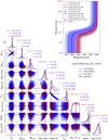 |
Fig. A.2 Same as Fig. A.1 but for a chemical model. |
| In the text | |
|
Fig. B.1 Free-retrieval results for the post-eclipse data with (red) and without (blue) the inclusion of cloud-affected frames (Sect. 3.2). While excluding these frames slightly improved the Fe constraint, it is still a long-tailed distribution and did not impact the overall conclusions (Fe remains a non-detection). |
| In the text | |
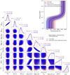 |
Fig. B.2 Same as Fig. B.1 but assuming chemical equilibrium. |
| In the text | |
|
Fig. C.1 Kp−Δυsγs maps for the non-detected species. Left panels: emission model of each species with the wavelengths covered by CRIRES+ K2166 setting used in this work shown as vertical grey bands. Middle and right panels: the detection maps for the pre-ecl., post-ecl., and combined nights of the CRIRES+ data (Sect. 3.4). The high-resolution opacities were obtained from the following sources: 13CO, CO2 and OH from the HITEMP line list (Rothman et al. 2010), metal opacities from (Kurucz 2018) and HCN opacities from ExoMol database (Harris et al. 2006; Barber et al. 2014). |
| In the text | |
|
Fig. D.1 Summary of our free-retrieval results for the combined atmosphere with the 1D and 2D marginalised posterior distributions of each model parameter displayed within a corner plot. The red, blue and black distributions represent the pre-, post- and pre+post eclipse datasets (Sect. 4.2). |
| In the text | |
|
Fig. D.2 Same as Figure D.1, but for the chemical retrieval described in Section 4.2.2. |
| In the text | |
|
Fig. D.3 Same as Figure D.2, but with a broader metallicity prior (from 0.00l to l000x solar). |
| In the text | |
|
Fig. E.1 Summary of our free-retrieval results with the 1D and 2D marginalised posterior distributions of the parameters from the MCMC fit. The different colours show the samples obtained using four values for the SYSREM iterations (Sect. 4.2.1). |
| In the text | |
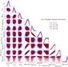 |
Fig. E.2 Same as Fig. E.1 but for the pre+post dataset. |
| In the text | |
|
Fig. G.1 Results of the injection and recovery test for the pre-eclipse Fe (Sect. 5.2). The red and black posterior distributions represent independent sub-chains of the same MCMC chain, both converging to similar distributions. Upper right: the retrieved T–P profile computed from 10,000 random samples of the MCMC; the solid red curve shows the median profile and the shaded regions show the 1σ and 2σ contours. The dashed black curve shows the injected T–P profile. |
| In the text | |
|
Fig. G.2 Recovered Kp−Δυsys maps of iron for the pre- and post-eclipse datasets. The white dotted lines mark the peak of detection. |
| In the text | |
|
Fig. H.1 Results of the free-retrieval for the pre-eclipse dataset with (red) and without (black) the inclusion of Fe as described in Sect. 5.2. |
| In the text | |
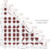 |
Fig. H.2 Same as Fig. H.1 but for a chemical model. |
| In the text | |
|
Fig. I.1 Results of the joint (pre+post) phase-dependent free-retrieval as described in Sect. 5.2. The subsets of phases close to the quadrature are shown in red and phases close to the eclipse are shown in black. Top right: retrieved T–P profile. |
| In the text | |
|
Fig. I.2 Left: Kp−Δυsys maps for the iron signal using the phase-dependent retrieval setup. Right: The retrieved planetary orbital velocity (υp) of the detected species for the pre-eclipse data alone, computed from 10,000 random samples of the MCMC. The dashed lines show the median value, and the shaded regions show the 1σ and 2σ contours (see Sect. 5.3). |
| In the text | |
|
Fig. J.1 Plot of alpha detection significance computed from the conditional likelihood distribution (detailed in Sects. 3.3 and 4) using different line lists (see Sect. 5.3) shown for the pre-eclipse, post-eclipse and pre+post datasets. The labels ‘H10’ and ‘H19’ correspond to the HITEMP 2010 and HITEMP 2019 line lists, respectively. |
| In the text | |
Current usage metrics show cumulative count of Article Views (full-text article views including HTML views, PDF and ePub downloads, according to the available data) and Abstracts Views on Vision4Press platform.
Data correspond to usage on the plateform after 2015. The current usage metrics is available 48-96 hours after online publication and is updated daily on week days.
Initial download of the metrics may take a while.