| Issue |
A&A
Volume 688, August 2024
|
|
|---|---|---|
| Article Number | A8 | |
| Number of page(s) | 26 | |
| Section | Stellar structure and evolution | |
| DOI | https://doi.org/10.1051/0004-6361/202449891 | |
| Published online | 30 July 2024 | |
The accretion burst of the massive young stellar object G323.46−0.08⋆
1
Thüringer Landessternwarte Tautenburg, Sternwarte 5, 07778 Tautenburg, Germany
e-mail: This email address is being protected from spambots. You need JavaScript enabled to view it.
2
INAF – Osservatorio Astronomico di Capodimonte, Salita Moiariello 16, 80131 Napoli, Italy
3
Deutsches SOFIA Institut, University of Stuttgart, 70569 Stuttgart, Germany
4
Department of Physics and Astronomy, University of Exeter, Stocker Road, Exeter EX4 4QL, UK
5
Max Planck Institute for Astronomy, Königstuhl 17, 69117 Heidelberg, Germany
6
ASTRON, Netherlands Institute for Radio Astronomy, Oude Hoogeveensedijk 4, 7991 PD Dwingeloo, The Netherlands
7
Institute of Theoretical Physics and Astrophysics, University of Kiel, Leibnizstraße 15, 24118 Kiel, Germany
8
European Organisation for Astronomical Research in the Southern Hemisphere, Casilla, 19001 Santiago 19, Chile
9
Université Côte d’Azur, Observatoire de la Côte d’Azur, CNRS, Laboratoire Lagrange UMR 7293, Bâtiment H. Fizeau, 06108 Nice Cedex 2, France
Received:
7
March
2024
Accepted:
15
May
2024
Abstract
Context. Accretion bursts from low-mass young stellar objects (YSOs) have been known for many decades. In recent years, the first accretion bursts of massive YSOs (MYSOs) have been observed. These phases of intense protostellar growth are of particular importance for studying massive star formation. Bursts of MYSOs are accompanied by flares of Class II methanol masers (hereafter masers), which are caused by an increase in exciting mid-infrared (MIR) emission. They can lead to long-lasting thermal afterglows of the dust continuum radiation visible at infrared (IR) and (sub)millimeter (hereafter (sub)mm) wavelengths. Furthermore, they might cause a scattered light echo. The G323.46−0.08 (hereafter G323) event, which shows all these features, extends the small sample of known MYSO bursts.
Aims. Maser observations of the MYSO G323 show evidence of a flare, which was presumed to be caused by an accretion burst. This should be verified with IR data. We used time-dependent radiative transfer (TDRT) to characterize the heating and cooling timescales for eruptive MYSOs and to infer the main burst parameters.
Methods. Burst light curves, as well as the pre-burst spectral energy distribution (SED) were established from archival IR data. The properties of the MYSO, including its circumstellar disk and envelope, were derived by using static radiative transfer modeling of pre-burst data. For the first time, TDRT was used to predict the temporal evolution of the SED. Observations with SOFIA/HAWC+ were performed to constrain the burst energy from the strength of the thermal afterglow. Image subtraction and ratioing were applied to reveal the light echo.
Results. The G323 accretion burst is confirmed. It reached its peak in late 2013/early 2014 with a Ks-band increase of ∼2.5 mag. Both Ks-band and integrated maser flux densities follow an exponential decay. TDRT indicates that the duration of the thermal afterglow in the far-infrared (FIR) can exceed the burst duration by years. The latter was proved by SOFIA observations, which indicate a flux increase of (14.2 ± 4.6)% at 70 μm and (8.5 ± 6.1)% at 160 μm in 2022 (2 yr after the burst ended). A one-sided light echo emerged that was propagating into the interstellar medium.
Conclusions. The burst origin of the G323 maser flare has been verified. TDRT simulations revealed the strong influence of the burst energetics and the local dust distribution on the strength and duration of the afterglow. The G323 burst is probably the most energetic MYSO burst that has been observed so far. Within 8.4 yr, an energy of (0.9−0.8+2.5) × 1047 erg was released. The short timescale points to the accretion of a compact body, while the burst energy corresponds to an accumulated mass of at least (7−6+20) MJup and possibly even more if the protostar is bloated. In this case, the accretion event might have triggered protostellar pulsations, which give rise to the observed maser periodicity. The associated IR light echo is the second observed from a MYSO burst.
Key words: accretion, accretion disks / radiative transfer / stars: formation / stars: massive / stars: protostars
Based on observations made with the NASA/DLR Stratospheric Observatory for Infrared Astronomy (SOFIA) under Proposal ID 75_0103 and at the European Organization for Astronomical Research in the Southern Hemisphere under ESO programs ID 077.C-0687(A), 083.C-0582(A), and 290.C-5165(A).
© The Authors 2024
 Open Access article, published by EDP Sciences, under the terms of the Creative Commons Attribution License (https://creativecommons.org/licenses/by/4.0), which permits unrestricted use, distribution, and reproduction in any medium, provided the original work is properly cited.
This article is published in open access under the Subscribe to Open model. This email address is being protected from spambots. You need JavaScript enabled to view it. to support open access publication.
1. Introduction
Episodic accretion events are phases of strongly enhanced mass accumulation during (proto-)stellar growth. These are not restricted to young stars of low and intermediate mass (Hartmann & Kenyon 1996; Audard et al. 2014), but they also occur during the formation of high-mass stars (Caratti o Garatti et al. 2017; Hunter et al. 2017; Stecklum et al. 2021). The energy released during such accretion bursts strongly affects the massive young stellar object (MYSO) and its circumstellar environment in various ways. Heating of the dust in both the circumstellar disk and envelope leads to a temporary increase in the dust continuum emission. Depending on the strength and duration of the burst, this partially or completely affects the spectral energy distribution (SED). The timescales on which the SED changes are wavelength dependent, where different wavelength regions trace different spatial regions (e.g., Contreras Peña et al. 2020). Therefore, accretion bursts provide a unique opportunity for “screening” MYSOs, which are often deeply embedded throughout their formation time.
A specific aspect of MYSO accretion bursts is that their high luminosity leads to the sublimation of volatile substances that were trapped in the ice mantles of dust grains. Thus, for certain molecules, such as methanol in particular, maser emission can occur once the excitation conditions, for example, the specific column density and strong mid-infrared (MIR) radiation field, are satisfied. For this reason, radiatively pumped CH3OH masers (Class II, Menten 1991a; Sobolev et al. 1997; Cragg et al. 2005) are a very good tracer of MYSOs (Breen et al. 2013). These masers will flare during accretion bursts, which makes them a reliable burst alert. Particularly useful is the 6.7 GHz transition (Menten 1991b), as this is usually the brightest. During the burst, the maser spots can be relocated, thus providing information on the local structures such as spiral arms in a disk (see, e.g., Burns et al. 2020).
Even after the burst is over, the far-infrared (FIR) fluxes remain elevated for quite some time, as witnessed for the MYSO G358.93−0.03 burst (Stecklum et al. 2021). This thermal afterglow depends on the local dust distribution and is a record of the history of the burst. Its detection represents an a posteriori confirmation for MYSO bursts, which were not or could not be detected by other means. It allows for the energy release to be constrained, which is fundamental for understanding the triggering mechanisms behind the burst. Until its recent shutdown, the Stratospheric Observatory for Infrared Astronomy (SOFIA, Erickson & Davidson 1993; Young et al. 2012) was the only facility offering the capability to verify the increase in FIR flux caused by the burst, thus allowing for the detection of such an afterglow.
The object G323, which is also known as IRAS15254−5621, is a massive star-forming region. It is located at RA:  , Dec : − 56° 31′23″, J2000. It is covered by various surveys, since it resides in the vicinity of the Galactic center. The red MSX survey (RMS; Lumsden et al. 2013) and the APEX Telescope Large Area Survey of the Galaxy (ATLASGAL; Schuller et al. 2009) revealed the main properties of the region. A bolometric luminosity of L ∼ (1 − 1.3) × 105 L⊙ was derived by integrating its SED (Lumsden et al. 2013). G323 is accompanied by the compact ATLASGAL clump AGAL 323.459−00.079 (Urquhart et al. 2014), considered a massive cluster progenitor (Csengeri et al. 2017) with a mass of ∼600 M⊙ that hosts the MYSO. For this reason, the source is included in the ALMAGAL survey, a large program on ALMA (2019.1.00195.L, PI: S. Molinari), dedicated to studying the evolution of high-mass protocluster formation in the Galaxy. Araya et al. (2005) found blueshifted and redshifted CS (3–2) as well as 13CO (2–1) line wings, indicative of a molecular outflow. A similar signature in the 18CO (2–1) line is observed by the SEDIGISM survey (Yang et al. 2022). However, Guerra-Varas et al. (2023) did not detect an outflow in the SiO (2–1) line and wings of the HCO+ (2–1) line with the APEX telescope. Recently, Ma et al. (2023) identified this clump as a hub for star formation fed by three filaments. For the hub junction, they derived an extent of 2.4 pc × 2.4 pc and a mass of (3072 ± 1200) M⊙.
Associated weak radio continuum emission was first reported by Haynes et al. (1978) and later mapped by Walsh et al. (1998) who did not resolve the source (< 2″). Araya et al. (2005) detected broad radio recombination lines toward this region, indicating the presence of a hypercompact HII region (HCHII). Similar measurements of Murphy et al. (2010), Kim et al. (2018) confirmed this finding. Murphy et al. (2010) also estimated the extinction toward G323, based on the depth of the silicate absorption feature in a low-resolution IRAS spectrum, which amounts to AV = (18 ± 1) mag. The object was observed in the ATOMS survey (ALMA Three-millimeter Observations of Massive Star-forming regions, Liu et al. 2020a) in Autumn 2019. The radio recombination line and the continuum data at 3 mm are used by Zhang et al. (2023) to characterize the HCHII.
The near-kinematic distance of approximately 4.2 kpc is generally preferred, rather than the far distance of 9.3 kpc (Lumsden et al. 2013; Csengeri et al. 2017). Since there is no maser parallax available yet for G323, we re-evaluated its kinematic distance using the radial velocity with respect to the local standard of rest (LSR) of vLSR = −6.72 km s−1 (Proven-Adzri et al. 2019) together with the kinematic model A5 from Reid et al. (2014) which yields a value of (4.08 kpc. This distance is consistent with the largest Gaia-DR2 stellar distances (Bailer-Jones et al. 2018) of up to 3.7 kpc for stars in the foreground of the nebulosity associated with G323. It implies an interstellar extinction of AV ∼ 6 mag according to the model of Amôres & Lépine (2005). The higher Av of Murphy et al. (2010) is reasonable, since the object is located in a star-forming region. Gaia detected a faint source (ID 5883491191298706432, G = 21.45 ± 0.06) close to the position of G323 with an extremely red color BP − RP = 7.29 ± 0.81 (Gaia Collaboration 2021) that points to scattered light from the MYSO. Unfortunately, for such a faint source, the parallax error of Gaia exceeds 1 mas (Cantat-Gaudin et al. 2018), making the distance determination unfeasible.
The massive star-forming region G323 is associated with methanol, water, and hydroxyl masers. The Class II methanol 6.7 GHz transition was first observed by MacLeod et al. (1992). Monitoring of this transition at Hartebeesthoek Radio Astronomy Observatory (HartRAO) revealed an increase in the total flux density from ∼20 Jy in 2011 (Green et al. 2015) to ∼7500 Jy in 2015 (Proven-Adzri et al. 2019), that is, by a factor of ∼430. Interestingly, the decay of the methanol maser, which has been ongoing since then, is characterized by a periodic flux variation with a cycle time of ∼93 d (MacLeod et al. 2021). The first flare evidence was obtained from the brightening of the 6.035 GHz exOH maser (MacLeod et al. 2021). The discovery of the maser flare raises the question whether it is due to an accretion burst, similar to S255IR-NIRS3 (Caratti o Garatti et al. 2017), NGC6334I-MM1 (Hunter et al. 2017, 2018), and G358 (Brogan et al. 2019; MacLeod et al. 2019; Burns et al. 2020; Stecklum et al. 2021). The source is classified as “irregular” in the recent NEOWISE-based variability study of 6.7 GHz maser sources by Song et al. (2023). Their exclusion of the pre-burst WISE epochs prevents the burst detection.
We study the G323 event by combining archival data with recent SOFIA/HAWC+ measurements and the application of TDRT models. So far, the question of the heating and cooling times of YSO dust was treated in a simplified fashion by assuming extreme cases of optical thickness together with energy considerations (Johnstone et al. 2013). The use of the time-dependent radiative transfer code TORUS (Harries 2011; Harries et al. 2019) allows us to estimate the thermal timescales self-consistently. This work represents the first application of TDRT simulations of dust-continuum emission to a real astrophysical object.
The paper is organized as follows. At first, the data obtained by recent observations and from the literature are described in Sect. 2. This is followed by a presentation of the results of the data analysis in Sect. 3. The theoretical part in Sect. 4 contains the radiative transfer (RT) modeling. It starts with the pre-burst static RT modeling. Then, TDRT modeling follows, which predicts the afterglow evolution and main burst parameters for three limiting cases. We draw our conclusions about the burst impact at the end of Sect. 4.4. Sections 5 and 6 evaluate and summarize our findings and put them in the context of current observations of MYSO accretion bursts.
2. Observations and data reduction
2.1. VVV(X) survey imaging
The VISTA Variables in Via Lactea Survey (VVV, Minniti et al. 2010) and its extension VVVX (from 2016 to 2019) are ESO public surveys that were conducted with the 4-m VISTA telescope in the red optical/near-infrared (NIR) domain. They target the Galactic bulge and part of the adjacent plane. Images of the G323 region were retrieved from the VISTA Science Archive. VVV(X) obtained Ks-band imaging in all of their observing epochs of the region. Data for the Z, Y, J and H filters are available only for 2010 and one epoch in 2015. Although this does not suffice to produce light curves, a possible color change resulting from the burst can be studied nevertheless. NIR images show the bright counterpart of G323 embedded in a scattering nebulosity. Photometry was established on VVV(X) images, taking into account the core saturation of its point spread function (PSF) in the Ks-band. The affected pixels were given zero weight when fitting the image profile. This was performed using the MPFit2DPeak function of the IDL Astronomy Users Library (Landsman 1995), using a tilted Moffat function that is appropriate for PSFs in ground-based images (Moffat 1969). Images with seeing worse than 3 5 were discarded. The photometry is given in Table A.5.
2.2. Skymapper survey imaging
The very recent fourth release (Onken et al. 2024) of the Skymapper survey1 provides images of the southern sky taken from March 2014 to September 2021 using uvgriz filters. Inspection of the G323 region confirmed the detection of the object during the burst in the i and z bands, although it is not listed in the catalog. After retrieving those images, aperture photometry of G323 was performed and calibrated using the photometric zero points given in the FITS header. The same was done for the three VVV z-band images taken at one pre-burst and two burst epochs to supplement the z-band photometry. We note, that the filter transmission of VISTA and Skymapper are slightly different. The effective wavelengths are 0.877 and 0.912 μm respectively, with a band-width of 0.097, and 0.116 μm. Using the spectral slope in this wavelength range and the difference of the effective wavelengths, the Skymapper magnitudes were tied to the VISTA z-band. The photometry is given in Table A.4.
2.3. ISAAC spectroscopy
Long-slit spectroscopy with the Infrared Spectrometer and Array Camera ISAAC was performed on June 11, 2013, at the ESO-VLT UT3 telescope, Paranal, Chile. A slit of 0 3 width was used, producing a spectral resolution of ∼8900, at a position angle (PA) of 43
 8, centered on the source (see Sect. 3.6). The total integration time was 4 min. Nodding along the slit was performed with a throw of 35″ to allow for sky subtraction. The grating was set at a central wavelength of 2.15 μm, offering a spectral bandwidth of 0.122 μm, covering a wavelength range from 2.086 to 2.210 μm. Data reduction was performed using standard IRAF2 tasks. Each observation was flat-fielded, sky subtracted, and corrected for the distortion caused by long-slit spectroscopy. The atmospheric response was corrected by dividing each spectrum by a telluric standard star (acquired with the same science settings), normalized to the blackbody function at the stellar temperature, and corrected for any absorption feature intrinsic to the star. Originally, we used the telluric standard star for flux calibration. However, probably due to slit flux loss, the resulting calibrated spectrum is K = 6.73, mag, that is, ∼0.6, mag lower than the VVV photometry around that epoch (see Sect. 3.2). Therefore, for calibration, we adopted the closest K-band photometric point (16 June 2013). Wavelength calibration was performed using the many OH lines located in this spectral range, resulting in an average uncertainty of 0.2 Å in the extracted spectra. Three spectra, centered on the source and a few arcseconds NE and SW off the source, were extracted from the spectral image, where both continuum and line emission are present. Continuum emission from the final spectral image was removed with the IRAF task “continuum”. Finally, the radial velocities of the observed lines were calculated using single or multiple Gaussian fits (for multiple components), and corrected for the target velocity with respect to the LSR.
2.4. NACO adaptive-optics imaging
The object G323 was observed on 3 June 2009 using NAOS-CONICA (NACO, Rousset et al. 2003; Lenzen et al. 2003) in the Ks-band at the ESO-VLT UT4 with a total exposure time of 24 s at a pixel scale of 0 05. The image was retrieved from the ESO Science Archive Facility. Astrometric calibration was performed using five reference stars from Gaia-DR2 (Gaia Collaboration 2018). For the established world coordinate system (WCS), the mean absolute deviation of the stellar positions from those of Gaia-DR2 amounts to 0
 018.
018.
2.5. (NEO)WISE photometry
The WISE mission utilized a cryogenic IR space telescope with a 40-cm aperture (Wright et al. 2010) that carried out an all-sky survey from 2010 to 2011 in four spectral bands, ranging from 3 μm to 25 μm. After coolant depletion in 2011, the telescope was hibernated until reactivation in 2013 to become the NEOWISE mission (Mainzer et al. 2014). Because passive cooling is less efficient, since then only the two shortest bands, W1 (3.4 μm) and W2 (4.6 μm), can be used.
The (NEO)WISE photometry for G323 covering observations until end of 2022 was retrieved from the NASA/IPAC Infrared Science Archive (IRSA)3 using a search radius of 5″ around the RMS position of RA:  ,
,  (Mottram et al. 2007). Since the bright source is saturated in W1 and W2, a photometric bias correction was applied4 to account for the detector warm-up. Given the duration of the event and the particular time sampling of (NEO)WISE, we use the epoch-averaged magnitudes in the following. Those for the two WISE epochs preceding the burst amount to W1 = 4.77 ± 0.11 and W2 = 3.21 ± 0.12 which implies a color index (W1 − W2) of 1.56 ± 0.16. Photometry is given in Table A.2.
2.6. TIMMI2 MIR imaging
The MIR imaging at 10.4 μm (epoch 2006) was performed within the RMS survey (Mottram et al. 2007) using the Thermal Infrared MultiMode Instrument TIMMI2 (Reimann et al. 2000) at the ESO 3.6-m telescope on La Silla. The image was retrieved from the corresponding RMS web page5. To address its spatial extent, images of the standard star HR 5288, which had been observed before G323, were recovered from the ESO archive and used as PSF reference.
2.7. VLTI/MATISSE observations
As part of an experiment using the CIAO off-axis mode of the Very Large Telescope Interferometer (VLTI) and the mid-infrared interferometric instrument MATISSE (Lopez et al. 2022), we attempted to observe G323 on the night of May 4, 2023 under technical time (ESO program ID 60.A-9801). While the source itself was overresolved by the interferometer (see below), we summarize the details of this experiment here, as it was the first attempt to use the CIAO subsystem with MATISSE.
Unlike the standard observing mode with MATISSE on the 8-m UT telescopes, which uses the MACAO adaptive optics system for telescope guiding and AO corrections at optical wavelengths, the CIAO system performs off-axis guiding and AO corrections at near-infrared wavelengths (i.e., the H, and K band), making observations of embedded targets such as G323 possible. G323 itself does not have a suitably bright optical guide star within the ∼1′ field accessible to MACAO.
During the observations, UT3 was offline due to technical problems, which means that only the UT1–UT2–UT4 triangle was used. We used the low-resolution standalone mode of MATISSE without chopping, which simultaneously covers the L, M, and N bands. For the guide star, we used a K = 9.4 mag star 41.6″ from G323, and we were able to both acquire flux from G323 and track the source without incident on all three telescopes. However, we were unable to acquire fringes for the source after multiple attempts, despite its relative brightness (≳2 Jy in the L band) and successful fringe acquisitions for calibrator stars immediately before and after (HD 100713 and HD 135902), implying that G323 was over-resolved at these baselines and wavelengths. For the shortest projected baseline on UT1–UT2 of 52 m, this implies that the angular size of the compact emission at 3.5 μm is roughly larger than ∼14 mas (Gaussian full width at half maximum, FWHM). Here we assumed that a source with a correlated flux of less than 0.04 Jy would be over-resolved by the interferometer (taken from the description of the MATISSE instrument6). We discuss the implications of this constraint further in Sect. 5.5.
2.8. FIR imaging
As outlined below (cf. Sect. 4.3), key information on the afterglow is provided by the fluxes in the FIR region. Therefore, accurate photometry is required to detect even weak but elevated emission from the afterglow several years after the burst peak.
G323 is very bright in the wavelength bands of HAWC+. According to the AKARI/FIS Bright Source Catalogue (Yamamura et al. 2009), its pre-burst flux density exceeds 1500 Jy in this spectral range. The Herschel/PACS point source catalog (HPPSC, Marton et al. 2017) lists the following fluxes F(70 μm) = (2459 ± 23) Jy and F(160 μm) = (1721 ± 70) Jy. These will be used for primary comparison, with the HAWC+ fluxes interpolated and transferred to the PACS color system.
To obtain comparison data for the TDRT simulations, Directors’ discretionary time (DDT, proposal ID 75_0103) was granted for HAWC+ observations of G323 with SOFIA during the southern deployment at Christchurch in Cycle 9. HAWC+ (Harper et al. 2018) is a FIR camera and imaging polarimeter that allows total and polarized flux imaging in five broad bands with central wavelengths of 53, 62, 89, 154, and 214 μm. HAWC+ provides a 64 × 60 pixel footprint for imaging with pixel sizes ranging from 2 55 to 9
 37 from the shortest to the longest wavelengths, producing a field of view (FoV) of 2
 8 × 1
8 × 1 7 to 8
 4 × 6
4 × 6 2.
2.
The observations were carried out on 6 July 2022 (MJD 59766.5852) using all five spectral bands with an integration time of three minutes each. Total flux imaging observations were made in on-the-fly mapping mode using the Lissajous scan type and employing scan amplitudes ranging from 30″ to 90″ in each direction. The final map sizes vary from 2 9 × 4
9 × 4 1 to 10
 0 × 12
 9. The data were retrieved from IRSA. Photometry with variable aperture size was performed on both PACS and HAWC+ images to arrive at a flux comparison with the PACS measurements. Radii that reproduce HPPSC fluxes were derived by varying the aperture size on the PACS images.
2.9. ALMA observations
The ALMA Cycle 7 project ALMAGAL aims to observe the 1.3 mm continuum and lines toward dense molecular clumps in the Galactic Plane at a sensitivity level of 0.1 mJy. Measurements are made with the 12-m array and the 7-m Alma Compact Array (ACA). Data for G323 were retrieved from the ALMA Science Archive (e.g., Stoehr et al. 2014). For this paper, we used the available 12-m array measurements on ALMAGAL field 767784 (observing date: 30-December-2019), where we worked on the data products obtained by the standard pipeline in CASA (Common Astronomy Software Applications package, McMullin et al. 2007). This data set has a typical spatial resolution of 1 2. In the course of this work, a discrepancy was observed between the flux density at 1.4 mm obtained from the ALMAGAL data and the 3 mm measurement by Zhang et al. (2023). Therefore, the corresponding data set from Zhang et al. (2023), obtained at about the same epoch, was also analyzed using CASA.
2.10. Archival data and SED
Apart from the flux densities derived from the observations mentioned above, supplementary data were drawn using the VizieR photometry tool7 to establish the pre-burst SED of the source. The spectrum was augmented by four flux densities extracted from the IRAS LRS spectrum (Joint IRAS Science Working Group 1997). The values are given in Table A.3.
3. Data analysis and results
3.1. IR imaging
The VVV JHKs color composite images for the pre-burst and burst epochs are shown in Fig. 1. The NIR images display the bright counterpart of G323 embedded in a scattering nebulosity. The increase in the NIR brightness of the MYSO and its surrounding reflection nebula as a result of the burst is obvious.
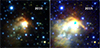 |
Fig. 1. VVV JHKs pre-burst (left) and burst (right) color composites (FoV 44″ × 44″, north is up and east is to the left). The central cyan-colored areas are due to detector saturation. |
The TIMMI2 image is shown in Fig. 2. The contours delineate [5, 35, 200, 560] × 1σ levels where the latter corresponds to half of the peak value. The lower-left circle shows the FWHM of a standard star measured before the object. Although the object was classified as point-like, the absence of the first Airy ring, expected for an unresolved source in diffraction-limited imaging, indicates that it is marginally resolved. By subtracting the FWHMs of the standard star in quadrature, a deconvolved size of  at a position angle of
  was obtained.
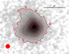 |
Fig. 2. TIMMI2 10.4 μm image (epoch 2006). The lower left circle shows the FWHM of a standard star measured before the object. The contours delineate [5, 35, 200, 560] × 1σ levels where the latter corresponds to half of the peak value. No Airy-rings are visible, although the source was classified as point-like. |
The appearance of the target in the various HAWC+ bands is shown in Fig. 3 where the image size is scaled to apparently “cancel” the wavelength dependence of the PSF. The absence of diffraction rings implies that the source is resolved at all HAWC+ wavelengths.
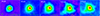 |
Fig. 3. HAWC+ log scaled image cutouts, centered on G323 and spatially scaled to the beam FWHM (lower left) for each band. The absence of Airy rings indicates that the source is resolved at all wavelengths. The horizontal line marks an angular size of 1′. |
3.2. IR light curves and color change
The IR light curves based on VVV(X) Ks-band as well as the (NEO)WISE photometry are shown in the left panel of Fig. 4. For comparison, the (NEO)WISE W1 and W2 light curves were shifted to match the pre-burst Ks-band magnitude. Since the (NEO)WISE fluxes in both bands exceed the limit for which a meaningful bias correction can be applied, the burst light curves are not suitable for drawing quantitative conclusions. However, they represent an independent confirmation of the event, heralded by a maser-flare. The integrated maser flux is plotted in green. The scatter during and after the burst is due to the short-term periodicity of 93.5 d (Proven-Adzri et al. 2019). The correlation between the maser flare and the burst is discussed in more detail in Sect. 3.4. The vertical red, and blue lines mark the dates of the burst onset, and the first flare evidence from the 6.035 GHz exOH maser (MacLeod et al. 2021).
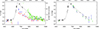 |
Fig. 4. Left: light curves based on VVV(X) (black) and (NEO)WISE photometry (W1 – blue, and W2 – red) as well as 6.7 GHz total maser flux (green, Green et al. 2015; MacLeod et al. 2021). Vertical red and blue lines mark the dates of the burst onset and first flare evidence from the 6.035 GHz exOH maser (MacLeod et al. 2021). The Ks rise was approximated by a polynomial, while its decay is roughly linear on a log scale (dashed line). The (NEO)WISE magnitudes are shifted to match those of Ks. The integrated maser flux is shown on a log scale (right ordinate). Its scatter is due to the short-term periodicity. Right: Ks (black), i (blue), and z (green) light curves, with i and z magnitudes shifted to match those of Ks. The z pre- and post-magnitudes agree within the errors. |
The temporal behavior of the Ks-band brightness can be subdivided into two phases. The burst appears to have started in early 2012, and we designate 5 June 2012 (MJD 56083) as its onset date. At that date, the polynomial rise approximation started to exceed the error margin of the mean pre-burst Ks-band magnitude of 7.91 mag. A particular rapid flux increase occurred in June 2013, probably shortly before the burst peak. The intersection of the polynomial rise approximation and the exponential decay of the NIR flux variability suggests that the peak date of the burst was in late summer 2013, probably around 31 August 2013 (MJD 56535). Then it fainted with a linear trend of 0.75 mag yr−1 which corresponds to a flux decline with an e-folding time of 3.3 yr. The pre-burst Ks magnitude was again reached around 27 September 2020 (MJD 59119). We consider this date to mark the end of the accretion burst, which then lasted ∼8.4 yr. The right panel of Fig. 4 shows the comparison of the i, and z-band light curve from the Skymapper survey with the Ks light curve. Both the i, and z bands confirm the end of the burst in 2020. The z post-burst magnitude is the same as the pre-burst magnitude within the given errors.
The color indices (H − Ks), and (J − H) were estimated from images in the J-, and H-band taken about 1.8 yr after the burst peak. They indicate that compared with its color during the pre-burst stage, the source was bluer by 0.7 mag in (H − Ks), and 0.62 mag in (J − H) at that time. Comparison of the W1, and W2 magnitudes at the burst peak appears to indicate that for G323 as well (see also Fig. 7). Young eruptive stars may become bluer or redder when brighter during the outburst (e.g., Lucas et al. 2024) which cannot be explained by variable extinction alone. For example, Contreras Peña et al. (2023) observed bluer (W1 − W2) burst colors in the embedded FUor SPICY 97 855.
3.3. The scattered light echo
In recent years, an increasing number of light echoes (LEs) from low-/intermediate-mass young stellar objects (YSOs) are identified (Ortiz et al. 2010; Hodapp & Chini 2015; Dahm & Hillenbrand 2017). The first observed LE associated with a MYSO burst is that of S255IR-NIRS3 (Caratti o Garatti et al. 2017; Stecklum et al. 2017). To assess the presence of a scattering LE of the G323 burst, optimal image subtraction (e.g., Alard & Lupton 1998) on the VVV(X) images was performed. For this purpose, the implementation using Interactive Data Language (IDL)8 was used (Miller et al. 2008). For each band, the pre-burst image with the smallest FWHM served as a reference. Spatial extinction variations across massive star-forming regions hamper LE detection in difference images. For this reason, ratio images were created by division with the reference image, which cancels these variations (assumed to be constant in time). This proved useful in revealing the LE of the S255IR-NIRS3 accretion burst (Caratti o Garatti et al. 2017).
An overview of the burst-induced change in the appearance of G323 is given by Fig. 5, showing the pre-burst, difference, and ratio images for the various VVV(X) filters. The difference and ratio images provide clear evidence of a light echo associated with G323. Another one 1 35 southeast of G323, which appeared later, can be seen in the sequence of Ks images (Fig. 6). We denote those as “prompt” and “remote” LEs. In the J, H, and Ks ratio images of Fig. 5, the highest values are not located close to the source, but at a distance that increases with wavelength. This illustrates the echo propagation and the dependence of its velocity on the optical depth, which is lower for longer wavelengths (e.g., Draine 2003).
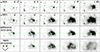 |
Fig. 5. Columns from left to right: Z, Y, J, H, and Ks images and rows from top to bottom: those of 2010, 2015, difference, and ratio (range 0…17.5). The crosshair marks the MYSO position. For the upper two rows, the values comprise 98 percentiles, displayed using a linear stretch. At red optical wavelengths (two leftmost columns), the object appears bipolar. Both blobs are probably due to scattering, with the eastern one brighter in Z. Both are offset from the nominal MYSO position and indicated by the red Z contours in Fig. 10. The prompt LE is visible in all five bands. Its large size in the Ks ratio image is due to a smaller number of scatterings compared to the other bands. A common foreground proper motion binary (blue arrow) appears in Z and J next to G323. The FoV amounts to 70″ × 45″. |
Light echoes (LEs) are also detected in the NEOWISE W1 and W2 images, which were retrieved using the ICORE tool (Masci 2013). This is not self-evident, as the scattering cross-section of interstellar dust grains at longer wavelengths is smaller (e.g., Draine 2003). However, the lower scattering efficiency is more than compensated by higher flux densities in the NEOWISE bands compared to Ks (cf. Fig. 15). The features of the LEs and their evolution seen by NEOWISE correspond to what is found in the Ks-band.
Near the source, the spatial brightness distribution of the LE echo represents a record of the burst history. Thus, the maximum of the ratio values provides an estimate of the maximum burst strength. This holds for the J- and H-bands, where the maximum values at various locations are around 20. Further away, the echo strength decreases as a result of spatial propagation and superposition along the line of sight. This is already the case for the Ks-band. Clearly, the LE is not circular-symmetric but extends southeast and is missing in the opposite direction. This indicates a nonuniform dust distribution in the environment of G323. The absence of an LE in the northwest could be related to the curved rim-shaped structure in this area (cf. Fig. 1) that could block or shadow it.
The temporal evolution of the source appearance during the burst can be seen in the sequence of Ks-band frames (Fig. 6), taken from 2010 to 2019. For illustrative purposes, images were selected with a time difference of about one year, except for a half year during the burst rise. Although this is only a subset of all Ks-band images, it nonetheless provides the most important information. To emphasize structural changes, the difference images are shown in Fig. 6. They can be traced on the ratio images as well, albeit at a lower dynamic range. Early signs of the burst are visible in 2012 which reached its full swing in the following year. The larger number of saturated pixels at the MYSO position indicates an increase in brightness. One year later (2014), the propagation of the prompt LE becomes obvious. An arc-like feature becomes visible that winds toward the east, as well as a straight one that is oriented toward the south. Until the next epoch (2015), the eastern arc-like feature vanished, and the straight one became arcuate with a strong turn. Over time, the burst light propagated into the interstellar medium, leading to the appearance of a remote LE in 2016, featuring variable illumination. The last frames of Fig. 6 also show the general fading of the source and its environment. Finally, an elliptical structure with the MYSO at its western apex is worth mentioning, as it is visible from 2015 to 2019. Due to its pertinent morphology, it has to be stationary. Perhaps this could be light scattered from the wall of an outflow cavity.
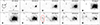 |
Fig. 6. Ks-band difference images showing the temporal evolution of the burst and the associated LEs, displayed using a log scale. The prompt echo, which originates from the cloud core, is monopolar and spreads to the southeast at an PA of ∼135°. A remote LE that appeared later traces denser structures of the ISM. The red polygon encloses the area from which its light curves were established. The FoV is 135″ × 80″. |
The remote LE is still faintly visible in NEOWISE images taken in 2023 (cf. Fig. A.1). Its light curves (Fig. 7) were established by integrating the fluxes in the Ks, W1, and W2 bands over this region, marked in Fig. 6. The subtracted background was derived from an area northwest of the MYSO, devoid of stars. Notably, these light curves cover the burst rise which is missing in the on-source data (cf. Fig. 4) because of the time gap between the WISE and NEOWISE missions. The primary characteristics that can be drawn from them are the following. The LE peak occurs slightly more than four years after the burst peak. Its amplitude is shallower than that of the burst, which is due to echo propagation. The W1 − W2 color change confirms the “bluening” during the burst. Due to the wavelength dependence of the scattering cross section, the pre-burst colors of the LE are bluer than those of the source, as indicated by Ks − W1 = 2.44 ± 0.20 vs. 3.20 ± 0.12 and W1 − W2 = 1.25 ± 0.23 vs. 1.56 ± 0.16.
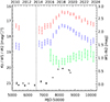 |
Fig. 7. Light curves of the remote LE where colored error bars denote the following: Ks (black), W1 (blue), W2 (red), and W1 − W2 color (green, right ordinate). The vertical dashed line marks the date of the burst peak. The LE peak occurs slightly more than four years after the burst peak. |
For common cases of LEs, as for example those associated with novae, supernovae, and variable stars (Sugerman 2007; Jiang et al. 2016; Kervella et al. 2008), a superluminal motion of the echo is present. It is a pure geometrical effect that follows from first principles in the case of single scattering (Nemiroff et al. 2016). Whether a prompt YSO LE is superluminal is questionable, since its environment is quite dusty. Thus, multiple scattering may overwhelm the geometric effect on which the superluminal motion rests. For G323, the apparent propagation velocity can be derived from the projected separation between the echo boundary and the MYSO, as well as the time difference between the date of the burst peak and the epoch of observation. For the Ks-band, the respective quantities are ∼22″ and one year. Together with a distance of 4.08 kpc, this yields 1.4 c. Although this confirms the superluminal motion in the Ks-band, it implies that the apparent velocity is smaller for H and J. Given the small extent of the J echo, its apparent velocity is probably close to subluminal.
In the optically thick regions, the photons follow random walk paths, where the effective travel distance is given by the diffusion path length. For random walk processes, the diffusion path length ldiff is  (assuming isotropic scattering), where lfree is the mean free path and nscat is the number of scattering events. Within a fixed time t the photons can travel a path with a “real” length of lreal = nscat ⋅ lfree ⋅ c, with c being the speed of light. The “real” path is the same for all wavelengths (it depends only on the travel time and c), but the interaction free path length (and hence the number of scattering events) depends on the optical depth (and hence the wavelength). When the equations are combined, the diffusion length at a given time and wavelength is ldiff(λ, t)∝lreal(t)⋅(nscat, λ)−1/2. This implies a difference in the diffusion path length (and hence the apparent LE extent) for different wavelengths. With nscat ∝ τ2 (see e.g., Krieger & Wolf 2021), the expected extent of the LE in Ks compared to that seen in Z can be written as the inverse ratio of the optical depths ldiff, Ks/ldiff, Z ∼ τZ/τKs. For MRN dust (Mathis et al. 1977), the optical depth ratio between the Z and Ks filters is τZ/τKs ∼ 3.8. This would imply that LE propagation is almost a factor four slower in Z than in Ks. However, the density within the cloud core is highly variable, and a measurable slowdown is expected only in the densest regions (close to the protostar) and therefore the effect will be smaller.
3.4. IR-maser correlation
Class II methanol masers are pumped by MIR radiation (e.g., Sobolev et al. 1997; Cragg et al. 2005). Therefore, variations in the pumping rate will change the maser flux. The recent accretion bursts from MYSOs were all accompanied by flares of those masers (e.g., Sugiyama et al. 2015, 2019; Hunter et al. 2017; Szymczak et al. 2018), which confirmed their radiative excitation. The correlation between mid-IR and maser radiation exists also for sources, that show periodic simultaneous maser and IR flares, such as G107.298+5.639 (Stecklum et al. 2018), G36.705+0.096 (Stecklum & Linz 2022), as well as G45.804−0.356, and G49.043−1.079 (Olech et al. 2022).
For the G323 burst, there is also a clear correlation between the maser flux and the Ks-band flux (cf. Fig. 4). We note that although NIR Ks-band photons do not pump the masers, the long-term variation of the integrated maser flux closely follows the Ks light curve, simply because the NIR and MIR maser-exciting radiation vary in the same fashion. A log–log regression yields a power-law exponent of 1.4 ± 0.12. Thus, the G323 burst strengthens the evidence that Class II methanol maser flares are a reliable tracer of episodic accretion variability of young massive stars.
An attempt to detect the maser periodicity in the VVV(X) photometry failed because the cadence of the NIR survey was insufficient. While (NEO)WISE is able to trace intraday variability during a visit for sources that are not too bright, the large photometric errors for saturated targets such as G323 precludes concluding whether its brightness varies in sync with the maser.
3.5. HAWC+ FIR photometry
As stated above, the main objective of the SOFIA/HAWC+ observations is to constrain the burst energy by assessing the strength of a possible FIR afterglow due to the burst. This was done by comparing the pre-burst fluxes from the HPPSC with those measured with HAWC+. Although the field sizes of the 53, 62, and 89 μm bands do not cover additional HPPSC sources, the larger fields of the 154 and 214 μm bands comprise one or more. The detection of the source HPPSC160A_J152920.2-562522 in the 154 μm image provides the opportunity to check the flux calibration. PSF photometry of this object revealed that its HAWC+ flux exceeds the PACS flux by (15 ± 7)%. Consequently, this was taken into account in the analysis. Furthermore, the HAWC+ 62 and 154 μm fluxes were interpolated to the PACS wavelengths using a polynomial approximation of the post-burst FIR SED established from all HAWC+ bands.
The flux growth curves with increasing aperture size are shown in Fig. 8 for the PACS 70 and 160 μm as well as for the HAWC+ counterparts. Red and blue mark the wavelengths, while dashed and solid lines indicate PACS and HAWC+ fluxes. The vertical lines point to aperture radii, which reproduce the HPPSC fluxes. The flux ratios HAWC+ vs. PACS for the blue and red bands were derived by dividing the values of the respective growth curves and taking their average. They amount to 1.142 ± 0.046 and 1.085 ± 0.061. The errors take into account the scatter of the growth-curve ratios and the relative uncertainties of the PACS fluxes as well as those of the HAWC+ calibration. The ratio values agree within their errors, which a posteriori confirms the 154 μm flux correction. They suggest the presence of a weak FIR flux excess, which stems from the burst afterglow.
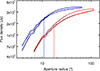 |
Fig. 8. Flux growth curves of PACS (dashed) and HAWC+ (solid). The wavelength bands are indicated by color, where blue is 62/70 and red 154/160 μm for HAWC+/PACS, respectively. The vertical lines mark the aperture radii, which reproduce the HPPSC fluxes. Black lines are polynomial approximations, reducing the influence of finite pixel size. The mean of the growth curve ratios gives the increase at the HAWC+ epoch. |
The HAWC+ fluxes were derived for all bands using aperture sizes tied to those obtained as outlined above using a linear relation for the wavelength dependence. The formal uncertainty obtained from the error images provided by the processing pipeline (DRP version 3.0.0) is in the range of a few Jansky only. The uncertainty of the flux calibration can be assessed from the residuals of a low-order polynomial fit to the observed fluxes, since the dust-continuum SED of the YSOs is continuous and featureless in the FIR (cf. Stecklum et al. 2021). This yields a relative error of 10%.
The HAWC+ photometry is given in Table A.1 along with beam sizes, as well as image and deconvolved FWHMs. The FWHMs of the image profile were derived by fitting an ellipse to the cut at 50% peak level. The uncertainty of the length of the axis ranges from 0 5 to 1
 5, while that of the position angles is ∼13°. The deconvolved sizes are based on the geometric mean of the major and minor axes, from which the beam size was subtracted in quadrature. The post-burst SED is plotted in Fig. 9 in orange (HAWC+ filters), with the interpolation to the PACS wavelengths in red. The pre-burst SED is shown in blue for comparison. The inset shows a zoom-in on the region of interest.
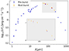 |
Fig. 9. Pre-burst SED (blue), together with the HAWC+ post-burst observations (orange). The HAWC+ observations were interpolated to match the wavelengths of the pre-burst observation. The resulting data points are colored red. The inset shows a zoom-in on the region of interest. The flux excess in the post-burst epoch is small (only ∼10% at 70, 160 μm). |
3.6. AO and thermal IR imagery
The pre-burst NACO Ks-band image is shown in Fig. 10. A logarithmic scale is used to display the lower surface brightness. The black diamond marks the peak position of 1.4 mm emission, based on the ALMAGAL data obtained with the ALMA 12-m array. This probably corresponds to the location of the MYSO. As mentioned in the caption of Fig. 5, the contours of the emission of the Z band are superimposed in red. The two scattering blobs are located southeast of the Ks-band peak. The western one coincides with the position of the Gaia source. The white contours delineate the 19 GHz radio continuum (Murphy et al. 2010), which is centered on the MYSO. The remaining symbols, filled circles with error bars, mark the positions of 6.7 GHz masers (blue – Caswell 1997, red – Green et al. 2015), as well as the width and orientation of the ISAAC slit (yellow). The tightly winded circular Z-band contours at the bottom are due to a foreground star that is barely visible at their center.
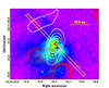 |
Fig. 10. NACO AO Ks-band image (epoch 2009) using a logarithmic stretch with contours of the 19 GHz radio continuum (white, Murphy et al. 2010) and from the Z-band pre-burst image (red, epoch 2010). Maser spots are marked by crosses in blue (Caswell & Reynolds 2001, epoch 1994) and red (Green et al. 2015, epoch 2011), with sizes indicating the position error. The black diamond is at the peak of the 1.4 mm emission while the black square marks the Gaia source. The yellow rectangle shows orientation and width of the ISAAC slit. |
The field stars in the NACO AO image have FWHMs of the order of 0 11–0
11–0 16. Therefore, the image can be well compared with the available radio data of similar resolution and position accuracy. It provides information on linear spatial scales of about 500 au. The elliptical image core is marginally resolved. The FWHMs obtained by a bivariate Gaussian fit are 0
 254 and 0
 177, and the major axis is at a position angle (PA) of 28
 5. This corresponds to the beam-deconvolved linear sizes of 890 au and 490 au, respectively. The ISAAC slit (PA = 43
 8) applied for K band spectroscopy is almost aligned with the major axis. Both PAs are not too far from those of the HAWC+ images listed in Table A.1.
3.7. K-band spectroscopy
The spectral image shows a rising continuum and two bright emission lines, namely the H I Brγ line at 2.166 μm and the H2 1–0 S(1) line at 2.122 μm. A zoom-in on the continuum-subtracted spectral image is given in Fig. 11. There may be a third line, well below the 3σ detection, centered around ∼2.206 μm. If real, this line would be one of the two Na I doublet lines often detected in the K-band (Caratti o Garatti et al. 2017), the second one (at 2.208 μm) falls beyond our spectral coverage. In fact, the spectral image covers a small portion of the K band. Therefore, other important features, such as the CO band heads (between 2.28 and 2.5 μm) that trace disk-mediated accretion are not included.
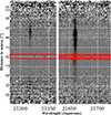 |
Fig. 11. Zoom-in sections of the continuum-subtracted spectral image showing 2.122 μm H2 (left) and 2.166 μm Brγ (right), both featuring extended emission. Red contours show the source continuum emission (1 − 3) × 10−14 erg s−1 cm−2 Å−1. NE is up. |
Both the continuum and detected lines extend a few arc seconds farther away from the point source position and are probably scattered along the outflow cavities. While the Brγ line extends toward NE and SW along the slit, the H2 emission is detected toward NE and is not seen at the source or toward SW (see Fig. 11). There may be a faint H2 emission toward the SW, but it is well below the 3σ detection limit.
Table 1 lists line fluxes, full width at half maximum (FWHM), peak radial velocities (vr) and full width at zero intensity (FWZI) of Brγ and H2 along the three different regions extracted from the spectral image, namely at the source, toward the NE and SW of the source. The H2 emission, only detected in the NE region, is spectrally unresolved (FWHM ∼ 2.4 Å or 34 km s−1) and its maximum radial velocity is around 0 km s−1 or slightly redshifted (4 ± 4 km s−1). The H2 kinematics points to fluorescent emission from the HCHII region around the source. On the other hand, the kinematics of the Brγ line is more complex. The line is spectrally resolved in the three extracted regions. It has a radial velocity close to 0 km s−1 on source, whereas the SW region is slightly blueshifted (–14 ± 5 km s−1) whereas the NE region has three different velocity components at –28, 2, and 32 km s−1. Furthermore, the FWZI values of the line in the three regions range from 150 to 170 km s−1. Spectroscopy was performed during the light-curve rise, close to the NIR peak of the outburst. At that time, no P-Cygni profile was present in the Brγ line. This feature is commonly attributed to an emerging ionized wind. Its absence in the G323 spectrum may indicate that the launching of the wind is not a prompt process, but delayed with respect to the temporal evolution of the burst. This was observed for the S255IR-NIRS3 outburst (Cesaroni et al. 2018).
Fluxes and kinematics of the Brγ and H2 (2.12 μm) lines.
3.8. The ALMA view of G323
The ALMA continuum and line data are a crucial supplement for the IR observations to complete the characterization of the MYSO. We emphasize that the data were taken at the end of 2019, less than one year before the burst end. Figure 12 shows the 1.4 mm dust continuum map taken with an 80th percent baseline length (L80BL) of 511 m which indicates that the source is resolved by a few beams. The contours start at 5σ (σ = 1.6 mJy beam−1) and increase in steps of 20σ. At the lowest level, it is not circular but shows extended emission.
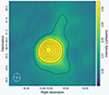 |
Fig. 12. 1.4 mm dust continuum map with superimposed contours. The ellipse on the lower left indicates the beam size. The object is resolved and shows faint extended emission. |
Figure 13 displays the first moment of SiO line emission along with the contours of the dust continuum at a coarser resolution, based on observations with an L80BL value of 126 m. The line emission is centered on the millimeter source and shows a velocity gradient from the SE to the NW. This indicates that the gas to the SE is redshifted. The velocity interval is rather small for the source being seen face-on, which argues against an origin of the emission in an outflow. There is no sign of Keplerian rotation for which the largest velocity differences would be at the center. The coarse resolution of the ALMA 12-m array is not sufficient to resolve a possible disk.
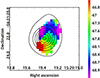 |
Fig. 13. First moment of the SiO emission with superimposed dust continuum contours from the ALMA 12-m array. The color bar indicates the velocity interval, in units of km s−1. There is a slight gradient from the SE to the NW. |
The contours of the intensity map of the blueshifted and redshifted 13CO(2–1) emission are shown in Fig. 14, superimposed on a Ks image taken in mid-2015 along with the 1.4 mm continuum emission. The latter appears as a small blob in the white area of the saturated central region. The synthesized beam size ( ) of the 13CO(2–1) observations is shown on the bottom left. The line emission was integrated in the LSR velocity ranges from 7 to 18 km s−1 for the redshifted gas and from –7 to –15 km s−1 for the blueshifted gas. The contours begin at 5σ and increase in steps of 2σ where σ is 0.18 Jy beam−1 km s−1 and 0.13 Jy beam−1 km s−1 for the redshifted and blueshifted lobes, respectively. Remarkably, the blueshifted gas appears to coincide with the dusty ridge west of the MYSO while the redshifted emission toward the east is co-spatial with the NIR nebulosity. This is not typical for outflow cavities, which are usually devoid of dust and scatter from their walls. If the CO emission traces an outflow of a source seen almost pole-on, its bipolar lobes should overlap more strongly than is the case for G323. Moreover, considerable bending seems to be present. Although this challenges the outflow interpretation and possibly argues for bulk-gas motion, a deflection of the blueshifted lobe at the western dust rim cannot be ruled out. Unfortunately, the ALMA 1.4 mm map is not sufficiently sensitive to shed light on the dust distribution at larger scales. Inspection of the SPITZER/IRAC images does not provide evidence for a bipolar outflow as well. Unlike other MYSOs, for which outflows were found (e.g., Caratti o Garatti et al. 2015), the IRAC2 image, which covers a wealth of shock-excited H2 lines (e.g., Noriega-Crespo et al. 2004), does not show typical bow-like emission features on either side of the source.
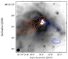 |
Fig. 14. Distribution of the redshifted and blueshifted 13CO (2–1) line emission as mapped with the ALMA 12-m Array superimposed on a Ks image taken in mid-2015. The synthesized ALMA beam size for the line observations is shown in the lower left. The compact 1.4 mm emission, mapped at much higher resolution, appears as a small blob within the white saturated pixels. |
4. Radiative transfer modeling
4.1. The static pre-burst model
In order to obtain a first guess pre-burst model, we chose a similar approach as introduced in Robitaille (2017), where a pool of SEDs is generated for a sample of different YSO configurations, that consist of the same set of components. For this purpose, we applied the TORUS code (Harries et al. 2019) its radiative equilibrium mode to generate a database of pre-burst SEDs. This is the same code used for time-dependent modeling as well.
We assumed an axisymmetric geometry, and the state variables (temperature, density etc.) were stored as a 2-D cylindrical adaptive mesh. The code employs Monte Carlo (MC) radiative transfer (MCRT), splitting the radiation field into a large number of indivisible photon packets that propagate through the mesh. An iterative method is used to determine the dust temperature based on the radiative-equilibrium method of Lucy (1999) and described in detail in Harries et al. (2019). Once the temperature distribution has been determined a second MCRT calculation is used to produce the SED at the given inclination.
All models are composed of a protostar, a passive disk, a curved bipolar cavity, and an Ulrich-type envelope (Ulrich 1976). The disk can be described as a flared disk in hydrostatic equilibrium (Chiang & Goldreich 1997), but, similar to Robitaille (2017), the parameter ranges are chosen such that flat disks are included as well. The passive disk approach is justified for FIR/(sub)mm wavelength regions. Active disks (e.g., Shakura & Sunyaev 1973) differ from passive disks mainly in the innermost region, where most of the energy is released by viscous dissipation (Pringle 1981). Thus, the difference manifests primarily in the MIR, which might rise earlier in the case of active disks and maybe even before the source and/or NIR peak. To model the thermal FIR afterglow, the passive disk approach can be applied.
We used MRN dust (Mathis et al. 1977), which consists of compact, homogeneous, and spherical grains with a composition of 62.5% silicate and 37.5% graphite, where we took the optical properties from Weingartner & Draine (2001). The size distribution can be described by a power law with n ∝ a−3.5 with grain sizes ranging from amin = 5 nm to amax = 250 nm. All parameters were sampled from the ranges given in Table 2. The protostellar luminosity L* includes all possible mechanisms of energy release (fusion, contraction, accretion). Throughout the paper the term “luminosity” represents the bolometric one, obtained by integrating the SED over the whole wavelength range observed. The inner radius of the circumstellar disk is governed by the dust sublimation radius (assuming Tsub = 1600 K). For our models, we cut the envelope at an outer radius renv, which was sampled between (1 − 4)×104 au (0.05 − 0.2 pc). This is in the range of the size of a typical cloud core. The extent of the FWHM in the ALMA images is smaller by a factor of two to ten. Due to the high resolution, the interferometer may not be sensitive to the extended component of the emission. However, most of the emission should be covered by ALMA. The extent of the prompt LE is greater than the outer radius of our models by a factor of ∼5. However, the density in the outermost parts of the parent cloud core is probably pretty low.
Adapted parameter spaces and sampling for the TORUS pre-burst models.
In total, we include 2500 SEDs. Although this seems small compared to the YSO grid of Robitaille (2017), we applied a much smaller range of protostellar luminosities. Therefore, the density of models in the parameter space is actually similar. Figure 15 shows the pre-burst SED (blue) together with the model pool (gray). The data is reproduced pretty well. The spikes visible in the MIR are due to low photon counts. To save computing time, we initially used only a relatively small number of photon packets for the models. Models that provide good fits were recalculated with a sufficient number. The pre-models were fitted assuming a distance of  kpc and a foreground extinction of AV = (18 ± 1) mag as given in Sect. 1.
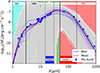 |
Fig. 15. All TORUS models (gray), together with the pre-burst SED (blue dots), the ten best fits (blue, the best one is darkest), and the mean model (red). The model SEDs are reddened according to the foreground extinction of 18 mag (Murphy et al. 2010). Background colors indicate different wavelength ranges. The SED peaks in the MIR/FIR. The wavelength range of HAWC+ is indicated at the bottom. That for radiative maser excitation (Ostrovskii & Sobolev 2002) is highlighted in blue. Flux densities are listed in Table A.3. The mean model fits the pre-burst SED quite well. |
The G323 pre-burst SED is well covered from NIR to (sub)mm. The number of free parameters is as large as 11 and there are degeneracies among the models. Therefore, we do not use just the best model, but rely on the ten best models instead. This approach was applied already in Stecklum et al. (2021). All parameters of the ten best pre-burst models (blue) are averaged using weights according to the respective χ2 value. For linear sampled parameters, we use the arithmetic mean, whereas for logarithmically sampled parameters, it is the geometric mean. The resulting mean model, that is, the model where all parameters are mean values, is colored red. The mean values can be found in the right column of Table 2. The table with the ten best models is given in Table A.6.
Note that the best models point to an almost face-on view. The inclination is smaller than the opening angle of the cavity, which implies that the optical depth toward the object is minimized.
In addition to the mean model, two additional settings are included (Tmin and Tmax). These settings minimize and maximize the afterglow timescales and compromise parameters, which are in agreement with the pre-burst fit within the given confidence intervals. The Tmin setting has a lower dust content, and a wider opening angle of the cavity compared to the mean setting. The Tmax setting has a higher dust content, and a smaller cavity opening angle. The parameters of all three models are summarized in Table 3, where only those that differ are given. We changed only those parameters that are considered to strongly affect the duration of the afterglow. All other parameters are the same as for the mean model (right column of Table 2). Constant parameters are the protostellar luminosity, inclination, and most of the disk parameters, since their impact is small or unclear. The Tmin, and Tmax settings are meant to give limits on the burst energy that take into account that the afterglow depends not only on the burst energy but also on the local dust distribution. Both the mean, and the Tmax models agree well with the pre-burst SED (their χ2 is comparable or better than that of the best-fit model). The Tmin model has too little cold dust and cannot reproduce the FIR fluxes. However, TDRT models were also performed for this model.
Overview over the simulation settings.
4.2. TDRT modeling
4.2.1. TORUS-Code
To model the temporal evolution of the SED, the TORUS radiative transfer code was used in its time-dependent mode. The time-dependent algorithm follows the random walk of photon packets as they propagate over a time step, with the energy absorption rates for each grid cell calculated using a MC estimator and the energy emission rate calculated from the local dust temperature. The TDRT method is described in detail in Harries (2011) and has been benchmarked against several standard thermodynamic test problems. Unlike traditional methods, such as flux-limited diffusion, the code is able to simultaneously and accurately treat both the free-streaming and diffusive regimes. The role of the time step is crucial to the accuracy of the calculation. It needs to be short enough for the luminosity variation to remain tractable, but long enough to avoid creating too much computational overhead (Harries et al. 2019). We used a time step of 3.65 d, which was verified with an interval shorter by a factor ∼7. With this choice, the envelope heating, which is responsible for most of the FIR radiation, is traced very well. But for the disk, a shorter time step is better. TORUS is a very versatile code with several microphysics modules from which we only apply those to calculate the dust radiative equilibrium (static RT) and nonequilibrium (TDRT). The former was used, for example by Esau et al. (2014) while the latter was validated against the Pascucci disk benchmark (Pascucci et al. 2004).
4.2.2. Assumptions and constraints
To derive the burst energy using TDRT, we make several assumptions, which are explained below. TORUS computes dust continuum emission as a function of time and wavelength for a given source-luminosity variation and local dust distribution.
First, we examine whether the energy radiated away by dust is a good proxy for the total energy released by the burst. The two main coolants for YSOs are molecular lines, in particular from CO, and dust radiation. Dust grains are solids, which implies that they are thermal emitters. Their opacities cover more than four orders of magnitude in wavelength of the electromagnetic spectrum (e.g., Min 2015) and are thus much more capable of affecting radiative heat transfer than gas opacities. In fact, the luminosity of the FIR molecular cooling lines of MYSOs is only a tiny fraction (∼10−5, Karska et al. 2014) of the dust luminosity. The same holds for the energy release by free–free emission from a compact HII region (Cesaroni, R., priv. comm.). Therefore, the luminosity estimate derived from the SED can be considered as the total value.
Although the gas cooling is not relevant for the energy considerations, we note in passing that the heating/cooling timescales for dust and gas may differ. At volumetric densities ≳1.2 × 104 cm−3 (e.g., Merello et al. 2019) gas and dust are thermally coupled through collisions. In the (dense) innermost regions of MYSOs this assumption is certainly justified. In the extended outer envelope the coupling may be weaker. Then, the gas will heat/cool much slower than the dust (see, e.g., Johnstone et al. 2013). Therefore, the response of the gas cooling lines to an accretion burst may be strongly delayed in comparison to that predicted by our TDRT model.
The dust distribution is given by our three reference models: Tmin, mean, and Tmax (as introduced in Sect. 4.1). We assume that the Ks light curve may serve as a proxy for the variation of the accretion rate, which is hereafter referred to as the “burst profile”. It is essentially defined by the dates of the burst rise, its peak, and the return to the pre-burst Ks level. According to Wien’s law, the effective wavelength of this band is closest to the dust sublimation temperature. Even with the recent Skymapper release, the VVV(X) Ks photometry still provides the best coverage of the burst evolution. Moreover, this choice is justified by the almost face-on view of the best-fitting pre-burst models (see Sect. 4.1), allowing for a “direct look” at the innermost regions, where the VIS/NIR-photons originate.
For TDRT modeling, we use the most simple approach possible, namely, we include only heating and cooling but omit any kind of density variation as well as any changes in the disk chemistry. The latter is generally not met. Instead, the burst will most likely sublimate the innermost disk, change the chemistry of the disk, and shift the ice line outward (e.g., Lee 2007; Visser & Bergin 2012; Vorobyov et al. 2013; Rab et al. 2017). In principle, dust sublimation is implemented in TORUS but it requires a time step of less than 1 d to remove the disk on typical disk dispersal timescales. However, the impact on the evolution of the (F)IR luminosity will be minor. Therefore, we use a longer time step, where we move the inner radius outward to ensure that the dust does not become hotter than Tsub. We shift it to 60 au, which is ∼3 Rsub according to Whitney et al. (2004, Eq. (1), with Tsub = 1600 K), where we kept the disk mass constant.
4.3. The dynamic SED of the mean model
This is the first astrophysical application of dust-continuum TDRT. Therefore, we briefly discuss one particular model in more detail before fitting the burst energy. We used the mean model with an outburst energy of Eacc = 2.3 × 1047 erg. This first guess for the burst energy is based on the assumption that the increase in Ks is the same as the increase in luminosity at all times. With the model setup and the burst profile at hand, TDRT simulations were performed. The result is shown in Fig. 16. The figure displays the dynamic SED, which is the flux density over wavelength and time. This probably provides the most concise overview of the entire afterglow. Time increases from top to bottom, where zero corresponds to the burst onset. Three particular times are indicated: Flux peak time (tpeak, white triangles), the time when 80% of the energy is released (t80, black dots), and the time when the flux density dropped to 1.25 times of its pre-burst value (t25, gray crosses) for each wavelength.
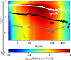 |
Fig. 16. Dynamic SED showing the flux density over wavelength and time (increasing from top to bottom) of the mean-setting and a burst with an energy of 2.3 × 1047 erg. Time 0 marks the onset of the burst. Horizontal lines indicate the peak time (white triangles), the time when 80% of the energy is released in the respective band (black dots), and when the flux increase is back at 1.25 times the pre-burst level (gray crosses). The increase in scatter in the (sub)mm range is due to lower synthetic photon counts. |
Both tpeak and t80 increase with wavelength. This is expected since the radiation at longer wavelengths can be attributed to regions more distant from the star (i.e., colder regions). Interestingly, the delay between NIR and FIR is almost two (and three) years for tpeak (and t80) at 100 μm. For comparison, the light travel time from the source to the outer edge of the grid is only 160 d. The delay between the peak of the burst profile (1.2 yr after onset) and that in the FIR is by far more than what could be explained by geometrical/projection effects and distinct spatial origins alone. It clearly indicates a measurable slowdown of the energy transfer toward the FIR-emitting regions by numerous absorption and re-emission processes owing to the high optical depths in between the protostar and FIR-emitting regions. Toward longer wavelengths (λ ≥ 300 μm) both curves flatten. This is expected because at some point even the coldest and most distant regions are “processed” and we are reaching the Rayleigh–Jeans tail of the emission from the coldest dust with ∼20K. Furthermore, these regions are generally optically thin at these wavelengths.
The t25-curve looks somewhat different. The time increases only slightly; it is almost constant between 30 and 80 μm and decays for λ exceeding 100 μm. Although the timescales increase in principle with wavelength, the peak level is much lower at higher wavelengths (at some point hindering a further increase of t25). At 4 to 8 μm there is a “prominent” feature and a weaker one at ∼15 μm. These MIR features can most likely be attributed to the densest regions (disk midplane), which cannot efficiently cool because of the high optical depths in the silicate absorption bands. For weaker bursts or less dense environments, this will probably not occur since the disk will not completely heat or cooling is faster. However, this requires further investigation. Toward long wavelengths, the synthetic noise increases dramatically because of the low number of photon packets. We emphasize that t80 is the timescale least sensitive to numerical scatter.
4.4. Results of the time-dependent fitting
4.4.1. Burst energy estimate for the mean model
In general, the reprocessed FIR radiation provides an indirect but reliable measure of the burst energy, since it covers most of the emission (SED peak) and the role of extinction is rather small (compared to the NIR/MIR), while the maximum increase due to the burst is still strong (contrary to the (sub)mm). FIR measurements were used successfully to estimate the energy of MYSO bursts in the past (Caratti o Garatti et al. 2017; Stecklum et al. 2021). For a more general discussion of the power of FIR data, based on static RT for a sample of low-mass YSOs, see, for example, Fischer et al. (2024).
In the following, we use the SOFIA post-burst FIR measurements together with a set of time-dependent models to constrain the burst energy. Our HAWC+ measurements indicate that the post-burst flux densities are slightly higher than the pre-burst ones. They are elevated by (14.2 ± 4.6)% at 70 μm and (8.5 ± 6.1)% at 160 μm (see Sect. 3.5). As the excess is quite small, we fit the flux density ratios rather than the absolute values. The ratios trace the increase in the protostellar luminosity and hence the released energy.
To constrain the burst energy, we performed seven simulations with burst energies between (0.2 and 7)×1047 erg. The corresponding burst templates (simulation input) are displayed in the left panel of Fig. 17 with the different burst profiles color-coded. The middle and right panels show the corresponding flux density ratios over time for 70, and 160 μm respectively. As the dust distribution is the same in all cases, the changes are due to the different energy inputs of the respective bursts. Obviously, the more energetic the burst, the longer the afterglow. Zoom-in to the HAWC+ data (red points in the inset) shows that the observed excess can be explained by a burst within the adapted energy range. The simulations (colored dots) show a lot of scatter. Therefore, we apply a stepwise interpolation in time (solid lines with confidence intervals in transparent).
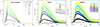 |
Fig. 17. Input burst profiles (left) and output flux ratios as a function of time for 70 (middle) and 160 μm (right) for the mean model. The burst energy is varied between (0.23 and 6.9)×1047 erg (color-coded). Obviously, the afterglows are longer for more energetic bursts. The geometry is the same for all simulations. The HAWC+ measurements are colored red. The horizontal solid and dashed-dotted lines mark the pre-burst level and 1.25 times that level. The insets show a zoom-in on the region of interest. The simulations (colored dots) were interpolated in time to reduce numerical scatter (corresponding lines and shaded regions). The observations are given in red. |
The predicted flux ratios at the date of the HAWC+ observation are shown in Fig. 18 as functions of the burst energy for 70 (blue), and 160 μm (red). The errors correspond to the confidence interval of the interpolation in time (at the HAWC+ date) for each model and wavelength (cf. the inset in Fig. 17). The HAWC+/PACS ratios are indicated by the dashed horizontal lines with the corresponding 1σ confidence intervals indicated by the colored areas. The ratios can be fitted with linear functions in the given range (indicated by the colored solid lines), whereby the y-axis intercept equals one, as no energy input means no flux increase. The fit leads to r70 = 0.06 ⋅ Eacc + 1 and r160 = 0.04 ⋅ Eacc + 1 with r70 and r160 as ratios at 70 and 160 μm respectively, and Eacc as the burst energy. A χ2 minimization yields a burst energy of Eacc = (2.4 ± 1.0) × 1047 erg (gray-shaded area with vertical black lines). The error ranges extend until the χ2 value becomes worse than  (the 1σ confidence interval according to kafe9).
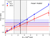 |
Fig. 18. Modeled flux ratio at 70 (blue) and 160 μm (red dots) for different burst energies, all featuring the mean setting. Solid lines are linear fits. The dashed horizontal lines are the observations with confidence intervals (overlapping colored areas). The vertical black line indicates the best burst energy Eacc for both wavelengths. The 1σ-confidence interval is indicated. We use a χ2-minimization to determine Eacc, where we use linear fits (colored solid lines) as model values for both wavelengths. We take into account the observational errors and uncertainties of the modeled ratios, where the contribution of the latter is minor. |
4.4.2. Limits on the burst energy
In the previous section we estimate the burst energy by using the mean model. Although the result agrees very well with our initial estimate, to assess its credibility, it is necessary to investigate the influence of the local dust distribution.
To show that the afterglow durations can be quite different we plot the dynamic SEDs for two different YSO configurations in Fig. 19. The left panel shows the dynamic SEDs for the Tmin and the right panel shows the Tmax setting. Both settings feature the same burst and the huge differences can be explained solely by the different YSO configurations. We emphasize that the Tmin and Tmax settings are limiting cases with minimal and maximal afterglow durations, respectively. This implies that the energy needed to explain the HAWC+ measurements can be considerably larger or smaller than that of our previous mean model estimate.
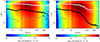 |
Fig. 19. Same as Fig. 16 but for the Tmin (left) and Tmax (right) setting. The burst is the same for both. The plot shows that the dust distribution strongly imprints the afterglow. For denser and more extended envelopes, the MIR/FIR afterglow can be significantly longer. Horizontal lines indicate the times when the peak is reached (white triangles), when 80% of the energy is released (black dots), and the time when the flux density is back at 1.25 × Lpre(λ) (gray). |
To determine the limits for the burst energy, we repeat the analysis from Sect. 4.4.1. We ran seven simulations for the Tmin setting with burst energies between (2.3 and 28)×1047 erg and nine simulations for the Tmax setting with burst energies between (0.05 and 2.3)×1047 erg. The ratios on the HAWC+ dates are shown in Fig. 20 for Tmin (top) and Tmax (bottom), respectively. A linear fit leads to r70 = 0.24 ⋅ Eacc + 1 and r160 = 0.35 ⋅ Eacc + 1 for Tmax and r70 = 0.005 ⋅ Eacc + 1 and r160 = 0.003 ⋅ Eacc + 1 for Tmin with r70 and r160 as ratios at 70 and 160 μm respectively and Eacc as burst energy. For the Tmax setting, the ratio at 160 μm exceeds the one at 70 μm. This is in agreement with the dynamic SED (Fig. 19), which shows a strong increase of the indicated timescales in between ∼(50 and 300) μm. Again, the best estimate for the burst energy is indicated by vertical lines. It amounts to 30 ± 12 for Tmin and  for Tmax in units of 1047 erg. For the Tmin and Tmax settings, the values of Eacc are about a factor 13 above and a factor six below the mean model respectively. We emphasize that the higher value is not likely, as the pre-burst fit of this model is much worse than for the other two settings. However, it may still serve as a conservative upper limit. A summary of the derived burst parameters is provided in Table 4.
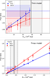 |
Fig. 20. Same as Fig. 18, but for the Tmin and Tmax model (top and bottom, respectively). For these settings, the burst energy (indicated by the vertical black line) needed to explain the HAWC+ data (horizontal red and blue lines) is maximized or minimized respectively. Interestingly, for the Tmax setting, which is the most extended and densest, the flux ratio at 160 μm (red) exceeds that at 70 μm (blue). The dependency is almost linear. The best fits are indicated by the solid colored lines. Note the different scales. |
Summary of the burst parameters for all three settings.
In addition to the HAWC+ flux density ratios, the models can be compared with the Ks measurements. Similar to the HAWC+ fit, we used the Ks flux density ratios. Figure 21 shows the Ks ratio curves for all three configurations (from left to right) and all burst energies (color-coded). The observation is shown in red. For the Tmin configuration and the highest burst energies, the Ks flux does not return to its pre-burst level at the end of the burst. This is probably caused by dust that becomes hotter than Tsub. We shifted the innermost radius to 60 au (∼3 Rsub) to avoid too high dust temperatures for all models. This is not sufficient for the most energetic bursts. All bursts overestimate the observed Ks ratio (red) for the Tmin setting. This is another indication that the burst energy estimate obtained with this setting is too large. We emphasize that the Ks ratio depends only slightly on the setting. For nearly the same burst energy for Tmin and the mean setting, the best match is reached with the Ks curve, despite the vastly different afterglows. Therefore, the Ks ratio provides a good measure for the burst energy. For both the mean and the Tmax setting, a good agreement is reached for a burst with an energy of 0.93 × 1047 erg. This value lies well within the determined range and would imply a dust configuration in the range between mean and Tmax. Probably the best estimate of the burst energy is  , which is based on the Ks value and covers the entire range spanned by the mean and Tmax settings. This would correspond to a peak value of
  , and hence an increase of the luminosity of the protostar by a factor
  (or ΔL ∼ 2.6 × 10⁵ L⊙).
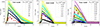 |
Fig. 21. Modeled Ks ratio curve for the Tmin (left), mean (middle), and Tmax (right) model setups featuring different bursts (in 1047 erg, color-coded). The observed Ks increase is shown in red for comparison. The ratio depends more on the energy input than on the setting. The best agreement is reached for Eacc = 0.93 × 1047 erg. For the Tmin setting and the highest burst energies, the Ks curves decay delayed, this might be an artifact due to the innermost dust becoming unrealistically hot (rmin is fixed to 60 au, that is, 3 × Rsub). We note that the ordinate scales are different. |
4.4.3. Accreted mass and mass accretion rate
From the burst energy, the accreted mass can be inferred with  . where G is the gravitational constant and R* and M* are the protostellar radius and mass. This approach is used for a passive disk in Stecklum et al. (2021). The underlying assumption is that the infalling material falls from a large distance onto the protostellar surface, where it releases its entire gravitational energy within the burst.
Although the SED shape, the NIR brightness, and the presence of an HCHII suggest that G323 is a more evolved MYSO, it must be kept in mind that its spectral appearance is dominated by the face-on view. Nevertheless, assuming that it is on the ZAMS will provide a lower limit of the accreted mass as protostars contract toward this locus of stellar evolution. For a star with a luminosity of  , the ZAMS mass amounts to
  and the corresponding radius
  (Tout et al. 1996, Eqs. (1) and (2)). The resulting parameters are summarized in Table 4. Adopting these parameter values, an accreted mass between 1.4 and 30 Jupiter masses (or 450 and 9 000 Earth masses) is derived. The errors are dominated by the uncertainty on Eacc.
With the accreted mass at hand, the average mass accretion rate ⟨Ṁacc⟩ = M/Δt follows as  , where Δt is the burst duration of 8.4 yr. For comparison, an upper limit of the quiescence accretion rate is given by
  , assuming that the entire pre-burst luminosity is due to accretion. Inserting the values yields 5.4 × 10⁻⁴ M⊙ yr−1.
5. Discussion
5.1. Accretion burst evidence
The Ks and (NEO)WISE light curves, together with the maser measurements, provided clear evidence of the previous accretion burst. Although discovered later, it actually started about three years before the discovery of the S255IR-NIRS3 (Caratti o Garatti et al. 2017) and NGC 6334I MM1 (Hunter et al. 2017) events in 2015. This is another example of a disk-mediated accretion outburst. We emphasize the fact that, thanks to the almost face-on view, the Ks light curve of G323 is the most direct trace of accretion variability during a MYSO burst obtained so far. Although the burst of S255IR-NIRS3 was also photometrically monitored in the Ks-band (Uchiyama et al. 2020), its emergent light curve suffered from multiple scattering due to the close to edge-on view. Thus, the case of G323 will be crucial for comparing accretion burst models with real events. Progress in this direction is ongoing (see, e.g., Elbakyan et al. 2023).
5.2. Reliability of the derived burst energy
Since the burst energy is crucial for understanding the burst physics, restrictions of our approach and how they can be overcome will be addressed in the following. The estimated range for the accretion energy of the G323 burst is fairly large (Sect. 4.4.2). We use only three settings, which are meant to provide limits. In principle, the best method to quantitatively analyze the afterglow requires a preferably huge set of different settings, which are all capable of reproducing the pre-burst SED (see Sect. 5.6). This is planned for the near future and is expected to lead to refined values.
In our analysis, we did not consider different burst shapes, but only varied the burst energy. This is justified by the availability of the Ks light curve which is a good proxy for the temporal variation of Ṁacc as confirmed by our modeling, cf. Sect. 4.4.2. Further support of this choice comes from the i and z-band measurements that show the same qualitative behavior.
The burst energy estimate was obtained using two approaches: we compared the HAWC+ post-burst flux density ratios and the Ks ratio curve individually (for all three settings). The results agree pretty well, which strengthens our approach. Our final estimate of the burst energy is based on the fit to the Ks ratio curve, while the confidence intervals are based on the HAWC+ fits.
In the following, we discuss how well the Ks flux increase is reproduced by our models. We neglect all the changes that may occur during the burst. But this will not be the case in reality. The most obvious change is probably the shift of the sublimation radius due to the burst. To investigate the effect, we performed a simulation that includes dust sublimation. We set the innermost radius at Rsub (20 au) and chose a time step of 0.7 days. Dust with a temperature greater than 1600 K was removed at each time step. The Ks radiation is produced by the hottest dust. Therefore, we cut the grid at the outer edge of the disk. With this choice, the resolution in the innermost regions is higher, while the entire Ks flux is captured. The result is plotted in Fig. 22. The maximum Ks ratio is about a factor of 1.5 smaller for the more realistic sublimation model (blue) compared to the mean model (black). The burst energy (and shape) are the same in both cases. This result might be surprising, as the emitting surface area should increase as the inner rim moves outward. Therefore, the ratio should be higher when dust sublimation is included. However, the inner radius of the mean model was set at 3 Rsub to avoid unrealistic high temperatures. Thus, the area where the Ks-band photons are emitted is larger. This shows that the most probable value (for Eacc) is slightly higher than our estimate, which does neglect dust sublimation. One could argue that a small fraction of the burst energy is needed to sublimate the disk, which might compensate for the above effect. However, this fraction is probably negligible. Typical values for the sublimation enthalpy range from 1 (hydrogen) to almost 1000 kJ mol−1 (graphite). With a molar mass of 2 g mol−1 (H2) and a gas-to-dust ratio of 100, it would take less than 1044 erg to sublimate 1 M⊙ (on the order of a total disk mass or more). This is less than 1% of the burst energy.
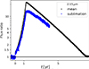 |
Fig. 22. Predicted Ks ratio for the mean model with (blue) and without (black) dust sublimation. Without dust sublimation, the increase is overpredicted by a factor of ∼1.5. |
Another issue that could impact the visible NIR flux is line-of-sight extinction variations. As the extinction is highly wavelength dependent, small changes may be enough to alter the Ks-magnitude. Tidal disruption or evaporation of the accreted object may increase the extinction, while on the opposite FUor/EXor outbursts are often accompanied by winds, which will blow out dust grains and thus reduce it (see, e.g., Reipurth & Aspin 2004; Mosoni et al. 2013). However, the Ks light curve does not show hints of sudden extinction changes. This is confirmed by the i and z-band flux densities, which are the same within the errors after and before the burst.
The cooling efficiency depends not only on the local temperature but also on the grain size and material. We use a mixture of amorphous silicate (astronomical silicate, astrosil) and carbon with small grains (MRN dust; Mathis et al. 1977), which are efficient in cooling. However, especially within the disk and also within the envelope, grain growth processes occur. In addition, photoevaporation can reduce the size of the largest particles through vaporization of the surface, whereas the smallest grains may be evaporated entirely. While grain growth is most important in the densest regions, photoevaporation merely affects the disk surface. Together, these processes may significantly alter the grain size distribution. If the grains are larger on average, the average cooling efficiency will be lower. This means that the afterglow duration is longer than predicted by our models. In that case, the limits obtained with the HAWC+ fit overestimate the burst energy. It is beyond the scope of this work to use different dust compositions or grain size distributions.
5.3. The accreted object
To understand the nature of the burst it is important to figure out what kind of object was accreted. The accreted mass is consistent with a disk fragment, a heavy planet, or a brown dwarf. The burst lasted 8.4 yr, which is still short enough to be explained by the accretion of a compact object that can be disrupted by tidal forces only within the accretion event. This is consistent with the rapid increase, which lasted about 1.4 yr.
Another indication of the accretion of a compact body comes from the observed color change. During protostellar growth, the circumstellar disk also evolves. In very early stages, the disk lacks self-gravitating objects. The initial high accretion rates in connection with viscosity drive it to be active. A larger accretion rate due to enhanced infall from the envelope or streamers will lead to an increase in its energy release, which becomes more intense as the additional matter approaches the protostar. This will result in stronger emission from the warm outer areas before the extra dust and gas reach the inner disk and raise its temperature. In this case, a reddening of the IR colors can be expected at the beginning of the accretion burst, since the increase in emission from warm regions will precede that from hotter ones. This is observed for the rise of an ongoing outburst of a low-mass YSO (Guo et al. 2024). Once the disk becomes less active and self-gravitational eddies and planetesimals build up on the route to planet formation, another behavior of the spectral change may emerge. These bodies traverse the disk almost undisturbed, but will be disrupted by tidal forces and/or evaporation close to the protostar. The central energy release starts to heat the disk at its inner radius, possibly leading to dust sublimation, which moves the inner disk rim outward. Then, the ongoing temperature rise leads to a “bluening” of the IR color. Therefore, the change in color during burst onset might represent an indicator of which mechanism is at work. Both types of color change are found for eruptive protostars in the VVV survey (Lucas et al. 2024). If taken at face value , the observed “bluening” suggests that G323 probably swallowed a compact body. The pre-burst observations described above did not have sufficient sensitivity or spatial resolution to detect it before the event. The compact nature of the swallowed object supports the idea that it was a big Jupiter (or a brown dwarf) or a compact disk fragment, such as a clump.
The accreted mass was derived by assuming the ZAMS values for R* (and M*). However, massive protostars could be extremely bloated (e.g., Hosokawa et al. 2010). Their lower surface gravity would then require a much higher accreted mass to release the observed burst energy. Such protostars may be unstable to pulsation when heavily accreting (at Ṁacc ≥ 10−3 M⊙ yr−1). Then, regular changes in the pumping IR radiation due to pulsation could lead to mid-term maser periodicity (on the order of several 10 to a several 100 d, Inayoshi et al. 2013). Cyclic variability was observed in this range for the G323 maser (Proven-Adzri et al. 2019). Its period of 93.5 days would correspond to that of a pulsating protostar with a luminosity of ∼4 × 10⁴ L⊙ (Inayoshi et al. 2013, see their Eq. (1), for a spherical accretion model) or slightly more for a thin-disk model (Inayoshi et al. 2013, see their Fig. 2, blue stars). This agrees well with our models with  . Therefore, we suggest that G323’s mid-term maser variability might not be caused by the variable background seed radiation, as proposed by Proven-Adzri et al. (2019). Instead, it could be explained by the pulsation of a bloated protostar.
Pulsation occurs only in bloated protostars, which are cooler than ZAMS stars. When these protostars contract toward the ZAMS, the He+-ionization layer at their surface is destroyed, and the pulsation instability is no longer possible (see Inayoshi et al. 2013). For the spherical accretion model, the oscillation period and the protostellar mass and radius can be related according to Inayoshi et al. (2013) [Eqs. (2) and (3)]. In that case, the radius would be as large as R* = 336 R⊙ and the mass would be 17 M⊙ (slightly below the ZAMS value). With our estimate of the burst energy, this would give an accreted mass of roughly half the solar mass (instead of 7 MJup). In reality, the spherical case is certainly not fulfilled, but it can be considered as a limit. The expected bloating depends on the accretion rate for the thin-disk model (Hosokawa et al. 2010, see their Fig. 12). If G323 is heavily accreting (Ṁacc ∼ 4 × 10⁻³ M⊙ yr−1) it could be bloated to a few 100 solar radii (∼0.3 times the value of the spherical accretion model), but if the protostellar accretion rate is ∼10−4 M⊙ yr−1 its radius could indeed be close to the ZAMS value. This implies that the accreted mass (and hence the mass accretion rate) can be significantly higher, probably even on the order of a smaller companion. Unfortunately, the K-band spectrum (cf. Sect. 3.7) does not show photospheric lines, which could be used to derive the surface gravity of the central source. If the maser periodicity is caused by protostellar pulsations, this would be a remarkable finding. Maser observations before 2017 are too scarce to detect a periodicity (Proven-Adzri et al. 2019). Although periodic background variations of the maser seed radiation cannot be excluded, the fact that the 6.7 GHz integrated maser flux density during and after the burst resembles a damped oscillation (MacLeod et al. 2021) with an amplitude that is tightly correlated with the IR flux suggests that the accretion burst may have triggered protostellar pulsation. We emphasize that in principle a heavily bloated protostar is consistent with the pre-burst SED, although some modifications to the setup are required to achieve a χ2-value comparable to our mean model.
The properties of the HCHII region can be used to assess the evolutionary status of G323. The free–free emission of most hyper/ultra-compact HII regions associated with MYSOs points to an excess of Lyman photons over pure photospheric emission, which is attributed to accretion (Cesaroni et al. 2015, 2016). For G323, the Lyman continuum photon flux NLyc can be derived using Eq. (10) in Martín-Hernández et al. (2005) by plugging in the 3 mm flux density of (1.25 ± 0.02) Jy measured by us, the electron temperature of (7140 ± 680) K obtained by Zhang et al. (2023), and the distance given above. The resulting value of (9.3 ± 1.8)×1047 s−1 is lower than the prediction of (2.0 ± 0.2)×1048 s−1 from the Lbol − NLyc relation for ZAMS stars (Cesaroni et al. 2016) for the luminosity range of our models. The discrepancy becomes even greater when a possible contribution of an accretion shock is taken into account. This suggests that G323 is still in the pre-ZAMS state at a lower effective temperature, making the bloating scenario seem feasible. Together, we conclude that the swallowed object was very likely much heavier than our estimate given in Sect. 4.4.3.
5.4. The G323 burst in the context of known MYSO bursts – possible triggering mechanisms
Although the number of MYSO bursts discovered so far is quite small, they span a considerable range of burst characteristics. This raises the question whether different trigger mechanisms are responsible. An overview of all known bursts is provided in the Table 5. The G323 outburst is, with an energy of ∼1047 erg, the most energetic observed so far. The accreted mass is probably the largest, even without taking into account protostellar bloating (see above).
Accretion outbursts observed so far from MYSOs.
It might be surprising that all events imply objects heavier than 0.4 times the mass of Jupiter. In principle, one would expect the accretion of lighter objects to occur more frequently. However, a flare caused by an earth-mass planet is about 300 times less energetic than a flare caused by a Jupiter. Consequently, the corresponding increase in the luminosity of the protostar is much smaller (less than about ∼1% for G323). Furthermore, the increase in the exciting IR radiation might be too small to cause strong methanol maser flares, which served as a burst alert for most of the known outbursts. Therefore, such events are much more unlikely to be found.
Interestingly, the accretion rates during the burst are quite similar for all known objects (on the order of a few 10−3 M⊙ yr−1).
The timescales of the G323, the G358.93-0.03-MM1, and the S255IR NIRS3 events are short enough to be explained by the accretion of a compact object. Longer burst durations (similar to V723 Car and possibly M17 MIR) point to a more diffuse object. None of the bursts agree with magneto-rotational instability (MRI) or thermal instability (TI) of the disk, where the (peak) accretion rate is much lower (∼10−4 M⊙ yr−1) and the rise time (∼50 yr) and duration (∼100 for TI and ∼1000 yr for MRI) are much longer (Elbakyan et al. 2021).
Gravitational instabilities (GIs) may provide an important burst triggering mechanism as they can form compact objects, such as clumps, planets, or companions. It is reasonable to assume that massive stars are accompanied by massive disks and that these disks are prone to fragmentation. High-resolution hydrodynamical simulations of collapsing massive cloud cores by Oliva & Kuiper (2020) show that during formation the primary forms a massive disk. The disk develops spirals and clumps, where some of the clumps reach the innermost grid cell, which contains the protostar. A quite famous observational example for a MYSO disk with disk fragmentation is G358.93-0.03 MM1, which also showed an outburst. During the burst, an expanding maser ring was visible, which revealed the spiral structure of the disk (Burns et al. 2020, 2023). More evidence of disk fragmentation was sought by Ahmadi et al. (2023) using CH3CN lines, who found 13 disks in dense cores, of which 11 are massive enough to fragment.
The accreted masses for the known MYSO bursts range from more than 0.4 times the Jupiter mass (NGC 6334I MM1) to 7 MJup (G323), all in the range of a heavy planet. Therefore, planet accretion cannot be excluded as the dominant triggering mechanism for MYSO outbursts. This idea was already considered by Herbig (1977), who pointed out that the infall of a Jupiter onto a solar mass protostar would release enough energy to power the outburst of FU Orionis. Planets can form directly through fragmentation or via core-accretion. In the latter, no GI is required to explain the outbursts. For MYSOs the timescales of planet formation via core-accretion are problematic, given their much shorter life times. Nevertheless, the possibility of – heavy – planet accretion is very interesting, independent of the possible formation pathway, also from the perspective of planetary population studies. Close-in hot Jupiters (with a period of a few days) are observed, but their formation is challenging (see, e.g., Dawson & Johnson 2018, and references therein). The accretion of compact Jupiter mass bodies shows that migration processes are taking place during the formation of massive stars. Some migration processes might not end in accretion bursts but form systems with hot Jupiters. However, some care is required, as migration processes around low- and high-mass YSOs might show significant differences. MYSOs have more ionizing radiation and stronger winds. Furthermore, their disks can be more massive and hotter. This might lead to a more efficient transfer of angular momentum and hence to faster migration processes.
If the massive protostars are bloated, the accreted masses are significantly higher, as discussed for G323 in Sect. 5.3. Therefore, accretion of a (proto-)stellar companion may also be considered an important burst-triggering mechanism, not only for G323. Most stars form as binaries or multiple systems, and the presence of companions is generally expected, particularly for high-mass stars (e.g., Bordier et al. 2024; Li et al. 2024). According to recent simulations of Elbakyan et al. (2023), accretion from or merger with a large clump or a small companion is possible. Earlier simulations (e.g., Oliva & Kuiper 2020) did support this as well but were unable to resolve the protostar. Elbakyan et al. (2023) applied a 3D+1D approach to achieve a higher spatial/temporal resolution. Interestingly, while their timescale is still larger than the observed one, the shape of the luminosity change during the tidal disruption and accretion of an object resembles the Ks light curve of the G323 event. A similar scenario was suggested by Nayakshin & Lodato (2012) which is based on Roche-overflow from a gaseous protoplanet that is tidally disrupted when orbiting close to the protostar. While it was developed with the focus on FU Ori-like outbursts, it may also be applicable to MYSO bursts, in particular because the model is sensitive to the initial ionized hydrogen fraction Xi of the planet. Their simulations suggest that the larger Xi, the shorter the rise time of the burst, and the larger the maximum value of Ṁacc. In fact, their model with the highest Xi features a time scale and a peak accretion rate which are similar to those of the G323 event.
5.5. The inner region and the protostellar disk
Disk-mediated accretion is one pathway for massive star formation, as evidenced by theory and observations. Thus, at the high accretion rates involved in this process, a disk is present, which likely extends inward to the dust sublimation radius (e.g., Caratti o Garatti et al. 2017; Beuther et al. 2019; Burns et al. 2020; Ahmadi et al. 2023). During later phases of the MYSO evolution, disks can be destroyed by photoevaporation. In fact, G323 is associated with an HCHII region of 0.06 pc in size (Zhang et al. 2023) that exceeds the diameter of the disk of the mean model. This might challenge our assumption of the presence of a disk. The photoevaporation rate of ∼8 × 10⁻⁵ M⊙ yr−1, derived using Hollenbach et al. (1994), Eq. (7.3), together with the extent of the HCHII region and the Lyman continuum flux (cf. Sect. 5.3), amounts to ∼15% of the upper limit of Ṁacc in quiescence for the ZAMS case (cf. Sect. 4.4.3). While this might be seen as a hint for substantial disk erosion, it does not apply since, as outlined above, the MYSO likely did not reach the ZAMS yet, which implies higher accretion rates.
Evidence for hot dust comes from the L-band VLTI/MATISSE observations. Fringes would be seen if the emission were primarily photospheric. Their absence points to a dominant extended component, namely scattered and thermal emission from dust. Thermal L-band emission originates from dust with T ≳ 900 K, which implies that it must be located within ∼100 au. The inner radius of the mean model, governed by dust sublimation, amounts to ∼20 au according to Whitney et al. (2004), Eq. (1), with Tsub = 1600 K. The lack of interferometric fringes implies a minimum angular size of 14 mas (or ∼57 au at the distance of G323, see Sect. 2.7), which is consistent with that value. The extent of the L-band emission can be compared with the mean model. To do so, synthetic SEDs on different photometric apertures were established. Figure 23 shows a strong increase in the flux density of the L-band, which is mainly thermal in origin, exactly at the position of the inner disk rim, followed by an outward shallow rise. Direct protostellar emission is more than one order smaller.
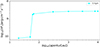 |
Fig. 23. Integrated L-band emission for the mean model (cyan) within different radial apertures (dots). The solid line (between the dots) is for guidance. There is a jump at the inner edge of the disk (60 au), where most of the L-band flux is produced. |
We note that during the burst, the sublimation radius is expected to shift outward by a few 10 au. The L-band observation was done nearly a decade after the peak of the burst. This is too short for the material to recondense. Thus, the inner rim at the date of the L-band observations may be further away than ∼20 au. Indeed, for low-mass YSO bursts, dust sublimation fronts are an indirect tracer of past outbursts (see, e.g., Jørgensen et al. 2020). However, for massive protostars, the matter will be replenished quickly, given the high accretion rates. With an accretion rate of 10−3 M⊙ yr−1, it follows that in a decade 10−2 M⊙ can be transported to the inner region, enough to refill the inner disk. If the sublimation radius were still further out, higher fluxes would result from the increased surface area. However, the i-band post- and pre-burst fluxes are the same within the errors. Together, this indicates that there are no significant changes present in the dust distribution in 2023 and that the L-band emission originates at the inner rim of the disk, which seems to be as close as the pre-burst dust sublimation radius.
5.6. Prospects for TDRT modeling of MYSO bursts
The present paper describes the first application of TDRT based on the TORUS code in a real-world case. In that context, we want to outline its potential for the future.
The time-dependent approach we use is only the first step in the direction of a fully self-consistent treatment of outbursts. Improved and more systematic modeling is planned for existing FIR bursts (including G323). The next step is to use larger sets of time-dependent models, which all agree with the pre-burst. With this in mind, the previous parameter ranges (for both burst and MYSO geometry) shall be refined in the near future. Due to the SOFIA shutdown, no further FIR observations will be possible in the mid-term. However, future MYSO bursts can be studied with ground-based facilities in the (sub)mm and in the NIR/MIR provided the burst hosts are no longer deeply embedded. JWST is capable of targeting younger and more enshrouded objects.
With TORUS the dust continuum can be modeled in those spectral ranges as well, while line emission is currently not included in the time-dependent version. The temperature grids are delivered at each time step. They might be used as input for chemical burst models, similar to the approach used in Rab et al. (2017), Guadarrama et al. (2024). TORUS does not include chemical networks, which are needed to directly obtain chemical burst models. Another application of the temperature output is to constrain the location of possible methanol maser sites. This was done in a simplified manner by Stecklum et al. (2021) for static model grids.
For all our models, we used very simplified assumptions, namely no protostellar bloating, axis-symmetry, same dust in all regions and no changes during the burst besides heating and cooling (i.e., no changes in the dust distribution and chemistry due to sublimation, etc.). Some of these limitations might be explored in the future. A simple form of dust sublimation is included in which a fraction of the dust exceeding the sublimation temperature is removed each time step. Currently, resublimation is immediate once the temperature drops below the sublimation temperature. This might be improved in the future. Eventually, we emphasize that TDRT can be applied to other classes of variable objects and transient phenomena where dust plays a major role.
6. Conclusions
G323 featured a powerful accretion burst that peaked in 2013. It extends the small sample of known MYSO bursts. The objective of this work is to draw conclusions about the nature of the burst from the derived limits for the released energy and the accreted mass. G323’s burst is a multiwavelength phenomenon that was accompanied by flares of different maser species. It was observed in the NIR, MIR, FIR, and radio at different timescales. There is a clear correlation between the Class II methanol maser flare and the IR radiation. A light echo is present in J, H, Ks, and Z as well as in the WISE images. Interestingly, its expansion appears to be faster at longer wavelengths, possibly because at these wavelengths the scattering optical depth is reduced.
Our SOFIA/HAWC+ observations, performed in 2022, two years after the end of the burst, constrained the strength of the thermal afterglow and were crucial to derive limits on the burst energy. These measurements and the Ks light curve from the VVV(X) survey, indicate that the burst is probably the most energetic of all known MYSO bursts. The energy released is equal to  . Its duration, i.e, 8.4 yr, is in line with the accretion of a compact object. This is in accordance with the observed bluening during the burst, which is not expected if the material flow arises in a more diffuse stream from an active disk. For a protostar close to the ZAMS, the minimum mass needed to release this amount of energy is
  times the Jupiter mass, which is in the range of a big Jupiter, a brown dwarf, or a disk fragment. The pre-burst luminosity of G323 is consistent with that of a bloated protostar, which might feature pulsations with the same period as the maser. If the bloating scenario holds, the accreted mass may be as high as half a solar mass. The post-burst emission in the L-band can be attributed to the inner disk region. It indicates a minimum extent of the emitting region of 14 mas or 57 au, which is consistent with a disk inner rim situated at the dust sublimation radius during quiescence.
For the first time, we used time-dependent radiative transfer (TDRT) to study a real science case. With TDRT, we can model the timescales self-consistently. The thermal afterglow is much longer than the grid crossing time. G323 is most likely seen face-on. Therefore, the NIR timescales are equal to those of the accretion rate variation. The Ks light curve reflects the protostellar luminosity variation throughout the entire burst duration. At longer wavelengths, the timescales are much longer. We find that the visibility of the (MIR/FIR) afterglow can vary by up to years, depending on the dust distribution and the burst characteristics. The example of G323 shows that TDRT simulations are a powerful tool for investigating transient phenomena of dusty objects. For episodic accretion of MYSO, it opens up the possibility to obtain reliable burst parameters, which are needed to understand the unsteady protostellar growth, especially in the high-mass regime. The shutdown of SOFIA is a serious drawback, since it was the only facility that could observe in the FIR which is crucial to derive the burst energy. Future studies must focus on MIR and (sub)mm. The rare face-on view of G323 and its NIR record of the burst make this source a key object for studying the consequences of episodic accretion and a benchmark for the corresponding simulations.
IRAF (Image Reduction and Analysis Facility) is distributed by the National Optical Astronomy Observatories, which are operated by AURA, Inc., in cooperative agreement with the National Science Foundation.
IDL® is a registered trademark of L3Harris Technologies, Inc.
Acknowledgments
We thank the anonymous referee for accurate review and highly appreciate comments and suggestions which helped to improve the quality of this paper. The authors thank Dr. Gordon MacLeod for support concerning the maser observations and Dr. Riccardo Cesaroni for input concerning the free–free emission luminosity. V.W. was supported by the German Aerospace Center (DLR) under grant number 50OR1718. A.C.G. acknowledges from PRIN-MUR 2022 20228JPA3A “The path to star and planet formation in the JWST era (PATH)” funded by NextGeneration EU and by INAF-GoG 2022 “NIR-dark Accretion Outbursts in Massive Young Stellar Objects (NAOMY)” and Large Grant INAF 2022 “YSOs, Outflows, Disks, and Accretion: toward a global framework for the evolution of planet-forming systems (YODA)”. This publication uses data products from the Near-Earth Object Wide-field Infrared Survey Explorer ((NEO)WISE), which is a joint project of the Jet Propulsion Laboratory/California Institute of Technology and the University of Arizona. (NEO)WISE is funded by the National Aeronautics and Space Administration. Based on data products from observations made with ESO Telescopes at the La Silla or Paranal Observatories under ESO programmes 083.C-0582, 179.B-2002 and 198.B-2004. Based on data obtained from the ESO Science Archive Facility under request numbers 557557 and 573746. The ALMA data are from the programme ALMAGAL (2019.1.00195.L) and were retrieved from the ALMA Science Archive (e.g., Stoehr et al. 2014). This paper used information from the Red MSX Source survey database at http://rms.leeds.ac.uk/cgi-bin/public/RMS_DATABASE.cgi, which was constructed with the support of the Science and Technology Facilities Council of the UK. This work used data from the European Space Agency (ESA) mission Gaia (https://www.cosmos.esa.int/gaia), processed by the Gaia Data Processing and Analysis Consortium (DPAC, https://www.cosmos.esa.int/web/gaia/dpac/consortium). Funding for the DPAC has been provided by national institutions, in particular, the institutions participating in the Gaia Multilateral Agreement. The national facility capability for SkyMapper has been funded through ARC LIEF grant LE130100104 from the Australian Research Council, awarded to the University of Sydney, the Australian National University, Swinburne University of Technology, the University of Queensland, the University of Western Australia, the University of Melbourne, Curtin University of Technology, Monash University and the Australian Astronomical Observatory. SkyMapper is owned and operated by The Australian National University’s Research School of Astronomy and Astrophysics. Survey data were processed and provided by the SkyMapper Team at ANU. This research has made use of NASA’s Astrophysics Data System. This research has used adstex (https://github.com/yymao/adstex).
References
- Ahmadi, A., Beuther, H., Bosco, F., et al. 2023, A&A, 677, A171 [NASA ADS] [CrossRef] [EDP Sciences] [Google Scholar]
- Alard, C., & Lupton, R. H. 1998, ApJ, 503, 325 [Google Scholar]
- Amôres, E. B., & Lépine, J. R. D. 2005, AJ, 130, 659 [CrossRef] [Google Scholar]
- Araya, E., Hofner, P., Kurtz, S., Bronfman, L., & DeDeo, S. 2005, ApJS, 157, 279 [NASA ADS] [CrossRef] [Google Scholar]
- Audard, M., Ábrahám, P., Dunham, M. M., et al. 2014, in Protostars and Planets VI, eds. H. Beuther, R. S. Klessen, C. P. Dullemond, T. Henning, 387 [Google Scholar]
- Bailer-Jones, C. A. L., Rybizki, J., Fouesneau, M., Mantelet, G., & Andrae, R. 2018, AJ, 156, 58 [Google Scholar]
- Bayandina, O. S., Brogan, C. L., Burns, R. A., et al. 2022, A&A, 664, A44 [NASA ADS] [CrossRef] [EDP Sciences] [Google Scholar]
- Beuther, H., Ahmadi, A., Mottram, J. C., et al. 2019, A&A, 621, A122 [NASA ADS] [CrossRef] [EDP Sciences] [Google Scholar]
- Bøgelund, E. G., McGuire, B. A., Hogerheijde, M. R., van Dishoeck, E. F., & Ligterink, N. F. W. 2019, A&A, 624, A82 [EDP Sciences] [Google Scholar]
- Bordier, E., de Wit, W. J., Frost, A. J., et al. 2024, A&A, 681, A85 [NASA ADS] [CrossRef] [EDP Sciences] [Google Scholar]
- Breen, S. L., Ellingsen, S. P., Contreras, Y., et al. 2013, MNRAS, 435, 524 [Google Scholar]
- Brogan, C. L., Hunter, T. R., Cyganowski, C. J., et al. 2018, ApJ, 866, 87 [NASA ADS] [CrossRef] [Google Scholar]
- Brogan, C. L., Hunter, T. R., Towner, A. P. M., et al. 2019, ApJ, 881, L39 [NASA ADS] [CrossRef] [Google Scholar]
- Burns, R. A., Sugiyama, K., Hirota, T., et al. 2020, Nat. Astron., 4, 506 [Google Scholar]
- Burns, R. A., Uno, Y., Sakai, N., et al. 2023, Nat. Astron., 7, 634 [NASA ADS] [CrossRef] [Google Scholar]
- Cantat-Gaudin, T., Jordi, C., Vallenari, A., et al. 2018, A&A, 618, A93 [NASA ADS] [CrossRef] [EDP Sciences] [Google Scholar]
- Caratti o Garatti, A., Stecklum, B., Linz, H., Garcia Lopez, R., & Sanna, A. 2015, A&A, 573, A82 [NASA ADS] [CrossRef] [EDP Sciences] [Google Scholar]
- Caratti o Garatti, A., Stecklum, B., Garcia Lopez, R., et al. 2017, Nat. Phys., 13, 276 [Google Scholar]
- Caswell, J. L. 1997, MNRAS, 289, 203 [NASA ADS] [CrossRef] [Google Scholar]
- Caswell, J. L., & Reynolds, J. E. 2001, MNRAS, 325, 1346 [NASA ADS] [CrossRef] [Google Scholar]
- Cesaroni, R., Pestalozzi, M., Beltrán, M. T., et al. 2015, A&A, 579, A71 [NASA ADS] [CrossRef] [EDP Sciences] [Google Scholar]
- Cesaroni, R., Sánchez-Monge, Á., Beltrán, M. T., et al. 2016, A&A, 588, L5 [NASA ADS] [CrossRef] [EDP Sciences] [Google Scholar]
- Cesaroni, R., Moscadelli, L., Neri, R., et al. 2018, A&A, 612, A103 [NASA ADS] [CrossRef] [EDP Sciences] [Google Scholar]
- Chen, X., Sobolev, A. M., Ren, Z.-Y., et al. 2020, Nat. Astron., 4, 1170 [Google Scholar]
- Chen, Z., Sun, W., Chini, R., et al. 2021, ApJ, 922, 90 [NASA ADS] [CrossRef] [Google Scholar]
- Chiang, E. I., & Goldreich, P. 1997, ApJ, 490, 368 [Google Scholar]
- Contreras Peña, C., Johnstone, D., Baek, G., et al. 2020, MNRAS, 495, 3614 [Google Scholar]
- Contreras Peña, C., Ashraf, M., Lee, J.-E., et al. 2023, J. Korean Astron. Soc., 56, 253 [Google Scholar]
- Cragg, D. M., Sobolev, A. M., & Godfrey, P. D. 2005, MNRAS, 360, 533 [Google Scholar]
- Csengeri, T., Bontemps, S., Wyrowski, F., et al. 2017, A&A, 601, A60 [NASA ADS] [CrossRef] [EDP Sciences] [Google Scholar]
- Cutri, R. M., Wright, E. L., Conrow, T., et al. 2014, VizieR Online Data Catalog: II/328 [Google Scholar]
- Dahm, S. E., & Hillenbrand, L. A. 2017, AJ, 154, 177 [NASA ADS] [CrossRef] [Google Scholar]
- Dawson, R. I., & Johnson, J. A. 2018, ARA&A, 56, 175 [Google Scholar]
- Draine, B. T. 2003, ApJ, 598, 1017 [NASA ADS] [CrossRef] [Google Scholar]
- Elbakyan, V. G., Nayakshin, S., Vorobyov, E. I., Caratti o Garatti, A.& Eislöffel, J. 2021, A&A, 651, L3 [NASA ADS] [CrossRef] [EDP Sciences] [Google Scholar]
- Elbakyan, V. G., Nayakshin, S., Meyer, D. M. A., & Vorobyov, E. I. 2023, MNRAS, 518, 791 [Google Scholar]
- Elia, D., Molinari, S., Schisano, E., et al. 2017, MNRAS, 471, 100 [NASA ADS] [CrossRef] [Google Scholar]
- Erickson, E. F., & Davidson, J. A. 1993, Adv. Space Res., 13, 549 [Google Scholar]
- Esau, C. F., Harries, T. J., & Bouvier, J. 2014, MNRAS, 443, 1022 [NASA ADS] [CrossRef] [Google Scholar]
- Fischer, W. J., Battersby, C., Johnstone, D., et al. 2024, AJ, 167, 82 [NASA ADS] [CrossRef] [Google Scholar]
- Gaia Collaboration (Brown, A. G. A., et al.) 2018, A&A, 616, A1 [NASA ADS] [CrossRef] [EDP Sciences] [Google Scholar]
- Gaia Collaboration (Brown, A. G. A., et al.) 2021, A&A, 649, A1 [NASA ADS] [CrossRef] [EDP Sciences] [Google Scholar]
- Green, J. A., Caswell, J. L., & McClure-Griffiths, N. M. 2015, MNRAS, 451, 74 [NASA ADS] [CrossRef] [Google Scholar]
- Guadarrama, R., Vorobyov, E. I., Rab, C., et al. 2024, A&A, 684, A51 [NASA ADS] [CrossRef] [EDP Sciences] [Google Scholar]
- Guerra-Varas, N., Merello, M., Bronfman, L., et al. 2023, A&A, 677, A148 [NASA ADS] [CrossRef] [EDP Sciences] [Google Scholar]
- Guo, Z., Lucas, P. W., Kurtev, R. G., et al. 2024, MNRAS, 529, L115 [Google Scholar]
- Harper, D. A., Runyan, M. C., Dowell, C. D., et al. 2018, J. Astron. Instrum., 7, 1840008 [Google Scholar]
- Harries, T. J. 2011, MNRAS, 416, 1500 [Google Scholar]
- Harries, T. J., Haworth, T. J., Acreman, D., Ali, A., & Douglas, T. 2019, Astron. Comput., 27, 63 [NASA ADS] [CrossRef] [Google Scholar]
- Hartmann, L., & Kenyon, S. J. 1996, ARA&A, 34, 207 [NASA ADS] [CrossRef] [Google Scholar]
- Haynes, R. F., Caswell, J. L., & Simons, L. W. J. 1978, Aust. J. Phys. Astrophys. Suppl., 45, 1 [NASA ADS] [Google Scholar]
- Herbig, G. H. 1977, ApJ, 217, 693 [NASA ADS] [CrossRef] [Google Scholar]
- Hodapp, K. W., & Chini, R. 2015, ApJ, 813, 107 [NASA ADS] [CrossRef] [Google Scholar]
- Hollenbach, D., Johnstone, D., Lizano, S., & Shu, F. 1994, ApJ, 428, 654 [NASA ADS] [CrossRef] [Google Scholar]
- Hosokawa, T., Yorke, H. W., & Omukai, K. 2010, ApJ, 721, 478 [Google Scholar]
- Hunter, T. R., Brogan, C. L., MacLeod, G., et al. 2017, ApJ, 837, L29 [NASA ADS] [CrossRef] [Google Scholar]
- Hunter, T. R., Brogan, C. L., MacLeod, G. C., et al. 2018, ApJ, 854, 170 [NASA ADS] [CrossRef] [Google Scholar]
- Hunter, T. R., Brogan, C. L., De Buizer, J. M., et al. 2021, ApJ, 912, L17 [CrossRef] [Google Scholar]
- Inayoshi, K., Sugiyama, K., Hosokawa, T., Motogi, K., & Tanaka, K. E. I. 2013, ApJ, 769, L20 [Google Scholar]
- Jarrett, T. H., Chester, T., Cutri, R., et al. 2000, AJ, 119, 119 [Google Scholar]
- Jiang, N., Dou, L., Wang, T., et al. 2016, ApJ, 828, L14 [Google Scholar]
- Johnstone, D., Hendricks, B., Herczeg, G. J., & Bruderer, S. 2013, ApJ, 765, 133 [Google Scholar]
- Joint Iras Science, W. G. 1994, VizieR Online Data Catalog: II/125 [Google Scholar]
- Joint IRAS Science Working Group 1997, VizieR Online Data Catalog: III/197 [Google Scholar]
- Jørgensen, J. K., Belloche, A., & Garrod, R. T. 2020, ARA&A, 58, 727 [Google Scholar]
- Karska, A., Herpin, F., Bruderer, S., et al. 2014, A&A, 562, A45 [NASA ADS] [CrossRef] [EDP Sciences] [Google Scholar]
- Kervella, P., Mérand, A., Szabados, L., et al. 2008, A&A, 480, 167 [NASA ADS] [CrossRef] [EDP Sciences] [Google Scholar]
- Kim, W. J., Urquhart, J. S., Wyrowski, F., Menten, K. M., & Csengeri, T. 2018, A&A, 616, A107 [CrossRef] [EDP Sciences] [Google Scholar]
- Krieger, A., & Wolf, S. 2021, A&A, 645, A143 [NASA ADS] [CrossRef] [EDP Sciences] [Google Scholar]
- Landsman, W. B. 1995, in Astronomical Data Analysis Software and Systems IV, eds. R. A. Shaw, H. E. Payne, & J. J. E. Hayes, ASP Conf. Ser., 77, 437 [NASA ADS] [Google Scholar]
- Lee, J.-E. 2007, J. Korean Astron. Soc., 40, 83 [CrossRef] [Google Scholar]
- Lenzen, R., Hartung, M., Brandner, W., et al. 2003, in Instrument Design and Performance for Optical/Infrared Ground-based Telescopes, eds. M. Iye, & A. F. M. Moorwood, SPIE Conf. Ser., 4841, 944 [NASA ADS] [CrossRef] [Google Scholar]
- Li, S., Sanhueza, P., Beuther, H., et al. 2024, Nat. Astron., 8, 472 [NASA ADS] [CrossRef] [Google Scholar]
- Liu, T., Evans, N. J., Kim, K.-T., et al. 2020a, MNRAS, 496, 2790 [Google Scholar]
- Liu, S.-Y., Su, Y.-N., Zinchenko, I., et al. 2020b, ApJ, 904, 181 [Google Scholar]
- Lopez, B., Lagarde, S., Petrov, R. G., et al. 2022, A&A, 659, A192 [NASA ADS] [CrossRef] [EDP Sciences] [Google Scholar]
- Lucas, P. W., Smith, L. C., Guo, Z., et al. 2024, MNRAS, 528, 1789 [NASA ADS] [CrossRef] [Google Scholar]
- Lucy, L. B. 1999, A&A, 344, 282 [NASA ADS] [Google Scholar]
- Lumsden, S. L., Hoare, M. G., Urquhart, J. S., et al. 2013, VizieR Online Data Catalog: J/ApJS/208/11 [Google Scholar]
- Ma, Y., Zhou, J., Esimbek, J., et al. 2023, A&A, 676, A15 [NASA ADS] [CrossRef] [EDP Sciences] [Google Scholar]
- MacLeod, G. C., Gaylard, M. J., & Nicolson, G. D. 1992, MNRAS, 254, 1P [NASA ADS] [CrossRef] [Google Scholar]
- MacLeod, G. C., Sugiyama, K., Hunter, T. R., et al. 2019, MNRAS, 489, 3981 [NASA ADS] [CrossRef] [Google Scholar]
- MacLeod, G. C., Smits, D. P., Green, J. A., & van den Heever, S. P. 2021, MNRAS, 502, 5658 [NASA ADS] [CrossRef] [Google Scholar]
- Magnelli, B., Popesso, P., Berta, S., et al. 2013, A&A, 553, A132 [NASA ADS] [CrossRef] [EDP Sciences] [Google Scholar]
- Mainzer, A., Bauer, J., Cutri, R. M., et al. 2014, ApJ, 792, 30 [Google Scholar]
- Martín-Hernández, N. L., Vermeij, R., & van der Hulst, J. M. 2005, A&A, 433, 205 [NASA ADS] [CrossRef] [EDP Sciences] [Google Scholar]
- Marton, G., Calzoletti, L., Perez Garcia, A. M., et al. 2017, ArXiv e-prints [arXiv:1705.05693] [Google Scholar]
- Masci, F. 2013, Astrophysics Source Code Library [record ascl:1302.010] [Google Scholar]
- Mathis, J. S., Rumpl, W., & Nordsieck, K. H. 1977, ApJ, 217, 425 [Google Scholar]
- McMullin, J. P., Waters, B., Schiebel, D., Young, W., & Golap, K. 2007, in Astronomical Data Analysis Software and Systems XVI, eds. R. A. Shaw, F. Hill, & D. J. Bell, ASP Conf. Ser., 376, 127 [Google Scholar]
- Menten, K. M. 1991a, in Atoms, Ions and Molecules: New Results in Spectral Line Astrophysics, eds. A. D. Haschick, & P. T. P. Ho, ASP Conf. Ser., 16, 119 [NASA ADS] [Google Scholar]
- Menten, K. M. 1991b, ApJ, 380, L75 [Google Scholar]
- Merello, M., Molinari, S., Rygl, K. L. J., et al. 2019, MNRAS, 483, 5355 [NASA ADS] [CrossRef] [Google Scholar]
- Miller, J. P., Pennypacker, C. R., & White, G. L. 2008, PASP, 120, 449 [NASA ADS] [CrossRef] [Google Scholar]
- Min, M. 2015, in Summer School – Protoplanetary Disks: Theory and Modeling Meet Observations, eds. I. Kamp, P. Woitke, & J. D. Ilee, EPJ Web Conf., 102, 00005 [Google Scholar]
- Minniti, D., Lucas, P. W., Emerson, J. P., et al. 2010, New A, 15, 433 [Google Scholar]
- Minniti, D., Lucas, P., & VVV Team 2017, VizieR Online Data Catalog: II/348 [Google Scholar]
- Moffat, A. F. J. 1969, A&A, 3, 455 [NASA ADS] [Google Scholar]
- Mosoni, L., Sipos, N., Ábrahám, P., et al. 2013, A&A, 552, A62 [NASA ADS] [CrossRef] [EDP Sciences] [Google Scholar]
- Mottram, J. C., Hoare, M. G., Lumsden, S. L., et al. 2007, A&A, 476, 1019 [NASA ADS] [CrossRef] [EDP Sciences] [Google Scholar]
- Murphy, T., Cohen, M., Ekers, R. D., et al. 2010, MNRAS, 405, 1560 [Google Scholar]
- Nayakshin, S., & Lodato, G. 2012, MNRAS, 426, 70 [Google Scholar]
- Nemiroff, R. J., Zhong, Q., & Lilleskov, E. 2016, Phys. Educ., 51, 043005 [NASA ADS] [CrossRef] [Google Scholar]
- Noriega-Crespo, A., Morris, P., Marleau, F. R., et al. 2004, ApJS, 154, 352 [NASA ADS] [CrossRef] [Google Scholar]
- Olech, M., Durjasz, M., Szymczak, M., & Bartkiewicz, A. 2022, A&A, 661, A114 [NASA ADS] [CrossRef] [EDP Sciences] [Google Scholar]
- Oliva, G. A., & Kuiper, R. 2020, A&A, 644, A41 [NASA ADS] [CrossRef] [EDP Sciences] [Google Scholar]
- Onken, C. A., Wolf, C., Bessell, M. S., et al. 2024, ArXiv e-prints [arXiv:2402.02015] [Google Scholar]
- Ortiz, J. L., Sugerman, B. E. K., de La Cueva, I., et al. 2010, A&A, 519, A7 [NASA ADS] [CrossRef] [EDP Sciences] [Google Scholar]
- Ostrovskii, A. B., & Sobolev, A. M. 2002, in Cosmic Masers: From Proto-Stars to Black Holes, eds. V. Migenes, & M. J. Reid, 206, 183 [NASA ADS] [Google Scholar]
- Pascucci, I., Wolf, S., Steinacker, J., et al. 2004, A&A, 417, 793 [NASA ADS] [CrossRef] [EDP Sciences] [Google Scholar]
- Pringle, J. E. 1981, ARA&A, 19, 137 [NASA ADS] [CrossRef] [Google Scholar]
- Proven-Adzri, E., MacLeod, G. C., Heever, S. P. V. D., et al. 2019, MNRAS, 487, 2407 [Google Scholar]
- Rab, C., Elbakyan, V., Vorobyov, E., et al. 2017, A&A, 604, A15 [NASA ADS] [CrossRef] [EDP Sciences] [Google Scholar]
- Reid, M. J., Menten, K. M., Brunthaler, A., et al. 2014, ApJ, 783, 130 [Google Scholar]
- Reimann, H. G., Linz, H., Wagner, R., et al. 2000, in Optical and IR Telescope Instrumentation and Detectors, eds. M. Iye, & A. F. Moorwood, SPIE Conf. Ser., 4008, 1132 [NASA ADS] [CrossRef] [Google Scholar]
- Reipurth, B., & Aspin, C. 2004, ApJ, 606, L119 [NASA ADS] [CrossRef] [Google Scholar]
- Robitaille, T. P. 2017, A&A, 600, A11 [NASA ADS] [CrossRef] [EDP Sciences] [Google Scholar]
- Rousset, G., Lacombe, F., Puget, P., et al. 2003, in Adaptive Optical System Technologies II, eds. P. L. Wizinowich, & D. Bonaccini, SPIE Conf. Ser., 4839, 140 [Google Scholar]
- Schuller, F., Menten, K. M., Contreras, Y., et al. 2009, A&A, 504, 415 [NASA ADS] [CrossRef] [EDP Sciences] [Google Scholar]
- Shakura, N. I., & Sunyaev, R. A. 1973, A&A, 24, 337 [NASA ADS] [Google Scholar]
- Sobolev, A. M., Cragg, D. M., & Godfrey, P. D. 1997, A&A, 324, 211 [NASA ADS] [Google Scholar]
- Song, S.-M., Chen, X., Shen, Z.-Q., et al. 2023, ApJS, 265, 16 [NASA ADS] [CrossRef] [Google Scholar]
- Stecklum, B., & Linz, H. 2022, ATel, 15302, 1 [NASA ADS] [Google Scholar]
- Stecklum, B., Heese, S., Wolf, S., et al. 2017, ArXiv e-prints [arXiv:1712.01451] [Google Scholar]
- Stecklum, B., Caratti o Garatti, A., Hodapp, K., et al. 2018, in Astrophysical Masers: Unlocking the Mysteries of the Universe, eds. A. Tarchi, M. J. Reid, & P. Castangia, 336, 37 [NASA ADS] [Google Scholar]
- Stecklum, B., Wolf, V., Linz, H., et al. 2021, A&A, 646, A161 [EDP Sciences] [Google Scholar]
- Stoehr, F., Lacy, M., Leon, S., et al. 2014, in Observatory Operations: Strategies, Processes, and Systems V, eds. A. B. Peck, C. R. Benn, & R. L. Seaman, SPIE Conf. Ser., 9149, 914902 [NASA ADS] [CrossRef] [Google Scholar]
- Sugerman, B. E. K. 2007, in The Nature of V838 Mon and its Light Echo, eds. R. L. M. Corradi, & U. Munari, ASP Conf. Ser., 363, 121 [NASA ADS] [Google Scholar]
- Sugiyama, K., Yonekura, Y., Motogi, K., et al. 2015, PKAS, 30, 129 [NASA ADS] [Google Scholar]
- Sugiyama, K., Saito, Y., Yonekura, Y., & Momose, M. 2019, ATel, 12446, 1 [Google Scholar]
- Szymczak, M., Olech, M., Wolak, P., Gérard, E., & Bartkiewicz, A. 2018, A&A, 617, A80 [NASA ADS] [CrossRef] [EDP Sciences] [Google Scholar]
- Tapia, M., Roth, M., & Persi, P. 2013, Protostars and Planets VI, Poster 1H030 [Google Scholar]
- Tapia, M., Roth, M., & Persi, P. 2015a, MNRAS, 446, 4088 [Google Scholar]
- Tapia, M., Roth, M., & Persi, P. 2015b, MNRAS, 448, 1402 [NASA ADS] [CrossRef] [Google Scholar]
- Tout, C. A., Pols, O. R., Eggleton, P. P., & Han, Z. 1996, MNRAS, 281, 257 [Google Scholar]
- Uchiyama, M., Yamashita, T., Sugiyama, K., et al. 2020, PASJ, 72, 4 [NASA ADS] [CrossRef] [Google Scholar]
- Ulrich, R. K. 1976, ApJ, 210, 377 [Google Scholar]
- Urquhart, J. S., Moore, T. J. T., Csengeri, T., et al. 2014, MNRAS, 443, 1555 [Google Scholar]
- Visser, R., & Bergin, E. A. 2012, ApJ, 754, L18 [NASA ADS] [CrossRef] [Google Scholar]
- Vorobyov, E. I., Baraffe, I., Harries, T., & Chabrier, G. 2013, A&A, 557, A35 [NASA ADS] [CrossRef] [EDP Sciences] [Google Scholar]
- Walsh, A. J., Burton, M. G., Hyland, A. R., & Robinson, G. 1998, MNRAS, 301, 640 [Google Scholar]
- Weingartner, J. C., & Draine, B. T. 2001, ApJ, 548, 296 [Google Scholar]
- Whitney, B. A., Indebetouw, R., Bjorkman, J. E., & Wood, K. 2004, ApJ, 617, 1177 [NASA ADS] [CrossRef] [Google Scholar]
- Wright, E. L., Eisenhardt, P. R. M., Mainzer, A. K., et al. 2010, AJ, 140, 1868 [Google Scholar]
- Yamamura, I. 2010, 38th COSPAR Scientific Assembly, 38, 2 [NASA ADS] [Google Scholar]
- Yamamura, I., Makiuti, S., Ikeda, N., et al. 2009, in AKARI, a Light to Illuminate the Misty Universe, eds. T. Onaka, G. J. White, T. Nakagawa, I. Yamamura (San Francisco: Astronomical Society of the Pacific), ASP Conf. Ser., 418, 3 [NASA ADS] [Google Scholar]
- Yang, A. Y., Urquhart, J. S., Wyrowski, F., et al. 2022, A&A, 658, A160 [NASA ADS] [CrossRef] [EDP Sciences] [Google Scholar]
- Young, E. T., Becklin, E. E., Marcum, P. M., et al. 2012, ApJ, 749, L17 [NASA ADS] [CrossRef] [Google Scholar]
- Zhang, C., Zhu, F.-Y., Liu, T., et al. 2023, MNRAS, 520, 3245 [NASA ADS] [CrossRef] [Google Scholar]
Appendix A: Additional information
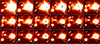 |
Fig. A.1. Evolution of the remote LE (left border) in the W1 band, illustrated by bi-annual difference images that were created by subtracting those from 2014. FoV and orientation correspond to Fig. 6. Each row covers three years, starting on top left in early 2015. The W2 images look similar. A few variable stars are present as well. |
HAWC+ photometry and beam sizes.
(NEO)WISE photometry.
G323 pre-burst flux densities.
Skymapper photometry.
Ks VVV(X) photometry.
G323 pre-burst fit result.
All Tables
All Figures
|
Fig. 1. VVV JHKs pre-burst (left) and burst (right) color composites (FoV 44″ × 44″, north is up and east is to the left). The central cyan-colored areas are due to detector saturation. |
| In the text | |
|
Fig. 2. TIMMI2 10.4 μm image (epoch 2006). The lower left circle shows the FWHM of a standard star measured before the object. The contours delineate [5, 35, 200, 560] × 1σ levels where the latter corresponds to half of the peak value. No Airy-rings are visible, although the source was classified as point-like. |
| In the text | |
|
Fig. 3. HAWC+ log scaled image cutouts, centered on G323 and spatially scaled to the beam FWHM (lower left) for each band. The absence of Airy rings indicates that the source is resolved at all wavelengths. The horizontal line marks an angular size of 1′. |
| In the text | |
|
Fig. 4. Left: light curves based on VVV(X) (black) and (NEO)WISE photometry (W1 – blue, and W2 – red) as well as 6.7 GHz total maser flux (green, Green et al. 2015; MacLeod et al. 2021). Vertical red and blue lines mark the dates of the burst onset and first flare evidence from the 6.035 GHz exOH maser (MacLeod et al. 2021). The Ks rise was approximated by a polynomial, while its decay is roughly linear on a log scale (dashed line). The (NEO)WISE magnitudes are shifted to match those of Ks. The integrated maser flux is shown on a log scale (right ordinate). Its scatter is due to the short-term periodicity. Right: Ks (black), i (blue), and z (green) light curves, with i and z magnitudes shifted to match those of Ks. The z pre- and post-magnitudes agree within the errors. |
| In the text | |
|
Fig. 5. Columns from left to right: Z, Y, J, H, and Ks images and rows from top to bottom: those of 2010, 2015, difference, and ratio (range 0…17.5). The crosshair marks the MYSO position. For the upper two rows, the values comprise 98 percentiles, displayed using a linear stretch. At red optical wavelengths (two leftmost columns), the object appears bipolar. Both blobs are probably due to scattering, with the eastern one brighter in Z. Both are offset from the nominal MYSO position and indicated by the red Z contours in Fig. 10. The prompt LE is visible in all five bands. Its large size in the Ks ratio image is due to a smaller number of scatterings compared to the other bands. A common foreground proper motion binary (blue arrow) appears in Z and J next to G323. The FoV amounts to 70″ × 45″. |
| In the text | |
|
Fig. 6. Ks-band difference images showing the temporal evolution of the burst and the associated LEs, displayed using a log scale. The prompt echo, which originates from the cloud core, is monopolar and spreads to the southeast at an PA of ∼135°. A remote LE that appeared later traces denser structures of the ISM. The red polygon encloses the area from which its light curves were established. The FoV is 135″ × 80″. |
| In the text | |
|
Fig. 7. Light curves of the remote LE where colored error bars denote the following: Ks (black), W1 (blue), W2 (red), and W1 − W2 color (green, right ordinate). The vertical dashed line marks the date of the burst peak. The LE peak occurs slightly more than four years after the burst peak. |
| In the text | |
|
Fig. 8. Flux growth curves of PACS (dashed) and HAWC+ (solid). The wavelength bands are indicated by color, where blue is 62/70 and red 154/160 μm for HAWC+/PACS, respectively. The vertical lines mark the aperture radii, which reproduce the HPPSC fluxes. Black lines are polynomial approximations, reducing the influence of finite pixel size. The mean of the growth curve ratios gives the increase at the HAWC+ epoch. |
| In the text | |
|
Fig. 9. Pre-burst SED (blue), together with the HAWC+ post-burst observations (orange). The HAWC+ observations were interpolated to match the wavelengths of the pre-burst observation. The resulting data points are colored red. The inset shows a zoom-in on the region of interest. The flux excess in the post-burst epoch is small (only ∼10% at 70, 160 μm). |
| In the text | |
|
Fig. 10. NACO AO Ks-band image (epoch 2009) using a logarithmic stretch with contours of the 19 GHz radio continuum (white, Murphy et al. 2010) and from the Z-band pre-burst image (red, epoch 2010). Maser spots are marked by crosses in blue (Caswell & Reynolds 2001, epoch 1994) and red (Green et al. 2015, epoch 2011), with sizes indicating the position error. The black diamond is at the peak of the 1.4 mm emission while the black square marks the Gaia source. The yellow rectangle shows orientation and width of the ISAAC slit. |
| In the text | |
|
Fig. 11. Zoom-in sections of the continuum-subtracted spectral image showing 2.122 μm H2 (left) and 2.166 μm Brγ (right), both featuring extended emission. Red contours show the source continuum emission (1 − 3) × 10−14 erg s−1 cm−2 Å−1. NE is up. |
| In the text | |
|
Fig. 12. 1.4 mm dust continuum map with superimposed contours. The ellipse on the lower left indicates the beam size. The object is resolved and shows faint extended emission. |
| In the text | |
|
Fig. 13. First moment of the SiO emission with superimposed dust continuum contours from the ALMA 12-m array. The color bar indicates the velocity interval, in units of km s−1. There is a slight gradient from the SE to the NW. |
| In the text | |
|
Fig. 14. Distribution of the redshifted and blueshifted 13CO (2–1) line emission as mapped with the ALMA 12-m Array superimposed on a Ks image taken in mid-2015. The synthesized ALMA beam size for the line observations is shown in the lower left. The compact 1.4 mm emission, mapped at much higher resolution, appears as a small blob within the white saturated pixels. |
| In the text | |
|
Fig. 15. All TORUS models (gray), together with the pre-burst SED (blue dots), the ten best fits (blue, the best one is darkest), and the mean model (red). The model SEDs are reddened according to the foreground extinction of 18 mag (Murphy et al. 2010). Background colors indicate different wavelength ranges. The SED peaks in the MIR/FIR. The wavelength range of HAWC+ is indicated at the bottom. That for radiative maser excitation (Ostrovskii & Sobolev 2002) is highlighted in blue. Flux densities are listed in Table A.3. The mean model fits the pre-burst SED quite well. |
| In the text | |
|
Fig. 16. Dynamic SED showing the flux density over wavelength and time (increasing from top to bottom) of the mean-setting and a burst with an energy of 2.3 × 1047 erg. Time 0 marks the onset of the burst. Horizontal lines indicate the peak time (white triangles), the time when 80% of the energy is released in the respective band (black dots), and when the flux increase is back at 1.25 times the pre-burst level (gray crosses). The increase in scatter in the (sub)mm range is due to lower synthetic photon counts. |
| In the text | |
|
Fig. 17. Input burst profiles (left) and output flux ratios as a function of time for 70 (middle) and 160 μm (right) for the mean model. The burst energy is varied between (0.23 and 6.9)×1047 erg (color-coded). Obviously, the afterglows are longer for more energetic bursts. The geometry is the same for all simulations. The HAWC+ measurements are colored red. The horizontal solid and dashed-dotted lines mark the pre-burst level and 1.25 times that level. The insets show a zoom-in on the region of interest. The simulations (colored dots) were interpolated in time to reduce numerical scatter (corresponding lines and shaded regions). The observations are given in red. |
| In the text | |
|
Fig. 18. Modeled flux ratio at 70 (blue) and 160 μm (red dots) for different burst energies, all featuring the mean setting. Solid lines are linear fits. The dashed horizontal lines are the observations with confidence intervals (overlapping colored areas). The vertical black line indicates the best burst energy Eacc for both wavelengths. The 1σ-confidence interval is indicated. We use a χ2-minimization to determine Eacc, where we use linear fits (colored solid lines) as model values for both wavelengths. We take into account the observational errors and uncertainties of the modeled ratios, where the contribution of the latter is minor. |
| In the text | |
|
Fig. 19. Same as Fig. 16 but for the Tmin (left) and Tmax (right) setting. The burst is the same for both. The plot shows that the dust distribution strongly imprints the afterglow. For denser and more extended envelopes, the MIR/FIR afterglow can be significantly longer. Horizontal lines indicate the times when the peak is reached (white triangles), when 80% of the energy is released (black dots), and the time when the flux density is back at 1.25 × Lpre(λ) (gray). |
| In the text | |
|
Fig. 20. Same as Fig. 18, but for the Tmin and Tmax model (top and bottom, respectively). For these settings, the burst energy (indicated by the vertical black line) needed to explain the HAWC+ data (horizontal red and blue lines) is maximized or minimized respectively. Interestingly, for the Tmax setting, which is the most extended and densest, the flux ratio at 160 μm (red) exceeds that at 70 μm (blue). The dependency is almost linear. The best fits are indicated by the solid colored lines. Note the different scales. |
| In the text | |
|
Fig. 21. Modeled Ks ratio curve for the Tmin (left), mean (middle), and Tmax (right) model setups featuring different bursts (in 1047 erg, color-coded). The observed Ks increase is shown in red for comparison. The ratio depends more on the energy input than on the setting. The best agreement is reached for Eacc = 0.93 × 1047 erg. For the Tmin setting and the highest burst energies, the Ks curves decay delayed, this might be an artifact due to the innermost dust becoming unrealistically hot (rmin is fixed to 60 au, that is, 3 × Rsub). We note that the ordinate scales are different. |
| In the text | |
|
Fig. 22. Predicted Ks ratio for the mean model with (blue) and without (black) dust sublimation. Without dust sublimation, the increase is overpredicted by a factor of ∼1.5. |
| In the text | |
|
Fig. 23. Integrated L-band emission for the mean model (cyan) within different radial apertures (dots). The solid line (between the dots) is for guidance. There is a jump at the inner edge of the disk (60 au), where most of the L-band flux is produced. |
| In the text | |
|
Fig. A.1. Evolution of the remote LE (left border) in the W1 band, illustrated by bi-annual difference images that were created by subtracting those from 2014. FoV and orientation correspond to Fig. 6. Each row covers three years, starting on top left in early 2015. The W2 images look similar. A few variable stars are present as well. |
| In the text | |
Current usage metrics show cumulative count of Article Views (full-text article views including HTML views, PDF and ePub downloads, according to the available data) and Abstracts Views on Vision4Press platform.
Data correspond to usage on the plateform after 2015. The current usage metrics is available 48-96 hours after online publication and is updated daily on week days.
Initial download of the metrics may take a while.