| Issue |
A&A
Volume 687, July 2024
|
|
|---|---|---|
| Article Number | A43 | |
| Number of page(s) | 14 | |
| Section | Extragalactic astronomy | |
| DOI | https://doi.org/10.1051/0004-6361/202349050 | |
| Published online | 25 June 2024 | |
Physical properties of the southwest outflow streamer in the starburst galaxy NGC 253 with ALCHEMI
1
Institute of Astronomy, Graduate School of Science, The University of Tokyo, 2-21-1 Osawa, Mitaka, Tokyo 181-0015, Japan
e-mail: This email address is being protected from spambots. You need JavaScript enabled to view it.
2
School of Astronomy and Space Science, Nanjing University, Nanjing 210023, PR China
3
School of Physics and Technology, Nanjing Normal University, Nanjing 210023, PR China
4
National Astronomical Observatory of Japan, 2-21-1 Osawa, Mitaka, Tokyo 181-8588, Japan
e-mail: This email address is being protected from spambots. You need JavaScript enabled to view it.
5
Department of Astronomy, School of Science, The Graduate University for Advanced Studies (SOKENDAI), 2-21-1 Osawa, Mitaka, Tokyo 181-1855, Japan
6
ALMA Project, National Astronomical Observatory of Japan, 2-21-1, Osawa, Mitaka, Tokyo 181-8588, Japan
7
Department of Physics, Faculty of Science and Technology, Keio University, 3-14-1 Hiyoshi, Yokohama, Kanagawa 223–8522, Japan
8
European Southern Observatory, Alonso de Córdova, 3107, Vitacura, Santiago 763-0355, Chile
9
Joint ALMA Observatory, Alonso de Córdova, 3107, Vitacura, Santiago 763-0355, Chile
10
National Radio Astronomy Observatory, 520 Edgemont Road, Charlottesville, VA 22903-2475, USA
11
Institute of Astronomy and Astrophysics, Academia Sinica, 11F of AS/NTU Astronomy-Mathematics Building, No.1, Sec. 4, Roosevelt Rd, Taipei 10617, Taiwan
12
Department of Space, Earth and Environment, Chalmers University of Technology, Onsala Space Observatory, 439 92 Onsala, Sweden
13
Leiden Observatory, Leiden University, PO Box 9513 2300 RA Leiden, The Netherlands
14
Centro de Astrobiología (CSIC-INTA), Ctra. de Ajalvir Km. 4, Torrejón de Ardoz, 28850 Madrid, Spain
15
New Mexico Institute of Mining and Technology, 801 Leroy Place, Socorro, NM 87801, USA
16
National Radio Astronomy Observatory, PO Box O, 1003 Lopezville Road, Socorro, NM 87801, USA
17
Max-Planck-Institut für Radioastronomie, Auf dem Hügel 69, 53121 Bonn, Germany
18
Astronomy Department, Faculty of Science, King Abdulaziz University, PO Box 80203 Jeddah 21589, Saudi Arabia
19
Departamento de Astronomia, Instituto de Astronomia, Geofísica e Ciências Atmosféricas da USP, Cidade Universitária, 05508-900 São Paulo, SP, Brazil
Received:
21
December
2023
Accepted:
4
April
2024
Abstract
Aims. The physical properties of galactic molecular outflows are important as they could constrain outflow formation mechanisms. In this work, we study the properties of the southwest (SW) outflow streamer including gas kinematics, optical depth, dense gas fraction, and shock strength through molecular emission in the central molecular zone of the starburst galaxy NGC 253.
Methods. We imaged the molecular emission in NGC 253 at a spatial resolution of 1.6″(∼27 pc at D ∼ 3.5 Mpc) based on data from the ALMA Comprehensive High-resolution Extragalactic Molecular Inventory (ALCHEMI) large program. We traced the velocity and velocity dispersion of molecular gas with the CO(1–0) line and studied the molecular spectra in the region of the SW streamer, the brightest CO streamer in NGC 253. We constrained the optical depth of the CO emission with the CO/13CO(1–0) ratio, the dense gas fraction with the HCN/CO(1–0), H13CN/13CO(1–0) and N2H+/13CO(1–0) ratios, as well as the shock strength with the SiO(2–1)/13CO(1–0) and CH3OH(2k–1k)/13CO(1–0) ratios.
Results. The CO/13CO(1–0) integrated intensity ratio is ∼21 in the SW streamer region, which approximates the C/13C isotopic abundance ratio. The higher integrated intensity ratio compared to the disk can be attributed to the optically thinner environment of CO(1–0) emission inside the SW streamer. The HCN/CO(1–0) and SiO(2–1)/13CO(1–0) integrated intensity ratios both approach ∼0.2 in three giant molecular clouds (GMCs) at the base of the outflow streamers, which implies a higher dense gas fraction and strength of fast shocks in those GMCs than in the disk, while the HCN/CO(1–0) integrated intensity ratio is moderate in the SW streamer region. The contours of those two integrated intensity ratios are extended in the directions of outflow streamers, which connect the enhanced dense gas fraction and shock strength with molecular outflow. Moreover, the molecular gas with an enhanced dense gas fraction and shock strength located at the base of the SW streamer shares the same velocity as the outflow.
Conclusions. The enhanced dense gas fraction and shock strength at the base of the outflow streamers suggest that star formation inside the GMCs can trigger shocks and further drive the molecular outflow. The increased CO/13CO(1–0) integrated intensity ratio coupled with the moderate HCN/CO(1–0) integrated intensity ratio in the SW streamer region are consistent with the picture that the gas velocity gradient inside the streamer may decrease the optical depth of CO(1–0) emission, as well as the dense gas fraction in the extended streamer region.
Key words: galaxies: evolution / galaxies: individual: NGC 253 / galaxies: kinematics and dynamics / galaxies: starburst
© The Authors 2024
 Open Access article, published by EDP Sciences, under the terms of the Creative Commons Attribution License (https://creativecommons.org/licenses/by/4.0), which permits unrestricted use, distribution, and reproduction in any medium, provided the original work is properly cited.
This article is published in open access under the Subscribe to Open model. This email address is being protected from spambots. You need JavaScript enabled to view it. to support open access publication.
1. Introduction
Outflows on a galactic scale are ubiquitous in the local and distant Universe. Together with gas accretion, star formation, and black hole growth, outflows can govern the cycle of material between a galaxy and the circumgalactic medium (Veilleux et al. 2005). Cool outflows, which include atomic and molecular gas, as well as dust, dominate the mass and energy of the outflowing material. The study of extragalactic cool outflows only dates back ∼20 yr; it is a relatively new field in research into galactic outflows (Veilleux et al. 2020). The physical properties of cool outflows are gradually being uncovered thanks to the development of high-capability radio telescopes, including ALMA (ALMA Partnership 2015), NOEMA (Lefèvre et al. 2020), and VLA (Greisen 2003).
As one of the key phases of cool gas, molecular gas is the raw material for star formation, an important process in galaxy evolution. More than 300 molecular species have been detected in the circumstellar envelopes of evolved stars and the interstellar medium (ISM) of the Galaxy1. One third of those species have also been detected in external galaxies (Takano et al. 2019; Martín et al. 2021). Among them, carbon monoxide (CO) is the second most abundant molecule after H2 and serves as the main observational tracer of molecular gas. Moreover, other molecules with different chemical formation pathways and excitation requirements provide supplementary information to constrain the evolution of external galaxies (Aalto 2015).
The formation scenarios for molecular outflows can be roughly divided into three categories. The outflowing molecular gas can be directly driven by radiation (Murray et al. 2011) and/or pressure gradients (Socrates et al. 2008; Uhlig et al. 2012). Alternatively, hot winds can entrain molecular clouds (Banda-Barragán et al. 2019; Fielding & Bryan 2022), while the lifetime of the molecular clouds depends on the balance between radiation, conduction, and turbulence (Orlando et al. 2005). The third scenario is that molecular gas forms in situ from hot winds through cooling and/or thermal instability. The first step in the formation of molecules consists of hydrogen atoms (H) combining to form hydrogen molecules (H2). Given that H atoms can combine on the surface of dust grains, those grains are catalysts for the formation of H2 (Hollenbach & Salpeter 1971; Pantaleone et al. 2021). However, along with temperature rises, dust grains undergo destructive sputtering via gas-grain collisions in the hot winds, which reduces the efficiency of H2 formation (Le Bourlot et al. 2012). Hence, a cooling timescale shorter than a dynamical timescale is a premise for in situ formation (Efstathiou 2000; Silich et al. 2003).
There is no agreement on the influence of outflows on the star formation activity inside host galaxies. On the one hand, the hot ionized winds are one of the leading processes that can quench star formation (Tacchella et al. 2015, 2016; Spilker et al. 2019); namely, negative feedback. The quenching is owing to the energy that is injected into molecular clouds, or to the entrainment or depletion of molecular clouds. On the other hand, the shocks, which form through the encounter between winds and molecular clouds, can compress the molecular clouds and trigger star formation (Klein et al. 1994); namely, positive feedback.
The engines of outflows can be central starbursts and/or active galactic nuclei (AGN). Different physical processes including thermal energy, radiation, cosmic rays, and/or radio jets can work together in either driving mechanism. AGN-driven molecular outflows have been well studied in a few nearby cases such as the Seyfert 2 galaxy NGC 1068 (Kormendy & Ho 2013) and the quasar Mrk 231 (Veilleux et al. 2009). However, to study how molecular outflows relate to star formation, we need to target sources without contamination from AGN.
NGC 253 (D ∼ 3.5 Mpc, Rekola et al. 2005) is one of the nearest starburst galaxies. It possesses a strong bar in the center (Das et al. 2001; Paglione et al. 2004), but shows no sign of AGN activity (Brunthaler et al. 2009). It is an edge-on (i ∼ 78.5°) spiral galaxy and hosts a bipolar outflow (Turner 1985; Westmoquette et al. 2011). The outflow was proven to be driven by the starburst that has been occurring in the central ∼500 pc region for the last ∼20–30 Myr (Rieke et al. 1980; Engelbracht et al. 1998), where the star formation rate is ∼3 M⊙ yr−1 (Ott et al. 2005; Bendo et al. 2015). The outflow has been detected in multiple phases, including the molecular gas phase (Turner 1985; Sturm et al. 2011; Heesen et al. 2011; Bolatto et al. 2013; Walter et al. 2017; Zschaechner et al. 2018; Krieger et al. 2019), the ionized gas phase (Heckman et al. 2000; Westmoquette et al. 2011; Cohen et al. 2020), the X-ray-emitting gas phase (Pietsch et al. 2000; Strickland et al. 2000, 2002; Lopez et al. 2023), and the dust phase (Levy et al. 2022). The ionized outflow shows a wide opening angle of ∼60°, a deprojected velocity of a few 100 km s−1 (Westmoquette et al. 2011), and an extension of ∼10 kpc (Strickland et al. 2002).
There have been several ALMA-based studies of the molecular outflow of NGC 253. Krieger et al. (2019) presented ALMA observations of CO(3–2) in the central 30″ starburst region. They obtained the non-disk component by modeling the disk, deducted the disk from position-velocity diagrams (PVDs), and found that ∼7%–16% of CO luminosity is emitted by the non-disk component. Bolatto et al. (2013) presented ALMA observations of CO(1–0) in the central arcminute, and found the extraplanar molecular gas to be closely tracking the Hα filaments; they estimated the mass outflow rate by assuming an optically thin conversion factor (αCO). By comparing the molecular mass outflow rate (9 M⊙ yr−1) with the star formation rate (2.8 M⊙ yr−1; Ott et al. 2005), Bolatto et al. (2013) concluded that the starburst-driven outflow limits the star formation activity in NGC 253. Zschaechner et al. (2018) presented ALMA observations of CO(1–0) and CO(2–1) in the central 40″ region. They located the molecular outflow via the extended structure in the velocity-integrated intensity map of CO(2–1). Based on the velocity-integrated intensity ratio between CO(2–1) and CO(1–0), they constrained the optical depth of the CO emission in the outflow region. Walter et al. (2017) presented a detailed study of one streamer of the molecular outflow on the southwestern (SW) side – the SW streamer. In addition to the CO emission, they found many bright tracers of dense gas such as HCN, CN, HCO+, and CS in the SW streamer.
This paper is based on the data from the ALMA Comprehensive High-resolution Extragalactic Molecular Inventory (ALCHEMI) project (Martín et al. 2021). The ALCHEMI data targeting the central molecular zone (CMZ) of NGC 253 with a high resolution provide insight into the physical conditions at the center of this galaxy (Haasler et al. 2022). Those data have been used to study the abundance and excitation of different molecular species (Holdship et al. 2021; Harada et al. 2022) in the CMZ of NGC 253, and how they vary with different heating environments (Harada et al. 2021; Holdship et al. 2022; Behrens et al. 2022). In this paper, we uncover the physical properties of the molecular outflow in NGC 253, focusing on the properties of the SW streamer. Taking advantage of the numerous molecular species in the ALCHEMI survey, we study the properties through various integrated intensity ratios. In detail, we use the CO/13CO(1–0) ratio to probe the optical depth (Israel 2020) and HCN/CO(1–0), H13CN/13CO(1–0), and N2H+/13CO(1–0) ratios to probe the dense gas fraction (Gao & Solomon 2004a; Barnes et al. 2020). Moreover, we use SiO(2–1)/13CO(1–0) and CH3OH(2k–1k)/13CO(1–0) ratios to probe the shock strength (García-Burillo et al. 2010).
This paper is organized as follows. The data analysis is presented in Sect. 2. The physical properties of the molecular outflow, including gas kinematics, optical depth, dense gas fraction, and shock strength, are studied in Sect. 3. In Sect. 4, we analyze the correlation between the dense gas fraction and the strength of fast shocks, and discuss how the molecular outflow relates to the star formation in NGC 253. Finally, the results are summarized in Sect. 5.
2. Data analysis
The data used in this study were obtained as part of the ALCHEMI survey, which is an ALMA Cycle 5 large program (2017.1.00161.L). It consists of a wide and unbiased spectral survey covering the CMZ of NGC 253 in Bands 3, 4, 6, and 7. The phase center of observation is α = 00h47m33.26s, δ = −25° 17′17.7″. In this paper, we only make use of the Band 3 data, which covers the ground-state transitions of common molecular lines that can be emitted even from the coldest (∼10 K) medium. We refer readers to Martín et al. (2021) for more details about the data analysis, and only enumerate here the information relevant to this work.
The data cubes from the ALCHEMI survey were imaged to a spatial resolution of 1.6″ (∼27 pc) and a spectral resolution of Δv ∼ 10 km s−1. We uniformly used the continuum-emission-subtracted cubes, which were created by the Python-based tool STATCONT (Sánchez-Monge et al. 2018). Those cubes were primary-beam-corrected in the ALCHEMI imaging process. The Högbom deconvolver function was used for all the cubes from the ALCHEMI survey. Meanwhile, we produced the self-calibrated data cubes with a multi-scale deconvolver function for the integrated intensities of CO and 13CO in the J= 1–0 transition in the ratio map between them. The use of self-calibration allows for a higher signal-to-noise ratio (S/N) and is better for images with complicated spatial structures, which helped us to precisely obtain the optical depth of CO emission in both disk and outflow regions (see Sect. 3.3).
The data cubes from the ALCHEMI survey are subject to the missing flux problem due to the lack of short spacing in interferometric observations. However, the Band 3 observations here probe scales up to ∼30″, while spatial filtering should be relevant to larger scales (Martín et al. 2021). In order to quantify the missing fluxes, we collected the results of IRAM 30m single-dish observations from Aladro et al. (2015). We unified the beam size of the ALCHEMI data cubes to that of the IRAM 30 m observations using the CASA command imsmooth (CASA Team 2022) and compared the integrated intensities between them. All of the missing fluxes of the molecular lines in this work are less than a few percent.
To ensure a sufficient S/N, we masked the region without 3σ-detection. Details of our procedures are as follows. We took the data cubes before primary beam correction, which share the same dimensions as those after primary beam correction, as references. For each targeted molecular line, we masked the region without 3σ-detection for each channel in the corresponding data cube. The integrated intensity, velocity, and velocity dispersion maps – in other words, moment 0, 1, and 2 maps – in the CMZ (inner ∼500 pc) of NGC 253 were generated by the CASA command immoments (CASA Team 2022). The PVDs were generated by the Python-based tool pvextractor (Ginsburg et al. 2016). Given the 3σ-detection limits prior to the analyses, all of the features presented in the following maps and PVDs will be robust.
3. Physical properties of the molecular outflow
3.1. Molecular emission
Figure 1 shows the integrated intensity maps of CO, 13CO, HCN, H13CN, and N2H+ in the J = 1–0 transition and CH3OH (methanol) in the Jk = 2k–1k transition series. We extracted spectral channels covering the 1000 km s−1 velocity range around each transition from the continuum-subtracted cubes, where the rest-frame frequencies are 115.271, 110.201, 88.632, 86.340, 93.174, and ∼96.741 GHz, respectively. The solid black line in Fig. 1a marks the galactic major axis (hereafter major axis) with a position angle of 55°, and was defined following Krieger et al. (2019). The strong CO(1–0) emission in Fig. 1a, which is marked by the blue contour at 4300 K km s−1, is concentrated in the galactic center and distributed along the major axis. Similar structures also exist in other panels of Fig. 1. Das et al. (2001) found that a bar structure along the major axis is necessary to model the ionized gas velocity field in the central ∼100 pc region of NGC 253. A bar structure is also applicable in the CO map in the central ∼300 pc region of NGC 253 (Paglione et al. 2004). A stellar bar, which is known as an efficient mechanism of gas accretion, can trigger strong molecular emission along the major axis, as is seen in Fig. 1. One different point in Fig. 1f from the other panels in Fig. 1 is that the strongest CH3OH(2k–1k) emission exists on the outskirts of the gas disk, suggesting quasi-thermal emission in agreement with Humire et al. (2022).
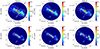 |
Fig. 1. Integrated intensity maps of the transitions used in this work. (a) Integrated intensity map of CO(1–0). The white contour is drawn at 180 K km s−1, the gray contours are drawn at [360, 720, 1440, 2880] K km s−1, and the blue contour is drawn at 4300 K km s−1. The horizontal lines in different colors inside the color bar mark the values of corresponding contours, and remain the same in the following figures. The solid black line marks the major axis, and the dashed black line marks the slice across the SW streamer, on which the black arrows show the positive directions of the PVDs in the following figures. The white arrow points to the SW streamer and remains the same in subsequent panels. The black cross marks the phase center of the observation and remains the same in subsequent figures. The beam size of 1.6″ is shown as an empty black circle in the bottom-left corner of each panel and remains the same in subsequent figures. (b) Integrated intensity map of 13CO(1–0). The gray contours are drawn at [12, 40, 120, 230, 460] K km s−1. (c) Integrated intensity map of HCN(1–0). The gray contours are drawn at [12, 40, 120, 300, 670] K km s−1. (d) Integrated intensity map of H13CN(1–0). The gray contours are drawn at [2, 8, 20, 50, 100] K km s−1. (e) Integrated intensity map of N2H+(1–0). The gray contours are drawn at [5, 20, 50, 100, 200] K km s−1. (f) Integrated intensity map of CH3OH(2k–1k). The gray contours are drawn at [5, 20, 50, 100, 200] K km s−1. |
The CO(1–0) contours (especially the white one at 180 K km s−1) in Fig. 1a are extended toward the SW streamer defined by Walter et al. (2017), which is indicated by a white arrow. A similar extension can be found in the HCN(1–0) contours (Fig. 1c), while the 13CO(1–0) contours are not so extended (Fig. 1b). Based on the ratios between the main and rarer isotopologues, Meier et al. (2015) found that CO(1–0) and HCN(1–0) emission is on average optically thick in the central kpc-scale region of NGC 253. As 13C-bearing molecular species, 13CO(1–0) emission should be moderately optically thin (Martín et al. 2019). The different extensions toward the SW streamer of CO(1–0) and HCN(1–0) emission from the 13CO(1–0) emission imply that the optical depths of CO(1–0) and HCN(1–0) emission in the SW streamer region may be lower than that in the gas disk. Moreover, the fainter emission of H13CN(1–0), N2H+(1–0) and CH3OH(2k–1k) in Figs. 1d, 1e and 1f share similar extensions toward the SW streamer with 13CO(1–0).
Figure 2 shows the intensities of five molecular lines from Fig. 1 and SiO in the J = 2–1 transition (∼86.847 GHz, see Huang et al. 2023 for its integrated intensity map) in the PVDs along the major axis, with systemic velocity reserved and distance referenced from the phase center. The CO(1–0) PVD in Fig. 2a mainly follows a rotating pattern, which is consistent with Fig. 5 from Krieger et al. (2019). Another common point is that the CO(1–0) PVD shows non-disk features toward both the redshifted and blueshifted sides. The strong CO(1–0) emission that is marked by blue contours at [20, 30] K is located in the region within a galactocentric distance range of [−10, 10] arcsec and follows a rotating pattern. The white arrow in Fig. 2a points to the SW streamer, and the strongest CO(1–0) emission is located near the base of this streamer.
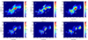 |
Fig. 2. Intensities of molecular lines in the PVDs along the major axis. The major axis of NGC 253 is marked by the solid black line in Fig. 1a, on which the black arrow shows the positive direction of position. (a) CO(1–0) PVD. The gray contours are drawn at [2, 10] K, and the blue contours are drawn at [20, 30] K. The white arrow points to the SW streamer and remains the same in the following panels. (b) 13CO(1–0) PVD. The gray contours are drawn at [0.3, 1.2, 2.0, 3.5] K. (c) HCN(1–0) PVD. The gray contours are drawn at [0.3, 1.2, 2.0, 3.5] K. (d) H13CN(1–0) PVD. The gray contours are drawn at [0.06, 0.25, 0.45] K and the blue contour is drawn at 0.62 K. (e) SiO(2–1) PVD. The gray contours are drawn at [0.06, 0.25, 0.45] K and the blue contour is drawn at 0.62 K. (f) CH3OH(2k–1k) PVD. The gray contours are drawn at [0.12, 0.50, 1.00, 1.50] K. |
The 13CO(1–0) PVD in Fig. 2b is less extended than the CO(1–0) and HCN(1–0) PVDs, but all have similar strong emission patterns. The H13CN(1–0), SiO(2–1), and CH3OH(2k–1k) PVDs in the second row of Fig. 3 are the least extended. For H13CN(1–0) and SiO(2–1) PVDs in Figs. 2d and 2e, the strong emission marked by the blue contours at 0.62 K is distributed in a few clumpy regions, among which the strongest two clumps are located near the base of the SW streamer (indicated by the white arrow). For the CH3OH(2k–1k) PVD in Fig. 2f, the strongest emission originates from the outskirts of the gas disk, which agrees with the integrated intensity map in Fig. 1f.
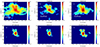 |
Fig. 3. Intensities of molecular lines in the PVDs along the SW slice. The SW slice is marked by the dashed black line in Fig. 1a, on which the black arrow shows the positive direction of the position. (a) CO(1–0) PVD. The gray contours are drawn at ∼[1.5, 10, 25] K. The dashed white profiles in panels a, b, and c outline the outflow in the SW streamer region. (b) 13CO(1–0) PVD. The gray contours are drawn at ∼[0.1, 0.9, 2.3] K. (c) HCN(1–0) PVD. The gray contours are drawn at ∼[0.1, 0.9, 3.2] K. (d) H13CN(1–0) PVD. The gray contours are drawn at ∼[0.03, 0.25] K. (e) SiO(2–1) PVD. The gray contours are drawn at ∼[0.03, 0.25] K. (f) CH3OH(2k–1k) PVD. The gray contours are drawn at ∼[0.03, 0.25] K. |
Figure 3 shows the intensities in the PVDs along a slice across the SW streamer (SW slice, dashed black line in Fig. 1a) with the systemic velocity reserved and distance taken to be zero in the slice center. The slice center is the same as in Fig. 1 from Walter et al. (2017), and the position angle of the slice equals 150°. In Fig. 3a, the CO(1–0) emission in the PVD is dominated by the disk component, and is extended toward the SW streamer in the region with D ∼ [ − 15, 0] arcsec and V ∼ 200 km s−1. Such an extension, outlined by the dashed white profiles, is consistent with Fig. 2 from Walter et al. (2017). The 13CO(1–0) and HCN(1–0) PVDs in Figs. 3b and 3c are less extended, but have similar patterns as the CO(1–0) PVD. The H13CN(1–0), SiO(2–1) and CH3OH(2k–1k) PVDs in the second row of Fig. 3 are the least extended, where the molecular emission only extends at the base of the SW streamer with D ∼ [ − 5, 0] arcsec and V ∼ 200 km s−1. The intensities of N2H+(1–0) in the PVDs along the major axis and along the SW slice are also checked, which show similar patterns to the H13CN(1–0) PVDs.
3.2. Gas kinematics
The CO(1–0) line is generally the best tracer of total molecular gas content thanks to its high abundance and low critical density for excitation. Figure 4 shows the kinematics of the molecular gas in NGC 253 traced with CO(1–0). There are two interesting kinematic features in Figs. 4a and 4b: (1) the velocity field showing gradients along both major and minor axes; (2) the blueshifted velocity and a high velocity dispersion in the SW streamer region.
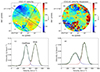 |
Fig. 4. Kinematic features of CO(1–0). (a) Velocity field of CO(1–0). The gray contours are the same as in Fig. 1a. The white contours mark the [175, 300] km s−1 velocity range with a step of 25 km s−1 in the central ∼100 pc. The solid white line shows the direction of the molecular bar. The solid and dashed black lines are the same as in Fig. 1a. The black arrow is the same as the white one in Fig. 1a, and indicates the same region in panel b and the following figures. (b) Velocity dispersion field of CO(1–0). The gray contours are the same as in panel a. The empty black ellipse outlines the high-velocity-dispersion region in the SW streamer region. The empty black circle inside the ellipse marks a beam-size region in the SW streamer region. (c) The averaged CO(1–0) spectrum from the empty black circle in panel b. The black profile shows the CO(1–0) line. The dashed blue profile shows the blueshifted Gaussian component. The dashed red profile shows the redshifted Gaussian component. The solid green profile is the superposition. (d) The averaged CO(1–0) spectrum from the empty black ellipse in panel b. The color codes are the same as in panel c. |
The white contours showing the velocity gradient in the center within a radius of ∼100 pc in Fig. 4a have the same pattern as the CO velocity field from Das et al. (2001) and Krieger et al. (2019). Their studies showed that the molecular bar shares the same direction as the stellar bar in the near-infrared band, and tilts ∼18° with respect to the major axis (Peng et al. 1996; Iodice et al. 2014). The direction of molecular and stellar bars is shown as a solid white line in Fig. 4a. There is a velocity gradient (white contours) in Fig. 4a in the direction of the molecular bar (solid white line), yet the ionized bar traced with the H92α recombination lines is almost parallel to the major axis (Cohen et al. 2020). Das et al. (2001) explained this phenomenon as different velocities of the gas moving in different bar orbits and suggested that the perturbation in the gas velocity field in NGC 253 is due to an accretion event that occurred ∼10 Myr ago.
The gas velocity in the SW streamer region (pointed out by the black arrow) is blueshifted (∼ 200 km s−1), as is shown in Fig. 4a, which means the outflowing gas is on the approaching side of NGC 253. The blueshifted outflow is visibly distinguishable from the redshifted (∼ 380 km s−1) disk rotation. Meanwhile, the other outflow streamers are indistinguishable in Fig. 4a, because they are fainter than SW streamer and/or located behind the galactic disk (Bolatto et al. 2013). In Fig. 4b, the gas in the SW streamer region presents a high velocity dispersion, which could be contributed by blueshifted outflow and redshifted rotation.
To compare the kinematics between the outflow and disk, we decomposed two components from the CO(1–0) spectra in the SW streamer region. From a circular region in the SW streamer region that has the same area as the beam size (the empty black circle in Fig. 4b), we extracted the averaged CO(1–0) spectrum, which is displayed by the solid black profile in Fig. 4c. The averaged CO(1–0) spectrum shows a double-peak structure, where we took the velocity ∼300 km s−1 as a reference velocity for the emission near the base of the SW streamer. Combining the velocity field of CO(1–0) in Fig. 4a, the blueshifted component relative to the reference velocity is emitted by the SW streamer, and the redshifted component is emitted by the gas disk. We also extracted the averaged CO(1–0) spectrum from a region with high velocity dispersion (high-σ) in the SW streamer region (the empty black ellipse in Fig. 4b), which is displayed by the solid black profile in Fig. 4d that also shows a double-peak structure. Using the Python-based tool curve_fit, we fit the CO(1–0) spectra in Figs. 4c and 4d with a double Gaussian function. The dashed blue profiles show the blueshifted Gaussian components, the dashed red profiles show the redshifted Gaussian components, and the solid green profiles show the superpositions. The velocity and full width at half maximum (FWHM) in the velocity space of each Gaussian component are listed in Table 1.
Results of double Gaussian fits for the CO(1–0) spectra.
We find that the blueshifted and redshifted components of the averaged CO(1–0) spectrum from the beam-size region (the empty black circle in Fig. 4b) have similar FWHMs in the velocity space (line widths). The redshifted component of the averaged CO(1–0) spectrum from the high-σ region (the empty black ellipse in Fig. 4b) has a similar FWHM to the components from the beam-size region, while the blueshifted component is ∼50% wider than the redshifted component. Moreover, there is a gradual velocity shift along the SW streamer in the CO(1–0) PVD outlined by the dashed white profiles in Fig. 3a. The velocity gradient inside the SW streamer could be evidence of an inside-out acceleration on the gas velocity; in other words, the gas inside the SW streamer is accelerated as it outflows. It could also be attributed to the ability of the fast ejecta to reach farther than the slow ejecta. Those two possibilities were also discussed in Walter et al. (2017). If we take the velocity center of the blueshifted component from the high-σ region (∼219.7 km s−1) to be the averaged velocity of the SW streamer, then the projected local velocity of the SW streamer equals ∼80 km s−1. Considering the inclination angle of the gas disk (∼78.5°) and the outflow being perpendicular to the disk, the deprojected local velocity of the SW streamer approaches ∼400 km s −1, which is comparable with the outflow velocity in the ionized gas phase (Westmoquette et al. 2011).
3.3. Optical depth
Figures 1a and 1b show the contours of CO(1–0) emission being more extended toward the SW streamer region than 13CO(1–0) emission, which could be a result of the different optical depths. Figure 5a shows the integrated intensity ratio map of CO/13CO(1–0) based on self-calibration, where we masked the regions with ratio S/N less than 3σ. The CO/13CO(1–0) ratio increases in the SW, southeastern (SE), and northwestern (NW) directions (named after Bolatto et al. 2013), pointed out by the black and gray arrows that are perpendicular to the gas disk (Fig. 5). The black contour with a CO/13CO(1–0) ratio of 15 defines the boundary between the outflow streamers and the disk. The CO/13CO(1–0) ratio further increases in part of the outflow region and is outlined by the blue contour at 21, where the CO/13CO(1–0) ratio is highest in the SW streamer region. CO is generally optically thick, while its isotopologue 13CO is optically thinner. The molecular gas in the CMZ of NGC 253 has shown a high kinetic temperature in previous studies (Paglione et al. 2004; Sakamoto et al. 2011), which weakens the fractionation effects on C-bearing species (Colzi et al. 2020). Moreover, 13C preferentially forms in the center, while C and 13C can be well mixed in the outflow region. The CO/13CO(1–0) ratio is expected to be similar to the C/13C isotope ratio in the optically thin limit, and decreases as the optical depth increases.
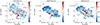 |
Fig. 5. Integrated intensity ratio maps. (a) Integrated intensity ratio map of CO/13CO(1–0). The ratios are taken in K km s−1 units, and remain the same in the following integrated intensity ratio plots. The black contour is drawn at 15 and the blue contour at 21. The gray arrows point to the outflow in the SE and NW directions. (b) Integrated intensity ratio map of HCN/13CO(1–0). The black contour is drawn at 1.4 and the blue contour at 2. (c) Integrated intensity ratio map of HCN/CO(1–0). The solid black line marks the major axis. The black contour is drawn at 0.09 and the blue contour at 0.15. The white contour is drawn at a CO/13CO(1–0) ratio of 15. The orange, purple, and yellow stars mark the positions at −1.5″, −4″, and −6.5″ offsets along the SW slice. The labels 3, 6, and 7 mark three GMCs. The gray arrows point to the outflow in the SE and NW directions. |
Martín et al. (2019) estimated a value of the isotopic ratio, C/13C ∼ 21 ± 6, via the integrated intensity ratio between C18O(1–0) and 13C18O(1–0). In Fig. 5a, the observed CO/13CO(1–0) ratio in the gas disk is lower than the C/13C ratio, which could be contributed by the optically thick CO emission in the disk. The CO/13CO(1–0) ratio in the SW, SE, and NW outflow regions approaches or exceeds the C/13C ratio, where the fluctuation in isotopic abundance is weak. Part of the outflow region (outlined by the blue contour at 21), including the SW streamer region, shows a CO/13CO(1–0) ratio consistent with the C/13C ratio. Except for NGC 253, Weiß et al. (2005) found the integrated intensity ratio CO/13CO(1–0) of the prominent molecular streamers to be comparable to that of the starburst disk in M82, which is different from the increasing CO/13CO(1–0) ratio toward the directions of outflow in NGC 253.
To decompose different velocity components, we plot in Figs. 6a and 6b the intensity ratio of CO/13CO(1–0) in the PVDs along the major axis and the SW slice, which are marked by the solid and dashed black lines in Fig. 1a. In Fig. 6a, the CO/13CO(1–0) ratio increases in the non-disk components and is highest on the blueshifted side, which implies a decrease in the optical depth of CO emission in the molecular gas on the approaching side of NGC 253. This phenomenon is more obvious in the PVD along the SW slice in Fig. 6b, where the CO/13CO(1–0) ratio is low along the gas disk and increases inside the SW streamer with D ∼ [ − 15, 0] arcsec and V ∼ 200 km s−1 outlined by the two dashed black profiles. Combining Figs. 5a, 6a, and 6b, we infer that the decrease in the optical depth of CO emission happens inside the molecular outflow including the SW streamer, which can be attributed to the gas velocity gradient inside the outflow.
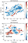 |
Fig. 6. Intensity ratio in the PVDs. (a) Intensity ratio of CO/13CO(1–0) in the PVD along the major axis. The black arrow points to the SW streamer and remains the same in subsequent figures. (b) Intensity ratio of CO/13CO(1–0) in the PVD along the SW slice. The dashed black profiles outline the outflow in the SW streamer region. |
Measuring the molecular mass outflow rate is important because it may indicate the rate at which the fuel for star formation is expelled, which may significantly suppress star formation activity. The optical depth of CO emission is a key factor in estimating the molecular mass outflow rate. Zschaechner et al. (2018) derived the optical depth with the integrated intensity ratio of CO(2–1)/CO(1–0) and suggested that the majority of the CO emission is optically thick in the outflow region of NGC 253. However, the 13C-bearing molecular species being optically thinner than the 12C-bearing ones implies that the CO/13CO(1–0) ratio is a more reliable indicator of the CO optical depth. Hence, the agreement between the CO/13CO(1–0) ratio (Fig. 5a) and the C/13C ratio (Martín et al. 2019) suggests that the CO emission in a considerable portion of the outflow region is optically thin in NGC 253. Such a phenomenon supports the estimation from Bolatto et al. (2013) of the total molecular mass outflow rate, ∼ 9 M⊙ yr−1, which is three times the star formation rate of ∼ 3 M⊙ yr−1 (Ott et al. 2005) in NGC 253.
HCN is one of the most abundant high dipole-moment molecules that trace dense gas. The permanent electric dipole-moment of HCN (μe ∼ 2.99 D) is much higher than CO (μe ∼ 0.11 D; Ebenstein & Muenter 1984; Goorvitch 1994), which makes the critical density of HCN three orders of magnitude higher than that of CO. Figure 5b shows the integrated intensity ratio map of HCN/13CO(1–0). The HCN/13CO(1–0) ratio is lowest in the gas disk, increases toward the outflow directions, and becomes highest in parts of the outflow region (outlined by the blue contour at a ratio of two) including the SW streamer region. Such a trend reminds us of the increasing CO/13CO(1–0) ratio in the outflow region with an increasing distance from the major axis in Fig. 5a. Given that HCN(1–0) emission is optically thick in the central ∼kpc region of NGC 253 (Meier et al. 2015), the increased line width attributed to the gas velocity gradient in the SW streamer region not only can decrease the optical depth of CO(1–0) emission tracing molecular gas, but can also decrease the optical depth of the HCN(1–0) emission tracing dense gas.
3.4. Dense gas fraction
The HCN/CO(1–0) ratio is widely used as an indicator of the fraction of dense gas, which is immediately responsible for the star formation inside galaxies (Gao & Solomon 2004a,b; Lada et al. 2012). Tanaka et al. (2024) presented non-LTE analyses with ALCHEMI data for the CMZ of NGC 253, and compared the dense gas fraction in this region with the center of the Milky Way. The difference turned out to be consistent with that in the HCN/CO(1–0) ratio between the CMZ of NGC 253 and the Galactic center, which confirms the HCN/CO(1–0) ratio as a good measurement of the mass fraction of the dense gas to the entire molecular gas.
Figure 5c shows the integrated intensity ratio map of HCN/CO(1–0). The HCN/CO(1–0) ratio is highest in three clumpy regions along the major axis (solid black line), which are marked by the blue contour at a ratio of 0.15. The physical sizes of the three regions in Fig. 5c are ≲100 pc, which fit the scales of giant molecular clouds (GMCs), and can be further resolved into star-forming clumps (∼10 pc; Ando et al. 2017). The positions of those GMCs are consistent with the observations in Leroy et al. (2015), which were numbered 3, 6, and 7. The bar of NGC 253 traced with ionized gas is also along the major axis (Das et al. 2001). The inflowing gas along the bar interacting with the gas in the disk can trigger star formation inside those GMCs. The existence of supernova remnants and the H II region in the inner 200 pc of NGC 253 was revealed about thirty years ago (Ulvestad & Antonucci 1997). The forming super star clusters and the winds from young clusters were detected at a high spatial resolution (Leroy et al. 2018; Levy et al. 2021, 2022). The GMCs 3, 6, and 7 in Fig. 5c are located at the base of outflow streamers outlined by the white contour, and the black contour at 0.09 is extended in the directions of outflow streamers. Given that the dynamical age of the SW streamer equaling ∼1 Myr is short (Walter et al. 2017), the star formation inside the GMCs can be the engine of the outflow streamers (Krieger et al. 2019).
Walter et al. (2017) measured the ratio of peak intensities between HCN(1–0) and CO(1–0), which equals ∼1/10 both in the SW streamer region and the starburst center of NGC 253. The orange, purple, and yellow stars in Fig. 5c mark the corresponding positions at −1.5″, −4″, and −6.5″ offsets from the slice center along the SW slice, following Walter et al. (2017). Based on the spatially resolved map, we can estimate the integrated intensity ratios at the three stars to be ∼0.19, 0.13, and 0.08. It is understandable that the dense gas fraction is highest inside the GMC and monotonously decreases away from the GMC.
Figures 7a and 7d show the intensity ratio of HCN/CO(1–0) in the PVDs along the major axis and the SW slice. In Fig. 7a, the HCN/CO(1–0) intensity ratio increases at the bottom of the PVD where the blueshifted non-disk component is located. In Fig. 7d, the HCN/CO(1–0) ratio is highest in the SW streamer region with D ∼ [ − 5, 0] arcsec and V ∼ 200 km s −1. Figures 4c and 4d show that the averaged projected velocity of the outflowing gas in the SW streamer region is around 200 km s −1. Hence, the HCN/CO(1–0) ratio increases in the gas at the base of the SW streamer that shares the same velocity as the molecular outflow. The HCN/CO(1–0) ratio in the extended streamer region with D ∼ [ − 15, −5] is moderate, as in the gas disk (Fig. 7d), which agrees with the tendency at −6.5″ offset in Fig. 7 from Walter et al. (2017).
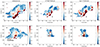 |
Fig. 7. First row: PVDs along the major axis. Second row: PVDs along the SW slice. (a,d) HCN/CO(1–0) ratio in PVDs. The dashed black profiles in panel d outline the outflow in the SW streamer region. (b,e) H13CN/13CO(1–0) ratio in PVDs. In panel e, the black ellipse named region A outlines the gas with D ∼ 0 arcsec and V ∼ 300 km s −1 and the black ellipse named region B outlines the gas with D ∼ [ − 5, 0] arcsec and V ∼ 200 km s−1; these are kept the same in subsequent figures. (c,f) N2H+/13CO(1–0) ratio in PVDs. |
It is possible to detect strong molecular emission at densities below the critical density. The effective excitation density is defined as the density at which the integrated intensity of a molecular line equals 1 K km s−1 with reasonable assumptions about the column density and kinetic temperature. Shirley (2015) calculated the optically thin critical densities and effective excitation densities at an assumed column density and kinetic temperature for the common dense gas tracers. The kinetic temperatures are assumed to be ∼100 K (Mangum et al. 2019) in the following comparisons of the effective excitation densities between different tracers. Shirley (2015) calculated the critical density and effective excitation density of HCN(1–0) at a column density of 1014 cm−2 to be 1.1 × 105 cm−3 and 1.7 × 103 cm−3, respectively.
To confirm the distribution of the dense gas in the CMZ of NGC 253, we turned to tracers of dense gas with a lower opacity. The critical density and effective excitation density of H13CN(1–0) at a column density of 1012.3 cm−2 equal 9.7 × 104 cm−3 and 6.5 × 104 cm−3, respectively. Even though the higher effective excitation density originates from a lower reference column density compared with that of HCN (Shirley 2015), H13CN(1–0) as an isotopologue can trace the dense gas with less limitation of optical depth. Figure 7b shows the intensity ratio of H13CN/13CO(1–0) in the PVD along the major axis, where the ratio also increases in the blueshifted non-disk component. Although the H13CN/13CO(1–0) ratio in the PVD along the SW slice in Fig. 7e is not as extended as HCN/CO(1–0), we still observe high ratios in two regions. One is the ellipse named region A with D ∼ 0 arcsec and V ∼ 300 km s −1 (reference velocity) that represents the gas inside GMC 3. The other is the ellipse named region B with D ∼ [ − 5, 0] arcsec and V ∼ 200 km s−1 (outflow velocity) that represents the gas at the base of the SW streamer.
The critical density and effective excitation density at a column density of 1013 cm−2 of another dense gas tracer, N2H+(1–0), equal 2 × 104 cm−3 and 2.6 × 103 cm−3, respectively. Even though the critical density of N2H+(1–0) is lower than HCN(1–0) and H13CN(1–0), Galactic parsec-scale observations show that the N2H+(1–0) emission is exclusively associated with rather dense gas (Kauffmann et al. 2017; Tafalla et al. 2021). The intensity ratio of N2H+/13CO(1–0) in the PVD along the major axis (Fig. 7c) has an accordant pattern with H13CN/13CO(1–0) PVD (Fig. 7b). In the PVD along the SW slice (Fig. 7f), the N2H+/13CO(1–0) ratio increases at the base of the SW streamer (region B). On the one hand, the increased patterns in Figs. 7d and 7f are highly consistent. Given that N2H+(1–0) is not safely optically thin and that the optical depths of HCN(1–0) and CO(1–0) can be different in the central region, the N2H+/13CO(1–0) and HCN/CO(1–0) ratios inside GMC 3 may be affected by optical depths. On the other hand, all three ratios in Figs. 7d, 7e, and 7f are higher in region B, which implies a negligible influence of optical depths at the base of the SW streamer, not to mention in the extended streamer region (Fig. 6b).
In summary, we find that the dense gas fraction is high inside GMC 3 (with reference velocity, region A) and at the base of the SW streamer (with outflow velocity, region B). The dense gas fraction in the extended streamer region (outlined by the dashed black profiles) is moderate in Fig. 7d and doesn’t show visible signs of accumulation of dense gas traced with HCN/CO(1–0). Combining the low optical depths of CO(1–0) and HCN(1–0) emission in the extended streamer region (Figs. 5a and 5b), we suggest the existence of a gas velocity gradient prevents the gas from accumulating inside the SW streamer of NGC 253.
3.5. Shock strength
Si-bearing material and solid-phase methanol are located in different parts of the dust grains. Silicon tends to reside in the core of grains and can be sputtered to the gas phase by fast shocks (vshock ≳ 15–20 km s−1, Kelly et al. 2017). Gas-phase silicon reacts with molecular oxygen or a hydroxyl radical and forms SiO (Schilke et al. 1997). On the other hand, solid-phase methanol is in the icy mantle of grains. Slow shocks (vshock ≲ 15–20 km s−1, Nesterenok 2022) are able to impact the icy mantle and inject gas-phase methanol into the ISM without destroying either the grain core or the methanol molecule (Millar et al. 1991; Charnley et al. 1995). Huang et al. (2023) studied the shock tracers SiO and HNCO with the ALCHEMI data and revealed a picture that most of the GMCs are subjected to shocks. They declared that HNCO may not be a unique tracer of slow shocks, while a high abundance of silicon in the gas phase can only be explained by fast shocks. In this section, we explore the methanol emission to verify the state of slow shocks, and inspect the relation between fast shocks traced by SiO emission and outflow streamers.
Figure 8a shows the integrated intensity ratio map of SiO(2–1)/CO(1–0). The three dense GMCs (labeled 3, 6, and 7, following Fig. 5c) also show an increased SiO(2–1)/CO(1–0) ratio that is marked by the blue contour at 0.01. Moreover, two SiO(2–1)/CO(1–0) ratio peaks appear around GMC 3 in Fig. 8a, with the second one consistent with the position of GMC 4 in Leroy et al. (2015). To examine the influence of optical depth, we also plot the integrated intensity ratio map of SiO(2–1)/13CO(1–0) in Fig. 8b. The increased SiO(2–1)/13CO(1–0) ratio exists in the four GMCs (marked by the blue contour at 0.1). The increased ratios in the GMCs imply the enhanced fast shocks there. The gray contour in Fig. 8b outlines the outflow streamers that originate from the four GMCs. Both the distributions of SiO(2–1)/CO(1–0) (marked by the black contour at 0.003) and SiO(2–1)/13CO(1–0) (marked by the black contour at 0.04) are extended toward the outflow streamers, which connect the fast shocks with the formation of the molecular outflow.
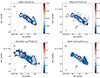 |
Fig. 8. Integrated intensity ratio maps. (a) Integrated intensity ratio map of SiO(2–1)/CO(1–0). The black contour is drawn at 0.003 and the blue contour at 0.01. The labels 3, 6, and 7 mark the three GMCs. (b) Integrated intensity ratio map of SiO(2–1)/13CO(1–0). The black contour is drawn at 0.04 and the blue contour at 0.1. The gray contour is drawn at a CO/13CO(1–0) ratio of 15. (c) Integrated intensity ratio map of CH3OH(2k–1k)/13CO(1–0). The black contour is drawn at 0.15 and the blue contour at 0.4. (d) Integrated intensity ratio map of SiO(2–1)/CH3OH(2k–1k). The black contour is drawn at 0.5 and the blue contour at 1. |
Figure 8c shows the integrated intensity ratio map of CH3OH(2k–1k)/13CO(1–0). The increased CH3OH(2k–1k)/13CO(1–0) ratio that is marked by the black contour at 0.15 is located on the outskirts of the gas disk. Locations with a high CH3OH(2k–1k)/13CO(1–0) ratio are similar to those with a high CH3OH(2k–1k) integrated intensity shown in Fig. 1f. Such a tendency is in agreement with HNCO 40, 4–30, 3 emission in Huang et al. (2023) that shows a high integrated intensity in the outermost CMZ of NGC 253. The strong methanol emission on the outskirts, with positions consistent with the methanol masers found by Gorski et al. (2017), implies the frequent occurrence of slow shocks. Meanwhile, the weak methanol emission in the center could be a result of the infrequent slow shocks, or the depletion of methanol molecules (Hartquist et al. 1995; Ellingsen et al. 2017) by fast shocks or photo-dissociation due to intense star formation (Humire et al. 2022). The non-co-spatial distributions of fast and slow shocks were also found in another nearby galaxy, NGC 1068 (Kelly et al. 2017), and imply that fast shocks do not necessarily occur with slow shocks. To obtain the relative strength between the fast and slow shocks, we plot the integrated intensity ratio map of SiO(2–1)/CH3OH(2k–1k) in Fig. 8d, where the central region turns out to be dominated by the fast shocks.
Figure 9 shows intensity ratios of the shock tracers in PVDs, where the top panels show the PVDs along the major axis and the bottom panels show the PVDs along the SW slice. The asymmetric and increased pattern (including regions A and B) of SiO(2–1)/13CO(1–0) ratio in PVDs (Figs. 9a and 9d) are highly similar to the H13CN/13CO(1–0) ratio in PVDs (Figs. 7b and 7e). We study in detail the correlation between the dense gas fraction and the strength of fast shocks in the next section. The increased intensity ratio of CH3OH(2k–1k)/13CO(1–0) on the outskirts of the gas disk in Fig. 9b is coherent with the distribution of the increased integrated intensity ratio in Fig. 8c. It is worth noting that a few red pixels located in region B of Fig. 9e indicate an enhancement of the slow shocks at the base of the SW streamer. In Figs. 9c and 9f, we plot the SiO(2–1)/CH3OH(2k–1k) ratio in PVDs. Region A in Fig. 9f is dominated by fast shocks, while the SiO(2–1)/CH3OH(2k–1k) ratio in region B is not so high as in region A. We infer that the fast shocks are triggered by the star formation inside GMC, which supports the second scenario for the origin of shocks in Huang et al. (2023). Meanwhile, the fast and slow shocks coexist in the SW streamer, and can further be related to the formation of the molecular outflow.
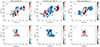 |
Fig. 9. First row: PVDs along the major axis. Second row: PVDs along the SW slice. (a,d) SiO(2–1)/13CO(1–0) ratio in PVDs. (b,e) CH3OH(2k–1k)/13CO(1–0) ratio in PVDs. (c,f) SiO(2–1)/CH3OH(2k–1k) ratio in PVDs. |
4. Formation of the molecular outflow
Walter et al. (2017) presented molecular spectra in the SW streamer region and quantified the relationship between the different molecular transitions, including CO(1–0) and HCN(1–0). Based on the data from the ALCHEMI survey, we can add several weaker molecular lines. In Fig. 10a, we plot orange, purple, and yellow stars, the same as in Fig. 5c, onto the self-calibrated integrated intensity ratio map of CO/13CO(1–0), where the increased ratio indicated by the red color represents the outflow region. The purple star is located at −4″ offset on the SW slice, following Walter et al. (2017). The molecular emission shown in Fig. 10b are averaged intensity profiles from a beam-size region centered on this purple star. The black profile shows the averaged intensity of the CO(1–0) spectrum (scaled down by a factor of 100), the red and gray profiles show the averaged intensities of HCN(1–0) and 13CO(1–0) spectra (scaled down by a factor of 10), and pink, orange, blue, and green profiles show the averaged intensities of H13CN(1–0), N2H+(1–0), SiO(2–1), and CH3OH(2k–1k) spectra, respectively.
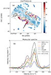 |
Fig. 10. Molecular spectra in the SW streamer region. (a) Integrated intensity ratio map of CO/13CO(1–0). The black contour is drawn at 15 and the blue contour at 21. The orange, purple, and yellow stars are the same as in Fig. 5c. (b) Averaged molecular spectra extracted from a beam-size region centered on the purple star in panel a. The color codes are labeled in the top left. The averaged intensity of the CO(1–0) line is scaled down by a factor of 100. The averaged intensities of 13CO(1–0) and HCN(1–0) lines are scaled down by a factor of 10. |
All the molecular lines in Fig. 10b show double-peak structures, which are in agreement with Fig. 7 from Walter et al. (2017) and CO(3–2) lines in Fig. 4 from Levy et al. (2022). The relatively weak blueshifted component is emitted by the SW streamer, and the relatively strong redshifted component is emitted by the gas disk. We used the Python-based tool curve_fit to conduct a double Gaussian fit on each molecular line. The peak intensities, together with errors from the Gaussian fit of the streamer and disk components for each molecular line, are listed in the second and third columns of Table 2, and the corresponding line name is listed in the first column. Although the streamer component is weak in the SiO(2–1) line, it exists in all the molecular lines that are extracted from the beam-size region (purple star in Fig. 10a) in the SW streamer.
As was described in the introduction, three main formation scenarios have previously been proposed for the molecular outflow. One is molecular outflow directly driven by radiation and/or pressure, one is a molecular cloud entrained by hot wind, and the other is molecular outflow in situ forming from the hot wind. The last scenario assumes the cooling timescale to be shorter than the dynamical timescale (Efstathiou 2000; Silich et al. 2003). Walter et al. (2017) estimated that the molecular gas inside the SW streamer of NGC 253 was ejected from the disk ∼1 Myr ago, which is too short to create new CO molecules that can emit (Clark et al. 2012). Moreover, the phenomenon that all the molecular lines in Table 2 show streamer features indicates that the SW streamer starts as dense, shocked, and chemically rich outflowing gas. The existence of dense gas tracers, for example HCN, H13CN, and N2H+, inside the outflow further excludes the possibility of in situ formation. However, it is still difficult to distinguish whether the outflowing molecular gas is directly driven by radiation or pressure, or whether it is entrained by the hot wind.
Figure 11a shows the integrated intensity ratio map of H13CN/13CO(1–0), where the GMCs have the highest ratios marked by the blue contour at 0.12, and the black contour at 0.06 is extended toward the outflow streamers. Such increased patterns are similar to that of SiO(2–1)/13CO(1–0) in Fig. 8b. Moreover, the increased H13CN/13CO(1–0) and SiO(2–1)/13CO(1–0) ratios in PVDs in Figs. 7 and 9 also share similar patterns. The consistency in the enhanced emissions of H13CN(1–0) and SiO(2–1) implies a positive correlation between the dense gas fraction and the strength of fast shocks in NGC 253. We regridded the H13CN(1–0), SiO(2–1) and 13CO(1–0) data cubes to a 1.6″ beam-size to avoid oversampling, then statistically quantified the linear relationship between H13CN/13CO(1–0) and SiO(2–1)/13CO(1–0).
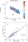 |
Fig. 11. Correlation between the dense gas fraction and the strength of fast shocks. (a) Integrated intensity ratio map of H13CN/13CO(1–0). The black contour is drawn at 0.06 and the blue contour at 0.12. The labels 3, 6, and 7 mark the same GMCs as in Fig. 5c. (b) Correlation between H13CN/13CO(1–0) and SiO(2–1)/13CO(1–0). The blue points mark the ratios from pixels with a spatial resolution equaling the beam size. The solid gray line shows the result of a linear fit to the blue points. |
The blue points in Fig. 11b show the H13CN/13CO(1–0) and SiO(2–1)/13CO(1–0) ratios in each beam-size region from Figs. 8b and 11a. To check the linear relationship between the two ratios, which is visibly tight, we calculated the Pearson correlation coefficient using the Python-based package pearsonr. The correlation coefficient (r) equals 0.85, which reveals a tight positive correlation between the H13CN/13CO(1–0) and SiO(2–1)/13CO(1–0) ratios. We performed a linear fit for the dataset, which is shown by the solid gray line in Fig. 11b. We also calculated the Pearson correlation coefficient between H13CN(1–0) and SiO(2–1) integrated intensities, which approaches 0.96 and reveals a tight correlation between the intensities of two lines. Therefore, the correlation between H13CN/13CO(1–0) and SiO(2–1)/13CO(1–0) ratios is real and not a result of the common denominator. Meanwhile, we keep in mind that the high critical densities of H13CN(1–0) and SiO(2–1) may contribute to the tight positive correlation between the two ratios. Theoretically, the star formation that happens in the region with a high dense gas fraction can trigger fast shocks. Combining the similar extensions of the SiO(2–1) and H13CN(1–0) emissions toward the outflow in Figs. 8b and 11a, the star formation inside the GMCs can trigger fast shocks and contribute to the formation of the molecular outflow in NGC 253.
The difference between the tracers of dense gas and shocks presents when we further analyze the molecular spectra in Fig. 10b. Given that all the lines show double-peak structures, we can distinguish the contributions of steamer and disk via the double Gaussian fits. In the last column of Table 2, we list the streamer-to-disk peak intensity ratios (streamer-to-disk ratios for short) together with errors for different molecular lines. Each ratio was calculated by dividing the peak intensity of the streamer component by that of the disk component.
The streamer-to-disk ratio of CO(1–0) is higher than its isotopologue 13CO(1–0), which can be explained by the lower-opacity environment inside the SW streamer than in the gas disk for CO emission, as is discussed in Sect. 3.3. It is interesting to find that all the dense gas tracers (marked by the star symbols in the first column of Table 2) have higher streamer-to-disk ratios than the others. The optical depth decreasing inside the SW streamer for HCN emission can explain the highest streamer-to-disk ratio of HCN(1–0) among the dense gas tracers. In addition, the SiO(2–1) and methanol, as the tracers of fast and slow shocks, respectively, have similar streamer-to-disk ratios to 13CO(1–0). It seems that the enhancement of the dense gas fraction is stronger in the SW streamer than in the gas disk, while the shock strength is equivalently enhanced in the SW streamer and the gas disk. More detailed clues are needed to explain such a difference.
We suggest the physical pictures that are related to the SW streamer in NGC 253 as follows: (i) The GMCs (Fig. 5c) in the direction of the major axis are related to the gas accretion along the bar structure that provides further material for the star formation. Meanwhile, the star formation inside the GMCs that are located at the base of the outflow streamers contributes to driving the molecular outflow, which is in agreement with the model presented by Levy et al. (2022). (ii) There can be intense star formation inside the GMCs also presenting as a higher dense gas fraction, and this results in an enhanced shock strength at the base of the outflow (Figs. 7 and 9) including the SW streamer. (iii) The optical depths of CO and HCN emission decrease in the SW streamer (Figs. 5a and 5b), and the dense gas is diluted in the extended SW streamer region (Fig. 7d), which can be attributed to the gas velocity gradient inside the molecular outflow.
5. Summary
In this work, we analyze data from the ALCHEMI survey and study the physical properties of the molecular outflow in the starburst galaxy NGC 253.
-
(1)
The emission of CO(1–0), 13CO(1–0), HCN(1–0), H13CN(1–0), N2H+(1–0) and CH3OH(2k–1k) is extended toward the SW streamer. The CO(1–0) and HCN(1–0) emission is the most extended, which can be attributed to the optically thick environments in the gas disk and decreased optical depths toward the SW streamer.
-
(2)
The molecular outflow in the SW streamer region is blueshifted with a deprojected local velocity of ∼400 km s−1, which is consistent with previous studies. The wider blueshifted component than the disk component suggests an inside-out acceleration of molecular outflow or the fast ejecta getting farther away than the slow ejecta. All the molecular spectra from the SW streamer region show double-peak structures, which indicate that the SW streamer starts as dense, shocked, and chemically rich outflowing gas, rather than in situ formation from hot wind.
-
(3)
The integrated intensity ratio maps of CO/13CO(1–0) and HCN/13CO(1–0) show similar patterns. Both are lowest in the gas disk, increase in outflow directions that are perpendicular to the gas disk, and become highest in the SW streamer region. Combining the isotopic ratio of C/13C from a previous study, we suggest that the CO(1–0) emission is optically thin in the SW streamer region, which may be a result of the gas velocity gradient.
-
(4)
Three GMCs are present in the integrated intensity ratio map of HCN/CO(1–0), which are aligned with the direction of the major axis and could be caused by the gas accretion along the bar structure. Those GMCs are located at the base of the outflow streamers including the SW streamer, where the star formation could drive molecular outflow. The HCN/CO(1–0), H13CN/13CO(1–0) and N2H+/13CO(1–0) intensity ratios in PVDs show a high dense gas fraction at the base of the SW streamer. The HCN/CO(1–0) intensity ratio in PVDs suggests a moderate dense gas fraction in the extended streamer region without visible signs of the accumulation of dense gas, which may also be a result of the gas velocity gradient.
-
(5)
The SiO(2–1)/CO(1–0) and SiO(2–1)/13CO(1–0) integrated intensity ratios show enhanced fast shocks in the GMCs. The SiO(2–1)/13CO(1–0) and CH3OH(2k–1k)/13CO(1–0) intensity ratios in PVDs indicate that fast shocks can be triggered by the star formation inside GMCs, while fast and slow shocks coexist at the base of the SW streamer and could be related to the formation of molecular outflow.
-
(6)
There is a tight positive correlation between the dense gas fraction traced with H13CN/13CO(1–0) and the strength of fast shocks traced with SiO(2–1)/13CO(1–0). The dense gas fraction is high in GMCs, where the star formation can trigger fast shocks and contribute to the formation of molecular outflow. One difference is that the enhancement of the dense gas fraction is more tightly related to the SW streamer than the gas disk, while the shock strength is equivalently enhanced in the SW streamer and the gas disk.
Acknowledgments
This paper makes use of the following ALMA data: ADS/JAO.ALMA#2017.1.00161.L. ALMA is a partnership of ESO (representing its member states), NSF (USA) and NINS (Japan), together with NRC (Canada), MOST and ASIAA (Taiwan), and KASI (Republic of Korea), in cooperation with the Republic of Chile. The Joint ALMA Observatory is operated by ESO, AUI/NRAO and NAOJ. This work was supported by JSPS KAKENHI Grant Number JP17H06130 and the NAOJ ALMA Scientific Research Grant Number 2017-06B. M.B. acknowledges support from the National Natural Science Foundation of China (No. 12303009) and the China Scholarship Council (No. 202006860042). N.H. acknowledges support from JSPS KAKENHI Grant Number JP21K03634. F.E. is financially supported by JSPS KAKENHI Grant Numbers JP17K14259 and JP20H00172. L.C. acknowledges financial support through the Spanish grant PID2019-105552RB-C41 funded by MCIN/AEI/10.13039/501100011033. V.M.R. has received support from the project RYC2020-029387-I funded by MCIN/AEI/10.13039/501100011033. S.V., M.B., and K-Y. Huang acknowledge support from the European Research Council (ERC) under the European Union’s Horizon 2020 research and innovation programme MOPPEX 833460. L.C. and V.M.R. acknowledge funding from grants No. PID2019-105552RB-C41 and PID2022-136814NB-I00 by the Spanish Ministry of Science, Innovation and Universities/State Agency of Research MICIU/AEI/10.13039/501100011033 and by ERDF, UE. V.M.R. also acknowledges support from the grant number RYC2020-029387-I funded by MICIU/AEI/10.13039/501100011033 and by ESF, Investing in your future, and from the Consejo Superior de Investigaciones Científicas (CSIC) and the Centro de Astrobiología (CAB) through the project 20225AT015 (Proyectos intramurales especiales del CSIC). M.B. acknowledges Prof. Yu Gao for his remarkable discovery of the HCN J = 1–0 as an indicator of dense molecular gas, as well as for his gentle clarification to her regarding the ALMA instrument in 2018.
References
- Aalto, S. 2015, Revolution in Astronomy with ALMA: The Third Year, 499, 85 [NASA ADS] [Google Scholar]
- ALMA Partnership (Fomalont, E. B., et al.) 2015, ApJ, 808, L1 [Google Scholar]
- Aladro, R., Martín, S., Riquelme, D., et al. 2015, A&A, 579, A101 [NASA ADS] [CrossRef] [EDP Sciences] [Google Scholar]
- Ando, R., Nakanishi, K., Kohno, K., et al. 2017, ApJ, 849, 81 [CrossRef] [Google Scholar]
- Banda-Barragán, W. E., Zertuche, F. J., Federrath, C., et al. 2019, MNRAS, 486, 4526 [CrossRef] [Google Scholar]
- Barnes, A. T., Kauffmann, J., Bigiel, F., et al. 2020, MNRAS, 497, 1972 [NASA ADS] [CrossRef] [Google Scholar]
- Behrens, E., Mangum, J. G., Holdship, J., et al. 2022, ApJ, 939, 119 [NASA ADS] [CrossRef] [Google Scholar]
- Bendo, G. J., Beswick, R. J., D’Cruze, M. J., et al. 2015, MNRAS, 450, L80 [NASA ADS] [CrossRef] [Google Scholar]
- Bolatto, A. D., Warren, S. R., Leroy, A. K., et al. 2013, Nature, 499, 450 [Google Scholar]
- Brunthaler, A., Castangia, P., Tarchi, A., et al. 2009, A&A, 497, 103 [NASA ADS] [CrossRef] [EDP Sciences] [Google Scholar]
- CASA Team (Bean, B., et al.) 2022, PASP, 134, 114501 [NASA ADS] [CrossRef] [Google Scholar]
- Charnley, S. B., Kress, M. E., Tielens, A. G. G. M., et al. 1995, ApJ, 448, 232 [NASA ADS] [CrossRef] [Google Scholar]
- Clark, P. C., Glover, S. C. O., Klessen, R. S., et al. 2012, MNRAS, 424, 2599 [CrossRef] [Google Scholar]
- Cohen, D. P., Turner, J. L., & Consiglio, S. M. 2020, MNRAS, 493, 627 [NASA ADS] [CrossRef] [Google Scholar]
- Colzi, L., Sipilä, O., Roueff, E., et al. 2020, A&A, 640, A51 [NASA ADS] [CrossRef] [EDP Sciences] [Google Scholar]
- Das, M., Anantharamaiah, K. R., & Yun, M. S. 2001, ApJ, 549, 896 [NASA ADS] [CrossRef] [Google Scholar]
- Ebenstein, W. L., & Muenter, J. S. 1984, J. Chem. Phys., 80, 3989 [Google Scholar]
- Efstathiou, G. 2000, MNRAS, 317, 697 [NASA ADS] [CrossRef] [Google Scholar]
- Ellingsen, S. P., Chen, X., Breen, S. L., et al. 2017, MNRAS, 472, 604 [NASA ADS] [CrossRef] [Google Scholar]
- Engelbracht, C. W., Rieke, M. J., Rieke, G. H., et al. 1998, ApJ, 505, 639 [NASA ADS] [CrossRef] [Google Scholar]
- Fielding, D. B., & Bryan, G. L. 2022, ApJ, 924, 82 [NASA ADS] [CrossRef] [Google Scholar]
- Gao, Y., & Solomon, P. M. 2004a, ApJ, 606, 271 [NASA ADS] [CrossRef] [Google Scholar]
- Gao, Y., & Solomon, P. M. 2004b, ApJS, 152, 63 [Google Scholar]
- García-Burillo, S., Usero, A., Fuente, A., et al. 2010, A&A, 519, A2 [NASA ADS] [CrossRef] [EDP Sciences] [Google Scholar]
- Goorvitch, D. 1994, ApJS, 95, 535 [NASA ADS] [CrossRef] [Google Scholar]
- Gorski, M., Ott, J., Rand, R., et al. 2017, ApJ, 842, 124 [CrossRef] [Google Scholar]
- Greisen, E. W. 2003, Inf. Handling Astron. - Hist. Vistas, 285, 109 [NASA ADS] [CrossRef] [Google Scholar]
- Ginsburg, A., Robitaille, T., & Beaumont, C. 2016, Astrophysics Source Code Library [record ascl:1608.010] [Google Scholar]
- Haasler, D., Rivilla, V. M., Martín, S., et al. 2022, A&A, 659, A158 [CrossRef] [EDP Sciences] [Google Scholar]
- Harada, N., Martín, S., Mangum, J. G., et al. 2021, ApJ, 923, 24 [NASA ADS] [CrossRef] [Google Scholar]
- Harada, N., Martín, S., Mangum, J. G., et al. 2022, ApJ, 938, 80 [NASA ADS] [CrossRef] [Google Scholar]
- Hartquist, T. W., Menten, K. M., Lepp, S., et al. 1995, MNRAS, 272, 184 [NASA ADS] [CrossRef] [Google Scholar]
- Heckman, T. M., Lehnert, M. D., Strickland, D. K., et al. 2000, ApJS, 129, 493 [NASA ADS] [CrossRef] [Google Scholar]
- Heesen, V., Beck, R., Krause, M., et al. 2011, A&A, 535, A79 [NASA ADS] [CrossRef] [EDP Sciences] [Google Scholar]
- Hollenbach, D., & Salpeter, E. E. 1971, ApJ, 163, 155 [NASA ADS] [CrossRef] [Google Scholar]
- Huang, K.-Y., Viti, S., Holdship, J., et al. 2023, A&A, 675, A151 [NASA ADS] [CrossRef] [EDP Sciences] [Google Scholar]
- Holdship, J., Viti, S., Martín, S., et al. 2021, A&A, 654, A55 [NASA ADS] [CrossRef] [EDP Sciences] [Google Scholar]
- Holdship, J., Mangum, J. G., Viti, S., et al. 2022, ApJ, 931, 89 [NASA ADS] [CrossRef] [Google Scholar]
- Humire, P. K., Henkel, C., Hernández-Gómez, A., et al. 2022, A&A, 663, A33 [NASA ADS] [CrossRef] [EDP Sciences] [Google Scholar]
- Iodice, E., Arnaboldi, M., Rejkuba, M., et al. 2014, A&A, 567, A86 [NASA ADS] [CrossRef] [EDP Sciences] [Google Scholar]
- Israel, F. P. 2020, A&A, 635, A131 [NASA ADS] [CrossRef] [EDP Sciences] [Google Scholar]
- Kauffmann, J., Goldsmith, P. F., Melnick, G., et al. 2017, A&A, 605, L5 [NASA ADS] [CrossRef] [EDP Sciences] [Google Scholar]
- Kelly, G., Viti, S., García-Burillo, S., et al. 2017, A&A, 597, A11 [NASA ADS] [CrossRef] [EDP Sciences] [Google Scholar]
- Klein, R. I., McKee, C. F., & Colella, P. 1994, ApJ, 420, 213 [Google Scholar]
- Kormendy, J., & Ho, L. C. 2013, ARA&A, 51, 511 [Google Scholar]
- Krieger, N., Bolatto, A. D., Walter, F., et al. 2019, ApJ, 881, 43 [NASA ADS] [CrossRef] [Google Scholar]
- Lada, C. J., Forbrich, J., Lombardi, M., et al. 2012, ApJ, 745, 190 [NASA ADS] [CrossRef] [Google Scholar]
- Le Bourlot, J., Le Petit, F., Pinto, C., et al. 2012, A&A, 541, A76 [NASA ADS] [CrossRef] [EDP Sciences] [Google Scholar]
- Lefèvre, C., Kramer, C., Neri, R., Berta, S., & Schuster, K. 2020, EPJ Web Conf., 228, 00014 [CrossRef] [EDP Sciences] [Google Scholar]
- Leroy, A. K., Bolatto, A. D., Ostriker, E. C., et al. 2015, ApJ, 801, 25 [NASA ADS] [CrossRef] [Google Scholar]
- Leroy, A. K., Bolatto, A. D., Ostriker, E. C., et al. 2018, ApJ, 869, 126 [NASA ADS] [CrossRef] [Google Scholar]
- Lopez, S., Lopez, L. A., Nguyen, D. D., et al. 2023, ApJ, 942, 108 [NASA ADS] [CrossRef] [Google Scholar]
- Levy, R. C., Bolatto, A. D., Leroy, A. K., et al. 2021, ApJ, 912, 4 [NASA ADS] [CrossRef] [Google Scholar]
- Levy, R. C., Bolatto, A. D., Leroy, A. K., et al. 2022, ApJ, 935, 19 [NASA ADS] [CrossRef] [Google Scholar]
- Mangum, J. G., Ginsburg, A. G., Henkel, C., et al. 2019, ApJ, 871, 170 [NASA ADS] [CrossRef] [Google Scholar]
- Martín, S., Muller, S., Henkel, C., et al. 2019, A&A, 624, A125 [NASA ADS] [CrossRef] [EDP Sciences] [Google Scholar]
- Martín, S., Mangum, J. G., Harada, N., et al. 2021, A&A, 656, A46 [NASA ADS] [CrossRef] [EDP Sciences] [Google Scholar]
- Meier, D. S., Walter, F., Bolatto, A. D., et al. 2015, ApJ, 801, 63 [NASA ADS] [CrossRef] [Google Scholar]
- Millar, T. J., Herbst, E., & Charnley, S. B. 1991, ApJ, 369, 147 [Google Scholar]
- Murray, N., Ménard, B., & Thompson, T. A. 2011, ApJ, 735, 66 [NASA ADS] [CrossRef] [Google Scholar]
- Nesterenok, A. V. 2022, MNRAS, 509, 4555 [Google Scholar]
- Orlando, S., Peres, G., Reale, F., et al. 2005, A&A, 444, 505 [NASA ADS] [CrossRef] [EDP Sciences] [Google Scholar]
- Ott, J., Weiss, A., Henkel, C., et al. 2005, ApJ, 629, 767 [NASA ADS] [CrossRef] [Google Scholar]
- Paglione, T. A. D., Yam, O., Tosaki, T., et al. 2004, ApJ, 611, 835 [NASA ADS] [CrossRef] [Google Scholar]
- Pantaleone, S., Enrique-Romero, J., Ceccarelli, C., et al. 2021, ApJ, 917, 49 [CrossRef] [Google Scholar]
- Peng, R., Zhou, S., Whiteoak, J. B., et al. 1996, ApJ, 470, 821 [NASA ADS] [CrossRef] [Google Scholar]
- Pietsch, W., Vogler, A., Klein, U., et al. 2000, A&A, 360, 24 [NASA ADS] [Google Scholar]
- Rekola, R., Richer, M. G., McCall, M. L., et al. 2005, MNRAS, 361, 330 [NASA ADS] [CrossRef] [Google Scholar]
- Rieke, G. H., Lebofsky, M. J., Thompson, R. I., et al. 1980, ApJ, 238, 24 [NASA ADS] [CrossRef] [Google Scholar]
- Sakamoto, K., Mao, R.-Q., Matsushita, S., et al. 2011, ApJ, 735, 19 [CrossRef] [Google Scholar]
- Sánchez-Monge, Á., Schilke, P., Ginsburg, A., et al. 2018, A&A, 609, A101 [NASA ADS] [CrossRef] [EDP Sciences] [Google Scholar]
- Schilke, P., Walmsley, C. M., Pineau des Forets, G., et al. 1997, A&A, 321, 293 [Google Scholar]
- Shirley, Y. L. 2015, PASP, 127, 299 [Google Scholar]
- Silich, S., Tenorio-Tagle, G., & Muñoz-Tuñón, C. 2003, ApJ, 590, 791 [NASA ADS] [CrossRef] [Google Scholar]
- Socrates, A., Davis, S. W., & Ramirez-Ruiz, E. 2008, ApJ, 687, 202 [NASA ADS] [CrossRef] [Google Scholar]
- Spilker, J. S., Bezanson, R., Weiner, B. J., et al. 2019, ApJ, 883, 81 [NASA ADS] [CrossRef] [Google Scholar]
- Strickland, D. K., Heckman, T. M., Weaver, K. A., et al. 2000, AJ, 120, 2965 [NASA ADS] [CrossRef] [Google Scholar]
- Strickland, D. K., Heckman, T. M., Weaver, K. A., et al. 2002, ApJ, 568, 689 [NASA ADS] [CrossRef] [Google Scholar]
- Sturm, E., González-Alfonso, E., Veilleux, S., et al. 2011, ApJ, 733, L16 [NASA ADS] [CrossRef] [Google Scholar]
- Tacchella, S., Carollo, C. M., Renzini, A., et al. 2015, Science, 348, 314 [NASA ADS] [CrossRef] [Google Scholar]
- Tacchella, S., Dekel, A., Carollo, C. M., et al. 2016, MNRAS, 458, 242 [NASA ADS] [CrossRef] [Google Scholar]
- Tafalla, M., Usero, A., & Hacar, A. 2021, A&A, 646, A97 [NASA ADS] [CrossRef] [EDP Sciences] [Google Scholar]
- Takano, S., Nakajima, T., & Kohno, K. 2019, PASJ, 71, S20 [Google Scholar]
- Tanaka, K., Mangum, J. G., Viti, S., et al. 2024, ApJ, 961, 18 [NASA ADS] [CrossRef] [Google Scholar]
- Turner, B. E. 1985, ApJ, 299, 312 [NASA ADS] [CrossRef] [Google Scholar]
- Uhlig, M., Pfrommer, C., Sharma, M., et al. 2012, MNRAS, 423, 2374 [CrossRef] [Google Scholar]
- Ulvestad, J. S., & Antonucci, R. R. J. 1997, ApJ, 488, 621 [NASA ADS] [CrossRef] [Google Scholar]
- Veilleux, S., Cecil, G., & Bland-Hawthorn, J. 2005, ARA&A, 43, 769 [NASA ADS] [CrossRef] [Google Scholar]
- Veilleux, S., Kim, D.-C., Rupke, D. S. N., et al. 2009, ApJ, 701, 587 [NASA ADS] [CrossRef] [Google Scholar]
- Veilleux, S., Maiolino, R., Bolatto, A. D., et al. 2020, A&A Rev., 28, 2 [NASA ADS] [CrossRef] [Google Scholar]
- Walter, F., Bolatto, A. D., Leroy, A. K., et al. 2017, ApJ, 835, 265 [NASA ADS] [CrossRef] [Google Scholar]
- Weiß, A., Walter, F., & Scoville, N. Z. 2005, A&A, 438, 533 [NASA ADS] [CrossRef] [EDP Sciences] [Google Scholar]
- Westmoquette, M. S., Smith, L. J., & Gallagher, J. S. 2011, MNRAS, 414, 3719 [NASA ADS] [CrossRef] [Google Scholar]
- Zschaechner, L. K., Bolatto, A. D., Walter, F., et al. 2018, ApJ, 867, 111 [NASA ADS] [CrossRef] [Google Scholar]
All Tables
All Figures
|
Fig. 1. Integrated intensity maps of the transitions used in this work. (a) Integrated intensity map of CO(1–0). The white contour is drawn at 180 K km s−1, the gray contours are drawn at [360, 720, 1440, 2880] K km s−1, and the blue contour is drawn at 4300 K km s−1. The horizontal lines in different colors inside the color bar mark the values of corresponding contours, and remain the same in the following figures. The solid black line marks the major axis, and the dashed black line marks the slice across the SW streamer, on which the black arrows show the positive directions of the PVDs in the following figures. The white arrow points to the SW streamer and remains the same in subsequent panels. The black cross marks the phase center of the observation and remains the same in subsequent figures. The beam size of 1.6″ is shown as an empty black circle in the bottom-left corner of each panel and remains the same in subsequent figures. (b) Integrated intensity map of 13CO(1–0). The gray contours are drawn at [12, 40, 120, 230, 460] K km s−1. (c) Integrated intensity map of HCN(1–0). The gray contours are drawn at [12, 40, 120, 300, 670] K km s−1. (d) Integrated intensity map of H13CN(1–0). The gray contours are drawn at [2, 8, 20, 50, 100] K km s−1. (e) Integrated intensity map of N2H+(1–0). The gray contours are drawn at [5, 20, 50, 100, 200] K km s−1. (f) Integrated intensity map of CH3OH(2k–1k). The gray contours are drawn at [5, 20, 50, 100, 200] K km s−1. |
| In the text | |
|
Fig. 2. Intensities of molecular lines in the PVDs along the major axis. The major axis of NGC 253 is marked by the solid black line in Fig. 1a, on which the black arrow shows the positive direction of position. (a) CO(1–0) PVD. The gray contours are drawn at [2, 10] K, and the blue contours are drawn at [20, 30] K. The white arrow points to the SW streamer and remains the same in the following panels. (b) 13CO(1–0) PVD. The gray contours are drawn at [0.3, 1.2, 2.0, 3.5] K. (c) HCN(1–0) PVD. The gray contours are drawn at [0.3, 1.2, 2.0, 3.5] K. (d) H13CN(1–0) PVD. The gray contours are drawn at [0.06, 0.25, 0.45] K and the blue contour is drawn at 0.62 K. (e) SiO(2–1) PVD. The gray contours are drawn at [0.06, 0.25, 0.45] K and the blue contour is drawn at 0.62 K. (f) CH3OH(2k–1k) PVD. The gray contours are drawn at [0.12, 0.50, 1.00, 1.50] K. |
| In the text | |
|
Fig. 3. Intensities of molecular lines in the PVDs along the SW slice. The SW slice is marked by the dashed black line in Fig. 1a, on which the black arrow shows the positive direction of the position. (a) CO(1–0) PVD. The gray contours are drawn at ∼[1.5, 10, 25] K. The dashed white profiles in panels a, b, and c outline the outflow in the SW streamer region. (b) 13CO(1–0) PVD. The gray contours are drawn at ∼[0.1, 0.9, 2.3] K. (c) HCN(1–0) PVD. The gray contours are drawn at ∼[0.1, 0.9, 3.2] K. (d) H13CN(1–0) PVD. The gray contours are drawn at ∼[0.03, 0.25] K. (e) SiO(2–1) PVD. The gray contours are drawn at ∼[0.03, 0.25] K. (f) CH3OH(2k–1k) PVD. The gray contours are drawn at ∼[0.03, 0.25] K. |
| In the text | |
|
Fig. 4. Kinematic features of CO(1–0). (a) Velocity field of CO(1–0). The gray contours are the same as in Fig. 1a. The white contours mark the [175, 300] km s−1 velocity range with a step of 25 km s−1 in the central ∼100 pc. The solid white line shows the direction of the molecular bar. The solid and dashed black lines are the same as in Fig. 1a. The black arrow is the same as the white one in Fig. 1a, and indicates the same region in panel b and the following figures. (b) Velocity dispersion field of CO(1–0). The gray contours are the same as in panel a. The empty black ellipse outlines the high-velocity-dispersion region in the SW streamer region. The empty black circle inside the ellipse marks a beam-size region in the SW streamer region. (c) The averaged CO(1–0) spectrum from the empty black circle in panel b. The black profile shows the CO(1–0) line. The dashed blue profile shows the blueshifted Gaussian component. The dashed red profile shows the redshifted Gaussian component. The solid green profile is the superposition. (d) The averaged CO(1–0) spectrum from the empty black ellipse in panel b. The color codes are the same as in panel c. |
| In the text | |
|
Fig. 5. Integrated intensity ratio maps. (a) Integrated intensity ratio map of CO/13CO(1–0). The ratios are taken in K km s−1 units, and remain the same in the following integrated intensity ratio plots. The black contour is drawn at 15 and the blue contour at 21. The gray arrows point to the outflow in the SE and NW directions. (b) Integrated intensity ratio map of HCN/13CO(1–0). The black contour is drawn at 1.4 and the blue contour at 2. (c) Integrated intensity ratio map of HCN/CO(1–0). The solid black line marks the major axis. The black contour is drawn at 0.09 and the blue contour at 0.15. The white contour is drawn at a CO/13CO(1–0) ratio of 15. The orange, purple, and yellow stars mark the positions at −1.5″, −4″, and −6.5″ offsets along the SW slice. The labels 3, 6, and 7 mark three GMCs. The gray arrows point to the outflow in the SE and NW directions. |
| In the text | |
|
Fig. 6. Intensity ratio in the PVDs. (a) Intensity ratio of CO/13CO(1–0) in the PVD along the major axis. The black arrow points to the SW streamer and remains the same in subsequent figures. (b) Intensity ratio of CO/13CO(1–0) in the PVD along the SW slice. The dashed black profiles outline the outflow in the SW streamer region. |
| In the text | |
|
Fig. 7. First row: PVDs along the major axis. Second row: PVDs along the SW slice. (a,d) HCN/CO(1–0) ratio in PVDs. The dashed black profiles in panel d outline the outflow in the SW streamer region. (b,e) H13CN/13CO(1–0) ratio in PVDs. In panel e, the black ellipse named region A outlines the gas with D ∼ 0 arcsec and V ∼ 300 km s −1 and the black ellipse named region B outlines the gas with D ∼ [ − 5, 0] arcsec and V ∼ 200 km s−1; these are kept the same in subsequent figures. (c,f) N2H+/13CO(1–0) ratio in PVDs. |
| In the text | |
|
Fig. 8. Integrated intensity ratio maps. (a) Integrated intensity ratio map of SiO(2–1)/CO(1–0). The black contour is drawn at 0.003 and the blue contour at 0.01. The labels 3, 6, and 7 mark the three GMCs. (b) Integrated intensity ratio map of SiO(2–1)/13CO(1–0). The black contour is drawn at 0.04 and the blue contour at 0.1. The gray contour is drawn at a CO/13CO(1–0) ratio of 15. (c) Integrated intensity ratio map of CH3OH(2k–1k)/13CO(1–0). The black contour is drawn at 0.15 and the blue contour at 0.4. (d) Integrated intensity ratio map of SiO(2–1)/CH3OH(2k–1k). The black contour is drawn at 0.5 and the blue contour at 1. |
| In the text | |
|
Fig. 9. First row: PVDs along the major axis. Second row: PVDs along the SW slice. (a,d) SiO(2–1)/13CO(1–0) ratio in PVDs. (b,e) CH3OH(2k–1k)/13CO(1–0) ratio in PVDs. (c,f) SiO(2–1)/CH3OH(2k–1k) ratio in PVDs. |
| In the text | |
|
Fig. 10. Molecular spectra in the SW streamer region. (a) Integrated intensity ratio map of CO/13CO(1–0). The black contour is drawn at 15 and the blue contour at 21. The orange, purple, and yellow stars are the same as in Fig. 5c. (b) Averaged molecular spectra extracted from a beam-size region centered on the purple star in panel a. The color codes are labeled in the top left. The averaged intensity of the CO(1–0) line is scaled down by a factor of 100. The averaged intensities of 13CO(1–0) and HCN(1–0) lines are scaled down by a factor of 10. |
| In the text | |
|
Fig. 11. Correlation between the dense gas fraction and the strength of fast shocks. (a) Integrated intensity ratio map of H13CN/13CO(1–0). The black contour is drawn at 0.06 and the blue contour at 0.12. The labels 3, 6, and 7 mark the same GMCs as in Fig. 5c. (b) Correlation between H13CN/13CO(1–0) and SiO(2–1)/13CO(1–0). The blue points mark the ratios from pixels with a spatial resolution equaling the beam size. The solid gray line shows the result of a linear fit to the blue points. |
| In the text | |
Current usage metrics show cumulative count of Article Views (full-text article views including HTML views, PDF and ePub downloads, according to the available data) and Abstracts Views on Vision4Press platform.
Data correspond to usage on the plateform after 2015. The current usage metrics is available 48-96 hours after online publication and is updated daily on week days.
Initial download of the metrics may take a while.