| Issue |
A&A
Volume 686, June 2024
|
|
|---|---|---|
| Article Number | A250 | |
| Number of page(s) | 16 | |
| Section | Extragalactic astronomy | |
| DOI | https://doi.org/10.1051/0004-6361/202449201 | |
| Published online | 18 June 2024 | |
MUSE view of PDS 456: Kiloparsec-scale wind, extended ionized gas, and close environment
1
Dipartimento di Fisica “G. Occhialini”, Università degli Studi di Milano-Bicocca, Piazza della Scienza 3, 20126 Milano, Italy
e-mail: This email address is being protected from spambots. You need JavaScript enabled to view it.
2
INAF – Osservatorio Astronomico di Trieste, Via G. B. Tiepolo 11, 34143 Trieste, Italy
3
INAF – Osservatorio Astronomico di Roma, Via di Frascati 33, 00040 Monteporzio Catone Rome, Italy
4
Dipartimento di Fisica, Universitá di Trieste, Sezione di Astronomia, Via G.B. Tiepolo 11, 34131 Trieste, Italy
5
INAF – Osservatorio Astrofisco di Arcetri, Largo E. Fermi 5, 50127 Firenze, Italy
6
Centro de Astrobiología (CAB), CSIC–INTA, Cra. de Ajalvir Km. 4, 28850 Torrejón de Ardoz, Madrid, Spain
7
INAF – Istituto di Astrofisica Spaziale e Fisica cosmica Milano, Via Alfonso Corti 12, 20133 Milano, Italy
8
Scuola Normale Superiore, Piazza dei Cavalieri 7, 56126 Pisa, Italy
9
Institute of Theoretical Astrophysics, University of Oslo, PO Box 1029 Blindern, 0315 Oslo, Norway
10
Dipartimento di Astronomia e Scienza dello Spazio, Universià degli Studi di Firenze, Largo E. Fermi 2, 50125 Firenze, Italy
11
Center for Physical Sciences and Technology, Saulėtekio al. 3, Vilnius 10257, Lithuania
12
Astronomical Observatory, Vilnius University, Saulėtekio al. 3, Vilnius 10257, Lithuania
13
Dipartimento di Fisica e Astronomia “Augusto Righi”, Università degli Studi di Bologna, Via P. Gobetti, 93/2, 40129 Bologna, Italy
14
INAF – Osservatorio di Astrofisica e Scienza dello Spazio di Bologna, Via Piero Gobetti, 93/3, 40129 Bologna, Italy
15
INAF – Istituto di Astrofisica e Planetologia Spaziali, Via del Fosso del Caveliere 100, 00133 Roma, Italy
16
European Southern Observatory, Karl-Schwarzschild-Strasse 2, Garching bei München, Germany
17
Instituto de Astrofísica de Canarias, Calle Vía Láctea, s/n, 38205 La Laguna, Tenerife, Spain
18
Departamento de Astrofísica, Universidad de La Laguna, 38206 La Laguna, Tenerife, Spain
19
Dept. of Physics, University of Rome “Tor Vergata”, Via della Ricerca Scientifica 1, 00133 Rome, Italy
20
Dept. of Astronomy, University of Maryland, College Park, MD 20742, USA
21
NASA – Goddard Space Flight Center, Code 662, Greenbelt, MD 20771, USA
22
INFN – Roma Tor Vergata, Via Della Ricerca Scientifica 1, 00133 Rome, Italy
Received:
10
January
2024
Accepted:
24
March
2024
Abstract
PDS 456 is the most luminous (Lbol ∼ 1047 erg s−1) radio-quiet quasar at z < 0.3 and can be regarded as a local counterpart of the powerful quasars shining at Cosmic Noon. It hosts a strong nuclear X-ray ultra-fast (∼0.3c) outflow, and a massive and clumpy CO (3–2) molecular outflow extending up to ∼5 kpc from the nucleus. We analyzed the first MUSE Wide Field Mode (WFM) and Adaptive-Optics Narrow Field Mode (AO-NFM) optical integral field spectroscopic observations of PDS456. The AO-NFM observations provide an unprecedented spatial resolution, reaching up to ∼280 pc. Our findings reveal a complex circumgalactic medium around PDS 456, extending to a maximum projected size of ≈46 kpc. This includes a reservoir of gas with a mass of ∼107 − 108 M⊙, along with eight companion galaxies and a multi-phase outflow. WFM and NFM MUSE data reveal an outflow on a large scale (≈12 kpc from the quasar) in [O III], and on smaller scales (within 3 kpc) with higher resolution (about 280 pc) in Hα, respectively. The [O III] outflow mass rate is 2.3 ± 0.2 M⊙ yr−1 which is significantly lower than those typically found in other luminous quasars. Remarkably, the Hα outflow shows a similar scale, morphology, and kinematics to the CO (3–2) molecular outflow, with the latter dominating in terms of kinetic energy and mass outflow rate by two and one orders of magnitude, respectively. Our results therefore indicate that mergers, powerful active galactic nucleus (AGN) activity, and feedback through AGN-driven winds collectively contribute to shaping the host galaxy evolution of PDS 456, and likely that of similar objects at the brightest end of the AGN luminosity function across all redshifts. Moreover, the finding that the momentum boost of the total outflow deviates from the expected energy-conserving expansion for large-scale outflows highlights the need of novel AGN-driven outflow models to comprehensively interpret these phenomena.
Key words: galaxies: active / intergalactic medium / galaxies: nuclei / quasars: emission lines / quasars: supermassive black holes / quasars: individual: PDS 456
© The Authors 2024
 Open Access article, published by EDP Sciences, under the terms of the Creative Commons Attribution License (https://creativecommons.org/licenses/by/4.0), which permits unrestricted use, distribution, and reproduction in any medium, provided the original work is properly cited.
This article is published in open access under the Subscribe to Open model. This email address is being protected from spambots. You need JavaScript enabled to view it. to support open access publication.
1. Introduction
Most massive galaxies host a supermassive black hole (SMBH) in their center. The SMBHs accrete material during a phase called the active galactic nucleus (AGN), releasing a large amount of energy that affects the host-galaxy itself. We call this phenomenon AGN feedback. SMBHs reach their maximum accreting and feedback efficiency at z ∼ 2 − 3, which we refer to as Cosmic Noon (i.e., the peak epoch of galaxy assembly and SMBH accretion; see Förster Schreiber & Wuyts 2020, and references therein). Understanding AGN feedback is essential for explaining key observational findings such as SMBH–galactic correlations (Magorrian et al. 1998), star formation inefficiency at high-M⋆ (Binney & Tabor 1995), and intergalactic medium enrichment (Tytler et al. 1995).
During the AGN phase, the released energy triggers semi-relativistic nuclear winds via radiative pressure-driven (Proga et al. 1998, 2000) or magnetic pressure-driven (Fukumura et al. 2010; Luminari et al. 2021) mechanisms, leading to X-ray (ultra-fast outflow; UFO Reeves et al. 2003) and UV broad absorption lines (Jannuzi et al. 1996; Vietri et al. 2022). These winds shock the interstellar medium (ISM) gas, generating galactic-scale multi-phase outflows (King 2005; Lapi et al. 2005; Menci et al. 2008; Faucher-Giguère & Quataert 2012).
If the energy of the shocked wind is radiated away and the momentum is conserved (momentum-conserving scenario; Fabian 1999; King 2003), outflows are expected to extend up to a few hundred parsec (Feruglio et al. 2017; Zanchettin et al. 2021). An energy-conserving scenario is proposed to explain the expansion of kiloparsec-scale outflows (Silk & Rees 1998; King 2005; Zubovas & King 2012; Nayakshin 2014; Fiore et al. 2017, hereafter F17). In this context, the nuclear wind undergoes adiabatic expansion, facilitated by a cooling time for the post-shock outflow that surpasses its dynamical time, thus ensuring energy conservation. This scenario remains valid beyond a critical distance of more than 100 pc from the quasar resulting in outflows exhibiting a momentum boost of ∼10–20 (Zubovas & Nayakshin 2014; King & Pounds 2015). However, in a two-temperature plasma scenario, where ions decouple thermally from electrons due to the shock, the cooling radius is much smaller than 100 pc (Faucher-Giguère & Quataert 2012). Moreover, Zubovas & Nayakshin (2014) demonstrate that the efficiency in depositing energy into the ambient gas also depends on the clumpiness of the gas.
More recent observational investigations (Bischetti et al. 2019; Smith et al. 2019; Reeves & Braito 2019; Sirressi et al. 2019; Marasco et al. 2020; Tozzi et al. 2021; Speranza et al. 2022; Bonanomi et al. 2023) have revealed a more complex scenario, supporting a momentum-conserving scenario for both molecular and ionized galactic-scale outflows, at least in some cases. Still other AGN driven large-scale outflows show momentum loading factors that fall below even the momentum-conserving prediction, while others have extremely high factors above the energy-driven expectations (Marasco et al. 2020). Several hypotheses have been put forward to explain these observations. One scenario predicts that galactic-scale outflows could be primarily driven by the radiative pressure from AGN photons on dust (Fabian 2012; Ishibashi et al. 2018; Costa et al. 2018). This mechanism can account for galactic-scale outflows maintaining a low momentum boost. It predicts a super-linear correlation (i.e., correlation with a slope greater than one) between the kinetic power of large-scale outflows and AGN luminosity; such a correlation is supported by outflow observations (e.g., F17, Fluetsch et al. 2021, Lutz et al. 2020). On the other hand, this model does not explain the spread of outflow properties in different AGN with the same luminosity. Another possible explanation relies on considering an intermittent AGN luminosity history (see Nardini & Zubovas 2018; Zubovas & Nardini 2020; Zubovas et al. 2022). These papers rely entirely on the energy-driven outflow paradigm, but show that outflow properties correlate much more strongly with the long-term (several Myr) average AGN luminosity rather than the instantaneous luminosity. The observed momentum and energy loading factors are then determined to a large extent by the ratio of the current AGN luminosity to the long-term average.
In this paper, we use MUSE adaptive optics (AO)-assisted Narrow Field Mode (NFM) and Wide Field Mode (WFM) observations to explore the properties of the environment and the ionized outflow in PDS 456, which is the most luminous (bolometric luminosity; Lbol ∼ 1047 erg s−1) radio-quiet quasar at z < 0.3 (zCO = 0.185; Bischetti et al. 2019, hereafter B19), discovered by Torres et al. (1997) in the Pico dos Dias survey. The analysis of the spectral energy distribution (SED) reveals both the quasar-like and the ULIRG-like nature of PDS 456, suggesting that it is undergoing a transition from a luminous IR galaxy (LIRG) to a quasar (Yun et al. 2004). In B19, the star formation rate (SFR) of the host galaxy is estimated to be ≈ 30 − 80 M⊙ yr−1. In addition, Yun et al. (2004) conducted an analysis using multiple datasets, including a 0.6″ resolution K-band image obtained from the Keck Telescope, a VLA continuum image at 1.2 GHz, and the CO(1–0) emission with the Owens Valley Radio Observatory (OVRO) millimeter array. Their study revealed the presence of three compact continuum sources located ≈10 kpc southwest of the quasar. Furthermore, in their ALMA observations, over a region of ∼50 × 50 kpc2, B19 identified CO (1–0) -emitting companions near PDS 456.
Simpson et al. (1999) were the first to analyze the optical spectrum, revealing the presence of broad-line region (BLR) Balmer lines (FWHM > 4000 km s−1), a weak [O III] emission line, and prominent Fe II transitions. PDS 456 can be seen as the local counterpart of the luminous quasars shining at z ≳ 2, where we expect a high efficiency in driving radiative winds (e.g., Brusa et al. 2015; Carniani et al. 2015; Bischetti et al. 2017; Förster Schreiber et al. 2018; Kakkad et al. 2020). PDS 456 exhibits a relativistic (∼0.3c) and powerful ultra-fast X-ray winds (kinetic power; Ėkin ≃ 0.2Lbol), detected through Fe K-shell absorption features (Reeves et al. 2009; Nardini et al. 2015; Luminari et al. 2018). Hamann et al. (2018) reported the possible presence of a fast (∼0.3c) UV broad absorption line wind in C IV that exhibits similar velocities to the nuclear X-ray winds. Additionally, O’Brien et al. (2005) measured a ∼5000 km s−1 blueshift of the C IV emission line with respect to the systemic redshift, likely associated with an outflow in the quasar broad-line region. The presence of a molecular outflow was detected in ALMA data by B19. They observed a blueshifted (< − 250 km s−1) CO (3–2) outflow extending eastward from the quasar, with a maximum projected distance of ∼5 kpc. Additionally, a more compact (< 1 kpc) west-oriented outflow was observed, exhibiting low positive velocities (∼80 − 150 km s−1). The molecular outflow has a low momentum boost (i.e., Ṗout/Ṗrad ≈ 0.36, where Ṗout = vmax × Ṁout, with Ṁout the mass rate of the outflow and vmax the maximum velocity of the outflow, and Ṗrad = Lbol/c) which is not consistent with an energy-conserving scenario. In log(Lbol/erg s−1) ≳ 47 quasars, the energetic contribution of the ionized outflows is found to be comparable to that of the molecular phase, thus Ṁout,ion ∼ Ṁout,mol for Lbol = 1047 erg s−1Fiore17. Nevertheless, although the mass outflow rate measured for the molecular outflow (Ṁout ∼ 290 M⊙ yr−1) is well below the prediction from the empirical relation by F17, it is sufficient to deplete the molecular gas reservoir in ∼10 Myr, leading to a rapid suppression of the star formation activity.
Finally, although PDS 456 is classified as a radio-quiet object, Yang et al. (2021) recently reported the detection of a faint (L1.66 GHz < 1040.2 erg s−1), complex radio structure. This consists of collimated jets, and an extended (up to 360 pc) non-thermal radio emission, which is explained as shock emission due to the interaction between nuclear winds and high-density regions of the ISM. The energy associated with these radio structures (LR/Lbol = 10−7) is significantly lower compared to that of the nuclear winds (Nardini et al. 2015; Luminari et al. 2018).
In conclusion, PDS 456 is an excellent laboratory to study the environment and the feeding and feedback processes involved in the typical scenario of efficient AGN phase observed at Cosmic Noon around hyper-luminous quasars. In particular, the large field of view (FoV) of the MUSE WFM Integral Field Spectroscopy (IFS) data is crucial to study the environment of this system traced by the ionized phase (i.e., the narrow-line region, NLR), host-galaxy, companions, and diffuse emission. On the other hand, the MUSE AO-NFM data of the PDS 456 center provides observations with unprecedented spatial-resolution (280 pc) for this type of system, with the aim of studying the mechanisms of expansion of any possible ionized-phase outflow associated with the molecular outflow detected with ALMA in B19.
Section 2 describes the MUSE WFM and NFM observations, while the analysis of these data and the corresponding results are reported in Sects. 3 and 4, respectively. In these sections we investigate the environment of PDS 456, as well as the morphology and kinematics of the extended emitting gas and the presence of companion galaxies. Section 5 explores the physical and energetic properties of the outflow detected in both observation modes across different scales. Finally, in Sect. 6, we discuss possible scenarios for the expansion of these outflows based on their properties. A summary of the main results is provided in Sect. 7. To be consistent with B19, we consider the systemic redshift of PDS 456 of z = 0.185, as well as a physical scale of 3.126 kpc/arcsec at the following cosmological parameters: H0 = 69.6 km s−1 Mpc−1, Ωm = 0.286, and ΩΛ = 0.714.
2. Data reduction
In this paper we analyze MUSE IFS observations in WFM and in AO-NFM taken from April to June 2019 (PI: E. Piconcelli). The MUSE WFM observations consisted of four observing blocks (OBs) of 600 s each, for a total exposure time of 1 h. Each exposure was rotated by 90 deg with the addition of a small dithering. Instead, the MUSE AO-NFM observations consist of three OBs for a total observing time of ∼3 h, and each OB consists of eight exposures including sky pointings. The observations were acquired with seeing and airmass ∼0.4″–1″ and ∼1.1, respectively.
The data were reduced using the ESO MUSE standard pipeline with EsoRex v. 3.12.3 (Weilbacher et al. 2014). The sky frame for MUSE WFM raw data was generated directly from the OBJECT exposures using the standard ESO pipeline. For AO-NFM raw data, the sky frame was created from the pixel tables of exposures taken in empty sky regions (i.e., the SKY exposures).
The final WFM (NFM) datacube is characterized by a FoV of ≈1′×1′ (≈7 × 7 arcsec2), and a pixel size of 0.2 (0.025) arcsec, that is equivalent to ∼625 pc (∼78 pc) at z = 0.185. The FWHM of the final datacubes’ PSFs are ∼1″ (∼3 kpc) and ∼0.09″ (∼280 pc) for WFM and NFM observations, respectively. These values are estimated based on the individual point sources within the fields. The spectral range covered is from 4750 Å to 9350 Å, with a spectral bin of 1.25 Å. However, the presence of the NaID notch filter, which is required for the laser guide star in the AO mode, significantly contaminates the spectral region ranging from approximately 5500 to 6000 Å in the MUSE NFM data. Consequently, we did not utilize this contaminated portion of the data. We verified the absolute wavelength calibration in our final datacube by checking the positions of the most intense sky lines. Finally, we checked the calibration of the flux in NFM-MUSE data comparing the total PSF of PDS 456 with that in WFM-MUSE data as reference.
Figure 1 shows the RGB images of PDS 456. In the left panel we present an image of the entire FoV from the WFM-MUSE data. To create this image, we overlay mimic-wide filter images that are generated by collapsing the spectrum of the datacube into three spectral regions simulating the filters in HST/ACS-HCR: F475W (B), F625W (G), and F775W (R). This allows us to obtain a rough approximation of the color of each source within the FoV. The right panel displays the NFM MUSE observation, presented as an RGB image overlaid with mimic-wide filters images collapsed in the spectral regions of the HST/ACS-HCR filters F459M (B), F660N (G), and F892N (R).
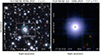 |
Fig. 1. RGB wide filter images of the WFM (left) and NFM (right) MUSE datacube, obtained by collapsing the MUSE datacube in the same spectral regions as the HST/ACS-HCR filters F475W, F625W, and F775W for the WFM data, and F459M, F660N, and F892N for the NFM data. For the NFM data, spectral regions contaminated by instrument features fallen in the filters are excluded. In the WFM image the region studied in this work is highlighted, including PDS 456 and companions, with a dashed white box measuring 80 × 60 kpc2. The cyan box indicates the size (≈23 × 23 kpc2) of the NFM FOV centered on PDS 456. The positions of the nucleus of PDS 456 are indicated with black crosses. |
We use the positions of a handful of point sources identified by Gaia within the WFM MUSE observation field to refine the astrometry of our data. The astrometry of NFM MUSE data is automatically adjusted through alignment with the peak of the continuum emission from PDS 456.
3. WFM observations
3.1. Subtraction of the nuclear and continuum emission
We analyzed the MUSE WFM observations with the purpose investigating the properties of the kpc-scale diffuse gas around PDS 456 by subtracting the BLR emission, the iron transitions, and the continuum emission (hereafter the combination of these emission components is referred to as the nuclear component) from the region associated with the quasar PSF. For the WFM observations this task was complicated by the presence of several continuum sources blended with the quasar. For this reason we did not employ the standard PSF subtraction tools used in literature for the WFM (e.g., CubePSFSub; see below for discussion), and we developed a custom procedure described in detail below.
The initial step consists of extracting the spectrum from a small circular region centered on PDS 456 under the assumption that this area is completely dominated by the nuclear component. In order to derive a spectral model for this emission, we adopted an empirical approach since a purely analytical model results in large residuals, particularly from iron templates. The empirically calibrated model was obtained by performing a spline interpolation of the spectrum using a third-degree polynomial after carefully masking the spectral regions containing narrow emission lines. In order to pinpoint these spectral regions, we relied on a iterative procedure using visual inspection. The model spectral shape is fixed, while we vary the normalization for each spaxel through spectral fitting based on χ2 minimization after masking the spectral regions associated with narrow emission lines. Second-order effects, for example due to wavelength PSF variations, are accounted for with an additional spectral component modeled with a seven-degree polynomial. We note that this additional component had minimal effects on our final result. Finally, the obtained spectral models are subtracted spaxel by spaxel.
To evaluate any potential overestimation or underestimation of the narrow emission lines resulting from the subtraction of the best-fit nuclear component of PDS 456, we examined the [N II]λ6583 Å/[N II]λ6548 Å and [O III]λ5008 Å/[O III]λ4960 Å line ratios. Our analysis indicates that, within the 1σ uncertainties, these ratios match the theoretical predictions (≈1/3; Storey & Zeippen 2000). As a further check we verified that the spatial extension of the nuclear component emission matches the PSF estimated from some point sources in the WFM MUSE field. As a final step, we followed the same procedure described in Sect. 3.2 from Borisova et al. (2016; see also Cantalupo et al. 2019 for further details) in order to eliminate any possible residual emission resulting from the subtraction of the nuclear component and any continuum sources across the entire WFM field of view.
3.2. Morphology and extension of the ionized gas emission
To obtain a 3D map of the ionized gas emission, we used the CubExtractor tool on the datacube after subtracting the nuclear component and the continuum. This tool generates a 3D mask comprising a minimum number of connected voxels (i.e., spatial and spectral elements; MinNVox = 10 000) above a user-defined threshold, and whose line emission is above a minimum signal-to-noise ratio (SN_Threshold = 3). These values are widely used in the literature (e.g., Borisova et al. 2016; Arrigoni Battaia et al. 2019; Cantalupo et al. 2019) to extract extended emission. This method allowed us to trace the circumgalactic medium (CGM) in PDS 456 through the extended emission in the Hβ, Hα, [N II]λ6548 Å, [N II]λ6583 Å [O III] and [S II] optical transitions. We produced the optimally extracted narrowband (NB) images for each detected emission line. These are images obtained by collapsing the only voxels in which the signal-to-noise ratio (S/N) of the emission line is above the SN_Threshold we set.
Figure 2 shows an RGB image produced by including optimally extracted NB images of the extended Hα (red) and [O III] (blue) emission and the white light image (WLI) highlighting the continuum (green) of the original datacube. This image reveals a complex morphology of the CGM around PDS 456, extending to a maximum projected size of ≈46 kpc.
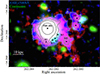 |
Fig. 2. Extended emission surrounding PDS 456, within the region of the WFM-MUSE FoV indicated by a dashed white box in the left panel of Fig. 1. This RGB composite image is generated from the following images: optimally extracted narrowband images of Hα (R) and [O III]λ5008 Å (B) obtained using the CubEx tool, and the white-light image (WLI; G). The black cross symbols indicate the line-emitting companions detected with the Keck Telescope (Yun et al. 2004), ALMA Bischetti19, and in this work with MUSE (see Table 1 for details). MUSE continuum sources are visible in green. The white contours show the surface brightness levels of the [O III] nebula at 10, 50, 100, and 500 10−18 erg s−1 cm−2 arcsec−2. |
3.3. Multiple companions of PDS 456
The CGM emission shown in Fig. 2 also reveals the existence of components resembling bridges that connect various sources marked with black crosses. These sources have the same redshifts as PDS 456, confirmed through the detection of emission and absorption lines with ALMA (B19), and with MUSE data in this study. A comprehensive list of companion sources, including their coordinates, distances from PDS 456, redshifts, and associated tracers, is provided in Table 1.
Companions detected around PDS 456.
Prominent continuum emission is observed from three sources near PDS 456 (i.e., K1, K2, and K3), which were also detected in the K-band continuum using the Near-Infrared Camera on the Keck Telescope (Yun et al. 2004). The MUSE data reveal NaID absorption features, that serve as proxies for neutral gas. The redshifts of these three sources are estimated by fitting the NaID absorption line using the model adopted in Sato et al. (2009) and Perna et al. (2020). The best-fit models are presented in Fig. A.1. The redshifts derived in this way for K1 and K3 match those obtained from CO (3–2) in B19. The absence of these NaID absorption features at the center of PDS456 is consistent with other luminous unobscured AGN (Rupke et al. 2005; Villar Martín et al. 2014; Perna et al. 2017, 2019). Regarding the other continuum sources highlighted in green in Fig. 2, no distinctive features can be discerned to determine their redshifts. A more detailed analysis for this purpose is deferred to future investigations. The MUSE spectra of five sources (M1–M5), show emission lines and a less prominent continuum emission. Notably, the continuum emission for these sources is not visible in Fig. 2, but it is observed in the extracted spectra. Therefore, all eight sources listed in Table 1 exhibit both emission–absorption lines and continuum, identifying them as galaxy companions. Notably, the majority of companions are situated to the west of the central quasar at distances ranging from 9 to 38 kpc.
To determine the nature and properties of most of the PDS 456 companions detected with MUSE, we employed the Baldwin, Phillips, and Terlevich (BPT Baldwin et al. 1981) diagram. As done above, we extracted the same spectra from the datacube nuclear- and continuum-subtracted (Fig. 3, top panel). The emission lines were fit with Gaussian profiles, and the emission line ratios were derived and plotted on the BPT diagram (Fig. 3, bottom panel), with the color bar showing the distance in kiloparsec from PDS 456. The BPT diagram indicates that M1, M4, and M5 fall within the AGN-dominated region, suggesting a significant contribution of AGN illumination. M2 is classified as an HII region, indicating ongoing star formation. Unfortunately, for the companion M3, information on the y-axis was unavailable, and we were unable to assign a specific classification. For the sources M1, M4, and M5, we employed the formula from Keel et al. (2012) to calculate the lower limit of the incident ionizing flux necessary for the observed Hβ line emission, taking into account the distance of these companions from PDS 456. These estimates suggest that the ionizing flux originating from PDS 456 can explain the high ionization observed in the emission lines of all these companions. Therefore, their position on the BPT diagram is not attributed to the presence of an AGN.
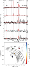 |
Fig. 3. BPT diagram derived from spectral fit results for galaxy companions of PDS 456. The top panel displays the spectra and their best-fit models, while the bottom panel presents the [N II] -BPT diagram, for the galaxy companions of PDS 456. These spectra were extracted from circular regions with a radius of 2 pixels in the datacube, where the nuclear and continuum emission components of PDS 456 have been subtracted. The transparent gray dots show the values from the SDSS survey (credits: Jake Vanderplas & AstroML Developers). The black lines dividing different types of emissions in the BPT diagram are from Kewley et al. (2001). |
3.4. Luminosity and mass of the diffuse ionized gas
In this section our primary objective is to conduct a comprehensive examination of the properties of the large-scale ionized gas surrounding PDS 456. To achieve this we excluded the influence of galaxy companions by utilizing circular apertures with a 5 pixel diameter (i.e., approximately the PSF) centered on their positions.
To estimate the gas properties, we utilized all available optical emission lines within Voronoi regions (see Venturi et al. 2018; Molina et al. 2022). These regions are selected to have a S/N of Hβ higher than 3, and we use the Python tool vorbin for this purpose (Cappellari & Copin 2003). The Hβ is crucial to estimate the extinction of the emission based on the Hα/Hβ line ratio.
The maps of the ionized gas mass estimated from the extended Hα and [O III] emission in Voronoi regions (i.e., MHα and M[O III], respectively) can be seen in Fig. 4. Within each Voronoi region we extracted the spectrum and performed a fit. The fitting procedure involves modeling all emission lines using individual Gaussian profiles with identical widths, except for the [O III] doublet transition. In a few cases, we observed a broader width in [O III] compared to the other emission lines. This discrepancy is attributed to the fact that [O III] is the most reliable tracer for ionized winds and shows a higher S/N, along with Hα, which is more affected by stellar absorption features. The centroid position of each Gaussian was set to have the same redshift, with an adjustment margin equal to the MUSE spectral resolution. The widths obtained from the best-fit models were deconvolved for the MUSE spectral resolution. Adopting these constraints in the modeling helps to minimize the impact of noise, instrumental and sky features, as well as any absorption that might affect the shape of individual emission lines (see also Veilleux et al. 2023).
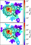 |
Fig. 4. Maps of the extinction-corrected mass estimated from the Hα (top) and [O III] (bottom) emission, divided into Voronoi regions derived to reach a S/N > 3 of the Hβ line emission. The black thick contours in each map represent the S/N levels at 3, 5, 10, 30, and 50 of the [O III] line emission. The black cross gives the position of PDS 456. |
We measured the electron density (ne), color excess (E(B − V)), ionized gas luminosity (Lion), and mass (Mion) derived from the [O III] and Hα emission lines. To estimate ne we utilized the doublet [S II] emission line ratio, as described in Osterbrock & Ferland (2006). The errors in ne were determined by applying a bootstrap algorithm for a sample of ne values obtained by randomly varying the intensities of the [S II] emission lines within 1σ error. In cases in which the S/N of the [S II] doublet lines was less than 2.5, which tends to occur at larger distances from the quasar, we adopted a fixed value of ne = 150 cm−3, which represents the minimum value calculated through the [S II] line ratio in the outer regions. In this way, we found that ne is ≈600 cm−3 at the center, decreasing to ≈150 cm−3 in the outer regions. To correct for dust extinction in the observed flux, we estimated E(B − V) using the Balmer decrement Hα/Hβ flux ratio. We applied the Calzetti et al. (2000) attenuation law, assuming an intrinsic Balmer ratio Hα/Hβ of 2.86 for gas at an electron temperature of Te = 104 K (Osterbrock & Ferland 2006), and utilizing RV = 3.12. Near PDS 456, we obtained E(B − V) ranging from 0.2 to 1.1 mag, decreasing at larger distances. Then, we estimated the total luminosity, corrected for dust extinction, in Hα and [O III] to be  and
and ![Mathematical equation: $ \log(L_{[{\mathrm{O}\,\textsc{III}}]}/\mathrm{erg~s}^{-1}) = 43.43_{-0.30} ^{+0.26} $](/articles/aa/full_html/2024/06/aa49201-24/aa49201-24-eq2.gif) .
.
To estimate Mion, we used both the Hα and [O III] transition luminosity, corrected for dust extinction, according to the Osterbrock & Ferland (2006) formula
![Mathematical equation: $$ \begin{aligned} M_{[{\text{O}}{\small {{\text{ III}}}}]} = 8 \times 10^7\,{M_{\odot }} \biggl ( \frac{C}{10^{[\mathrm{O/H}]-[\mathrm{O/H}]_{\odot }}} \Biggr ) \biggl ( \frac{L_{\rm [OIII]}}{10^{44}~\mathrm{erg~s}^{-1}} \Biggr ) \biggl ( \frac{n_{\rm e}}{500~\mathrm{cm}^{-3}} \Biggr )^{-1} \end{aligned} $$](/articles/aa/full_html/2024/06/aa49201-24/aa49201-24-eq3.gif) (1)
(1)
(or Carniani et al. 2015; Bischetti et al. 2017), where C is the clumpiness of the gas (i.e.,  ), [O/H] is the oxygen abundance relative to hydrogen, and the formula
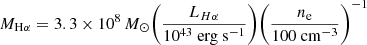 (2)
(2)
by Nesvadba et al. (2017) and Leung et al. (2019). In both cases, we assumed a Te = 104 K and solar metallicities. We corrected M[O III] by multiplying it by a factor of three, as determined by F17 due to the discrepancies between mass estimates obtained using Eqs. (1) and (2). The total mass, as derived through the Hα and [O III] emission lines, is  and
and  , respectively. These are two to three orders of magnitude lower than the virial dynamical mass of ∼1010 M⊙ derived within 1.3 kpc by B19.
In Fig. 5 the total L[O III] measured for PDS 456 is compared to those derived for other samples of Type 1 quasars over a large redshift range (z ∼ 0.1 − 4). PDS 456 clearly lies at the brightest end of the L[O III] distribution for sources at z ≲ 1. Moreover, its L[O III] is also consistent with that observed for the bulk of the quasar population at Cosmic Noon (e.g., Coatman et al. 2019) supporting the role of PDS 456 as a local counterpart of high-z quasars; it is smaller by a factor of tens only when compared to that of hyper-luminous quasars like those in the WISE/SDSS selected hyper-luminous (WISSH) survey.
 |
Fig. 5. Total observed [O III] luminosity (L[O III]) of PDS 456 (red star) compared with that measured for other samples of Type 1 quasars in the redshift range z ∼ 0.1 to ∼4. The quasars at z < 1 are from Husemann et al. (2013; green dots), Husemann et al. (2014; yellow dots), Liu et al. (2014; purple dots), and Perna et al. (2017; orange dots). Quasars at z > 1 are from Coatman et al. (2019; blue dots) and Bischetti et al. (2017; red dots). |
3.5. The large-scale [O III] ionized outflow
In this section we reveal the presence of an ionized outflow based on the kinematics of the gas. To achieve an adequate S/N in the spectra, we binned the final nuclear- and continuum-subtracted datacube into 3 × 3 pixel regions1, equivalent to 1.87 × 1.87 kpc2. Each spectrum extracted from this binned datacube was analyzed to model only the [O III] line emission, which was used as the best proxy for the outflow. We adopted a single- or double-Gaussian model according with the Bayesian information criterion2 (BIC; Schwarz 1978). From the best-fit models we derived the velocity maps, v50, v90, and v10, representing the velocities containing a specific percentage of the total integrated flux of the emission line. Additionally, we calculated w80, defined as v90 − v10 (see Harrison et al. 2014). Commonly, the latter is used to trace kinematic properties associated with outflows (Vega Beltrán et al. 2001; Collet et al. 2016; Harrison et al. 2016).
In Fig. 6 the w80 map reveals velocities exceeding 500 km s−1 in the vicinity of the PDS 456 core. These values gradually decrease to ≈300 km s−1 at larger radii and decrease further near the location of the companions. The v50 map reveals negative velocities with v50 < −100 km s−1 to the east of the quasar’s position (Fig. 6). On the west side the velocities are in the range |v50| < 50 km s−1, which is consistent with the maximum velocities observed in the CO (3–2) disk probed in ALMA data (B19). Velocities for the blue and red wings are determined using v10 and v90, respectively. These measurements indicate an east–west velocity gradient, with the blue wings extending to −450 km s−1 in the east and the red wings reaching 250 km s−1 in the west.
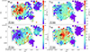 |
Fig. 6. Maps of w80 (top left), v50 (top right), v10 (bottom left), and v90 (bottom right) of the [O III] emission line. These maps provide an overview of the widths and velocity shifts from the entire [O III] profile. In each panel, the black thin contours represent the S/N levels shown in Fig. 4. The black thick contours in the center of the figure depict the molecular outflow, detected in B19. These contours correspond to the emission levels of 1, 4, 8, and 10 mJy. The white cross gives the position of the quasar. The white lines in each map represent 2σ Gaussian-smoothed contours that enclose the regions where w80 exceeds 400 km s−1. |
The kinematic maps highlight the following features: a notable velocity gradient in the east–west direction with negative to positive v50 values, and perpendicular to the gradient of the compact molecular disk; a central w80 exceeding ≈ 500 km s−1, more than twice the central velocity dispersion of the molecular gas (i.e., σvel = w80/1.09/2.355 for a Gaussian profile); and v10 < −300 km s−1, aligning with the extended CO (3–2) outflow represented by thick black contours in Fig. 6, which is also blueshifted. These findings collectively suggest the presence of outflowing gas, which is further supported by the analysis of the NFM data presented in Sect. 4.2. The latter reveal an unmistakable blueshifted outflow detected in Hα within ≈3 kpc of the center, aligned with the direction of the CO (3–2) outflow.
This information can be used to point out the region where the outflow dominates in the WFM MUSE data, essential for establishing the maximum projected distance of the [O III] outflow. As a rough estimate, we calculate an average σvel of the Hα outflow in NFM MUSE data of ∼150 km s−1 (see Fig. 9). This corresponds to a w80 = 400 km s−1 and can be used as a reliable tracer for the [O III] outflow. Applying this criteria, we observe that the region where the ionized outflow dominates has a maximum projected size of ≈20 kpc, as shown by the white contours in each map in Fig. 6.
In conclusion, our findings reveal compelling evidence of an outflow with a potential maximum projected distance of 20 kpc. This ionized outflow is characterized by w80 ≥ 500 km s−1 in the center, and also exhibits blueshifted and redshifted velocities up to −450 km s−1 and 250 km s−1 to the east and west of the quasar, respectively.
3.6. No rotational pattern in the ionized disk
The ALMA data on PDS 456 reveal a compact (effective radius of 1.3 kpc) and nearly face-on (i ∼ 25 deg) molecular disk in CO (3–2) with a peak-to-peak velocity of 100 km s−1 along the N–S direction (see Fig. 4 in B19). Under the assumption that the molecular and ionized phases of the gas disk share the same velocity gradient (Levy et al. 2018), the kinematics of the ionized gas, probed with both [O III] and Hα, do not reveal an ionized counterpart to this disk. Instead, there is a gradient in velocities along the E–W direction (see the v50 map in Fig. 6), perpendicular to the velocity gradient of the molecular disk and indicative of the outflow kinematics. Therefore, we suggest that the ionized disk is not detected, likely due to the rotational velocity of the disk being comparable to the MUSE spectral resolution, and the kinematics being dominated by the outflow.
4. NFM observations
The AO-NFM MUSE data provide us with an unprecedented zoom-in of the central ∼24 × 24 kpc2 region of PDS 456 with high spatial resolution (∼280 pc), reaching a surface brightness limit of ≈3 × 10⁻¹⁹ erg s−1 cm−2 arcsec−2 (3σ). This allowed us to study in detail the morphology and kinematics of the ionized gas on the same scales of the molecular outflow Bischetti19.
4.1. PSF and continuum subtraction
We used CubExtractor tools to subtract the PSF contribution of the quasar (including emission non-resolved from host-galaxy or NLR), and the continuum of the sources in the datacube. In particular, the CubePSFSub tool uses an empirical approach for the PSF subtraction at each wavelength based on pseudo-broadband images produced from the cube itself as described in detail in Cantalupo et al. (2019). This tool is specifically designed to extract faint and extended line emission on large scales from the bright continuum PSF of an isolated quasar assuming that it is the dominant source of continuum emission in the PSF area as it is in our NFM observations (e.g. Borisova et al. 2016; Arrigoni Battaia et al. 2019; Farina et al. 2019; Cantalupo et al. 2019; Travascio et al. 2020).
As we mention in Sect. 2, the [O III] and Hβ transitions are not covered because they fall in the NaID notch filter from the laser guide star, that contaminate that spectral region. Hence, we perform the PSF and continuum subtraction on a datacube in which we mask the spectral regions including Hα, [N II] doublet, and [S II] doublet emission lines. The analysis to extract with CubExtractor the extended emission in AO-NFM MUSE data is the same used for the WFM MUSE data described in Sect. 3.2. We extracted the extended emission (in the Hα, [N II], and [S II] transitions) by setting, in the CubEx function, a S/N threshold of 3 and a minimum number of connected voxels of 3000.
4.2. High-resolution view of the ionized versus molecular spatially resolved outflows
The morphology of the Hα emission shown in Fig. 7 (obtained from the AO-NFM observations) extends in a northeast direction with respect to the quasar, along the same direction as both the large-scale ionized and extended molecular outflows. The emission structure shows two emission peaks connected by a diffuse extended component. One peak is located close to the nucleus, while the other is situated 2 kpc east of the first, exhibiting a thick shell-like geometry. The morphology of this structure closely overlaps that of the molecular outflow (B19; gray contours), suggesting a multi-phase composition of the outflowing gas. Due to the lower sensitivity of AO-NFM MUSE data compared to that in the WFM MUSE data presented in the previous sections, we do not detect a similar elongated structure in the south direction.
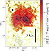 |
Fig. 7. MUSE NFM surface brightness map of the Hα emission. The black contours show the S/N levels of the Hα emission of 3, 5, and 10. The gray contours show the morphology of the blueshifted CO (3–2) molecular outflow (B19), at the emission levels of 1, 4, 8, and 10 mJy. The black circles indicate regions affected by significant residuals in the PSF subtraction due to the quasar and a nearby continuum source. |
Figure 8 shows the maps of the first (top panel; vshift) and second (bottom panel; σvel) moment of the Hα flux distribution obtained with the Cube2Im tool (see Borisova et al. 2016). The thick gray contours overlaid on the maps represent the morphology of the molecular outflow detected by B19. In the ≈1.4 kpc thick shell-like region traced by the Hα emission, the vshift values are lower than −150 km s−1 and the σvel values are higher than 120 km s−1. These velocities differ from those present in the remaining regions, showing vshift between −50 and 50 km s−1 and σvel around < 100 km s−1. The spatial correlation between this shell and the molecular and large-scale ionized outflows suggests that this perturbed emission, up to σvel of 200 km s−1, is likely tracing an outflowing gas front.
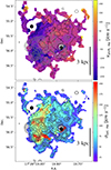 |
Fig. 8. First (top) and second (bottom) moment of the flux distribution of the Hα emission obtained with the Cube2Im function in CubExtractor, representing the vshift and σvel maps. The gray contours show the morphology of the extended (up to ≈5 kpc) blueshifted CO (3–2) molecular outflow, detected by B19, at the emission levels of 1, 4, 8, and 10 mJy. The black circles and contours are the same as in Fig. 7. |
Figure 9 displays the spectrum of the Hα transition, zoomed in on the black Hα transition, extracted from the thick shell-like region with σvel higher than 90 km s−1 (maximum σvel in the center of the compact molecular disk). The spectrum of the Hα line emission (in red) from the WFM MUSE data, extracted from the same region, and the spectrum of the CO (3–2) outflow (in green) from B19, are overlaid. The Hα-NFM and the CO (3–2) spectrum are normalized at the peak of the emission line, while the Hα-WFM spectrum is normalized to match its blueshifted wing with the Hα-NFM. These spectra are plotted as a function of vshift with respect to the wavelength of the relative transition at the systemic redshift of the quasar. By comparing the maximum velocities reached by the wings of the emission lines, we observe identical vshift values for the Hα line emission in the NFM and WFM MUSE data. We conclude that the molecular and ionized outflows have similar kinematics. These similarities (i.e., extent, morphology, kinematics) strongly suggest the co-existence of different gas phases within these outflows. Moreover, the morphology of the emission of the CO (3–2) molecular and the Hα ionized outflows may depend on the spatial variation of density, implying a clumpy structure of the gas (Baron & Netzer 2019), although it could also be related to spatially varying emissivity or intrinsic dust absorption.
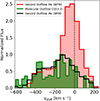 |
Fig. 9. Spectra extracted from nuclear- and continuum-subtracted MUSE WFM (red; Hα) and NFM (black; Hα) datacubes, and from the ALMA data (green; CO (3–2)), in the region where the Hα outflow is observed in NFM MUSE data. |
4.3. Ionization mechanisms of the outflowing gas
In this section we discuss the ionization mechanism of the outflowing gas in Hα. We used the spatially resolved [N II]/Hα and [O III]/Hβ line ratios measured in NFM and WFM MUSE data, respectively, as key components in the diagnostic BPT diagram.
Figure 10 (top panel) shows a smoothed map of the [N II]/Hα emission line ratio obtained from the respective optimally extracted images derived with Cube2Im. Most of the emission associated with the outflow region exhibits a drop in the log([N II]/Hα) (< − 0.3) with respect to the values in the entire map. Unfortunately, no other relevant emission lines fall in the spectral range covered by NFM MUSE data, while the WFM MUSE data cannot provide line ratio estimates at the same spatial resolution of NFM data. The low [N II]/Hα line ratio weakens the hypothesis of shock excitation, which is typically associated with an increase in the [N II]/Hα and [S II]/Hα line ratios in the regions with highest values of σvel (e.g., Leung et al. 2019). This could be an indicator of star formation occurring in the outflowing gas (e.g., Maiolino et al. 2017) or AGN ionization followed by the recombination of hydrogen atoms in a photon-dominated scenario, depending on the [O III]/Hβ line ratio (e.g., O’Dell et al. 2009). To distinguish between these scenarios, the bottom panel in Fig. 10 presents a map of the [O III]/Hβ line ratio, derived from the optimally extracted NB images obtained from WFM MUSE data with the CubExtractor tools by setting a S/N threshold of 3. We observe that the [O III]/Hβ line ratio tends to increase in the region of the outflow detected in Hα emission in the NFM MUSE data.
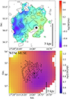 |
Fig. 10. Emission-line ratio maps for the extended gas around PDS 456. Top panel: [N II]/Hα emission line ratio map, at S/NHα > 2.5, whose pixel size is five times larger than the native pixel in NFM MUSE data, which corresponds to ∼1.3 FWHMPSF. The black dot gives the position of the central quasar, and has the FWHM size of the PSFNFM. Bottom panel: Map of the [O III]/Hβ line ratio estimated through the [O III] and Hβ optimally extracted NB images extracted from the WFM MUSE data with CubExtractor. The black contours represent the S/N levels of the Hα emission extracted from the NFM MUSE data at 3, 5, and 10. |
This, combined with the [N II]/Hα line ratio, agrees with the results of Hinkle et al. (2019), who suggest that outflowing gas showing a higher [O III] /Hβ line ratio and a lower low-ionization line ratio (i.e., [N II] / Hα, [S II] / Hα, [O I] / Hα) than those of the host galaxy ISM implies a difference in the ionization parameter. In addition, Mingozzi et al. (2019) explain that outflowing gas in the NLR of Seyfert galaxies shows a low [N II]/Hα line ratio as it is directly illuminated by the AGN continuum. This may result from the Hα emission tracing matter-bound clouds within the outflow, which dominate the emission in the ionization cone (see Mingozzi et al. 2019, for a discussion).
5. Energetics of the ionized outflow in PDS 456
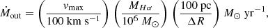
In this section we estimate the properties (Mout, Ṁout, Ėkin, and Ṗout) of the ionized outflows in PDS 456 probed with Hα emission in NFM MUSE data (up to ≈3 kpc scales) and [O III] emission in the WFM MUSE data (up to ≈12 kpc scales). First, we compare the properties of the extended ionized outflow probed with WFM MUSE data with those found in other AGN. Most of them are reported in F17 and updated in B19, while others values can be found in Fluetsch et al. (2019) and Speranza et al. (2024). F17 assembled a sample of cold molecular outflows (CO, OH) and warm ionized outflows ([O III], Hα, Hβ) from AGN spanning a broad range of redshifts (z < 3) and bolometric luminosities. Most of these AGN were studied using integral field unit (IFU) data. Subsequently, given that the morphology and kinematics of the 1–3 kpc scale (excluding blob B, as detected by B19, located 5 kpc south of PDS 456; see Fig. 7) blueshifted CO (3–2) and Hα outflows observed in the MUSE-NFM data suggest that these components are part of the same multi-phase outflow and are likely driven by the same past AGN feedback event (Sect. 4.2), we proceed to compare the properties and energy of these two outflow phases. This is crucial in order to explore the distribution of energy in different outflow phases and its correlation with distinct mechanisms that determine energy efficiency coupling. We therefore calculate the integrated properties of the ionized outflow. To achieve this, we extract a spectrum from the WFM and NFM MUSE data in regions dominated by the outflow, defined as the region where w80 ≥ 400 km s−1 (see Sect. 3.5) and the region where σvel is larger than 90 km s−1 (see Sect. 4.2), respectively. In both cases we define the outflow based on a fitting model with two Gaussians: a narrow one (σvel ≈ 76 km s−1) representing the systemic non-outflowing gas, and a broader one (σvel ≈ 240 km s−1) tracing the outflow component (see Fig. 11). From the best-fit model of the outflowing component, we derive some parameters for estimating additional outflow properties, and their associated 1σ uncertainties are calculated using a bootstrap algorithm with 104 iterations. This process involves propagating the errors obtained from the best-fit models of the initial spectra.
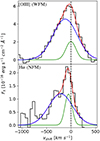 |
Fig. 11. Spectra, in velocity units, extracted from the regions where the outflow dominates the emission (see text for details), in WFM (top panel) and NFM (bottom panel) MUSE data. Shown are a zoomed-in images of the [O III] (top panel) and Hα (bottom panel) transitions. The red lines show the best-fit model consisting of the combination of two Gaussian components: a narrow one (green) and a broader one (blue), tracing the outflow. |
We derive the maximum velocity (i.e., vmax≡ vshift +2× σvel; F17) and the observed integrated fluxes, which is corrected for dust extinction. The dust extinction, characterized by E(B − V)≈0.52 mag, is estimated from the Hα/Hβ line ratio observed in the central 5 × 5 kpc2 region in the WFM MUSE data, with the same method used in Sect. 3.4. This value is consistent with the results obtained by Reeves et al. (2021) for PDS 456 and is also used for the extinction correction of the Hα outflow.
The energetic properties that we derive for the outflow are dependent on ne. Most of the studies of spatially resolved kiloparsec-scale outflows in AGN assume a uniform ne value, for example < 500 cm−3 (Kakkad et al. 2016, Rupke et al. 2017, F17, Carniani et al. 2015, Bischetti et al. 2017) or > 1000 cm−3 (Müller-Sánchez et al. 2011; Santoro et al. 2018; Förster Schreiber et al. 2019; Baron & Netzer 2019). On the other hand, several studies show that ne of the outflows in AGN can vary between ∼50 cm−3 and 106 cm−3 (Perna et al. 2017; Kakkad et al. 2018; Rose et al. 2018; Baron & Netzer 2019; Holden et al. 2023; Venturi et al. 2023). In addition, uncertainties on ne can also be large due to the limited data quality and the strong assumptions adopted in each method (Baron & Netzer 2019; Davies et al. 2020; Revalski et al. 2022).
For a proper comparison of the [O III] outflow properties in PDS 456, as observed in WFM MUSE data, with those reported in F17, we use the same electron density value, ne = 200 cm−3, as employed in their study. The mass of the [O III] outflow is derived using the Eq. (1) and, based on F17, the outflow mass estimated with the [O III] line is systematically lower by a factor of 3 than that derived with Hα or Hβ transitions, which are robust estimators of the mass. Therefore, we multiply the M[O III] in Eq. (1) by a factor of 3. To calculate the mass outflow rate of the [O III] outflow we use the formula in F17 assuming a cone geometry:
![Mathematical equation: $$ \begin{aligned} \dot{M}_{\rm out} = 3 \times \Biggl ( \frac{M_{[\mathrm{OIII}]} \times { v}_{\mathrm{max}}}{R_{\mathrm{out}}} \Biggr ) . \end{aligned} $$](/articles/aa/full_html/2024/06/aa49201-24/aa49201-24-eq8.gif) (3)
(3)
Here Rout is the maximum radius up to which high-velocity gas (i.e., w80 > 400 km s−1) is detected, following the approach used in the F17 sample. Specifically, to take into account the uncertainties in the estimates of the radius of the bulk of the outflow, we compute the 50th percentile (the median value), as well as the 16th and 84th percentiles of the distances, weighted by the fluxes. The main properties of the total outflow traced from the [O III] emission in WFM MUSE data are listed in Table 2 (top row).
Properties of the ionized (Hα, [O III]; top subtable) and molecular (CO (3–2); bottom subtable in B19) outflows in PDS 456.
For the [O III] outflow detected in the WFM MUSE data, we estimate Mout = (2.3 ± 0.2)×107 M⊙, 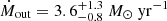 , and Ėkin = (4.2 ± 1) × 1041 erg s−1. In Fig. 12 we report the plots Lbol versus vmax (top panel), Ṁout (central panel), and Ėkin (bottom panel). The ionized outflow in PDS 456 exhibits a vmax that is consistent with the scatter of the relation in F17, at fixed Lbol. The vmax of the total molecular outflow in PDS 456 Bischetti19 reaches a value of around 1000 km s−1, which is consistent with the values observed in the ionized outflow. Furthermore, it falls within the lower limit of the scatter observed in the population of molecular outflows. The values of Ṁout and Ėkin of the ionized outflow in PDS 456 are ≈2–4 orders of magnitude lower than those estimated in the sample of F17 at a similar Lbol. The properties of the molecular outflow in PDS 456 are slightly below (at the lower end) the extrapolation of the high-Lbol points for the molecular outflow in F17. Ṁout and Ėkin of the total ionized outflow observed in PDS 456 are consistent with those of the well-studied outflow in the quasar XID2028 at z ∼ 1.59 by using high-resolution JWST data (Cresci et al. 2023; Veilleux et al. 2023). The ionized outflow in XID2028 exhibits higher velocities (≈1100 km s−1) compared to that in PDS 456, but shows comparable extent (≈10 kpc), Mout (107 − 108 M⊙), and Ṁout (3 − 6 M⊙ yr−1). However, the morphology of the ionized outflow and radio lobes in XID2028 suggest that they are connected, possibly indicating a jet-driven outflow. On the contrary, the orientation and size of the ionized outflow and radio jet (up to 200 pc in size) in PDS 456 are uncorrelated, suggesting a radiative-driven outflow mechanism. On the other hand, if we consider the [S II] line ratio to estimate ne of the [O III] outflow (Osterbrock & Ferland 2006), we obtain a value of approximately 400 cm−3. Assuming this to be the most accurate value, both Ṁout and Ėkin must be rescaled by a factor of two compared to those reported in Fig. 12 (see Table 2).
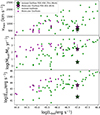 |
Fig. 12. vmax (top panel), Ṁout (central panel), and Ėkin (bottom panel) of the molecular and ionized outflow in PDS 456 (star symbols) vs. Lbol. We compare these values with those of ionized and molecular outflows reported in F17, B19, Fluetsch et al. (2019), and Speranza et al. (2024). For the estimation of the ionized outflow properties, an ne of 200 cm−3 from F17 was used. |
Thanks to the superb resolution of the NFM MUSE data we are able to directly compare the ionized outflow traced by the Hα, and the CO (3–2) molecular outflows discovered by B19, within ≈1–3 kpc from PDS 456 (see Fig. 7). For the Hα outflow, we derive ne = (500 ± 200) cm−3 using the [S II] line ratios (Osterbrock & Ferland 2006; Jiang et al. 2019), which is consistent with ne derived for the [O III] outflow observed in WFM MUSE data. The mass of this Hα outflow is estimated using Eq. (2). To estimate the mass outflow rate, we adopt the formula from Husemann et al. (2019),
 (4)
(4)
which provides the mass rate within an outflowing shell of thickness ΔR. The key properties of the Hα ionized outflow in the NFM MUSE data are summarized in Table 2 (bottom row). The values of Mout, Ṁout, and Ṗout for the Hα ionized outflow detected in NFM MUSE data are about one order of magnitude lower than those for the molecular outflow. The distinct gap between the properties carried by the ionized and molecular outflows is also evident for the total outflows, as discussed in the previous section. These discrepancies suggest that the ionized component of the outflow makes a negligible contribution in terms of energy. This finding is inconsistent with the expected energy equivalence based on the high-Lbol relation presented in F17.
Menci et al. (2019) noted that the mass outflow rate depends strongly on the direction of the outflow with respect to the plane of the disk. In particular, the mass rate of outflows is highest in the direction of the disk and decreases as the outflow moves away from the disk. This is due to the fact that the density of the gas in the disk is higher than that in the outflowing gas, and the mass outflow rate is proportional to the density of the gas. Based on this scenario, the observed difference in mass outflow rates between ionized and molecular outflows at the ≈1–3 kpc scales, as well as the overall outflow, may be attributed to the different directions of these outflows in relation to the disk’s plane. In this scenario the molecular outflow could be triggered by nuclear winds impacting the ISM gas, while the ionized outflow might result from the radiative pressure of AGN photons on NLR clouds. However, this hypothesis needs to be confirmed through further detailed analysis of the multi-phase outflow observed at the ≈1–3 kpc scales.
6. Scenarios for the expansion of multi-phase galactic-scale outflows
We discuss here a variety of possible scenarios that could explain the properties of the multi-phase outflow in PDS 456. B19 suggest that in a high-Lbol regime the ionized outflow may represent a significant fraction of the outflow mass, reducing the discrepancy between the low momentum boost measured from the molecular phase alone with the expectations for an energy conserving expansion of the nuclear UFO. Nonetheless, the momentum boost of the multiphase, galaxy-scale outflow of (Ṗmol + Ṗion)/Ṗrad ≈ 0.37 is not consistent with an energy-conserving (i.e., non-radiative) expansion powered by the quasar, which predicts values in the range 5–10 (Zubovas & King 2012).
6.1. Intermittent AGN phases scenario
One possibility to reconcile the observations with an energy conserving expansion relies on the fact that the outflow might have been inflated during a previous AGN phase. Considering a velocity ≈300 km s−1, it takes the outflow ∼1 Myr to expand to the 0.3 kpc scale of the compact outflow, and ∼10 Myr to reach the 3 kpc size of the extended outflow. Even 1 Myr is longer than the expected typical duration of a single AGN episode, which is estimated by both statistical (Schawinski et al. 2015) and analytical arguments (King & Nixon 2015) to be < 0.1 Myr. It thus appears likely that the outflows that are observed now were inflated by multiple previous AGN episodes. This scenario would also reconcile the kinetic power of the galactic-scale outflow in PDS (Fig. 12) with that expected from the F17 relations, which reflect the overall quasar population, and thus the long-term average of Lbol. The luminosity during a single AGN episode is not constant; rather, it probably decreases as the accretion disk is consumed, while feedback prevents more material from reaching the disk efficiently (King & Pringle 2007). Zubovas & Nardini (2020) showed that in such cases, outflow properties tend to correlate better with the long-term average AGN luminosity than the instantaneous value. Given that the current luminosity of PDS 456 is Lbol ≃ 0.7 LEdd (Reeves et al. 2000; Nardini et al. 2015) it is very likely that the long-term average luminosity is much lower. The UFO revealed in X-rays, on the other hand, probably evolves on sub-year timescales and so closely tracks the present-day luminosity. Assuming that the nuclear wind always had kinetic power equal to ∼20% Lbol, as today, a long-term average luminosity 10–20 times lower than the present-day value would bring the outflow properties in line with the expectation of an energy-driven scenario. Such a low average luminosity is easy to achieve: it requires the product of AGN duty cycle over the past 1–10 Myr and the average Eddington factor during an episode to be of order 0.035–0.07. The AGN duty cycle is defined in Zubovas & Nardini (2020) as δAGN = tep/tr, where tep represents the duration of the AGN episode, which is a measure of how long the AGN remains in an active state, while tr refers to the recurrence timescale, which determines the frequency of AGN activity. By definition, the average luminosity during an episode is below Eddington (i.e., LAGN > 0.01 × LEdd), so the duty cycle has to be somewhat higher than the population average of ∼0.07 to achieve this. Moreover, Zubovas et al. (2022) suggested that AGN episodes may be clustered hierarchically in time, with longer phases lasting 107 yr (as suggested by Hopkins et al. 2005) during which multiple AGN events occur, each lasting ∼105 yr.
6.2. Radiation-pressure driven outflow scenario
Yet another possibility, as suggested by B19, is that radiation pressure on dust has triggered these outflows in PDS 456, implying a value of the momentum load of galactic-scale outflow around unity (Ishibashi & Fabian 2014; Costa et al. 2018). This scenario might be supported by the detection of outflowing emission traced by blueshifted high-ionization emission lines in the mid-IR (i.e., 15.56 μm [Ne III] and 14.32 μm [Ne V]) with a velocity higher than found for [O III] and Hα, and therefore related to an inner highly extincted ionized wind component (e.g., Spoon & Holt 2009), or the detection of dust emission co-spatial with the multi-phase outflow.
6.3. Star-formation and radio-jet driven scenario
An origin of the multi-phase outflow in PDS 456 due to star formation activity or one linked to the power of a radio jet both seem to be unlikely. Specifically, B19 excluded a dominant starburst contribution to the outflow acceleration since the kinetic power of the molecular outflow is significantly greater than that expected for a wind triggered by a star formation activity with a SFR ≃ 50 − 80 M⊙ as observed in PDS 456.
Yang et al. (2021) detected a complex radio structure comprising a radio core, a radio jet, and a diffuse component. These radio components extend to distances of ∼370 pc from the quasar, with luminosities of log(Lνν/erg s−1) = 40 (ν = 1.66 GHz), and log(Lνν/erg s−1) = 39.3 for the radio core and jet, respectively. A strong correlation between the galactic-scale outflows and the radio jets seems unlikely because the radio luminosity is more than two orders of magnitude lower than the kinetic power associated with the galactic-scale outflows, although based only on the luminosity at ν = 1.66 GHz. Moreover, the scales and orientation of the radio emission (see Fig. 2 in Yang et al. 2021) are uncorrelated with those of the ionized and molecular outflows (Figs. 6 and 8), suggesting that they are not related.
7. Summary and conclusions
We carried out the analysis of the first VLT/MUSE WFM and AO-NFM observation of the nearby (z = 0.185) luminous (Lbol ∼ 1047 erg s−1) quasar PDS 456. These data provided us with the opportunity of mapping with unprecedented detail the ionized emission from a luminous quasar with a multi-scale multi-phase outflow.
Specifically, with the WFM MUSE data, we were able to investigate the environment and a kiloparsec-scale outflow. The AO-NFM MUSE data offered an unmatched spatial resolution of ∼280 pc, enabling us to accurately study in detail the morphology and kinematics of the ionized outflow and compare it with those of the molecular outflow, with equal resolution and at the same scales. Our analysis provided the following key results:
-
PDS 456 resides in a complex environment characterized by the diffuse emission of ionized gas extending up to a maximum projected distance of ∼46 kpc, which traces the CGM and the presence of multiple line-emitting companion galaxies within ∼30–40 kpc (see Fig. 2). We estimate the mass of the emitting ionized gas, through the [O III] and Hα emission lines, ∼3 and ∼9×10⁷ M⊙, respectively (see Sect. 3.4). These findings match the theoretical and observational expectations suggesting that hyper-luminous quasars live in overdense regions in terms of companion galaxies (Wagg et al. 2012; Decarli et al. 2017; Trakhtenbrot et al. 2017; Bischetti et al. 2021; Nguyen et al. 2020; Perna et al. 2023) and reservoir of gas (Bowen et al. 2006; Prochaska & Hennawi 2009; Farina et al. 2013).
-
We also discover the existence of an ionized outflow (vmax ∼ 600 km s−1), mainly detected in [O III], and characterized by a maximum projected size of ≈20 kpc and a velocity gradient along the east–west direction (see Sect. 4.2; Fig. 6).
-
Ṁout and Ėkin of the [O III] ionized outflow in PDS 456 are 2–4 orders of magnitude less than those derived in objects with similar Lbol in literature (Fiore17; Bischetti19; Fluetsch et al. 2019; Speranza et al. 2024), while the measured value of vmax ≈ 600 km s−1 is consistent with those typically found in other quasars (see Fig. 12).
-
The total multiphase outflow expands in a regime not consistent with energy conservation, contrary to what might be expected given its scale (King & Pounds 2015). In Sect. 6.1, we discuss in detail the intermitted AGN phase scenario, that could provide an explanation for this finding.
-
The spatially resolved Hα emission in the AO-NFM MUSE data partially traces the same [O III] outflow detected with WFM MUSE data down to ≈1 − 3 kpc scales from the quasar. The high resolution enables us to reveal a thick shell-like geometry (see Fig. 7).
-
The remarkable similarity in morphology, direction, and kinematics between the Hα outflow detected in the NFM MUSE data and the extended CO (3–2) molecular outflow strongly suggests that these two components belong to the same multi-phase outflow and could be driven from the same past AGN feedback episode (see Figs. 8 and 9).
-
The molecular phase dominates the kinetic power of the multi-phase galaxy-scale outflow, with Ṁmol and Ṗout that are about 1 order of magnitude larger than the values for the ionized outflow.
In conclusion, our analysis of the MUSE data reveals novel and important details on the complex interplay between the different phases of AGN-driven outflows extending up to ∼20 kpc (i.e., interacting with the CGM), and the richness of circumgalactic environment of PDS 456. This may help in planning and performing future multi-band investigations of the properties of the luminous quasars shining at cosmic noon.
We highlight that deeper MUSE observations in both WFM and NFM modes would allow us to enhance and broaden our analyses. Specifically, these WFM observations could reveal a more extensive CGM structure associated with PDS 456 across all optical transitions. Data with a higher S/N may help in identifying a fainter wing of the [O III], suggesting the presence of a less dominant or more obscured outflow at higher velocities. In addition, deeper MUSE NFM observations would be crucial for investigating the presence of more extended quiescent and outflowing ionized gas. This is very important for comparing the differences in clumpiness between the ionized and molecular phases of the gas and improving our ability to produce spatially resolved ne maps of the outflow, thanks to the high S/N maps of [S II] emission lines.
Furthermore, JWST/NIRSpec-IFU data (filter G235H/F170LP) and MIRI-IFU data (filter F770W) have recently been acquired. These data are crucial to investigate both hot molecular and highly extincted ionized gas, potentially revealing additional phases of the outflow in PDS 456 (Spoon & Holt 2009; Bianchin et al. 2022). Additionally, the rest-frame near-IR H2 emission line can be used as a valuable tracer for shocks and can contribute to a clearer understanding of the main expansion mechanism in the shell.
The analysis employing the Voronoi regions discussed in Sect. 3.4 is not applicable in this context due to contamination in defining a region with specific kinematics. Instead, the Voronoi analysis is valuable for exploring the global properties of the gas, necessitating information from multiple lines.
The BIC statistic is calculated as the difference between χ2 + kln(N), where N represents the number of data points and k is the number of free parameters in the model, for the single- and double-Gaussian models. Following this approach, a single-Gaussian profile is considered the best-fit model when the difference (BICsingle − BICdouble) is less than 10, as done in Vietri et al. (2020).
Acknowledgments
We thank the referee for the careful reading of the manuscript and the helpful comments. Based on observations made with ESO Telescopes at the La Silla Paranal Observatory as part of the ESO programme ID 0103.B-0767(A-B). This project was supported by the European Research Council (ERC) Consolidator Grant 864361 (CosmicWeb) and by HORIZON2020: AHEAD2020-Grant Agreement n. 871158. Support from the Bando Ricerca Fondamentale INAF 2022 Large Grant “Toward an holistic view of the Titans: multi-band observations of z > 6 quasars powered by greedy supermassive black-holes” is acknwoledged. EP and GV acknowledge the PRIN MIUR project ‘Black hole winds and the baryon life cycle of galaxies: the stone guest at the galaxy evolution supper’, contract number 2017PH3WAT). EP and FT acknowledge funding from the European Union – Next Generation EU, PRIN/MUR 2022 2022K9N5B4. GC acknowledges the support of the INAF Large Grant 2022 “The metal circle: a new sharp view of the baryon cycle up to Cosmic Dawn with the latest generation IFU facilities”. MB acknowledges support from INAF under project 1.05.12.04.01 – 431 MINI-GRANTS di RSN1 “Mini-feedback” and support from UniTs under project DF-microgrants23 “Hyper-Gal”. SC and GV acknowledge support by European Union’s HE ERC Starting Grant No. 101040227 – WINGS. CRA acknowledges support from projects “Feeding and feedback in active galaxies”, with reference PID2019-106027GB-C42, funded by MICINN-AEI/10.13039/501100011033, and “Tracking active galactic nuclei feedback from parsec to kiloparsec scales”, with reference PID2022-141105NB-I00. MP acknowledges support from the research project PID2021-127718NB-I00 of the Spanish Ministry of Science and Innovation/State Agency of Research (MCIN-AEI/10.13039/501100011033).
References
- Arrigoni Battaia, F., Hennawi, J. F., Prochaska, J. X., et al. 2019, MNRAS, 482, 3162 [NASA ADS] [CrossRef] [Google Scholar]
- Baldwin, J. A., Phillips, M. M., & Terlevich, R. 1981, PASP, 93, 5 [Google Scholar]
- Baron, D., & Netzer, H. 2019, MNRAS, 486, 4290 [Google Scholar]
- Bianchin, M., Riffel, R. A., Storchi-Bergmann, T., et al. 2022, MNRAS, 510, 639 [Google Scholar]
- Binney, J., & Tabor, G. 1995, MNRAS, 276, 663 [NASA ADS] [Google Scholar]
- Bischetti, M., Piconcelli, E., Vietri, G., et al. 2017, A&A, 598, A122 [NASA ADS] [CrossRef] [EDP Sciences] [Google Scholar]
- Bischetti, M., Piconcelli, E., Feruglio, C., et al. 2019, A&A, 628, A118 [NASA ADS] [CrossRef] [EDP Sciences] [Google Scholar]
- Bischetti, M., Feruglio, C., Piconcelli, E., et al. 2021, A&A, 645, A33 [NASA ADS] [CrossRef] [EDP Sciences] [Google Scholar]
- Bonanomi, F., Cicone, C., Severgnini, P., et al. 2023, A&A, 673, A46 [NASA ADS] [CrossRef] [EDP Sciences] [Google Scholar]
- Borisova, E., Cantalupo, S., Lilly, S. J., et al. 2016, ApJ, 831, 39 [Google Scholar]
- Bowen, D. V., Hennawi, J. F., Ménard, B., et al. 2006, ApJ, 645, L105 [NASA ADS] [CrossRef] [Google Scholar]
- Brusa, M., Feruglio, C., Cresci, G., et al. 2015, A&A, 578, A11 [NASA ADS] [CrossRef] [EDP Sciences] [Google Scholar]
- Calzetti, D., Armus, L., Bohlin, R. C., et al. 2000, ApJ, 533, 682 [NASA ADS] [CrossRef] [Google Scholar]
- Cantalupo, S., Pezzulli, G., Lilly, S. J., et al. 2019, MNRAS, 483, 5188 [Google Scholar]
- Cappellari, M., & Copin, Y. 2003, MNRAS, 342, 345 [Google Scholar]
- Carniani, S., Marconi, A., Maiolino, R., et al. 2015, A&A, 580, A102 [NASA ADS] [CrossRef] [EDP Sciences] [Google Scholar]
- Coatman, L., Hewett, P. C., Banerji, M., et al. 2019, MNRAS, 486, 5335 [Google Scholar]
- Collet, C., Nesvadba, N. P. H., De Breuck, C., et al. 2016, A&A, 586, A152 [NASA ADS] [CrossRef] [EDP Sciences] [Google Scholar]
- Costa, T., Rosdahl, J., Sijacki, D., & Haehnelt, M. G. 2018, MNRAS, 473, 4197 [Google Scholar]
- Cresci, G., Tozzi, G., Perna, M., et al. 2023, A&A, 672, A128 [NASA ADS] [CrossRef] [EDP Sciences] [Google Scholar]
- Davies, R., Baron, D., Shimizu, T., et al. 2020, MNRAS, 498, 4150 [Google Scholar]
- Decarli, R., Walter, F., Venemans, B. P., et al. 2017, Nature, 545, 457 [Google Scholar]
- Fabian, A. C. 1999, MNRAS, 308, L39 [NASA ADS] [CrossRef] [Google Scholar]
- Fabian, A. C. 2012, ARA&A, 50, 455 [Google Scholar]
- Farina, E. P., Falomo, R., Decarli, R., Treves, A., & Kotilainen, J. K. 2013, MNRAS, 429, 1267 [NASA ADS] [CrossRef] [Google Scholar]
- Farina, E. P., Arrigoni-Battaia, F., Costa, T., et al. 2019, ApJ, 887, 196 [Google Scholar]
- Faucher-Giguère, C.-A., & Quataert, E. 2012, MNRAS, 425, 605 [Google Scholar]
- Feruglio, C., Ferrara, A., Bischetti, M., et al. 2017, A&A, 608, A30 [NASA ADS] [CrossRef] [EDP Sciences] [Google Scholar]
- Fiore, F., Feruglio, C., Shankar, F., et al. 2017, A&A, 601, A143 [NASA ADS] [CrossRef] [EDP Sciences] [Google Scholar]
- Fluetsch, A., Maiolino, R., Carniani, S., et al. 2019, MNRAS, 483, 4586 [NASA ADS] [Google Scholar]
- Fluetsch, A., Maiolino, R., Carniani, S., et al. 2021, MNRAS, 505, 5753 [NASA ADS] [CrossRef] [Google Scholar]
- Förster Schreiber, N. M., & Wuyts, S. 2020, ARA&A, 58, 661 [Google Scholar]
- Förster Schreiber, N. M., Renzini, A., Mancini, C., et al. 2018, ApJS, 238, 21 [Google Scholar]
- Förster Schreiber, N. M., Übler, H., Davies, R. L., et al. 2019, ApJ, 875, 21 [Google Scholar]
- Fukumura, K., Kazanas, D., Contopoulos, I., & Behar, E. 2010, ApJ, 715, 636 [NASA ADS] [CrossRef] [Google Scholar]
- Hamann, F., Chartas, G., Reeves, J., & Nardini, E. 2018, MNRAS, 476, 943 [NASA ADS] [CrossRef] [Google Scholar]
- Harrison, C. M., Alexander, D. M., Mullaney, J. R., & Swinbank, A. M. 2014, MNRAS, 441, 3306 [Google Scholar]
- Harrison, C. M., Alexander, D. M., Mullaney, J. R., et al. 2016, MNRAS, 456, 1195 [Google Scholar]
- Hinkle, J. T., Veilleux, S., & Rupke, D. S. N. 2019, ApJ, 881, 31 [NASA ADS] [CrossRef] [Google Scholar]
- Holden, L. R., Tadhunter, C. N., Morganti, R., & Oosterloo, T. 2023, MNRAS, 520, 1848 [NASA ADS] [CrossRef] [Google Scholar]
- Hopkins, P. F., Hernquist, L., Cox, T. J., et al. 2005, ApJ, 630, 705 [NASA ADS] [CrossRef] [Google Scholar]
- Husemann, B., Wisotzki, L., Sánchez, S. F., & Jahnke, K. 2013, A&A, 549, A43 [NASA ADS] [CrossRef] [EDP Sciences] [Google Scholar]
- Husemann, B., Jahnke, K., Sánchez, S. F., et al. 2014, MNRAS, 443, 755 [NASA ADS] [CrossRef] [Google Scholar]
- Husemann, B., Scharwächter, J., Davis, T. A., et al. 2019, A&A, 627, A53 [NASA ADS] [CrossRef] [EDP Sciences] [Google Scholar]
- Ishibashi, W., & Fabian, A. C. 2014, MNRAS, 441, 1474 [NASA ADS] [CrossRef] [Google Scholar]
- Ishibashi, W., Fabian, A. C., & Maiolino, R. 2018, MNRAS, 476, 512 [NASA ADS] [Google Scholar]
- Jannuzi, B. T., Hartig, G. F., Kirhakos, S., et al. 1996, ApJ, 470, L11 [NASA ADS] [CrossRef] [Google Scholar]
- Jiang, T., Malhotra, S., Yang, H., & Rhoads, J. E. 2019, ApJ, 872, 146 [NASA ADS] [CrossRef] [Google Scholar]
- Kakkad, D., Mainieri, V., Padovani, P., et al. 2016, A&A, 592, A148 [NASA ADS] [CrossRef] [EDP Sciences] [Google Scholar]
- Kakkad, D., Groves, B., Dopita, M., et al. 2018, A&A, 618, A6 [NASA ADS] [CrossRef] [EDP Sciences] [Google Scholar]
- Kakkad, D., Mainieri, V., Vietri, G., et al. 2020, A&A, 642, A147 [NASA ADS] [CrossRef] [EDP Sciences] [Google Scholar]
- Keel, W. C., Chojnowski, S. D., Bennert, V. N., et al. 2012, MNRAS, 420, 878 [Google Scholar]
- Kewley, L. J., Dopita, M. A., Sutherland, R. S., Heisler, C. A., & Trevena, J. 2001, ApJ, 556, 121 [Google Scholar]
- King, A. 2003, ApJ, 596, L27 [Google Scholar]
- King, A. 2005, ApJ, 635, L121 [Google Scholar]
- King, A., & Nixon, C. 2015, MNRAS, 453, L46 [NASA ADS] [CrossRef] [Google Scholar]
- King, A., & Pounds, K. 2015, ARA&A, 53, 115 [NASA ADS] [CrossRef] [Google Scholar]
- King, A. R., & Pringle, J. E. 2007, MNRAS, 377, L25 [CrossRef] [Google Scholar]
- Lapi, A., Cavaliere, A., & Menci, N. 2005, ApJ, 619, 60 [NASA ADS] [CrossRef] [Google Scholar]
- Leung, G. C. K., Coil, A. L., Aird, J., et al. 2019, ApJ, 886, 11 [NASA ADS] [CrossRef] [Google Scholar]
- Levy, R. C., Bolatto, A. D., Teuben, P., et al. 2018, ApJ, 860, 92 [NASA ADS] [CrossRef] [Google Scholar]
- Liu, G., Zakamska, N. L., & Greene, J. E. 2014, MNRAS, 442, 1303 [NASA ADS] [CrossRef] [Google Scholar]
- Luminari, A., Piconcelli, E., Tombesi, F., et al. 2018, A&A, 619, A149 [NASA ADS] [CrossRef] [EDP Sciences] [Google Scholar]
- Luminari, A., Nicastro, F., Elvis, M., et al. 2021, A&A, 646, A111 [NASA ADS] [CrossRef] [EDP Sciences] [Google Scholar]
- Lutz, D., Sturm, E., Janssen, A., et al. 2020, A&A, 633, A134 [NASA ADS] [CrossRef] [EDP Sciences] [Google Scholar]
- Magorrian, J., Tremaine, S., Richstone, D., et al. 1998, AJ, 115, 2285 [Google Scholar]
- Maiolino, R., Russell, H. R., Fabian, A. C., et al. 2017, Nature, 544, 202 [Google Scholar]
- Marasco, A., Cresci, G., Nardini, E., et al. 2020, A&A, 644, A15 [EDP Sciences] [Google Scholar]
- Menci, N., Fiore, F., Puccetti, S., & Cavaliere, A. 2008, ApJ, 686, 219 [NASA ADS] [CrossRef] [Google Scholar]
- Menci, N., Fiore, F., Feruglio, C., et al. 2019, ApJ, 877, 74 [NASA ADS] [CrossRef] [Google Scholar]
- Mingozzi, M., Cresci, G., Venturi, G., et al. 2019, A&A, 622, A146 [NASA ADS] [CrossRef] [EDP Sciences] [Google Scholar]
- Molina, J., Ho, L. C., Wang, R., et al. 2022, ApJ, 935, 72 [CrossRef] [Google Scholar]
- Müller-Sánchez, F., Prieto, M. A., Hicks, E. K. S., et al. 2011, ApJ, 739, 69 [Google Scholar]
- Nardini, E., & Zubovas, K. 2018, MNRAS, 478, 2274 [Google Scholar]
- Nardini, E., Reeves, J. N., Gofford, J., et al. 2015, Science, 347, 860 [Google Scholar]
- Nayakshin, S. 2014, MNRAS, 437, 2404 [Google Scholar]
- Nesvadba, N. P. H., De Breuck, C., Lehnert, M. D., Best, P. N., & Collet, C. 2017, A&A, 599, A123 [NASA ADS] [CrossRef] [EDP Sciences] [Google Scholar]
- Nguyen, N. H., Lira, P., Trakhtenbrot, B., et al. 2020, ApJ, 895, 74 [NASA ADS] [CrossRef] [Google Scholar]
- O’Brien, P. T., Reeves, J. N., Simpson, C., & Ward, M. J. 2005, MNRAS, 360, L25 [CrossRef] [Google Scholar]
- O’Dell, C. R., Henney, W. J., Abel, N. P., Ferland, G. J., & Arthur, S. J. 2009, AJ, 137, 367 [CrossRef] [Google Scholar]
- Osterbrock, D. E., & Ferland, G. J. 2006, Mercury, 35, 40 [Google Scholar]
- Perna, M., Lanzuisi, G., Brusa, M., Cresci, G., & Mignoli, M. 2017, A&A, 606, A96 [NASA ADS] [CrossRef] [EDP Sciences] [Google Scholar]
- Perna, M., Cresci, G., Brusa, M., et al. 2019, A&A, 623, A171 [NASA ADS] [CrossRef] [EDP Sciences] [Google Scholar]
- Perna, M., Arribas, S., Catalán-Torrecilla, C., et al. 2020, A&A, 643, A139 [NASA ADS] [CrossRef] [EDP Sciences] [Google Scholar]
- Perna, M., Arribas, S., Marshall, M., et al. 2023, A&A, 679, A89 [NASA ADS] [CrossRef] [EDP Sciences] [Google Scholar]
- Prochaska, J. X., & Hennawi, J. F. 2009, ApJ, 690, 1558 [NASA ADS] [CrossRef] [Google Scholar]
- Proga, D., Stone, J. M., & Drew, J. E. 1998, MNRAS, 295, 595 [Google Scholar]
- Proga, D., Stone, J. M., & Kallman, T. R. 2000, ApJ, 543, 686 [Google Scholar]
- Reeves, J. N., & Braito, V. 2019, ApJ, 884, 80 [NASA ADS] [CrossRef] [Google Scholar]
- Reeves, J. N., O’Brien, P. T., Vaughan, S., et al. 2000, MNRAS, 312, L17 [NASA ADS] [CrossRef] [Google Scholar]
- Reeves, J. N., O’Brien, P. T., & Ward, M. J. 2003, ApJ, 593, L65 [Google Scholar]
- Reeves, J. N., O’Brien, P. T., Braito, V., et al. 2009, ApJ, 701, 493 [NASA ADS] [CrossRef] [Google Scholar]
- Reeves, J. N., Braito, V., Porquet, D., et al. 2021, MNRAS, 500, 1974 [Google Scholar]
- Revalski, M., Crenshaw, D. M., Rafelski, M., et al. 2022, ApJ, 930, 14 [NASA ADS] [CrossRef] [Google Scholar]
- Rose, M., Tadhunter, C., Ramos Almeida, C., et al. 2018, MNRAS, 474, 128 [Google Scholar]
- Rupke, D. S., Veilleux, S., & Sanders, D. B. 2005, ApJS, 160, 87 [NASA ADS] [CrossRef] [Google Scholar]
- Rupke, D. S. N., Gültekin, K., & Veilleux, S. 2017, ApJ, 850, 40 [NASA ADS] [CrossRef] [Google Scholar]
- Santoro, F., Rose, M., Morganti, R., et al. 2018, A&A, 617, A139 [NASA ADS] [CrossRef] [EDP Sciences] [Google Scholar]
- Sato, T., Martin, C. L., Noeske, K. G., Koo, D. C., & Lotz, J. M. 2009, ApJ, 696, 214 [NASA ADS] [CrossRef] [Google Scholar]
- Schawinski, K., Koss, M., Berney, S., & Sartori, L. F. 2015, MNRAS, 451, 2517 [Google Scholar]
- Schwarz, U. J. 1978, A&A, 65, 345 [NASA ADS] [Google Scholar]
- Silk, J., & Rees, M. J. 1998, A&A, 331, L1 [NASA ADS] [Google Scholar]
- Simpson, C., Ward, M., O’Brien, P., & Reeves, J. 1999, MNRAS, 303, L23 [NASA ADS] [CrossRef] [Google Scholar]
- Sirressi, M., Cicone, C., Severgnini, P., et al. 2019, MNRAS, 489, 1927 [NASA ADS] [CrossRef] [Google Scholar]
- Smith, R. N., Tombesi, F., Veilleux, S., Lohfink, A. M., & Luminari, A. 2019, ApJ, 887, 69 [NASA ADS] [CrossRef] [Google Scholar]
- Speranza, G., Ramos Almeida, C., Acosta-Pulido, J. A., et al. 2022, A&A, 665, A55 [NASA ADS] [CrossRef] [EDP Sciences] [Google Scholar]
- Speranza, G., Ramos Almeida, C., Acosta-Pulido, J. A., et al. 2024, A&A, 681, A63 [NASA ADS] [CrossRef] [EDP Sciences] [Google Scholar]
- Spoon, H. W. W., & Holt, J. 2009, ApJ, 702, L42 [NASA ADS] [CrossRef] [Google Scholar]
- Storey, P. J., & Zeippen, C. J. 2000, MNRAS, 312, 813 [NASA ADS] [CrossRef] [Google Scholar]
- Torres, C. A. O., Quast, G. R., Coziol, R., et al. 1997, ApJ, 488, L19 [NASA ADS] [CrossRef] [Google Scholar]
- Tozzi, G., Cresci, G., Marasco, A., et al. 2021, A&A, 648, A99 [NASA ADS] [CrossRef] [EDP Sciences] [Google Scholar]
- Trakhtenbrot, B., Lira, P., Netzer, H., et al. 2017, ApJ, 836, 8 [NASA ADS] [CrossRef] [Google Scholar]
- Travascio, A., Zappacosta, L., Cantalupo, S., et al. 2020, A&A, 635, A157 [NASA ADS] [CrossRef] [EDP Sciences] [Google Scholar]
- Tytler, D., Fan, X. M., Burles, S., et al. 1995, in QSO Absorption Lines, ed. G. Meylan, et al., 289 [CrossRef] [Google Scholar]
- Vega Beltrán, J. C., Pizzella, A., Corsini, E. M., et al. 2001, A&A, 374, 394 [NASA ADS] [CrossRef] [EDP Sciences] [Google Scholar]
- Veilleux, S., Liu, W., Vayner, A., et al. 2023, ApJ, 953, 56 [NASA ADS] [CrossRef] [Google Scholar]
- Venturi, G., Nardini, E., Marconi, A., et al. 2018, A&A, 619, A74 [NASA ADS] [CrossRef] [EDP Sciences] [Google Scholar]
- Venturi, G., Treister, E., Finlez, C., et al. 2023, A&A, 678, A127 [NASA ADS] [CrossRef] [EDP Sciences] [Google Scholar]
- Vietri, G., Mainieri, V., Kakkad, D., et al. 2020, A&A, 644, A175 [NASA ADS] [CrossRef] [EDP Sciences] [Google Scholar]
- Vietri, G., Misawa, T., Piconcelli, E., et al. 2022, A&A, 668, A87 [NASA ADS] [CrossRef] [EDP Sciences] [Google Scholar]
- Villar Martín, M., Emonts, B., Humphrey, A., Cabrera Lavers, A., & Binette, L. 2014, MNRAS, 440, 3202 [CrossRef] [Google Scholar]
- Wagg, J., Wiklind, T., Carilli, C. L., et al. 2012, ApJ, 752, L30 [NASA ADS] [CrossRef] [Google Scholar]
- Weilbacher, P. M., Streicher, O., Urrutia, T., et al. 2014, ASP Conf. Ser., 485, 451 [NASA ADS] [Google Scholar]
- Yang, J., Paragi, Z., Nardini, E., et al. 2021, MNRAS, 500, 2620 [Google Scholar]
- Yun, M. S., Reddy, N. A., Scoville, N. Z., et al. 2004, ApJ, 601, 723 [NASA ADS] [CrossRef] [Google Scholar]
- Zanchettin, M. V., Feruglio, C., Bischetti, M., et al. 2021, A&A, 655, A25 [NASA ADS] [CrossRef] [EDP Sciences] [Google Scholar]
- Zubovas, K., & King, A. 2012, ApJ, 745, L34 [Google Scholar]
- Zubovas, K., & Nardini, E. 2020, MNRAS, 498, 3633 [Google Scholar]
- Zubovas, K., & Nayakshin, S. 2014, MNRAS, 440, 2625 [NASA ADS] [CrossRef] [Google Scholar]
- Zubovas, K., Bialopetravičius, J., & Kazlauskaitė, M. 2022, MNRAS, 515, 1705 [CrossRef] [Google Scholar]
Appendix A: Best-fit NaID absorption transition
Figure A.1 shows the best-fit models of the NaID absorption lines observed at the position of the K1, K2, and K3 sources in WFM MUSE data. As detailed in Sect. 3.3, we extract the spectra at the sources position in 2 pixel radius circles and we apply the fitting model to follow
![Mathematical equation: $$ \begin{aligned} I(\lambda ) = I_{\mathrm{em}} \times (1 - C_f \times [1 - e^{ - \tau _0^{-(\lambda - \lambda _K)^2/(\lambda _K b / c)} -2 \tau e^{-(\lambda - \lambda _H)^2/(\lambda _H b / c)}}]) ,\end{aligned} $$](/articles/aa/full_html/2024/06/aa49201-24/aa49201-24-eq11.gif) (A.1)
(A.1)
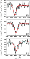 |
Fig. A.1. Spectra extracted from 2 pixel radius circles centered on the sources K1, K2, and K3, zoomed in on the NaID absorption line. The red line in each panel is the best-fit model of the NaID absorption features. |
where Iem is the normalization parameter, λK and λH are the wavelengths of sodium at respectively 5891 Å and 5896 Å, Cf is the covering factor, τ0 is the optical depth at the central λ, b is the Doppler parameter, and c is the speed of light. This model is widely used in literature (e.g., Rupke et al. 2005; Sato et al. 2009; Perna et al. 2020) and provides a physically motivated description of the absorption features, which can be used to derive column density and mass of the absorbing gas (Travascio et al. in prep.). The redshift estimated in this way for the sources K1 and K3, are consistent with those derived through molecular transitions with ALMA by B19.
All Tables
Properties of the ionized (Hα, [O III]; top subtable) and molecular (CO (3–2); bottom subtable in B19) outflows in PDS 456.
All Figures
|
Fig. 1. RGB wide filter images of the WFM (left) and NFM (right) MUSE datacube, obtained by collapsing the MUSE datacube in the same spectral regions as the HST/ACS-HCR filters F475W, F625W, and F775W for the WFM data, and F459M, F660N, and F892N for the NFM data. For the NFM data, spectral regions contaminated by instrument features fallen in the filters are excluded. In the WFM image the region studied in this work is highlighted, including PDS 456 and companions, with a dashed white box measuring 80 × 60 kpc2. The cyan box indicates the size (≈23 × 23 kpc2) of the NFM FOV centered on PDS 456. The positions of the nucleus of PDS 456 are indicated with black crosses. |
| In the text | |
|
Fig. 2. Extended emission surrounding PDS 456, within the region of the WFM-MUSE FoV indicated by a dashed white box in the left panel of Fig. 1. This RGB composite image is generated from the following images: optimally extracted narrowband images of Hα (R) and [O III]λ5008 Å (B) obtained using the CubEx tool, and the white-light image (WLI; G). The black cross symbols indicate the line-emitting companions detected with the Keck Telescope (Yun et al. 2004), ALMA Bischetti19, and in this work with MUSE (see Table 1 for details). MUSE continuum sources are visible in green. The white contours show the surface brightness levels of the [O III] nebula at 10, 50, 100, and 500 10−18 erg s−1 cm−2 arcsec−2. |
| In the text | |
|
Fig. 3. BPT diagram derived from spectral fit results for galaxy companions of PDS 456. The top panel displays the spectra and their best-fit models, while the bottom panel presents the [N II] -BPT diagram, for the galaxy companions of PDS 456. These spectra were extracted from circular regions with a radius of 2 pixels in the datacube, where the nuclear and continuum emission components of PDS 456 have been subtracted. The transparent gray dots show the values from the SDSS survey (credits: Jake Vanderplas & AstroML Developers). The black lines dividing different types of emissions in the BPT diagram are from Kewley et al. (2001). |
| In the text | |
|
Fig. 4. Maps of the extinction-corrected mass estimated from the Hα (top) and [O III] (bottom) emission, divided into Voronoi regions derived to reach a S/N > 3 of the Hβ line emission. The black thick contours in each map represent the S/N levels at 3, 5, 10, 30, and 50 of the [O III] line emission. The black cross gives the position of PDS 456. |
| In the text | |
|
Fig. 5. Total observed [O III] luminosity (L[O III]) of PDS 456 (red star) compared with that measured for other samples of Type 1 quasars in the redshift range z ∼ 0.1 to ∼4. The quasars at z < 1 are from Husemann et al. (2013; green dots), Husemann et al. (2014; yellow dots), Liu et al. (2014; purple dots), and Perna et al. (2017; orange dots). Quasars at z > 1 are from Coatman et al. (2019; blue dots) and Bischetti et al. (2017; red dots). |
| In the text | |
|
Fig. 6. Maps of w80 (top left), v50 (top right), v10 (bottom left), and v90 (bottom right) of the [O III] emission line. These maps provide an overview of the widths and velocity shifts from the entire [O III] profile. In each panel, the black thin contours represent the S/N levels shown in Fig. 4. The black thick contours in the center of the figure depict the molecular outflow, detected in B19. These contours correspond to the emission levels of 1, 4, 8, and 10 mJy. The white cross gives the position of the quasar. The white lines in each map represent 2σ Gaussian-smoothed contours that enclose the regions where w80 exceeds 400 km s−1. |
| In the text | |
|
Fig. 7. MUSE NFM surface brightness map of the Hα emission. The black contours show the S/N levels of the Hα emission of 3, 5, and 10. The gray contours show the morphology of the blueshifted CO (3–2) molecular outflow (B19), at the emission levels of 1, 4, 8, and 10 mJy. The black circles indicate regions affected by significant residuals in the PSF subtraction due to the quasar and a nearby continuum source. |
| In the text | |
|
Fig. 8. First (top) and second (bottom) moment of the flux distribution of the Hα emission obtained with the Cube2Im function in CubExtractor, representing the vshift and σvel maps. The gray contours show the morphology of the extended (up to ≈5 kpc) blueshifted CO (3–2) molecular outflow, detected by B19, at the emission levels of 1, 4, 8, and 10 mJy. The black circles and contours are the same as in Fig. 7. |
| In the text | |
|
Fig. 9. Spectra extracted from nuclear- and continuum-subtracted MUSE WFM (red; Hα) and NFM (black; Hα) datacubes, and from the ALMA data (green; CO (3–2)), in the region where the Hα outflow is observed in NFM MUSE data. |
| In the text | |
|
Fig. 10. Emission-line ratio maps for the extended gas around PDS 456. Top panel: [N II]/Hα emission line ratio map, at S/NHα > 2.5, whose pixel size is five times larger than the native pixel in NFM MUSE data, which corresponds to ∼1.3 FWHMPSF. The black dot gives the position of the central quasar, and has the FWHM size of the PSFNFM. Bottom panel: Map of the [O III]/Hβ line ratio estimated through the [O III] and Hβ optimally extracted NB images extracted from the WFM MUSE data with CubExtractor. The black contours represent the S/N levels of the Hα emission extracted from the NFM MUSE data at 3, 5, and 10. |
| In the text | |
|
Fig. 11. Spectra, in velocity units, extracted from the regions where the outflow dominates the emission (see text for details), in WFM (top panel) and NFM (bottom panel) MUSE data. Shown are a zoomed-in images of the [O III] (top panel) and Hα (bottom panel) transitions. The red lines show the best-fit model consisting of the combination of two Gaussian components: a narrow one (green) and a broader one (blue), tracing the outflow. |
| In the text | |
|
Fig. 12. vmax (top panel), Ṁout (central panel), and Ėkin (bottom panel) of the molecular and ionized outflow in PDS 456 (star symbols) vs. Lbol. We compare these values with those of ionized and molecular outflows reported in F17, B19, Fluetsch et al. (2019), and Speranza et al. (2024). For the estimation of the ionized outflow properties, an ne of 200 cm−3 from F17 was used. |
| In the text | |
|
Fig. A.1. Spectra extracted from 2 pixel radius circles centered on the sources K1, K2, and K3, zoomed in on the NaID absorption line. The red line in each panel is the best-fit model of the NaID absorption features. |
| In the text | |
Current usage metrics show cumulative count of Article Views (full-text article views including HTML views, PDF and ePub downloads, according to the available data) and Abstracts Views on Vision4Press platform.
Data correspond to usage on the plateform after 2015. The current usage metrics is available 48-96 hours after online publication and is updated daily on week days.
Initial download of the metrics may take a while.