| Issue |
A&A
Volume 691, November 2024
|
|
|---|---|---|
| Article Number | A346 | |
| Number of page(s) | 9 | |
| Section | Interstellar and circumstellar matter | |
| DOI | https://doi.org/10.1051/0004-6361/202450208 | |
| Published online | 26 November 2024 | |
Outflow from the very massive Wolf-Rayet binary Melnick 34★
1
Leibniz-Institut für Astrophysik Potsdam (AIP),
An der Sternwarte 16,
14482
Potsdam,
Germany
2
Institut für Astrophysik, Georg-August-Universität,
Friedrich-Hund-Platz 1,
37077
Göttingen,
Germany
3
Department of Physics & Astronomy, University of Sheffield,
Hounsfield Road,
Sheffield
S3 7RH,
UK
4
Leiden Observatory, Leiden University,
PO Box 9513,
2300 RA
Leiden,
The Netherlands
5
Instituto de Astrofísica e Ciências do Espaço, Universidade do Porto, CAUP,
Rua das Estrelas,
4150-762
Porto,
Portugal
★★ Corresponding author; This email address is being protected from spambots. You need JavaScript enabled to view it.
Received:
2
April
2024
Accepted:
10
October
2024
Abstract
Melnick 34 (Mk 34) is one of the most massive binary systems known and is one of the brightest X-ray point sources in the 30 Doradus region. We investigated the impact of this massive system on the surrounding interstellar medium (ISM) using the optical spectroscopic capabilities of the narrow-field mode (NFM) of the Multi-Unit Spectroscopic Explorer (MUSE). MUSE-NFM spatially resolved the ISM in the vicinity of Mk34 with a resolution comparable to that of the HST. The analysis of the [NII] λ 6583 and [SII] λ 6717 emission lines reveals a cone-like structure apparently originating from Mk 34 and extending southeast. Electron density maps and radial velocity measurements of the ISM lines further support an outflow scenario traced by these emissions. While no clear northwestern counterpart to this outflow was observed, we note increased extinction in that direction, towards the R136 cluster. The ISM material along the projected diagonal of the outflow on both sides of Mk 34 shows similar properties in terms of the emission line ratios seen in the Baldwin-Phillips-Terlevich diagram. These results are consistent across two observational epochs. Additionally, we examined the residual maps within a 0.5″ radius of Mk 34 after modeling and subtracting the point spread function. The observed variations in the residuals could potentially be linked to Mk 34’s known periodic behavior. However, further observations with appropriate cadence are needed to fully monitor the 155 day periodicity of Mk 34’s X-ray emissions.
Key words: stars: early-type / stars: jets / stars: kinematics and dynamics / stars: individual: Mk34 / ISM: jets and outflows
Based on observations made with ESO telescopes at the Paranal observatory under programmes 60.A-9351, 0104.D-0084 and 0104.D-0084.
© The Authors 2024
 Open Access article, published by EDP Sciences, under the terms of the Creative Commons Attribution License (https://creativecommons.org/licenses/by/4.0), which permits unrestricted use, distribution, and reproduction in any medium, provided the original work is properly cited.
This article is published in open access under the Subscribe to Open model. This email address is being protected from spambots. You need JavaScript enabled to view it. to support open access publication.
1 Introduction
Very massive stars (>100 M⊙) are rare in the Universe (Vink et al. 2015). However, massive OB stars are one of the main energy drivers and sources of processed chemical elements in the interstellar medium (ISM), and they chemically and dynamically shape the galaxies. Massive stars are also the most plausible sources of the ionization of the early Universe (Eldridge & Stanway 2022). Their strong stellar winds and outflows can punch holes in the ISM, through which ionizing radiation leaks (Weilbacher et al. 2018; Ramambason et al. 2020). The evolution of very massive stars and their interplay with the ISM must first be understood in our local neighborhood so that we may obtain a clearer view of the related phenomena at higher redshifts (Micheva et al. 2017) and in the early stages of the Universe.
The heart of the Tarantula nebula, NGC 2070, in the Large Magellanic Cloud (LMC) hosts the most massive stars known that have been spatially resolved (Crowther et al. 2010). The distance to the LMC of 49.9 kpc (Pietrzyński et al. 2013) means that we can study them individually and together with the ISM, allowing us to explore the stellar feedback from very massive stars in the surrounding medium. Melnick 34 (also known as Mk 34, BAT99 116, and Brey 84) is one of the most luminous Wolf-Rayet (WR) stars in NGC 2070 and is the main X-ray source (Crowther et al. 2022) after the core of the nebula itself, WR R136a1 (Doran et al. 2013). Mk 34 was initially classified as a single WN5h (Crowther & Dessart 1998) and subsequently as a WN5h:a (Schnurr et al. 2008; Crowther & Walborn 2011). It was claimed to have an initial record mass of 390 M⊙ (Hainich et al. 2014). Further multi-epoch studies showed a more complex picture, wherein Mk 34 is actually a highly eccentric binary of two very massive stars (Chené et al. 2011). The duplicity of Mk 34 was confirmed by the strong X-ray emission, likely induced by the colliding winds (Townsley et al. 2006). Follow-up observations in X-rays revealed a periodic variability of 155 days and an average luminosity that is one order of magnitude higher than that of any comparable WR binary in the Milky Way (Pollock et al. 2018) and ~23% higher than that of η Carinae. Additional optical parameters confirm that Mk 34 is a spectroscopic binary of two similar WN5h stars (Tehrani et al. 2019), which may end its life as a double black hole system (Belczynski et al. 2022).
Mk 34 is apparently in relative isolation from other bright stars (Castro et al. 2018), and is far enough from the core of the cluster (10″, 2.4 pc) to be individually resolved. It is a perfect laboratory in which to explore the feedback mechanisms of very massive stars in the surrounding medium. We spectro-scopically and spatially mapped Mk 34 using the state-of-the-art integral field spectrograph of Multi-Unit Spectroscopic Explorer (MUSE; Bacon et al. 2014; Roth et al. 2019) at the Very Large Telescope. MUSE in its narrow-field-mode configuration (NFM) allowed us to explore Mk 34 and the surrounding ISM (field of view of 7.5″ × 7.5″, 1.8 × 1.8 pc) from a ground-based telescope but with a spatial resolution similar to that of the Hubble Space Telescope (Castro et al. 2021b).
In the present study, we report the detection of apparent outflow signatures close to the Mk 34 binary system and imprints in the ISM using high-spatial-resolution optical spectroscopic data obtained with MUSE. After detailing the data used in this work in Sect. 2, we present the properties of the ISM surrounding Mk 34 in Sect. 3. In Sect. 4, we compare the results obtained across two available epochs. We model the point spread function of MUSE-NFM in Sect. 5 and examine the residual maps for evidence of possible outflows in the proximity of the binary. In Sect. 6, we explore the Baldwin-Phillips-Terlevich (BPT) diagram in the region around the Mk 34 outflow, searching for varying ionizing sources within the ISM to help trace and confirm this phenomenon. Finally, in Sect. 7, we present a discussion of the findings of this study and outline potential future directions to continue this work.
2 Data
Mk 34 MUSE-NFM data were obtained as part of the ESO observing programs 0104.D-0084 and 108.224L (PI N. Castro), which focused on spectroscopically resolving the core of NGC 2070, the R136 cluster (Castro et al. 2021b). The MUSE instrument (Bacon et al. 2014, 2010), mounted on the Very Large Telescope in Chile, in its NFM configuration offers a field of view of 7.5″×7.5″ and a pixel scale of 0.025″. The spectral information in each pixel spans 4800–9300 Å, with a resolving power of R ~ 3000 around Hα.
The field centered in Mk 34 was first observed on 25 November 2019. Under the weather conditions of that night (photometric sky with ambient seeing between 0.57″ and 0.83″), and with the performance of the adaptive optics, we achieved an image quality of ≈80 mas. The field was observed for a total exposure time of 2520 seconds. The integration time was split into four 630 s exposures, applying small spatial dithers (up to 0.1″) between each of them. A second epoch was observed on 9 December 2021 in clear conditions (and ambient seeing of 0.4″ to 0.58″), with identical exposure times, but this time with field rotations of 90° between each exposure to better suppress systematic errors. The combined cube of the Mk 34 field delivers a central AO-corrected peak with an FWHM of ≈65 mas in the I-band; however, the Strehl ratio is low and the overall point spread function is best described by a diffraction-limited Moffat-like core and a halo of uncorrected seeing (Fétick et al. 2019).
The MUSE-NFM data were reduced with the MUSE pipeline (Weilbacher et al. 2020) and included most of the standard processing steps. The basic processing, including CCD-level calibrations, such as bias correction, flat-fielding, wave-length calibration, geometrical calibration, illumination correction, and smoothed spatial twilight-flat correction, was carried out with v2.8 of the pipeline within the MuseWise (Vriend 2015) environment. The resulting “pixel tables” were extracted from the database and the post-processing steps were then carried out with v2.8.1 called from EsoRex. In NFM, the atmospheric refraction is normally corrected by the hardware dispersion corrector, but due to the high zenith distances of the observations (airmass 1.4 to 1.5), significant residuals (up to 60 mas) were visible. We therefore implemented an empirical correction as a patch to the standard MUSE pipeline, whereby we first reconstructed a cube coarsely sampled in 10 Å wavelength steps, measured the centroid for a selected star in each of them, and computed a fourth-order polynomial for both spatial directions. This polynomial was applied to the coordinates in the pixel table of the exposure in reverse in order to correct the residual refraction. This extra procedure resulted in a correction to below the spatial MUSE sampling (≲25 mas). We continued to follow the standard processing steps: The data of each exposure were flux calibrated, corrected to barycentric velocity, and corrected for spatial distortion (relative astrometric calibration). To achieve an absolute astrometric correction, we measured the centroid of one star in each exposure (using IRAF imexamine1) and computed offsets relative to the ICRS coordinates of the Gaia DR2 tables (Lindegren et al. 2018). The offsets and all processed pixel tables were then used to reconstruct a final cube for the field around Mk 34, sampled at the standard MUSE NFM voxel size of 25.19 mas × 25.42 mas × 1.25 Å. We also reconstructed images of the field in different broad-band filters.
Additionally, we used in this work data in NGC 2070 obtained as part of the MUSE science verification and commissioning of the wide-field-mode (MUSE-WFM) configuration in 2014 (Bacon et al. 2014). MUSE-WFM provides a large field of view of 1′×1′, and a pixel scale of 0.2″, but with a lower spatial resolution. The mosaic of NGC 2070 obtained in 2014 (Castro et al. 2021a) reached an image quality of 1″. For details on the observations and our reduction of NGC2070 MUSE-WFM data, we refer to Castro et al. (2018, 2021a).
3 Searching for outflow fingerprints in the ISM
The ISM surrounding Mk 34 is inevitably influenced by the elevated ionizing spectrum of the massive binary system Mk 34. To investigate this impact, we mapped the [NII] λ6583 and [SII] λ6717 emission lines around Mk 34, searching for evidence of the influence of ionization on the ISM. We modeled both emission lines using a Gaussian function combined with a second-order polynomial. The polynomial component accounts for the continuum and the broad Hα stellar wind component near Mk 34. To enhance the signal-to-noise ratio, we averaged the flux within a ±2 spatial pixel (spaxel) range during the field mapping. The systematic velocity of NGC 2070 of 265 km s−1 (Castro et al. 2018) was taken into account before modeling the lines.
The emission from both ions shows a similar spatial distribution (Fig. 1), with filamentary structures that, in projection, appear to originate from Mk 34 and extend towards the south-eastern part of the field. These features suggest the presence of a plausible outflow originating from Mk 34. Due to the consistent spatial distribution of both lines, and to avoid redundant information, the [NII] λ 6583 map is primarily used as the reference for discussion throughout this work.
Additionally, we explore the electron density and the interstellar extinction maps around Mk 34. The electron density was built based on the [SII] λλ6717, 6731 ratio following the solution given for a three-level atom by McCall (1984) and assuming an electron temperature of T = 104 K (see also Castro et al. 2018). The interstellar extinction c(Hβ) was obtained from the Hα/Hβ ratio, assuming Case B recombination theory for ne = 100 cm−3 and T=104 K, that is, an intrinsic ratio of I(Hα)/I(Hβ) = 2.86 (Hummer & Storey 1987). We adopted a standard extinction law (Cardelli et al. 1989) with RV = 3.1 to ensure a direct comparison with previous results in NGC 2070 using MUSE-WFM (Castro et al. 2018).
The ISM electron density strongly marks the same [NII] and [SII] emission patterns, a cone structure apparently originating in Mk 34 (panel b in Fig. 2). We do not find a symmetric counterpart of this cone structure on the northwest side of the field.
However, the extinction map - retrieved using the ISM Hα and Hβ emission lines (panel a in Fig. 2) – reveals higher values in the northwest toward the center of the cluster. The larger extinction could partially obscure any possible counterpart of the [NII] contribution. Additionally, the presence of the massive cluster R136 can also make it harder for any outflow to propagate toward it. A projected outflow would find an easier escape route moving away from R136, similar to our [NII] detection. An analog to this scenario at a larger scale may be the outflows detected in the candidate Lyman continuum emitter Mrk 71/NGC 2366 (Micheva et al. 2019).
The [NII] intensity map shows a narrow flow of material likely ejected from Mk34 at a projected distance of 0.89 pc from the binary. Nevertheless, the emission close to the east edge of the MUSE-NFM field of view also suggests that the pattern is more complex. [NII] intensity maps obtained with previous MUSE works (Castro et al. 2018) did not reach the spatial resolution of MUSE-NFM, but provide a larger view of the nitrogen emission map. Figure 3 combines both observing modes of MUSE, WFM, and NFM, and shows a more complex scenario. We cannot discard the composition of different clouds in the final projected image. Nonetheless, the focus of the [NII] emission around Mk 34 is remarkable and points to the binary system Mk 34 as the plausible source.
Figure 4 displays the radial velocity map of [NII] overlaid on the overall view provided by the MUSE-WFM, as shown in Fig. 3. The filament, traced by [NII], is redshifted with respect to the systemic velocity of NGC 2070, moving away from us in the southeast part of Mk 34. We measure a projected velocity of approximately 30 km s−1 in the peak of the [NII] velocity map.
A counterpart of blueshifted material is spotted on the west side of the image reaching velocities of a similar order (−40 km s−1).
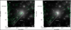 |
Fig. 1 Emission line maps within the field of view of MUSE-NFM (approximately 7.5″×7.5″) around Mk 34. Panel a: [NII] λ 6583 emission line map. Panel b: [SII] λ 6717 emission line map. We use the same intensity contours in both maps: contours range from 6 × 10⁻¹⁹ to 2 × 10⁻¹⁸ in steps of 2 × 10⁻¹⁹ erg s−1 cm−2 per spaxel. The MUSE-NFM image in the Johnson V band is shown in the background of both panels. |
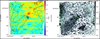 |
Fig. 2 Reddening coefficient c(Hβ) (left panel) and electron density (right panel) maps. Both panels display the emission distribution of [NII] λ6583 (green contours) described in Fig. 1 as a reference and, marking the proposed direction of the main outflow in Mk 34. The distance to the center of NGC 2070, the cluster R136, is marked in panel a. |
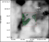 |
Fig. 3 [NII] λ 6583 emission mapped by MUSE-WFM (Castro et al. 2018) around Mk 34 with a spatial resolution of approximately 1″. The [NII] λ6583 emission mapped by MUSE-NFM is overplotted in green contours (see Fig. 1). The MUSE-NFM data sample the emission with a spatial resolution of approximately 80 mas and a field of view of 7.5"×7.5" (red square). The cluster R136 is indicated toward the north-west side of the field. |
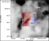 |
Fig. 4 [NII] λ 6583 emission mapped as described in Fig. 3. The [NII] radial velocity mapped by MUSE-NFM is overplotted in red and blue contours. Contours range from −30 km s−1 (blue) to 30 km s−1 (red) in steps of 10 km s−1 (NGC 2070 systemic velocity has been subtracted). See Fig. 3 as a reference for the additional labels. |
4 Revisiting Mk 34 and exploring variability
Mk 34 was observed again in December 2021, with a time interval of 745 days between the two epochs. The [NII] λ 6583 and [SII] λ 6717 intensity maps in 2021 display the same outflow pattern as in 2019. The electron density and extinction maps also support the same previous findings, a cone-like structure apparently emerging from Mk 34 in the southeast and more significant extinction in the northwest part toward the center of NGC 2070 (see Fig. 5). Fainter [NII] contours are drawn in the extinction map in Fig. 5, highlighting the correlation between higher extinction and the lack of an [NII] emission counterpart in the northwest side of Mk 34.
The difference between the two observing epochs shows a systematic flux discrepancy between all the sources in the field. We attribute this to an issue in the flux calibration. Before comparing the two epochs, it is necessary to put the fluxes and positions of the stars in a mutual reference system. We use the objects detected by the Gaia (Lindegren et al. 2018) survey around Mk 34 as calibration anchors within the MUSE-NFM field of view, finding ten stars in total. First, we checked the positions in both data sets and found variations of less than 0.5 pixels on average. Based on this result, we conclude that a correction in the astrometry is not needed (Fig. 5). Second, we measured the continuum flux around [NII] λ 6583 for the ten targets and find that we need a systematic correction of 1.15 in the flux to place the fluxes of the ten reference sources in the two epochs into the same reference system. Within several arcseconds around Mk 34, we do not detect significant quantitative differences between the two epochs (Fig. 6). A closer examination of Mk 34 at a scale of less than 1″, using the continuum flux around the [NII] λ 6583 emission line, reveals differences that may be associated with short-term events occurring very close to the star. Moreover, the difference between the two images highlights a diagonal pattern, extending from southeast to northwest (marked in Fig. 6), which aligns with the proposed [NII] and [SII] outflow maps.
Figure 7 illustrates the differences between the two epochs for the properties analyzed in this study. The intensity of the [NII] λ 6583 line shows stronger emission in 2019 around Mk 34 and along the ISM outflow path compared to the 2021 data. The electron density and extinction exhibit significant changes primarily in the region closer to Mk 34. We observed substantial differences in density at the location of Mk 34, with the electron density in 2019 being significantly higher than in 2021. However, we must approach these large values with caution, as the three-level atom solution provided by McCall (1984) may not be applicable in the environment surrounding a massive and hot binary system like Mk 34. Additionally, assuming an electron temperature of T = 104 K near Mk 34 may be unrealistic. The final panel in Fig. 7 does not reveal any clear pattern in the [NII] λ 6583 radial velocities between the two epochs, aside from a few small features near the binary system. These velocity measurements could be influenced by the significant Hα contribution.
5 Modeling and extraction of the point spread function
We analyzed the residuals of the point spread function (PSF) beneath the strong flux profile of Mk 34 in the MUSE data to explore the intense activity of the binary system within 0.5″ and to investigate potential the links to ISM emissions. Additionally, we examined how small-scale variations might be influenced by the effects of the AO-corrected PSF. The PSF of Mk 34 was modeled and subtracted at each wavelength of the datacube individually for both epochs. The modeling was performed using the MAOPPY (Modelization of the Adaptive Optics PSF in Python) library2, which is specifically designed for modeling PSFs in adaptive optics(AO)-assisted observations. The MAOPPY models have been tested on MUSE data taken in AO narrow-field mode, achieving a relative error of less than 1% for both simulated and experimental data (Fétick et al. 2019).
The total PSF residual in 2019, obtained after adding all the layers in the datacube, shows four main contributions around the core of Mk 34, where the PSF model fit by MAOPPY under-subtracts the data. In contrast, in the central part and the region around these four points, the model produces a negative residual (Fig. 8). This negative feature resembles the residual maps reported by Fétick et al. (2019) as part of their characterization of the MUSE-NFM PSF. The PSF residual in 2021 displays a similar average pattern to that in 2019; however, the details in the core change. The four contributions are replaced by two positive regions, primarily along the east-west axis of Mk 34. It is worth mentioning here again that the 2021 data were obtained with four rotation settings (see Sect. 2), which could influence the differences observed between the two epochs.
Figure 8 also displays the residual at the wavelength of [NII] λ 6583 after accounting for the systemic velocity of NGC 2070. The outflow described in Sect. 3 is visible in both epochs. Only the PSF of Mk 34 was modeled and subtracted in the present work. The remaining fainter stars, which are still visible in Fig. 8, were not included in this exercise.
We do not find a clear connection between the PSF residuals near Mk 34 and the ISM outflow. Although the positive pattern observed in 2021 may align with the direction indicated by the [NII] and [SII] intensity maps, evidence from a single epoch is insufficient to draw a conclusion. The PSF was modeled for each wavelength individually, revealing very similar patterns across the entire MUSE datacube in the 2019 and 2021 datacubes. This consistency adds robustness to the maps shown in Fig. 8. We may be observing events near Mk 34 that vary over short periods and potentially relate to the 155 day period reported by Pollock et al. (2018). We tentatively hypothesize that we are witnessing material expelled as a result of interactions between these two very massive stars. While this scenario could be further explored with observations taken at the appropriate cadence, it cannot be confirmed with the current data.
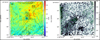 |
Fig. 5 Reddening coefficient c(Hβ) (left panel) and electron density (right panel) maps extracted from the 2021 epoch. In the left panel, the fainter contours of [NII] λ 6583 emission are delineated (from 2 × 10⁻¹⁹ to 2 × 10⁻¹⁸ erg s−1 cm−2 in increments of 2 × 10⁻¹⁹ erg s−1 cm−2 per spaxel) in comparison with the depiction in Fig. 1. This adjustment was made to accentuate the observed correlation between large c(Hβ) values and the absence of [NII] emission in the northwest of Mk 34. |
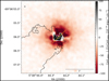 |
Fig. 6 Difference in the continuum flux around [NII] λ 6583 between the observations in 2019 and 2021. A factor of 1.15 was applied to the 2021 observations to correct for differences in the flux calibrations (see Sect. 4). The proposed flow direction is indicated by a solid orange line, along with the edges in the [NII] λ 6583 contours displayed in Figs. 1 and 5 to highlight the path within the ISM. |
6 Mapping the outflow regions using the BPT diagram
The BPT diagram is commonly employed to distinguish sources based on the nature of the ionizing origins, such as star-forming galaxies and active galactic nuclei (Baldwin et al. 1981), as well as to differentiate between shocks and photoionized gas (e.g., HII regions from planetary nebulae and supernova remnants; Micheva et al. 2022). We explored the emission-line ratios involved in the BPT diagram around Mk 34 (i.e., log10 ([NII]λ6583/Hα)) and log10 ([OIII]λ5007/Hβ)) using Voronoi binning to increase the signal-to-noise ratio.
To create diagnostic diagrams of the region around Mk34 we first fitted Hα with a single Gaussian in every spaxel of the MUSE cube and used its propagated noise to compute a S/N per pixel. This estimate was then used as input for the Voronoi binning (using the vorbin Python package, Cappellari & Copin 2003), which allowed us to create about 2200 bins of S /N ≈ 500 in the Hα line. To extract the line measurements, the spectra of the resulting bins were then separately fitted over two wavelength ranges (4800–5095Å, including Hβ and [OIII]λλ4959, 5007, and He Iλ5015, and 6520–6994Å, including [NII]λλ6548, 83, Ha, He Iλ6678, and [SII]λλ6716, 31) using a model of Gaussian peaks for the emission lines and a seventh-degree polynomial for the continuum. We used the pPXF (Cappellari 2017) package to carry out the line fitting. The fit leaves residuals in the spatial positions where the light is dominated by stars, especially around the Balmer lines, and we therefore mark these regions. Based on the maps of the line ratios [OIII]λ5007/Hβ and [NII]λ6583/Hα, we then manually defined regions of interest using polygon regions in the SAO DS9 viewer (Joye & Mandel 2003); these are used to color the points in the BPT diagrams. The background-subtracted point in the BPT diagram was created by interpolating over the red region that marks the spatial extent of the outflow. We used AstroPy’s interpolate_replace_nans function to determine the surrounding background in the map of each line, subtracted it, and then masked all non-positive bins. We then computed the BPT line ratios using the median flux left after subtraction. The error bars are the median absolute deviation of all subtracted bins within the red region.
log10 ([NII]λ6583/Hα) and log10 ([OIII]λ5007/Hβ) line ratios (see Fig. 9) highlight the outflow candidate presented in this work. We visually marked several regions in the line-ratio maps and checked their distribution in the BPT diagram. These areas are located in the regions expected to host strong star formation (Crowther et al. 2017), matching also the predicted position by numerical BPASS and CLOUDY simluations (Xiao et al. 2018). Additionally, they are located close to the position of the the so-called green pea galaxies (Cardamone et al. 2009), suggesting similar high-excitation properties. However, we find lower observed electron densities than those suggested by the best-fitting Xiao et al. (2018)’s simulations. This discrepancy in the electron density was also noted by Xiao et al. (2018), and was attributed in part to the effects of the depletion of metals onto interstellar dust grains.
Previous studies already highlighted the similarity in nebular properties of 30 Doradus and extreme star-forming galaxies, including green peas (Micheva et al. 2017; Monreal-Ibero et al. 2023). Although the regions are not completely separated in the BPT diagram, they are clustering, on average, at slightly different values of log10 ([NII]λ6583/Hα). The outflow (red area in Fig. 9) and the diametrically opposite region (purple area in Fig. 9) are located at similar values in the BPT diagram. Notably, this diametrically opposite region roughly corresponds to the blueshifted area shown in Fig. 4. The explored areas surrounding Mk 34 are systematically located below the average values reported in the extreme Lyman-continuum-emitting green pea galaxies (Micheva et al. 2017) in the BPT diagram (Fig. 10). Because the outflow consists of ionized gas that adds about 10% flux to the Hα surface brightness, we also aimed to subtract the surrounding ionized background to isolate the line ratios due to the outflow itself. This resulting background-corrected median flux is located in a very different region of the BPT diagram (red point in Fig. 10) where shock models are located. Specifically, the MAPPINGS III models (Allen et al. 2008), which include shock and precursor, cover exactly this area for LMC metallicity, 200 ≲ V ≲ 250 km/s, and 1 ≲ B ≲ 5 µG. We see this as an indication that the outflow from Mk 34 induces shocks in the surrounding ISM.
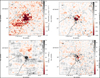 |
Fig. 7 Comparison of emission and physical properties between the 2019 and 2021 epochs. Panel a: differences in [NII] λ 6583 between the two epochs. Panel b: difference in electron density measured in 2019 and 2021. Panel c: difference in extinction measured in 2019 and 2021. Panel d: difference in [NII] λ 6583 radial velocities measured in 2019 and 2021. The path of [NII] λ 6583 intensity is highlighted by the edges in the [NII] λ 6583 contours displayed in Figs. 1 and 5, marking the detection within the ISM across all four panels. |
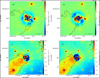 |
Fig. 8 PSF residual maps. Panel a: total PSF residual in 2019. Panel b: total PSF residual in 2021. Panel c: PSF residual in 2019 at the position of [NII] λ 6583. Panel d: PSF residual in 2021 at the position of [NII] λ 6583. The path of [NII] λ 6583 intensity is highlighted by the edges in the [NII] λ 6583 contours displayed in Figs. 1 and 5, marking the detection within the ISM across all four panels. |
7 Discussion and future steps
Reported outflows in massive objects are scarce and are mainly detected at radio wavelengths (Carrasco-González et al. 2010). Several detections have also been reported at optical and IR wavelengths in stellar nurseries, where stellar sources are still deeply buried in the molecular cloud (Caratti o Garatti et al. 2015; McLeod et al. 2018). Mk 34 is not a star in the formation phase. It is a system of two-core hydrogen-burning very massive stars, where the nursery cloud was swept away some time ago. The fact that the stellar sources and outflow can be studied separately makes this system an excellent target with which to empirically explore the origin of these ejections into the ISM. The colliding stellar winds in very massive systems can indeed generate outflows and eject processed material further into the ISM (Lebedev & Myasnikov 1990; Lamberts et al. 2012). The high spatial resolution of MUSE-NFM confirms the impact of outflow in the ISM, opening channels for the ionizing radiation to escape (Ramambason et al. 2020; Rosen & Krumholz 2020), as shown in Fig. 3.
The maps defined by the [NII] and [SII] emission lines reveal a cone-like structure originating from Mk 34, suggesting a plausible outflow. This finding is also confirmed by the electron density and ISM radial velocity maps around Mk 34. The ISM material appears to propagate toward the southeast region of Mk 34, with no clear counterpart observed in the northwest of the system. However, along the direction marked by the [NII] and [SII] filaments, the material exhibits similar properties on both sides of Mk 34, as indicated by the emission-line ratios in the BPT diagram. We detect greater extinction on the northwest side of Mk 34, which correlates with the lack of [NII] emission and may explain the absence of a corresponding outflow in that direction.
These ISM characteristics were consistently observed across both epochs. Between the 2019 and 2021 observations, we noted changes primarily in the intensity maps, as well as in the electron density and extinction within a 0.5″ radius of Mk 34, indicating possible monthly variations in the system. Transient phenomena, such as the formation and dissipation of emission disks, are not uncommon and have been documented in several Oe/Be stars (Rivinius et al. 2013). A notable example is AzV493, a scarce Oe-type star in the Small Magellanic Cloud (SMC), which exhibits significant spectroscopic variations dominated by a 14.6 year cycle, along with intense photometric fluctuations on shorter timescales (months) and approximately 40 day oscillations (Oey et al. 2023). The variability pattern observed in Mk 34 aligns with the expected behavior of massive, dynamically active systems of this kind.
We modeled and subtracted the Mk34 MUSE-NFM PSF to search for additional signals close to the star. The 2019 PSF residual map reveals several positive regions near Mk34 within a circle of 0.5″ in radius centered on the system. This pattern is consistently observed in the individual analysis of each wavelength, providing robust results. The possibility that we are witnessing bursts originating from the system is intriguing and not entirely unexpected. The collision of the supersonic stellar winds produced by the twin WRs in Mk 34 could result in rapid outflows (Lebedev & Myasnikov 1990; Lamberts et al. 2012). However, we must exercise caution and seek additional observations to further investigate this phenomenon. The change in the pattern observed in 2021 once again highlights the need for further observations in future epochs.
MUSE-NFM has the capability of spectroscopically mapping the impact of the feedback from the most massive stars on the surrounding ISM, and couldbe usedto examine thecontribution of this feedback to the ionization and chemical composition of the cluster. The present work conducted on Mk 34 is a demonstration of these capabilities, with MUSE-NFM achieving a spatial resolution of ≈80 mas in both epochs. The detection of the [NII] and [SII] filaments originating from Mk 34 suggests we that it may be possible to develop a better observational characterization of the dense and extensive stellar winds of Mk 34 and binary interactions. Numerical radiation-hydrodynamic modeling of the stellar winds of massive stars shows that time-dependent wind develops a very inhomogeneous clumped structure (Owocki et al. 1988; Sundqvist et al. 2018). The current state-of-the-art high-spatial-resolution spectrographs are excellent instruments with which to explore the extended stellar winds of the most massive stars known and to record their development over time. Comprehensively understanding dynamic events such as those observed in Mk 34 requires supplementary data that enable continuous monitoring. Additional observations of Mk 34 will be requested to investigate short-term variations that cannot be adequately mapped with the two epochs separated by 745 days in the present work, and to explore a potential correlation with the 155 day period of the Mk 34 binary system.
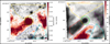 |
Fig. 9 Emission line ratios Hβ/[OIII]λ 5007 and Hα/[NII]λ 6583 are shown on the left and right panels, respectively. We visually identified several areas to explore their position and nature in the BPT diagram (Baldwin et al. 1981) (colored regions in both panels). |
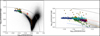 |
Fig. 10 Distribution of the areas highlighted in Fig. 9 in the BPT diagram (Baldwin et al. 1981). The colored dots follow the color coding used in Fig. 9; the large red point represents the background-subtracted line ratios of the red region. The right panel zooms into the more general view displayed on the left. The BPT diagram extracted from the SDSS DR7 sample (Abazajian et al. 2009) is displayed in the background (gray shaded area) as a reference, together with the Kewley et al. (2001) maximum starburst line in both panels. Extreme Lyman-continuum-emitting green pea galaxies (orange diamonds), updated from Micheva et al. (2017), are also shown. Additionally, the observed regions are compared with numerical predictions using BPASS and CLOUDY (Xiao et al. 2018). The simulations were calculated using the Large Magellanic Cloud metallicity, an age of 1 Myr, and a hydrogen density log10 (nH[cm−3]) ranging between 2 (dotted-dashed blue line), 2.5 (dotted-dashed orange line), and 3 (dashed red line). |
Acknowledgements
The authors thanks the referee for useful comments and helpful suggestions that improved this manuscript. NC acknowledges funding from the Deutsche Forschungsgemeinschaft (DFG) – CA 2551/1-1,2 and BMBF ErUM (project VLTBlueMUSE, grant 05A23MGA). PMW received support from BMBF ErUM (VLT-BlueMUSE and BlueMUSE-CD, grants 05A20BAB and 05A23BAC). Our research used Astropy, a community-developed core Pythonpackage for Astronomy (Astropy Collaboration 2013), and APLpy, an open-source plotting package for Python (Robitaille & Bressert 2012).
References
- Abazajian, K. N., Adelman-McCarthy, J. K., Agüeros, M. A., et al. 2009, ApJS, 182, 543 [Google Scholar]
- Allen, M. G., Groves, B. A., Dopita, M. A., Sutherland, R. S., & Kewley, L. J. 2008, ApJS, 178, 20 [Google Scholar]
- Astropy Collaboration (Robitaille, T. P., et al.) 2013, A&A, 558, A33 [NASA ADS] [CrossRef] [EDP Sciences] [Google Scholar]
- Bacon, R., Accardo, M., Adjali, L., et al. 2010, SPIE Conf. Ser., 7735, 773508 [Google Scholar]
- Bacon, R., Vernet, J., Borisova, E., et al. 2014, The Messenger, 157, 13 [NASA ADS] [Google Scholar]
- Baldwin, J. A., Phillips, M. M., & Terlevich, R. 1981, PASP, 93, 5 [Google Scholar]
- Belczynski, K., Romagnolo, A., Olejak, A., et al. 2022, ApJ, 925, 69 [NASA ADS] [CrossRef] [Google Scholar]
- Cappellari, M. 2017, MNRAS, 466, 798 [Google Scholar]
- Cappellari, M., & Copin, Y. 2003, MNRAS, 342, 345 [Google Scholar]
- Caratti o Garatti, A., Stecklum, B., Linz, H., Garcia Lopez, R., & Sanna, A. 2015, A&A, 573, A82 [NASA ADS] [CrossRef] [EDP Sciences] [Google Scholar]
- Cardamone, C., Schawinski, K., Sarzi, M., et al. 2009, MNRAS, 399, 1191 [NASA ADS] [CrossRef] [Google Scholar]
- Cardelli, J. A., Clayton, G. C., & Mathis, J. S. 1989, ApJ, 345, 245 [Google Scholar]
- Carrasco-González, C., Rodríguez, L. F., Anglada, G., et al. 2010, Science, 330, 1209 [CrossRef] [Google Scholar]
- Castro, N., Crowther, P. A., Evans, C. J., et al. 2018, A&A, 614, A147 [NASA ADS] [CrossRef] [EDP Sciences] [Google Scholar]
- Castro, N., Crowther, P. A., Evans, C. J., et al. 2021a, A&A, 648, A65 [NASA ADS] [CrossRef] [EDP Sciences] [Google Scholar]
- Castro, N., Roth, M. M., Weilbacher, P. M., et al. 2021b, The Messenger, 182, 50 [Google Scholar]
- Chené, A.-N., Schnurr, O., Crowther, P. A., Fernández-Lajús, E., & Moffat, A. F. J. 2011, in Active OB Stars: Structure, Evolution, Mass Loss, and Critical Limits, 272, eds. C. Neiner, G. Wade, G. Meynet, & G. Peters, 497 [Google Scholar]
- Crowther, P. A., & Dessart, L. 1998, MNRAS, 296, 622 [NASA ADS] [CrossRef] [Google Scholar]
- Crowther, P. A., & Walborn, N. R. 2011, MNRAS, 416, 1311 [Google Scholar]
- Crowther, P. A., Schnurr, O., Hirschi, R., et al. 2010, MNRAS, 408, 731 [Google Scholar]
- Crowther, P. A., Castro, N., Evans, C. J., et al. 2017, The Messenger, 170, 40 [Google Scholar]
- Crowther, P. A., Broos, P. S., Townsley, L. K., et al. 2022, MNRAS, 515, 4130 [NASA ADS] [CrossRef] [Google Scholar]
- Doran, E. I., Crowther, P. A., de Koter, A., et al. 2013, A&A, 558, A134 [NASA ADS] [CrossRef] [EDP Sciences] [Google Scholar]
- Eldridge, J. J., & Stanway, E. R. 2022, arXiv e-prints [arXiv:2202.01413] [Google Scholar]
- Fétick, R. J. L., Fusco, T., Neichel, B., et al. 2019, A&A, 628, A99 [NASA ADS] [CrossRef] [EDP Sciences] [Google Scholar]
- Hainich, R., Rühling, U., Todt, H., et al. 2014, A&A, 565, A27 [NASA ADS] [CrossRef] [EDP Sciences] [Google Scholar]
- Hummer, D. G., & Storey, P. J. 1987, MNRAS, 224, 801 [NASA ADS] [CrossRef] [Google Scholar]
- Joye, W. A., & Mandel, E. 2003, in Astronomical Society of the Pacific Conference Series, 295, Astronomical Data Analysis Software and Systems XII, eds. H. E. Payne, R. I. Jedrzejewski, & R. N. Hook, 489 [NASA ADS] [Google Scholar]
- Kewley, L. J., Dopita, M. A., Sutherland, R. S., Heisler, C. A., & Trevena, J. 2001, ApJ, 556, 121 [Google Scholar]
- Lamberts, A., Dubus, G., Lesur, G., & Fromang, S. 2012, A&A, 546, A60 [NASA ADS] [CrossRef] [EDP Sciences] [Google Scholar]
- Lebedev, M. G., & Myasnikov, A. V. 1990, Fluid Dyn., 25, 629 [Google Scholar]
- Lindegren, L., Hernández, J., Bombrun, A., et al. 2018, A&A, 616, A2 [NASA ADS] [CrossRef] [EDP Sciences] [Google Scholar]
- McCall, M. L. 1984, MNRAS, 208, 253 [NASA ADS] [CrossRef] [Google Scholar]
- McLeod, A. F., Reiter, M., Kuiper, R., Klaassen, P. D., & Evans, C. J. 2018, Nature, 554, 334 [CrossRef] [Google Scholar]
- Micheva, G., Oey, M. S., Jaskot, A. E., & James, B. L. 2017, AJ, 845, 165 [NASA ADS] [Google Scholar]
- Micheva, G., Christian Herenz, E., Roth, M. M., Östlin, G., & Girichidis, P. 2019, A&A, 623, A145 [NASA ADS] [CrossRef] [EDP Sciences] [Google Scholar]
- Micheva, G., Roth, M. M., Weilbacher, P. M., et al. 2022, A&A, 668, A74 [NASA ADS] [CrossRef] [EDP Sciences] [Google Scholar]
- Monreal-Ibero, A., Weilbacher, P. M., Micheva, G., Kollatschny, W., & Maseda, M. 2023, A&A, 674, A210 [NASA ADS] [CrossRef] [EDP Sciences] [Google Scholar]
- Oey, M. S., Castro, N., Renzo, M., et al. 2023, arXiv e-prints [arXiv:2301.11433] [Google Scholar]
- Owocki, S. P., Castor, J. I., & Rybicki, G. B. 1988, ApJ, 335, 914 [NASA ADS] [CrossRef] [Google Scholar]
- Pietrzyński, G., Graczyk, D., Gieren, W., et al. 2013, Nature, 495, 76 [Google Scholar]
- Pollock, A. M. T., Crowther, P. A., Tehrani, K., Broos, P. S., & Townsley, L. K. 2018, MNRAS, 474, 3228 [CrossRef] [Google Scholar]
- Ramambason, L., Schaerer, D., Stasinska, G., et al. 2020, A&A, 644, A21 [NASA ADS] [CrossRef] [EDP Sciences] [Google Scholar]
- Rivinius, T., Carciofi, A. C., & Martayan, C. 2013, A&A Rev., 21, 69 [NASA ADS] [CrossRef] [Google Scholar]
- Robitaille, T., & Bressert, E. 2012, APLpy: Astronomical Plotting Library in Python, Astrophysics Source Code Library [record ascl:1208.017] [Google Scholar]
- Rosen, A. L., & Krumholz, M. R. 2020, AJ, 160, 78 [NASA ADS] [CrossRef] [Google Scholar]
- Roth, M. M., Weilbacher, P. M., & Castro, N. 2019, Astron. Nachr., 340, 989 [Google Scholar]
- Schnurr, O., Moffat, A. F. J., St-Louis, N., Morrell, N. I., & Guerrero, M. A. 2008, MNRAS, 389, 806 [NASA ADS] [CrossRef] [Google Scholar]
- Sundqvist, J. O., Owocki, S. P., & Puls, J. 2018, A&A, 611, A17 [NASA ADS] [CrossRef] [EDP Sciences] [Google Scholar]
- Tehrani, K. A., Crowther, P. A., Bestenlehner, J. M., et al. 2019, MNRAS, 484, 2692 [NASA ADS] [CrossRef] [Google Scholar]
- Tody, D. 1993, in Astronomical Society of the Pacific Conference Series, 52, Astronomical Data Analysis Software and Systems II, eds. R. J. Hanisch, R. J. V. Brissenden, & J. Barnes, 173 [NASA ADS] [Google Scholar]
- Townsley, L. K., Broos, P. S., Feigelson, E. D., Garmire, G. P., & Getman, K. V. 2006, AJ, 131, 2164 [NASA ADS] [CrossRef] [Google Scholar]
- Vink, J. S., Heger, A., Krumholz, M. R., et al. 2015, Highlights Astron., 16, 51 [Google Scholar]
- Vriend, W.-J. 2015, in Science Operations 2015: Science Data Management – An ESO/ESA Workshop, 1 [Google Scholar]
- Weilbacher, P. M., Monreal-Ibero, A., Verhamme, A., et al. 2018, A&A, 611, A95 [NASA ADS] [CrossRef] [EDP Sciences] [Google Scholar]
- Weilbacher, P. M., Palsa, R., Streicher, O., et al. 2020, A&A, 641, A28 [NASA ADS] [CrossRef] [EDP Sciences] [Google Scholar]
- Xiao, L., Stanway, E. R., & Eldridge, J. J. 2018, MNRAS, 477, 904 [Google Scholar]
IRAF was developed by the National Optical Astronomy Observatory (Tody 1993) and has been maintained by the IRAF community since 2017 (https://iraf-community.github.io/).
All Figures
|
Fig. 1 Emission line maps within the field of view of MUSE-NFM (approximately 7.5″×7.5″) around Mk 34. Panel a: [NII] λ 6583 emission line map. Panel b: [SII] λ 6717 emission line map. We use the same intensity contours in both maps: contours range from 6 × 10⁻¹⁹ to 2 × 10⁻¹⁸ in steps of 2 × 10⁻¹⁹ erg s−1 cm−2 per spaxel. The MUSE-NFM image in the Johnson V band is shown in the background of both panels. |
| In the text | |
|
Fig. 2 Reddening coefficient c(Hβ) (left panel) and electron density (right panel) maps. Both panels display the emission distribution of [NII] λ6583 (green contours) described in Fig. 1 as a reference and, marking the proposed direction of the main outflow in Mk 34. The distance to the center of NGC 2070, the cluster R136, is marked in panel a. |
| In the text | |
|
Fig. 3 [NII] λ 6583 emission mapped by MUSE-WFM (Castro et al. 2018) around Mk 34 with a spatial resolution of approximately 1″. The [NII] λ6583 emission mapped by MUSE-NFM is overplotted in green contours (see Fig. 1). The MUSE-NFM data sample the emission with a spatial resolution of approximately 80 mas and a field of view of 7.5"×7.5" (red square). The cluster R136 is indicated toward the north-west side of the field. |
| In the text | |
|
Fig. 4 [NII] λ 6583 emission mapped as described in Fig. 3. The [NII] radial velocity mapped by MUSE-NFM is overplotted in red and blue contours. Contours range from −30 km s−1 (blue) to 30 km s−1 (red) in steps of 10 km s−1 (NGC 2070 systemic velocity has been subtracted). See Fig. 3 as a reference for the additional labels. |
| In the text | |
|
Fig. 5 Reddening coefficient c(Hβ) (left panel) and electron density (right panel) maps extracted from the 2021 epoch. In the left panel, the fainter contours of [NII] λ 6583 emission are delineated (from 2 × 10⁻¹⁹ to 2 × 10⁻¹⁸ erg s−1 cm−2 in increments of 2 × 10⁻¹⁹ erg s−1 cm−2 per spaxel) in comparison with the depiction in Fig. 1. This adjustment was made to accentuate the observed correlation between large c(Hβ) values and the absence of [NII] emission in the northwest of Mk 34. |
| In the text | |
|
Fig. 6 Difference in the continuum flux around [NII] λ 6583 between the observations in 2019 and 2021. A factor of 1.15 was applied to the 2021 observations to correct for differences in the flux calibrations (see Sect. 4). The proposed flow direction is indicated by a solid orange line, along with the edges in the [NII] λ 6583 contours displayed in Figs. 1 and 5 to highlight the path within the ISM. |
| In the text | |
|
Fig. 7 Comparison of emission and physical properties between the 2019 and 2021 epochs. Panel a: differences in [NII] λ 6583 between the two epochs. Panel b: difference in electron density measured in 2019 and 2021. Panel c: difference in extinction measured in 2019 and 2021. Panel d: difference in [NII] λ 6583 radial velocities measured in 2019 and 2021. The path of [NII] λ 6583 intensity is highlighted by the edges in the [NII] λ 6583 contours displayed in Figs. 1 and 5, marking the detection within the ISM across all four panels. |
| In the text | |
|
Fig. 8 PSF residual maps. Panel a: total PSF residual in 2019. Panel b: total PSF residual in 2021. Panel c: PSF residual in 2019 at the position of [NII] λ 6583. Panel d: PSF residual in 2021 at the position of [NII] λ 6583. The path of [NII] λ 6583 intensity is highlighted by the edges in the [NII] λ 6583 contours displayed in Figs. 1 and 5, marking the detection within the ISM across all four panels. |
| In the text | |
|
Fig. 9 Emission line ratios Hβ/[OIII]λ 5007 and Hα/[NII]λ 6583 are shown on the left and right panels, respectively. We visually identified several areas to explore their position and nature in the BPT diagram (Baldwin et al. 1981) (colored regions in both panels). |
| In the text | |
|
Fig. 10 Distribution of the areas highlighted in Fig. 9 in the BPT diagram (Baldwin et al. 1981). The colored dots follow the color coding used in Fig. 9; the large red point represents the background-subtracted line ratios of the red region. The right panel zooms into the more general view displayed on the left. The BPT diagram extracted from the SDSS DR7 sample (Abazajian et al. 2009) is displayed in the background (gray shaded area) as a reference, together with the Kewley et al. (2001) maximum starburst line in both panels. Extreme Lyman-continuum-emitting green pea galaxies (orange diamonds), updated from Micheva et al. (2017), are also shown. Additionally, the observed regions are compared with numerical predictions using BPASS and CLOUDY (Xiao et al. 2018). The simulations were calculated using the Large Magellanic Cloud metallicity, an age of 1 Myr, and a hydrogen density log10 (nH[cm−3]) ranging between 2 (dotted-dashed blue line), 2.5 (dotted-dashed orange line), and 3 (dashed red line). |
| In the text | |
Current usage metrics show cumulative count of Article Views (full-text article views including HTML views, PDF and ePub downloads, according to the available data) and Abstracts Views on Vision4Press platform.
Data correspond to usage on the plateform after 2015. The current usage metrics is available 48-96 hours after online publication and is updated daily on week days.
Initial download of the metrics may take a while.