The SRG/eROSITA All-Sky Survey

R. Seppi; J. Comparat; V. Ghirardini; C. Garrel; E. Artis; A. G. Sánchez; A. Liu; N. Clerc; E. Bulbul; S. Grandis; M. Kluge; T. H. Reiprich; A. Merloni; X. Zhang; Y. E. Bahar; S. Shreeram; J. Sanders; M. Ramos-Ceja; M. Krumpe

doi:10.1051/0004-6361/202348843

Home

All issues

Volume 686 (June 2024)

A&A, 686 (2024) A196

Full HTML

Open Access

Issue		A&A Volume 686, June 2024


Article Number		A196
Number of page(s)		20
Section		Cosmology (including clusters of galaxies)
DOI		https://doi.org/10.1051/0004-6361/202348843
Published online		12 June 2024

A&A, 686, A196 (2024)

Tracing the large-scale structure with a clustering study of galaxy clusters

R. Seppi¹^,2, J. Comparat¹, V. Ghirardini¹, C. Garrel¹, E. Artis¹, A. G. Sánchez¹, A. Liu¹, N. Clerc³, E. Bulbul¹, S. Grandis⁴, M. Kluge¹, T. H. Reiprich⁵, A. Merloni¹, X. Zhang¹, Y. E. Bahar¹, S. Shreeram¹, J. Sanders¹, M. Ramos-Ceja¹ and M. Krumpe⁶

¹ Max-Planck-Institut für Extraterrestrische Physik (MPE), Giessenbachstraße 1, 85748 Garching bei München, Germany
² Department of Astronomy, University of Geneva, Ch. d’Ecogia 16, 1290 Versoix, Switzerland
e-mail: riccardo.seppi@unige.ch
³ IRAP, Université de Toulouse, CNRS, UPS, CNES, Toulouse, France
⁴ Universität Innsbruck, Institut für Astro- und Teilchenphysik, Technikerstr. 25/8, 6020 Innsbruck, Austria
⁵ Argelander-Institut für Astronomie (AIfA), Universität Bonn, Auf dem Hügel 71, 53121 Bonn, Germany
⁶ Leibniz-Institut für Astrophysik Potsdam, An der Sternwarte 16, 14482 Potsdam, Germany

Received: 5 December 2023
Accepted: 20 March 2024

Abstract

Context. The spatial distribution of galaxy clusters provides a reliable tracer of the large-scale distribution of matter in the Universe. The clustering signal depends on intrinsic cluster properties and cosmological parameters.

Aims. The ability of eROSITA on board Spectrum-Roentgen-Gamma (SRG) to discover galaxy clusters allows the association of extended X-ray emission with dark matter haloes to be probed. We measured the projected two-point correlation function to study the occupation of dark matter haloes by clusters and groups detected by the first eROSITA all-sky survey (eRASS1).

Methods. We created five volume-limited samples probing clusters with different redshifts and X-ray luminosity values. We interpreted the correlation function with halo occupation distribution (HOD) and halo abundance matching (HAM) models. We simultaneously fit the cosmological parameters and halo bias of a flux-limited sample of 6493 clusters with purity > 96%.

Results. We obtained a detailed view of the halo occupation for eRASS1 clusters. The fainter population at low redshift (S0: L̄_X = 4.63 × 10⁴³ erg s⁻¹, 0.1 < z < 0.2) is the least biased compared to dark matter, with b = 2.95 ± 0.21. The brightest clusters up to higher redshift (S4: L̄_X = 1.77 × 10⁴⁴ erg s⁻¹, 0.1 < z < 0.6) exhibit a higher bias b = 4.34 ± 0.62. Satellite groups are rare, with a satellite fraction < 14.9% (8.1) for the S0 (S4) sample. We combined the HOD prediction with a HAM procedure to constrain the scaling relation between L_X and mass in a new way, and find a scatter of ⟨σ_Lx⟩ = 0.36. We obtain cosmological constraints for the physical cold dark matter density ω_c = 0.12_−0.02^+0.03 and an average halo bias b = 3.63_−0.85^+1.02.

Conclusions. We modelled the clustering of galaxy clusters with a HOD approach for the first time, paving the way for future studies combining eROSITA with 4MOST, SDSS, Euclid, Rubin, and DESI to unravel the cluster distribution in the Universe.

Key words: methods: data analysis / surveys / galaxies: clusters: intracluster medium / large-scale structure of Universe / X-rays: galaxies: clusters

© The Authors 2024

Open Access article, published by EDP Sciences, under the terms of the Creative Commons Attribution License (https://creativecommons.org/licenses/by/4.0), which permits unrestricted use, distribution, and reproduction in any medium, provided the original work is properly cited.

This article is published in open access under the Subscribe to Open model.

Open access funding provided by Max Planck Society.

1. Introduction

The evolution of the large-scale structure (LSS) of the Universe encodes crucial information about the nature of dark matter and dark energy. Cosmic structures are the result of a hierarchical process of structure formation, starting from tiny density perturbations in the early Universe that collapsed under the action of gravity into dark matter haloes hosting the galaxies and clusters we observe today (Lacey & Cole 1993; Coil 2013).

Clusters of galaxies are hosted by the most massive dark matter haloes located at the nodes of the LSS (Kaiser 1987). Therefore, they provide excellent tracers of the overall distribution of matter in the Universe and can probe the growth of cosmic structures (Allen et al. 2011; Kravtsov & Borgani 2012; Pratt et al. 2019; Clerc & Finoguenov 2023). Their abundance as a function of mass and redshift (i.e. the measure of the halo mass function) provides powerful constraints on the total amount of matter in the Universe and the amplitude of density fluctuations (Mantz et al. 2015; Bocquet et al. 2019; Ider Chitham et al. 2020; Finoguenov et al. 2020; Costanzi et al. 2021; Garrel et al. 2022; Lesci et al. 2022a).

The spatial distribution of clusters, quantified in summary statistics such as the two-point correlation function, encodes additional cosmological information (Marulli et al. 2018). The correlation function expresses the excess probability of finding a few objects at a given separation compared to a randomly distributed sample.

Several phenomena impact the measure and modelling of clustering. Redshift space distortions (RSDs, Scoccimarro et al. 1999; Percival & White 2009) introduce an anisotropic warping of the correlation function when the comoving distance is estimated from redshift. This effect is due to peculiar velocities and intrinsic motions, and introduces an additional component to the redshift of an extra-galactic source in addition to the Hubble flow. For galaxy clusters, most of the impact on RSD comes from the Kaiser effect (Kaiser 1987), which squeezes the correlation function along the line of sight due to large-scale motions towards large overdensity regions. On smaller scales, random motions of virialised objects stretch the density fields, reducing the clustering power along the line of sight and causing the Fingers of God effect (Jackson 1972). One can minimise the impact of RSD on the correlation function by marginalising clustering along the line of sight (Davis & Peebles 1983; Zehavi et al. 2011; More et al. 2023).

On the one hand, most clustering studies in the literature involve individual galaxies, thanks to large catalogues provided by recent galaxy surveys, such as the Dark Energy Survey (DES, Abbott et al. 2022), the Sloan Digital Sky Survey (SDSS, Alam et al. 2021), and the Kilo-Degree Survey (KiDS, Heymans et al. 2021). These large surveys provide a detailed understanding of the connection between the large-scale structure and its tracers. The halo occupation distribution (HOD; Berlind & Weinberg 2002, see for an example) framework tackles this questions directly. It describes how central and satellite objects populate dark matter haloes of different masses (Peacock & Smith 2000). Given a set of haloes generated by a cosmological model, the HOD encodes the distribution of a given tracer (e.g. galaxies) within such haloes. Therefore, it contains precious information about galaxy formation and baryonic gas properties (Zheng et al. 2005). In the literature, it provided a detailed view of the galaxy distribution in the LSS (Zehavi et al. 2005, 2011; Zheng et al. 2007; Zhou et al. 2021; Rocher et al. 2023). The HOD framework has also been applied to active galactic nuclei (AGN), combining X-ray and optical data (Krumpe et al. 2010, 2015, 2023; Comparat et al. 2023). Recent developments with emulators allow flexible HOD modelling (Nishimichi et al. 2019; Salcedo et al. 2022).

On the other hand, clustering studies with galaxy clusters present several advantages. Non-linear physics at small scales is a less dominant effect compared to galaxy studies, which reduces modelling uncertainties due to the non-linear matter power spectrum, and due to the impact of baryons on scales larger than about 10 Mpc (Hamilton 1992; Marulli et al. 2017). In addition, the ability to probe cluster masses, for example via weak lensing (see e.g. Bulbul et al. 2019; Umetsu 2020; Schrabback et al. 2021; Grandis et al. 2021; Chiu et al. 2022), allows us to directly model the bias for a given cluster sample compared to the clustering of dark matter, according to the peak background split (Bardeen et al. 1986; Mo & White 1996; Sheth & Tormen 1999). More recently, numerical simulations allowed the development of precise large-scale halo bias models (Tinker et al. 2010; Bhattacharya et al. 2011; Comparat et al. 2017). As a result, clustering studies provide competitive cosmological constraints on their own (Borgani et al. 1999; Moscardini et al. 2000; Balaguera-Antolínez et al. 2011; Hong et al. 2016; Veropalumbo et al. 2016; Marulli et al. 2018, 2021; Lindholm et al. 2021; Ingoglia et al. 2022; Lesci et al. 2022b, 2023; Romanello et al. 2024) and improve the constraining power from cluster counts alone (Mana et al. 2013; Sartoris et al. 2016; Pillepich et al. 2018; Garrel et al. 2022).

Thanks to the extended ROentgen Survey with an Imaging Telescope Array (eROSITA) X-ray telescope on board Spectrum-Roentgen-Gamma (SRG, Merloni et al. 2012; Predehl et al. 2021), a large number of clusters and groups are being discovered. eROSITA conducted its first all-sky survey between December 2019 and June 2020 (eRASS1). The sky is split between the western and eastern galactic hemispheres, respectively owned by the German (eROSITA_DE) and Russian (eROSITA_RU) consortia. In this work, we focus on the eROSITA_DE sky. The full eRASS1 source catalogue and the cluster catalogue are presented in Merloni et al. (2024) and Bulbul et al. (2024). A total of 12 247 cluster candidates in eRASS1 have been confirmed by an optical follow-up, as described in Kluge et al. (2024). The main cosmological results using cluster counts as a probe are presented in Ghirardini et al. (2024). Other cosmological results are presented by Garrel et al. (in prep.), with a photon-based exploration of the angular power spectrum, and Artis et al. (2024), with a study of alternative theories of gravity. A collection of superclusters is presented by Liu et al. (2024).

In this work we study the clustering properties of the eRASS1 cluster sample in the physical space using the projected correlation function. We interpret our measurements for different eRASS1 subsamples with a halo occupation distribution approach. To our knowledge, this is the first attempt to model the X-ray selected cluster distribution in the LSS with HOD. We investigate the possibility that massive dark matter haloes host satellite substructures. eROSITA may start probing a population of low-mass groups that are satellites to the largest dark matter haloes (> 10¹⁵ M_⊙). This is also expected from models of the subhalo mass function (Dolag et al. 2009; Klypin et al. 2011).

We assessed the cosmological implications of our measurements separately, focusing mostly on the cosmological parameters affecting the amplitude of the matter power spectrum (Sánchez et al. 2022).

We organised this article as follows. In Sect. 2 we present the eRASS1 cluster sample, its selection, and the construction of the random catalogues. In Sect. 3 we describe how we measured the projected two-point correlation function and the models to constrain HOD and cosmological parameters. In Sect. 4 we present our main findings, including a comparison of the best-fit HOD to a prediction from a halo abundance matching (HAM) procedure. Finally, in Sect. 5, we discuss our results and future prospects.

In this paper we use log as the base 10 logarithm. The X-ray luminosity is measured within R_500c¹ in the 0.2−2.3 keV band (see Bulbul et al. 2024, for details). We assume a Planck Collaboration VI (2020) cosmology, unless otherwise stated, with Ω_M = 0.3112, σ₈ = 0.8102, and h = 0.6774.

2. Data

We used the clusters of galaxies detected during the first eROSITA all-sky survey in the Western galactic half of the sky (Bulbul et al. 2024; Kluge et al. 2024). We describe the treatment of the eROSITA data and the creation of the random catalogues in this section. The full eRASS1 source catalogue is presented in Merloni et al. (2024). We refer to Brunner et al. (2022) for more details on the data processing and the detection pipeline with the eROSITA Science Analysis Software System (eSASS).

2.1. eROSITA

We describe the eRASS1 cluster catalogue and the selection of subsamples for the clustering study in this section.

2.1.1. eRASS1 cluster catalogue

We started from the primary eRASS1 galaxy clusters and groups sample presented in Bulbul et al. (2024). It consists of 12 247 galaxy groups and clusters detected as extended X-ray sources in the 0.2−2.3 keV band, covering an area of 13 116 deg² in the western Galactic sky. The X-ray sources have been confirmed with optical data as described by Kluge et al. (2024), by searching for overdensities of passive, red galaxies around the X-ray detections using the eROMaPPer software (Ider Chitham et al. 2020), a parallelised version of the red-sequence matched-filter Probabilistic Percolation cluster finder (redMaPPer Rykoff et al. 2014, 2016). The optical follow up relies on the public DESI Legacy Survey Data Release North LS DR9N at Dec > 32.5 deg and Data Release LS DR10 at Dec < 32.5 deg (Dey et al. 2019)².

The eRASS1 cluster catalogue has been cleaned from split sources as described in Bulbul et al. (2024). We verified that the fraction of removed sources is similar to the one obtained from the eRASS1 digital twin (Seppi et al. 2022) by accounting for multiple detections associated with the same cluster as well as secondary sources contaminating the detected clusters in the simulation. A key property of the sample is the extent likelihood (ℒ_EXT), which encodes the probability for a given source to be extended (i.e. a cluster) compared to a point source. To maximise completeness, a low cut of ℒ_EXT > 3 was chosen for eRASS1 (Bulbul et al. 2024). Accurate simulations showed that cluster samples are strongly contaminated by AGN at low values of extent likelihood (Seppi et al. 2022). By combining X-ray and optical data, Kluge et al. (2024) built a probabilistic mixture model to estimate contamination from random background fluctuations and bright AGN by running eROMaPPer on random positions and on eRASS1 point sources. The model provides the probability for a given source to be a contaminant P_cont, based on its distribution in the redshift-richness-count rate plane. Its mathematical description is given by Ghirardini et al. (2024).

2.1.2. Samples for clustering

We describe additional choices tailored to our clustering study. We require a homogeneous optical coverage and further select clusters within the Legacy Survey DR10-South footprint. This excludes a small area of about 460 deg² in the northern sky. Our final samples cover 12 791 deg². We obtained a purer cluster sample by further discarding sources with P_cont > 0.5. This strongly reduces the contamination due to bright AGN, making our sample > 95% pure (Bulbul et al. 2024). We additionally selected clusters with photometric redshift between 0.1 and 0.6, where the photo-z has < 0.5% uncertainty and negligible bias (Kluge et al. 2024). Because of the assumption of a single β-profile, the eSASS source detection algorithm tends to split bright clusters into multiple sources (Seppi et al. 2022). Using optical data, we addressed low significance detections related to the same halo and remove 413 sources sharing more than 70% of the galaxy members with another cluster whose extent likelihood is larger (see Kluge et al. 2024, for more details).

Given our purpose to constrain HOD models with eRASS1 clusters and groups, we build five volume-limited samples. Such a selection provides a representative subsample of the LSS compared to flux-limited samples (see discussion in Seppi et al. 2022). We build such samples by considering a reference flux of F_X, lim = 4 × 10⁻¹⁴ erg s⁻¹ cm⁻². Because of the varying sky coverage, the flux limit of the primary eRASS1 sample depends on the sky position. Nonetheless, this value provides an estimate of the average survey limit (see Bulbul et al. 2024, for details). We choose five redshift upper limits of 0.2, 0.3, 0.4, 0.5, and 0.6. We compute the luminosity threshold relative to the flux limit by $L_{X} = F_{X, lim} \times 4 π D_{L}^{2} (z)$ $L_{\rm X} = F_{\rm X,lim}\times 4\pi D_{\rm L}^2(z)$ , where D_L(z) is the luminosity distance at the redshift, z (Hogg 1999). We discarded clusters located further away than each redshift threshold and fainter than the corresponding X-ray luminosity limit. The selection of volume-limited samples is shown in Fig. 1. Our selection scheme basically provides a selection in count rate, which introduces a larger fraction of low-luminosity groups in the low-redshift samples compared to more luminous clusters at high redshift (see Sect. 3.1.1). This scheme allows us to study the evolution of HOD properties with X-ray luminosity and redshift. We obtain respectively 1650, 2993, 3732, 3670, and 3333 sources in the five samples. They span different cosmological volumes, from 0.68 to 15.16 Gpc³. The volume is computed as the product of the comoving volume enclosed by the redshift limits and the survey area fraction. The number density varies from 2.2 to 24.45 × 10⁻⁷ Mpc⁻³. Table 1 summarises the sample selection and their properties.

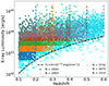Fig. 1.

Volume-limited selection of the eRASS1 cluster sample for our clustering study as a function of X-ray luminosity and redshift. The full sample is shown in cyan; the five subsamples are denoted in blue, orange, green, red, and pink.

Table 1.

Properties of the volume-limited eRASS1 cluster samples for our clustering study.

Motivated by the high purity of the catalogue thanks to P_cont, we additionally focused on a flux-limited sample up to z < 0.6 to infer cosmological parameters. We applied a luminosity cut at 10^42.7 erg s⁻¹, the same as for the volume-limited S0 sample. This allows us to discard the faintest structures. This final sample consists of 6493 clusters, with an average redshift of z = 0.307. This is the subsample covering the largest volume of 15.16 Gpc³ and is well suited for cosmological studies of the LSS of the Universe.

2.2. Random catalogue

The computation of the two-point correlation function (see Sect. 3) requires the generation of random points uniformly distributed on the sky, following the same geometrical properties and the redshift distribution of the eRASS:1 cluster catalogue. We started from the random catalogues provided by the Legacy Survey DR10³. They have a spatial density of 50 000 deg⁻². Following the optical selection of the eRASS1 primary sample (Bulbul et al. 2024; Kluge et al. 2024), we require coverage in the g, r, and z bands. We account for the cluster selection due to the varying eRASS1 exposure using the selection function from Clerc et al. (2024). It depends on count rate, redshift, exposure time, background and absorption. We randomly assigned count rates and redshifts to the random points by drawing samples from a Gaussian kernel distribution⁴ (Virtanen et al. 2020), generated from the eRASS1 digital twin from Seppi et al. (2022). The simulation is based on the cluster model from Comparat et al. (2020). We compute the probability of detection for each random point after fixing the exposure and background values from the eRASS:1 maps, and the nH values from HI4PI Collaboration (2016) at the position of each point. If the detection probability extracted from the selection function is larger than a random number between 0 and 1, we keep the random point in the catalogue.

This method provides a random catalogue that closely follows the angular and redshift distribution of the eRASS1 clusters by construction. The incompleteness of the eRASS1 sample, encoded in the selection function itself, is also naturally accounted for by our strategy. We show the spatial distribution on the sky in Fig. 2. The top panel shows the eRASS1 clusters, and the bottom one the random points. They are colour-coded according to their local density, estimated by a local kernel density estimation with scipy. After the selection function cut, the random catalogues are about 50 times larger than the eRASS1 samples.

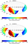Fig. 2.

Angular distribution of the selected eRASS:1 clusters (top panel) and the random points (bottom panel), after the application of the masks. The points are colour-coded according to their normalised local density. The density of the random catalogue changes through the sky very similarly to the eRASS1 data.

The number density as a function of redshift of the eRASS1 clusters and the random points is shown in Fig. 3. The histograms for the random populations are normalised to match the highest point of the cluster ones. The panel shows the two samples, respectively in blue and orange. The shape of the randoms redshift distribution captures the trend in the real data. We notice how the redshift distribution of the real eRASS1 is more peaked around z = 0.8, due to an optical filter transition. Although this is not a problem for the main cluster count analysis (Ghirardini et al. 2024) because of the redshift uncertainty evaluation, we restrict our analysis in the 0.1 < z < 0.6 range, where the redshift distributions of the random is similar to the data. We tested the reliability of our randoms by measuring the angular clustering of the eRASS1 clusters as a function of angular separation θ. We obtained a correlation function scaling with θ^−0.82, in agreement with the expected power law scaling with a slope of −0.8 (see e.g. Baugh & Efstathiou 1993; Maller et al. 2005).

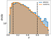Fig. 3.

Probability density redshift distribution of the selected eRASS:1 clusters and the random points. The panel shows the total number of clusters (randoms) in each redshift bin divided by the size of the bin in blue (orange), normalised by the integral over the redshift range. Two black vertical lines denote the redshift range used in our analysis, between 0.1 and 0.6. The bump in redshift at about 0.8 is due to a filter transition in the measurement of photo-z (see Kluge et al. 2024).

We also tried a more traditional method following the sensitivity maps (Georgakakis et al. 2008), used to construct random catalogues of point sources (Comparat et al. 2023). Although such a method is excellent for point sources, it is not ideal for extended ones. Within eSASS, the ersensmap task computing sensitivity maps for extended sources assumes a simple β-profile. Different works showed that the cluster detection is more complex (Clerc et al. 2018; Seppi et al. 2022). The random catalogue generated with this method may therefore introduce spurious clustering in the measurement of the correlation function. They are not used here.

3. Method

We measured the redshift-space two-point auto-correlation function for eRASS1 clusters on a two-dimensional grid of separation perpendicular and parallel to the line sight, respectively denoted as r_p and π (Fisher et al. 1994).

This strategy allows separating spatial correlations from redshift-space distortions due to large-scale bulk motions and intrinsic velocities (RSD, Kaiser 1987). We use the Landy-Szalay estimator (Landy & Szalay 1993):

$\begin{matrix} ξ (r_{p}, π) = 1 + \frac{N_{RR}}{N_{DD}} \frac{DD (r_{p}, π)}{RR (r_{p}, π)} - 2 \frac{N_{RR}}{N_{DR}} \frac{DR (r_{p}, π)}{RR (r_{p}, π)}, \end{matrix}$ $\begin{aligned} \xi (r_{\rm p},\pi ) = 1 + \frac{N_{\rm RR}}{N_{\rm DD}}\frac{\mathrm{DD}(r_{\rm p},\pi )}{\mathrm{RR}(r_{\rm p},\pi )} - 2 \frac{N_{\rm RR}}{N_{\rm DR}}\frac{\mathrm{DR}(r_{\rm p},\pi )}{\mathrm{RR}(r_{\rm p},\pi )}, \end{aligned}$ (1)

where DD(r_p, π), RR(r_p, π), and DR(r_p, π) are the number of pairs in two-dimensional bins of r_p and π for data, randoms, and data-random. The total pairs of data, randoms, and data-randoms are respectively denoted by N_DD = N_D(N_D − 1)/2, N_RR = N_R(N_R − 1)/2, and N_DR = N_DN_R. This estimator minimises variance and finite volume effects (Hamilton 1993).

We minimised the impact of RSD by computing the correlation function projected along the line of sight:

$\begin{matrix} w_{p} (r_{p}) = 2 \int_{0}^{π_{\max}} ξ (r_{p}, π) d π . \end{matrix}$ $\begin{aligned} { w}_{\rm p}(r_{\rm p}) = 2\int _0^{\pi _{\rm max}} \xi (r_{\rm p},\pi )\mathrm{d}\pi . \end{aligned}$ (2)

For our study, we consider ten logarithmic bins of separation r_p between 1 and 80 Mpc h⁻¹. We choose 1 Mpc h⁻¹ bins for π. In principle, π_max should extend to infinity. In practice, we use π_max = 100 Mpc h⁻¹ in this study. We tested other values of π_max equal to 80 and 120 Mpc h⁻¹ and found that they do not increase the signal-to-noise ratio compared to the chosen limit of 100 Mpc h⁻¹. For our purpose, this limit ensures the inclusion of correlated pairs and minimises the noisy contribution of distant ones. It allows the inclusion of pairs whose separation is well within the typical uncertainty on the photometric redshift with a mean scatter of 0.005 × (1 + z) (about 25 comoving Mpc at z = 0.3), see Kluge et al. (2024). We compute pair counts and the correlation function in Eqs. (1) and (2) with the software Corrfunc⁵ (Sinha & Garrison 2019, 2020).

We estimate the diagonal terms of the covariance matrix between different bins of separation with a jackknife method on the eRASS1 data. We created multiple subsamples of the cluster and random catalogues by removing different areas of about 54 deg² each time. Every area corresponds to a single HEALPix tile with NSIDE = 8⁶. Such a pixelisation divides the full sky into 768 pixels. We remove one area, compute a correlation function $w_{p}^{k}$ ${\it w}_{p}^k$ and iterate the process. Given the area covered by eRASS1, the removal of one pixel reduces the area by about 0.43%. We compute the jackknife covariance matrix according to

$\begin{matrix} {\hat{C}}_{i, j} = \frac{N_{S} - 1}{N_{S}} \sum_{k = 1}^{N_{S}} (w_{p, i}^{k} - \bar{w_{p, i}}) (w_{p, j}^{k} - \bar{w_{p, j}}), \end{matrix}$ $\begin{aligned} {\hat{\mathbf{C }}}_{i,j} = \frac{N_{\rm S}-1}{N_{\rm S}} \sum _{k = 1}^{N_{\rm S}} ({ w}_{p,i}^k - \overline{{ w}_{p,i}})({ w}_{p,j}^k - \overline{{ w}_{p,j}}), \end{aligned}$ (3)

where $w_{p, j}^{k}$ ${\it w}_{p,j}^k$ is the value of the k correlation function at separation j, $\bar{w_{p, i}}$ $\overline{\mathit{w}_{p,i}}$ is the average value of the correlation function at separation i, and N_S is the number of subsamples (Norberg et al. 2009).

To estimate the crossed terms of the covariance matrix we generate 1000 simulations using the Generator for Large-Scale Structure (GLASS, Tessore et al. 2023), creating shells with a depth of 200 comoving Mpc with a source density of 1 deg⁻². With this setup, we can study the correlation between separations with a source sky density that is similar to the average for eRASS1. We measure the correlation function for each realisation, compute a covariance matrix according to Eq. (3), and derive the correlation matrix c_{GLASS i, j}. Because these simulations do not include the selection function and the geometry of the survey, we only use them to estimate the relative correlation between crossed terms of the covariance matrix. We rely on the jackknife method for the diagonal terms. We combine them to generate the final covariance matrix:

$\begin{matrix} C_{i, j} = c_{GLASS i, j} \times [{\hat{C}}_{i, i} \otimes {\hat{C}}_{j, j}] . \end{matrix}$ $\begin{aligned} C_{i,j} = c_{\mathrm{GLASS}\,i,j} \times \left[{\hat{C}}_{i,i} \otimes {\hat{C}}_{j,j}\right]. \end{aligned}$ (4)

The correlation matrix C_i, j/ $\sqrt{C_{i, i} C_{j, j}}$ $\sqrt{C_{i,i}C_{j,j}}$ is shown in Fig. 4. The panel shows the correlation matrix c_{GLASS i, j}. The latter is rescaled by the diagonal terms for each sample according to Eq. (4). The figure highlights the low correlation between small and large scales, due to the separation between the 1-halo and 2-halo terms, around 2 Mpc h⁻¹. We further test and make sure that our method of estimating the off-diagonal terms of the covariance matrix with independent simulations does not bias our results in Appendix B.1.

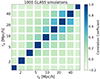Fig. 4.

Jackknife correlation matrix C_i, j/ $\sqrt{C_{i, i} C_{j, j}}$ $\sqrt{C_{i,i}C_{j,j}}$ for the projected correlation function of the eRASS1 cluster sample described in Sect. 2. The covariance matrix for the different samples presented in Sect. 2.1 is computed via jackknife (see Eq. (4)).

Given the excellent quality of the photometric redshifts, we do not account for additional redshift uncertainties (see Kluge et al. 2024). We further test this with the eRASS1 mock from Seppi et al. (2022). We measure the correlation function using the spectroscopic redshifts in the simulation. Then, we degrade them to mock photometric redshifts, adding a scatter σ_z(1 + z) around each spec-z, with σ_z equal to 0.5%, 1%, and 2%. We recompute the correlation functions with the mock photo-z and compare the result to the spec-z one. We repeat the process 100 times and analyze the median result. We provide more details in Appendix B.2. We obtain an impact of 1.7%, 2.3%, and 10.5% respectively for σ_z = 0.5%, σ_z = 1%, and σ_z = 2%. The uncertainty estimated from the diagonal elements of the covariance matrix gives a relative median 15.3% error. The 1-σ distribution around the median measurements is always compatible to the spec-z case for the σ_z = 0.5% test. We conclude that the photo-z uncertainty has a negligible impact on the measurement of the correlation function for our study. Future eROSITA data will allow us to increase the precision of the measurement, increasing the importance of the redshift estimate in the total error budget.

3.1. Models

The correlation function is the configuration space analogous to the matter power spectrum:

$\begin{matrix} ξ (r, z) = \frac{1}{2 π^{2}} \int d k k^{2} P_{M} (k, z = 0) D^{2} (z) \frac{sin (k r)}{kr}, \end{matrix}$ $\begin{aligned} \xi (r,z) = \frac{1}{2\pi ^2} \int \mathrm{d}k k^2 P_{\rm M}(k,z=0)D^2(z)\frac{\sin (kr)}{kr}, \end{aligned}$ (5)

where P_M(k, z) is the matter power spectrum and D²(z) is the growth factor normalised to 1 at z = 0. We denote physical distances with r, and redshift-inferred distances as s.

For the modelling, we convert π and r_p to the redshift-space radial distance and the angle between the line of sight and the direction of each pair according to:

$\begin{matrix} s = \sqrt{π^{2} + r_{p}^{2}} \\ μ = \frac{π}{s} \cdot \end{matrix}$ $\begin{aligned}&s = \sqrt{\pi ^2 + r_{\rm p}^2} \nonumber \\&\mu = \frac{\pi }{s}\cdot \end{aligned}$ (6)

We model the correlation function in redshift space according to

$\begin{matrix} ξ (s, μ) & = ξ_{0} (s) P_{0} (μ) + ξ_{2} (s) P_{2} (μ) + ξ_{4} (s) P_{4} (μ) \\ ξ_{0} (s) & = [1 + \frac{2}{3} β + \frac{1}{5} β^{2}] ξ (r) \\ ξ_{2} (s) & = [\frac{4}{3} β + \frac{4}{7} β^{2}] (ξ (r) - \bar{ξ} (r)) \\ ξ_{4} (s) & = \frac{8}{35} β^{2} [ξ (r) + \frac{5}{2} \bar{ξ} (r) - \frac{7}{2} \bar{\bar{ξ}} (r)], \end{matrix}$ $\begin{aligned} \xi (s,\mu )&= \xi _0(s)P_0(\mu ) + \xi _2(s)P_2(\mu ) + \xi _4(s)P_4(\mu ) \nonumber \\ \xi _0(s)&= \left[1+\frac{2}{3}\beta + \frac{1}{5}\beta ^2\right]\xi (r) \nonumber \\ \xi _2(s)&= \left[\frac{4}{3}\beta + \frac{4}{7}\beta ^2\right](\xi (r) - \overline{\xi }(r)) \nonumber \\ \xi _4(s)&= \frac{8}{35}\beta ^2 \left[\xi (r) + \frac{5}{2}\overline{\xi }(r) - \frac{7}{2}\overline{\overline{\xi }}(r)\right], \end{aligned}$ (7)

where ξ already accounts for the large-scale halo bias as explained in Sect. 3.1.1, P_ℓ are Legendre polynomials, ξ₀, ξ₂, ξ₄ are the monopole, dipole, and quadrupole moments of the 3D correlation function, $\bar{ξ} (r)$ $\overline{\xi}(r)$ and $\bar{\bar{ξ}} (r)$ $\overline{\overline{\xi}}(r)$ are integrals of the real space correlation function (see Hamilton 1992), and β = f/b is the ratio between the cosmic growth rate and the bias (Hamilton 1992; Valageas & Clerc 2012; Jeong et al. 2015). The growth rate is defined as the derivative of the growth factor D with respect to the scale factor a: f = dlnD/dlna (Peacock et al. 2001). We finally integrate the model in Eq. (7) according to Eq. (2) to obtain a prediction of the two-point correlation function projected along the line of sight.

3.1.1. HOD

We interpret the eRASS1 correlation function using the Halo Occupation Distribution formalism (Kravtsov et al. 2004; Zheng et al. 2005). Following the example of More et al. (2015), we parametrise the HOD models as

$\begin{matrix} N_{C} (M | M_{\min}, σ_{log M}) = f_{inc} (M) \frac{1}{2} [1 + \erf (\frac{log (M / 10^{M_{\min}})}{σ_{log M}})] \\ N_{S} (M | M_{sat}, α_{sat}) = N_{C} {(\frac{M - 10^{M_{sat} - 1}}{10^{M_{sat}}})}^{α_{sat}} \\ f_{inc} (M | α_{inc}, M_{inc}) = max [0, min [1, 1 + α_{inc} (log M - log M_{inc})]] . \end{matrix}$ $\begin{aligned}&N_{\rm C}(M | M_{\rm min}, \sigma _{\log \mathrm{M}}) = f_{\rm inc}(M) \frac{1}{2} \left[1+\mathrm{erf} \left(\frac{\log (M/10^{M_{\rm min}})}{\sigma _{\log \mathrm{M}}}\right)\right]\nonumber \\&N_{\rm S}(M | M_{\rm sat}, \alpha _{\rm sat}) = N_{\rm C} \left(\frac{M - 10^{M_{\rm sat}-1}}{10^{M_{\rm sat}}}\right)^{\alpha _{\rm sat}}\nonumber \\&f_{\rm inc}(M | \alpha _{\rm inc}, M_{\rm inc}) = {\max }[0, {\min }[1, 1+\alpha _{\rm inc}(\log M - \log M_{\rm inc})]]. \end{aligned}$ (8)

Our model depends on four free parameters: M_min is the typical mass of a dark matter halo that starts being populated by sources in our sample, σ_logM describes the sharpness of the transition between unpopulated and populated dark matter haloes, M_sat and α_sat define the power law describing the average number of satellites (i.e. low-mass haloes companion to massive clusters). We also account for the incompleteness in the eRASS1 cluster samples, based on the eRASS1 digital twin (Seppi et al. 2022) and fit it with the incompleteness function in Eq. (8) using the curve_fit package⁷. We do not find a significant dependence on the slope α_inc for different samples. Therefore, we fix it to 0.55. We report the best-fit values in Table 2. We find a progressively lower M_inc parameter, decreasing from 15.25 for the S4 sample to 14.87 for the S0 one. It means that deeper samples start being incomplete at lower masses.

Table 2.

Priors and posteriors for the HOD and the derived parameters on the five volume-limited eRASS1 samples (see Table 1 and Fig. 1).

Finally, we infer the fraction of satellites by weighting the number of satellites by the halo mass function compared to the sum of satellites and centrals:

$\begin{matrix} f_{sat} = \frac{\int \int N_{S} (M) \frac{d n}{d M} d V d M}{\int \int N_{TOT} (M) \frac{d n}{d M} d V d M}, \end{matrix}$ $\begin{aligned} f_{\rm sat} = \frac{\int \int N_{\rm S}(M)\dfrac{\mathrm{d}n}{\mathrm{d}M}\mathrm{d}V\mathrm{d}M}{\int \int N_{\rm TOT}(M)\dfrac{\mathrm{d}n}{\mathrm{d}M}\mathrm{d}V\mathrm{d}M}, \end{aligned}$ (9)

where N_TOT = N_C + N_S and dn/dM(M) is the dark matter halo mass function. We use the halo mass function model from Tinker et al. (2008). We tested other halo mass functions from Despali et al. (2016) and Seppi et al. (2021). We verified that the chosen mass function model does not significantly affect our results.

We model the power spectrum according to Asgari et al. (2023). The power spectrum prediction includes multiple terms as follows:

$\begin{matrix} P (k, z) = & 2 P_{c, s}^{1 h} (k, z) + P_{s, s}^{1 h} (k, z) + P_{c, s}^{1 h} (k, z) \\ + P_{c, c}^{2 h} (k, z) + 2 P_{c, s}^{2 h} (k, z) + P_{s, s}^{2 h} (k, z) . \end{matrix}$ $\begin{aligned} P(k,z) =&2P_{\rm c,s}^\mathrm{1h}(k,z) + P_{\rm s,s}^\mathrm{1h}(k,z) + P_{\rm c,s}^\mathrm{1h}(k,z)\nonumber \\&+P_{\rm c,c}^\mathrm{2h}(k,z) + 2P_{\rm c,s}^\mathrm{2h}(k,z) + P_{\rm s,s}^\mathrm{2h}(k,z). \end{aligned}$ (10)

The subscripts c and s refer to central and satellite objects. The overscripts 1h and 2h indicate 1-halo and 2-halo terms. The correlation between central objects in two separate haloes is then $P_{c, c}^{2 h}$ $P_{\mathrm{c,c}}^{\mathrm{2h}}$ , the one between satellites in the same halo is $P_{s, s}^{1 h}$ $P_{\mathrm{s,s}}^{\mathrm{1h}}$ . Each term is a mass integral including the quantities in Eq. (8). The large-scale halo bias is finally inferred by convolving the Tinker et al. (2010) model with central, satellites, and the halo mass function in a mass integral (Berlind & Weinberg 2002), providing more flexibility compared to a strict choice of bias model thanks to the self-consistent HOD modelling. The power spectrum in Eq. (10) is used to derive the correlation function ξ in Eq. (7). We refer the reader to More et al. (2015) for more details on the formalism for each term of Eq. (10) and to van den Bosch et al. (2013) for the general theoretical framework.

We predict HOD models of the correlation functions with AUM⁸ (van den Bosch et al. 2013; More 2021). This software uses the M_200b mass definition, corresponding to the mass enclosed by a radius encompassing an average density equal to 200 times the background matter density. Therefore, we quote HOD results in terms of M_200b in the rest of the article, if not otherwise stated.

3.1.2. Cosmology

For the cosmological study, we focus on a flux-limited sample of 6493 clusters, spanning the redshift range 0.1−0.6, with X-ray luminosity larger than 5 × 10⁴² erg s⁻¹ (a cut in log at 42.7). This sample covers the largest cosmological volume of 15.16 Gpc³. The sample selection is explained in Sect. 2.1.

A key ingredient of a clustering analysis is the prescription for the large-scale halo bias model. A common strategy consists of using a scaling relation approach to obtain halo masses from observables such as X-ray luminosity or richness (Lindholm et al. 2021; Lesci et al. 2022b). More recently, the development of emulators allows a fast prediction of clustering measurements that intrinsically include the bias (Nishimichi et al. 2019; Sunayama et al. 2023). Although a theoretical estimate of the bias in the cluster regime is possible (Sheth & Tormen 1999), one limitation is the precision and accuracy of different halo bias models. Clusters of galaxies are strongly biased tracers of the LSS, and various models show discrepancies even > 20% in this regime (Tinker et al. 2010; Bhattacharya et al. 2011; Comparat et al. 2017; Lindholm et al. 2021). The choice of a specific model at fixed mass may bias cosmological results. Therefore, we take advantage of our HOD approach to model the bias in a self-consistent way, with no prior assumption on halo mass as explained in Sect. 3.1.1. We develop a cosmological fitting method that models the large-scale halo bias together with halo occupation in a flexible manner. We use σ_logM, α_sat, and M_sat as nuisance parameters, sampling a uniform prior containing the best-fit HOD results of each volume-limited sample in Table 1. With this method, we are not affected by fixed parameters obtained from the HOD fits in a fixed cosmology. We sample M_min together with cosmological parameters to account for the cosmological dependency of the halo bias on the clustering amplitude.

We predict models of the correlation function with the AUM software described in the previous section. It predicts power spectra based on Eisenstein & Hu (1998) for the linear power spectrum and the transfer function T²(k, z), and Smith et al. (2003) for the non-linear regime. We use the same binning scheme as for the HOD modelling. The impact of non-linearities (Angulo et al. 2021; Angulo & Hahn 2022) is intrinsically included in the HOD approach. Extending this study to even larger scales ≳100 Mpc h⁻¹ requires additional modelling of the baryonic acoustic oscillations (BAO) peak (Veropalumbo et al. 2016). The moments of ξ(s) in Eq. (7) are computed by convolving the non-linear matter power spectrum with Bessel functions using FFTLog (Hamilton 2000) within GSL⁹.

We account for the Alcock & Paczynski (1979, AP) geometrical distortions of the correlation function via the α_∥ and α_⊥ parameters, defined according to

$\begin{matrix} π & = α_{‖} π^{fid} \\ r_{p} & = α_{⊥} r_{p}^{fid} \\ α_{‖} & = \frac{H^{fid} (z)}{H (z)} \\ α_{⊥} & = \frac{D_{A} (z)}{D_{A}^{fid} (z)}, \end{matrix}$ $\begin{aligned} \pi&= \alpha _\parallel \pi ^\mathrm{fid} \nonumber \\ r_{\rm p}&= \alpha _\perp r_{\rm p}^\mathrm{fid} \nonumber \\ \alpha _\parallel&= \frac{H^\mathrm{fid}(z)}{H(z)} \nonumber \\ \alpha _\perp&= \frac{D_{\rm A}(z)}{D_{\rm A}^\mathrm{fid}(z)}, \end{aligned}$ (11)

where H(z) is the Hubble parameter, D_A(z) is the angular diameter distance, and the overscript “fid” denotes the quantity computed by assuming a fiducial cosmology (the one from Planck Collaboration VI 2020, in this study) to convert redshifts to distances. The model of the correlation function is then evaluated at separation equal to $α_{⊥} r_{p}^{fid}$ $\alpha_\perp r_{\mathrm{p}}^{\mathrm{fid}}$ (α_∥π^fid) in the direction perpendicular (parallel) to the line of sight.

We follow the evolution mapping approach from Sánchez (2020), Sánchez et al. (2022) to infer cosmological parameters in an h-independent way. We consider physical densities $ω_{i} = \frac{8 π G}{3 H_{100}^{2}} ρ_{i}$ $\omega_i=\dfrac{8\pi G}{3H^2_{100}}\rho_i$ , where ρ_i is the density of each component at the present day, and H₁₀₀ = 100 km s⁻¹ Mpc⁻¹. We fix the value of the scalar spectral index and the baryons density according to the results of Planck Collaboration VI (2020) to n_s = 0.9665 and ω_b = 0.02242. Given that clustering studies with galaxy clusters strongly depend on the matter density, we let the physical cold dark matter density ω_c free to vary. We free parameters affecting the evolution of the power spectrum, such as its normalisation A_s, and the physical dark energy density ω_DE. We fix the dark energy equation of state to w₀ = −1 and w_a = 0, and assume a flat Universe Ω_K = 0. With this approach, the Hubble parameter is recovered by construction as $h = \sqrt{ω_{c} + ω_{b} + ω_{DE}}$ $h=\sqrt{\omega_{\mathrm{c}} + \omega_{\mathrm{b}} + \omega_{\mathrm{DE}}}$ .

3.2. Likelihood

Given the HOD parametrisation, we require our best fit to maximise a Gaussian likelihood. We compute it according to

$\begin{matrix} log L = - \frac{1}{2} {[D - M (θ)]}^{T} C_{ij}^{- 1} [D - M (θ)], \end{matrix}$ $\begin{aligned} \log \mathcal{L} = - \frac{1}{2}[\mathbf D -\mathbf M (\theta )]^T \mathbf{C }_{ij}^{-1}[\mathbf D -\mathbf M (\theta )], \end{aligned}$ (12)

where D is the data array for each projected correlation function, M is the w_p(r_p) model that depends on the array of parameters θ. We fit five HOD models independently for each volume-limited sample in Table 1. Each sample has a different covariance matrix, as explained in Sect. 3. We use the same likelihood form to fit cosmological parameters together with the HOD ones (see Sect. 3.1.2).

We derive posterior probability distributions and the Bayesian evidence with the nested sampling Monte Carlo algorithm MLFriends (Buchner 2016, 2019) using the UltraNest¹⁰ package (Buchner 2021). We quote as best-fit parameters the 50% quantile of the marginalised posterior distributions. The uncertainty on the parameters includes the 16th–84th percentile. The upper limits extend to the 84th percentile.

4. Results

We present our results in this section. The HOD interpretation is described in Sect. 4.1. The cosmological implications are reported in Sect. 4.3.

4.1. HOD interpretation

We show the correlation functions and the best-fit models in Fig. 5. For clarity, we shift the correlation functions by factors equal to e⁰ for S0, e¹ for S1, e² for S2, e³ for S3, e⁴ for S4. The models in Eq. (8), shown by the solid lines, represent the measurement well. The shaded areas show the 1- and 2-σ uncertainties on the models. The total signal-to-noise ratio of the correlation function for each sample is 29.9, 39.4, 41.1, 35.4, and 29.7 from S0 to S4. The S4 sample (in violet) has the highest clustering signal, in agreement with the fact that it contains the largest fraction of the most massive objects. On the other hand, the S0 sample (in blue) probes lower mass clusters and groups and the clustering signal is lower, in agreement with expectations.

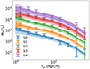Fig. 5.

Projected correlation functions of the volume selected eRASS1 clusters samples. Each colour denotes one sample. The error bars show the measurement, the solid line is the best fit model, and the shaded areas denote the 1-σ and 2-σ uncertainty on the model. For clarity, we shift the measurements and models by e^{0, 1, 2, 3, 4} from S0 to S4.

The best-fit parameters are reported with the respective priors in Table 2. The M_min parameter decreases from 15.04 $_{- 0.72}^{+ 0.61}$ $^{+0.61}_{-0.72}$ to 14.73 $_{- 0.35}^{+ 0.93}$ $^{+0.93}_{-0.35}$ from the S4 to the S0 sample. It is in agreement with eROSITA probing the lower mass cluster population at low redshift. The σ_logM parameter decreases with redshift increasing. The S4 sample prefers a quick transition for the population of dark matter haloes to host X-rays seen by eROSITA as a function of mass. For the S0 sample, the introduction of lower mass clusters and groups makes the transition smoother. The result is a larger σ_logM, increasing from 0.57 $_{- 0.37}^{+ 0.20}$ $^{+0.20}_{-0.37}$ to 0.82 $_{- 0.46}^{+ 0.49}$ $^{+0.49}_{-0.46}$ from S4 to S0. The transition is nonetheless much sharper compared to AGN in the eROSITA Final Equatorial Depth Survey (eFEDS), where Comparat et al. (2023) measured σ_{log M} = 1.26. Similarly, the slope of the power law describing the satellites α_sat is shallower for the low-mass samples, varying from 1.25 $_{- 0.54}^{+ 0.89}$ $^{+0.89}_{-0.54}$ to 1.67 $_{- 1.08}^{+ 1.05}$ $^{+1.05}_{-1.08}$ from S0 to S4. For clusters and groups, the slope is steeper compared to eFEDS AGN (α_sat = 0.73, Comparat et al. 2023), showing that according to our model the satellite population becomes quickly subsidiary as mass decreases in our study. The M_sat parameter assumes high values, that increase from 15.32 $_{- 0.33}^{+ 0.34}$ $^{+0.34}_{-0.33}$ for S0 to 15.76 $_{- 0.55}^{+ 0.42}$ $^{+0.42}_{-0.55}$ for S4. If satellite objects are rare, the HOD model will push the M_sat parameter to high values, fitting the correlation function mostly with signal from the central objects. We notice that most of the HOD parameters for different samples are compatible within uncertainties. Nonetheless, we see a trend for the median values from the faint low-z population to the bright high-z one in our volume-limited selection. Deeper data in future eRASS surveys with larger samples will reduce the uncertainty on the measure of the correlation functions due to the lower Poisson noise and help shed light on the satellite population of massive dark matter haloes in the clusters and groups regime.

We estimate the posterior distribution after accounting for the prior boundaries with the GetDist¹¹ software (Lewis 2019). The full marginalised posterior distributions are shown in Fig. 6. The five samples (S0, S1, S2, S3, S4) are shown in different colours (blue, orange, green, red, violet). The positive degeneracy between M_min and σ_logM is expected because a similar population of centrals may be described by a high cutoff mass but a broader transition or vice versa. The same holds for the negative degeneracy between M_sat and α_sat, with a steep power law anchored at large satellite masses explaining the same population of a shallower satellite function starting from lower masses. Together with σ_logM, α_sat is the HOD parameter with the broadest posterior. Because the shape of the posterior distribution is complex, it may depend on the choice of the prior. We tested larger and smaller prior distributions compared to the ones reported in Table 2 for the S2 sample. We obtained compatible results for each case, with excellent agreement between the choice made for this analysis and larger distributions. We conclude that the choice of the prior does not strongly affect our results. We provide more details on this test in Appendix B.3.

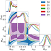Fig. 6.

Marginalised posterior distributions of the best fit HOD parameters. The filled 2D contours show the 1-σ and 2-σ confidence levels of the posteriors after convolution with the uniform priors. The model is given by Eq. (8). The corresponding 1D parameter constraints are reported in Table 2.

We obtain the occupation distribution of central and satellite X-ray haloes seen by eROSITA as a function of mass for each volume-limited selected sample. The result is shown in Fig. 7. The average number of centrals (satellites) in a halo of mass M is shown by the dotted (dashed) lines. According to our models, haloes more massive than 3.0 (6.5)×10¹⁵ M_⊙ start hosting more than one satellite on average for the S0 (S4) sample. We obtain upper limits for the satellite fraction, which varies from < 14.9% to < 8.1% from S0 to S4. Our result confirms the general assumption that clusters detected in eRASS1 populate distinct haloes and the traditional halo mass function formalism for cluster abundance holds (Ghirardini et al. 2024).

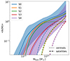Fig. 7.

Derived distribution of the eRASS1 clusters and groups population in dark matter haloes (solid lines), divided in central (dashed) and satellite (dotted) objects. The colours denote each volume-limited sample (see Table 1). The shaded areas denote the 1-σ confidence levels on the model. For clarity, only the S0 and S4 samples are shown.

We find an increasing average halo bias as a function of mass and redshift. This is in agreement with a bottom-up structure formation scenario. The bias changes by 47% from b = 2.95 ± 0.21 in the S0 sample to b = 4.34 ± 0.62 in S4. The bias as a function of the X-ray luminosity from Bulbul et al. (2024) for each sample is shown in Fig. 8. The panel is colour-coded by the average redshift of each sample. We fit a linear relation between the bias and log L_X with curve_fit in the form b = m(log L_X − 44)+q. We find a slope of m = 2.58 ± 0.11 and a zero point of q = 3.32 ± 0.02. The slope is much steeper in the cluster regime compared to AGN. In the clustering study of eFEDS, Comparat et al. (2023) combine their results with Krumpe et al. (2015) and find a slope of 0.492. This is expected due to the strong dependency of the bias on halo mass. We compare our results to other bias models at the average redshift and inferred mass for the S0 and S4 samples. Our results are compatible with the bias models from Sheth et al. (2001) respectively equal to 3.10 and 4.27, Tinker et al. (2010) equal to 3.14 and 4.56, Comparat et al. (2017) equal to 3.12 and 4.46. The models from Sheth & Tormen (1999) (2.81 and 3.88) and Bhattacharya et al. (2011) (2.68 and 3.83) underpredict our result. In Fig. 9 we show a comparison with bias values from other surveys and probes. For the DES-Y1 redmapper clusters (Rykoff et al. 2016) we derived an average halo bias with the model from Tinker et al. (2010) using halo masses from the weak lensing richness-mass scaling relation from McClintock et al. (2019). Together with other cluster samples, our eRASS1 results show large bias values b > 3, compared to galaxies and AGN with values that are typically lower.

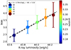Fig. 8.

Large-scale halo bias as a function of average X-ray luminosity for the eRASS1 volume-limited samples. Each point is colour-coded by the average redshift of the sample. The black line shows the best-fit linear relation.

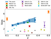Fig. 9.

Comparison between the halo bias of eRASS1 clusters (in blue) with other experiments and probes from Planck clusters in orange (Lesci et al. 2023), CODEX clusters in green (Lindholm et al. 2021), XXL clusters in red (Marulli et al. 2018), DES-Y1 clusters in purple (Rykoff et al. 2016), eFEDS AGN in brown (Comparat et al. 2023), RASS AGN in pink (Krumpe et al. 2015), DES-Y1 galaxies in grey (Elvin-Poole et al. 2018), DES-Y3 galaxies in yellow (Abbott et al. 2022), and SDSS-DR7 galaxies selected in stellar mass in cyan (Zu & Mandelbaum 2015).

We infer the average halo mass for each volume-limited cluster sample from the best-fit HOD. We confirm that the low-luminosity samples probe less massive haloes by inferring the halo mass populated by the five volume-limited samples from the HOD models. We find an average mass of 3.09 ± 0.48 × 10¹⁴ M_⊙ for S0, compared to 4.38 ± 1.11 × 10¹⁴ M_⊙ for S4. We convert M_200b to M_500c using the relations from Ragagnin et al. (2021). In terms of M_500c we obtain 1.58 ± 0.25 × 10¹⁴ M_⊙ for S0 and 2.42 ± 0.61 × 10¹⁴ M_⊙ for S4. The median value of the primary sample is 1.8 × 10¹⁴ M_⊙ (Bulbul et al. 2024). Given the selection of our samples (see Table 1) we are well-aligned with the catalogue measurement. We then convert the average X-ray luminosity in the 0.2−2.3 keV band to 0.5−2.0 keV by computing conversion factors with Xspec (Arnaud 1996), assuming an apec model with the average temperature of the eRASS1 sample of kT = 2.04 keV (Bulbul et al. 2024). The L_X − M_500c scaling relation is shown in Fig. 10. Our data points are shown in blue. The green dots show a collection of clusters from Lovisari et al. (2015, 2020), Mantz et al. (2016), Schellenberger & Reiprich (2017), Adami et al. (2018), Bulbul et al. (2019), and eFEDS (Liu et al. 2022). The red dots highlight the eRASS1 sample (Bulbul et al. 2024). The black line denotes a simple linear fit on our data and does not account for the selection function. We find a slope of 1.87 ± 0.34 and a zero point of 16.9 ± 4.2. Our result is compatible within 1σ with previous results in the literature (Pratt et al. 2009; Lovisari et al. 2015; Bulbul et al. 2019; Capasso et al. 2020; Chiu et al. 2022). In addition, we combine constraints from N_C and w_p(r_p) to calibrate a HAM model using the eRASS1 clusters (see Sect. 4.2). We infer a scatter between X-ray luminosity and halo mass of σ_Lx = 0.36, shown by the shaded area in Fig. 10. Our HOD approach anchors the X-ray-mass scaling relation with a new method, independent from mass calibration techniques using weak lensing of dynamical mass measurements, the results agree with previous studies.

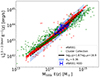Fig. 10.

Scaling relation between halo mass and X-ray luminosity. The halo mass is inferred from our best-fit HOD (in blue). The black line shows a linear fit to our data points. The green dots denote a collection of clusters from Lovisari et al. (2015, 2020), Mantz et al. (2016), Schellenberger & Reiprich (2017), Adami et al. (2018), Bulbul et al. (2019), and Liu et al. (2022). The eRASS1 sample is denoted in red (Bulbul et al. 2024). The shaded area includes a scatter σ_Lx = 0.36 around the mean relation, obtained by the halo abundance matching explained in Sect. 4.2. The extrapolated scaling relation outside the parameter space sensitive to our HOD approach is indicated with the dashed black line and the hatched shaded area.

We compare the excess surface density prediction from our best-fit HOD models to lensing data in Appendix A.

4.2. Halo abundance matching predictions

An alternative scheme to the HOD to model clustering measurements is halo abundance matching (e.g. Kravtsov et al. 2004; Guo et al. 2016). It consists in using numerical N-body simulations (in a fixed cosmology) and devising a subhalo selection procedure to match the observed number density of tracers as a function of redshift (Rodríguez-Torres et al. 2016, 2017; Favole et al. 2016; Guo et al. 2019).

To construct an abundance matching model of X-ray selected clusters, we use the HugeMultiDarkPlanck (HMD) simulation (Klypin et al. 2016), a dark matter only simulation with a 4 h⁻¹ Gpc box size. We add a scatter σ_HAM around halo masses with values spanning from σ_HAM = 0 to 1 and intervals of 0.01, exploring the parameter space with 100 σ_HAM values. We then sort the values of mass and keep the most massive systems in the HAM samples to match the number density of sources in each eRASS1 volume selected sample (see Table 1). We obtain a HAM prediction for N_C by normalising the mass histogram of each HAM sample with the mass histogram of the full HMD simulation. We also compute the projected correlation function for each HAM sample. Figure 11 shows the result for S0 on the left and S4 on the right. The shaded areas denote the measurement of the eRASS1 correlation function and the HOD result, the HAM predictions with different values of the scatter σ_HAM are shown by the coloured lines. We find an overall good agreement between the HOD and HAM predictions.

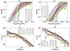Fig. 11.

Comparison between the HOD results from Sect. 4.1 and the abundance matching procedure. The top panels show the prediction for the number of central objects as a function of mass, the bottom panels show the projected correlation function. For clarity, only 9 of the 100 HAM predictions are shown. The panels on the left refer to the S0 sample and the ones on the right to the S4 one. The shaded areas denote the results and measurements from the data; the coloured lines show the HAM predictions with different values of the scatter σ_HAM.

To find the optimal value of σ_HAM, we compute two distances between the HAM prediction compared to best-fit HOD prediction for the number of centrals as a function of mass (d_Nc) and the projected correlation function (d_wp), according to:

$\begin{matrix} d_{Nc} (σ_{HAM}) & = \frac{1}{N_{M}} \sum_{M} \frac{{[N_{HAM} (M, σ_{HAM}) - N_{HOD}^{50 %} (M)]}^{2}}{{[N_{HOD}^{84 %} (M) - N_{HOD}^{16 %} (M)]}^{2}} \\ d_{Wp} (σ_{HAM}) & = \frac{1}{N_{rp}} \sum_{r_{p}} \frac{{[w_{p, HAM} (r_{p}, σ_{HAM}) - w_{p, HOD}^{50 %} (r_{p})]}^{2}}{{[w_{p, HOD}^{84 %} (r_{p}) - w_{p, HOD}^{16 %} (r_{p})]}^{2}}, \end{matrix}$ $\begin{aligned} d_{\rm Nc}(\sigma _{\rm HAM})&= \frac{1}{N_{\rm M}} \sum _{\rm M} \frac{[N_{\rm HAM}(M,\sigma _{\rm HAM}) - N_{\rm HOD}^\mathrm{50\%}(M)]^2}{[N_{\rm HOD}^{84\%}(M) - N_{\rm HOD}^\mathrm{16\%}(M)]^2}\nonumber \\ d_{\rm Wp}(\sigma _{\rm HAM})&= \frac{1}{N_{\rm rp}} \sum _{\rm r_{\rm p}} \frac{[{ w}_{\rm p,HAM}(r_{\rm p},\sigma _{\rm HAM}) - { w}_{\rm p,HOD}^\mathrm{50\%}(r_{\rm p})]^2}{[{ w}_{\rm p,HOD}^{84\%}(r_{\rm p}) - { w}_{\rm p,HOD}^\mathrm{16\%}(r_{\rm p})]^2}, \end{aligned}$ (13)

where N_M (N_rp) is the number of mass (projected separation) bins. We account for the uncertainty on the HOD model through the 16th and 84th percentiles of each distribution. Our formulation is very similar to the one adopted by Comparat et al. (2023) for the HOD prediction, here we also include the correlation function term. We evaluate the allowed σ_HAM space as follows. For each σ_HAM, we check whether both d_Nc(σ_HAM) and d_Nc(σ_HAM) are less than one (i.e. the difference between the best-fit HOD and the HAM prediction is within the HOD uncertainty). If this is the case, we mark the value of σ_HAM as allowed. We infer the optimal σ_HAM by averaging over the values allowed for each volume-limited sample. As Fig. 11 shows, the constraint from w_p(r_p) easily discards the highest values of σ_HAM, whereas the one from N_C helps excluding the lowest ones.

By construction, the HAM strictly depends on halo properties, in our case halo mass. Because of the X-ray luminosity cut in the eRASS1 volume-limited samples, our selection is not exactly mass-limited but includes the scatter of the observable (in this case L_X) around halo mass. The σ_HAM parameter naturally accounts for it and is therefore related to the scatter in the scaling relation between L_X and halo mass (Guo et al. 2016). In other words, a HAM with σ_HAM = 0 would reflect an observable capable of perfectly tracing halo mass. It is then possible to deduce the average X-ray luminosity scatter at fixed mass by accounting for the slope m = 1.87 of the L_X − M_500c scaling relation from Sect. 4.1 and assuming that such scatter is lognormal. The end result is $σ_{Lx} = \frac{m σ_{HAM}}{\sqrt{2}}$ $\sigma_{\mathrm{Lx}} = \dfrac{m\sigma_{\mathrm{HAM}}}{\sqrt{2}}$ (see Zheng et al. 2007; Guo et al. 2016). We collect the results in Table 3.

Table 3.

Optimal values of the scatter parameter σ_HAM for each volume-limited sample.

Albeit our constraints are broad and the σ_HAM are compatible within error bars with each other, we find that on average it decreases by about 60% from 0.44 for S0 to 0.17 for S4. This is in agreement with our HOD results and the sharper selection for luminous massive clusters. By averaging over the individual inferred luminosity-mass scatter on each sample, we find ⟨σ_Lx⟩ = 0.36 ± 0.12 for eRASS1. Therefore, we add such scatter to the scaling relation obtained in Sect. 4.1 (Fig. 10). Part of this is scatter resides in the intrinsic nature of clusters, for example, different core properties are reflected in varying luminosities at fixed halo mass. In addition, the luminosity selection from the eROSITA survey adds an additional component to the scatter. This description is consistent with our result in comparison to the X-ray cluster model from Comparat et al. (2020), who find an intrinsic scatter of 0.21. The model does not include the secondary scatter component due to the survey selection function. Finally, our result encompasses the cluster samples from different surveys with good agreement (see Fig. 10). In particular, Bulbul et al. (2019) found a scatter of $0 . 27_{- 0.12}^{+ 0.08}$ $0.27^{+0.08}_{-0.12}$ for an SZ-selected sample around the mean scaling relation, compatible with our result within 1σ.

In summary, the HAM procedure starts from a set of dark matter haloes generated by a Universe with Planck Collaboration XIII (2016) cosmology, the one assumed by the HMD simulation. The fact that the σ_HAM obtained with our method is in agreement with the literature means that this study with eRASS1 clusters does not exclude such set of cosmological parameters. From the HAM perspective, we conclude that our results are compatible with the Planck Collaboration XIII (2016) cosmology.

4.3. Cosmological implications

For the inference of cosmological parameters, we focus on a flux-limited sample of 6493 sources with the same luminosity cut of S0. We still consider the redshift range 0.1 < z < 0.6. The efficient removal of contaminants (see Sect. 2), makes it suitable also for cosmological studies. The methodology is explained in Sect. 3.1.2. Thanks to the larger number of clusters in this sample compared to the volume-limited ones, the signal-to-noise ratio is larger and reaches 50.1. Figure 12 shows the measured correlation function with error bars in blue and the best-fit cosmological model in red. The shaded areas denote the 1- and 2-σ uncertainty on the model.

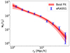Fig. 12.

Projected correlation functions of the eRASS1 clusters. The error bars show the measurement, the solid line is the best fit cosmological model, and the shaded areas denote the 1-σ and 2-σ uncertainty on the model.

We interpret our results in terms of the clustering amplitude σ₁₂ (Sánchez et al. 2022), encoding the variance of the density field smoothed on scales of 12 Mpc. It is defined according to

$\begin{matrix} σ_{12}^{2} = \frac{1}{2 π^{2}} \int d k k^{2} P_{lin} (z = 0, k) \tilde{W} (k \times 12 Mpc), \end{matrix}$ $\begin{aligned} \sigma _{12}^2 = \frac{1}{2\pi ^2}\int \mathrm{d}k k^2 P_{\rm lin}(z=0,k)\tilde{W}(k \times 12\,\mathrm{Mpc}), \end{aligned}$ (14)

where P_lin is the linear matter power spectrum, and $\tilde{W}$ $\tilde{W}$ is the Fourier transform of a top-hat filter with a radius of 12 Mpc. σ₁₂ has the advantage of depending on the Hubble parameter only through the amplitude of the power spectrum, not on the reference smoothing scale. This allows us to disentangle the dependency of the clustering amplitude on A_s through σ₁₂ from the one on the reference scale encoded in h.

The prior and the posteriors for the cosmological parameters are reported in Table 4. We obtain the large-scale halo bias as a derived parameter from the HOD formalism. We measure $ω_{c} = 0 . 12_{- 0.02}^{+ 0.03}$ $\omega_{\mathrm{c}}=0.12^{+0.03}_{-0.02}$ , $ln 10^{10} A_{s} = 2 . 92_{- 0.53}^{+ 0.55}$ $\ln 10^{10}A_{\mathrm{s}}=2.92^{+0.55}_{-0.53}$ , and $M_{\min} = 14 . 74_{- 0.24}^{+ 0.28}$ $M_{\mathrm{min}}=14.74^{+0.28}_{-0.24}$ . We infer the derived parameters $b = 3 . 63_{- 0.85}^{+ 1.02}$ $b=3.63^{+1.02}_{-0.85}$ , $σ_{12} = 0 . 77_{- 0.16}^{+ 0.22}$ $\sigma_{12}=0.77^{+0.22}_{-0.16}$ , $Ω_{M} = 0 . 32_{- 0.03}^{+ 0.04}$ $\Omega_{\mathrm{M}}=0.32_{-0.03}^{+0.04}$ , and $σ_{8} = 0 . 76_{- 0.16}^{+ 0.22}$ $\sigma_{8}=0.76^{+0.22}_{-0.16}$ . Our constraining power on ω_DE is weak, and the best-fit value we get from the posterior fills the prior. Therefore, the H₀ constraint is conservative. Our results are compatible within 1-σ with state-of-the-art results from the cosmic microwave background (CMB) analysis (Planck Collaboration VI 2020) and provide an independent test for the vanilla ΛCDM cosmological model.

Table 4.

Priors and posteriors on the cosmology and large-scale halo bias parameters.

The panels in Fig. 13 show the full marginalised posterior distribution. As expected, we find a strong negative degeneracy between the large-scale-halo bias and the clustering amplitude σ₁₂. The relative correlation coefficient is −0.91. They are both directly related to the overall normalisation of the correlation function. Because of this aspect, the constraining power on σ₁₂ (and similarly for σ₈) is weak, which also makes the ω_c − σ₁₂ 2D posterior distribution broad. We compare the h-independent cosmological parameters and the traditional ones in Fig. 14. The eRASS1 clustering constraints are shown in blue, and the CMB ones from Planck Collaboration VI (2020) in orange. We find a positive degeneracy between ω_c and ω_DE, with a correlation coefficient of 0.61. The same behaviour was obtained by Semenaite et al. (2022) in a clustering study of the Extended Baryon Oscillation Spectroscopic Survey (eBOSS). The same LSS at redshift about 0.3 can be generated in a Universe with a high physical matter density facilitating halo collapse and a large amount of dark energy contrasting the collapse, or vice versa. The difference between such scenarios resides in the expansion factor regulated by H₀. The correlation between Ω_M and H₀ is in fact negative, with a coefficient of −0.27.

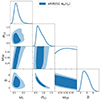Fig. 13.

Marginalised posterior distributions of the best-fit cosmological parameters. The 1-σ and 2-σ confidence levels of the posteriors are shown as filled 2D contours. The model is explained in Sect. 3.1.2. The parameters are reported in Table 4.

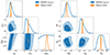Fig. 14.

Marginalised posterior distributions of the best-fit cosmological parameters. The 1-σ and 2-σ confidence levels of the posteriors are shown as filled 2D contours. The model is explained in Sect. 3.1.2. The parameters are reported in Table 4. The left panel shows h-independent parameters: the physical cold dark matter density ω_c, the clustering amplitude σ₁₂, and the physical dark energy density ω_DE. The right panel shows the traditional inferred parameters: the matter density Ω_M, the amplitude σ₈ and the Hubble constant H₀. The constraints from the flux-limited eRASS1 sample are shown in blue, the CMB results from Planck Collaboration VI (2020) in orange.

We compare our results to other cosmological experiments involving the clustering of galaxy clusters in Fig. 15. It shows our constraints on Ω_M and σ₈ in blue, the result from CODEX clusters (Lindholm et al. 2021) in red, and from AMICO KiDS-DR3 clusters (Lesci et al. 2022b) in violet. The CMB constraint from Planck Collaboration VI (2020) is shown in orange. The green area denotes the constraints from eRASS1 cluster abundance (Ghirardini et al. 2024). Our results are compatible well within 1σ. Although our model does not rely on any large-scale halo bias model, our result is comparable to previous clustering studies with clusters of galaxies. The larger amount of clusters available for our eRASS1 experiment (6493) allows us to obtain tighter constraints on Ω_M, with about 10% uncertainty compared to CODEX (1892) and KiDS-DR3 (4934), that had 16% uncertainty. Conversely, our free-bias HOD approach, with no assumptions on cluster masses and scaling relations makes the constraints less prone to systematics, but looser on σ₈, also due to the weak constraining power on ω_DE and its degeneracy with both matter density and clustering amplitude.

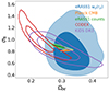Fig. 15.

Derived constraints on Ω_M and σ₈. Our result with the eRASS1 cluster clustering is shown in blue, the result from Planck Collaboration VI (2020, EEE TTT, lowL, lowE) in orange, the eRASS1 cluster abundance (Ghirardini et al. 2024) in green, CODEX (Lindholm et al. 2021) in red, and KiDS-DR3 (Lesci et al. 2022b) in violet.

The individual constraints from eRASS1 cluster clustering are not powerful enough to probe cosmological tensions such as the S8 or H₀ ones (Verde et al. 2019). The deeper data from future eRASS surveys will increase the number of clusters and reduce the uncertainty of the correlation function. Thanks to the combination with cluster counts (Ghirardini et al. 2024), eROSITA will measure cosmological parameters with per cent level accuracy (Merloni et al. 2012; Pillepich et al. 2018).

5. Conclusions

We summarise our results in Sect. 5.1 and provide a future outlook in Sect. 5.2.

5.1. Summary

The ability of eROSITA to effectively detect extended extra-galactic sources has yielded large samples of galaxy clusters. The eROSITA telescope observed 12 247 cluster candidates during its first all-sky survey (Bulbul et al. 2024; Kluge et al. 2024). Such a large sample is suitable for exploratory studies of their clustering, allowing us to learn about their distribution within the large-scale structure of the Universe and the dark matter halo population hosting such objects. In addition, clustering measurements provide individual cosmological constraints, independently from traditional cluster abundance experiments.

We studied the clustering of galaxy clusters detected in the first eROSITA all-sky survey (eRASS1). We generated a catalogue of random points that traces the same density and redshift distributions of the real data by construction, thanks to filtering according to the eRASS1 selection function (see Figs. 2 and 3). We applied a volume-limited selection in X-ray luminosity and redshift, by discarding clusters with L_X lower than that inferred from a reference flux F_X, lim = 4 × 10⁻¹⁴ erg s⁻¹ cm⁻² at the upper redshift limit of each sample. We obtained five different samples, whose properties are reported in Table 1. We measured the two-point autocorrelation function of each sample (see Eq. (1)). We computed covariance matrices by a jackknife method on the eRASS1 data and on a set of 1000 independent GLASS simulations (see Eq. (3) and Fig. 4).

We interpreted our measurement with a HOD approach (see Fig. 5). To our knowledge, this is the first attempt to constrain HOD parameters for X-ray selected clusters. We modelled the eRASS1 cluster incompleteness with the eRASS1 digital twin from Seppi et al. (2022). We found that bright clusters probe high-mass haloes, as expected. The M_min parameter shifts from 14.73 $_{- 0.35}^{+ 0.93}$ $^{+0.93}_{-0.35}$ for S0 to 15.04 $_{- 0.72}^{+ 0.61}$ $^{+0.61}_{-0.72}$ for S4. The large-scale halo bias consequently decreases from 4.34±0.62 for S4 to 2.95±0.21 for S0. We found that satellites populate a larger fraction of haloes in the low-luminosity samples. The M_sat parameter changes from 15.32 $_{- 0.33}^{+ 0.34}$ $^{+0.34}_{-0.33}$ to 15.76 $_{- 0.55}^{+ 0.42}$ $^{+0.42}_{-0.55}$ (see also Fig. 7). The high-mass samples prefer a sharp transition for central objects populating haloes, with $σ_{log M} = 0 . 57_{- 0.34}^{+ 0.29}$ $\sigma_{\log M} =0.57_{-0.34}^{+0.29}$ for S4. When probing lower-mass sources, eROSITA detects more satellite objects, and the transition is milder, with $σ_{log M} = 0 . 82_{- 0.49}^{+ 0.43}$ $\sigma_{\log M}=0.82_{-0.49}^{+0.43}$ for S0 (see Fig. 6 for the full posterior distribution). As a consequence, the fraction of satellites (Eq. (9)) reaches higher upper limits for low L_X samples (from < 8.1% to < 14.9%). The priors, posteriors, and derived HOD parameters are reported in Table 2. Using the best-fit HOD, we studied the relation between L_X and the bias in Fig. 8, and the scaling relation between L_X and M_500c in Fig. 10. The results agree with previous studies. We used a HAM approach to infer the scatter of X-ray luminosity at fixed halo mass, combining the five volume-limited samples we obtain ⟨σ_Lx⟩ = 0.36, in agreement with the literature. Our model agrees with measurements of the excess surface density obtained from the cross-correlation between the cluster positions and the galaxy shapes from KiDS data (Fig. A.1).

We focused on a larger flux-limited sample to study the cosmological implications of our clustering measurement. It consists of 6493 sources. We modelled the large-scale halo bias within the HOD framework without assuming a fiducial model. We followed the evolution mapping approach from Sánchez et al. (2022) and interpret our results in an h-independent way. We fixed all the cosmological parameters affecting the shape of the power spectrum, except for the physical cold dark matter density ω_c. We left the evolution parameters A_s and ω_DE free, together with M_min. We used the other HOD variables as nuisance parameters. We obtained constraints on $ω_{c} = 0 . 12_{- 0.02}^{+ 0.03}$ $\omega_{\mathrm{c}}=0.12^{+0.03}_{-0.02}$ and $σ_{12} = 0 . 77_{- 0.16}^{+ 0.22}$ $\sigma_{12}=0.77^{+0.22}_{-0.16}$ . The average bias of the flux-limited sample selected for cosmology is $b = 3 . 63_{- 0.85}^{+ 1.02}$ $b=3.63^{+1.02}_{-0.85}$ . We derived constraints on $Ω_{M} = 0 . 32_{- 0.03}^{+ 0.04}$ $\Omega_{\mathrm{M}}=0.32_{-0.03}^{+0.04}$ , $σ_{8} = 0 . 76_{- 0.16}^{+ 0.22}$ $\sigma_{8}=0.76^{+0.22}_{-0.16}$ . Our results are in excellent agreement with eRASS1 cluster abundance (Ghirardini et al. 2024). The full posterior distribution is shown in Fig. 14. Our results are compatible with similar clustering studies of galaxy clusters (Lindholm et al. 2021; Lesci et al. 2022b) and CMB (Planck Collaboration VI 2020).

5.2. Outlook

The future eROSITA all-sky surveys, thanks to the deeper data, will provide a more complete view of satellite groups to massive dark matter haloes, allowing us to probe clustering measurements on smaller scales and obtain better constraints on the satellite population from HOD modelling. Thanks to the development of new high-resolution mock Universes, a detailed comparison with simulations will then be possible. The next generation of cosmological simulations, such as FLAMINGO (Schaye et al. 2023), MilleniumTNG (Pakmor et al. 2023), and Cluster-TNG (Nelson et al. 2024), will help shed light on the fraction of satellites in the whole cluster population from the theoretical point of view.

A better understanding of the population of satellite haloes will also benefit from precise measurement and modelling of the subhalo mass function. From the perspective of simulations, the definition of a subhalo is not trivial. Diemer et al. (2023) show that traditional halo finders may fail in the subhalo identification due to tidal distortions and low particle resolution. They track subhalo particles in the simulations and obtain a better view of the whole subhalo population, which impacts the clustering measurements by more than 20% on small scales below 1 Mpc, also for haloes more massive than 10¹³ M_⊙. Such an approach will ultimately offer a more accurate prediction for the expected HOD parameters such as M_sat, α_sat, and the satellite fraction.

Another key ingredient for an accurate prediction of small-scale clustering is a reliable modelling of the additional suppression of the non-linear power spectrum due to baryons. Different works in the past few years provide ad hoc prescriptions from the comparison of dark matter-only simulations with parent runs including baryons, also as a function of the baryonic physics implementation (see e.g. Aricò et al. 2020; Salcido et al. 2023; Grandis et al. 2024).

Multiple works showed that the modelling of the excess surface density (ESD) improves the HOD modelling (see e.g. Comparat et al. 2023; More et al. 2023, for AGN and galaxies). Accurate models for clusters require accounting for mis-centring effects (Zhang et al. 2019), cluster member contamination (Varga et al. 2019), and redshift uncertainties (see discussion by Rykoff et al. 2014). Future developments in these areas will allow us to use ESD measurements not only as a consistency check (see Appendix A), but also as an additional term in the HOD likelihood together with clustering and improve the HOD constraints, making the best out of combined statistics for cosmological cluster studies (To et al. 2021).

Accurate and precise redshift measurements are key to studying the BAO feature using galaxies and clusters as probes of the large-scale structure (Comparat et al. 2013). The current quality provided by photometric redshifts is not sufficient (Kluge et al. 2024). In the future, spectroscopic follow-up of eROSITA clusters from SDSS-V (Kollmeier et al. 2017) and 4MOST (de Jong 2011; Finoguenov et al. 2019) will allow us to go beyond the measurement of projected clustering, enabling a detailed study of the 3D cluster clustering, redshift space distortions, and BAO modelling.

Clustering studies of the deeper eROSITA surveys such as eRASS:4 will allow us to fit cosmological parameters for different samples as a function of redshift, with better handling of the strong degeneracy between halo bias and clustering amplitude. An additional possibility is to model the bias externally, following traditional clustering studies in the literature (Marulli et al. 2018, 2021; Lesci et al. 2023). This approach relies on scaling relations and bias models, which could be a relevant source of systematic errors. However, a prior on the scaling relation parameters may come from cluster abundance, or a simultaneous fit of counts and clustering could constrain the scaling relations together with cosmological parameters, enhancing the cosmological results. With the HOD alone, our cosmological constraints are mild because a similar large-scale structure can be reproduced that has clusters residing in more massive haloes, within a Universe that produces more structures (i.e. with higher Ω_M and σ₈). The addition of optical cluster lensing, probing halo mass, may break this degeneracy and improve cosmological results. The simultaneous fitting of the clustering signal and the cluster abundance (Ghirardini et al. 2024) will allow an additional HOD constraint on the cluster number density, anchoring the clustering amplitude and partially solving the degeneracy with the halo bias. Similarly, the sensitivity to ω_DE will improve, together with the constraints on H₀. This will allow us to explore a larger portion of the cosmological parameter space and highlight the different degeneracy for the halo bias with σ₈ and σ₁₂. In addition, we will potentially go beyond the traditional ΛCDM model and provide constraints on primordial non-Gaussianity (Sartoris et al. 2010). We will explore these ideas in future work, which could benefit from updated alternatives to accurately predict the linear and non-linear power spectrum, such as the COMET package (Eggemeier et al. 2023). Additional HOD predictions may be possible by combining COMET with halomod (Murray et al. 2013, 2021). The development of emulators in recent years will allow a quick estimate of the likelihood for fitting purposes, and a comparison between different prescriptions will help in understanding systematic errors (see also DarkQuest and Sesame, Nishimichi et al. 2019; Mauland et al. 2024).

Finally, future studies with larger catalogues and higher number densities will require a precise estimate of the covariance matrix. The generation of end-to-end mocks is computationally very expensive. Such studies will benefit from fast and accurate estimates of the covariance matrix (Trusov et al. 2024), especially if the clustering is combined with external probes, such as cluster counts, where both experiments share common information (Fumagalli et al. 2024).

¹

The radius enclosing a total mass equal to 500 times the critical density of the Universe at the cluster’s redshift.

²

https://www.legacysurvey.org/dr10

³

https://www.legacysurvey.org/dr10/files/#random-catalogs-randoms

⁴

scipy, https://scipy.org/

⁵

https://corrfunc.readthedocs.io/

⁶

https://healpix.sourceforge.io/credits.php

⁷

https://scipy.org/

⁸

https://github.com/surhudm/aum

⁹

http://www.gnu.org/software/gsl

¹⁰

https://johannesbuchner.github.io/UltraNest/

¹¹

https://getdist.readthedocs.io/en/latest/

¹²

https://dsigma.readthedocs.io

Acknowledgments

R. Seppi thanks S. More for advice on the AUM software. N.C. is supported by CNES. This work is based on data from eROSITA, the soft X-ray instrument aboard SRG, a joint Russian-German science mission supported by the Russian Space Agency (Roskosmos), in the interests of the Russian Academy of Sciences represented by its Space Research Institute (IKI), and the Deutsches Zentrum für Luft- und Raumfahrt (DLR). The SRG spacecraft was built by Lavochkin Association (NPOL) and its subcontractors, and is operated by NPOL with support from the Max Planck Institute for Extraterrestrial Physics (MPE). The development and construction of the eROSITA X-ray instrument was led by MPE, with contributions from the Dr. Karl Remeis Observatory Bamberg & ECAP (FAU Erlangen-Nuernberg), the University of Hamburg Observatory, the Leibniz Institute for Astrophysics Potsdam (AIP), and the Institute for Astronomy and Astrophysics of the University of Tübingen, with the support of DLR and the Max Planck Society. The Argelander Institute for Astronomy of the University of Bonn and the Ludwig Maximilians Universität Munich also participated in the science preparation for eROSITA. The eROSITA data shown here were processed using the eSASS/NRTA software system developed by the German eROSITA consortium. Based on observations made with ESO Telescopes at the La Silla Paranal Observatory under programme IDs 177.A-3016, 177.A-3017, 177.A-3018 and 179.A-2004, and on data products produced by the KiDS consortium. The KiDS production team acknowledges support from: Deutsche Forschungsgemeinschaft, ERC, NOVA and NWO-M grants; Target; the University of Padova, and the University Federico II (Naples).

References

Abbott, T. M. C., Aguena, M., Alarcon, A., et al. 2022, Phys. Rev. D, 105, 023520 [CrossRef] [Google Scholar]
Adami, C., Giles, P., Koulouridis, E., et al. 2018, A&A, 620, A5 [NASA ADS] [CrossRef] [EDP Sciences] [Google Scholar]
Alam, S., Aubert, M., Avila, S., et al. 2021, Phys. Rev. D, 103, 083533 [NASA ADS] [CrossRef] [Google Scholar]
Alcock, C., & Paczynski, B. 1979, Nature, 281, 358 [NASA ADS] [CrossRef] [Google Scholar]
Allen, S. W., Evrard, A. E., & Mantz, A. B. 2011, ARA&A, 49, 409 [Google Scholar]
Angulo, R. E., & Hahn, O. 2022, Liv. Rev. Comput. Astrophys., 8, 1 [CrossRef] [Google Scholar]
Angulo, R. E., Zennaro, M., Contreras, S., et al. 2021, MNRAS, 507, 5869 [NASA ADS] [CrossRef] [Google Scholar]
Aricò, G., Angulo, R. E., Hernández-Monteagudo, C., et al. 2020, MNRAS, 495, 4800 [Google Scholar]
Arnaud, K. A. 1996, in Astronomical Data Analysis Software and Systems V, eds. G. H. Jacoby, & J. Barnes, ASP Conf. Ser., 101, 17 [NASA ADS] [Google Scholar]
Artis, E., Ghirardini, V., Bulbul, E., et al. 2024, A&A, submitted [arXiv:2402.08459] [Google Scholar]
Asgari, M., Mead, A. J., & Heymans, C. 2023, Open J. Astrophys., 6, 39 [NASA ADS] [CrossRef] [Google Scholar]
Balaguera-Antolínez, A., Sánchez, A. G., Böhringer, H., et al. 2011, MNRAS, 413, 386 [NASA ADS] [CrossRef] [Google Scholar]
Bardeen, J. M., Bond, J. R., Kaiser, N., & Szalay, A. S. 1986, ApJ, 304, 15 [Google Scholar]
Bartelmann, M., & Schneider, P. 2001, Phys. Rep., 340, 291 [Google Scholar]
Baugh, C. M., & Efstathiou, G. 1993, MNRAS, 265, 145 [NASA ADS] [CrossRef] [Google Scholar]
Berlind, A. A., & Weinberg, D. H. 2002, ApJ, 575, 587 [Google Scholar]
Bhattacharya, S., Heitmann, K., White, M., et al. 2011, ApJ, 732, 122 [NASA ADS] [CrossRef] [Google Scholar]
Bocquet, S., Dietrich, J. P., Schrabback, T., et al. 2019, ApJ, 878, 55 [Google Scholar]
Borgani, S., Plionis, M., & Kolokotronis, V. 1999, MNRAS, 305, 866 [NASA ADS] [CrossRef] [Google Scholar]
Brunner, H., Liu, T., Lamer, G., et al. 2022, A&A, 661, A1 [NASA ADS] [CrossRef] [EDP Sciences] [Google Scholar]
Buchner, J. 2016, Stat. Comput., 26, 383 [Google Scholar]
Buchner, J. 2019, PASP, 131, 108005 [Google Scholar]
Buchner, J. 2021, J. Open Source Softw., 6, 3001 [CrossRef] [Google Scholar]
Bulbul, E., Chiu, I. N., Mohr, J. J., et al. 2019, ApJ, 871, 50 [Google Scholar]
Bulbul, E., Liu, A., Kluge, M., et al. 2024, A&A, 685, A106 [NASA ADS] [CrossRef] [EDP Sciences] [Google Scholar]
Capasso, R., Mohr, J. J., Saro, A., et al. 2020, MNRAS, 494, 2736 [CrossRef] [Google Scholar]
Chiu, I. N., Ghirardini, V., Liu, A., et al. 2022, A&A, 661, A11 [NASA ADS] [CrossRef] [EDP Sciences] [Google Scholar]
Clerc, N., & Finoguenov, A. 2023, in Handbook of X-ray and Gamma-ray Astrophysics, eds. C. Bambi,& A. Santangelo (Springer Living Reference Work), 123 [Google Scholar]
Clerc, N., Ramos-Ceja, M. E., Ridl, J., et al. 2018, A&A, 617, A92 [NASA ADS] [CrossRef] [EDP Sciences] [Google Scholar]
Clerc, N., Comparat, J., Seppi, R., et al. 2024, A&A, in press, https://doi.org/10.1051/0004-6361/202449447 [Google Scholar]
Coil, A. L. 2013, in Planets, Stars and Stellar Systems. Volume 6: Extragalactic Astronomy and Cosmology, eds. T. D. Oswalt, & W. C. Keel, 6, 387 [NASA ADS] [CrossRef] [Google Scholar]
Comparat, J., Jullo, E., Kneib, J.-P., et al. 2013, MNRAS, 433, 1146 [Google Scholar]
Comparat, J., Prada, F., Yepes, G., & Klypin, A. 2017, MNRAS, 469, 4157 [NASA ADS] [CrossRef] [Google Scholar]
Comparat, J., Eckert, D., Finoguenov, A., et al. 2020, Open J. Astrophys., 3, 13 [Google Scholar]
Comparat, J., Luo, W., Merloni, A., et al. 2023, A&A, 673, A122 [NASA ADS] [CrossRef] [EDP Sciences] [Google Scholar]
Costanzi, M., Saro, A., Bocquet, S., et al. 2021, Phys. Rev. D, 103, 043522 [Google Scholar]
Davis, M., & Peebles, P. J. E. 1983, ApJ, 267, 465 [Google Scholar]
de Jong, R. 2011, The Messenger, 145, 14 [NASA ADS] [Google Scholar]
Despali, G., Giocoli, C., Angulo, R. E., et al. 2016, MNRAS, 456, 2486 [NASA ADS] [CrossRef] [Google Scholar]
Dey, A., Schlegel, D. J., Lang, D., et al. 2019, AJ, 157, 168 [Google Scholar]
Diemer, B., Behroozi, P., & Mansfield, P. 2023, arXiv e-prints [arXiv:2305.00993] [Google Scholar]
Dolag, K., Borgani, S., Murante, G., & Springel, V. 2009, MNRAS, 399, 497 [Google Scholar]
Eggemeier, A., Camacho-Quevedo, B., Pezzotta, A., et al. 2023, MNRAS, 519, 2962 [Google Scholar]
Eisenstein, D. J., & Hu, W. 1998, ApJ, 496, 605 [Google Scholar]
Elvin-Poole, J., Crocce, M., Ross, A. J., et al. 2018, Phys. Rev. D, 98, 042006 [Google Scholar]
Favole, G., Comparat, J., Prada, F., et al. 2016, MNRAS, 461, 3421 [NASA ADS] [CrossRef] [Google Scholar]
Finoguenov, A., Merloni, A., Comparat, J., et al. 2019, The Messenger, 175, 39 [NASA ADS] [Google Scholar]
Finoguenov, A., Rykoff, E., Clerc, N., et al. 2020, A&A, 638, A114 [NASA ADS] [CrossRef] [EDP Sciences] [Google Scholar]
Fisher, K. B., Davis, M., Strauss, M. A., Yahil, A., & Huchra, J. 1994, MNRAS, 266, 50 [NASA ADS] [CrossRef] [Google Scholar]
Fumagalli, A., Biagetti, M., Saro, A., et al. 2022, JCAP, 2022, 022 [CrossRef] [Google Scholar]
Fumagalli, A., Costanzi, M., Saro, A., Castro, T., & Borgani, S. 2024, A&A, 682, A148 [NASA ADS] [CrossRef] [EDP Sciences] [Google Scholar]
Garrel, C., Pierre, M., Valageas, P., et al. 2022, A&A, 663, A3 [NASA ADS] [CrossRef] [EDP Sciences] [Google Scholar]
Georgakakis, A., Nandra, K., Laird, E. S., Aird, J., & Trichas, M. 2008, MNRAS, 388, 1205 [Google Scholar]
Ghirardini, V., Bulbul, E., Artis, E., et al. 2024, A&A, submitted [arXiv:2402.08458] [Google Scholar]
Grandis, S., Bocquet, S., Mohr, J. J., Klein, M., & Dolag, K. 2021, MNRAS, 507, 5671 [NASA ADS] [CrossRef] [Google Scholar]
Grandis, S., Aricò, G., Schneider, A., & Linke, L. 2024, MNRAS, 528, 4379 [NASA ADS] [CrossRef] [Google Scholar]
Guo, H., Zheng, Z., Behroozi, P. S., et al. 2016, MNRAS, 459, 3040 [NASA ADS] [CrossRef] [Google Scholar]
Guo, H., Yang, X., Raichoor, A., et al. 2019, ApJ, 871, 147 [NASA ADS] [CrossRef] [Google Scholar]
Hamilton, A. J. S. 1992, ApJ, 385, L5 [NASA ADS] [CrossRef] [Google Scholar]
Hamilton, A. J. S. 1993, ApJ, 417, 19 [Google Scholar]
Hamilton, A. J. S. 2000, MNRAS, 312, 257 [NASA ADS] [CrossRef] [Google Scholar]
Heymans, C., Tröster, T., Asgari, M., et al. 2021, A&A, 646, A140 [NASA ADS] [CrossRef] [EDP Sciences] [Google Scholar]
HI4PI Collaboration (Ben Bekhti, N., et al.) 2016, A&A, 594, A116 [NASA ADS] [CrossRef] [EDP Sciences] [Google Scholar]
Hogg, D. W. 1999, arXiv e-prints [arXiv:astro-ph/9905116] [Google Scholar]
Hong, T., Han, J. L., & Wen, Z. L. 2016, ApJ, 826, 154 [NASA ADS] [CrossRef] [Google Scholar]
Ider Chitham, J., Comparat, J., Finoguenov, A., et al. 2020, MNRAS, 499, 4768 [NASA ADS] [CrossRef] [Google Scholar]
Ingoglia, L., Covone, G., Sereno, M., et al. 2022, MNRAS, 511, 1484 [NASA ADS] [CrossRef] [Google Scholar]
Jackson, J. C. 1972, MNRAS, 156, 1P [CrossRef] [Google Scholar]
Jeong, D., Dai, L., Kamionkowski, M., & Szalay, A. S. 2015, MNRAS, 449, 3312 [NASA ADS] [CrossRef] [Google Scholar]
Kaiser, N. 1987, MNRAS, 227, 1 [Google Scholar]
Kluge, M., Comparat, J., Liu, A., et al. 2024, A&A, submitted [arXiv:2402.08453] [Google Scholar]
Klypin, A., & Prada, F. 2018, MNRAS, 478, 4602 [NASA ADS] [CrossRef] [Google Scholar]
Klypin, A. A., Trujillo-Gomez, S., & Primack, J. 2011, ApJ, 740, 102 [NASA ADS] [CrossRef] [Google Scholar]
Klypin, A., Yepes, G., Gottlöber, S., Prada, F., & Heß, S. 2016, MNRAS, 457, 4340 [Google Scholar]
Kollmeier, J. A., Zasowski, G., Rix, H.-W., et al. 2017, arXiv e-prints [arXiv:1711.03234] [Google Scholar]
Kravtsov, A. V., & Borgani, S. 2012, ARA&A, 50, 353 [Google Scholar]
Kravtsov, A. V., Berlind, A. A., Wechsler, R. H., et al. 2004, ApJ, 609, 35 [Google Scholar]
Krumpe, M., Miyaji, T., & Coil, A. L. 2010, ApJ, 713, 558 [NASA ADS] [CrossRef] [Google Scholar]
Krumpe, M., Miyaji, T., Husemann, B., et al. 2015, ApJ, 815, 21 [NASA ADS] [CrossRef] [Google Scholar]
Krumpe, M., Miyaji, T., Georgakakis, A., et al. 2023, ApJ, 952, 109 [NASA ADS] [CrossRef] [Google Scholar]
Kuijken, K., Heymans, C., Dvornik, A., et al. 2019, A&A, 625, A2 [NASA ADS] [CrossRef] [EDP Sciences] [Google Scholar]
Lacey, C., & Cole, S. 1993, MNRAS, 262, 627 [NASA ADS] [CrossRef] [Google Scholar]
Landy, S. D., & Szalay, A. S. 1993, ApJ, 412, 64 [Google Scholar]
Lange, J., & Huang, S. 2022, Astrophysics Source Code Library [record ascl:2204.006] [Google Scholar]
Lesci, G. F., Marulli, F., Moscardini, L., et al. 2022a, A&A, 659, A88 [NASA ADS] [CrossRef] [EDP Sciences] [Google Scholar]
Lesci, G. F., Nanni, L., Marulli, F., et al. 2022b, A&A, 665, A100 [NASA ADS] [CrossRef] [EDP Sciences] [Google Scholar]
Lesci, G. F., Veropalumbo, A., Sereno, M., et al. 2023, A&A, 674, A80 [NASA ADS] [CrossRef] [EDP Sciences] [Google Scholar]
Lewis, A. 2019, arXiv e-prints [arXiv:1910.13970] [Google Scholar]
Lindholm, V., Finoguenov, A., Comparat, J., et al. 2021, A&A, 646, A8 [NASA ADS] [CrossRef] [EDP Sciences] [Google Scholar]
Liu, A., Bulbul, E., Ghirardini, V., et al. 2022, A&A, 661, A2 [NASA ADS] [CrossRef] [EDP Sciences] [Google Scholar]
Liu, A., Bulbul, E., Kluge, M., et al. 2024, A&A, 683, A130 [NASA ADS] [CrossRef] [EDP Sciences] [Google Scholar]
Lovisari, L., Reiprich, T. H., & Schellenberger, G. 2015, A&A, 573, A118 [NASA ADS] [CrossRef] [EDP Sciences] [Google Scholar]
Lovisari, L., Schellenberger, G., Sereno, M., et al. 2020, ApJ, 892, 102 [Google Scholar]
Maller, A. H., McIntosh, D. H., Katz, N., & Weinberg, M. D. 2005, ApJ, 619, 147 [NASA ADS] [CrossRef] [Google Scholar]
Mana, A., Giannantonio, T., Weller, J., et al. 2013, MNRAS, 434, 684 [NASA ADS] [CrossRef] [Google Scholar]
Mandelbaum, R., Tasitsiomi, A., Seljak, U., Kravtsov, A. V., & Wechsler, R. H. 2005, MNRAS, 362, 1451 [NASA ADS] [CrossRef] [Google Scholar]
Mantz, A. B., von der Linden, A., Allen, S. W., et al. 2015, MNRAS, 446, 2205 [Google Scholar]
Mantz, A. B., Allen, S. W., Morris, R. G., et al. 2016, MNRAS, 463, 3582 [NASA ADS] [CrossRef] [Google Scholar]
Marulli, F., Veropalumbo, A., Moscardini, L., Cimatti, A., & Dolag, K. 2017, A&A, 599, A106 [NASA ADS] [CrossRef] [EDP Sciences] [Google Scholar]
Marulli, F., Veropalumbo, A., Sereno, M., et al. 2018, A&A, 620, A1 [NASA ADS] [CrossRef] [EDP Sciences] [Google Scholar]
Marulli, F., Veropalumbo, A., García-Farieta, J. E., et al. 2021, ApJ, 920, 13 [Google Scholar]
Mauland, R., Winther, H. A., & Ruan, C.-Z. 2024, A&A, 685, A156 [NASA ADS] [CrossRef] [EDP Sciences] [Google Scholar]
McClintock, T., Varga, T. N., Gruen, D., et al. 2019, MNRAS, 482, 1352 [Google Scholar]
Merloni, A., Predehl, P., Becker, W., et al. 2012, arXiv e-prints [arXiv:1209.3114] [Google Scholar]
Merloni, A., Lamer, G., Liu, T., et al. 2024, A&A, 682, A34 [NASA ADS] [CrossRef] [EDP Sciences] [Google Scholar]
Mo, H. J., & White, S. D. M. 1996, MNRAS, 282, 347 [Google Scholar]
More, S. 2021, Astrophysics Source Code Library [record ascl:2108.002] [Google Scholar]
More, S., Miyatake, H., Mandelbaum, R., et al. 2015, ApJ, 806, 2 [CrossRef] [Google Scholar]
More, S., Sugiyama, S., Miyatake, H., et al. 2023, Phys. Rev. D, 108, 123520 [NASA ADS] [CrossRef] [Google Scholar]
Moscardini, L., Matarrese, S., De Grandi, S., & Lucchin, F. 2000, MNRAS, 314, 647 [NASA ADS] [CrossRef] [Google Scholar]
Murray, S. G., Power, C., & Robotham, A. S. G. 2013, Astron. Comput., 3, 23 [CrossRef] [Google Scholar]
Murray, S. G., Diemer, B., Chen, Z., et al. 2021, Astron. Comput., 36, 100487 [NASA ADS] [CrossRef] [Google Scholar]
Nelson, D., Pillepich, A., Ayromlou, M., et al. 2024, A&A, 686, A157 [NASA ADS] [CrossRef] [EDP Sciences] [Google Scholar]
Nishimichi, T., Takada, M., Takahashi, R., et al. 2019, ApJ, 884, 29 [NASA ADS] [CrossRef] [Google Scholar]
Norberg, P., Baugh, C. M., Gaztañaga, E., & Croton, D. J. 2009, MNRAS, 396, 19 [Google Scholar]
Pakmor, R., Springel, V., Coles, J. P., et al. 2023, MNRAS, 524, 2539 [NASA ADS] [CrossRef] [Google Scholar]
Peacock, J. A., & Smith, R. E. 2000, MNRAS, 318, 1144 [Google Scholar]
Peacock, J. A., Cole, S., Norberg, P., et al. 2001, Nature, 410, 169 [Google Scholar]
Percival, W. J., & White, M. 2009, MNRAS, 393, 297 [NASA ADS] [CrossRef] [Google Scholar]
Pillepich, A., Reiprich, T. H., Porciani, C., Borm, K., & Merloni, A. 2018, MNRAS, 481, 613 [Google Scholar]
Planck Collaboration XIII. 2016, A&A, 594, A13 [NASA ADS] [CrossRef] [EDP Sciences] [Google Scholar]
Planck Collaboration VI. 2020, A&A, 641, A6 [NASA ADS] [CrossRef] [EDP Sciences] [Google Scholar]
Pratt, G. W., Croston, J. H., Arnaud, M., & Böhringer, H. 2009, A&A, 498, 361 [NASA ADS] [CrossRef] [EDP Sciences] [Google Scholar]
Pratt, G. W., Arnaud, M., Biviano, A., et al. 2019, Space Sci. Rev., 215, 25 [Google Scholar]
Predehl, P., Andritschke, R., Arefiev, V., et al. 2021, A&A, 647, A1 [EDP Sciences] [Google Scholar]
Ragagnin, A., Saro, A., Singh, P., & Dolag, K. 2021, MNRAS, 500, 5056 [Google Scholar]
Rocher, A., Ruhlmann-Kleider, V., Burtin, E., & de Mattia, A. 2023, JCAP, 2023, 033 [CrossRef] [Google Scholar]
Rodríguez-Torres, S. A., Chuang, C.-H., Prada, F., et al. 2016, MNRAS, 460, 1173 [CrossRef] [Google Scholar]
Rodríguez-Torres, S. A., Comparat, J., Prada, F., et al. 2017, MNRAS, 468, 728 [CrossRef] [Google Scholar]
Romanello, M., Marulli, F., Moscardini, L., et al. 2024, A&A, 682, A72 [NASA ADS] [CrossRef] [EDP Sciences] [Google Scholar]
Rykoff, E. S., Rozo, E., Busha, M. T., et al. 2014, ApJ, 785, 104 [Google Scholar]
Rykoff, E. S., Rozo, E., Hollowood, D., et al. 2016, ApJS, 224, 1 [NASA ADS] [CrossRef] [Google Scholar]
Salcedo, A. N., Weinberg, D. H., Wu, H.-Y., & Wibking, B. D. 2022, MNRAS, 510, 5376 [CrossRef] [Google Scholar]
Salcido, J., McCarthy, I. G., Kwan, J., Upadhye, A., & Font, A. S. 2023, MNRAS, 523, 2247 [NASA ADS] [CrossRef] [Google Scholar]
Sánchez, A. G. 2020, Phys. Rev. D, 102, 123511 [CrossRef] [Google Scholar]
Sánchez, A. G., Ruiz, A. N., Jara, J. G., & Padilla, N. D. 2022, MNRAS, 514, 5673 [CrossRef] [Google Scholar]
Sartoris, B., Borgani, S., Fedeli, C., et al. 2010, MNRAS, 407, 2339 [Google Scholar]
Sartoris, B., Biviano, A., Fedeli, C., et al. 2016, MNRAS, 459, 1764 [Google Scholar]
Schaye, J., Kugel, R., Schaller, M., et al. 2023, MNRAS, 526, 4978 [NASA ADS] [CrossRef] [Google Scholar]
Schellenberger, G., & Reiprich, T. H. 2017, MNRAS, 469, 3738 [CrossRef] [Google Scholar]
Schrabback, T., Bocquet, S., Sommer, M., et al. 2021, MNRAS, 505, 3923 [NASA ADS] [CrossRef] [Google Scholar]
Scoccimarro, R., Couchman, H. M. P., & Frieman, J. A. 1999, ApJ, 517, 531 [NASA ADS] [CrossRef] [Google Scholar]
Semenaite, A., Sánchez, A. G., Pezzotta, A., et al. 2022, MNRAS, 512, 5657 [NASA ADS] [CrossRef] [Google Scholar]
Seppi, R., Comparat, J., Nandra, K., et al. 2021, A&A, 652, A155 [NASA ADS] [CrossRef] [EDP Sciences] [Google Scholar]
Seppi, R., Comparat, J., Bulbul, E., et al. 2022, A&A, 665, A78 [NASA ADS] [CrossRef] [EDP Sciences] [Google Scholar]
Sheth, R. K., & Tormen, G. 1999, MNRAS, 308, 119 [Google Scholar]
Sheth, R. K., Mo, H. J., & Tormen, G. 2001, MNRAS, 323, 1 [NASA ADS] [CrossRef] [Google Scholar]
Sinha, M., & Garrison, L. 2019, in Software Challenges to Exascale Computing, eds. A. Majumdar, & R. Arora (Singapore: Springer), 3 [NASA ADS] [CrossRef] [Google Scholar]
Sinha, M., & Garrison, L. H. 2020, MNRAS, 491, 3022 [Google Scholar]
Smith, R. E., Peacock, J. A., Jenkins, A., et al. 2003, MNRAS, 341, 1311 [Google Scholar]
Sunayama, T., Miyatake, H., Sugiyama, S., et al. 2023, arXiv e-prints [arXiv:2309.13025] [Google Scholar]
Tessore, N., Loureiro, A., Joachimi, B., von Wietersheim-Kramsta, M., & Jeffrey, N. 2023, Open J. Astrophys., 6, 11 [NASA ADS] [CrossRef] [Google Scholar]
Tinker, J., Kravtsov, A. V., Klypin, A., et al. 2008, ApJ, 688, 709 [Google Scholar]
Tinker, J. L., Robertson, B. E., Kravtsov, A. V., et al. 2010, ApJ, 724, 878 [NASA ADS] [CrossRef] [Google Scholar]
To, C., Krause, E., Rozo, E., et al. 2021, Phys. Rev. Lett., 126, 141301 [NASA ADS] [CrossRef] [Google Scholar]
Trusov, S., Zarrouk, P., Cole, S., et al. 2024, MNRAS, 527, 9048 [Google Scholar]
Umetsu, K. 2020, A&ARv, 28, 7 [Google Scholar]
Valageas, P., & Clerc, N. 2012, A&A, 547, A100 [NASA ADS] [CrossRef] [EDP Sciences] [Google Scholar]
van den Bosch, F. C., More, S., Cacciato, M., Mo, H., & Yang, X. 2013, MNRAS, 430, 725 [NASA ADS] [CrossRef] [Google Scholar]
Varga, T. N., DeRose, J., Gruen, D., et al. 2019, MNRAS, 489, 2511 [NASA ADS] [CrossRef] [Google Scholar]
Verde, L., Treu, T., & Riess, A. G. 2019, Nat. Astron., 3, 891 [Google Scholar]
Veropalumbo, A., Marulli, F., Moscardini, L., Moresco, M., & Cimatti, A. 2016, MNRAS, 458, 1909 [NASA ADS] [CrossRef] [Google Scholar]
Virtanen, P., Gommers, R., Oliphant, T. E., et al. 2020, Nat. Meth., 17, 261 [Google Scholar]
Zehavi, I., Zheng, Z., Weinberg, D. H., et al. 2005, ApJ, 630, 1 [Google Scholar]
Zehavi, I., Zheng, Z., Weinberg, D. H., et al. 2011, ApJ, 736, 59 [NASA ADS] [CrossRef] [Google Scholar]
Zhang, Y., Jeltema, T., Hollowood, D. L., et al. 2019, MNRAS, 487, 2578 [NASA ADS] [CrossRef] [Google Scholar]
Zheng, Z., Berlind, A. A., Weinberg, D. H., et al. 2005, ApJ, 633, 791 [NASA ADS] [CrossRef] [Google Scholar]
Zheng, Z., Coil, A. L., & Zehavi, I. 2007, ApJ, 667, 760 [Google Scholar]
Zhou, R., Newman, J. A., Mao, Y.-Y., et al. 2021, MNRAS, 501, 3309 [NASA ADS] [CrossRef] [Google Scholar]
Zu, Y., & Mandelbaum, R. 2015, MNRAS, 454, 1161 [Google Scholar]

Appendix A: Optical Cluster Lensing

As a consistency check, we test our HOD model against a measurement of the excess surface density from optical cluster lensing. The latter is a cross-correlation between clusters acting as foreground lenses at redshift z_l and the shape of background galaxies acting as sources at redshift z_s (Bartelmann & Schneider 2001). The principle is the same as galaxy-galaxy lensing (Mandelbaum et al. 2005), but in our case, the lens is a cluster and not a galaxy. We use the galaxy shapes from the Kilo Degree Survey (KiDS) DR4 (Kuijken et al. 2019). The cross-correlation with lensing encodes the difference between the mean density within a given aperture and the density at the aperture location. This quantity is named excess surface density ΔΣ (or ESD). It is related to the galaxy-matter correlation function by Eq. A.1:

$\begin{matrix} Σ (R) & = \bar{ρ_{m}} \int ξ_{gm} (\sqrt{R^{2} + π^{2}}) d π, \\ Δ Σ & = \bar{Σ (< R)} - Σ (R) = Σ_{crit} γ (R), \end{matrix}$ $\begin{aligned} \Sigma (R)&= \overline{\rho _m} \int \xi _{gm}(\sqrt{R^2+\pi ^2})d\pi ,\nonumber \\ \Delta \Sigma&= \overline{\Sigma ( < R)} - \Sigma (R) = \Sigma _{\rm crit}\gamma (R), \end{aligned}$ (A.1)

where $Σ_{crit} = \frac{c^{2}}{4 π G} \frac{D_{A} (z_{s})}{D_{A} (z_{l}) D_{A} (z_{s}, z_{l})} \frac{1}{{(1 + z_{l})}^{2}}$ $\Sigma_{\mathrm{crit}}=\dfrac{c^2}{4\pi G} \dfrac{D_{\mathrm{A}}(z_s)}{D_{\mathrm{A}}(z_l)D_{\mathrm{A}}(z_s,z_l)}\dfrac{1}{(1+z_l)^2}$ is the critical surface density, which depends on the angular angular diameter distances between the lens and the source planes, and γ(R) is the cluster shear profile. We measure ΔΣ with the publicly available dsigma software¹² (Lange & Huang 2022). The excess surface density is estimated according to:

$\begin{matrix} Δ Σ = \frac{\sum_{ls} w_{ls} Σ_{crit} (z_{l}, z_{s}) e_{t}}{\sum_{ls} w_{ls}}, \end{matrix}$ $\begin{aligned} \Delta \Sigma = \frac{\sum _{ls} { w}_{ls} \Sigma _{\rm crit}(z_l,z_s) e_t}{\sum _{ls} { w}_{ls}}, \end{aligned}$ (A.2)

where e_t is the source tangential ellipticity, w_s is a source weight that minimises shape noise, and $w_{ls} = \frac{w_{s}}{Σ_{crit}^{2} (z_{l}, z_{s})}$ $\mathit{w}_{ls}=\dfrac{\mathit{w}_s}{\Sigma^2_{\mathrm{crit}}(z_l,z_s)}$ .

We focus on the redshift range 0.1 < z < 0.3. We require the redshift of background sources to be z_s > z_l + 0.1. The model is evaluated at the average redshift of each cluster sample acting as a lens. The result is shown in Fig. A.1. It shows the measurement of KiDS data with error bars. The prediction by our HOD model is shown by the solid lines, with 1-σ and 2-σ uncertainty denoted by the shaded areas. Overall, we find a good agreement between the data and the prediction. We conclude that our HOD model is consistent with optical cluster lensing measurements. In future studies, accounting for mis-centring, cluster member contamination, and photo-z uncertainties, in ESD models for clusters will allow us to use this quantity to improve the HOD constraining power for clusters (see Comparat et al. 2023, for AGN).

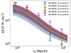Fig. A.1.

Excess surface density as a function of radial separation measured around eRASS1 clusters with KiDS data. The prediction from our best-fit HOD model is shown by the solid lines. The shaded areas denote the 1-σ and 2-σ confidence in the prediction. Each colour denotes one of the volume-limited samples (see Table 1).

Appendix B: Systematics

In this Appendix, we evaluate the impact of possible systematic effects on our results. We consider the covariance matrix, the photometric redshifts, and the choice of the priors.

B.1. Covariance Matrix

The jackknife estimate of the covariance matrix for our study provides noisy off-diagonal terms, that do not properly capture the proper correlation between different radial bins of the correlation function (Klypin & Prada 2018; Fumagalli et al. 2022). Therefore, we used independent GLASS simulations to estimate the off-diagonal terms of the covariance matrix, as explained in Sect. 3. Although these simulations reproduce the average source density of the eRASS1 cluster sample, they do not account for the exact survey geometry of eRASS1. Running a large number of independent end-to-end mocks similar to the one presented in (Seppi et al. 2022) is computationally unfeasible for this work. In this Appendix, we test the impact of the off-diagonal terms of the covariance on our results by comparing the standard analysis to an additional case where we only use the diagonal elements estimated from the jackknife method as errors. The likelihood reads:

$\begin{matrix} log L = - \frac{1}{2} {(\frac{D - M (θ)}{σ})}^{2}, \end{matrix}$ $\begin{aligned} \log \mathcal{L} = - \frac{1}{2}\left(\dfrac{\mathbf{D }-\mathbf{M }(\theta )}{\sigma }\right)^2, \end{aligned}$ (B.1)

where D is the data array for the projected correlation function, M is the w_p(r_p) model that depends on the array of parameters θ, and the error is an array obtained from the diagonal elements of the covariance matrix $σ = \sqrt{C_{ii}}$ $\sigma = \sqrt{C_{ii}}$ . The result is reported in Table B.1. There is excellent agreement between the best-fit values obtained from the diagonal likelihood in Eq. B.1 to the standard analysis. Like in the previous section, the α_sat parameter is the most sensitive, changing by about 4% from 1.41 $_{- 0.58}^{+ 0.82}$ $^{+0.82}_{-0.58}$ in the standard analysis to 1.47 $_{- 0.60}^{+ 0.83}$ $^{+0.83}_{-0.60}$ for the diagonal error one. The values are well-compatible within uncertainties. The full marginalised posterior distribution is shown in Fig. B.1. We conclude that estimating the off-diagonal elements of the covariance matrix with simulations that do not account for exact survey specifications does not have a significant impact on our results for this study.

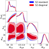Fig. B.1.

Comparison between the marginalised posterior distributions of the best fit HOD parameters on the S2 sample and the diagonal error case. The filled 2D contours show the 1-σ and 2-σ confidence levels of the posteriors after convolution with the uniform priors. The model is given by Eq. 8. The corresponding 1D parameter constraints are reported in Table B.1. The blue (red) shaded area denotes the standard (diagonal error) case.

Table B.1.

Priors and posteriors of the HOD and the derived parameters for the test about the choice of the priors.

B.2. Impact of photometric redshift

The optical follow-up of eRASS1 clusters provides an excellent measurement of photometric redshift, with a 0.5% scatter around spectroscopic values (Kluge et al. 2024). The authors also show that the uncertainty is independent of redshift in our range of interest 0.1 < z < 0.6. Nonetheless, we test the impact of using photometric redshift for the distance conversion in the measurement of the projected correlation function.

Following the procedure explained in Sect. 3, we compute the projected correlation function of the eRASS1 mock from Seppi et al. (2022) for the flux-limited sample spanning 0.1 < z < 0.6, the selection is explained in Sect. 2.1. At first, we use the spectroscopic redshifts in the simulation for distance conversions and measure the true w_p, T. Secondly, we mock photometric redshifts in the simulation by adding a normal scatter of F × (1 + z) to the spec-z. We consider three values of the factor F equal to 0.005, which is the eRASS1 case, but also worse-case scenarios of 0.01 and 0.02. We measure a w_p, F for each one. For each set of correlation functions measured with different F factors, we compute its median distribution, and its 16th and 84th percentiles.

The result is shown in Fig. B.2. The black points show the measurement using spec-z, and the error bars are derived from the diagonal elements of the covariance matrix (see Sect. 3). The blue, orange, and green lines denote the mock photo-z cases with different levels of degradation. The shaded areas include the 16th and 84th percentiles of the 100 tests. The tests corresponding to σ_z = 0.5% and σ_z = 1% are in excellent agreement with the spec-z case. The worst-case scenario of σ_z = 2% shows a noticeable offset instead. We infer the relative shift of the correlation function due to the redshift error as

$\begin{matrix} E = \frac{w_{p, T} - w_{p, F}}{w_{p, T}} \cdot \end{matrix}$ $\begin{aligned} E = \frac{{ w}_{\rm p,T} - { w}_{\rm p,F}}{{ w}_{\rm p,T}}\cdot \end{aligned}$ (B.2)

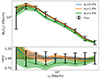Fig. B.2.

Projected correlation function measured on a flux-limited sample selected from the eRASS1 mock by Seppi et al. (2022), in the range 0.1 < z < 0.6, following the selection scheme explained in Sect. 3. The black points show the measurement using spectroscopic redshifts in the simulation. The blue, orange, and green lines denote three tests where the redshift was degraded to mock a photo-z, by adding a scatter of σ_z × (1 + z) around the spec-z. The bottom panel shows the ratio to the spectroscopic redshift case.

For the three F factors equal to 0.5%, 1%, and 2%, we respectively obtain median shifts of E equal to 1.7%, 2.3%, and 10.5%. The covariance matrix gives an average relative uncertainty of 15.3%. We conclude that redshift errors have a minimal impact on our measurement, especially for the eRASS1 case with 0.5% scatter. For future eROSITA all-sky surveys with deeper data, the precision of the correlation function measurement may be comparable to the dilution of the clustering signal due to photometric redshift. In that case, the redshift error should be carefully considered in the modelling. In particular, it could bias the normalisation of the correlation function due to its potential degeneracy with the clustering amplitude.

B.3. Choice of the priors

The posteriors obtained from the HOD analysis in Fig. 6 are non-Gaussian. This is due to the intrinsic correlation and degeneracy between HOD parameters, but specific choices of the prior may also contribute to this aspect. Therefore, we test whether our HOD results are affected by the choice of the priors. We consider the S2 sample defined in Table 1 and fit the correlation function with the HOD model and methodology described in Sect. 3. On top of the standard prior used for the analysis (see also Table 2), we test two additional sets of priors, with larger and smaller uniform distributions.

The priors and the corresponding posteriors for each case are reported in Table B.1. The best-fit values of the parameters inferred from the median of the posterior distribution, together with the 16th and 84th percentiles, are compatible between the three choices of the prior. In particular, there is excellent agreement between the standard analysis and the larger prior one. The α_sat parameter is the most sensitive one, changing by about 6% from 1.45 $_{- 0.61}^{+ 0.86}$ $^{+0.86}_{-0.61}$ for the large prior to 1.35 $_{- 0.50}^{+ 0.67}$ $^{+0.67}_{-0.50}$ for the small prior choice. The difference is well within uncertainties. The full marginalised posterior distributions for the three experiments are shown in Fig. B.3. The posterior from the standard analysis recovers well the 1-σ distribution of the large prior case. Instead, the small prior case is not able to fully explore the 1-σ posterior distribution of the standard and large prior analysis. We deduce that the standard set of priors chosen for this analysis does not have a strong impact on our results.

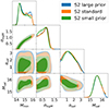Fig. B.3.

Marginalised posterior distributions of the best-fit HOD parameters on the S2 sample with different choices of the priors. The filled 2D contours show the 1-σ and 2-σ confidence levels of the posteriors after convolution with the uniform priors. The model is given by Eq. 8. The corresponding one-dimensional parameter constraints are reported in Table B.1. The blue (orange, green) shaded area denotes the large (standard, small) prior case.

All Tables

Table 1.

Properties of the volume-limited eRASS1 cluster samples for our clustering study.

In the text

Table 2.

Priors and posteriors for the HOD and the derived parameters on the five volume-limited eRASS1 samples (see Table 1 and Fig. 1).

In the text

Table 3.

Optimal values of the scatter parameter σ_HAM for each volume-limited sample.

In the text

Table 4.

Priors and posteriors on the cosmology and large-scale halo bias parameters.

In the text

Table B.1.

Priors and posteriors of the HOD and the derived parameters for the test about the choice of the priors.

In the text

All Figures

	Fig. 1. Volume-limited selection of the eRASS1 cluster sample for our clustering study as a function of X-ray luminosity and redshift. The full sample is shown in cyan; the five subsamples are denoted in blue, orange, green, red, and pink.
In the text

	Fig. 2. Angular distribution of the selected eRASS:1 clusters (top panel) and the random points (bottom panel), after the application of the masks. The points are colour-coded according to their normalised local density. The density of the random catalogue changes through the sky very similarly to the eRASS1 data.
In the text

Fig. 3.

Probability density redshift distribution of the selected eRASS:1 clusters and the random points. The panel shows the total number of clusters (randoms) in each redshift bin divided by the size of the bin in blue (orange), normalised by the integral over the redshift range. Two black vertical lines denote the redshift range used in our analysis, between 0.1 and 0.6. The bump in redshift at about 0.8 is due to a filter transition in the measurement of photo-z (see Kluge et al. 2024).

In the text

	Fig. 4. Jackknife correlation matrix C_i, j/ $\sqrt{C_{i, i} C_{j, j}}$ $\sqrt{C_{i,i}C_{j,j}}$ for the projected correlation function of the eRASS1 cluster sample described in Sect. 2. The covariance matrix for the different samples presented in Sect. 2.1 is computed via jackknife (see Eq. (4)).
In the text

	Fig. 5. Projected correlation functions of the volume selected eRASS1 clusters samples. Each colour denotes one sample. The error bars show the measurement, the solid line is the best fit model, and the shaded areas denote the 1-σ and 2-σ uncertainty on the model. For clarity, we shift the measurements and models by e^{0, 1, 2, 3, 4} from S0 to S4.
In the text

	Fig. 6. Marginalised posterior distributions of the best fit HOD parameters. The filled 2D contours show the 1-σ and 2-σ confidence levels of the posteriors after convolution with the uniform priors. The model is given by Eq. (8). The corresponding 1D parameter constraints are reported in Table 2.
In the text

	Fig. 7. Derived distribution of the eRASS1 clusters and groups population in dark matter haloes (solid lines), divided in central (dashed) and satellite (dotted) objects. The colours denote each volume-limited sample (see Table 1). The shaded areas denote the 1-σ confidence levels on the model. For clarity, only the S0 and S4 samples are shown.
In the text

	Fig. 8. Large-scale halo bias as a function of average X-ray luminosity for the eRASS1 volume-limited samples. Each point is colour-coded by the average redshift of the sample. The black line shows the best-fit linear relation.
In the text

Fig. 9.

Comparison between the halo bias of eRASS1 clusters (in blue) with other experiments and probes from Planck clusters in orange (Lesci et al. 2023), CODEX clusters in green (Lindholm et al. 2021), XXL clusters in red (Marulli et al. 2018), DES-Y1 clusters in purple (Rykoff et al. 2016), eFEDS AGN in brown (Comparat et al. 2023), RASS AGN in pink (Krumpe et al. 2015), DES-Y1 galaxies in grey (Elvin-Poole et al. 2018), DES-Y3 galaxies in yellow (Abbott et al. 2022), and SDSS-DR7 galaxies selected in stellar mass in cyan (Zu & Mandelbaum 2015).

In the text

Fig. 10.

Scaling relation between halo mass and X-ray luminosity. The halo mass is inferred from our best-fit HOD (in blue). The black line shows a linear fit to our data points. The green dots denote a collection of clusters from Lovisari et al. (2015, 2020), Mantz et al. (2016), Schellenberger & Reiprich (2017), Adami et al. (2018), Bulbul et al. (2019), and Liu et al. (2022). The eRASS1 sample is denoted in red (Bulbul et al. 2024). The shaded area includes a scatter σ_Lx = 0.36 around the mean relation, obtained by the halo abundance matching explained in Sect. 4.2. The extrapolated scaling relation outside the parameter space sensitive to our HOD approach is indicated with the dashed black line and the hatched shaded area.

In the text

Fig. 11.

Comparison between the HOD results from Sect. 4.1 and the abundance matching procedure. The top panels show the prediction for the number of central objects as a function of mass, the bottom panels show the projected correlation function. For clarity, only 9 of the 100 HAM predictions are shown. The panels on the left refer to the S0 sample and the ones on the right to the S4 one. The shaded areas denote the results and measurements from the data; the coloured lines show the HAM predictions with different values of the scatter σ_HAM.

In the text

	Fig. 12. Projected correlation functions of the eRASS1 clusters. The error bars show the measurement, the solid line is the best fit cosmological model, and the shaded areas denote the 1-σ and 2-σ uncertainty on the model.
In the text

	Fig. 13. Marginalised posterior distributions of the best-fit cosmological parameters. The 1-σ and 2-σ confidence levels of the posteriors are shown as filled 2D contours. The model is explained in Sect. 3.1.2. The parameters are reported in Table 4.
In the text

Fig. 14.

Marginalised posterior distributions of the best-fit cosmological parameters. The 1-σ and 2-σ confidence levels of the posteriors are shown as filled 2D contours. The model is explained in Sect. 3.1.2. The parameters are reported in Table 4. The left panel shows h-independent parameters: the physical cold dark matter density ω_c, the clustering amplitude σ₁₂, and the physical dark energy density ω_DE. The right panel shows the traditional inferred parameters: the matter density Ω_M, the amplitude σ₈ and the Hubble constant H₀. The constraints from the flux-limited eRASS1 sample are shown in blue, the CMB results from Planck Collaboration VI (2020) in orange.

In the text

	Fig. 15. Derived constraints on Ω_M and σ₈. Our result with the eRASS1 cluster clustering is shown in blue, the result from Planck Collaboration VI (2020, EEE TTT, lowL, lowE) in orange, the eRASS1 cluster abundance (Ghirardini et al. 2024) in green, CODEX (Lindholm et al. 2021) in red, and KiDS-DR3 (Lesci et al. 2022b) in violet.
In the text

	Fig. A.1. Excess surface density as a function of radial separation measured around eRASS1 clusters with KiDS data. The prediction from our best-fit HOD model is shown by the solid lines. The shaded areas denote the 1-σ and 2-σ confidence in the prediction. Each colour denotes one of the volume-limited samples (see Table 1).
In the text

Fig. B.1.

Comparison between the marginalised posterior distributions of the best fit HOD parameters on the S2 sample and the diagonal error case. The filled 2D contours show the 1-σ and 2-σ confidence levels of the posteriors after convolution with the uniform priors. The model is given by Eq. 8. The corresponding 1D parameter constraints are reported in Table B.1. The blue (red) shaded area denotes the standard (diagonal error) case.

In the text

Fig. B.2.

Projected correlation function measured on a flux-limited sample selected from the eRASS1 mock by Seppi et al. (2022), in the range 0.1 < z < 0.6, following the selection scheme explained in Sect. 3. The black points show the measurement using spectroscopic redshifts in the simulation. The blue, orange, and green lines denote three tests where the redshift was degraded to mock a photo-z, by adding a scatter of σ_z × (1 + z) around the spec-z. The bottom panel shows the ratio to the spectroscopic redshift case.

In the text

Fig. B.3.

Marginalised posterior distributions of the best-fit HOD parameters on the S2 sample with different choices of the priors. The filled 2D contours show the 1-σ and 2-σ confidence levels of the posteriors after convolution with the uniform priors. The model is given by Eq. 8. The corresponding one-dimensional parameter constraints are reported in Table B.1. The blue (orange, green) shaded area denotes the large (standard, small) prior case.

In the text

Current usage metrics show cumulative count of Article Views (full-text article views including HTML views, PDF and ePub downloads, according to the available data) and Abstracts Views on Vision4Press platform.

Data correspond to usage on the plateform after 2015. The current usage metrics is available 48-96 hours after online publication and is updated daily on week days.

Initial download of the metrics may take a while.

[1] Abbott, T. M. C., Aguena, M., Alarcon, A., et al. 2022, Phys. Rev. D, 105, 023520 [CrossRef] [Google Scholar]

[2] Adami, C., Giles, P., Koulouridis, E., et al. 2018, A&A, 620, A5 [NASA ADS] [CrossRef] [EDP Sciences] [Google Scholar]

[3] Alam, S., Aubert, M., Avila, S., et al. 2021, Phys. Rev. D, 103, 083533 [NASA ADS] [CrossRef] [Google Scholar]

[4] Alcock, C., & Paczynski, B. 1979, Nature, 281, 358 [NASA ADS] [CrossRef] [Google Scholar]

[5] Allen, S. W., Evrard, A. E., & Mantz, A. B. 2011, ARA&A, 49, 409 [Google Scholar]

[6] Angulo, R. E., & Hahn, O. 2022, Liv. Rev. Comput. Astrophys., 8, 1 [CrossRef] [Google Scholar]

[7] Angulo, R. E., Zennaro, M., Contreras, S., et al. 2021, MNRAS, 507, 5869 [NASA ADS] [CrossRef] [Google Scholar]

[8] Aricò, G., Angulo, R. E., Hernández-Monteagudo, C., et al. 2020, MNRAS, 495, 4800 [Google Scholar]

[9] Arnaud, K. A. 1996, in Astronomical Data Analysis Software and Systems V, eds. G. H. Jacoby, & J. Barnes, ASP Conf. Ser., 101, 17 [NASA ADS] [Google Scholar]

[10] Artis, E., Ghirardini, V., Bulbul, E., et al. 2024, A&A, submitted [arXiv:2402.08459] [Google Scholar]

[11] Asgari, M., Mead, A. J., & Heymans, C. 2023, Open J. Astrophys., 6, 39 [NASA ADS] [CrossRef] [Google Scholar]

[12] Balaguera-Antolínez, A., Sánchez, A. G., Böhringer, H., et al. 2011, MNRAS, 413, 386 [NASA ADS] [CrossRef] [Google Scholar]

[13] Bardeen, J. M., Bond, J. R., Kaiser, N., & Szalay, A. S. 1986, ApJ, 304, 15 [Google Scholar]

[14] Bartelmann, M., & Schneider, P. 2001, Phys. Rep., 340, 291 [Google Scholar]

[15] Baugh, C. M., & Efstathiou, G. 1993, MNRAS, 265, 145 [NASA ADS] [CrossRef] [Google Scholar]

[16] Berlind, A. A., & Weinberg, D. H. 2002, ApJ, 575, 587 [Google Scholar]

[17] Bhattacharya, S., Heitmann, K., White, M., et al. 2011, ApJ, 732, 122 [NASA ADS] [CrossRef] [Google Scholar]

[18] Bocquet, S., Dietrich, J. P., Schrabback, T., et al. 2019, ApJ, 878, 55 [Google Scholar]

[19] Borgani, S., Plionis, M., & Kolokotronis, V. 1999, MNRAS, 305, 866 [NASA ADS] [CrossRef] [Google Scholar]

[20] Brunner, H., Liu, T., Lamer, G., et al. 2022, A&A, 661, A1 [NASA ADS] [CrossRef] [EDP Sciences] [Google Scholar]

[21] Buchner, J. 2016, Stat. Comput., 26, 383 [Google Scholar]

[22] Buchner, J. 2019, PASP, 131, 108005 [Google Scholar]

[23] Buchner, J. 2021, J. Open Source Softw., 6, 3001 [CrossRef] [Google Scholar]

[24] Bulbul, E., Chiu, I. N., Mohr, J. J., et al. 2019, ApJ, 871, 50 [Google Scholar]

[25] Bulbul, E., Liu, A., Kluge, M., et al. 2024, A&A, 685, A106 [NASA ADS] [CrossRef] [EDP Sciences] [Google Scholar]

[26] Capasso, R., Mohr, J. J., Saro, A., et al. 2020, MNRAS, 494, 2736 [CrossRef] [Google Scholar]

[27] Chiu, I. N., Ghirardini, V., Liu, A., et al. 2022, A&A, 661, A11 [NASA ADS] [CrossRef] [EDP Sciences] [Google Scholar]

[28] Clerc, N., & Finoguenov, A. 2023, in Handbook of X-ray and Gamma-ray Astrophysics, eds. C. Bambi,& A. Santangelo (Springer Living Reference Work), 123 [Google Scholar]

[29] Clerc, N., Ramos-Ceja, M. E., Ridl, J., et al. 2018, A&A, 617, A92 [NASA ADS] [CrossRef] [EDP Sciences] [Google Scholar]

[30] Clerc, N., Comparat, J., Seppi, R., et al. 2024, A&A, in press, https://doi.org/10.1051/0004-6361/202449447 [Google Scholar]

[31] Coil, A. L. 2013, in Planets, Stars and Stellar Systems. Volume 6: Extragalactic Astronomy and Cosmology, eds. T. D. Oswalt, & W. C. Keel, 6, 387 [NASA ADS] [CrossRef] [Google Scholar]

[32] Comparat, J., Jullo, E., Kneib, J.-P., et al. 2013, MNRAS, 433, 1146 [Google Scholar]

[33] Comparat, J., Prada, F., Yepes, G., & Klypin, A. 2017, MNRAS, 469, 4157 [NASA ADS] [CrossRef] [Google Scholar]

[34] Comparat, J., Eckert, D., Finoguenov, A., et al. 2020, Open J. Astrophys., 3, 13 [Google Scholar]

[35] Comparat, J., Luo, W., Merloni, A., et al. 2023, A&A, 673, A122 [NASA ADS] [CrossRef] [EDP Sciences] [Google Scholar]

[36] Costanzi, M., Saro, A., Bocquet, S., et al. 2021, Phys. Rev. D, 103, 043522 [Google Scholar]

[37] Davis, M., & Peebles, P. J. E. 1983, ApJ, 267, 465 [Google Scholar]

[38] de Jong, R. 2011, The Messenger, 145, 14 [NASA ADS] [Google Scholar]

[39] Despali, G., Giocoli, C., Angulo, R. E., et al. 2016, MNRAS, 456, 2486 [NASA ADS] [CrossRef] [Google Scholar]

[40] Dey, A., Schlegel, D. J., Lang, D., et al. 2019, AJ, 157, 168 [Google Scholar]

[41] Diemer, B., Behroozi, P., & Mansfield, P. 2023, arXiv e-prints [arXiv:2305.00993] [Google Scholar]

[42] Dolag, K., Borgani, S., Murante, G., & Springel, V. 2009, MNRAS, 399, 497 [Google Scholar]

[43] Eggemeier, A., Camacho-Quevedo, B., Pezzotta, A., et al. 2023, MNRAS, 519, 2962 [Google Scholar]

[44] Eisenstein, D. J., & Hu, W. 1998, ApJ, 496, 605 [Google Scholar]

[45] Elvin-Poole, J., Crocce, M., Ross, A. J., et al. 2018, Phys. Rev. D, 98, 042006 [Google Scholar]

[46] Favole, G., Comparat, J., Prada, F., et al. 2016, MNRAS, 461, 3421 [NASA ADS] [CrossRef] [Google Scholar]

[47] Finoguenov, A., Merloni, A., Comparat, J., et al. 2019, The Messenger, 175, 39 [NASA ADS] [Google Scholar]

[48] Finoguenov, A., Rykoff, E., Clerc, N., et al. 2020, A&A, 638, A114 [NASA ADS] [CrossRef] [EDP Sciences] [Google Scholar]

[49] Fisher, K. B., Davis, M., Strauss, M. A., Yahil, A., & Huchra, J. 1994, MNRAS, 266, 50 [NASA ADS] [CrossRef] [Google Scholar]

[50] Fumagalli, A., Biagetti, M., Saro, A., et al. 2022, JCAP, 2022, 022 [CrossRef] [Google Scholar]

[51] Fumagalli, A., Costanzi, M., Saro, A., Castro, T., & Borgani, S. 2024, A&A, 682, A148 [NASA ADS] [CrossRef] [EDP Sciences] [Google Scholar]

[52] Garrel, C., Pierre, M., Valageas, P., et al. 2022, A&A, 663, A3 [NASA ADS] [CrossRef] [EDP Sciences] [Google Scholar]

[53] Georgakakis, A., Nandra, K., Laird, E. S., Aird, J., & Trichas, M. 2008, MNRAS, 388, 1205 [Google Scholar]

[54] Ghirardini, V., Bulbul, E., Artis, E., et al. 2024, A&A, submitted [arXiv:2402.08458] [Google Scholar]

[55] Grandis, S., Bocquet, S., Mohr, J. J., Klein, M., & Dolag, K. 2021, MNRAS, 507, 5671 [NASA ADS] [CrossRef] [Google Scholar]

[56] Grandis, S., Aricò, G., Schneider, A., & Linke, L. 2024, MNRAS, 528, 4379 [NASA ADS] [CrossRef] [Google Scholar]

[57] Guo, H., Zheng, Z., Behroozi, P. S., et al. 2016, MNRAS, 459, 3040 [NASA ADS] [CrossRef] [Google Scholar]

[58] Guo, H., Yang, X., Raichoor, A., et al. 2019, ApJ, 871, 147 [NASA ADS] [CrossRef] [Google Scholar]

[59] Hamilton, A. J. S. 1992, ApJ, 385, L5 [NASA ADS] [CrossRef] [Google Scholar]

[60] Hamilton, A. J. S. 1993, ApJ, 417, 19 [Google Scholar]

[61] Hamilton, A. J. S. 2000, MNRAS, 312, 257 [NASA ADS] [CrossRef] [Google Scholar]

[62] Heymans, C., Tröster, T., Asgari, M., et al. 2021, A&A, 646, A140 [NASA ADS] [CrossRef] [EDP Sciences] [Google Scholar]

[63] HI4PI Collaboration (Ben Bekhti, N., et al.) 2016, A&A, 594, A116 [NASA ADS] [CrossRef] [EDP Sciences] [Google Scholar]

[64] Hogg, D. W. 1999, arXiv e-prints [arXiv:astro-ph/9905116] [Google Scholar]

[65] Hong, T., Han, J. L., & Wen, Z. L. 2016, ApJ, 826, 154 [NASA ADS] [CrossRef] [Google Scholar]

[66] Ider Chitham, J., Comparat, J., Finoguenov, A., et al. 2020, MNRAS, 499, 4768 [NASA ADS] [CrossRef] [Google Scholar]

[67] Ingoglia, L., Covone, G., Sereno, M., et al. 2022, MNRAS, 511, 1484 [NASA ADS] [CrossRef] [Google Scholar]

[68] Jackson, J. C. 1972, MNRAS, 156, 1P [CrossRef] [Google Scholar]

[69] Jeong, D., Dai, L., Kamionkowski, M., & Szalay, A. S. 2015, MNRAS, 449, 3312 [NASA ADS] [CrossRef] [Google Scholar]

[70] Kaiser, N. 1987, MNRAS, 227, 1 [Google Scholar]

[71] Kluge, M., Comparat, J., Liu, A., et al. 2024, A&A, submitted [arXiv:2402.08453] [Google Scholar]

[72] Klypin, A., & Prada, F. 2018, MNRAS, 478, 4602 [NASA ADS] [CrossRef] [Google Scholar]

[73] Klypin, A. A., Trujillo-Gomez, S., & Primack, J. 2011, ApJ, 740, 102 [NASA ADS] [CrossRef] [Google Scholar]

[74] Klypin, A., Yepes, G., Gottlöber, S., Prada, F., & Heß, S. 2016, MNRAS, 457, 4340 [Google Scholar]

[75] Kollmeier, J. A., Zasowski, G., Rix, H.-W., et al. 2017, arXiv e-prints [arXiv:1711.03234] [Google Scholar]

[76] Kravtsov, A. V., & Borgani, S. 2012, ARA&A, 50, 353 [Google Scholar]

[77] Kravtsov, A. V., Berlind, A. A., Wechsler, R. H., et al. 2004, ApJ, 609, 35 [Google Scholar]

[78] Krumpe, M., Miyaji, T., & Coil, A. L. 2010, ApJ, 713, 558 [NASA ADS] [CrossRef] [Google Scholar]

[79] Krumpe, M., Miyaji, T., Husemann, B., et al. 2015, ApJ, 815, 21 [NASA ADS] [CrossRef] [Google Scholar]

[80] Krumpe, M., Miyaji, T., Georgakakis, A., et al. 2023, ApJ, 952, 109 [NASA ADS] [CrossRef] [Google Scholar]

[81] Kuijken, K., Heymans, C., Dvornik, A., et al. 2019, A&A, 625, A2 [NASA ADS] [CrossRef] [EDP Sciences] [Google Scholar]

[82] Lacey, C., & Cole, S. 1993, MNRAS, 262, 627 [NASA ADS] [CrossRef] [Google Scholar]

[83] Landy, S. D., & Szalay, A. S. 1993, ApJ, 412, 64 [Google Scholar]

[84] Lange, J., & Huang, S. 2022, Astrophysics Source Code Library [record ascl:2204.006] [Google Scholar]

[85] Lesci, G. F., Marulli, F., Moscardini, L., et al. 2022a, A&A, 659, A88 [NASA ADS] [CrossRef] [EDP Sciences] [Google Scholar]

[86] Lesci, G. F., Nanni, L., Marulli, F., et al. 2022b, A&A, 665, A100 [NASA ADS] [CrossRef] [EDP Sciences] [Google Scholar]

[87] Lesci, G. F., Veropalumbo, A., Sereno, M., et al. 2023, A&A, 674, A80 [NASA ADS] [CrossRef] [EDP Sciences] [Google Scholar]

[88] Lewis, A. 2019, arXiv e-prints [arXiv:1910.13970] [Google Scholar]

[89] Lindholm, V., Finoguenov, A., Comparat, J., et al. 2021, A&A, 646, A8 [NASA ADS] [CrossRef] [EDP Sciences] [Google Scholar]

[90] Liu, A., Bulbul, E., Ghirardini, V., et al. 2022, A&A, 661, A2 [NASA ADS] [CrossRef] [EDP Sciences] [Google Scholar]

[91] Liu, A., Bulbul, E., Kluge, M., et al. 2024, A&A, 683, A130 [NASA ADS] [CrossRef] [EDP Sciences] [Google Scholar]

[92] Lovisari, L., Reiprich, T. H., & Schellenberger, G. 2015, A&A, 573, A118 [NASA ADS] [CrossRef] [EDP Sciences] [Google Scholar]

[93] Lovisari, L., Schellenberger, G., Sereno, M., et al. 2020, ApJ, 892, 102 [Google Scholar]

[94] Maller, A. H., McIntosh, D. H., Katz, N., & Weinberg, M. D. 2005, ApJ, 619, 147 [NASA ADS] [CrossRef] [Google Scholar]

[95] Mana, A., Giannantonio, T., Weller, J., et al. 2013, MNRAS, 434, 684 [NASA ADS] [CrossRef] [Google Scholar]

[96] Mandelbaum, R., Tasitsiomi, A., Seljak, U., Kravtsov, A. V., & Wechsler, R. H. 2005, MNRAS, 362, 1451 [NASA ADS] [CrossRef] [Google Scholar]

[97] Mantz, A. B., von der Linden, A., Allen, S. W., et al. 2015, MNRAS, 446, 2205 [Google Scholar]

[98] Mantz, A. B., Allen, S. W., Morris, R. G., et al. 2016, MNRAS, 463, 3582 [NASA ADS] [CrossRef] [Google Scholar]

[99] Marulli, F., Veropalumbo, A., Moscardini, L., Cimatti, A., & Dolag, K. 2017, A&A, 599, A106 [NASA ADS] [CrossRef] [EDP Sciences] [Google Scholar]

[100] Marulli, F., Veropalumbo, A., Sereno, M., et al. 2018, A&A, 620, A1 [NASA ADS] [CrossRef] [EDP Sciences] [Google Scholar]

[101] Marulli, F., Veropalumbo, A., García-Farieta, J. E., et al. 2021, ApJ, 920, 13 [Google Scholar]

[102] Mauland, R., Winther, H. A., & Ruan, C.-Z. 2024, A&A, 685, A156 [NASA ADS] [CrossRef] [EDP Sciences] [Google Scholar]

[103] McClintock, T., Varga, T. N., Gruen, D., et al. 2019, MNRAS, 482, 1352 [Google Scholar]

[104] Merloni, A., Predehl, P., Becker, W., et al. 2012, arXiv e-prints [arXiv:1209.3114] [Google Scholar]

[105] Merloni, A., Lamer, G., Liu, T., et al. 2024, A&A, 682, A34 [NASA ADS] [CrossRef] [EDP Sciences] [Google Scholar]

[106] Mo, H. J., & White, S. D. M. 1996, MNRAS, 282, 347 [Google Scholar]

[107] More, S. 2021, Astrophysics Source Code Library [record ascl:2108.002] [Google Scholar]

[108] More, S., Miyatake, H., Mandelbaum, R., et al. 2015, ApJ, 806, 2 [CrossRef] [Google Scholar]

[109] More, S., Sugiyama, S., Miyatake, H., et al. 2023, Phys. Rev. D, 108, 123520 [NASA ADS] [CrossRef] [Google Scholar]

[110] Moscardini, L., Matarrese, S., De Grandi, S., & Lucchin, F. 2000, MNRAS, 314, 647 [NASA ADS] [CrossRef] [Google Scholar]

[111] Murray, S. G., Power, C., & Robotham, A. S. G. 2013, Astron. Comput., 3, 23 [CrossRef] [Google Scholar]

[112] Murray, S. G., Diemer, B., Chen, Z., et al. 2021, Astron. Comput., 36, 100487 [NASA ADS] [CrossRef] [Google Scholar]

[113] Nelson, D., Pillepich, A., Ayromlou, M., et al. 2024, A&A, 686, A157 [NASA ADS] [CrossRef] [EDP Sciences] [Google Scholar]

[114] Nishimichi, T., Takada, M., Takahashi, R., et al. 2019, ApJ, 884, 29 [NASA ADS] [CrossRef] [Google Scholar]

[115] Norberg, P., Baugh, C. M., Gaztañaga, E., & Croton, D. J. 2009, MNRAS, 396, 19 [Google Scholar]

[116] Pakmor, R., Springel, V., Coles, J. P., et al. 2023, MNRAS, 524, 2539 [NASA ADS] [CrossRef] [Google Scholar]

[117] Peacock, J. A., & Smith, R. E. 2000, MNRAS, 318, 1144 [Google Scholar]

[118] Peacock, J. A., Cole, S., Norberg, P., et al. 2001, Nature, 410, 169 [Google Scholar]

[119] Percival, W. J., & White, M. 2009, MNRAS, 393, 297 [NASA ADS] [CrossRef] [Google Scholar]

[120] Pillepich, A., Reiprich, T. H., Porciani, C., Borm, K., & Merloni, A. 2018, MNRAS, 481, 613 [Google Scholar]

[121] Planck Collaboration XIII. 2016, A&A, 594, A13 [NASA ADS] [CrossRef] [EDP Sciences] [Google Scholar]

[122] Planck Collaboration VI. 2020, A&A, 641, A6 [NASA ADS] [CrossRef] [EDP Sciences] [Google Scholar]

[123] Pratt, G. W., Croston, J. H., Arnaud, M., & Böhringer, H. 2009, A&A, 498, 361 [NASA ADS] [CrossRef] [EDP Sciences] [Google Scholar]

[124] Pratt, G. W., Arnaud, M., Biviano, A., et al. 2019, Space Sci. Rev., 215, 25 [Google Scholar]

[125] Predehl, P., Andritschke, R., Arefiev, V., et al. 2021, A&A, 647, A1 [EDP Sciences] [Google Scholar]

[126] Ragagnin, A., Saro, A., Singh, P., & Dolag, K. 2021, MNRAS, 500, 5056 [Google Scholar]

[127] Rocher, A., Ruhlmann-Kleider, V., Burtin, E., & de Mattia, A. 2023, JCAP, 2023, 033 [CrossRef] [Google Scholar]

[128] Rodríguez-Torres, S. A., Chuang, C.-H., Prada, F., et al. 2016, MNRAS, 460, 1173 [CrossRef] [Google Scholar]

[129] Rodríguez-Torres, S. A., Comparat, J., Prada, F., et al. 2017, MNRAS, 468, 728 [CrossRef] [Google Scholar]

[130] Romanello, M., Marulli, F., Moscardini, L., et al. 2024, A&A, 682, A72 [NASA ADS] [CrossRef] [EDP Sciences] [Google Scholar]

[131] Rykoff, E. S., Rozo, E., Busha, M. T., et al. 2014, ApJ, 785, 104 [Google Scholar]

[132] Rykoff, E. S., Rozo, E., Hollowood, D., et al. 2016, ApJS, 224, 1 [NASA ADS] [CrossRef] [Google Scholar]

[133] Salcedo, A. N., Weinberg, D. H., Wu, H.-Y., & Wibking, B. D. 2022, MNRAS, 510, 5376 [CrossRef] [Google Scholar]

[134] Salcido, J., McCarthy, I. G., Kwan, J., Upadhye, A., & Font, A. S. 2023, MNRAS, 523, 2247 [NASA ADS] [CrossRef] [Google Scholar]

[135] Sánchez, A. G. 2020, Phys. Rev. D, 102, 123511 [CrossRef] [Google Scholar]

[136] Sánchez, A. G., Ruiz, A. N., Jara, J. G., & Padilla, N. D. 2022, MNRAS, 514, 5673 [CrossRef] [Google Scholar]

[137] Sartoris, B., Borgani, S., Fedeli, C., et al. 2010, MNRAS, 407, 2339 [Google Scholar]

[138] Sartoris, B., Biviano, A., Fedeli, C., et al. 2016, MNRAS, 459, 1764 [Google Scholar]

[139] Schaye, J., Kugel, R., Schaller, M., et al. 2023, MNRAS, 526, 4978 [NASA ADS] [CrossRef] [Google Scholar]

[140] Schellenberger, G., & Reiprich, T. H. 2017, MNRAS, 469, 3738 [CrossRef] [Google Scholar]

[141] Schrabback, T., Bocquet, S., Sommer, M., et al. 2021, MNRAS, 505, 3923 [NASA ADS] [CrossRef] [Google Scholar]

[142] Scoccimarro, R., Couchman, H. M. P., & Frieman, J. A. 1999, ApJ, 517, 531 [NASA ADS] [CrossRef] [Google Scholar]

[143] Semenaite, A., Sánchez, A. G., Pezzotta, A., et al. 2022, MNRAS, 512, 5657 [NASA ADS] [CrossRef] [Google Scholar]

[144] Seppi, R., Comparat, J., Nandra, K., et al. 2021, A&A, 652, A155 [NASA ADS] [CrossRef] [EDP Sciences] [Google Scholar]

[145] Seppi, R., Comparat, J., Bulbul, E., et al. 2022, A&A, 665, A78 [NASA ADS] [CrossRef] [EDP Sciences] [Google Scholar]

[146] Sheth, R. K., & Tormen, G. 1999, MNRAS, 308, 119 [Google Scholar]

[147] Sheth, R. K., Mo, H. J., & Tormen, G. 2001, MNRAS, 323, 1 [NASA ADS] [CrossRef] [Google Scholar]

[148] Sinha, M., & Garrison, L. 2019, in Software Challenges to Exascale Computing, eds. A. Majumdar, & R. Arora (Singapore: Springer), 3 [NASA ADS] [CrossRef] [Google Scholar]

[149] Sinha, M., & Garrison, L. H. 2020, MNRAS, 491, 3022 [Google Scholar]

[150] Smith, R. E., Peacock, J. A., Jenkins, A., et al. 2003, MNRAS, 341, 1311 [Google Scholar]

[151] Sunayama, T., Miyatake, H., Sugiyama, S., et al. 2023, arXiv e-prints [arXiv:2309.13025] [Google Scholar]

[152] Tessore, N., Loureiro, A., Joachimi, B., von Wietersheim-Kramsta, M., & Jeffrey, N. 2023, Open J. Astrophys., 6, 11 [NASA ADS] [CrossRef] [Google Scholar]

[153] Tinker, J., Kravtsov, A. V., Klypin, A., et al. 2008, ApJ, 688, 709 [Google Scholar]

[154] Tinker, J. L., Robertson, B. E., Kravtsov, A. V., et al. 2010, ApJ, 724, 878 [NASA ADS] [CrossRef] [Google Scholar]

[155] To, C., Krause, E., Rozo, E., et al. 2021, Phys. Rev. Lett., 126, 141301 [NASA ADS] [CrossRef] [Google Scholar]

[156] Trusov, S., Zarrouk, P., Cole, S., et al. 2024, MNRAS, 527, 9048 [Google Scholar]

[157] Umetsu, K. 2020, A&ARv, 28, 7 [Google Scholar]

[158] Valageas, P., & Clerc, N. 2012, A&A, 547, A100 [NASA ADS] [CrossRef] [EDP Sciences] [Google Scholar]

[159] van den Bosch, F. C., More, S., Cacciato, M., Mo, H., & Yang, X. 2013, MNRAS, 430, 725 [NASA ADS] [CrossRef] [Google Scholar]

[160] Varga, T. N., DeRose, J., Gruen, D., et al. 2019, MNRAS, 489, 2511 [NASA ADS] [CrossRef] [Google Scholar]

[161] Verde, L., Treu, T., & Riess, A. G. 2019, Nat. Astron., 3, 891 [Google Scholar]

[162] Veropalumbo, A., Marulli, F., Moscardini, L., Moresco, M., & Cimatti, A. 2016, MNRAS, 458, 1909 [NASA ADS] [CrossRef] [Google Scholar]

[163] Virtanen, P., Gommers, R., Oliphant, T. E., et al. 2020, Nat. Meth., 17, 261 [Google Scholar]

[164] Zehavi, I., Zheng, Z., Weinberg, D. H., et al. 2005, ApJ, 630, 1 [Google Scholar]

[165] Zehavi, I., Zheng, Z., Weinberg, D. H., et al. 2011, ApJ, 736, 59 [NASA ADS] [CrossRef] [Google Scholar]

[166] Zhang, Y., Jeltema, T., Hollowood, D. L., et al. 2019, MNRAS, 487, 2578 [NASA ADS] [CrossRef] [Google Scholar]

[167] Zheng, Z., Berlind, A. A., Weinberg, D. H., et al. 2005, ApJ, 633, 791 [NASA ADS] [CrossRef] [Google Scholar]

[168] Zheng, Z., Coil, A. L., & Zehavi, I. 2007, ApJ, 667, 760 [Google Scholar]

[169] Zhou, R., Newman, J. A., Mao, Y.-Y., et al. 2021, MNRAS, 501, 3309 [NASA ADS] [CrossRef] [Google Scholar]

[170] Zu, Y., & Mandelbaum, R. 2015, MNRAS, 454, 1161 [Google Scholar]