| Issue |
A&A
Volume 686, June 2024
|
|
|---|---|---|
| Article Number | A177 | |
| Number of page(s) | 42 | |
| Section | Catalogs and data | |
| DOI | https://doi.org/10.1051/0004-6361/202348400 | |
| Published online | 14 June 2024 | |
VELOcities of CEpheids (VELOCE)
I. High-precision radial velocities of Cepheids★,★★
1
Institute of Physics, École Polytechnique Fédérale de Lausanne (EPFL), Observatoire de Sauverny,
Chemin Pegasi 51b,
1290
Versoix,
Switzerland
e-mail: This email address is being protected from spambots. You need JavaScript enabled to view it.
2
Département d’Astronomie, Université de Genève,
Chemin Pegasi 51b,
1290
Versoix,
Switzerland
3
Ruđer Bošković Institute,
Bijenička cesta 54,
10000
Zagreb,
Croatia
4
Harvard-Smithsonian Center for Astrophysics,
60 Garden Street,
Cambridge,
MA
02138,
USA
5
Laboratoire de Recherche en Neuro-imagerie, University Hospital (CHUV) and University of Lausanne (UNIL),
Lausanne,
Switzerland
6
Max Planck Institute for extraterrestrial Physics,
Giessenbachstraße 1,
85748
Garching b. München,
Germany
7
Lund Observatory, Division of Astrophysics, Department of Physics, Lund University,
Box 43,
221 00
Lund,
Sweden
8
Institute for Astronomy and Astrophysics, Kepler Center for Astro and Particle Physics, Eberhard Karls University,
Sand 1,
72076
Tübingen,
Germany
9
Instituut voor Sterrenkunde, KU Leuven,
Celestijnenlaan 200D bus 2401,
Leuven
3001,
Belgium
10
Space Sciences, Technologies and Astrophysics Research (STAR) Institute, Université de Liège,
Allée du 6 Août 19C, Bât. B5C,
4000
Liège,
Belgium
11
European Southern Observatory,
Karl-Schwarzschild-Str. 2,
85748
Garching b. München,
Germany
12
Department of Physics & Astronomy, Tufts University,
574 Boston Avenue,
Medford,
MA
02155,
USA
13
Kavli Institute for Particle Astrophysics and Cosmology and Department of Physics, Stanford University,
Stanford,
CA
94305,
USA
14
Instituto de Astrofísica e Ciências do Espaço, Universidade do Porto, CAUP,
4150-762
Porto,
Portugal
Received:
26
October
2023
Accepted:
24
February
2024
Abstract
We present the first data release of VELOcities of CEpheids (VELOCE), dedicated to measuring the high-precision radial velocities (RVs) of Galactic classical Cepheids (henceforth, Cepheids). The first data release (VELOCE DR1) comprises 18 225 RV measurements of 258 bona fide classical Cepheids on both hemispheres collected mainly between 2010 and 2022, along with 1161 observations of 164 stars, most of which had previously been misclassified as Cepheids. The median per-observation RV uncertainty for Cepheids is 0.037 km s−1 and reaches 2 m s−1 for the brightest stars observed with Coralie. Non-variable standard stars were used to characterize RV zero-point stability and to provide a base for future cross-calibrations. We determined zero-point differences between VELOCE and 31 literature data sets using template fitting, which we also used to investigate linear period changes of 146 Cepheids. In total, 76 spectroscopic binary Cepheids and 14 candidate binary Cepheids were identified using VELOCE data alone, which are investigated in detail in a companion Paper (VELOCE II). VELOCE DR1 provides a number of new insights into the pulsational variability of Cepheids, most importantly: a) the most detailed description of the Hertzsprung progression based on RVs to date; b) the identification of double-peaked bumps in the pulsation curve; and c) clear evidence that virtually all Cepheids feature spectroscopic variability signals that lead to modulated RV variability at the level of tens to hundreds of m s−1 and that cannot be satisfactorily modeled using single-periodic Fourier series. We identified 36 stars exhibiting such modulated variability, of which 4 also exhibit orbital motion. Linear radius variations depend strongly on pulsation period and a steep increase in slope of the ΔR/p vs. log P-relation is found near 10 days. This effect, combined with significant RV amplitude differences at fixed period, challenges the existence of a tight relation between Baade-Wesselink projection factors and pulsation periods. We investigated the accuracy of RV time series measurements, υγ, and RV amplitudes published by Gaia’s third data release (Gaia DR3) and determined an offset of 0.65 ± 0.11 km s−1 relative to VELOCE. Whenever possible, we recommend adopting a single set of template correlation parameters for distinct classes of large-amplitude variable stars to avoid systematic offsets in υγ among stars belonging to the same class. The peak-to-peak amplitudes of Gaia RVs exhibit significant (16%) dispersion. Potential differences of RV amplitudes require further inspection, notably in the context of projection factor calibration.
Key words: techniques: radial velocities / binaries: spectroscopic / stars: oscillations / stars: variables: Cepheids
Tables 6, A.1, A.2, and B.1 are available in electronic form at the CDS ftp to cdsarc.cds.unistra.fr (130.79.128.5) or via https://cdsarc.cds.unistra.fr/viz-bin/cat/J/A+A/686/A177
The catalog of radial velocity measurements and best-fit parameters is made available in FITS format via https://zenodo.org/records/10793507
© The Authors 2024
 Open Access article, published by EDP Sciences, under the terms of the Creative Commons Attribution License (https://creativecommons.org/licenses/by/4.0), which permits unrestricted use, distribution, and reproduction in any medium, provided the original work is properly cited.
This article is published in open access under the Subscribe to Open model. This email address is being protected from spambots. You need JavaScript enabled to view it. to support open access publication.
1 Introduction
Classical Cepheids are evolved intermediate-mass radially pulsating stars that play an important role in understanding stellar evolution and pulsations, as well as the extragalactic distance ladder. Initially, their large-amplitude radial velocity (RV) variations were frequently attributed to orbital motion. However, an exploration of the “pulsation hypothesis” was already underway in the 1920s (e.g., Lindemann 1918; Baade 1926; Tiercy 1928; Tiercy et al. 1928)1, later refined by Becker (1940) and Wesselink (1946) to eventually develop into “Baade-Wesselink” (BW) type methods for measuring distances (e.g., Groenewegen 2018; Gieren et al. 2018, and references therein).
Early RV observations of Cepheids were pioneered by Belopolsky (who already remarked on the noticeable similarity in spectra between δ Cephei and η Aquilae, e.g., 1894, 1897) and Campbell (1899, measuring both the pulsation and orbital RV variability of Polaris). The first large catalog of Cepheid velocities was prepared by Joy (1937). This occasionally enables very long temporal baselines of RV time series being available for Cepheids, which incidentally also tell the story of technological developments, from photographic plates to physical correlation spectrometers (e.g., Baranne et al. 1996); (e.g., Tokovinin 2014) and CCD detectors. Anderson (2019) presents the case of Polaris, where the very-long-baseline data available provide a very good sensitivity to the ~30 yr orbit, while posing challenges for understanding the stability of the pulsation. However, long-term stability of RV zero-points and instrumental offsets can complicate interpretation at the level of 1 km s−1 when using older data sources (cf. also Evans et al. 2015a).
The history of Cepheid RV observations in the early 1990s is also closely interwoven with the quest to identify the first extrasolar planets, since the instruments used for the latter were being extensively used to measure precision RVs Cepheids (e.g., Burki & Mayor 1980; Butler 1992, 1993; Pont et al. 1994, 1997; Bersier et al. 1994; Bersier 2002). Since then, the discovery of extrasolar planets (Mayor & Queloz 1995) has continued to fuel ever increasing improvements in the developments of precision RV instrumentation reaching short-term stability on the order of several tens of better than 1 m s−1 for very stable stars (e.g., Cretignier et al. 2021). Unfortunately, for the further understanding of Cepheids, these exciting developments shifted priorities and resulted in a significant decline in RV observations of Cepheids being collected during the 2000s. Large studies targeting Cepheid RVs have since primarily focused on homogenizing data from the literature. For example, Evans et al. (2015a) homogenized RV measurements from the literature by correcting them according to time-variable zero-points. Conversely, Borgniet et al. (2019) re-measured Cepheid RVs from archival spectra using a consistent methodology aiming for BW-type applications. However, the spectra used by Borgniet et al. were collected using a large number of spectrographs with different characteristics and instrumental systematics.
Large photometric surveys, such as the Optical Gravitational Lensing Experiment (OGLE; Pietrukowicz et al. 2021) and the European Space Agency’s (ESA) Gaia mission (Gaia Collaboration 2016, 2023; Eyer et al. 2023), have discovered more than 3600 Cepheids in the Milky Way based on their characteristic photometric variability. With the advent of large ground-based spectroscopic surveys, such as APOGEE (Majewski et al. 2017), WEAVE (Jin et al. 2024), and 4MOST (de Jong et al. 2019), thousands of Cepheids will be observed spectroscopically using a single, or usually very few, epochs. Correctly interpreting these data (e.g., to study the dynamics of the Milky Way) requires better knowledge of RV pulsation curves to determine accurate mean velocities from random phase observations. Even now, Gaia is collecting unprecedented RV time series using its RVS instrument (Katz et al. 2023). The RV time series of 799 classical and type-II Cepheids have been published as part of DR3 (Ripepi et al. 2023). Since Gaia’s RVS instrument is limited to a narrow wavelength range near the Ca II IR triplet, a detailed inspection and validation of this data set is required to understand whether and how Gaia time series data can be combined with literature RV measurements based on lines in the optical wavelength range (e.g., Wallerstein et al. 2019).
The VELOCE project was initiated to provide high-quality RV time series for a significant number of Galactic Cepheid in late 2010 (for an early overview, cf. Anderson 2013). Initially, the goal of the project was to use RVs to determine cluster membership (Anderson et al. 2013; Cruz Reyes & Anderson 2023) and to obtain RV data for poorly known Cepheid candidates from photometric surveys. This quickly resulted in the identification of new SB1 Cepheids (e.g., Szabados et al. 2013; Anderson et al. 2015) as well as the discovery of “modulated variability,” which can come in the form of long-term variations or cycle-to-cycle variations, and are not caused by orbital motion (e.g., Anderson 2014, 2016). Hence, Anderson (2013) began systematically studying the spectroscopic variability and multiplicity of Cepheids using spectrographs capable of detecting extrasolar planets, with the goals to provide detailed pulsation curves, a systematic search for companions, and a legacy Cepheid RV catalog capable of tying together a wide range of literature sources. Since its inception, VELOCE has already yielded several interesting interim results that were published separately, such as the detection of non-radial pulsation and modulated variability (Anderson 2014, 2016, 2019), upper limits on parallax biases due to orbital motion (Anderson et al. 2016a), the most accurate mass measurement of a Galactic Cepheids (Gallenne et al. 2018), and studies of the BW projection factor (Anderson et al. 2016b; Breitfelder et al. 2016).
Here, we present the first VELOCE data release (DR1), as well as several insights gained from the data. VELOCE DR1 focuses on RV measurements of single-mode classical Cepheids. We plan to present additional quantities derived from the cross-correlation functions (CCFs), such as the width, asymmetry, and depth, as well as the full set of observed spectra and the computed CCFs in a future data release. Since observations for VELOCE are still ongoing, this will include observations not featured in DR1. The systematic investigation of spectroscopic binaries is presented in a companion article submitted in parallel (Shetye et al., in prep., Paper II). With this DR1, VELOCE is entering a new phase focused on the intensive, long-term monitoring of particularly interesting Cepheids in the search for additional signals, such as modulations and non-radial pulsation modes.
This article is structured as follows. Section 2 describes the observations, the cross-correlation technique used for measuring RV (Sect. 2.3), the RV drift corrections applied (Sect. 2.4), and the observations from telescopes on both hemispheres (Sects. 2.1 and 2.2). To facilitate the integration of VELOCE data with future data sets, Sect. 2.5 provides information on the VELOCE absolute RV zero-points and long-term stability determined using IAU RV standard stars. Section 3 presents the catalog of RV measurements and how RV curves were modeled using a Fourier series (Sect. 3.1). RV time series are provided also for stars that are not classical Cepheids or Cepheids with particularly complex RV curves (Sect. 3.3.3). Section 4 presents the discovery of a secondary bump in the Hertzsprung progression (Sec. 4.2), cases of modulated variability (Sec. 4.3), and the relation between linear radius variations and log P (Sec. 4.4). Section 5 compares the VELOCE data with the literature using template fitting (Sect. 5.1), reports the zero-point offsets of literature catalogs (Sect. 5.2), and provides a detailed comparison of VELOCE data with Gaia RVS time series published as part of Gaia DR3 (Katz et al. 2023; Sect. 5.4). Section 6 summarizes this data release, which we hope will serve as a useful legacy reference for large surveys. Additional background on VELOCE DR1 is provided in the Appendix, including information on the samples of Cepheids (Appendix A) and non-Cepheids (Appendix B), and the file structure of the data set published via Zenodo (Appendix C).
2 Observations
VELOCE provides high-precision Cepheid RVs collected using two spectrographs on both hemispheres. This first data release (DR1) comprises 19 386 RV measurements of all stars observed as part of VELOCE until 5 March 2022 (BJD = 2459644), including beat Cepheids, type-II Cepheids, and non-pulsators, among others. Additional, newer data, is included for nine Cepheids where this made a difference to complete pulsational or orbital phase sampling2. Results from the RV curve fitting (Sect. 3.1) are included for single-mode bona fide classical Cepheids only; non-Cepheid stars (Appendix B) and double-mode Cepheid RV curves were not modeled (Sect. 3.3). All data included in tabular form in this article are provided in machine-readable format at the CDS. However, the majority of the data published here will be made available via Zenodo3, as described in Appendix C. This data set includes the RV time series of all stars mentioned in this Paper, as well as the model fits to single-mode bona fide Cepheids. Publication of the full observational data set is planned for a future data release.
Section 2.1 (Coralie, south) and Sect. 2.2 (Hermes, north) present basic information on the spectrographs and telescopes used for VELOCE. All RVs presented here are determined by the cross-correlation method and using Gaussian fits to the CCF (cf. Sec. 2.3). When no simultaneous wavelength reference was available for RV drift corrections, we used a physical model of RV drift due to atmospheric pressure variations, cf. Sect. 2.4. Observations of RV standard stars are presented in Sect. 2.5. Section 2.6 provides background on target selection for VELOCE.
2.1 Southern hemisphere observations with Coralie
Coralie is a fiber-fed high-resolution (R ~ 60000) cross-dispersed echelle spectrograph and an improved copy of ELODIE (Baranne et al. 1996), which is famous for the discovery of the first extrasolar planet orbiting a main sequence star (Mayor & Queloz 1995). Coralie is mounted to one of two Nasmyth foci of the Swiss 1.2 m Euler telescope at ESO La Silla Observatory in Chile and housed in a temperature-controlled Coudé room. The absolute wavelength calibration is provided by a ThAr lamp, whose spectrum is recorded during afternoon calibrations and can be reobserved as required for recalibration. Coralie was commissioned in 1998 and originally described by Queloz et al. (2001). A first round of instrumental upgrades implemented in 2007 are described in Ségransan et al. (2010). Observations performed between 2007 and 2014 are referred to as Coralie07 observations in the following. Coralie underwent a second significant upgrade in November 2014 (Van Malle 2016). The most notable changes made were as follows. The original 2″ optical fiber with a circular cross-section was replaced by a fiber with an octagonal cross-section that improves the stability of fiber pupil illumination, and therefore RV precision (Chazelas et al. 2010, 2012; Lo Curto et al. 2015). The removal of the fiber scrambler (not necessary for hexagonal fibers) resulted in slightly reduced throughput. A Fabry-Pérot étalon was introduced for simultaneous wavelength drift calibration whose absolute wavelength scale is provided by the ThAr lamp. The altered optical path systematically impacts line shapes recorded before and after November 2014, and we therefore refer to Coralie observations collected after November 2014 as Coralie14. An assessment of the impact of instrumental changes on the RV zero points is provided in Sect. 2.5.
An efficient reduction pipeline is available for Coralie. Data reduction follows standard recipes and performs pre-and overscan bias correction, flat-fielding using Tungsten (Coralie07) or LED (Coralie14) lamps, background modeling, and cosmic removal. The RVs are determined via cross-correlation (Baranne et al. 1996; Pepe et al. 2002) on 2D spectra (orders not merged) using a numerical mask designed for solarlike stars (optimized for spectral type G2). The instrument is renowned for its stability and very high precision of ~3 m s−1 that has enabled the discovery of hundreds of extrasolar planets (Pepe et al. 2003; Ségransan et al. 2010; Martin et al. 2019).
Coralie07 observations were conducted using two different instrument modes, OBJO and OBTH. The former refers to a single-fiber observing mode, with no calibration entering the second available fiber. OBTH refers to an observing mode where the secondary fiber is illuminated by a ThAr wavelength calibration lamp for monitoring drifts of the wavelength calibration. This calibration spectrum is then interlaced between the science object’s echelle orders. While initially all observations were taken in OBJO mode, we eventually shifted to OBTH mode for all observations to benefit from greater RV precision. While observing in OBTH mode, we recalibrated the wavelength solution whenever the simultaneous drift estimate exceeded 50 m s−1; for OBJO observations we typically recalibrated when atmospheric pressure variations since the last wavelength calibration exceeded ~0.5 mbar.
OBJO mode observations (Coralie07 only) are very sensitive to variations in atmospheric pressure, with a 1 mbar pressure change roughly corresponding to a 80 m s−1 shift in RV. To mitigate this systematic, we applied a correction to the measured RVs using the model described in Sect. 2.4. An uncertainty of 0.015 km s−1 is added in quadrature to RVs based on OBJO observations to account for the uncertainty of the correction.
Almost all Coralie14 observations were conducted in OBFP mode, where the Fabry–Pérot étalon provides extremely precise (0.1–0.5 m s−1) instrumental drift corrections. However, some OBTH observations were collected before OBFP became available.
2.2 Northern hemisphere observations with Hermes
Hermes is a high-resolution echelle spectrograph, which features a resolving power of R ~ 85000 and is mounted to the Flemish 1.2 m Mercator telescope located on the Roque de los Muchachos Observatory on La Palma, Canary Island, Spain (Raskin et al. 2011). Hermes features a wider spectral range than Coralie. However, we followed the standard Hermes pipeline recipe and used a correlation mask representative of a G2 spectral type that features 1130 metallic absorption lines in the spectral orders 55–74 (4781.1–6535.6 Å) to measure RV, as this wavelength range benefits from a better signal-to-noise ratio (S/N).
All observations were performed in the high-resolution fiber (OBJ_HRF) mode to achieve the best throughput and spectral resolution. The data were reduced using the dedicated reduction pipeline that carries out standard processing steps such as flat-fielding using Halogen lamps, pre- and overscan bias corrections, background modeling, order extraction, and cosmic clipping. ThAr lamps are used for the wavelength calibration at the beginning and end of the night and were used during nights to re-calibrate the wavelength solution if needed. We note that Hermes was upgraded with octagonal fibers to improve throughput and light scrambling properties on 25 April 2018 (G. Raskin, priv. comm. 19 November 2020) and that this change in optical path caused a systematic RV offset of −0.075 ± 0.007 km s−1 between Hermes RVs collected before and after the upgrade. The improved light scrambling significantly improved RV precision, with standard star4 RVs exhibiting half the dispersion after the upgrade (0.019 km s−1) compared to before (0.038 km s−1), cf. Sect. 2.5.
The OBJ_HRF mode on Hermes is similar to OBJO on Coralie, and no simultaneous RV drift correction is available for this mode. Several steps were taken to achieve maximum short-term RV precision and track long-term RV stability. To ensure short-term precision, we monitored the nightly evolution of the ambient pressure, and re-calibrated the wavelength solution when pressure variations relative to the last calibration sequence exceeded ~0.4–0.5 mbar, cf. Sect. 2.4. This procedure achieves a short-term instrumental stability of approximately 10–15m s−1 over the duration of at least 10 nights. We therefore added 0.015 km s−1 in quadrature to the RV uncertainties determined by the pipeline.
We tracked the long-term stability and absolute RV scale of Hermes RVs using IAU RV standard stars (Udry et al. 1999a,b), cf. Sec. 2.5. A comparison of zero-points for Cepheids is shown in Sect. 5.2. Although higher-than-usual temperatures inside the temperature-controlled Coudé room were recorded between 22 and 26 June 2015 due to power cuts at the Observatory, no excess RV dispersion was observed among the standard stars during this BJD range (57 196–57 200). While we did notice that standard stars HD 168009, HD 221354, HD 144579, HD 141105, HD 154417 exhibited excess RV dispersion of 50–190 m s−1 between 26 June and 6 July, 2016 due to an unknown reason, we did not notice any significant issues involving the Cepheid RV data collected during these nights.
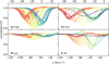 |
Fig. 1 Example CCFs for four pulsating stars as labeled. The color traces the pulsation phase. KN Cen is a long-period, high-amplitude type-I Cepheid. The others are prototypes of their respective pulsating star classes. CCF shape variations follow a characteristic pattern for type-I Cepheids. RR Lyrae stars are hotter and feature shallower CCFs with very large amplitudes and line asymmetry, whereas W Virginis stars can exhibit signatures of shock phenomena at specific phases, including blue-shifted emission features and line splitting. |
2.3 Cross-correlation functions, Gaussian RVs, and uncertainties
All VELOCE RVs were determined using the cross-correlation method (Baranne et al. 1996; Pepe et al. 2002) using correlation templates made to represent a solar-like star of roughly Solar metallicity (G2 mask). The cross-correlation technique reduces the information content of a few thousand spectral lines to a single line profile of extremely high S/N, the so-called cross-correlation function (henceforth, CCF). Example CCFs for two classical Cepheids, RR Lyrae, and W Virginis are shown in Fig. 1. The key benefit of CCFs is that they enable exceptionally precise RV measurements, even from observations with a relatively low S/N. However, the increased RV precision comes at the price of a loss of information that complicates a detailed physical interpretation of CCF profiles.
All VELOCE DR1 RVs are measured as the center position of a Gaussian profile fitted to the CCF. From this Gaussian profile, we also determine the full width at half maximum (FWHM) and the depth (contrast), which we will use in further work. The main advantage of Gaussian RVs is that they afford better precision than other methods commonly applied to Cepheid CCFs, such as CCF barycenters or bi-Gaussian profiles, both of which assign high weight to the lowest point of a CCF profile, where RV constraints are minimal (Anderson 2013, Sect. 2.1.6 and Fig. 2.5). We caution that this choice notably affects the RV peak-to-peak amplitude, which would be largest in case of bi-Gaussian profiles. Moreover, bi-Gaussian profiles are more sensitive to RV curve modulation caused by line shape variations that do not follow the periodicity of the dominant mode, cf. Anderson (2016, Fig. 5). We note that RV uncertainties are estimated differently using Coralie and Hermes as explained in the following.
The RV uncertainties of Coralie data are estimated by the data reduction software based on photon noise statistics and a detailed characterization of the instrument (Bouchy et al. 2001). Figure 2 illustrates that the uncertainties thus derived provide an adequate representation of the statistical precision, that is, the ability to reproduce a measurement within the determined uncertainties under nearly identical conditions. The figure shows the variation of the RV time series around the mean of the sequence for the ~20 days Cepheid RZ Vel near phases of maximal expansion velocity (minimum RV) during 45 min intervals on 22 June 2011 (Coralie07) and again on 5 March 2018 (Coralie14). During each short sequence, virtually no RV variation due to pulsation is expected at pulsation phases of extremal RV, and none is indeed observed. Comparing the dispersion around the mean for each sequence of a given exposure time and the mean RV uncertainty of the same observations reveals excellent agreement; for Coralie07, we find σ(RV −⟨RV⟩) = 0.042 km s−1 for 76 s exposures and σ(RV − ⟨RV⟩) = 0.016 km s−1 for 5 longer 152 s exposures, which compares to the average uncertainties of 0.048 km s−1 and 0.032 km s−1, respectively. For 18 Coralie14 exposures of 90 s each, we find σ(RV −⟨RV⟩) = 0.024 km s−1 and ⟨σRV⟩ = 0.028 km s−1.
RV uncertainties for Hermes observations are based on the covariance matrix of the Gaussian profile fit to the CCF because the instrument has not been characterized to the same RV precision as Coralie. The main shortcoming of this approach is that it does not consider photon noise as the dominant source of RV uncertainty (Bouchy et al. 2001). As a result, RV uncertainties of bright Hermes targets are often overestimated and in reality limited by the short-term stability set by RV drift corrections described in Sect. 2.4. This was previously shown for δ Cephei and Polaris (Anderson et al. 2015; Anderson 2019). RV uncertainties derived from the Gaussian fit covariance matrix tend to be more adequate at lower S/N values (≲30).
Cepheids are complex stars and Gaussian fits to asymmetric CCFs yield biased estimates of the photospheric motion projected onto the line of sight. Yet, these “Gaussian RVs” benefit from very high precision in the differential sense that provide a powerful tool to detect additional variability signals that we collectively refer to as “modulated variability” (Anderson 2014), cf. Sec. 4.3. Hence, studies seeking to interpret Cepheid RVs in an absolute sense, e.g., to determine the Galactic rotation curve, should be warned that several complications limit the accuracy (in an absolute astrometric sense, Lindegren & Dravins 2003) of the measured RVs to the level of a few hundred m s−1. These effects include a) atmospheric velocity gradients and the finite formation height of spectral lines in Cepheids that challenge the notion of “the” RV of the star at any given time at the level of hundreds of m s−1 to km s−1 (e.g., Nardetto et al. 2007; Anderson 2016; Wallerstein et al. 2019), b) spectral line asymmetry not accounted for by Gaussian profiles (Nardetto et al. 2006; Anderson 2013), c) (time-variable) gravitational redshift on the order of a few tens of m s−1 (Dravins et al. 2005; Pasquini et al. 2011), among others. The combination of such effects results in the K-term issue described by Nardetto et al. (2008). We also note that amplitudes determined using other methods for RV determination (including different wavelength ranges) may yield different results, for example, if bi-Gaussian profiles are fitted to the asymmetric CCFs. It is therefore crucial to carefully evaluate whether measurements are sufficiently compatible when combining different datasets, see e.g., Anderson (2019). Further details on related issues have been presented by Anderson (2018b).
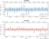 |
Fig. 2 Short-burst (42 and 34 min) RV time series of the 20 days Cepheid RZ Vel near minimum RV collected to test the momentaneous precision of Coralie07 and Coralie14. Both panels show the measured RV minus the mean of the sequence. Shaded areas illustrate the dispersion of the sequences. Average S/N on the 60th echelle order are labeled for reference. Note the improved precision of Coralie14 over Coralie07. Top panel: Coralie07 observations taken on 22 June 2011. Note the change of exposure time (vertical dotted line) that affects both precision and uncertainties estimated by the pipeline. Bottom panel: Coralie14 observations collected on 5 March 2018. |
2.4 RV drift corrections from atmospheric pressure changes
Neither Hermes nor Coralie are pressure-stabilized spectrographs. Atmospheric pressure variations during the course of a night change the diffraction index of the air within the spectrograph, causing a mismatch between the wavelength calibration and the instantaneous wavelength observed at a given pixel location on the detector. Expressed as a shift in velocity space, the displacement of the wavelength solution is usually referred to as an RV drift and measured in m s−1. Atmospheric pressure variations are the leading source of RV drift in modern (temperature-, but not pressure-stabilized) spectrographs and can occur fairly rapidly on timescales of an hour or less.
Coralie RVs collected in OBTH or OBFP modes are corrected for instrumental drift using a simultaneous wavelength reference that is interlaced between the science orders. However, RVs measured using Coralie OBJO and Hermes OBJ_HRF observations are subject to instrumental drift that we aimed to mitigate using a physical model of the RV drift due to ambient pressure changes.
The physical model for atmospheric drift correction was developed by Anderson (2013, Ch. 2.1.5) and predicts the following RV drift correction for a change of atmospheric pressure, ΔP, in mbar:
![Mathematical equation: $\[\Delta v(\Delta P) \approx 2.7 \times 10^{-7} \cdot \Delta P \cdot c \approx 81 \cdot \Delta P\left[\mathrm{~m} \mathrm{~s}^{-1} \mathrm{~mbar}^{-1}\right],\]$](/articles/aa/full_html/2024/06/aa48400-23/aa48400-23-eq1.png) (1)
(1)
where c is the speed of light in m s−1.
We adopted this model to correct RV drifts of 3359 Coralie observations collected in OBJO mode as well as of all Hermes (OBJ_HRF) observations. Figure 3 shows a comparison of our RV drift model to 4667 Coralie observations collected in OBTH mode. The model adequately represents RV drifts, and we found a small global offset of ~5 m s−1 and a 10% larger RV drift estimate based on the simultaneous reference compared to the pressure model. Part of the scatter in this relation is due to the rather coarse 0.1 mbar resolution of ambient pressure in the data headers, as well as differences between the pressure measured by the weather station and the air pressure inside the instrument. Of course, the best results are achieved when this model is used in conjunction with intra-night wavelength recalibrations scheduled when atmospheric pressure variations exceed ±0.5 mbar to avoid large corrections. Based on this comparison, we estimate a systematic uncertainty of approximately 10–15 m s−1 for this correction and conservatively added 15 ms−1 in quadrature to the reported RV uncertainties for Coralie OBJO and Hermes observations. Further improvements to this models would be feasible by considering the impact of the altitude of the observatory on the model as well as other instrument parameters, such as grating or CCD temperatures. However, the first-order approximation presented here is sufficient for our purposes.
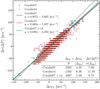 |
Fig. 3 RV drift corrections determined from pressure variations (Eq. (1)) against the corrections determined via simultaneous drift corrections based on interlaced ThAr spectra. The discretization of the results is due to the single-decimal precision with which the atmospheric pressure is recorded in the FITS headers. The black dotted line shows the equality Δυ(ΔP) = ΔυTh, whereas the blue, red, and green lines are the best linear fits to the Coralie07, Coralie14, and combined Coralie distributions, as quantified in the legend. |
2.5 RV standard stars
We tracked the long-term stability and absolute RV scale of Hermes and Coralie using IAU RV standard stars (Udry et al. 1999a,b). In particular, we investigated whether the installations of fibers with octagonal cross-sections (2014 for Coralie, 2018 for Hermes) impacted RV zero-points and precision. Tables 1 and 2 list the spectral types, CCF full FWHM, and RVs determined before and after the two upgrades, alongside the differences and a mean offset. For Hermes, we note a factor of 2 improvement in the dispersion of standard star RVs thanks to the upgrade (from 0.038 to 0.019 km s−1), as well as a systematic increase in RV by 0.075 ± 0.007 km s−1. For Coralie, the weighted average of the zero-point offsets is −0.0267 ± 0.0005 km s−1. A more detailed inspection of the Coralie zero-point would need to account for differences in FWHM. However, this is out of scope here and will be presented elsewhere (Segransan et al., in prep.). Neither of the zero-point shifts have been applied in VELOCE DR1 because sufficient standard star information was not available at the time when the Cepheid light curves were fitted. Future data releases will be corrected for these zero-point offsets. We note that the typical root mean square of Cepheid RV curve residuals typically exceeds 50, if not 80, m s−1 due to stellar effects (Sect. 4.3), so that the zero-point changes do not challenge any of the conclusions presented here. However, studies targeting very detailed investigations of modulated variability should certainly account for these zero-point shifts.
Hermes RV standard stars.
Coralie RV standard stars.
2.6 Sample selection and observational strategy
Observations for the VELOCE project have been collected using Coralie and Hermes since November 2010. From 2010 to mid-2019, access to the Euler and Mercator telescopes was typically available during 10 (Hermes) and 14–15 night (Coralie) observing runs. Data obtained during that time frame hence tends to “clump” within windows of about two weeks, with some exceptions made possible via time exchanges with other groups. On both telescopes, data were typically collected during two to three observing runs per year. Subsequent observing runs were spaced by at least two weeks, and up to several months apart. This mode of access to both telescopes was well suited for achieving good phase coverage for Cepheids with P ≲ 11–15 days. For longer-period Cepheids, efforts were made to complete phase coverage via time exchanges and by considering pulsation phases accessible for each star in every given observing run. Some observing runs were also specifically timed such as to coincide with pulsation phases of interest for specific very long-period Cepheids. This close monitoring of accessible pulsation phases for all sources during all observing runs made it possible to obtain very good phase sampling over relatively short periods of time so that orbital motion and other modulations could be well separated from pulsational variability and uncertainties related to the pulsation ephemerides.
Observations for VELOCE were involuntarily interrupted between the end May 2019 and March 2021, first due to changes in telescope operations and funding, and second due to uncertainties of the lead author’s postdoctoral career path during the COVID-19 pandemic. Thankfully, time exchanges and the good will of observers, as well as KU Leuven and Mercator staff, made it possible to obtain additional observations of δ Cephei in 2020, with crucial importance for constraining its highly eccentric orbit by probing times near the most extreme orbital velocities (cf. Paper II).
In March 2021, VELOCE observations resumed on both telescopes thanks to funding provided by the European Research Council. Observations collected since March 2021 follow a very different temporal sampling, which seeks to provide a more even monitoring across the year. New observations on Euler in particular can target very specific pulsation and orbital phases, and were used to fill in gaps in phase coverage and to extend baselines for many stars to improve sensitivity to orbital motion.
The selection function of VELOCE as a survey is not well defined, since VELOCE was not initially conceived as a long-term project. The sample of stars was regularly modified for a variety of reasons and science interests, which notably included (1) to densely sample pulsation periods most relevant to tracing the Hertzsprung (1926) progression spectroscopically; (2) long-period Cepheids with high-quality parallax measured using the Hubble Space Telescope (HST) or Gaia as well as Cepheids with photometric observations from HST (Anderson et al. 2016a; Riess et al. 2018b,a, 2021) owing to their importance for the extragalactic distance scale; (3) Cepheids observed with longbaseline optical interferometry (e.g., Breitfelder et al. 2016; Anderson et al. 2016b; Gallenne et al. 2019), e.g., to calibrate Baade-Wesselink projection factors; (4) spectroscopic binary Cepheids, notably ones fainter than ~8–9th magnitude, with brighter Cepheids included as fillers and to achieve orbital solutions; (5) known or suspected spectroscopic binaries as well as new binary candidates discovered by the ongoing program; (6) very bright Cepheids, such as η Aql, ℓ Car, or δ Cep, to obtain RV curves and spectral time series of exceptional quality, e.g., to study line shape variability and atmospheric effects (e.g., Anderson 2016); (7) possible signatures of shock-related phenomena; (8) monitoring Cepheids whose RV curves exhibit signatures of additional signals, such as long-term amplitude variations or cycle-to-cycle fluctuations (Anderson 2014); (9) Cepheids in the vicinity of open clusters (Anderson et al. 2013; Cruz Reyes & Anderson 2023); (10) spectroscopic follow-up of less well studied Cepheid candidates from the All Sky Automated Survey (ASAS; Pojmanski 2002, 2003; Pojmanski & Maciejewski 2004, 2005; Pojmanski et al. 2005) and other ground-based surveys, including objects located away from the Galactic plane as filler objects when no other targets were observable; (11) a few type-II Cepheids and RR Lyrae stars observed when no classical Cepheids were observable (12) RV standard stars, notably on Hermes.
A large number of Cepheid candidates from photometric surveys were found to be non-Cepheids based on their spectral properties, notably the absence of a clear CCF peak, multiple peaks, or absence of line shape variability, cf. Anderson (2013). Limited information concerning these targets is provided in Appendix B.
We aimed to collect at least three, better four or more, epochs of reasonably well sampled RV phase curves. Depending on the observational progress, priorities and strategies were adapted to ensure that interesting phenomena could be followed up. The focus throughout was to obtain measurements with uncertainties <50 m s−1 per observation. Most observations targeted S/Ns of at least 20 (more commonly 25–30) per pixel near 5500 Å. For fainter stars, the target S/N was lowered to ~10 due to the limited collecting area, producing satisfactory results notably for detecting orbital motion given the somewhat larger RV uncertainties reaching 100 m s−1. Higher target S/Ns were adopted for bright Cepheids of interest. For Cepheids visible to the naked eye, typical S/Ns exceed ~100 per pixel. As a result, a subset of observations is viable for more detailed spectroscopic analysis, although the S/N of the majority of observations may be too low for this purpose.
3 A high-precision catalog of Cepheid RVs
VELOCE DR1 delivers 19 386 RV measurements of 258 bona fide MW classical Cepheids and 164 stars that are not classical Cepheids. The targets are distributed across both hemispheres and clearly trace the Galactic disk, cf. Fig. 4. The dominant uncertainty on the RV measurements is photon noise, so that there exists a fairly clean correlation between the best RV uncertainties and the magnitude of the source, which, however, can be altered by differences in S/N and astrophysi-cal effects. The dependence of the mean RV uncertainty vs. magnitude is illustrated in Fig. 5. We note that the different estimation of RV uncertainties by the Coralie and Hermes pipelines lead to overestimated Hermes uncertainties, especially at bright magnitudes. An uniquely extreme example of this is the bright 7 days Cepheid X Sgr (not shown), for which Hermes and Coralie uncertainties can differ by two orders of magnitude. However, this particular issue is limited to X Sgr, where significant line deformations (Mathias et al. 2006; Anderson 2013) complicate the interpretation of RVs and their uncertainties.
RV time series of stars that are not classical Cepheids are provided “as-is”, meaning that the output of the reduction pipelines was not vetted. For example, multi-lined binaries will generally result in a single RV measurement, although it is unclear which component is being measured. The reduced spectra and CCFs of non-Cepheids are available upon request from the author.
For 253 single-mode classical Cepheids in our sample (henceforth: the Cepheid sample), we determined the pulsation-averaged velocity υγ, best-fit Fourier series models, and pulsation ephemerides. Figure 6 shows the distribution of Cepheid pulsation periods in VELOCE and highlights the sample used to assess zero-point differences with literature Cepheid RVs, whereas Fig. 7 shows the distribution of the number of observations per target (~50). Table A.1 lists our preferred identifiers, coordinates at epoch J2000, Gaia DR3 source identifiers, the intensity-averaged Gaia G-band and average GBp – GRp color, pulsation mode, a binary flag (SB1 for single-lined spectroscopic binary), the number of observations available, Nobs, the number of Fourier harmonics used to fit the star, NFS, pulsation period Ppuls, and the reference epoch E used for the fit. The binary flag indicates whether we consider a given star to exhibit orbital motion based on the VELOCE data set alone, since this affects the modeling choice for the Fourier series model. Spectroscopic binaries are investigated in detail in Paper II, including also literature data. Table A.1 also contains the names of bona fide Cepheids for which we report RV time series without Fourier modeling, e.g., due to lack of data or particularly complex signals.
Table B.1 provides summary information for 164 non-classical Cepheids, including 4 RR Lyrae stars, 12 type-II Cepheids, 33 (candidate) double- or triple-lined binaries.
Compared to Gaia DR3, VELOCE contains ~3000 more individual RV measurements of classical Cepheids (18 225), albeit of much fewer stars (253 vs. 731). VELOCE data thus generally sample RV curves more closely and over longer temporal baselines, similar to Gaia’s end-of-mission baseline. A detailed comparison of VELOCE to Gaia RVs is provided in Sect. 5.4. Figure 8 illustrates the completeness of VELOCE relative to 1098 Gaia DR3 MW Cepheids (from the Specific Objects Studies table gaiadr3.vari_cepheids) with P > 0.9day and G < 13.3 mag. The blue histograms show the fractions of Cepheids observed by VELOCE over the Gaia sample as a function of magnitude (left) and Ppuls (right). Red histograms show the fraction of Gaia DR3 Cepheids with RV time series (559 Cepheids from table gaiadr3.vari_epoch_radial_velocity) to the same photometric sample. Unsurprisingly given the small telescope diameter, the completeness of VELOCE is a strong function of magnitude, and only few stars fainter than 12th magnitude were observed.
VELOCE data are made available in FITS format via Zenodo alongside supporting python code to facilitate data access. Appendix C provides details on the data structures containing VELOCE data and fit results. All data tables presented in this article will additionally be made available in machine-readable form via the Centre de Données de Strasbourg.
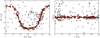 |
Fig. 4 Sky coverage of VELOCE targets in sky coordinates (left) and Galactic coordinates (right). Bona fide Cepheids are shown as red filled circles, stars that are not classical Cepheids are shown as open circles. |
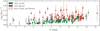 |
Fig. 5 Mean per epoch RV uncertainty of bona fide Cepheids with at least 9 observations as a function of the mean Gaia DR3 G-band magnitude, cf. Table A.1. Coralie uncertainties (green points) are estimated differently from Hermes uncertainties, cf. Sect. 2.3, and are limited by photon noise. Hermes uncertainties (red points) are overestimated for G ≲ 10 mag. The brightest star, Polaris, is missing due to a lack of Gaia photometry; the faintest target is GL Cyg. X Sgr is excluded from the plot due to significant line shape distortions (Mathias et al. 2006; Anderson 2013) that complicate uncertainty estimation. |
3.1 Fourier series model fitting
We modeled the observed RV time series, υr(t), of single-mode bona fide Cepheids using Fourier series with n harmonics as
![Mathematical equation: $\[v_r(t)=v_\gamma+\sum_{n=1,2,3, \ldots} a_n \cos (2 n \pi \phi)+b_n \sin (2 n \pi \phi),\]$](/articles/aa/full_html/2024/06/aa48400-23/aa48400-23-eq2.png) (2)
(2)
where υγ denotes the pulsation averaged velocity, t the midpoint of the shutter opening time in barycentric Julian Date, ϕ = (t – E)/Ppuls the pulsation phase, Ppuls the pulsation period, and E the reference epoch. Secular period changes due to stellar evolution are typically irrelevant over the timescale of the VELOCE baseline, whereas irregular or periodic period changes appear to various degrees, but cannot be adequately modeled using the available data. However, the longer baselines covered by our template fitting analysis (Sect. 5.1) requires solving for phase shifts over time, which we use to measure period changes in Sect. 5.3. Following Anderson (2016), E is defined such that ϕ = 0 coincides with υγ on the steeper, descending branch of the RV curve close to the mean observation date. This definition identifies the phase of minimum radius, which has several advantages over maximum light: a) it is most precisely measurable thanks to the steepest gradient with time; b) ϕ = 0 corresponds to the same state of the pulsation regardless of period; c) it does not require contemporaneous photometry. For reference, ϕ = 0 typically occurs slightly before (δϕ ~ 0.1–0.2) maximum light. The best-fit parameters are obtained by non-linear least squares.
Cepheid RV curves differ in complexity, depending both on pulsation mode and period, and every Cepheid in VELOCE has been observed a different number of times. The most appropriate number of harmonics, NFS, of the Fourier series fit must therefore consider both RV curve morphology and Nobs. We adopted a sequential brute-force approach to determining the optimal model and Ppuls simultaneously. First, we fitted each RV time series using 1 ≤ n ≤ min[20, (Nobs − l)/2] Fourier harmonics. Since the best-fit Ppuls can depend on NFS, we performed phase dispersion minimization for every order (NFS) separately within typically 0.5% of the literature pulsation period used as a starting value. Some short-period (overtone) Cepheids exhibit rather fast period fluctuations and thus required slightly larger flexibility for finding a best-fit Ppuls. For all but a few Cepheids, this procedure very effectively minimized phase scatter. The epoch E was then computed to match ϕ = 0 at minimum radius. Uncertainties on Ppuls and E were obtained by Monte Carlo simulations, and we assign systematic uncertainties on Ppuls and E as half the difference between the values of Ppuls of the next higher and lower harmonics. Both uncertainties contribute roughly equally to the total uncertainty and are reported separately in the data files, whereas their squared sum is used in the text.
We performed sequential model comparison using an F-test and the Bayesian Information Criterion (BIC) to select the optimal model. For the F-test, we adopt p = 0.05 as the significance level for comparing models with n vs. n + 1 harmonics. Analogously for the BIC, greater model complexity is considered acceptable if BIC decreases with increasing model complexity. We conservatively adopted as the optimal n the number of harmonics above which either the F-test or the BIC criterion indicated spurious improvement. Figure 9 illustrates this sequential model comparison. The final selected models were also inspected visually. Two possible exceptions to these rules were allowed: a) for seven Cepheids (AB Cam, CH Cas, KX Cyg, RY Sco, U Sgr, WW Mon, Z Lac), we adopted lower n after visual inspection; b) we implemented an automated rule that allowed us to skip ahead to the next higher harmonic (n + 1) if n < 10 and more than one of the following more complex models (e.g., n + 2 and n + 3) satisfied both statistical tests. Figure 10 illustrates the resulting distribution of NFS relative to the data available.
SB1 Cepheids exhibit temporal variations of the pulsation average velocity, so that υγ = υγ(t) in Eq. (2). These variations occur on timescales longer than Ppuls and are discussed systematically in Paper II. Following visual inspection of Fourier series residuals, we identify Cepheids exhibiting orbital motion in the VELOCE time series data in Table A.1.
We caution that time-variable line shape distortions can lead to spurious trends in Fourier series residuals that could be mistaken for evidence of orbital motion depending on sampling (Anderson 2014, 2016), and we considered this effect in setting the SB1 flag. Furthermore, some Cepheids exhibit large phase dispersion due to rapidly (possibly stochastically) varying Ppuls, e.g., SZ Tau, and the long-period Cepheids SV Vul and S Vul. Period “jitter” reported in Cepheids (e.g., V1154 Cyg, cf. Derekas et al. 2017) introduces a scatter floor in the Fourier fit residuals. Expressed in root mean square, the minimum residual scatter can be as low as ~60 m s−1, although values around 100–120 m s−1 are more common and can reach up to several hundreds of m s−1 (Sect. 4.3). In such cases, a simple mono-periodic Fourier series cannot provide an adequate fit to the data due to the additional signals.
To determine the pulsation periods of Cepheids exhibiting time-variable υγ(t) (binaries or not), we represented the variable pulsation average velocity in Eq. (2) by a polynomial with coefficients ci:
![Mathematical equation: $\[v_\gamma=v_\gamma(t)=v_{\gamma, E}+\sum_{i=1, \ldots} c_i \cdot(t-E)^i.\]$](/articles/aa/full_html/2024/06/aa48400-23/aa48400-23-eq7.png) (3)
(3)
The polynomial allows us to represent modulated variability of any origin (aside from variable Ppuls) while determining Ppuls and E, and higher degree i implies more complex and/or shorter-timescale modulations. This was particularly useful for dealing with high-amplitude orbital motion, especially when the orbital signal was incompletely sampled. Given the long baselines of VELOCE, all polynomials trace timescales much longer than Ppuls. The degree of any polynomials plotted are listed alongside the Fourier series coefficients in Table A.2. We caution that the constant term, υγ,E, is defined at the epoch E when such polynomials are used, and thus, it should not be used to represent the center-of-mass velocity of the star. Further discussion of the polynomial parameters and of SB1 Cepheids is presented in Paper II.
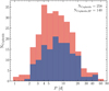 |
Fig. 6 Distribution of pulsation periods of Cepheids in VELOCE. The red histograms shows all classical Cepheids, while the blue histogram shows the stars used to determine instrumental zero-points, cf. Sects. 5.2 and 5.4. |
 |
Fig. 7 Distribution of the number of observations per Cepheid. The red histogram shows the available number of observations (Nobs) of all Cepheids in VELOCE. The blue histogram shows the number of measurements used to fit Cepheid RV curves (Nobs,fitted). The bin edges are identical for both histograms and logarithmically spaced. The first 8 bins of the red histogram are shown individually to improve readability; a threshold of at least 9 observations was used to fit pulsational models (Sect. 3.3.1). Differences between the blue and red histograms at Nobs > 8 arise due to data selection for model fitting (e.g., in the case of binaries, Sect. 3.3) or additional signals preventing a reasonable fit (Sect. 4.3). The legend summarizes the median and total number of VELOCE observations per group. |
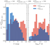 |
Fig. 8 Distributions of the number ratios of Cepheids in VELOCE to those in Gaia as a function of magnitude (left) and Ppuls (right). The comparison is limited to 245 VELOCE Cepheids for which G-band magnitudes are available and to |
![Mathematical equation: $\[N_{\text {GaiaDR3,phot }}^{\text {Cep }}=1098\]$](/articles/aa/full_html/2024/06/aa48400-23/aa48400-23-eq3.png)
![Mathematical equation: $\[N_{\mathrm{GaiaDR3,RV}}^{\mathrm{Cep}}=559\]$](/articles/aa/full_html/2024/06/aa48400-23/aa48400-23-eq4.png)
![Mathematical equation: $\[N_{\text {VELOCE }}^{\mathrm{Cep}} / N_{\mathrm{GaiaDR} 3, \text { phot }}^{\mathrm{Cep}}\]$](/articles/aa/full_html/2024/06/aa48400-23/aa48400-23-eq5.png)
![Mathematical equation: $\[N_{\text {GaiaDR3,RV }}^{\mathrm{Cep}} / N_{\text {GaiaDR3,phot }}^{\mathrm{Cep}}\]$](/articles/aa/full_html/2024/06/aa48400-23/aa48400-23-eq6.png)
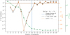 |
Fig. 9 Illustration of the automated model selection procedure. Up to twenty harmonics were computed in a brute force approach, depending on data availability. The statistical significance of increasing the model’s complexity was assessed using both F-test (p < 0.05) and BIC (ΔBIC < 0) criteria. Violations of these criteria were accepted if the two subsequent, more complex, models both indicated significant fit improvements. The improvement χ2/NDOF of the fit is shown in green. |
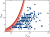 |
Fig. 10 Number of Fourier series harmonics (NFS) used vs. number of observations available (Nobs). The black dash-dotted line shows the maximum number of harmonics that can be fitted for a given number of observations, Nobs = 2 • NFS + 1. The red dotted lines and shaded area show increasing numbers of degrees of freedom (up to ND0F = 10). |
3.2 Fourier amplitude ratios and phase differences
Fourier amplitude ratios and differences were computed using the best-fit Fourier series coefficients, ai and bi (cf. Eq. (2)), in order to easily visualize the Hertzsprung progression in Sec. 4.1 (Simon & Lee 1981). The amplitude and phase of the ith harmonic are defined as ![Mathematical equation: $\[A_i=\sqrt{a_i^2+b_i^2}\]$](/articles/aa/full_html/2024/06/aa48400-23/aa48400-23-eq8.png) and tan ϕi = − bi/ai. Amplitude ratios among harmonics are defined as Ri1 = Ai/A1, and phase differences as ϕi1 = ϕi − i • ϕ1. Uncertainties on Ai and ϕi are determined using the covariance matrix of the fit and propagated to compute uncertainties for Ri1 and ϕi1.
and tan ϕi = − bi/ai. Amplitude ratios among harmonics are defined as Ri1 = Ai/A1, and phase differences as ϕi1 = ϕi − i • ϕ1. Uncertainties on Ai and ϕi are determined using the covariance matrix of the fit and propagated to compute uncertainties for Ri1 and ϕi1.
3.3 Stars exempted from detailed Fourier modeling
This data release contains 1070 observations of 39 Cepheids whose variability could not be satisfactorily modeled using a mono-periodic Fourier series due to insufficient sampling, multi-periodicity, or additional signals. We here publish the time series RV measurements for these stars without detailed Fourier modeling and include them separately in Table A.1.
An exception is the overtone Cepheid SU Cyg (Imbert 1984, Paper II), whose high-amplitude and short-period orbital motion prevented an adequate fit using the polynomial Fourier series model using only VELOCE data. Similarly, insufficient phase coverage and few measurements prevented a good Fourier series fit for ER Aur and SU Cas.
The RV time series of VX Cyg featured a noticeable gap of about 0.2 in phase along the slowly rising RV branch, which makes up about 0.7 in phase. During this phase, stars of this period exhibit linearly increasing RV. To obtain a clean Fourier series fit, we therefore linearly interpolated between the observed points along the rising branch and added the interpolated points with conservative 0.2 km s−1 uncertainties. The interpolated points are included in the data set for VX Cyg and clearly marked in column ‘SOURCE’ of the data tables, cf. Table C.6.
3.3.1 Cepheids with insufficient Nobs for Fourier modeling
Twenty-eight Cepheids featured an insufficient number of observations to adequately reproduce their variability curves: AP Cas, ASAS J074902−1906.8, ASAS J075345−3658.2, ASAS J082710−3825.9, ASAS J084304−5117.9, ASAS J094827−5801.1, ASAS J103052−5903.7, ASAS J115701−6218.7, ASAS J122511−6120.9, ASAS J181215−2029.1, ASAS J183347−0448.6, ASAS J183652−0907.1, ASAS J191351+0251.3, ASAS J192310+1351.4, BR Vul, CG Cas, DW Cas, EV Aql, GM Cas, GSC 03996−00312, TV CMa, U Aql, V0335 Aur, V0458 Sct, V0493 Aql, V0600 Aql, V1954 Sgr, and X Sct. While no classification was assigned for ASAS J082710−3825.9 in Gaia DR3, we find an RV difference of ~16 km s−1 among two measurements separated by 3 nights (Ppuls = 9.3 days), which is easily compatible with the typical peak-to-peak amplitudes of Cepheids around this period. Moreover, the star’s CCFs exhibit the typical shape variation expected from a classical Cepheid.
3.3.2 Cepheids exhibiting non-stationary variability
Two peculiar amplitude-modulating Cepheids could not satisfactorily be modeled using a stationary Fourier series: the well-known Blazhko Cepheid V0473 Lyr (Burki & Mayor 1980; Molnár & Szabados 2014) and the spectroscopic binary Cepheid ASAS J103158–5814.7 whose Blazhko modulations and orbital motion are reported here for the first time. RS Pup’s strong cycle-to-cycle variations and period fluctuations similarly prevented an adequate fit. Additional information on such phenomena is presented in Sec. 4.3.
3.3.3 Double-mode (beat) Cepheids
Five double-mode (beat) Cepheids were observed: MS Mus, TU Cas, V1048 Cen, V1210 Cen, and Y Car. The RV time series collected are published as part of this data release. However, they were not modeled due to the added complexity of determining two pulsation periods based on RV data and the generally short pulsation timescales of double-mode Cepheids.
3.3.4 RR Lyrae stars and type-II Cepheids
VELOCE targets classical Cepheid variables. However, four RR Lyrae stars and twelve type-II Cepheids were observed as backup targets at times when an insufficient number of Cepheids were visible during a particular observing run, or, in the case of the prototype RR Lyrae, to obtain a base for comparison with classical Cepheid variability of CCFs. We did not model these stars because the number of observations available for these stars was generally lower and because type-II Cepheid RV curves exhibit more scatter than those of classical Cepheids. Further information is presented in Appendix B.
Table B.1 lists these stars and the number of RV measurements presented here alongside additional information. The RV time series for these stars are included without detailed Fourier modeling and were derived using the same procedure as the one applied above for classical Cepheids. However, we note that the G2 mask is not applicable to the hottest phases of RR Lyrae stars, resulting in no correlation peaks (hence, no RVs) along the fast-changing descending RV branch (cf. Fig. 1). Type-II Cepheids, such as W Vir, exhibit blue-shifted emission features indicative of shock that may further influence RV measurements (cf. Fig. 1).
4 New insights from precision velocities
The combination of a large sample of Cepheids observed with unprecedented precision over a decade-long baseline provides interesting new insights into the astrophysics of Cepheids. In the following, we highlight a) the Hertzsprung progression observed from RV data in unprecedented detail (Sec. 4.1), b) the discovery of a secondary bump in Cepheid RV curves that also follows the Hertzsprung progression (Sec. 4.2), c) the ubiquity of modulated variability features, such as long-term modulations and cycle-to-cycle variations (Sec. 4.3), and d) a puzzling dichotomy among the linear radius variations exhibited by Cepheids (Sect. 4.4).
4.1 The Hertzsprung progression
The Hertzsprung progression (Hertzsprung 1926, HP) refers to an apparently continuous change in the light curve shapes of Cepheids pulsating in the fundamental mode as a function of their pulsation period. It is one of the most noticeable features of Cepheids light and RV curves and provides insights into the physics of stellar pulsations. Additionally, the HP can be used to illustrate the similarity of extragalactic and nearby Cepheids to underline their physical similarity (Riess et al. 2022). Although Hertzsprung (1926) already considered Fourier components in relation to the HP, the visualization of the HP using ratios of Fourier parameters has been common since Simon & Lee (1981).
Cepheid RV curves are known to also exhibit the HP, although the sampling in period had been rather limited until recently. Prior to Gaia DR3, the most detailed investigations of the RV HP were presented by Kovacs et al. (1990, based on 57 Cepheids of mostly short periods), Gorynya (1998, using phase shifts and asymmetries rather than Fourier decomposition), and Anderson et al. (2016a, including additional long-periods), who remarked a group of (then: four) long-period Cepheids with particularly low RV amplitudes further discussed in Sec. 4.4.
The VELOCE HP is illustrated in Fig. 11, which shows the peak-to-peak RV amplitude, Ap2p, the amplitude of the first harmonic, A1, as well as the ratio of the ith harmonic’s amplitude to the first harmonic’s amplitude (Ri1) and analogous for the Fourier phase differences (ϕi1) of several higher-order harmonics (2 ≤ i ≤ 7) to the first harmonic. Features known from photometric illustrations of the HP are accurately recovered, notably including the “dip” in Ap2p near 10 days (Klagyivik & Szabados 2009), the sharp divide between overtone and fundamental mode pulsators in R21, the flattening of ϕ21 at longer Ppuls. Since the number of harmonics can differ among VELOCE stars, the number of objects decreases for higher harmonics (cf. Eq. (2)).
The color coding according to NFS in Fig. 11 shows that stars that have been modeled using higher NFS exhibit extremely clean trends, in particular among the phase ratios. Outliers tend to have a smaller number of harmonics, indicating that there were too few observations available to capture the full complexity of the RV curve. A particularly interesting case is that of the 17-day Cepheid Y Oph, which was modeled with a very low number of harmonics (NFS = 4) despite a large number of available observations, and which exhibits Fourier parameters that appear as a long-period extension from overtone Cepheids, especially among A1 and R21. This is curious given that the longest-period overtone Cepheid in the MW has a period of only 8.8 days (Baranowski et al. 2009).
Further interesting features in Fig. 11 are the increased dispersion among higher-order amplitude ratios at log P ≳ 1.15, as well as the increased dispersion in the higher-order phase ratios that is restricted to the period range around 0.95 ≲ log P≲ 1.25 (9–18 days). Additional visualization of these results is provided in Appendix A.1.
Figure 12 illustrates the HP using all fitted Fourier series models. The vertical axes show RV, with each star being offset according to log P as marked on the right. The left panel shows the full period range, with the left column being populated by low-amplitude Cepheids, most of which pulsate in the first overtone, as well as Y Oph and YZ Car, two long-period Cepheids featuring atypically low RV amplitudes. The right column of the left panel shows fundamental mode Cepheids and very clearly exhibits the “bump” feature that appears near phase 0.75 for a Cepheid with log P ≈ 0.75 and moves to lower phase with increasing period until it disappears at log P ≳ 1.55. The bump is most noticeable when it appears on the descending part of the RV curve, that is, near minimum radius, and it can very significantly stretch the descending branch and render it much less steep. While the RV HP is very clearly observed, we note that some Cepheids clearly do not exhibit RV curves representative of other Cepheids at similar log P.
The right panel of Fig. 12 provides a close-up view of Cepheids in the period range where this is most noticeable, around 9–18 days, and we note that this period range is also where the higher-order Fourier phase ratios exhibited excess scatter.
4.2 A second bump in the Hertzsprung progression
Figure 12 (right panel, right column) shows that 31 of the 61 (50%) Cepheids in the HP period range exhibit an additional bump feature, whereas 30 Cepheids exhibit the expected single bump on the descending branch. Figure 13 shows a close-up view of XX Car to illustrate that the double bump is not caused by ringing or poor sampling. This double bump feature has not previously been reported in the literature6 in Cepheid light or RV curves and could be identified here thanks to the precision of VELOCE data. One of the targets that exhibit this feature (albeit not very strongly) is the 3rd magnitude star β Dor, which fortuitously lies within the TESS Southern Continuous Viewing Zone and therefore benefits from a particularly long-baseline high-precision photometry. Inspection of the light curve presented in Plachy et al. (2021) reveals a clear photometric double bump, although this feature was not recognized as such at the time, likely due to the lack of comparison stars exhibiting similar features. Comparison with TESS light curves for additional Cepheids will be particularly useful to shed further light on these potentially useful features of stellar pulsations. Given that the well-known bump is explained by a resonance among the fundamental mode and second overtone (Kovacs et al. 1990; Antonello & Morelli 1996), it would seem likely that the double bump feature is also caused by overtone resonances, which may provide important new insights into the structure and evolution of Cepheids.
As Fig. 14 shows, double bump Cepheids have nearly constant ϕ41 across a broad range of R21 and do not appear to follow the bulk of other Cepheids in this diagram. Additionally, double bump Cepheids follow a different trend in the ϕ41 − ϕ31 vs. R21 diagram.
4.3 Long-term modulations and cycle-to-cycle variations
Cepheid RV curves have been shown to exhibit signals that cannot be explained by the standard Fourier series fitting approach with a fixed period7. In an early result based on VELOCE data, Anderson (2014) showed the existence of at least two different categories: long-term amplitude modulations of short-period (likely overtone) Cepheids, such as V0335 Pup and QZ Nor, and cycle-to-cycle fluctuations affecting both the RV curve shape and periods of long-period Cepheids such as ℓ Car and RS Pup (cf. also Anderson 2018b). A growing body of literature has since pointed out the generally less stable behavior of overtone Cepheids, as well as the existence of additional pulsation modes, many of which are hiding underneath unstable main modes of pulsations (e.g., Derekas et al. 2012, 2017; Evans et al. 2015b; Poretti et al. 2015; Soszyński et al. 2015; Smolec & Śniegowska 2016; Smolec 2017; Süveges & Anderson 2018b,a; Rathour et al. 2021; Csörnyei et al. 2022; Smolec et al. 2023). Cycle-to-cycle variations in long-period Cepheids probe the interplay of convection with pulsations (Anderson 2016; Anderson et al. 2016b) and appear to be mostly stochastic. By contrast, long-timescale modulations of overtone Cepheids may be repeating (Anderson 2018b), or even periodic, although the physical origin is less clear. Additionally, V0473 Lyr (Burki & Mayor 1980; Molnár et al. 2017) exhibits large periodic amplitude modulations reminiscent of the Blazhko-effect (Blažko 1907) seen in RR Lyrae stars, whereas Polaris exhibits multi-periodic line profile variations (Hatzes & Cochran 2000; Anderson 2019; Torres 2023). Moskalik & Kołaczkowski (2009) further reported Blazhko-like modulation in LMC double-mode Cepheids.
VELOCE data provide a powerful complement to space-based photometry for studying modulated variability thanks to high zero-point stability. While space-based photometry benefits from high precision and the ability to collect time series uninterrupted by the diurnal cycle, temporal baselines longer than a few months to a year are difficult to achieve from space for a large number of Cepheids. Unfortunately, only a single Cepheid (V1154 Cyg) was observed by Kepler (Derekas et al. 2017), and the temporal baseline of TESS (Ricker et al. 2015) is rather short outside of the continuous viewing zones. Nevertheless, TESS observations of Cepheids (Plachy et al. 2021) probe up to several pulsation cycles extremely densely and without interruption. A systematic comparison between the variability signals observed by TESS and VELOCE is therefore of interest.
For bright stars such as ℓ Car, the pulsational RV amplitude of order 35 km s−1 is 7000–10000 times larger than the typical 3–5 m s−1 RV uncertainty achievable using Coralie. For comparison, a typical V-band amplitude of a similar Cepheid would be of order 1 mag, requiring a stable photometric uncertainty of 0.14 mmag over the course of two months to trace two full pulsation cycles in similar detail. Even considerably poorer RV precision of 50–70 m s−1 still corresponds to an S/N of 500–700. Hence, VELOCE is highly sensitive to interesting additional signals that may help to further improve the understanding of these stars.
We find that a typical RV uncertainty of 40–50 m s−1 will provide basic sensitivity to such additional signals, although 10–20 m s−1 will render them much more obvious. Figure 15 illustrates this by plotting the reduced χ2/NDOF of the model against the median RV uncertainty, where N<sc>dof</sc> is the number of degrees of freedom of the fit. Most Cepheids with typical uncertainties better than 20 m s−1 yield χ2/NDOF of several tens to hundreds or even thousands. Of course, inadequate temporal sampling or model complexity will contribute to higher χ2 and contributes to the scatter seen in Fig. 15. However, the clear trend to higher reduced χ2 for better measurements is not explained by missing data and instead confirms the result by Süveges & Anderson (2018a) based on OGLE photometry that modulated variability becomes a ubiquitous feature among LMC Cepheids given sufficiently precise measurements. Overall, we find 19 Cepheids with χ2/NDOF > 100, of which 16 have a median error <40 m s−1. Interestingly, some of the longest-period Cepheids in the sample, GS Lup, SV Vul, and S Vul also fall into this group despite median errors of 44, 44, and 77 m s−1, respectively. This indicates that very long-period Cepheids are particularly unstable and exhibit ubiquitous cycle-to-cycle variations similar to the ones reported in ℓ Car and RS Pup (Anderson 2014, 2016; Anderson et al. 2016b).
Table 3 lists Cepheids exhibiting (clear or tentative) modulated variability phenomena (e.g., not orbital motion) grouped according to different types of phenomena named ad hoc according to the first object where this type of variability was seen during the course of the collection of the VELOCE data set. The sheer number of stars exhibiting these phenomena demonstrates the power of high-precision RVs to provide significant new information in the study of Cepheids, while the diversity of phenomena implies that more than one physical effect is at play. We will specifically study this “Modulation Zoo” in future work, the first of which will present the detection of non-radial modes using spectroscopic observations (Netzel et al. 2024).
A few cases merit specific mention. MY Pup exhibits V0335 Pup-like amplitude modulations and is also an SB1 with a period of ~4 yr (cf. Paper II). R Cru exhibits a very noisy RV curve with apparent phase modulation over a long timescale (cf. Fig. 16) in addition to being the shortest-period SB1 Cepheid in the MW with a period of 238 days (cf. Paper II). The presence of four superposed signals, including high-amplitude pulsations, low-amplitude orbital motion, period fluctuations, and potential further RV curve modulations renders R Cru’s RV curve particularly difficult to fit and showcases the complexity of Cepheid RV curves. The long-period Cepheid KN Cen exhibits long-period orbital motion that appears as a long-term trend in υγ. At the same time, cycle-to-cycle variations similar to those seen in ℓ Car are clearly apparent and well-sampled in subsequent pulsation cycles. ASAS J103158–5814.7 (P = 1.1192 days), one of the shortest-period Cepheids in VELOCE, exhibits significant Blazhko-like modulations of the pulsational RV signal similar to V0473 Lyrae (HR 7308; Burki & Mayor 1980; Molnár et al. 2017) in addition to high-amplitude orbital motion. Observations are ongoing to determine the orbit and Blazhko modulation timescale.
 |
Fig. 11 Fourier parameters for 219 Cepheids in VELOCE as a function of log P up to the 7th harmonic. Some phase differences were shifted by ±2π for clarity. Errorbars are plotted for all stars but are usually smaller than the symbols. The number of harmonics fitted is color coded from light yellow (NFS = 2) to dark red (NFS = 10 is darkest shade for clarity). Overtone Cepheids are clearly apparent at low amplitudes and short periods. Excess dispersion in ϕ51 and ϕ61 near 1.0 ≲ log P ≲ 1.2 is a consequence of the well-known resonance between the fundamental mode and the second overtone (Simon & Lee 1981 ; Buchler et al. 1990; Antonello & Morelli 1996). These results are further illustrated in Appendix A.1. |
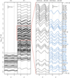 |
Fig. 12 Hertzsprung progression illustrated by the model RV curves of 208 fitted Cepheids (11 low-amplitude stars were removed for clarity). Cepheids are offset in the vertical direction according to their log Ppuls. Errorbars near the top show the constant velocity scale. Vertical dotted lines indicate ϕ = 0, the phase of minimum radius. Left panel, left column: Cepheids classified as first overtone pulsators in Gaia DR3. Left panel, right column: Cepheids classified as fundamental mode pulsators in Gaia DR3. Outliers with particularly small amplitudes are not shown for clarity (cf. Sect. 4.4). The shortest-period FU Cepheids is BP Cir. Right panels: close up view in the period range 9–18 days. Stars with double-peaked bump features are shown in blue on the right, stars with single-peaked bumps on the left in black. Names are color coded accordingly. Outliers Z Lac, CH Cas, and Y Oph are not shown for clarity. The double-peaked bump appears in 31/61 ≈ 50% of VELOCE Cepheids and may be a ubiquitous feature of Cepheid RV curves that requires very high precision and extremely dense phase sampling for detection. |
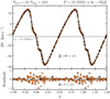 |
Fig. 13 VELOCE data and fit to XX Car, which exhibits a double-bumped descending RV branch. Only Coralie14 observations were used in this Fourier series fit employing 13 harmonics. The two peaks are clearly sampled. The data quality is sufficient to show the shortcoming of the Fourier series fit in reproducing the two bumps whose slopes are slightly less steep than implied by the fit to the overall RV curve. |
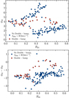 |
Fig. 14 Cepheids exhibiting double bumps on the declining RV curve part stand out in the ϕ41 vs. R21 diagram as a “connecting band” between two otherwise parallel sequences. In ϕ41 − ϕ31 vs. R21, double bump Cepheids also follow a significantly different trend. Plotting these parameters could serve to identify double bumps Cepheids in a quantitative manner rather than by visual inspection of the fits. |
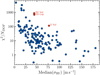 |
Fig. 15 Normalized χ2/NDOF of VELOCE Fourier series fits vs. the median uncertainty of the RV measurements for 151 non-SB1 Cepheids. The rapid increase of χ2/NDOF for precise measurements with typical uncertainties better than 20–40 m s−1 shows the existence of additional signals that are not reproduced by Fourier series models with constant Ppuls. The three longest-period Cepheids in the sample, GS Lup, SV Vul, and S Vul are labeled and highlighted. |
Cepheids exhibiting modulated variability.
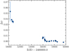 |
Fig. 16 Phase shifts vs. observation date for R Cru determined by template fitting. The long-term change in Δϕ is the signature of secular period change (cf. Sect. 5.3), whereas an oscillatory pattern among the VELOCE data is also clearly apparent. R Cru is the Cepheid with the shortest known orbital period in the MW, Porb = 237.6 days (cf. Paper II). |
4.4 Linear radius variations
The linear radius variation, ΔR = p ∫ υrdϕ, is calculated by integration of the RV curve over the pulsational cycle and by deprojecting observed line-of-sight velocities to the speed of radial displacement as seen from the star’s center using the projection factor p. We specify ΔR in solar radii assuming R⊙ = 695 700.0km as used in astropy. constants (version 5.3.4). ΔR is crucial to BW-type methods of distance determination (henceforth: BW distances), since the ratio of radial to angular diameter variation is proportional to distance. As pointed out by Anderson (2014), RV curve modulation (cf. Sect. 4.3) complicates the calibration of the projection factor, p, and the use of BW distances for Leavitt law calibration. Additionally, p is a very complex quantity that serves as a placeholder for several effects, including geometry, limb darkening, and atmospheric velocity gradients (e.g., Nardetto et al. 2007, 2017). Nevertheless, there is a strong interest in calibrating p for the distance scale, notably using interferometry and Gaia parallaxes (Breitfelder et al. 2016; Trahin et al. 2021). However, for the time being, no clear picture has arisen as to whether p should be considered a constant, or, e.g., dependent on Ppuls.
Here, we address the issue of determining ΔR solely from the observed RV curve by computing ΔR/p = ∫ υrdϕ from the homogeneously measured VELOCE data. This allows us to test whether p should be constant or a function of Ppuls without considering angular diameter variations, purely based on the consistency of ΔR/p at different values of log P.
Figure 17 shows the RV curve integrals obtained from the Fourier series fits to VELOCE data, ∫ υrdϕ = ΔR/p, against log P, and Fig. 18 shows the same information with dual logarithmic axes. The most striking feature in Fig. 17 is the sharp change in slope that occurs near Ppuls~10days. Assuming a constant value for p, this would imply that long-period (Ppuls > 10 days) Cepheids vary their size much more significantly than short-period Cepheids, and that the transition between long and short-period Cepheids is abrupt. While a break in RV amplitudes at 10.47 d was previously identified by Klagyivik & Szabados (2009), no reference to its significance for BW distances and p-factor calibration was made8.
Figure 17 distinguishes five groups of Cepheids: high-(Ap2p > 20 km s−1) and low-amplitude Cepheids with Ppuls<10 days, as well as three sequences of long-period Cepheids selected in an ad hoc fashion for further investigation. Among the short-period Cepheids, the selection according to Ap2p distinguishes relatively well between stars pulsating in the fundamental mode and the first overtone, despite some imperfections. As the right panel of Fig. 17 shows, there is a continuum of ΔR/p values between linear fits to the two groups of short-period Cepheids that grows increasingly wide with increasing log P. At Ppuls ≳ 10 days, Cepheids with low values of ΔR/p suddenly disappear.
We identified ad hoc three groups of long-period Cepheids using Fig. 17 and marked them via orange, green and yellow symbols. In the following, we refer to these three groups as the high- (yellow, largest ΔR/p), intermediate- (green, intermediate), and low-ΔR sequences (orange, smallest ΔR/p). The low-ΔR sequences sequence contains 11/82 = 13.4% of the Cepheids with P > 10 days, the intermediate sequence 15/82 = 18.3%, and the high-ΔR sequence the majority of Cepheids (56/82 = 68.3%). The names of the stars belonging to the low-ΔR sequence are annotated in Fig. 18. Curiously, we find Y Oph to lie on what appears to be the extension of FO Cepheids, together with ASAS J070747–2455.2, V0340 Nor, HW Car, and others. This is potentially noteworthy, as V0440 Per was previously identified as the longest-period overtone Cepheid in the MW (Baranowski et al. 2009).
To the best of our knowledge, the three ΔR/p sequences have not previously been investigated separately. While the assignment of a specific Cepheid to each sequence (in particular the intermediate one) may be questioned, the significant outlier nature of many long-Ppuls Cepheids from the (yellow) majority is obvious. Of course, the lower values of ΔR/p are a direct consequence of their lower peak-to-peak amplitudes, which are established here with high precision. In analogy to the amplitude cut applied to short-period Cepheids, we considered it useful to introduce the three sequences in order to investigate whether any differences would appear between stars on different ΔR/p sequences.
Interestingly, the slope of ΔR/p vs. log P steepens with increasing ΔR/p, resulting in a growing (absolute) difference in ΔR/p among the sequences towards the longest periods. However, the relative difference between the sequences decreases towards longer periods, from nearly 50% near 10 d to less than 25% near log P ~ 1.7. Assuming a strict dependence of the angular diameter variation on log P would therefore require very significant differences in p as a function of log P that may explain the difficulties encountered in the observational calibration of p, and these differences would become even more noticeable if a single relation is sought for p(log P). Interestingly, Fig. 8 in Trahin et al. (2021) exhibits such a trend, whereby the scatter in p grows towards lower log P and becomes particularly high around log P ~ 0.8.
In case these may be useful, the relations fitted to the five groups are listed in Table 4. Appendix A.1 contains figures that illustrate the Fourier parameters for all five groups, and Fig. 19 shows the ratio of the 4th to the 2nd harmonic amplitude (R41/R21) against ϕ41. An impressive discontinuity is seen among the yellow points around 3.5 ≲ ϕ41 ≲ 4.5, while the other long-period Cepheids shown in green and orange exhibit generally flat trends.
We considered several possible differences among the high-and low-ΔR sequences. The low-ΔR sequence contains both known (spectroscopic) binaries (YZ Car, RY Vel, RY Sco) and Cepheids with no known companions (e.g., ℓ Car, S Vul, Y Oph)9. Iron abundances compiled and homogenized by Groenewegen (2018) do not show a significant difference in the chemical composition of the three groups, cf. Fig. 20.
The color–magnitude diagram in Fig. 21 suggests that low-ΔR/p sequence stars may prefer a location slightly closer to the hot edge of the instability strip. However, we do not consider this preference significant at this time, and we do not find a similar preference for intermediate-ΔR sequence stars, nor a preference to avoid hotter temperatures among the high-ΔR sequence Cepheids. Nonetheless, we note that the hot instability strip boundaries of overtone Cepheids are located at slightly hotter temperatures than those of fundamental mode Cepheids (e.g., Anderson et al. 2016c). Distant outliers beyond the hot edge of the instability strip may have significant contamination by hot companion stars, although this remains unclear at the moment. Only one of the five most distant blue outliers is an SB1 Cepheids (in order of decreasing MV,0): T Ant, EZ Cyg, AS Vul, V0916 Aql (only SB1), and KX Cyg. The five outliers beyond the red instability strip boundaries (MV,0 < −4, in order of increasing MV,0) are VY Sgr (sole SB1 among red outliers), RS Nor, MQ Cam, V1019 Cas, and MN Cam. The reddest long-period Cepheid in the figure is XZ Car (an SB1).
Lastly, we considered the location of stars on the three ΔR sequences in the Leavitt law (LL). Figure 22 shows the reddening-free absolute Wesenheit magnitude (Madore 1982) in Gaia bands, WG = G − 1.911 • (GBp − GRp) computed using (inverted) Gaia DR3 Cepheid parallaxes corrected for parallax systematics quantified by (Lindegren et al. 2021) and the residual parallax offset of Gaia field Cepheids determined using cluster Cepheids10 (Cruz Reyes & Anderson 2023). Figure 22 shows that the low-ΔR sequence is not systematically populated by LL outliers. The notable exception is Y Oph, which is 7.1σ from the LL (Cruz Reyes & Anderson 2023, second row of their Table 11), has very small uncertainties, and appears to be consistent with the long-period extension of the first-overtone LL dominated by low-amplitude Cepheids. This is consistent with Y Oph following the trend of FO Cepheids in Fig. 18, despite its unusually long period. While none of the Gaia quality parameters indicate poor astrometry or photometry contaminated by a companion, we caution that its magnitude brighter than ⟨mG⟩ = 5.6 mag renders this star sensitive to saturation effects. Additionally, the Gaia parallax offsets at such bright magnitudes are not yet sufficiently characterized to ensure unbiased parallaxes for individual stars (Khan et al. 2023). Similarly, S Vul (⟨mG⟩ = 6.7 mag) is a ~3.9σ outlier from the MW LL. A few Cepheids consistent with the FO LL have Ap2p > 20 km s−1, whereas a few low-amplitude Cepheids also fall on the FU Cepheid LL. Hence, a simple distinction based on RV amplitude does not allow to conclusively assign pulsation modes.
In summary, the significant differences of ΔR/p between the three sequences are not due to companion stars, chemical composition, nor the incorrect assignment of the dominant pulsation modes, although some evidence points to the possibility that Y Oph may be pulsating in the first overtone. This leaves interactions between pulsation modes as well as atmospheric effects as possible origins of the reduced amplitudes and differences in ΔR/p. Further study is required to understand this issue, which significantly contributes to the complexity of p-factor calibration.
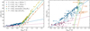 |
Fig. 17 RV curve integrals (=ΔR/p) vs. log P determined from the VELOCE best fit models. Short-period Cepheids (Ppuls < 10 days) are separated into low- and high-amplitude stars using a peak-to-peak RV threshold of 20 km s−1 and color coded in purple (≤ 20 km s−1) and blue (>20 km s−1). Long-period (P > 10d) FU Cepheids exhibit a strikingly (~5.6–6.6×) steeper trend than short-period Cepheids. We introduce an ad hoc distinction among three sequences for P > 10 d FU Cepheids into stars exhibiting large (yellow), intermediate (green), and small (orange) radius variations. The right panel shows a close-up view to more easily distinguish among short-period Cepheids, where a large number of Cepheids are found between the well-defined envelopes made up of FU and FO Cepheids, respectively. Stars near the edges are labeled to facilitate identification. |
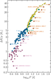 |
Fig. 18 Double-logarithmic plot of ΔR/p vs. Ppuls. All stars on the low-ΔR/p sequence are labeled. Color coding as in Fig. 17. |
Linear fits for the five subsets identified in the ΔR/p vs. log P relation.
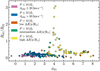 |
Fig. 19 Ratio of amplitudes between 4th and 2nd harmonic vs. ϕ41. Low ΔR/p stars have consistently low R42 more similar to short-period Cepheids, while high ΔR/p stars exhibit a very large range in R42 near 3.5 ≲ ϕ41 ≲ 4.5. |
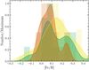 |
Fig. 20 Iron abundances compiled by Groenewegen (2018) for long-period Cepheids on the low- (orange), intermediate- (green), and high-ΔR/p (yellow) sequences introduced in Fig. 17. The binned histograms are superposed by KDE-smoothed distributions. No clear difference in metallicity is apparent between the three groups. |
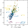 |
Fig. 21 Color magnitude diagram of VELOCE stars based on V- and K-band magnitudes and color excesses compiled by Groenewegen (2018), de-reddened using the Cardelli et al. (1989) reddening law. Color coding distinguishes between long-period Cepheids (Ppuls > 10 days) with low (orange), intermediate (green), and high (yellow) ΔR/p, as well as short-period (Ppuls < 10 days) high-RV amplitude (blue) and low-RV (purple). |
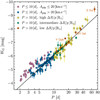 |
Fig. 22 Comparison of the stars belonging to the five subgroups in Fig. 17 shown in relation to the FU Cepheid MW Leavitt law calibrated using cluster Cepheids (Cruz Reyes & Anderson 2023, black solid line) and the reddening-free Wesenheit magnitude WG. Low-ΔR Cepheids are shown in orange and are not systematic outliers from the LL. The most significant outliers are Y Oph (7.1σ from the LL, ⟨mG⟩ = 5.5 mag) and S Vul (3.9σ, ⟨mG⟩ = 6.7 mag). The limitations of this comparison are described in the text. |
5 A legacy reference for Cepheid velocimetry
We determined systematic RV (zero-point) offsets of literature Cepheid RV datasets relative to VELOCE using a template fitting approach. The method is described in Sect. 5.1 and literature zero-point offsets are presented in Sect. 5.2. Cepheid RV templates based on principal component analysis are currently being prepared (Viviani et al., in prep.). Section 5.4 compares VELOCE data to Gaia DR3 time series RVs.
5.1 Template fitting of literature data
We employed a template fitting method previously developed in Anderson et al. (2016a); Anderson (2019) that fits our best-fit Fourier series models determined in Sect. 3.1 to literature time series of the same stars using two free parameters: the velocity offset relative to the VELOCE template and a phase shift. Figure 23 shows four examples of RV time series fitted using VELOCE templates of the same stars.
We split the available time series into time “clusters” according to data availability and quality using a nearly automated procedure based on kernel density estimates (KDE) as implemented in sklearn.neighbors (Pedregosa et al. 2011) in order to test time-variable offsets and to improve sensitivity to orbital motion. We typically used a bandwidth of at least 30 d, or 1 pulsation cycle, whichever is longer, unless either obvious rapid orbital motion made this impossible or the data were insufficient. In cases of very good data availability, we used bandwidths as short as one pulsation cycle, for example, when fitting VELOCE data. Figure 24 illustrates the procedure for four stars with different temporal sampling properties.
Each fitted data cluster contained at least three observations sufficiently spaced in pulsation phase in order to adequately constrain two fit parameters, Δυγ = υγ(t) − υγ,T and Δϕ = ϕ − ϕT, where subscript T refers to the values of the VELOCE template. Figure 16 shows the phase shifts determined for R Cru, the shortest-period SB1 Cepheid in the MW (cf. Paper II). Data clusters with insufficient number of observations were automatically discarded, and references with insufficient data for KDE clustering were considered as a single time series. We inspected all resulting template fits visually and modified starting conditions for Δϕ (very rarely Δυ) or the KDE bandwidth, if needed to obtain reasonable fits to the data.
For each clustered template fit, we recorded the reference, integer numbering of the data cluster, its mean date, its first and last observations, fit parameters Δυγ and Δϕ, as well as their uncertainties. We further recorded the time series of residuals of the data minus the template fit.
Template fitting results serve three main purposes: a) the estimation of zero-point offsets of literature data relative to VELOCE, b) the detection of temporal trends in υγ, and c) the determination of orbital solutions based on the longest available baselines. Here, we focus on element a) to facilitate the combination of VELOCE data with other datasets and to assess the quality of Gaia RVS time series of classical Cepheids published as part of DR3. Elements b) and c) are presented in Paper II. Additionally, the values of Δϕ allow for an estimation of the period changes, ![Mathematical equation: $\[\dot{P}\]$](/articles/aa/full_html/2024/06/aa48400-23/aa48400-23-eq9.png) , which we briefly discuss in Sect. 5.3.
, which we briefly discuss in Sect. 5.3.
5.2 Literature zero-point differences from template fitting
RV offsets between VELOCE and the literature are expected due to differences in wavelength calibration, wavelength ranges used to determine RV, and the growing accuracy of RV measurements over the many decades spanned by the literature data, among others.
We considered only well-observed and well-behaved11 non-SB1 Cepheids to determine zero-point differences. Using the clustered template fitting approach, we investigated possible temporal variations in the zero-points derived from multiple sources, cf. Fig. 25. Linear trends of Δυzp were investigated for all stars from the same reference. However, such trends were generally found to be negligible.
Since no significant evidence for temporal zero-point variations was found, we quantified the zero-point offset relative to VELOCE using the median Δυzp and the standard error on the median for each source. Table 5 lists the zero-point offsets relative to VELOCE derived for all references considered, and Fig. 26 shows the zero-point stability of Coralie07, Coralie14, and Hermes derived using the same approach. We stress that a large absolute value of Δυzp does not imply poor data quality.
Zero-points for Coralie and Hermes are reported in Sect. 2.5 alongside a discussion of zero-point changes due to instrument upgrades. This information will be used in the future to further improve the precision of VELOCE RV data and can serve to accurately tie our observations to other instruments and surveys. However, in this first data release, we considered a constant zero-point for Coralie and Hermes Cepheid RVs and worked under the hypothesis that both instruments had consistent zero-points. The fact that many Cepheids were observed with both instruments, and using each of the two instrument versions, allowed us to quantify the level of agreement of Coralie07, Coralie14, and Hermes with the overall VELOCE DR1 average. Using this approach, we recovered the correct sign and order of magnitude of the zero-point change (20 m s−1) between Coralie07 and Coralie14 (Sect. 2.5), albeit using high-amplitude variable stars instead of extremely stable RV standards. Conversely, we find Hermes to agree extremely closely with Coralie14. The Hermes zero-point change does not alter this picture significantly, since the majority of Hermes observations reported here were collected before the instrument upgrade.
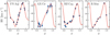 |
Fig. 23 Example template fits to literature data of stars with VELOCE RVs. Two parameters are fitted: the mean offset Δυγ and the phase offset Δϕ. The RV curve shapes and amplitudes are fixed by the VELOCE best fit models. From left to right: FN Aql observations by Barnes et al. (2005) closely fit to the VELOCE template; AX Cir observations by Lloyd Evans (1980) are sufficient to achieve a good template fit; BZ Cyg observations by Gorynya et al. (1992) show some scatter but the template fit is reliable thanks to dense phase sampling; even just seven VELOCE observations of R Mus allow for a precise template fit. |
 |
Fig. 24 Example of temporal data clustering based on KDE. The solid green lines indicate the kernel density estimate, and data are clustered temporally according to local KDE minima. From left to right: observations of S Cru by Gieren (1981) are insufficiently sampled for temporal clustering and used all together; observations of FF Aql by Gorynya et al. (1998) can and must be clustered during later epochs due to significant orbital motion; observations of KN Cen from VELOCE can be separated into several well-sampled data clusters; S Vul observations in VELOCE were separated into data clusters, although not all clusters could be used due to insufficient data points and rapid period fluctuations. |
Literature data discarded
Inspection of the template fits allowed us to identify individual unreliable RV observations reported in datasets from the literature. In particular, we identified two nights in the dataset by Borgniet et al. (2019) where the reported RV measurements differed by several km s−1 from expectations for 8 Cepheids. We therefore decided to remove all observations from the two nights of 24 and 25 June 2015 (reduced BJDs starting with 57198 and 57199) of that data set. We further discarded two observations for RU Sct reported by Bersier (2002, BJD around 57635.5) and one observation of BN Pup from the data reported by Storm et al. (2011) due to an offset of more than 20 km s−1 from the template fit.
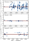 |
Fig. 25 Determination of RV zero-points as a function of time for different references. From top to bottom: Gorynya et al. (1998), the previously largest data set of classical Cepheid RV time series; Kienzle et al. (1999); Borgniet et al. (2019). Only stars with VELOCE observations are used to determine zero-points. Horizontal errorbars indicate the time span of the measurements. A solid red line shows an unweighted linear fit to investigate temporal trends; the dotted black line shows the median with its standard error as a grey shaded region. |
5.3 Period changes from RV template fitting
Cepheids exhibit a variety of period change phenomena, including linear period changes most likely due to secular evolution (e.g., Szabados 1989; Turner et al. 2006), oscillatory period changes (e.g., Kervella et al. 2017; Csörnyei et al. 2022), period “jitter” (e.g., Derekas et al. 2017), and possible sudden period changes (Turner et al. 2005). In particular the linear period changes are of interest for testing stellar evolutionary timescales (e.g., Turner et al. 2006; Fadeyev 2014; Anderson et al. 2016c; Miller et al. 2020) as they are expected to directly trace the monotonous (secular) evolution across the instability strip and allow for an identification of the instability strip crossing numbers according to the sign and magnitude of dP/dt = ![Mathematical equation: $\[\dot{P}\]$](/articles/aa/full_html/2024/06/aa48400-23/aa48400-23-eq10.png) (e.g., Anderson 2018a).
(e.g., Anderson 2018a).
The classical approach to measuring ![Mathematical equation: $\[\dot{P}\]$](/articles/aa/full_html/2024/06/aa48400-23/aa48400-23-eq11.png) performs O–C analysis (Sterken 2005) and compares the observed time of maximum light to the expected time of maximum light based on the known pulsation ephemerides. O–C is then usually plotted against Ncyc,E, the number of cycles12 elapsed since the reference epoch used to determine Ppuls, and fitted by a parabola13
performs O–C analysis (Sterken 2005) and compares the observed time of maximum light to the expected time of maximum light based on the known pulsation ephemerides. O–C is then usually plotted against Ncyc,E, the number of cycles12 elapsed since the reference epoch used to determine Ppuls, and fitted by a parabola13
![Mathematical equation: $\[\mathrm{O-C}=\frac{1}{2} \frac{\mathrm{d} P}{\mathrm{~d} t} \cdot P_{\text {puls }} \cdot N_{\mathrm{cyc}, \mathrm{E}}^2,\]$](/articles/aa/full_html/2024/06/aa48400-23/aa48400-23-eq12.png) (4)
(4)
where Ppuls denotes the period at the reference epoch, E. Using O–C = Δϕ • P and Ncyc,P = (BJD − E)/P, we determine ![Mathematical equation: $\[\dot{P}\]$](/articles/aa/full_html/2024/06/aa48400-23/aa48400-23-eq15.png) directly from this relation for 146 Cepheids with VELOCE and literature RV data using the measured values of Δϕ, P, and E. In almost all instances, the small baseline yielded |Δϕ| < 1. In a few cases, sudden steps in the Δϕ measurement sequence suggested that a full cycle had been skipped, and we added ±1 as needed to maintain a monotonous long-term period evolution.
directly from this relation for 146 Cepheids with VELOCE and literature RV data using the measured values of Δϕ, P, and E. In almost all instances, the small baseline yielded |Δϕ| < 1. In a few cases, sudden steps in the Δϕ measurement sequence suggested that a full cycle had been skipped, and we added ±1 as needed to maintain a monotonous long-term period evolution.
Table 6 lists the values of ![Mathematical equation: $\[\dot{P}\]$](/articles/aa/full_html/2024/06/aa48400-23/aa48400-23-eq16.png) thus determined and their formal uncertainties based on the covariance matrix of the weighted fit, as well as notes for individual stars to help the interpretation of our results. Among the available sample of 146,
thus determined and their formal uncertainties based on the covariance matrix of the weighted fit, as well as notes for individual stars to help the interpretation of our results. Among the available sample of 146, ![Mathematical equation: $\[\dot{P}\]$](/articles/aa/full_html/2024/06/aa48400-23/aa48400-23-eq17.png) is detected at 3σ significance or better for 80 stars, 39 (49%) of which have negative
is detected at 3σ significance or better for 80 stars, 39 (49%) of which have negative ![Mathematical equation: $\[\dot{P}\]$](/articles/aa/full_html/2024/06/aa48400-23/aa48400-23-eq18.png) . Counting all stars does not significantly change these statistics (53% negative
. Counting all stars does not significantly change these statistics (53% negative ![Mathematical equation: $\[\dot{P}\]$](/articles/aa/full_html/2024/06/aa48400-23/aa48400-23-eq19.png) ). This is rather different from large samples of photometrically measured
). This is rather different from large samples of photometrically measured ![Mathematical equation: $\[\dot{P}\]$](/articles/aa/full_html/2024/06/aa48400-23/aa48400-23-eq20.png) , such as the compilation of 196 Cepheids by Turner et al. (2006) that lists 33% negative and 67% positive
, such as the compilation of 196 Cepheids by Turner et al. (2006) that lists 33% negative and 67% positive ![Mathematical equation: $\[\dot{P}\]$](/articles/aa/full_html/2024/06/aa48400-23/aa48400-23-eq21.png) values and the recent study by Csörnyei et al. (2022), which reports 44/141 (31%) negative and 69% (97/141) positive
values and the recent study by Csörnyei et al. (2022), which reports 44/141 (31%) negative and 69% (97/141) positive ![Mathematical equation: $\[\dot{P}\]$](/articles/aa/full_html/2024/06/aa48400-23/aa48400-23-eq22.png) values.
values.
Figure 27 illustrates the values of ![Mathematical equation: $\[\dot{P}\]$](/articles/aa/full_html/2024/06/aa48400-23/aa48400-23-eq23.png) thus determined, separated into negative and positive
thus determined, separated into negative and positive ![Mathematical equation: $\[\dot{P}\]$](/articles/aa/full_html/2024/06/aa48400-23/aa48400-23-eq24.png) for stars for which
for stars for which ![Mathematical equation: $\[|\dot{P}|>3 \sigma_{\dot{P}}\]$](/articles/aa/full_html/2024/06/aa48400-23/aa48400-23-eq25.png) . Theoretical predictions from Fadeyev (2014) and Anderson et al. (2016c), as well as
. Theoretical predictions from Fadeyev (2014) and Anderson et al. (2016c), as well as ![Mathematical equation: $\[\dot{P}\]$](/articles/aa/full_html/2024/06/aa48400-23/aa48400-23-eq26.png) values determined by Csörnyei et al. (2022) using very long photometric time series are shown for comparison. Overall, we find very good agreement with both the models and the literature
values determined by Csörnyei et al. (2022) using very long photometric time series are shown for comparison. Overall, we find very good agreement with both the models and the literature ![Mathematical equation: $\[\dot{P}\]$](/articles/aa/full_html/2024/06/aa48400-23/aa48400-23-eq27.png) values. Given that much fewer RV observations than photometric observations are available in the literature, this can be considered a success. A more detailed study of period changes is, however, outside the scope of this work.
values. Given that much fewer RV observations than photometric observations are available in the literature, this can be considered a success. A more detailed study of period changes is, however, outside the scope of this work.
Despite this promising result, we caution that the values of ![Mathematical equation: $\[\dot{P}\]$](/articles/aa/full_html/2024/06/aa48400-23/aa48400-23-eq33.png) are subject to a few important caveats and complicating factors. Figure 16 illustrates this for R Cru, which exhibits both short-timescale non-linear period changes and a long-term linear trend in period. The non-linear period changes dominate over the baseline of VELOCE data, and the older data are required to improve sensitivity to the secular (linear) period change. Unfortunately, there are often long gaps between the sampled epochs and the older epochs are often few and not sufficient to resolve short-timescale variations at previous epochs. Fitting the long-term trend using the above parabolic model can thus occasionally produce a biased result, since a) the VELOCE epochs will dominate the fit due to higher number of epochs and high precision and b) the effect of non-linear period changes on the older epochs cannot be assessed. Issues related to non-linear period changes can be expected to occur more frequently and severely in long-period fundamental-mode and short-period first-overtone Cepheids, whose Ppuls are known to be less stable than those of short-period fundamental mode Cepheids (e.g., Anderson 2014; Süveges & Anderson 2018b; Csörnyei et al. 2022). The last column of Table 6 provides further guidance for our results.
are subject to a few important caveats and complicating factors. Figure 16 illustrates this for R Cru, which exhibits both short-timescale non-linear period changes and a long-term linear trend in period. The non-linear period changes dominate over the baseline of VELOCE data, and the older data are required to improve sensitivity to the secular (linear) period change. Unfortunately, there are often long gaps between the sampled epochs and the older epochs are often few and not sufficient to resolve short-timescale variations at previous epochs. Fitting the long-term trend using the above parabolic model can thus occasionally produce a biased result, since a) the VELOCE epochs will dominate the fit due to higher number of epochs and high precision and b) the effect of non-linear period changes on the older epochs cannot be assessed. Issues related to non-linear period changes can be expected to occur more frequently and severely in long-period fundamental-mode and short-period first-overtone Cepheids, whose Ppuls are known to be less stable than those of short-period fundamental mode Cepheids (e.g., Anderson 2014; Süveges & Anderson 2018b; Csörnyei et al. 2022). The last column of Table 6 provides further guidance for our results.
Literature zero-point offsets relative to VELOCE.
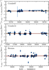 |
Fig. 26 RV zero-point stability for the three instruments distinguished here, Coralie07, Coralie14, and Hermes relative to the overall VELOCE zero-point set by the combined dataset of all Cepheids, which includes stars observed with both Coralie versions, as well as with Hermes and Coralie. The vertical scale and color scheme is identical to Fig. 25. Horizontal errorbars indicate the time span of the measurements. Outliers from the median are mostly due to imperfect template fits or low-amplitude signals mimicking temporal variations in υγ. The Hermes zero-point change due to the intervention in 2018 is visible near BJD 58300, cf. Table 1. |
Linear rates of period change, ![Mathematical equation: $\[\dot{P}\]$](/articles/aa/full_html/2024/06/aa48400-23/aa48400-23-eq28.png) measured by RV template fitting (extract).
measured by RV template fitting (extract).
5.4 Gaia DR3 RV measurements from the RVS instrument
On 13 June 2022, 43 298 time series radial velocity measurements obtained with the Gaia Radial Velocity Spectrometer (henceforth: Gaia RVs) became available as part of the third Gaia data release (Katz et al. 2023). Among these are 15 171 time series observations of 731 classical Cepheids (stars labeled ‘DCEP’ in column type_best_classification of Gaia DR3 table gaiadr3.vari_cepheid). Gaia RVs are of particular interest given their great number, the large sample of stars (Ripepi et al. 2023), and the growing number of epochs being collected as the mission progresses. For Cepheids, the mean per-epoch Gaia RVs uncertainty is 2.0 km s−1 (median 1.4 km s−1, standard deviation 2.1 km s−1). The most precise Gaia RV observation has an uncertainty of 0.135 km s−1, and the least precise 46.8 km s−1. The mean number of observations per star is 21 (gaiadr3.vari_cepheid table num_clean_epochs_rv), with a full range of 4–74. The mean reported uncertainties for pulsation averaged velocities, υγ, according to table gaiadr3.vari_cepheid is 1.9 km s−1 (median 1.5 km s−1, standard deviation 2.3 km s−1, full range 0.03–25 km s−1), somewhat larger than the typical uncertainties reported by Ripepi et al. (2023, 1–1.5 km s−1). Thus, Gaia RVs are available for a 2.8× larger sample than VELOCE, albeit with typically fewer (~half) observations per target, shorter baselines, and significantly (~30×) lower precision. Importantly, Gaia RVs are fully contemporaneous with VELOCE, offering a unique opportunity for direct comparisons with minimal complications due to orbital motion or variable ephemerides.
The number of Gaia observations are set to grow substantially as Gaia completes its unprecedented survey, and the final Gaia data release will feature similar temporal baselines as VELOCE. However, there are several important systematic differences in the way that RVs are measured here and using Gaia. The following investigates these differences, first using the RV time series (Sect. 5.4.1), followed by a comparison of the values of υγ and peak-to-peak amplitude derived by Ripepi et al. (2023) using Fourier series models (Sect. 5.4.2).
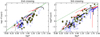 |
Fig. 27 Double-logarithmic plot of linear period changes, |
![Mathematical equation: $\[\dot{P}\]$](/articles/aa/full_html/2024/06/aa48400-23/aa48400-23-eq34.png)
![Mathematical equation: $\[|\dot{P}| / \sigma_\dot{p} \geq 3\]$](/articles/aa/full_html/2024/06/aa48400-23/aa48400-23-eq35.png)
![Mathematical equation: $\[\dot{P}\]$](/articles/aa/full_html/2024/06/aa48400-23/aa48400-23-eq36.png)
![Mathematical equation: $\[\dot{P}\]$](/articles/aa/full_html/2024/06/aa48400-23/aa48400-23-eq37.png)
![Mathematical equation: $\[\dot{P}\]$](/articles/aa/full_html/2024/06/aa48400-23/aa48400-23-eq38.png)
5.4.1 Template fitting of Gaia RVS time series observations
We investigated the overall zero-point offset of Gaia RVs relative to VELOCE by fitting the Gaia RV time series observations using VELOCE templates, analogous to Sect. 5.1. Figure 28 illustrates the examples of four stars. The top row illustrates template fits to the full Gaia RVs time series for SS CMa (left), as well as template fits to two time clusters made up of the same data set (center and right). The bottom row illustrates three additional stars with different RV curve shapes and amplitudes. The largest differences are seen near the extremes of the RV curve and near bump features, which appear visibly different from the VELOCE templates of RV curves measured using optical lines. We surmise that this effect arises primarily due to the different behavior of the lines near the Ca II triplet compared to the metallic line RVs reported in the Cepheid literature and in VELOCE (e.g., Wallerstein et al. 2019; Hocdé et al. 2020).
Figure 29 compares the values of ![Mathematical equation: $\[v_{\gamma, \mathrm{GDR} 3}^{\star}\]$](/articles/aa/full_html/2024/06/aa48400-23/aa48400-23-eq39.png) , determined here by template fitting to the Gaia RV time series measurements, to υγ,GDR3, the constant term of the Fourier series fitted to Gaia RVs data as part of the SOS processing (Clementini et al. 2023; Ripepi et al. 2023, parameter average_rv in table gaiadr3.vari_cepheids). Overall, we found good agreement between the two υγ values over the full range from −80 km s−1 to + 100 km s−1, with an rms of 1.9 km s−1.
, determined here by template fitting to the Gaia RV time series measurements, to υγ,GDR3, the constant term of the Fourier series fitted to Gaia RVs data as part of the SOS processing (Clementini et al. 2023; Ripepi et al. 2023, parameter average_rv in table gaiadr3.vari_cepheids). Overall, we found good agreement between the two υγ values over the full range from −80 km s−1 to + 100 km s−1, with an rms of 1.9 km s−1.
To quantify the offset of Gaia RVs relative to VELOCE, we measured the differences in υγ resulting from the template fit minus the VELOCE pulsation-averaged velocity, ![Mathematical equation: $\[\Delta v_{\gamma, \mathrm{GDR} 3}^{\star}=v_{\gamma, \mathrm{GDR} 3}^{\star}-v_{\gamma, \mathrm{VELOCE}}\]$](/articles/aa/full_html/2024/06/aa48400-23/aa48400-23-eq40.png) . We first used the full Gaia RVs time series at once and then repeated the procedure using KDE clustering to investigate temporal trends. The clustered approach using 121 estimates of 62 Cepheids with precise template fits
. We first used the full Gaia RVs time series at once and then repeated the procedure using KDE clustering to investigate temporal trends. The clustered approach using 121 estimates of 62 Cepheids with precise template fits ![Mathematical equation: $\[\left(\sigma_{\Delta v_\gamma} \leq\right.\left.~0.5 \mathrm{~km} \mathrm{~s}^{-1}\right)\]$](/articles/aa/full_html/2024/06/aa48400-23/aa48400-23-eq41.png) yielded a median offset of Δυγ = 0.65 ± 0.11 km s−1 (dispersion 0.92 km s−1) and is reported in Table 5. Relaxing the constraint on precision to
yielded a median offset of Δυγ = 0.65 ± 0.11 km s−1 (dispersion 0.92 km s−1) and is reported in Table 5. Relaxing the constraint on precision to ![Mathematical equation: $\[\sigma_{\Delta v_\gamma} \leq 1.0 \mathrm{~km} \mathrm{~s}^{-1}\]$](/articles/aa/full_html/2024/06/aa48400-23/aa48400-23-eq42.png) yielded 151 estimates of 74 Cepheids and a similar offset of 0.67 ± 0.12 (dispersion 1.15 km s−1). Considering the entire time series for all 66 Cepheids with
yielded 151 estimates of 74 Cepheids and a similar offset of 0.67 ± 0.12 (dispersion 1.15 km s−1). Considering the entire time series for all 66 Cepheids with ![Mathematical equation: $\[\sigma_{\Delta v_\gamma} \leq 0.5 \mathrm{~km} \mathrm{~s}^{-1}\]$](/articles/aa/full_html/2024/06/aa48400-23/aa48400-23-eq43.png) at once yielded the consistent, albeit slightly less precise, result of 0.70 ± 0.15 km s−1 (σ = 1.00 km s−1). Including less precise template fits
at once yielded the consistent, albeit slightly less precise, result of 0.70 ± 0.15 km s−1 (σ = 1.00 km s−1). Including less precise template fits ![Mathematical equation: $\[\left(\sigma_{\Delta v_\gamma} \leq 1.0 \mathrm{~km} \mathrm{~s}^{-1}\right)\]$](/articles/aa/full_html/2024/06/aa48400-23/aa48400-23-eq44.png) changes this to 76 Cepheids and a median offset of 0.77 ± 0.17 km s−1.
changes this to 76 Cepheids and a median offset of 0.77 ± 0.17 km s−1.
Figure 30 illustrates the clustered results and exhibits an initially surprising degree of scatter ranging from ![Mathematical equation: $\[-1 \lesssim \Delta v_{\gamma, \mathrm{GDR} 3}^{\star} \lesssim3 \mathrm{~km} \mathrm{~s}^{-1}\]$](/articles/aa/full_html/2024/06/aa48400-23/aa48400-23-eq48.png) . This range is larger when including less precise template fits. The large scatter partially arises due to the use of different synthetic spectra for every star in the Gaia RVS cross-correlation pipeline (Katz et al. 2023). For stars brighter than gRVS ≤ 12 mag (Sartoretti et al. 2023), the choice of template is decided automatically in favor of the spectral template that consistently yields the highest correlation peaks. This approach is well adapted for dealing with the enormous number and diversity of objects observed by Gaia. However, when comparing RVs of a group of similar objects, such as Cepheids, it is advantageous to adopt the same correlation mask for all stars in the group and their spectra in order to ensure consistent RV zero-points. Choosing different templates either from Cepheid to Cepheid, or as a function of phase for the same Cepheid, may complicate the interpretation of the results because different correlation templates assign different weights to the same spectral lines.
. This range is larger when including less precise template fits. The large scatter partially arises due to the use of different synthetic spectra for every star in the Gaia RVS cross-correlation pipeline (Katz et al. 2023). For stars brighter than gRVS ≤ 12 mag (Sartoretti et al. 2023), the choice of template is decided automatically in favor of the spectral template that consistently yields the highest correlation peaks. This approach is well adapted for dealing with the enormous number and diversity of objects observed by Gaia. However, when comparing RVs of a group of similar objects, such as Cepheids, it is advantageous to adopt the same correlation mask for all stars in the group and their spectra in order to ensure consistent RV zero-points. Choosing different templates either from Cepheid to Cepheid, or as a function of phase for the same Cepheid, may complicate the interpretation of the results because different correlation templates assign different weights to the same spectral lines.
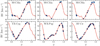 |
Fig. 28 Example VELOCE model template fits to Gaia RVs. Top row: the full set of Gaia RVs for SS CMa is fitted at once (left) or split into two epoch (center and right). gaiadr3.gaia_source does not provide the template parameters for SS CMa despite Gaia RVs being available in gaiadr3.vari_epoch_rv. Bottom row: stars whose Gaia RVs were determined using different temperatures (from left to right: TX Cyg (4250K), WX Pup (5250K), AV Cir (6250K)). VELOCE uses a correlation mask created to match spectral type G2. |
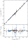 |
Fig. 29 Comparison of Gaia DR3 parameter average_rv from table gaiadr3.vari_Cepheid, υγ,GDR3, to the pulsation-averaged velocity derived by template fitting of the Gaia DR3 RV time series, |
![Mathematical equation: $\[v_{\gamma, \mathrm{GDR} 3}^{\star}\]$](/articles/aa/full_html/2024/06/aa48400-23/aa48400-23-eq45.png)
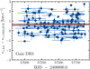 |
Fig. 30 Differences between |
![Mathematical equation: $\[v_{\gamma, \mathrm{GDR} 3}^{\star}\]$](/articles/aa/full_html/2024/06/aa48400-23/aa48400-23-eq46.png)
![Mathematical equation: $\[\left|\sigma_{\Delta v_\gamma}\right| \leq0.5 \mathrm{~km} \mathrm{~s}^{-1}\]$](/articles/aa/full_html/2024/06/aa48400-23/aa48400-23-eq47.png)
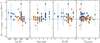 |
Fig. 31 Difference Δυγ = υγ,GDR3−υγVELOCE between parameter average_rv from gaiadr3.vari_cepheid and υγ from VELOCE for 71 well-behaved non-SB1 Cepheids as a function of the Gaia correlation template parameters and the number of Gaia time series observations, num_clean_epochs_rv. Orange points highlight the 33 Cepheids whose Gaia RVs were measured using the most suitable template parameter range 5000 ≤Teff ≤ 6500, log g ≤ 2, and −0.75 ≤ [Fe/H] ≤ 0.75. The green point in the right-most panel is RW Cas, for which the template parameters are not known. Trends appear among all template parameters, with cooler templates or higher-log g templates yielding larger positive offset. RVs measured using adequate template parameters show significantly improved scatter. |
5.4.2 Comparison of Gaia RVS Fourier fit results to VELOCE
We considered the parameters average_rv and peak_to_peak_rv from table gaiadr3.vari_cepheid to investigate the impact of template parameters on the offset between Gaia and VELOCE. The spectral template parameters rv_template_teff, rv_template_logg, and rv_template_fe_h were taken from table gaiadr3.source_id, and are available for the majority of stars with Gaia RV time series measurements or average_rv values, but not all (exceptions include RW Cas, SS CMa, and BM Per). We considered the range 5000 < Teff [K] < 6500, log g ≤ 2.0, and −0.75 ≤ [Fe/H] ≤ 0.75 to be particularly adequate for Cepheids and distinguish Gaia results based on this range in the following as orange points.
Figure 31 shows Δυγ,GDR3 = υγ,GDR3−υγVELOCE against the correlation template parameters for 71 stars, 33 of which were processed using the most adequate range of template parameters. Trends can be seen among all three template parameters, although their relative contributions are not immediately distinguished. The most obvious trend in Fig. 31 is that υγGDR3 is much more consistent with VELOCE when the adequate template parameter range is considered. In this case, just over ≳10 measurements suffice to find a similar result (±2 km s−1). When the full parameter range is considered, a larger number of observations is required. Figure 31 also suggests that the automated identification of the appropriate parameter range works best when a larger number of observations are available (≳25).
Figure 32 shows the ratio between the peak-to-peak RV amplitudes from Gaia and VELOCE as a function of the Gaia correlation template parameters and Nobs,GDR3. Interestingly, neither the number of observations, nor the choice of template parameters appears to significantly affect this comparison. We did not find significant evidence of biased amplitudes, although there is a noticeable dispersion of ~16% between the amplitudes. For the time being, it remained unclear whether this is a physical effect related to the amplitudes of near-IR lines, or the precision of Gaia peak-to-peak amplitudes, since the number of harmonics used to fit Gaia RV curves was likely low (2–3; G. Clementini, priv. comm.) and is not reported in the vari_cepheids table. Larger number of observations in the next Gaia DR4 will allow for a more detailed comparison of amplitudes. In the meantime, we caution that inferences sensitive to RV amplitudes, such as BW-type distances or p-factor calibrations, will be limited by the dispersion seen in Fig. 32.
Figure 33 illustrates the differences shown in Figs. 31 and 32 as a function of log P. At a pivot period of Ppuls = 10 days (log P = 1), the median offset if 0.51 ± 0.13 km s−1, consistent with the offset determined using template fitting. Additionally, a trend of 1.03 ± 0.29 km s−1/log P (3.5σ) trend is found. A larger offset of 1.6 ± 0.2 km s−1 and steeper trend of 1.69 ± 0.44 km s−1/log P (3.8σ) is found among the stars whose template parameters were outside the most adequate range (blue points). As seen in Fig. 32, the amplitude ratio appears very stable across the full range of periods. We tentatively note better agreement for short-period Cepheids processed with the adequate template parameters (log P ≲ 0.7), although a cleaner comparison would required a larger number of stars.
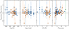 |
Fig. 32 Ratio of the peak-to-peak RV amplitudes from Gaia DR3 (peak_to_peak_rv from table gaiadr3.vari_cepheid) to the VELOCE peak-to-peak RV amplitudes as a function of the template parameters, analogous to Fig. 31. The amplitude ratios exhibit large scatter. However, no clear trends emerge. |
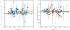 |
Fig. 33 υγ (left) and peak-to-peak RV amplitude (right) determined by Gaia SOS compared to VELOCE as a function of logarithmic pulsation period. υγ,GDR3 and Ap2p,GDR3 are the values published in table gaiadr3.vari_cepheid as parameters average_rv and peak_to_peak_rv, respectively. Orange points highlight Cepheids for which Gaia used the most adequate template parameters. Blue points show measurements processed using template parameters outside this range. Blue and orange solid lines show linear fits to the respective points; green solid lines show linear fits to the combined data sets. At log P = 1, we find Δυγ = 0.51 ± 0.13 km s−1, and a slight trend of 1.03 ± 0.29 km s−1/log P for the orange points. The blue points exhibit a much more significant offset of 1.6 ± 0.2 km s−1 and trend 1.69 ± 0.44 km s−1 / log P. Peak-to-peak amplitudes are generally consistent with a dispersion of approximately 16% and do not exhibit a trend with log P. |
6 Summary and conclusions
We present the first data release (DR1) of the VELOCE project, which comprises more than 18 225 high-precision radial velocity measurements of 253 classical Cepheids located on both hemispheres, as well as 1161 observations of 164 stars that are not classical Cepheids. This data set provides an unprecedented combination of RV precision (median uncertainty of 0.037 m s−1), sample size, and temporal baselines of up to 11 yr featuring well-characterized RV zero-points based on RV standard stars. VELOCE extends the number of Cepheid RV time series at magnitudes fainter than G ≳ 10 mag, where previous catalogs contained relatively few observations. Systematic zero-point changes following instrumental upgrades (~26 m s−1 on Coralie, <75 m s−1 on Hermes) have been characterized.
We performed Fourier decomposition of RV curves with an emphasis on model selection and to determine ephemerides from the RV data directly. Contrary to common practice, we define ϕ = 0 at minimum radius, since this phase is most precisely measurable. The fitted Fourier series models provide the most detailed view of the Hertzsprung (1926) progression of MW Cepheids to date and revealed a second bump feature on the descending RV branch of approximately half of the observed Cepheids with periods between 9–18 days. These double bumps are likely to further inform mode resonances (Simon & Lee 1981; Buchler et al. 1990; Antonello & Morelli 1996), and further investigation of this feature is required to understand their potential for informing the evolution and pulsation physics of Cepheids.
Approximately 30% of the Cepheids studied here exhibit changes in the pulsation-averaged velocity, υγ, due to orbital motion. A systematic study of spectroscopic binaries is presented in Paper II of this series (Shetye et al., in prep.).
Thirty-six Cepheids were found to exhibit various forms of modulated variability, that is, variability signals beyond the dominant pulsation mode or orbital motion (not counting doublemode Cepheids). The dichotomy of long-timescale modulations among overtone Cepheids and cycle-to-cycle variations for long-period Cepheids reported by Anderson (2014) is confirmed. Modulated variability becomes ubiquitous for given sufficient RV precision (20–40 m s−1 per epoch), and the diversity of phenomena suggests that multiple astrophysical mechanisms are at play. High-precision RV observations of Cepheids thus hold great promise to cast open an asteroseismic window for studying this advanced evolutionary stage of intermediate-mass stars in unprecedented detail. Future work will systematically study this “modulation zoo,” starting with the discovery of non-radial pulsation in Cepheid time series spectra (Netzel et al. 2024).
We investigated the linear radius variations and found striking differences in the RV curve integrals (ΔR/p) between Cepheids with Ppuls above and below 10 days. We noted at least two, possibly three, distinct sequences of long-period Cepheids (P > 10 days) in the ΔR/p vs. log P diagram, which we conjecture are at the origin of the difficulties encountered when calibrating BW-type projection factors. Although no obvious physical explanation for these sequences was identified, we noticed mild preference for the sample of 11 Cepheids exhibiting the smallest linear radius variations (the low-ΔR/p sequence) to reside not far from the blue edge of the instability strip (Fig. 21).
The VELOCE project provides a legacy dataset of high-quality Cepheid RVs that will enable further study and allow for future datasets to be combined with existing ones from the literature. All RV time series measurements and the results from Fourier series modeling of single-mode bona fide Cepheids are made publicly available in this data release (DR1). To facilitate accurate comparisons with the literature, we have determined RV zero-point offsets relative to the VELOCE zero-point for 31 literature sources using a template fitting approach. This also allowed us to measure secular (linear) period changes of 80 Cepheids based on RV measurements alone. We found good agreement with photometrically measured linear period changes from the literature as well as stellar model predictions.
Comparing our template fitting results to recently published Gaia DR3 time series measurements, we find an average offset from VELOCE of 0.65 ± 0.12 km s−1. Systematic offsets of a few to several km s−1 were found for stars whose RVs were measured using inadequate template parameters. The published RV amplitudes of Cepheids in Gaia DR3 exhibit significant (16%) scatter around the closely mapped VELOCE amplitudes. As Gaia continues its unprecedented survey of the MW, the number of published RV time series measurements are set to skyrocket. To ensure consistency among the measurements for specific variable star classes, we recommend using predefined sets of correlation template parameters for classes of large-amplitude variables, such as Cepheids. The accuracy of RV peak-to-peak amplitudes is likely to improve as more epochs are being collected. Ensuring the consistency of RV amplitudes measured by Gaia’s RVS instrument with angular diameter variations will be paramount to achieving accurate BW projection factor calibrations based on hundreds, if not thousands, of Cepheids.
Acknowledgements
This work would not have been possible without a great deal of help from a large number of people. Useful with discussions with the following people are acknowledged (in alphabetical order): Gisella Clementini, Xavier Dumusque, Nancy R. Evans, Michel Grenon, Martin Groenewegen, Pierre Kervella, Christophe Lovis, Antoine Mérand, Francesco Pepe, Vincenzo Ripepi, Damien Ségransan, Jesper Storm, Laszlo Szabados, Stéphane Udry. We especially thank the support staff at Euler, Mercator, La Silla Observatory, the Observatorio del Roque de los Muchachos, at the University of Geneva, KU Leuven, and ESO for their excellence and dedication to operating and maintaining these facilities. This notably includes Luc J. M. Weber, René Debusson, Michel Fleury, Michel Crausaz, Gregory Lambert, Vincent and Denis Mégevand, Gaspare Lo Curto, Emmanuela Pompei, Jesus Dalgado, Florian Merges, among others. We also warmly thank the following people for contributing observations on Euler and/or Mercator: Maxime Spano, Pierre Dubath, Thierry Semaan, Maria Süveges, Mihaly Varadi, Janis Hagelberg, Nicolas Cantale, Sarah Gebruers, Maddalena Bugatti, Amaury M. J. Triaud, Abigail Frost, Marion Cointepas, Monika Lendl, Dominique Naef, Matthias Fabry, Sébastien Peretti, Uriel Conod, Julia Seidel, Siemen Burssens, Raine Karjalainen, Azzurra Bigioli, Federica Cersullo, Ga el Ottoni, Thibault Merle, Olivier Verhamme, Akke Corporaal, Bruno Chazelas, Fatemeh Motalebi, Javiera Rey Cerda, Rosemary Mardling, Nicolas Lodieu, Tinne Pauwels, Lea Planquart, Steven Bloemen, Beatriz Gonzalez Merino, Oliver Turner, and Sara Mancino, among others. While we sought to include everyone who contributed, we are likely to have forgotten some, and we apologize to those we failed to mention. Your contributions were nonetheless valuable! We thank the anonymous referee for a constructive report that helped to improve the manuscript. This research has received support from the European Research Council (ERC) under the European Union’s Horizon 2020 research and innovation programme (Grant Agreement No. 947660). RIA and SK are funded by the SNSF Swiss National Science Foundation Eccellenza Professorial Fellowship (award PCEFP2_194638). RIA acknowledges funding and support from several sources over the 11 yr duration of the project, including the Swiss National Science Foundation early Postdoc. Mobility fellowship (grant No. 155687) and the ESO fellowship program in Garching. AT is a Research Associate at the Belgian Scientific Research Fund (F.R.S.-F.N.R.S.). MP is supported by BEKKER fellowship BPN/BEK/2022/1/00106 from the Polish National Agency for Academic Exchange. The Euler telescope is funded by the Swiss National Science Foundation (SNSF). Early VELOCE observations (2010–2016) were enabled by SNSF project funding from grant Nos. 119778, 130295, and 140893. MM acknowledges the support of the Swiss National Science Foundation (SNSF) under grant P500PT_203114. This research is based on observations made with the Mercator Telescope, operated on the island of La Palma by the Flemish Community, at the Spanish Observatorio del Roque de los Muchachos of the Instituto de Astrofísica de Canarias. Hermes is supported by the Fund for Scientific Research of Flanders (FWO), Belgium, the Research Council of K.U. Leuven, Belgium, the Fonds National de la Recherche Scientifique (F.R.S.-FNRS), Belgium, the Royal Observatory of Belgium, the Observatoire de Geneève, Switzerland, and the Thüringer Landessternwarte, Tautenburg, Germany. This research was supported by the International Space Science Institute (ISSI) in Bern, through ISSI International Team project #490, SHoT: The Stellar Path to the Ho Tension in the Gaia, TESS, LSST and JWST Era. This research has made use of NASA’s Astrophysics Data System; the SIMBAD database and the VizieR catalog access tool provided by CDS, Strasbourg; Astropy, a community-developed core Python package for Astronomy (Astropy Collaboration 2013, 2018).
Appendix A Classical Cepheids in VELOCE
Here, we report the list of classical Cepheids in this first VELOCE data release. Table A.1 lists identifiers, coordinates, Gaia DR3 information (source ids, mean G-band magnitudes, mean ![Mathematical equation: $\[G_{B p}-G_{R p}\]$](/articles/aa/full_html/2024/06/aa48400-23/aa48400-23-eq49.png) color, and pulsation modes), whether the star exhibits orbital motion based on VELOCE data alone (not considering literature information, which is included in Paper II), the number of VELOCE observations, the number of Fourier harmonics used in the modeling, NFS, the pulsation period Ppuls, its uncertainty (squared sum of statistical and systematic error), and the epoch of minimum radius E with its uncertainty (squared sum of statistical and systematic error). All information presented in Tab. A.1 is contained within the data files provided via Zenodo14 in FITS format, cf. App. C.
color, and pulsation modes), whether the star exhibits orbital motion based on VELOCE data alone (not considering literature information, which is included in Paper II), the number of VELOCE observations, the number of Fourier harmonics used in the modeling, NFS, the pulsation period Ppuls, its uncertainty (squared sum of statistical and systematic error), and the epoch of minimum radius E with its uncertainty (squared sum of statistical and systematic error). All information presented in Tab. A.1 is contained within the data files provided via Zenodo14 in FITS format, cf. App. C.
Additionally, Tab. A.2 lists information from the Fourier modeling, including the degree of the polynomial used to determine Ppuls and E, the number of degrees of freedom of the fit, NDOF, the χ2 of the fit (often ≫ NDOF due to unmodeled signals, cf. Sec. 4.3), the pulsation-averaged velocity υγ, peak-to-peak RV amplitude, the first Fourier harmonic’s amplitude and phase, as well as the Fourier amplitude ratios and Fourier phase differences for higher harmonics relative to the first harmonic. The full Fourier models for every star are provided in the data tables described in App. C. Tables A.1 and A.2 are made available in machine-readable form via the CDS.
Appendix A.1 Corner plots of Fourier parameters
Figures A.1 and A.2 illustrate the Fourier phase differences and amplitude ratios up to the 5th harmonic for all combinations15. While we here do not plot uncertainties for clarity, we note that uncertainties of the Fourier parameters can be obtained from the FITS files delivered as part of this data release. The color scheme applied follows Sec. 4.4 and is intended to help identify the specific groups of stars discussed therein. A few observations can be made at this time:
At P ≤ 10 d, the trend between amplitude ratio Ri1 and log P increasingly disappears towards higher harmonic i = 2, 3, 4. By R41, a previously clean trend with log P turns into a rather continuous distribution.
At P ≤ 10 d, the range of R21 clearly exceeds that of long-P Cepheids. Amplitude ratios of higher harmonics, e.g., R41, are more similar among long-and short-period Cepheids.
At P > 10 d the trends of phase differences ϕ21 and ϕ31 vs log P in Fig. A.1 appear “delayed” (follow the same trend at higher log P) for orange and green points compared to yellow points.
At P > 10 d, the orange points identified in Sec. 4.4 have consistently lower A1 than other long-period Cepheids. The amplitudes of their higher harmonics (2,3,4) are also lower than those of other long-period Cepheids, cf. left column of Fig. A.2. Apparently, all harmonics contribute to the overall smaller peak-to-peak amplitude seen in low-ΔR/p stars.
Low-amplitude short-period (purple) and low-ΔR/p long-period (orange) Cepheids occupy the same region in the plot of R41 vs R21 in Fig. A.2, indicating similar ratio of A4/A2 for these stars.
High-amplitude P > 10 d Cepheids (yellow) feature higher values of R41 and R51 across the same range of R21.
Bona fide classical Cepheids observed as part of the VELOCE project (excerpt)
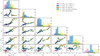 |
Fig. A.1 Fourier phase differences and the amplitude of the first harmonic shown against one another up to the 5th harmonic. The color scheme adopted in Sect. 4.4 is applied to identify specific groups. |
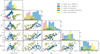 |
Fig. A.2 Fourier amplitude ratios shown against one another up to the 5th harmonic. The color scheme adopted in Sect. 4.4 is applied to identify specific groups. |
Fourier parameters of single-mode Cepheids (excerpt)
Appendix B Stars other than classical Cepheids
In an early phase (mostly between 2011 – 2012), VELOCE targeted candidate type-I Cepheids reported by different photometric surveys, including ASAS (Pojmanski 2002, 2003; Pojmanski & Maciejewski 2004; Pojmanski et al. 2005; Pojmanski & Maciejewski 2005), NSVS (Woźniak et al. 2004), ROTSE (Akerlof et al. 2000), as well as other stars previously classified as Cepheids in order to determine cluster membership (Anderson et al. 2013). A large number of these candidate Cepheids were found not to be Cepheids based on the observed CCFs or, since then, by other variability classification studies (e.g., Johnson 2016). Additionally, a few RR Lyrae stars and type-II Cepheids were observed to fill time during observing runs.
CCFs provide sensitive checks of variable star classifications based on four observational features that allow us to identify bona fide classical Cepheids with only a few observations (Anderson 2013, Sect. 2.4) thanks to the enhanced S/N compared to ordinary spectra and thanks to spectroscopic features. Firstly, classical Cepheids produce noticeable correlation peaks at any phase when cross-correlated with a G2 correlation mask, since their spectral types vary between mid F to early K, cf. Fig. 1. Stars that fail to produce noticeable correlation peaks are thus outside the spectral type range of interest. Cepheid CCFs computed using the G2 masks do not usually exhibit strong rotational broadening, virtually always exhibit a single correlation peak, and virtually never exhibit emission features. However, Cepheid CCFs do generally exhibit phase-dependent displacement in velocity space, phase-dependent line broadening, phase-dependent line asymmetry, and phase-dependent line depth; these parameter are traced by RV, FWHM, BIS, and CCF contrast. Hence, stars that do not exhibit all four types of variations are very likely not classical Cepheids. Johnson (2016).
We have visually inspected the CCFs and their measured parameters of all stars observed for VELOCE. Table B.1 lists the 164 stars that are not classical Cepheids that have been observed as part of VELOCE, including 4 RR Lyrae stars, 12 type-II Cepheids, and 33 (candidate) multi-lined spectroscopic binaries. The table provides qualitative notes on whether the CCF showed a significant correlation peak, whether this peak appeared atypical for Cepheids, whether multiple components were apparent, whether the CCF showed signs of emission features, and whether RV, FWHM, BIS, and Contrast exhibited variability. We also included a brief note concerning the CCF in the hopes that this will be useful in the future. Finally, the table includes the Gaia DR3 source identifier and classifiers assigned by the Gaia DR3 variability analysis (Eyer et al. 2023) and by a literature meta-study of variable stars (Gavras et al. 2023). A detailed reclassification of the stars listed in Tab. B.1 is out of scope of this work. However, we consider that stars can be effectively shown not to be classical Cepheids if they a) exhibit no CCF peaks (NRV), b) exhibit multiple peaks or emission features, or c) do not exhibit all four types of variability despite having been observed more than 4 − 5 times. It is thus possible that a few classical Cepheids remain in Tab. B.1 in case there were only one or two good observations available.
The RV measurements of the stars in Tab. B.1 is published as part of this data release. However, we stress that these RVs have not been vetted, that is, no further quality control was applied. In particular, RVs of SB2 systems need to be considered with caution because it is not always clear that the same CCF peak was measured. Further information on these stars will be published as part of the second data release and is available upon request to the lead author.
Stars previously misclassifled as Cepheid (candidates) observed as part of VELOCE and later found out to not be classical Cepheids (excerpt)
Appendix C VELOCE DR1 data structure
The data published as part of this first VELOCE date release (DR1) are stored in multiple FITS (Flexible Image Transport System) files. Each FITS file contains all the quantities and properties used or derived in the present Paper and/or Paper II dedicated to spectroscopic binaries (Shetye et al. in prep.), and one FITS file is used per stars.
The FITS files are organized using a Header-Data Unit (HDU) list, consisting of a PrimaryHDU and multiple BinTable-HDU16. The HDU contains the header with all the metadata, whereas the BinTableHDU contain the data and results derived in tabular form.
As mentioned above, we applied different parts of our analysis to different stars according to the available data and signal complexity. Hence, the content and number of HDUs vary among the FITS files. However, the file structure consistently follows the different phases of the analysis presented in the two papers.
The most complex file structure is used for stars that underwent all possible stages of the analysis. In this case, the structure of the HDU list is as follows:
- 0.
Primary HDU - Header containing all the metadata (see keys at C.1, C.2, C.3, C.4 and C.5)
- 1.
DATA - BinTableHDU - Table containing the observational data C.6)
- 2.
FIT - BinTableHDU - Coefficients of the model fitted to the RV data (see column names at C.7)
- 3.
RVTF_CLUSTER - BinTableHDU - Results of the template fitting analysis per cluster (see column names at C.8)
- 4.
ZP_CORRECTED - BinTableHDU - Results of the template fitting analysis per observation and zero-point offsets determined for each instrument/source (see column names at C.9)
- 5.
VL_KEPLER - BinTableHDU - Results of the fitted Keplerian orbit after combining VELOCE and literature data (see column names at C.10)
- 6.
VL_CIRCULAR - BinTableHDU - Results of the fitted circular orbit after combining VELOCE and literature data (see column names at C.11)
The first table, DATA - BinTableHDU, is published for all stars for which RVs were measured from CCFs, including stars not modeled and non-Cepheids. The subsequent BinTableHDUs are published only if the corresponding analysis was carried out for a given star. However, the order of the binary tables follows the stream of the analysis so that the order and hierarchy of the HDU are always respected.
All barycentric Julian dates (BJDs) are reported minus 2,400,000 for brevity.
General keys present in the FITS file headers
Additional FITS header keys when a Fourier series model was fitted to VELOCE data
Additional FITS header keys if a Keplerian orbit was fitted to VELOCE data
Additional FITS header keys if both VELOCE and literature data were used to fit a Keplerian orbit using the MCMC method
Additional FITS header keys if both VELOCE and literature data were used to fit a circular orbit using the MCMC method
Content of the first BinTableHDU containing the VELOCE radial velocity measurements
Content of the BinTableHDU containing the model fitted to the RV curve
Per-cluster results of the template fitting analysis
Epoch results of the template fitting analysis
Keplerian fit results based on both VELOCE and literature data using the MCMC method
Circular Keplerian fit results based on both VELOCE and literature data using the MCMC method
References
- Akerlof, C., Amrose, S., Balsano, R., et al. 2000, AJ, 119, 1901 [NASA ADS] [CrossRef] [Google Scholar]
- Anderson, R. I. 2013, PhD thesis, University of Geneva, Switzerland [Google Scholar]
- Anderson, R. I. 2014, A&A, 566, A10 [Google Scholar]
- Anderson, R. I. 2016, MNRAS, 463, 1707 [NASA ADS] [CrossRef] [Google Scholar]
- Anderson, R. I. 2018a, A&A, 611, A7 [Google Scholar]
- Anderson, R. I. 2018b, in The RR Lyrae 2017 Conference. Revival of the Classical Pulsators: from Galactic Structure to Stellar Interior Diagnostics, 6, eds. R. Smolec, K. Kinemuchi, & R. I. Anderson, 193 [Google Scholar]
- Anderson, R. I. 2019, A&A, 623, A146 [NASA ADS] [CrossRef] [EDP Sciences] [Google Scholar]
- Anderson, R. I., Eyer, L., & Mowlavi, N. 2013, MNRAS, 434, 2238 [Google Scholar]
- Anderson, R. I., Sahlmann, J., Holl, B., et al. 2015, ApJ, 804, 144 [CrossRef] [Google Scholar]
- Anderson, R. I., Casertano, S., Riess, A. G., et al. 2016a, ApJS, 226, 18 [NASA ADS] [CrossRef] [Google Scholar]
- Anderson, R. I., Mérand, A., Kervella, P., et al. 2016b, MNRAS, 455, 4231 [NASA ADS] [CrossRef] [Google Scholar]
- Anderson, R. I., Saio, H., Ekström, S., Georgy, C., & Meynet, G. 2016c, A&A, 591, A8 [NASA ADS] [CrossRef] [EDP Sciences] [Google Scholar]
- Antonello, E., & Morelli, P. L. 1996, A&A, 314, 541 [NASA ADS] [Google Scholar]
- Astropy Collaboration (Robitaille, T. P., et al.) 2013, A&A, 558, A33 [NASA ADS] [CrossRef] [EDP Sciences] [Google Scholar]
- Astropy Collaboration (Price-Whelan, A. M., et al.) 2018, AJ, 156, 123 [Google Scholar]
- Baade, W. 1926, Astron. Nachr., 228, 359 [NASA ADS] [CrossRef] [Google Scholar]
- Baranne, A., Queloz, D., Mayor, M., et al. 1996, A&AS, 119, 373 [NASA ADS] [CrossRef] [EDP Sciences] [Google Scholar]
- Baranowski, R., Smolec, R., Dimitrov, W., et al. 2009, MNRAS, 396, 2194 [NASA ADS] [CrossRef] [Google Scholar]
- Barnes, III, T. G., Moffett, T. J., & Slovak, M. H. 1987, ApJS, 65, 307 [NASA ADS] [CrossRef] [Google Scholar]
- Barnes, III, T. G., Moffett, T. J., & Slovak, M. H. 1988, ApJS, 66, 43 [NASA ADS] [CrossRef] [Google Scholar]
- Barnes, III, T. G., Jeffery, E. J., Montemayor, T. J., & Skillen, I. 2005, ApJS, 156, 227 [NASA ADS] [CrossRef] [Google Scholar]
- Becker, W. 1940, ZAp, 19, 289 [NASA ADS] [Google Scholar]
- Belopolsky, A. 1894, Astron. Nachr., 136, 281 [CrossRef] [Google Scholar]
- Belopolsky, A. 1897, ApJ, 6, 393 [NASA ADS] [CrossRef] [Google Scholar]
- Bersier, D. 2002, ApJS, 140, 465 [NASA ADS] [CrossRef] [Google Scholar]
- Bersier, D., Burki, G., Mayor, M., & Duquennoy, A. 1994, A&AS, 108, 25 [NASA ADS] [Google Scholar]
- Blazko, S. 1907, Astron. Nachr., 175, 325 [NASA ADS] [CrossRef] [Google Scholar]
- Borgniet, S., Kervella, P., Nardetto, N., et al. 2019, A&A, 631, A37 [NASA ADS] [CrossRef] [EDP Sciences] [Google Scholar]
- Bouchy, F., Pepe, F., & Queloz, D. 2001, A&A, 374, 733 [NASA ADS] [CrossRef] [EDP Sciences] [Google Scholar]
- Breitfelder, J., Mérand, A., Kervella, P., et al. 2016, A&A, 587, A117 [CrossRef] [EDP Sciences] [Google Scholar]
- Buchler, J. R., Moskalik, P., & Kovacs, G. 1990, ApJ, 351, 617 [NASA ADS] [CrossRef] [Google Scholar]
- Buchschacher, N. & Alesina, F. 2019, in Astronomical Data Analysis Software and Systems XXVI, eds. M. Molinaro, K. Shortridge, & F. Pasian, ASP Conf. Ser., 521, 757 [NASA ADS] [Google Scholar]
- Burki, G., & Mayor, M. 1980, A&A, 91, 115 [NASA ADS] [Google Scholar]
- Burki, G., Mayor, M., & Benz, W. 1982, A&A, 109, 258 [NASA ADS] [Google Scholar]
- Butler, R. P. 1992, ApJ, 394, L25 [NASA ADS] [CrossRef] [Google Scholar]
- Butler, R. P. 1993, ApJ, 415, 323 [NASA ADS] [CrossRef] [Google Scholar]
- Caldwell, J. A. R., Coulson, I. M., Dean, J. F., & Berdnikov, L. N. 2001, J. Astron. Data, 7 [Google Scholar]
- Campbell, W. W. 1899, PASP, 11, 195 [Google Scholar]
- Cardelli, J. A., Clayton, G. C., & Mathis, J. S. 1989, ApJ, 345, 245 [Google Scholar]
- Chazelas, B., Pepe, F., Wildi, F., et al. 2010, SPIE Conf. Ser., 7739, 773947 [NASA ADS] [Google Scholar]
- Chazelas, B., Pepe, F., & Wildi, F. 2012, SPIE Conf. Ser., 8450, 845013 [NASA ADS] [Google Scholar]
- Clementini, G., Ripepi, V., Garofalo, A., et al. 2023, A&A, 674, A18 [NASA ADS] [CrossRef] [EDP Sciences] [Google Scholar]
- Coulson, I. M., & Caldwell, J. A. R. 1985, South Afr. Astron. Observ. Circ., 9, 5 [Google Scholar]
- Coulson, I. M., Caldwell, J. A. R., & Gieren, W. P. 1985, ApJS, 57, 595 [NASA ADS] [CrossRef] [Google Scholar]
- Cretignier, M., Dumusque, X., Hara, N. C., & Pepe, F. 2021, A&A, 653, A43 [NASA ADS] [CrossRef] [EDP Sciences] [Google Scholar]
- Cruz Reyes, M., & Anderson, R. I. 2023, A&A, 672, A85 [NASA ADS] [CrossRef] [EDP Sciences] [Google Scholar]
- Csörnyei, G., Szabados, L., Molnár, L., et al. 2022, MNRAS, 511, 2125 [CrossRef] [Google Scholar]
- de Jong, R. S., Agertz, O., Berbel, A. A., et al. 2019, The Messenger, 175, 3 [NASA ADS] [Google Scholar]
- Derekas, A., Szabó, G. M., Berdnikov, L., et al. 2012, MNRAS, 425, 1312 [NASA ADS] [CrossRef] [Google Scholar]
- Derekas, A., Plachy, E., Molnár, L., et al. 2017, MNRAS, 464, 1553 [NASA ADS] [CrossRef] [Google Scholar]
- Dravins, D., Lindegren, L., Ludwig, H. G., & Madsen, S. 2005, in 13th Cambridge Workshop on Cool Stars, Stellar Systems and the Sun, eds. F. Favata, G. A. J. Hussain, & B. Battrick, ESA Special Publication, 560, 113 [NASA ADS] [Google Scholar]
- Evans, N. R., Berdnikov, L., Lauer, J., et al. 2015a, AJ, 150, 13 [NASA ADS] [CrossRef] [Google Scholar]
- Evans, N. R., Szabó, R., Derekas, A., et al. 2015b, MNRAS, 446, 4008 [CrossRef] [Google Scholar]
- Eyer, L., Audard, M., Holl, B., et al. 2023, A&A, 674, A13 [NASA ADS] [CrossRef] [EDP Sciences] [Google Scholar]
- Fadeyev, Y. A. 2014, Astron. Lett., 40, 301 [NASA ADS] [CrossRef] [Google Scholar]
- Gaia Collaboration (Prusti, T., et al.) 2016, A&A, 595, A1 [NASA ADS] [CrossRef] [EDP Sciences] [Google Scholar]
- Gaia Collaboration (Vallenari, A., et al.) 2023, A&A, 674, A1 [NASA ADS] [CrossRef] [EDP Sciences] [Google Scholar]
- Gallenne, A., Kervella, P., Evans, N. R., et al. 2018, ApJ, 867, 121 [Google Scholar]
- Gallenne, A., Kervella, P., Borgniet, S., et al. 2019, A&A, 622, A164 [NASA ADS] [CrossRef] [EDP Sciences] [Google Scholar]
- Gavras, P., Rimoldini, L., Nienartowicz, K., et al. 2023, A&A, 674, A22 [NASA ADS] [CrossRef] [EDP Sciences] [Google Scholar]
- Gieren, W. P. 1981, ApJS, 46, 287 [NASA ADS] [CrossRef] [Google Scholar]
- Gieren, W. P. 1985, ApJ, 295, 507 [NASA ADS] [CrossRef] [Google Scholar]
- Gieren, W. P., Matthews, J. M., Moffett, T. J., et al. 1989, AJ, 98, 1672 [NASA ADS] [CrossRef] [Google Scholar]
- Gieren, W., Storm, J., Konorski, P., et al. 2018, A&A, 620, A99 [NASA ADS] [CrossRef] [EDP Sciences] [Google Scholar]
- Gorynya, N. A. 1998, Inform. Bull. Variable Stars, 4636, 1 [NASA ADS] [Google Scholar]
- Gorynya, N. A., Irsmambetova, T. R., Rastorgouev, A. S., & Samus, N. N. 1992, Sov. Astron. Lett., 18, 316 [NASA ADS] [Google Scholar]
- Gorynya, N. A., Rastorguev, A. S., & Samus, N. N. 1996, Astron. Lett., 22, 33 [NASA ADS] [Google Scholar]
- Gorynya, N. A., Samus’, N. N., Sachkov, M. E., et al. 1998, Astron. Lett., 24, 815 [Google Scholar]
- Groenewegen, M. A. T. 2018, A&A, 619, A8 [NASA ADS] [CrossRef] [EDP Sciences] [Google Scholar]
- Hatzes, A. P., & Cochran, W. D. 2000, AJ, 120, 979 [CrossRef] [Google Scholar]
- Hertzsprung, E. 1926, Bull. Astron. Inst. Netherlands, 3, 115 [Google Scholar]
- Hocdé, V., Nardetto, N., Borgniet, S., et al. 2020, A&A, 641, A74 [EDP Sciences] [Google Scholar]
- Imbert, M. 1984, A&AS, 58, 529 [NASA ADS] [Google Scholar]
- Imbert, M. 1999, A&AS, 140, 79 [NASA ADS] [CrossRef] [EDP Sciences] [Google Scholar]
- Jin, S., Trager, S. C., Dalton, G. B., et al. 2024, MNRAS, 530, 2688 [NASA ADS] [CrossRef] [Google Scholar]
- Johnson, J. 2016, JAAVSO, 44, 81 [NASA ADS] [Google Scholar]
- Joy, A. H. 1937, ApJ, 86, 363 [NASA ADS] [CrossRef] [Google Scholar]
- Katz, D., Sartoretti, P., Guerrier, A., et al. 2023, A&A, 674, A5 [NASA ADS] [CrossRef] [EDP Sciences] [Google Scholar]
- Kervella, P., Trahin, B., Bond, H. E., et al. 2017, A&A, 600, A127 [NASA ADS] [CrossRef] [EDP Sciences] [Google Scholar]
- Khan, S., Anderson, R. I., Miglio, A., Mosser, B., & Elsworth, Y. P. 2023, A&A, 680, A105 [NASA ADS] [CrossRef] [EDP Sciences] [Google Scholar]
- Kienzle, F., Moskalik, P., Bersier, D., & Pont, F. 1999, A&A, 341, 818 [NASA ADS] [Google Scholar]
- Kiss, L. L. 1998, MNRAS, 297, 825 [NASA ADS] [CrossRef] [Google Scholar]
- Klagyivik, P., & Szabados, L. 2009, A&A, 504, 959 [NASA ADS] [CrossRef] [EDP Sciences] [Google Scholar]
- Kovacs, G., Kisvarsanyi, E. G., & Buchler, J. R. 1990, ApJ, 351, 606 [NASA ADS] [CrossRef] [Google Scholar]
- Kovtyukh, V. V., Andrievsky, S. M., Luck, R. E., & Gorlova, N. I. 2003, A&A, 401, 661 [NASA ADS] [CrossRef] [EDP Sciences] [Google Scholar]
- Lindemann, F. A. 1918, MNRAS, 78, 639 [NASA ADS] [CrossRef] [Google Scholar]
- Lindegren, L., & Dravins, D. 2003, A&A, 401, 1185 [NASA ADS] [CrossRef] [EDP Sciences] [Google Scholar]
- Lindegren, L., Bastian, U., Biermann, M., et al. 2021, A&A, 649, A4 [EDP Sciences] [Google Scholar]
- Lloyd Evans, T. 1980, South Afr. Astron. Observ. Circ., 1, 257 [Google Scholar]
- Lo Curto, G., Pepe, F., Avila, G., et al. 2015, The Messenger, 162, 9 [NASA ADS] [Google Scholar]
- Luri, X., Brown, A. G. A., Sarro, L. M., et al. 2018, A&A, 616, A9 [NASA ADS] [CrossRef] [EDP Sciences] [Google Scholar]
- Madore, B. F. 1982, ApJ, 253, 575 [NASA ADS] [CrossRef] [Google Scholar]
- Majewski, S. R., Schiavon, R. P., Frinchaboy, P. M., et al. 2017, AJ, 154, 94 [NASA ADS] [CrossRef] [Google Scholar]
- Martin, D. V., Triaud, A. H. M. J., Udry, S., et al. 2019, A&A, 624, A68 [NASA ADS] [CrossRef] [EDP Sciences] [Google Scholar]
- Mathias, P., Gillet, D., Fokin, A. B., et al. 2006, A&A, 457, 575 [CrossRef] [EDP Sciences] [Google Scholar]
- Mayor, M., & Queloz, D. 1995, Nature, 378, 355 [Google Scholar]
- Metzger, M. R., Caldwell, J. A. R., McCarthy, J. K., & Schechter, P. J. 1991, ApJS, 76, 803 [NASA ADS] [CrossRef] [Google Scholar]
- Metzger, M. R., Caldwell, J. A. R., & Schechter, P. L. 1992, AJ, 103, 529 [NASA ADS] [CrossRef] [Google Scholar]
- Miller, C. L., Neilson, H. R., Evans, N. R., Engle, S. G., & Guinan, E. 2020, ApJ, 896, 128 [Google Scholar]
- Molnár, L., & Szabados, L. 2014, MNRAS, 442, 3222 [Google Scholar]
- Molnár, L., Derekas, A., Szabó, R., et al. 2017, MNRAS, 466, 4009 [Google Scholar]
- Moskalik, P., & Kolaczkowski, Z. 2009, MNRAS, 394, 1649 [Google Scholar]
- Nardetto, N., Mourard, D., Kervella, P., et al. 2006, A&A, 453, 309 [NASA ADS] [CrossRef] [EDP Sciences] [Google Scholar]
- Nardetto, N., Mourard, D., Mathias, P., Fokin, A., & Gillet, D. 2007, A&A, 471, 661 [NASA ADS] [CrossRef] [EDP Sciences] [Google Scholar]
- Nardetto, N., Stoekl, A., Bersier, D., & Barnes, T. G. 2008, A&A, 489, 1255 [NASA ADS] [CrossRef] [EDP Sciences] [Google Scholar]
- Nardetto, N., Poretti, E., Rainer, M., et al. 2017, A&A, 597, A73 [CrossRef] [EDP Sciences] [Google Scholar]
- Netzel, H., Anderson, R. I., & Viviani, G. 2024, A&A, accepted [arXiv:2403.13796] [Google Scholar]
- Pasquini, L., Melo, C., Chavero, C., et al. 2011, A&A, 526, A127 [NASA ADS] [CrossRef] [EDP Sciences] [Google Scholar]
- Pedregosa, F., Varoquaux, G., Gramfort, A., et al. 2011, J. Mach. Learn. Res., 12, 2825 [Google Scholar]
- Pepe, F., Mayor, M., Galland, F., et al. 2002, A&A, 388, 632 [NASA ADS] [CrossRef] [EDP Sciences] [Google Scholar]
- Pepe, F., Bouchy, F., Queloz, D., & Mayor, M. 2003, in Scientific Frontiers in Research on Extrasolar Planets, eds. D., Deming & S. Seager, ASP Conf. Ser., 294, 39 [NASA ADS] [Google Scholar]
- Pietrukowicz, P., Soszyński, I., & Udalski, A. 2021, Acta Astron., 71, 205 [NASA ADS] [Google Scholar]
- Plachy, E., Pál, A., Bódi, A., et al. 2021, ApJS, 253, 11 [NASA ADS] [CrossRef] [Google Scholar]
- Pojmanski, G. 2002, Acta Astron., 52, 397 [NASA ADS] [Google Scholar]
- Pojmanski, G. 2003, Acta Astron., 53, 341 [NASA ADS] [Google Scholar]
- Pojmanski, G., & Maciejewski, G. 2004, Acta Astron., 54, 153 [CrossRef] [Google Scholar]
- Pojmanski, G., & Maciejewski, G. 2005, Acta Astron., 55, 97 [NASA ADS] [Google Scholar]
- Pojmanski, G., Pilecki, B., & Szczygiel, D. 2005, Acta Astron., 55, 275 [NASA ADS] [Google Scholar]
- Pont, F., Burki, G., & Mayor, M. 1994, A&AS, 105, 165 [NASA ADS] [Google Scholar]
- Pont, F., Queloz, D., Bratschi, P., & Mayor, M. 1997, A&A, 318, 416 [NASA ADS] [Google Scholar]
- Poretti, E., Le Borgne, J. F., Rainer, M., et al. 2015, MNRAS, 454, 849 [NASA ADS] [CrossRef] [Google Scholar]
- Queloz, D., Mayor, M., Udry, S., et al. 2001, The Messenger, 105, 1 [NASA ADS] [Google Scholar]
- Raskin, G., van Winckel, H., Hensberge, H., et al. 2011, A&A, 526, A69 [CrossRef] [EDP Sciences] [Google Scholar]
- Rathour, R. S., Smolec, R., & Netzel, H. 2021, MNRAS, 505, 5412 [NASA ADS] [CrossRef] [Google Scholar]
- Ricker, G. R., Winn, J. N., Vanderspek, R., et al. 2015, J. Astron. Telescopes Instrum. Syst., 1, 014003 [Google Scholar]
- Riess, A. G., Casertano, S., Yuan, W., et al. 2018a, ApJ, 855, 136 [CrossRef] [Google Scholar]
- Riess, A. G., Casertano, S., Yuan, W., et al. 2018b, ApJ, 861, 126 [CrossRef] [Google Scholar]
- Riess, A. G., Casertano, S., Yuan, W., et al. 2021, ApJ, 908, L6 [NASA ADS] [CrossRef] [Google Scholar]
- Riess, A. G., Yuan, W., Macri, L. M., et al. 2022, ApJ, 934, L7 [NASA ADS] [CrossRef] [Google Scholar]
- Ripepi, V., Clementini, G., Molinaro, R., et al. 2023, A&A, 674, A17 [NASA ADS] [CrossRef] [EDP Sciences] [Google Scholar]
- Sartoretti, P., Marchal, O., Babusiaux, C., et al. 2023, A&A, 674, A6 [NASA ADS] [CrossRef] [EDP Sciences] [Google Scholar]
- Ségransan, D., Udry, S., Mayor, M., et al. 2010, A&A, 511, A45 [NASA ADS] [CrossRef] [EDP Sciences] [Google Scholar]
- Simon, N. R., & Lee, A. S. 1981, ApJ, 248, 291 [NASA ADS] [CrossRef] [Google Scholar]
- Smolec, R. 2017, MNRAS, 468, 4299 [NASA ADS] [CrossRef] [Google Scholar]
- Smolec, R., & Śniegowska, M. 2016, MNRAS, 458, 3561 [NASA ADS] [CrossRef] [Google Scholar]
- Smolec, R., Ziółkowska, O., Ochalik, M., & Sniegowska, M. 2023, MNRAS, 519, 4010 [NASA ADS] [CrossRef] [Google Scholar]
- Soszyński, I., Udalski, A., Szymanski, M. K., et al. 2015, Acta Astron., 65, 329 [Google Scholar]
- Sterken, C. 2005, in The Light-Time Effect in Astrophysics: Causes and cures of the O-C diagram, ed. C. Sterken, ASP Conf. Ser., 335, 3 [NASA ADS] [Google Scholar]
- Stibbs, D. W. N. 1955, MNRAS, 115, 363 [NASA ADS] [Google Scholar]
- Storm, J., Carney, B. W., Gieren, W. P., et al. 2004, A&A, 415, 531 [NASA ADS] [CrossRef] [EDP Sciences] [Google Scholar]
- Storm, J., Gieren, W., Fouqué, P., et al. 2011, A&A, 534, A94 [CrossRef] [EDP Sciences] [Google Scholar]
- Struve, O. 1945, ApJ, 102, 232 [NASA ADS] [CrossRef] [Google Scholar]
- Süveges, M., & Anderson, R. I. 2018a, MNRAS, 478, 1425 [CrossRef] [Google Scholar]
- Süveges, M., & Anderson, R. I. 2018b, A&A, 610, A86 [NASA ADS] [CrossRef] [EDP Sciences] [Google Scholar]
- Szabados, L. 1989, Commmun. Konkoly Observ. Hungary, 94, 1 [NASA ADS] [Google Scholar]
- Szabados, L., Derekas, A., Kiss, L. L., et al. 2013, MNRAS, 430, 2018 [NASA ADS] [CrossRef] [Google Scholar]
- Taylor, M. 2024, arXiv e-prints [arXiv:2401.01156] [Google Scholar]
- Tiercy, G. 1928, Publ. Observ. Geneve Ser. A, 2, 5 [NASA ADS] [Google Scholar]
- Tiercy, G., Abetti, G., & Colacevich, A. 1928, Osservazioni memorie Osservatorio astrofisico Arcetri, 45, 1 [NASA ADS] [Google Scholar]
- Tokovinin, A. 2014, AJ, 147, 86 [Google Scholar]
- Torres, G. 2023, MNRAS, 526, 2510 [NASA ADS] [CrossRef] [Google Scholar]
- Trahin, B., Breuval, L., Kervella, P., et al. 2021, A&A, 656, A102 [NASA ADS] [CrossRef] [EDP Sciences] [Google Scholar]
- Turner, D. G., Savoy, J., Derrah, J., Abdel-Sabour Abdel-Latif, M., & Berdnikov, L. N. 2005, PASP, 117, 207 [CrossRef] [Google Scholar]
- Turner, D. G., Abdel-Sabour Abdel-Latif, M., & Berdnikov, L. N. 2006, PASP, 118, 410 [Google Scholar]
- Udry, S., Mayor, M., Maurice, E., et al. 1999a, in IAU Colloq. 170: Precise Stellar Radial Velocities, eds. J. B. Hearnshaw, & C. D. Scarfe, ASP Conf. Ser., 185, 383 [NASA ADS] [Google Scholar]
- Udry, S., Mayor, M., & Queloz, D. 1999b, in IAU Colloq. 170: Precise Stellar Radial Velocities, eds. J. B. Hearnshaw, & C. D. Scarfe, ASP Conf. Ser., 185, 367 [NASA ADS] [Google Scholar]
- Usenko, I. A., Kniazev, A. Y., Berdnikov, L. N., Fokin, A. B., & Kravtsov, V. V. 2014, Astron. Lett., 40, 435 [NASA ADS] [CrossRef] [Google Scholar]
- Van Malle, M. 2016, PhD thesis, iD: unige:88749 [Google Scholar]
- Wallerstein, G., Anderson, R. I., Farrell, E. M., et al. 2019, PASP, 131, 094203 [CrossRef] [Google Scholar]
- Wesselink, A. J. 1946, Bull. Astron. Inst. Netherlands, 10, 91 [Google Scholar]
- Wilson, T. D., Carter, M. W., Barnes, III, T. G., van Citters, Jr., G. W., & Moffett, T. J. 1989, ApJS, 69, 951 [NASA ADS] [CrossRef] [Google Scholar]
- Woźniak, P. R., Vestrand, W. T., Akerlof, C. W., et al. 2004, AJ, 127, 2436 [Google Scholar]
In particular the work by Georges Tiercy at Geneva Observatory in the 1920s deserves a special mention as it has not received the attention it deserves, likely because the texts were written in French and are not yet fully accessible. Further work to render the exceptional light and RV curves of Galactic Cepheids measured by Tiercy would be warranted from a historical perspective.
BG Vel, IT Car, MY Pup, U Vul, V1334 Cyg, V5567 Sgr, VY Per, VZ Pup, and W Sgr.
Excluding binaries HD 154417, HD 168009, and HD 42807.
We previously reported this finding in September 2022 and April 2023 at the RR Lyrae and Cepheids conference in La Palma, Spain and at IAU Symposium 376 in Budapest, Hungary.
Variable periods are discussed in Sect. 5.3 below. Suffice it here to mention that period fluctuations contribute to the rms of the RV curve, in particular near the steepest parts of the RV curve, since our baseline Fourier series model assumes a fixed Ppuls. However, this applies primarily to fast, non-linear period changes, since secular (linear) period changes are generally too slow (mostly <10 s yr−1) to significantly change P over the VELOCE baseline.
Klagyivik & Szabados (2009, their Fig. 12) considered the related, albeit less readily interpreted, quantity ARV × P as a function of log P to argue for a division of fundamental mode Cepheids into short- and long-period groups at a period of 10.47 days (log P = 1.02). In their search for spectroscopic binaries or identifications of pulsation modes, Klagyivik et al. came to the conclusion that light-to-RV amplitude ratios were not always reliable indicators of pulsation modes or the presence of companions, although no clear physical reason could be offered. No distinction among the long-period Cepheids was made by the authors.
Details of the SB1 nature of Cepheids in the VELOCE sample are provided in Paper II.
While Fig. 22 is useful for this specific comparison, we stress that the sample of Cepheids shown here was not selected to provide a meaningful test of the LL calibration, and that it contains stars whose astrometry or photometry may not be suitable to calibrate the LL, e.g., due to blending or poor astrometry, or whose parallaxes should not be inverted to determine distance (cf. Luri et al. 2018). Two significant outliers with visual companions were removed, however: SY Nor, whose visual companion is seen in Coralie guiding camera, and SV Per, whose companion is barely resolved by HST/WFC3 spatial scanning observations (Riess et al. 2018b).
Only epochs with |Δυr| ≤ 4 km s−1 as well as σ(Δυr) < 0.2 km s−1 were considered for most newer and very precise data sets. Data from Gieren (1985); Barnes et al. (1987); Wilson et al. (1989); Caldwell et al. (2001); Coulson et al. (1985); Coulson & Caldwell (1985); Gieren (1981); Metzger et al. (1992); Kiss (1998); Joy (1937); Stibbs (1955); Struve (1945) and Gaia DR3 were considered if σ(Δυr) < 3.0 km s−1.
Ncyc,E is usually written simply as E in the literature (Sterken 2005). We here adopt Ncyc,E to distinguish this from our pulsation ephemerides epoch E used in Sect. 3.1 and to highlight that this refers to a number of pulsation cycles.
An erroneous period would show as a straight line in Fig. 16.
These corner plots were inspired by Taylor (2024).
A detailed description of this kind of files and how to handle them is given in the astropy.io.fits library documentation at https://docs.astropy.org/en/stable/io/fits/index.html
All Tables
Stars previously misclassifled as Cepheid (candidates) observed as part of VELOCE and later found out to not be classical Cepheids (excerpt)
Additional FITS header keys when a Fourier series model was fitted to VELOCE data
Additional FITS header keys if both VELOCE and literature data were used to fit a Keplerian orbit using the MCMC method
Additional FITS header keys if both VELOCE and literature data were used to fit a circular orbit using the MCMC method
Content of the first BinTableHDU containing the VELOCE radial velocity measurements
Keplerian fit results based on both VELOCE and literature data using the MCMC method
Circular Keplerian fit results based on both VELOCE and literature data using the MCMC method
All Figures
|
Fig. 1 Example CCFs for four pulsating stars as labeled. The color traces the pulsation phase. KN Cen is a long-period, high-amplitude type-I Cepheid. The others are prototypes of their respective pulsating star classes. CCF shape variations follow a characteristic pattern for type-I Cepheids. RR Lyrae stars are hotter and feature shallower CCFs with very large amplitudes and line asymmetry, whereas W Virginis stars can exhibit signatures of shock phenomena at specific phases, including blue-shifted emission features and line splitting. |
| In the text | |
|
Fig. 2 Short-burst (42 and 34 min) RV time series of the 20 days Cepheid RZ Vel near minimum RV collected to test the momentaneous precision of Coralie07 and Coralie14. Both panels show the measured RV minus the mean of the sequence. Shaded areas illustrate the dispersion of the sequences. Average S/N on the 60th echelle order are labeled for reference. Note the improved precision of Coralie14 over Coralie07. Top panel: Coralie07 observations taken on 22 June 2011. Note the change of exposure time (vertical dotted line) that affects both precision and uncertainties estimated by the pipeline. Bottom panel: Coralie14 observations collected on 5 March 2018. |
| In the text | |
|
Fig. 3 RV drift corrections determined from pressure variations (Eq. (1)) against the corrections determined via simultaneous drift corrections based on interlaced ThAr spectra. The discretization of the results is due to the single-decimal precision with which the atmospheric pressure is recorded in the FITS headers. The black dotted line shows the equality Δυ(ΔP) = ΔυTh, whereas the blue, red, and green lines are the best linear fits to the Coralie07, Coralie14, and combined Coralie distributions, as quantified in the legend. |
| In the text | |
|
Fig. 4 Sky coverage of VELOCE targets in sky coordinates (left) and Galactic coordinates (right). Bona fide Cepheids are shown as red filled circles, stars that are not classical Cepheids are shown as open circles. |
| In the text | |
|
Fig. 5 Mean per epoch RV uncertainty of bona fide Cepheids with at least 9 observations as a function of the mean Gaia DR3 G-band magnitude, cf. Table A.1. Coralie uncertainties (green points) are estimated differently from Hermes uncertainties, cf. Sect. 2.3, and are limited by photon noise. Hermes uncertainties (red points) are overestimated for G ≲ 10 mag. The brightest star, Polaris, is missing due to a lack of Gaia photometry; the faintest target is GL Cyg. X Sgr is excluded from the plot due to significant line shape distortions (Mathias et al. 2006; Anderson 2013) that complicate uncertainty estimation. |
| In the text | |
|
Fig. 6 Distribution of pulsation periods of Cepheids in VELOCE. The red histograms shows all classical Cepheids, while the blue histogram shows the stars used to determine instrumental zero-points, cf. Sects. 5.2 and 5.4. |
| In the text | |
|
Fig. 7 Distribution of the number of observations per Cepheid. The red histogram shows the available number of observations (Nobs) of all Cepheids in VELOCE. The blue histogram shows the number of measurements used to fit Cepheid RV curves (Nobs,fitted). The bin edges are identical for both histograms and logarithmically spaced. The first 8 bins of the red histogram are shown individually to improve readability; a threshold of at least 9 observations was used to fit pulsational models (Sect. 3.3.1). Differences between the blue and red histograms at Nobs > 8 arise due to data selection for model fitting (e.g., in the case of binaries, Sect. 3.3) or additional signals preventing a reasonable fit (Sect. 4.3). The legend summarizes the median and total number of VELOCE observations per group. |
| In the text | |
|
Fig. 8 Distributions of the number ratios of Cepheids in VELOCE to those in Gaia as a function of magnitude (left) and Ppuls (right). The comparison is limited to 245 VELOCE Cepheids for which G-band magnitudes are available and to |
| In the text | |
|
Fig. 9 Illustration of the automated model selection procedure. Up to twenty harmonics were computed in a brute force approach, depending on data availability. The statistical significance of increasing the model’s complexity was assessed using both F-test (p < 0.05) and BIC (ΔBIC < 0) criteria. Violations of these criteria were accepted if the two subsequent, more complex, models both indicated significant fit improvements. The improvement χ2/NDOF of the fit is shown in green. |
| In the text | |
|
Fig. 10 Number of Fourier series harmonics (NFS) used vs. number of observations available (Nobs). The black dash-dotted line shows the maximum number of harmonics that can be fitted for a given number of observations, Nobs = 2 • NFS + 1. The red dotted lines and shaded area show increasing numbers of degrees of freedom (up to ND0F = 10). |
| In the text | |
|
Fig. 11 Fourier parameters for 219 Cepheids in VELOCE as a function of log P up to the 7th harmonic. Some phase differences were shifted by ±2π for clarity. Errorbars are plotted for all stars but are usually smaller than the symbols. The number of harmonics fitted is color coded from light yellow (NFS = 2) to dark red (NFS = 10 is darkest shade for clarity). Overtone Cepheids are clearly apparent at low amplitudes and short periods. Excess dispersion in ϕ51 and ϕ61 near 1.0 ≲ log P ≲ 1.2 is a consequence of the well-known resonance between the fundamental mode and the second overtone (Simon & Lee 1981 ; Buchler et al. 1990; Antonello & Morelli 1996). These results are further illustrated in Appendix A.1. |
| In the text | |
|
Fig. 12 Hertzsprung progression illustrated by the model RV curves of 208 fitted Cepheids (11 low-amplitude stars were removed for clarity). Cepheids are offset in the vertical direction according to their log Ppuls. Errorbars near the top show the constant velocity scale. Vertical dotted lines indicate ϕ = 0, the phase of minimum radius. Left panel, left column: Cepheids classified as first overtone pulsators in Gaia DR3. Left panel, right column: Cepheids classified as fundamental mode pulsators in Gaia DR3. Outliers with particularly small amplitudes are not shown for clarity (cf. Sect. 4.4). The shortest-period FU Cepheids is BP Cir. Right panels: close up view in the period range 9–18 days. Stars with double-peaked bump features are shown in blue on the right, stars with single-peaked bumps on the left in black. Names are color coded accordingly. Outliers Z Lac, CH Cas, and Y Oph are not shown for clarity. The double-peaked bump appears in 31/61 ≈ 50% of VELOCE Cepheids and may be a ubiquitous feature of Cepheid RV curves that requires very high precision and extremely dense phase sampling for detection. |
| In the text | |
|
Fig. 13 VELOCE data and fit to XX Car, which exhibits a double-bumped descending RV branch. Only Coralie14 observations were used in this Fourier series fit employing 13 harmonics. The two peaks are clearly sampled. The data quality is sufficient to show the shortcoming of the Fourier series fit in reproducing the two bumps whose slopes are slightly less steep than implied by the fit to the overall RV curve. |
| In the text | |
|
Fig. 14 Cepheids exhibiting double bumps on the declining RV curve part stand out in the ϕ41 vs. R21 diagram as a “connecting band” between two otherwise parallel sequences. In ϕ41 − ϕ31 vs. R21, double bump Cepheids also follow a significantly different trend. Plotting these parameters could serve to identify double bumps Cepheids in a quantitative manner rather than by visual inspection of the fits. |
| In the text | |
|
Fig. 15 Normalized χ2/NDOF of VELOCE Fourier series fits vs. the median uncertainty of the RV measurements for 151 non-SB1 Cepheids. The rapid increase of χ2/NDOF for precise measurements with typical uncertainties better than 20–40 m s−1 shows the existence of additional signals that are not reproduced by Fourier series models with constant Ppuls. The three longest-period Cepheids in the sample, GS Lup, SV Vul, and S Vul are labeled and highlighted. |
| In the text | |
|
Fig. 16 Phase shifts vs. observation date for R Cru determined by template fitting. The long-term change in Δϕ is the signature of secular period change (cf. Sect. 5.3), whereas an oscillatory pattern among the VELOCE data is also clearly apparent. R Cru is the Cepheid with the shortest known orbital period in the MW, Porb = 237.6 days (cf. Paper II). |
| In the text | |
|
Fig. 17 RV curve integrals (=ΔR/p) vs. log P determined from the VELOCE best fit models. Short-period Cepheids (Ppuls < 10 days) are separated into low- and high-amplitude stars using a peak-to-peak RV threshold of 20 km s−1 and color coded in purple (≤ 20 km s−1) and blue (>20 km s−1). Long-period (P > 10d) FU Cepheids exhibit a strikingly (~5.6–6.6×) steeper trend than short-period Cepheids. We introduce an ad hoc distinction among three sequences for P > 10 d FU Cepheids into stars exhibiting large (yellow), intermediate (green), and small (orange) radius variations. The right panel shows a close-up view to more easily distinguish among short-period Cepheids, where a large number of Cepheids are found between the well-defined envelopes made up of FU and FO Cepheids, respectively. Stars near the edges are labeled to facilitate identification. |
| In the text | |
|
Fig. 18 Double-logarithmic plot of ΔR/p vs. Ppuls. All stars on the low-ΔR/p sequence are labeled. Color coding as in Fig. 17. |
| In the text | |
|
Fig. 19 Ratio of amplitudes between 4th and 2nd harmonic vs. ϕ41. Low ΔR/p stars have consistently low R42 more similar to short-period Cepheids, while high ΔR/p stars exhibit a very large range in R42 near 3.5 ≲ ϕ41 ≲ 4.5. |
| In the text | |
|
Fig. 20 Iron abundances compiled by Groenewegen (2018) for long-period Cepheids on the low- (orange), intermediate- (green), and high-ΔR/p (yellow) sequences introduced in Fig. 17. The binned histograms are superposed by KDE-smoothed distributions. No clear difference in metallicity is apparent between the three groups. |
| In the text | |
|
Fig. 21 Color magnitude diagram of VELOCE stars based on V- and K-band magnitudes and color excesses compiled by Groenewegen (2018), de-reddened using the Cardelli et al. (1989) reddening law. Color coding distinguishes between long-period Cepheids (Ppuls > 10 days) with low (orange), intermediate (green), and high (yellow) ΔR/p, as well as short-period (Ppuls < 10 days) high-RV amplitude (blue) and low-RV (purple). |
| In the text | |
|
Fig. 22 Comparison of the stars belonging to the five subgroups in Fig. 17 shown in relation to the FU Cepheid MW Leavitt law calibrated using cluster Cepheids (Cruz Reyes & Anderson 2023, black solid line) and the reddening-free Wesenheit magnitude WG. Low-ΔR Cepheids are shown in orange and are not systematic outliers from the LL. The most significant outliers are Y Oph (7.1σ from the LL, ⟨mG⟩ = 5.5 mag) and S Vul (3.9σ, ⟨mG⟩ = 6.7 mag). The limitations of this comparison are described in the text. |
| In the text | |
|
Fig. 23 Example template fits to literature data of stars with VELOCE RVs. Two parameters are fitted: the mean offset Δυγ and the phase offset Δϕ. The RV curve shapes and amplitudes are fixed by the VELOCE best fit models. From left to right: FN Aql observations by Barnes et al. (2005) closely fit to the VELOCE template; AX Cir observations by Lloyd Evans (1980) are sufficient to achieve a good template fit; BZ Cyg observations by Gorynya et al. (1992) show some scatter but the template fit is reliable thanks to dense phase sampling; even just seven VELOCE observations of R Mus allow for a precise template fit. |
| In the text | |
|
Fig. 24 Example of temporal data clustering based on KDE. The solid green lines indicate the kernel density estimate, and data are clustered temporally according to local KDE minima. From left to right: observations of S Cru by Gieren (1981) are insufficiently sampled for temporal clustering and used all together; observations of FF Aql by Gorynya et al. (1998) can and must be clustered during later epochs due to significant orbital motion; observations of KN Cen from VELOCE can be separated into several well-sampled data clusters; S Vul observations in VELOCE were separated into data clusters, although not all clusters could be used due to insufficient data points and rapid period fluctuations. |
| In the text | |
|
Fig. 25 Determination of RV zero-points as a function of time for different references. From top to bottom: Gorynya et al. (1998), the previously largest data set of classical Cepheid RV time series; Kienzle et al. (1999); Borgniet et al. (2019). Only stars with VELOCE observations are used to determine zero-points. Horizontal errorbars indicate the time span of the measurements. A solid red line shows an unweighted linear fit to investigate temporal trends; the dotted black line shows the median with its standard error as a grey shaded region. |
| In the text | |
|
Fig. 26 RV zero-point stability for the three instruments distinguished here, Coralie07, Coralie14, and Hermes relative to the overall VELOCE zero-point set by the combined dataset of all Cepheids, which includes stars observed with both Coralie versions, as well as with Hermes and Coralie. The vertical scale and color scheme is identical to Fig. 25. Horizontal errorbars indicate the time span of the measurements. Outliers from the median are mostly due to imperfect template fits or low-amplitude signals mimicking temporal variations in υγ. The Hermes zero-point change due to the intervention in 2018 is visible near BJD 58300, cf. Table 1. |
| In the text | |
|
Fig. 27 Double-logarithmic plot of linear period changes, |
| In the text | |
|
Fig. 28 Example VELOCE model template fits to Gaia RVs. Top row: the full set of Gaia RVs for SS CMa is fitted at once (left) or split into two epoch (center and right). gaiadr3.gaia_source does not provide the template parameters for SS CMa despite Gaia RVs being available in gaiadr3.vari_epoch_rv. Bottom row: stars whose Gaia RVs were determined using different temperatures (from left to right: TX Cyg (4250K), WX Pup (5250K), AV Cir (6250K)). VELOCE uses a correlation mask created to match spectral type G2. |
| In the text | |
|
Fig. 29 Comparison of Gaia DR3 parameter average_rv from table gaiadr3.vari_Cepheid, υγ,GDR3, to the pulsation-averaged velocity derived by template fitting of the Gaia DR3 RV time series, |
| In the text | |
|
Fig. 30 Differences between |
| In the text | |
|
Fig. 31 Difference Δυγ = υγ,GDR3−υγVELOCE between parameter average_rv from gaiadr3.vari_cepheid and υγ from VELOCE for 71 well-behaved non-SB1 Cepheids as a function of the Gaia correlation template parameters and the number of Gaia time series observations, num_clean_epochs_rv. Orange points highlight the 33 Cepheids whose Gaia RVs were measured using the most suitable template parameter range 5000 ≤Teff ≤ 6500, log g ≤ 2, and −0.75 ≤ [Fe/H] ≤ 0.75. The green point in the right-most panel is RW Cas, for which the template parameters are not known. Trends appear among all template parameters, with cooler templates or higher-log g templates yielding larger positive offset. RVs measured using adequate template parameters show significantly improved scatter. |
| In the text | |
|
Fig. 32 Ratio of the peak-to-peak RV amplitudes from Gaia DR3 (peak_to_peak_rv from table gaiadr3.vari_cepheid) to the VELOCE peak-to-peak RV amplitudes as a function of the template parameters, analogous to Fig. 31. The amplitude ratios exhibit large scatter. However, no clear trends emerge. |
| In the text | |
|
Fig. 33 υγ (left) and peak-to-peak RV amplitude (right) determined by Gaia SOS compared to VELOCE as a function of logarithmic pulsation period. υγ,GDR3 and Ap2p,GDR3 are the values published in table gaiadr3.vari_cepheid as parameters average_rv and peak_to_peak_rv, respectively. Orange points highlight Cepheids for which Gaia used the most adequate template parameters. Blue points show measurements processed using template parameters outside this range. Blue and orange solid lines show linear fits to the respective points; green solid lines show linear fits to the combined data sets. At log P = 1, we find Δυγ = 0.51 ± 0.13 km s−1, and a slight trend of 1.03 ± 0.29 km s−1/log P for the orange points. The blue points exhibit a much more significant offset of 1.6 ± 0.2 km s−1 and trend 1.69 ± 0.44 km s−1 / log P. Peak-to-peak amplitudes are generally consistent with a dispersion of approximately 16% and do not exhibit a trend with log P. |
| In the text | |
|
Fig. A.1 Fourier phase differences and the amplitude of the first harmonic shown against one another up to the 5th harmonic. The color scheme adopted in Sect. 4.4 is applied to identify specific groups. |
| In the text | |
|
Fig. A.2 Fourier amplitude ratios shown against one another up to the 5th harmonic. The color scheme adopted in Sect. 4.4 is applied to identify specific groups. |
| In the text | |
Current usage metrics show cumulative count of Article Views (full-text article views including HTML views, PDF and ePub downloads, according to the available data) and Abstracts Views on Vision4Press platform.
Data correspond to usage on the plateform after 2015. The current usage metrics is available 48-96 hours after online publication and is updated daily on week days.
Initial download of the metrics may take a while.