| Issue |
A&A
Volume 694, February 2025
|
|
|---|---|---|
| Article Number | A273 | |
| Number of page(s) | 15 | |
| Section | Stellar structure and evolution | |
| DOI | https://doi.org/10.1051/0004-6361/202451545 | |
| Published online | 19 February 2025 | |
The VELOCE modulation zoo
II. Humps and splitting patterns in spectral lines of classical Cepheids
Institute of Physics, École Polytechnique Fédérale de Lausanne (EPFL), Observatoire de Sauverny, 1290 Versoix, Switzerland
⋆ Corresponding author; henia@netzel.pl
Received:
17
July
2024
Accepted:
18
November
2024
Context. Line splitting in spectral lines is observed in various types of stars due to phenomena such as shocks, spectroscopic binaries, magnetic fields, spots, and nonradial modes. In pulsating stars, line splitting is often attributed to pulsation-induced shocks. However, this is rarely observed in classical Cepheids, with only a few reports; these include X Sagittarii and BG Crucis, where it has been linked to atmospheric shocks.
Aims. We aim to investigate line splitting in X Sgr and BG Cru using spectroscopic time series and search for similar phenomena in other classical Cepheids.
Methods. High signal-to-noise cross-correlation-function (CCF) time series from the VELOcities of CEpheids (VELOCE) project are analyzed. This dataset spans several years, allowing us to study the periodicities and evolution of CCF features. For X Sgr and BG Cru, we performed a detailed analysis of the individual components of the split CCFs. Additionally, we searched for periodicities in CCF variations and examined other classical Cepheids for distortions resembling unresolved line splitting.
Results. We confirm line splitting in X Sgr and BG Cru, trace the features over time, and uncover the periodicity behind them. Several other Cepheids also exhibit CCF humps, suggesting unresolved or marginally resolved line splitting. We discuss the incidence and characteristics of these stars.
Conclusions. The periodicity of line splitting in X Sgr and BG Cru differs significantly from the dominant pulsation period, ruling out pulsation-induced shocks. The periodicities are too short for rotation-related phenomena, suggesting nonradial modes as the most likely explanation, though their exact nature remains unknown. We also identify humps in six additional stars, indicating an incidence rate of 3% in the VELOCE sample.
Key words: techniques: radial velocities / stars: oscillations / stars: variables: Cepheids
© The Authors 2025
 Open Access article, published by EDP Sciences, under the terms of the Creative Commons Attribution License (https://creativecommons.org/licenses/by/4.0), which permits unrestricted use, distribution, and reproduction in any medium, provided the original work is properly cited.
This article is published in open access under the Subscribe to Open model. Subscribe to A&A to support open access publication.
1. Introduction
Classical Cepheids are intermediate-mass pulsating stars that evolve through the classical instability strip during the core He-burning phase. Typically, they pulsate in one or two low-order radial modes. Classical Cepheids pulsating in three radial modes simultaneously are also known; however, such stars are not as common (Soszyński et al. 2015). The importance of Cepheids stems from the fact that they obey a period-luminosity relation first discovered by Leavitt (1908) and Leavitt & Pickering (1912). They serve as an important rung on the cosmic distance ladder and are used to determine the Hubble constant (e.g., Riess et al. 2021). Cepheids are also interesting as the evolved counterparts of intermediate-mass stars and thus can inform stellar evolution in general. However, the physics of pulsation of Cepheids is still not completely understood. For instance, such puzzling aspects are mass–luminosity relation, relating to chemical composition, opacities (Moskalik et al. 1992), convective-core overshooting (e.g., Bono et al. 2000; Marconi et al. 2005), pulsation-enhanced mass loss (Neilson & Lester 2008), and rotation (Anderson et al. 2014), among other things. New and stronger constraints on stellar structure are urgently needed to make progress given this wide array of physical effects. Classical Cepheids show additional phenomena besides pulsations in radial modes, such as periodic or quasi-periodic modulations of pulsations (Smolec 2017; Süveges & Anderson 2018a,b), or pulsations in the additional nonradial modes (for a review see Netzel 2023 and references therein). Studying such phenomena and the physics behind them could eventually lead to better understanding of classical Cepheids.
Spectroscopic time series allow us to study line profile variations due to pulsations. In the case of classical Cepheids, the dominant effects are high-amplitude radial pulsations that affect the shapes and position of spectral lines due to atmospheric motions and related changes in temperature. In principle, however, other phenomena, such as low-amplitude nonradial modes, shock waves, and stellar spots can also manifest in line profile variations.
In particular, shock waves passing through an atmosphere can cause splitting of spectral lines via the Schwarzschild et al. (1952) mechanism. Such features are commonly observed in other types of pulsating stars, including RR Lyrae stars (Fokin & Gillet 1997) and type II Cepheids (see, e.g., Fokin & Gillet 1994, and Fig. 1 in Anderson et al. 2024 for W Vir) or Miras (Alvarez et al. 2001). In these types of pulsating stars, the line-splitting phenomenon was attributed to pulsation-induced shock waves and shares the characteristic that line splitting appears at specific pulsation phases and in synchronization with the dominant pulsation period.
Interestingly, in the case of classical Cepheids line splitting was rarely detected. Kraft (1956) reported line splitting in spectra of X Cyg. Line splitting in X Sgr was reported for the first time based on infrared spectra by Sasselov & Lester (1990). Kovtyukh et al. (2003) confirmed this observation for X Sgr and reported similar features in three more classical Cepheids: BG Cru, EV Sct, and V1334 Cyg. The above-mentioned detections of line splitting in several classical Cepheids were reported based on individual spectral lines and a few observations. In principle, however, cross-correlation-function (CCF) profiles, which represent a weighted average line profile, should also show these features if they are present in individual lines. Indeed, Anderson (2013) reported line splitting in CCF profiles of three classical Cepheids: X Sgr, BG Cru, and LR TrA.
The origin of line splitting in X Sgr is uncertain. Kovtyukh et al. (2003) proposed that the observed features in line profile variations are due to additional pulsations in nonradial modes. On the other hand, Mathias et al. (2006) studied X Sgr in detail using high-resolution spectroscopy and preferred an explanation involving multiple shock waves for the observed line splitting. Conversely, Anderson (2013) collected several individual CCF profiles at the same pulsation phases of consecutive pulsation cycles for X Sgr and showed that the CCFs appear significantly different. This is not expected in the context of the pulsation-induced shock-wave phenomenon as a cause for line splitting. Other phenomena that may distort line profiles in similar ways, besides shocks and nonradial modes are spots, which cause humps traveling across the line profiles due to stellar rotation (see, e.g., Fig. 2.3 in Semenova 2006). In this scenario, the variations of the traveling hump are periodic and related to the rotation period. Whether this might be the case for X Sgr has not yet been explored.
We used spectroscopic observations collected as part of the VELOcities of CEpheids project (VELOCE, Anderson et al. 2024) to investigate the line splitting observed in X Sgr and BG Cru in detail. Moreover, we searched for more stars showing similar features.
In Sect. 2, we describe the data used and our methodology. Results are presented in Sect. 3 and discussed in Sect. 4. Sect. 5 contains conclusions.
2. Data and methods
The first data release of the VELOCE project has published over 18 000 precise radial velocities of 258 galactic Cepheids from both hemispheres (Anderson et al. 2024). The spectroscopic observations were carried out with the Hermes high-resolution (R ∼ 85 000) spectrograph (Raskin et al. 2011) mounted on the Flemish Mercator Telescope at Roque de los Muchachos Observatory (Spain) for the northern targets, and with the Coralie high-resolution (R ∼ 60 000) spectrograph (Queloz et al. 2001) mounted on the 1.2m Swiss Euler Telescope at La Silla (Chile) for the southern targets.
Both instruments have undergone upgrades that alter the optical path and, hence, the instrumental line shapes. We split the datasets according to the times of these interventions into the Coralie07 and Coralie14 dataset for the Coralie instrument, following Anderson et al. (2024). Hermes underwent upgrades on April 25, 2018. We refer to the data collected after this intervention as Hermes18.
VELOCE employs CCF to increase precision of radial-velocity (RV) measurements (Baranne et al. 1996; Pepe et al. 2002). The correlation mask chosen for the CCF computations represents an approximately solar-metallicity solar-like (G2) star and contains a few thousand metallic absorption lines. Such an approach significantly increases the signal-to-noise ratio of CCFs compared to individual lines at the cost of reducing the information provided from individual lines and of introducing weighting according to the correlation mask.
We used CCF profiles to trace the line splitting and performed a frequency analysis of the time series of RV and CCFs’ shape indicators. We used the full width at half maximum (FWHM), equivalent width (EW), bisector inverse span (BIS), and relative depth (contrast). These parameters describe the whole shape of the CCF well. In particular, the FWHM measures the broadening of the profile. The EW and contrast measure its strength. BIS is defined as the velocity difference between the midpoints of horizontal lines placed near the top and bottom of the profile. It effectively measures the asymmetry of the profile. It also benefits from the fact that, as a velocity difference, it is not affected by wavelength scale uncertainty as in the case of RV. BIS was already successfully used to detect additional long-period signals in Polaris (Anderson 2019). The RV and shape parameters provide a detailed view of CCF changes due to pulsations and other unexpected phenomena (e.g., Anderson 2016). An analysis of shape indicators already proved successful in the detection of signals in classical Cepheids that are likely due to nonradial modes (Netzel et al. 2024). In this study, we analyzed these parameters for the two main targets with the most prominent line splitting, X Sgr and BG Cru, and for the other candidates that might show line splitting (see Sect. 2.3 for further details).
X Sgr was observed with both instruments, Coralie and Hermes, while BG Cru was only observable with Coralie. The dataset is summarized in Table 1. The data for BG Cru for Coralie14 was published by Netzel et al. (2024). In Table 2, we publish Coralie07 data for BG Cru, Coralie07, Coralie14, and Hermes data for X Sgr, and Hermes and Hermes18 data for SZ Cas. We note some missing values that were removed during the analysis as significant outliers. We note that the dataset published by Anderson et al. (2024) includes the observations until March 5, 2022, that is Barycentric Julian Date (BJD) of 2459644. Since observations for VELOCE are ongoing, we included in the present analysis the most recent observations as well.
Summary of datasets used for the analyzed targets.
Sample of a table containing the analyzed data for X Sgr, BG Cru, and SZ Cas.
2.1. Analysis of CCF profiles
We investigated line splitting present in X Sgr and BG Cru using three different approaches. The first approach is a version of a methodology of Mathias et al. (2006), which modeled line profiles of X Sgr by simultaneously fitting three independent Gaussian components. The observations used by Mathias et al. (2006) were carried out consecutively and covered almost 1.5 pulsation cycles. Therefore, they were able to trace individual components with individual Gaussians. Our dataset spans a much larger time range, including observations from dedicated VELOCE observing runs that provide observations over up to two consecutive full cycles while also containing many long (months to seasons) gaps. Consequently, we had very limited possibility to trace individual components.
Following Mathias et al. (2006), we represent the CCFs of X Sgr using a triple-Gaussian fit, and we find that BG Cru also requires three Gaussians to achieve a good fit, despite an apparently weaker line-splitting pattern. The gaps in the dataset unfortunately made it impossible to track each component’s movements unambiguously as a function of time. We therefore performed a time-series Fourier analysis of the redshifted, central, and blueshifted components separately.
In Fig. 1, we show an example of a triple-Gaussian fit to one of the CCF profiles for X Sgr and BG Cru using our dataset. We note that sometimes, when the line splitting was not significant, not all three components were fit to the CCF profile. We excluded such instances from further analysis, as the CCFs were not well reproduced by the fit for these instances, and we made sure that all phases of pulsation are well represented. We used the parameters (depth, centroid, width) of the three Gaussians (bluest, middle, reddest) as nine time series. These time series were then analyzed using standard frequency analysis techniques.
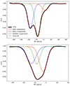 |
Fig. 1. Example of a triple-Gaussian fit to one of the CCF profiles for X Sgr (top panel) and BG Cru (bottom panel). |
In the second approach, we traced the hump formed between the two components of the line relatively to the mean RV of the CCF. The position of the hump is marked with a green vertical line in Fig. 2. We fit a single-Gaussian profile to each CCF (red dashed line in Fig. 2), which provided the RV determination. The RV of the hump was identified as the maximum of the residuals (blue dotted line above the CCF profile in Fig. 2). The relative RV of the hump was identified as the difference between the maximum of the residuals and the RV of the CCF profile from the Gaussian fit. We then constructed a time series representing the measured relative RV of the hump and analyzed it using standard time-series analysis technique. The top panel of Fig. 2 presents this approach for X Sgr, while the bottom panel presents it for BG Cru. We note that in the case of X Sgr we trace only the dominant hump that distorts the center of the CCF, even if there appears to be another hump at the wing.
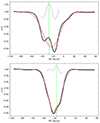 |
Fig. 2. Example of tracing a hump on the CCF profile for X Sgr (top panel) and BG Cru (bottom panel). |
In the third approach, we analyzed CCFs of X Sgr and BG Cru with FAMIAS (Zima 2008). We studied 2D frequency spectra, which allow us to see how the power is distributed along the CCF profile (see Fig. 13). We also performed consecutive pre-whitening using 1D average pixel-by-pixel spectra, which are calculated from the 2D spectra by averaging the amplitude across the profile for each frequency (see the top panel of Fig. 13). For this analysis, we only used CCF profiles collected with Coralie14. We note that it was not possible to reach the noise level in the pre-whitening procedure. After several pre-whitening steps, the highest detected signal in the frequency spectrum of the residuals was the residual signal at the position of the main radial mode. In Sect. 3, we report and discuss only the signals that were detected before this step.
2.2. Frequency analysis
We performed a frequency analysis of several different time series. We used the RV and CCF profile-shape indicators: FWHM, BIS (see Fig. 2 in Anderson et al. 2016), EW, and contrast as collected by VELOCE. We also constructed a few additional time series as described in Sec. 2.1 to specifically trace the periodicity of the hump in CCFs.
To find the dominant periodicity, we performed a standard Fourier analysis. In the case of RV, FWHM, BIS, EW and contrast, the dominant periodicity corresponded to the main pulsation mode. We subtracted the pulsation frequency and its harmonic from the data by fitting and subtracting a Fourier series in the following form:
where A0 is the mean value, fk is a dominant frequency of a radial mode and its harmonics, and Ak and ϕk are their amplitudes and phases. Then, we repeated the Fourier analysis of the residuals to search for any additional periodicities. We note that since VELOCE is a ground-based survey, there are also daily and yearly aliases in frequency spectra, which need to be taken into consideration when analyzing origin of the signals.
In the case of two additional time series constructed as described in Sect. 2.1, that is the RVs for each Gaussian component and the hump, we calculated frequency spectra to identify the dominant periodicity of the datasets. We note that in this case, the dominant signal no longer corresponds to the pulsation frequency.
2.3. Search for more stars showing the phenomenon
VELOCE collected observations for 258 classical Cepheids, and we searched for line-splitting patterns among all of them. We visually inspected all available CCFs collected by VELOCE for all of the monitored Cepheids and manually classified stars where the CCF profiles indicate presence of line splitting. We note, however, that this phenomenon is strongest in the cases of X Sgr and BG Cru. In the case of some stars in our sample, we noticed additional distortions and humps in the CCF profiles, suggesting unresolved, or marginally resolved, line-splitting patterns (see Figure 6 in Sect. 3 for LR TrA, V0411 Lac, V1334 Cyg, SZ Cas, ASAS J174603−3528.1, and V1019 Cas). CCF shape indicators for V0411 Lac were already analyzed by Netzel et al. (2024). In this work, we performed a frequency analysis of CCF parameters for the remaining candidates and we report our results for one of them (SZ Cas; see Sect. 3.2 for details). The data used for this star are also included in Tables 1 and 2.
3. Results
3.1. Occurrence of humps and splitting patterns
Line splitting in CCFs is the most prominent in the case of X Sgr among classical Cepheids studied in the literature and based on our sample of classical Cepheids observed by VELOCE. Interestingly, in the case of X Sgr, line splitting is not limited to one phase of pulsation. In fact, VELOCE data for X Sgr cover consecutive pulsation cycles thanks to the 7.01 d pulsation period, which allows us to investigate what the CCFs look like for similar phases of pulsation in consecutive cycles. This is presented in Fig 3 for phases ϕ ≈ 0.10, 0.38, 0.70, and 0.83 for at least two consecutive cycles. It is clear that CCFs from different cycles are significantly different from each other. The line splitting manifests differently even during the same pulsation phases. Hence, line splitting is neither limited to specific pulsation phases nor repeated on the timescale of the main pulsation mode as one would expect if it was connected to shock waves. In Fig. 4, we plot CCFs from two full consecutive cycles to further show the evolution of CCFs.
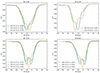 |
Fig. 3. CCFs of X Sgr around the same phases of pulsation for consecutive cycles. Different line colors correspond to different BJDs as indicated in the key. Phase of pulsation is marked above the panel. |
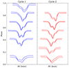 |
Fig. 4. CCFs from two consecutive cycles (one cycle per panel) plotted according to pulsation phase for X Sgr. |
In the case of BG Cru, we do not have data to plot the same phases of consecutive pulsation cycles. However, visual inspection of CCF profiles for similar phases of different cycles suggests, that this is also the case for BG Cru. Namely, the line splitting observed in BG Cru is also not limited to specific pulsation phases, but it is periodic, with a periodicity different than the main pulsation period. We plotted four consecutive cycles in Fig. 5: two cycles per panel. While consecutive cycles show some resemblance, there are already significant differences two cycles apart.
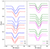 |
Fig. 5. CCFs from four consecutive cycles (C1, C2, C3, and C4) plotted according to pulsation phase for BG Cru (two cycles per panel). |
Signals found during the frequency analysis of RV data of X Sgr.
Anderson (2013) reported line splitting in LR TrA, which we can confirm using the currently available VELOCE data. Moreover, we found clear distortions of CCF profiles in five more Cepheids: V1334 Cyg, V0411 Lac, SZ Cas, V1019 Cas, and ASAS J174603−3528.1. In total, among 258 Cepheids from VELOCE, we found line splitting or unresolved line splitting in eight stars, which gives the incidence rate of approximately 3%. We plotted selected CCF profiles of LR TrA, V0411 Lac, V1334 Cyg, SZ Cas, V1019 Cas, and ASAS J174603−3528.1, which we show in Fig. 6, and we note that many of these stars are listed as modulators in Anderson et al. (2024). BG Cru and X Sgr are bright stars, with brightness levels in the V band of 5.47 mag and 4.58 mag, respectively. However, we detected similar features in stars as faint as 10 mag (for ASAS J174603−3528.1) or 11 mag (for V1019 Cas). Six out of eight stars with line splitting are first-overtone pulsators. Only two stars, X Sgr and SZ Cas, have dominant pulsations in the fundamental mode.
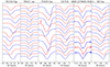 |
Fig. 6. Selected CCFs of stars with humps or line splitting: V1334 Cyg, V0411 Lac, V1019 Cas, LR TrA, ASAS J174603−3528.1, and SZ Cas. Colors and vertical shifts improve visualization. |
3.2. Frequency analysis of CCF shape indicators
In the first step of the frequency analysis, we used the RV provided by the VELOCE project, as well as the shape parameters FWHM, BIS, EW, and contrast, which were derived while measuring the RV for the VELOCE. The RV, FWHM, BIS, contrast, and EW time series of X Sgr phased with the dominant pulsation period and their corresponding frequency spectra after pre-whitening with the dominant frequency, f0, and its six harmonics are presented in Fig. 7. Clearly, an additional signal, fX, is present in frequency spectra of all datasets. In the case of RV data, two additional signals are present. In Table 3, we collect all signals detected in the frequency analysis of the RV data. Besides the two additional signals, fX and fY, we also detected a linear combination frequency, fX + f0, between fX and the dominant periodicity f0. The fX signal corresponds to the period of PX = 4.47 d and forms a period ratio of around 0.637 with the dominant pulsation mode.
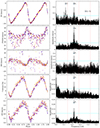 |
Fig. 7. Phased data and periodograms for X Sgr. Left panel: data for X Sgr phased with the dominant pulsation period. Consecutive rows present data for RV, FWHM, BIS, contrast, and EW. The BJD of each observation is color-coded. Right panel: frequency spectrum after pre-whitening with the dominant pulsation period and its harmonics. The position of the pulsation frequency and its harmonics are marked with red dotted lines. The additional signals are marked with arrows and labels (see also Table 3). The horizontal cyan line corresponds to three times the average noise level. |
X Sgr is plotted in the Petersen diagram (diagram of period ratio vs. longer period) in Fig. 8 with multimode groups of classical Cepheids. Interestingly, the period ratio formed by the fX with f0 fits the long-period extension of the so-called 0.61 Cepheids, in which the additional signal forms a period ratio of around 0.61–0.65 with the dominant first overtone (orange points in Fig. 8; for a review, see Netzel 2023 and references therein). The fY signal would fit relatively well as a subharmonic of the fX signal; that is fY/fX ≈ 0.528. However, the dominant pulsation mode of all currently known 0.61 Cepheids is the first overtone, while X Sgr primarily pulsates in fundamental mode (see RV curve characteristic for the fundamental mode in Fig. 7; Fourier coefficients of the RV curve (A1 = 12.55, R21 = 0.4029, ϕ21 = 3.1802, R31 = 0.1742, ϕ31 = 0.2980) are also consistent with values for the fundamental mode; see Figures 2 and 3 of Hocdé et al. 2024), which is an argument against classifying X Sgr as a 0.61 Cepheid. The most promising hypothesis explaining the origin of the signals in the 0.61 Cepheids is due to harmonics of nonradial modes of degrees 7, 8, or 9 (Dziembowski 2016). However, the period ratio between harmonics of these nonradial modes and the fundamental mode should be different from 0.61. Consequently, the additional signals detected in X Sgr likely have a different origin than in the case of the 0.61 Cepheids, if the hypothesis behind the 0.61 Cepheids is correct.
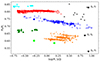 |
Fig. 8. Petersen diagram for multimode classical Cepheids. Different types of multi-periodicity are plotted with different colors and symbols. Blue circles: Pulsations in fundamental (F) mode and first overtone (1O). Red squares: Pulsations in 1O and second overtone (2O). Cyan asterisks: Pulsation in 2O and third overtone (3O). Green triangles: Pulsations in 1O and 3O. Lime diamonds: Pulsations in F and 2O. Orange points: 0.61 Cepheids. Grey pluses: Subharmonics in 0.61 Cepheids. Data are combined from different sources (see references in Netzel (2023)). Signals detected in X Sgr are plotted with black asterisks and are labeled. |
Phased RV, FWHM, BIS, and contrast for BG Cru is published in Fig. 1 of Netzel et al. (2024), where the additional signal forming a period ratio of around 0.61 was reported (see PX ≈ 2.03 d, i.e., 0.49 d−1, in Table 3 of Netzel et al. 2024). BG Cru pulsates in the first overtone and was also classified by Netzel et al. (2024) as a 0.61 Cepheid. The frequency analysis carried out by Netzel et al. (2024) revealed yet another additional signal with a frequency of fZ = 0.33235(3) d−1; that is close to the first-overtone frequency of f1O = 0.299 d−1. This signal is detectable in RV, FWHM, and BIS datasets. Interestingly, the fZ is the only additional signal detected in the BIS periodogram. Its origin, however, was uncertain and not analyzed by Netzel et al. (2024). In Sect. 3.2, we analyze whether the fZ signal can be connected to the observed line splitting. We note that, in addition to the analysis carried out in Netzel et al. (2024), we analyzed time series of EW. We did not detect any additional significant signals.
We also performed frequency analyses of RV, FWHM, BIS, and contrast data for the six stars where unresolved line splitting was detected. In the case of SZ Cas, we detected additional signal in the frequency analyses of FWHM and BIS. Frequency spectra after pre-whitening with the dominant fundamental mode and its harmonic are presented in Fig. 9. The SZ Cas fundamental-mode period is P0 = 13.638(1) d. The additional signal has a period of PX = 9.147(1). The shorter-to-longer period ratio is 0.67. The period and period ratio for SZ Cas do not correspond to any known groups of multimode classical Cepheids. Interestingly, this period ratio is relatively close to the position of subharmonic of the fundamental mode (i.e., 1.5f0). Still, it is unknown whether the additional periodicity is related to features observed in CCFs. Further observations are being collected to ascertain this. V0411 Lac was already analyzed by Netzel et al. (2024), which reported a detection of an additional signal that has a period longer than the first-overtone period, and both form a period ratio of around 0.687 (see discussion in Sect. 4.2). Besides X Sgr, BG Cru, SZ Cas, and V0411 Lac, we did not detect any additional signals in the rest of the stars with humps.
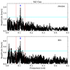 |
Fig. 9. Frequency spectra for SZ Cas after pre-whitening with fundamental mode and its harmonic, whose position is marked with red dotted lines. Additional signal is marked with the blue arrow. Top panel: frequency spectra calculated using FWHM time series. Bottom panel: frequency spectra calculated using BIS time series. |
3.3. Frequency analysis of the hump feature
The CCFs and spectral lines of X Sgr and BG Cru exhibit humps or more partially separated components. We traced the evolution of the principal hump feature as described in Sect. 2 and shown in Fig. 2. The frequency spectrum of the relative hump position is presented in Fig. 10 for BG Cru and X Sgr. The dominant signal in the frequency spectrum of X Sgr is fX Sgr = 0.08190(3) d−1, which corresponds to period of PX Sgr = 12.317(4) d. Interestingly, the signal detected in the frequency spectrum of RV, fX = 0.22382 d−1, is very close to the combination frequency between the signal detected in frequency spectrum of a hump and dominant fundamental-mode frequency (i.e., f0 + fX Sgr = 0.22450 d−1).
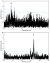 |
Fig. 10. Frequency spectra for time series of RV of hump in LPV (see text for details). The dominant signal is marked with the blue arrow. Top panel: frequency spectrum for X Sgr. Bottom panel: Frequency spectrum for BG Cru. |
In the case of BG Cru, the highest amplitude signal in the frequency spectrum of the hump time series is fBG Cru = 0.33243(10) d−1, which corresponds to the period of PBG Cru = 3.00813(9) d. Interestingly, the additional signal detected in frequency spectrum of RV, BIS, and FWHM has fZ = 0.33235(3) d−1 (PZ = 3.0088(3) d). Therefore, the periodicity detected in the frequency spectra of RV, BIS, and FWHM likely corresponds to the periodicity of the hump in CCF profiles.
3.4. Triple-Gaussian fit results
Last but not least, we analyzed the properties of the triple-Gaussian fits to CCFs. In the top panel of Fig. 11, we present centroids of the bluest, middle, and reddest Gaussian components from Fig. 1 phased with the dominant pulsation period of X Sgr (top panel) and BG Cru (bottom panel). The data phase well with the dominant period, as expected. However, there is a significant additional scatter visible for all datasets. This scatter is significantly stronger for the depth and width of the Gaussian components. Consequently, frequency analysis is hampered due to the relatively high noise level. The frequency analysis revealed the additional signals in some of the datasets, but only at a 3σ level. The detected signals in the case of X Sgr are fundamental mode frequency, fX Sgr (at the depths of the reddest and bluest components, in centroids of all components, and in the width of the bluest component; previously found in the analysis of the hump feature), fX (in the centroid of the middle component; found previously using line-shape indicators), f0 + fX (in centroid of the blue component; previously found using line-shape indicators), and f ≈ 0.047 d−1 (in the centroid of the blue component; not previously found). We note that some of these signals were detected only after pre-whitening with the dominant pulsation mode. Moreover, none of these signals exceed the 5σ detection level. In the case of BG Cru, we detected the first-overtone frequency and fBG Cru (in the depth and centroid of the red and middle components; previously found in the analysis of the hump feature). Again, none of the additional signals exceeded the 5σ level. In Fig. 12, we plot the strongest detection of an additional signal in all of the datasets created from the triple-Gaussian fit, which is for the depth of the bluest Gaussian component for X Sgr.
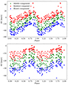 |
Fig. 11. Centroids of three Gaussians used for fit to CCF profiles phased with pulsation period for X Sgr (top panel) and BG Cru (bottom panel). Colors correspond to colors of the components in Fig. 1. |
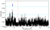 |
Fig. 12. Frequency spectrum of a depth of the bluest Gaussian component (see Fig. 1 and text for details) after pre-whitening with the fundamental mode. Arrows mark the fX Sgr signal. Red dotted lines marks the position of the fundamental mode frequency. Cyan lines correspond to three and five times the average noise level. |
3.5. Fourier spectra with FAMIAS
Two examples of 2D and 1D frequency spectra calculated for X Sgr with FAMIAS are presented in Fig. 13. Signals detected using previous methods are marked with arrows. In the left panels of Fig. 13, we plot frequency spectra of the original data. Clearly, the fundamental mode is visible. Also, the harmonic of the fundamental mode is visible in the 1D mean Fourier spectrum, which is less noisy compared to the 2D spectrum. However, based on the 2D spectrum, it is evident that the power is distributed asymmetrically across the CCF profile forming two asymmetric maxima. The same is barely visible for the harmonics of the fundamental mode. Interestingly, the first additional signal after pre-whitening with the fundamental mode and its harmonic is the signal at around 0.366 d−1, which corresponds to the combination frequency f0 + fX detected in the analysis of the RV data. Contrary to the radial mode, the highest amplitude is located at the center of the CCF. The list of frequencies detected using the 1D mean Fourier spectra is provided in Table 4. The fY signal found in the analysis of the RV data was not detected with the 1D mean Fourier spectra. We included two interpretations for the detected signal. In interpretation A, we assumed the independent signal fX = 0.22 d−1, as in the analysis of the RV data. Thus, the other signals are their combinations. In interpretation B, we adopted the highest additional signal as the independent periodicity (i.e., fX′=fX + f0). Unfortunately, it is not clear which scenario is correct and which signal is the independent periodicity. If the signals are due to nonradial modes, then it is possible for the combination frequencies to have higher amplitudes than the parent modes (see Benkő & Kovács 2023; Balona et al. 2013; Kurtz et al. 2015). Moreover, in the analysis of the hump position (see Sect. 3.3), we found a frequency of fX Sgr = 0.08 d−1, which was also detected in the 1D mean Fourier spectra as a combination frequency. Due to the fact that fX Sgr was detected by directly tracing the hump position in the CCF profile, it is a good candidate for an independent periodicity; however, this idea would need further confirmation.
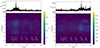 |
Fig. 13. Fourier spectra in 1D and 2D for X Sgr calculated based on Coralie14 CCFs using FAMIAS software. Left panels: frequency spectra of original data. Right panel: frequency spectra after pre-whitening with fundamental mode and its harmonic. Pre-whitened frequencies are marked in the bottom panel with red lines. Bottom panels: 2D spectra, where amplitude is color-coded. Frequencies found in other methods are marked with white arrows and labeled. Top panels: 1D mean Fourier spectra. |
Frequencies detected using pre-whitening of 1D mean Fourier spectra for Coralie14 CCFs of X Sgr.
4. Discussion
4.1. Line-shape indicators in case of split profiles
Line-shape indicators, in particular BISs, are well defined and easily calculated for CCFs and line profiles of the majority of classical Cepheids. However, in the case of strongly deformed profiles, as in the case of X Sgr, the definition of BIS is not as straightforward. We visualize this issue in the case of X Sgr in the top panel of Fig. 14. Namely, BIS is defined as midpoints of horizontal lines drawn across the CCF or line profile. In the case of a split profile, the bottom part of the profile consists of two dips, so the value of BIS is misrepresented as the line goes into one of the dips. To test whether using BIS for analysis in the case of X Sgr and BG Cru is substantiated, we visually inspected all calculated bisector lines for CCF profiles of X Sgr and flagged the cases when the profiles were split. Calculated BIS values phased with the fundamental period are plotted in the middle panel of Fig. 14, where the filled symbols correspond to the profiles where BIS could be easily calculated and open symbols are split profiles. The vast majority of points corresponding to the split profiles are outliers (many of them are not limited to the range shown in the phase plot) and do not phase well with the fundamental period. BIS values calculated from the regular profiles phase well with the fundamental period. Hence, the apparent noisiness of BIS in X Sgr is a consequence of line splitting, not of a poor signal-to-noise ratio (S/N) of the CCFs. We note that in the case of BG Cru there are fewer such outliers where the line splitting is less extreme. The frequency spectrum for X Sgr calculated using only the verified values of BIS is presented in the bottom panel of Fig. 14 and clearly shows the same additional signal as in Fig. 7. Removing the outliers connected to the split profiles lowered the overall noise level. However, even with the outliers caused by the split profiles, the BIS is proven to be a good dataset to search for additional signals.
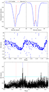 |
Fig. 14. Bisector inverse span (BIS) for X Sgr. Top panel: visualization of BIS in straightforward case (left) and in case of a split profile (right). Middle panel: phased BIS data for straightforward cases (filled symbols) and for split profiles (open symbols). Bottom panel: frequency spectrum after pre-whitening with the dominant frequency and its harmonics calculated using only the straightforward cases. |
4.2. The occurrence of line splitting in CCFs
We found line splitting or unresolved line splitting in eight stars out of 285 Cepheids monitored by VELOCE. Interestingly, the eight stars where line splitting or humps are unambiguously detected have relatively high values of average FWHM compared to the rest of classical Cepheids observed by VELOCE. This is presented in Fig. 15, where the average FWHM is plotted against the dominant pulsation period. The record holder is X Sgr, where the average FWHM is 40 km/s, while BG Cru and LR TrA have values of around 30 km/s. ASAS J174603−3528.1 is another star with a high average FWHM of 39 km/s. While its CCFs do not have the same quality as those of X Sgr, the humps in CCF profiles are clearly visible (see the fifth panel of Fig. 6). This preference for higher than average FWHM values suggests that line splitting might be correlated with high FWHM. It is not clear whether line splitting is connected to faster rotation manifesting as larger FHWM values, or if wider profiles make line splitting easier to detect. 24 Cepheids from our sample have literature values of v sin i, including X Sgr and BG Cru (Ammler-von Eiff & Reiners 2012). The literature values of v sin i cover a wide range from 3.3 km/s for MY Pup to 26 km/s for X Sgr, with a typical value of around 15 km/s for the sample. Interestingly, BG Cru also has one of the highest values of v sin i = 21 km/s.
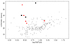 |
Fig. 15. Average FWHM calculated from all Gaussian fits to CCFs of classical Cepheids observed by VELOCE as a function of dominant pulsation period. Stars with regular CCF profiles are plotted with gray circles. X Sgr, BG Cru, and LR TrA are plotted with black squares. Additional selected candidates showing humps and line splitting in CCFs are plotted with red points. |
Additionally, these eight stars tend to have peak-to-peak amplitude of the RV curve from a lower half of the range defined by all 258 VELOCE Cepheids. Peak-to-peak amplitudes for all Cepheids and eight stars with line splitting or humps are plotted in Fig. 16. The highest values for the observed Cepheids are up to 61 km/s. None of the eight stars with (unresolved) line splitting have an amplitude higher than 29 km/s. The average depth for the sample is plotted in Fig. 17. Stars with (unresolved) line splitting have lower values than the rest of the sample. X Sgr has the lowest value among them – 10.6%. Moreover, none of the stars with humps or line splitting have an average depth higher than 20%.
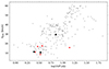 |
Fig. 16. Peak-to-peak amplitude of RV curve as function of dominant pulsation period for all classical Cepheids from VELOCE and stars with (unresolved) line splitting. Meanings of symbols are the same as in Fig. 15. |
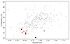 |
Fig. 17. Average contrast as function of dominant pulsation period for all classical Cepheids from VELOCE and stars with (unresolved) line splitting. Meanings of symbols are the same as in Fig. 15. |
Two stars are particularly interesting: V0411 Lac and SZ Cas. V0411 Lac was already analyzed by Netzel et al. (2024), who performed a frequency analysis of CCF shape indicators. The authors reported a detection of another low-amplitude additional signal that has a longer period than the first overtone and forms a period ratio of around 0.687 with the first overtone. This period ratio was already reported in the literature in some first-overtone classical Cepheids based on photometric observations, but the origin of the signal remains unknown (see a discussion in Netzel et al. 2024 and references therein). Here, we performed a frequency analysis for SZ Cas. The additional signal was detected in the FWHM and BIS data (see Sect. 3). The additional periodicity forms a period ratio of 0.67 with the main pulsation period. However, contrary to V0411 Lac, the additional signal has a period shorter than the main one. Unfortunately, the dataset currently available for V0411 Lac and SZ Cas is not numerous enough for analyses similar to those of X Sgr and BG Cru. Hence, we cannot confirm whether the periodicity detected by Netzel et al. (2024) in V0411 Lac and the signal detected in SZ Cas in this work are related to the observed humps in CCFs.
4.3. Interpretation of detected signals
In both X Sgr and BG Cru, we detected additional signals in frequency spectra of RV and CCF profiles shape indicators. Frequency analysis of photometric data for X Sgr collected by BRITE revealed additional signals as well (Smolec et al. 2018), which are equivalents of fY = 0.11815 d−1 and fX = 0.22382 d−1 detected in time series of RV, FWHM, BIS, EW, and contrast data of VELOCE. Possible hypotheses considered by Smolec et al. (2018) include pulsations in nonradial modes, periodic modulation, or contamination. The contamination scenario is unlikely, since we also independently detected these signals together with combination frequencies. We also did not find any star using the Gaia DR3 catalog (Gaia Collaboration 2023) within 2 arcsec of X Sgr, where this distance corresponds to the fiber size. We note, however, that X Sgr is bright, so the detection of any close companion would be significantly hampered. On the other hand, for a contaminating star to affect spectra, it would need to be considerably bright. In that case, such a star would also be expected to affect photometric light curves significantly, which is not the case. Consequently, the scenario of contamination is unlikely given the fact that the same signals are detected in both photometric and spectroscopic dataset. We did not notice any clear signature of long-term periodic modulation based on over ten years of VELOCE data either. From the interpretation of Smolec et al. (2018), we are left with nonradial modes. Moreover, Kovtyukh et al. (2003) also detected unexpected features in line profiles of X Sgr and BG Cru and proposed that their origins lie in pulsations in nonradial modes.
We note that in the case of BG Cru, there are multiple additional signals detected based on the frequency analysis of the CCF shape indicators (Netzel et al. 2024). One of them, fZ = 0.33235(3) d−1, corresponds exactly to the periodicity obtained through the analysis of the hump feature in the CCFs. Hence, we conclude that the detection of fZ in frequency spectra of RV, FWHM, and BIS is directly related to the line-splitting phenomenon visible in CCFs. However, fZ is not the highest amplitude additional signal in CCF shape indicators’ frequency spectra. Netzel et al. (2024) already reported an additional signal in BG Cru detected based on the frequency analysis of the FWHM and BIS data with a period of around 2.03 d. This forms a period ratio of around 0.61 and was already connected to likely pulsation in nonradial modes of moderate degrees of ℓ = 7, 8, 9 (Dziembowski 2016). Hence, fZ would be another nonradial mode present in BG Cru, if the interpretation of fZ is indeed due to nonradial mode. It is not clear however, which nonradial mode is at play.
On the other hand, Mathias et al. (2006) analyzed spectra of X Sgr and proposed that the observed line-splitting features in line profiles are due to pulsation-induced shock waves. In fact, the authors noticed that line profiles can be reproduced with not two but three components (see Fig. 1 of Mathias et al. 2006). Indeed, shock waves manifest in line profiles as line splitting, which is the case in other types of pulsating stars such as Miras or RR Lyrae stars (Alvarez et al. 2001; Fokin & Gillet 1994). However, pulsation-induced shock waves should be limited to specific phases of pulsation. This is not the case of X Sgr since its CCF profile’s appearance is significantly different for virtually the same pulsation phase (see Fig. 3). Moreover, we showed that changes in the hump feature (which appears when the profile is split) in X Sgr indeed has an underlying periodicity that is significantly different than the dominant pulsation period. Consequently, both observations effectively rule out the possibility that this phenomenon is caused by the pulsation-induced shock waves.
The periodicity of the hump in CCFs may in principle also arise as a result of a feature on the surface of a rotating star. Interestingly, tracing the relative position of the hump reveals a periodic phenomenon. Moreover, it appears that line splitting may correlate with the FWHM of the CCFs (see Sect. 4.2), indicating a possible link to rotation. Assuming the period–radius relations from Anderson et al. (2016), BG Cru and X Sgr would have radii of approximately 41 and 53 R⊙, respectively. For comparison, Li Causi et al. (2013) estimated R = 53 ± 3 R⊙ for X Sgr using long-baseline interferometric observations. Assuming a rotation period of 3 d for BG Cru would thus yield a very fast surface velocity of 110 km s−1, while for X Sgr, fX would correspond to veq = 96 km s−1 and f1 to veq = 35.8 km s−1. For comparison, the minimum FWHM of X Sgr’s CCFs is ∼34.1 km s−1, and it is 27.8 km s−1 for BG Cru, implying inclinations of i ≲ 15 − 20 degrees for both stars. Assuming a mass of ∼5, a spherical star of 50 R⊙ would have a first critical velocity ( ) of ∼140 km s−1. However, the predicted rotation rates of blue loop Cepheids formed from very fast rotating main-sequence stars are much lower than this, typically between 20 and 30 km s−1 (see Tables A.1 and A.4 in Anderson et al. 2016). Although an interpretation of fX in terms of surface rotation would yield a value lower than vc, it would nonetheless be a factor of 3 − 4 larger than predicted by single-star evolution models, thus making it necessary to invoke binary interactions. Neither X Sgr nor BG Cru are spectroscopic binaries (Anderson et al. 2024).
In Fig. 3, we show that CCFs of X Sgr look strikingly different for the same pulsation phases. In addition to this, in Fig. 18 we show what CCFs look like for the same phases when they are phased according to different additional signals that we found during our analysis. We considered fX and fY from the analysis of the shape indicators, the combination signal f0 + fX, and fX Sgr from the hump tracing analysis. For better visualization, all CCFs were shifted by the RV of each observation. It is clear that the CCFs (shifted to the mean velocity of each star) for similar phases are significantly different, regardless of the period used to calculate the phase. This shows that the changes in CCFs are either not strictly periodic or there are multiple periods at play.
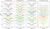 |
Fig. 18. CCFs of X Sgr phased based on four different periods indicated at the top of each panel. All CCFs are shifted according to RV for each observation. CCFs plotted here were collected for BJD from 2459338 to 2459383. Colors differentiate between different cycles. |
In Fig. 19, we plot CCFs of BG Cru, phased according to the period PBG Cru from the hump analysis, which was also independently found as PZ based on the CCF shape indicators. CCFs were also shifted according the RV for each observation. On the two different panels, we plot CCFs collected for five and 15 consecutive cycles of the additional periodicity. Clearly, the CCFs look similar for similar phases when we consider five cycles. On the other hand, when considering 15 consecutive cycles, some differences arise between the CCFs.
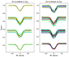 |
Fig. 19. CCFs of BG Cru phased based on period found in hump analysis. All CCFs are shifted according to RV for each observation. Colors differentiate between different cycles. Left panel: CCFs collected for BJD from 2459974 to 2459989 (five cycles of PZ). Right panel: CCFs collected for BJD from 2459974 to 2460019 (15 cycles of PZ). |
In BG Cru and X Sgr, the line-splitting phenomenon is very strong. Moreover, the data collected for BG Cru and X Sgr in VELOCE are numerous and have high signal-to-noise ratios since both stars are bright. Therefore, we were able to carry out a detailed analysis of the line-splitting phenomenon in both stars, resulting in the detection of the underlying periodicities. We note, however, that line splitting was also reported in several other stars in the literature. In particular, it was reported in LR TrA by Anderson (2013). Yet, the dataset available in VELOCE for LR TrA is not numerous enough –given that the line splitting is not as strong as in the case of X Sgr or BG Cru– to perform a similar frequency analysis. The VELOCE observations are ongoing, and we aim to repeat this analysis for LR TrA in the coming years.
Kovtyukh et al. (2003) also reported unexpected line-profile variations in EV Sct and V1334 Cyg. The latter star is also a part of the VELOCE database, and based on our dataset we also confirm the distortions of the CCF profiles (see Fig. 6). Unfortunately, the detailed analysis of the hump periodicity similar to that presented for X Sgr and BG Cru is not possible at present in the case of V1334 Cyg. More observations are being carried out in order to enable a similar detailed analysis.
4.4. Line splitting in spectral lines
CCFs benefit from very high signal-to-noise ratios, allowing for a detailed analysis of their shapes and variability. However, they come at a loss of information from individual lines. Interestingly, it was already reported that line splitting in metallic lines in X Sgr does not manifest in Balmer lines (Mathias et al. 2006). Using our spectra, we also confirm this for X Sgr.
Individual metallic lines are subject to relatively high noise. To compromise between investigating individual lines and benefiting from a high signal-to-noise ratio provided by the CCFs, we constructed two additional masks to calculate two additional sets of CCFs. The two additional masks were created based on the original G2 mask by selecting weak (depth < 0.55) and strong (depth > 0.65) lines. These masks were already used to investigate cycle-to-cycle modulations in long-period Cepheids by Anderson (2016). In Fig. 20, we plot CCFs based on the two masks for the same pulsation phases for X Sgr. We note that there is a difference in depth between weak and strong CCFs. CCFs based on weak lines are significantly more distorted than those calculated from strong lines. In particular, for phases ϕ = 0.84 and ϕ = 0.97 of the presented pulsation cycle, three components are clearly visible in the case of weak CCF, while only mild distortion is present in the case of strong the CCF.
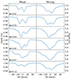 |
Fig. 20. Examples of CCFs for X Sgr calculated using the weak line mask (left) and strong line mask (right) for the same pulsation phases on one pulsation cycle. The pulsation phase is indicated in the bottom left corner of left panels. CCFs are shifted using the mean RV for better visualization of the shape variations. |
Weak metallic lines differ from the strong lines by their low and high excitation potentials. Consequently, weak metallic lines are more strongly constrained by the location in which they are formed. On the contrary, strong lines are formed over a larger range of optical depths. Hence, the line splitting is likely being averaged out over a larger part of an atmosphere than in the case of weak lines.
5. Conclusions
We analyzed line splitting present in BG Cru and X Sgr in detail using CCFs collected by the VELOCE project (Anderson et al. 2024). We also searched for more stars showing line splitting or humps in CCFs indicating the same phenomenon using all 258 classical Cepheids observed within the VELOCE project. Our findings and conclusions are as follows.
-
We show that CCFs differ significantly for the same pulsation phases of consecutive cycles for X Sgr. This rules out the possibility that the observed line splitting is connected to specific pulsation phases.
-
We traced the evolution of the hump formed by the line splitting by calculating its relative RV compared to the radial velocity of the Gaussian fit to the CCF. Frequency analysis of such time series revealed a periodicity of around 12 d for X Sgr.
-
The same analysis was performed for BG Cru and revealed the periodicity of the hump in CCFs of around 3 d. The same periodicity was detected in frequency spectra of CCF shape indicators (RV, FWHM, BIS) besides the dominant frequency of the radial mode, its harmonics, and the additional signal-forming-period ratio of around 0.61.
-
We performed a frequency analysis of CCF shape indicators for X Sgr, which revealed additional periodicities of 4.47 d and (only for RV) 8.46 d.
-
We detected similar CCF features in six more stars: LR TrA, SZ Cas, V0411 Lac, V1334 Cyg, V1019 Cas, and ASAS J174603−3528.1. In total, this gives eight stars with humps or line splitting selected from 258 classical Cepheids, which corresponds to the incidence rate of 3%. Among the eight stars, two are fundamental-mode stars (SZ Cas, X Sgr), and the remaining six are first-overtone pulsators.
-
Stars with humps or line splitting tend to have a higher average FWHM than is typical for classical Cepheids observed by the VELOCE project. The record holder is X Sgr, with 40 km/s, where the line-splitting phenomenon is the strongest.
-
Stars with humps or line splitting also tend to have peak-to-peak RV amplitudes below 30 km/s; that is, they have values from the lower half of the possible range defined by the VELOCE sample.
-
Stars with humps or line splitting also have a lower average contrast (below 20%) from the lower end of the distribution of the whole sample. The record holder is X Sgr, with just 10.6%.
-
Four stars out of eight show additional signals in frequency spectra of CCF shape indicators: BG Cru, X Sgr, V0411 Lac, and SZ Cas.
-
V0411 Lac has an additional long-period signal-forming-period ratio of 0.687 with the dominant first overtone. This star is a member of a group of multimode Cepheids showing this period ratio that were identified based on photometric observations.
-
SZ Cas show an additional shorter period low-amplitude signal that forms a period ratio of around 0.67. The origin of this periodicity is unknown.
-
We investigated how line splitting manifests as strong and weak metallic lines using modified masks to calculate CCFs for X Sgr. Line splitting manifests much more strongly in the case of weak metallic lines than in the case of strong ones. We confirm previous results that line splitting is not detected in Balmer lines.
VELOCE time series shed new light on the line splitting previously reported in individual Cepheids. We were able to study the phenomenon in great detail. Contrary to expectations, line splitting is unlikely to originate as a result of pulsation-induced shock waves: another mechanism must be at play. Particularly interesting is the connection between the additional signals found in periodograms with the line-splitting periodicity and the possible link between the line splitting and average FWHM. The ongoing VELOCE observations will allow us to investigate these intriguing discoveries further.
Data availability
The full Table 2 is available at the CDS via anonymous ftp to cdsarc.cds.unistra.fr (130.79.128.5) or via https://cdsarc.cds.unistra.fr/viz-bin/cat/J/A+A/694/A273
Acknowledgments
This work was supported by the European Research Council (ERC) under the European Union’s Horizon 2020 research and innovation programme (Grant Agreement No. 947660). RIA is funded by the SNSF through an Eccellenza Professorial Fellowship, grant number PCEFP2_194638. This work uses frequency analysis software written by R. Smolec. The Euler telescope is funded by the Swiss National Science Foundation (SNSF). Early VELOCE observations (2010 − 2016) were enabled by SNSF project funding from grant Nos. 119778, 130295, and 140893. This research is based on observations made with the Mercator Telescope, operated on the island of La Palma by the Flemish Community, at the Spanish Observatorio del Roque de los Muchachos of the Instituto de Astrofísica de Canarias. Hermes is supported by the Fund for Scientific Research of Flanders (FWO), Belgium, the Research Council of K.U. Leuven, Belgium, the Fonds National de la Recherche Scientifique (F.R.S.-FNRS), Belgium, the Royal Observatory of Belgium, the Observatoire de Geneève, Switzerland, and the Thüringer Landessternwarte, Tautenburg, Germany. We acknowledge the contributions of all observers who contributed to collecting the VELOCE dataset.
References
- Alvarez, R., Jorissen, A., Plez, B., et al. 2001, A&A, 379, 305 [NASA ADS] [CrossRef] [EDP Sciences] [Google Scholar]
- Ammler-von Eiff, M., & Reiners, A. 2012, A&A, 542, A116 [NASA ADS] [CrossRef] [EDP Sciences] [Google Scholar]
- Anderson, R. I. 2013, PhD Thesis, University of Geneva, Astronomical Observatory, Switzerland [Google Scholar]
- Anderson, R. I. 2016, MNRAS, 463, 1707 [NASA ADS] [CrossRef] [Google Scholar]
- Anderson, R. I. 2019, A&A, 623, A146 [NASA ADS] [CrossRef] [EDP Sciences] [Google Scholar]
- Anderson, R. I., Ekström, S., Georgy, C., et al. 2014, A&A, 564, A100 [NASA ADS] [CrossRef] [EDP Sciences] [Google Scholar]
- Anderson, R. I., Saio, H., Ekström, S., Georgy, C., & Meynet, G. 2016, A&A, 591, A8 [NASA ADS] [CrossRef] [EDP Sciences] [Google Scholar]
- Anderson, R. I., Viviani, G., Shetye, S. S., et al. 2024, A&A, 686, A177 [NASA ADS] [CrossRef] [EDP Sciences] [Google Scholar]
- Balona, L. A., Catanzaro, G., Crause, L., et al. 2013, MNRAS, 432, 2808 [CrossRef] [Google Scholar]
- Baranne, A., Queloz, D., Mayor, M., et al. 1996, A&AS, 119, 373 [NASA ADS] [CrossRef] [EDP Sciences] [Google Scholar]
- Benkő, J. M., & Kovács, G. B. 2023, A&A, 680, L6 [NASA ADS] [CrossRef] [EDP Sciences] [Google Scholar]
- Bono, G., Castellani, V., & Marconi, M. 2000, ApJ, 529, 293 [Google Scholar]
- Dziembowski, W. A. 2016, Commmunications of the Konkoly Observatory Hungary, 105, 23 [NASA ADS] [Google Scholar]
- Fokin, A. B., & Gillet, D. 1994, A&A, 290, 875 [NASA ADS] [Google Scholar]
- Fokin, A. B., & Gillet, D. 1997, A&A, 325, 1013 [NASA ADS] [Google Scholar]
- Gaia Collaboration (Vallenari, A., et al.) 2023, A&A, 674, A1 [NASA ADS] [CrossRef] [EDP Sciences] [Google Scholar]
- Hocdé, V., Moskalik, P., Gorynya, N. A., et al. 2024, A&A, 689, A224 [NASA ADS] [CrossRef] [EDP Sciences] [Google Scholar]
- Kovtyukh, V. V., Andrievsky, S. M., Luck, R. E., & Gorlova, N. I. 2003, A&A, 401, 661 [NASA ADS] [CrossRef] [EDP Sciences] [Google Scholar]
- Kraft, R. P. 1956, PASP, 68, 137 [NASA ADS] [CrossRef] [Google Scholar]
- Kurtz, D. W., Shibahashi, H., Murphy, S. J., Bedding, T. R., & Bowman, D. M. 2015, MNRAS, 450, 3015 [NASA ADS] [CrossRef] [Google Scholar]
- Leavitt, H. S. 1908, Annals of Harvard College Observatory, 60, 87 [Google Scholar]
- Leavitt, H. S., & Pickering, E. C. 1912, Harvard College Observatory Circular, 173, 1 [Google Scholar]
- Li Causi, G., Antoniucci, S., Bono, G., et al. 2013, A&A, 549, A64 [NASA ADS] [CrossRef] [EDP Sciences] [Google Scholar]
- Marconi, M., Musella, I., & Fiorentino, G. 2005, ApJ, 632, 590 [Google Scholar]
- Mathias, P., Gillet, D., Fokin, A. B., et al. 2006, A&A, 457, 575 [CrossRef] [EDP Sciences] [Google Scholar]
- Moskalik, P., Buchler, J. R., & Marom, A. 1992, ApJ, 385, 685 [NASA ADS] [CrossRef] [Google Scholar]
- Neilson, H. R., & Lester, J. B. 2008, ApJ, 684, 569 [NASA ADS] [CrossRef] [Google Scholar]
- Netzel, H. 2023, ArXiv e-prints [arXiv:2310.14824] [Google Scholar]
- Netzel, H., Anderson, R. I., & Viviani, G. 2024, A&A, 687, A118 [NASA ADS] [CrossRef] [EDP Sciences] [Google Scholar]
- Pepe, F., Mayor, M., Galland, F., et al. 2002, A&A, 388, 632 [NASA ADS] [CrossRef] [EDP Sciences] [Google Scholar]
- Queloz, D., Mayor, M., Udry, S., et al. 2001, The Messenger, 105, 1 [NASA ADS] [Google Scholar]
- Raskin, G., van Winckel, H., Hensberge, H., et al. 2011, A&A, 526, A69 [CrossRef] [EDP Sciences] [Google Scholar]
- Riess, A. G., Casertano, S., Yuan, W., et al. 2021, ApJ, 908, L6 [NASA ADS] [CrossRef] [Google Scholar]
- Sasselov, D. D., & Lester, J. B. 1990, ApJ, 362, 333 [NASA ADS] [CrossRef] [Google Scholar]
- Schwarzschild, M. 1952, in Transactions of the IAU, ed. P. T. Oosterhoff (Cambridge: Cambridge University Press), VIII, 811 [Google Scholar]
- Semenova, A. 2006, PhD Thesis, Germany [Google Scholar]
- Smolec, R. 2017, MNRAS, 468, 4299 [NASA ADS] [CrossRef] [Google Scholar]
- Smolec, R., Moskalik, P., Evans, N. R., Moffat, A. F. J., & Wade, G. A. 2018, in 3rd BRITE Science Conference, eds. G. A. Wade, D. Baade, J. A. Guzik, & R. Smolec, 8, 88 [Google Scholar]
- Soszyński, I., Udalski, A., Szymański, M. K., et al. 2015, Acta Astron., 65, 297 [NASA ADS] [Google Scholar]
- Süveges, M., & Anderson, R. I. 2018a, MNRAS, 478, 1425 [CrossRef] [Google Scholar]
- Süveges, M., & Anderson, R. I. 2018b, A&A, 610, A86 [NASA ADS] [CrossRef] [EDP Sciences] [Google Scholar]
- Zima, W. 2008, Communications in Asteroseismology, 157, 387 [NASA ADS] [Google Scholar]
All Tables
Frequencies detected using pre-whitening of 1D mean Fourier spectra for Coralie14 CCFs of X Sgr.
All Figures
|
Fig. 1. Example of a triple-Gaussian fit to one of the CCF profiles for X Sgr (top panel) and BG Cru (bottom panel). |
| In the text | |
|
Fig. 2. Example of tracing a hump on the CCF profile for X Sgr (top panel) and BG Cru (bottom panel). |
| In the text | |
|
Fig. 3. CCFs of X Sgr around the same phases of pulsation for consecutive cycles. Different line colors correspond to different BJDs as indicated in the key. Phase of pulsation is marked above the panel. |
| In the text | |
|
Fig. 4. CCFs from two consecutive cycles (one cycle per panel) plotted according to pulsation phase for X Sgr. |
| In the text | |
|
Fig. 5. CCFs from four consecutive cycles (C1, C2, C3, and C4) plotted according to pulsation phase for BG Cru (two cycles per panel). |
| In the text | |
|
Fig. 6. Selected CCFs of stars with humps or line splitting: V1334 Cyg, V0411 Lac, V1019 Cas, LR TrA, ASAS J174603−3528.1, and SZ Cas. Colors and vertical shifts improve visualization. |
| In the text | |
|
Fig. 7. Phased data and periodograms for X Sgr. Left panel: data for X Sgr phased with the dominant pulsation period. Consecutive rows present data for RV, FWHM, BIS, contrast, and EW. The BJD of each observation is color-coded. Right panel: frequency spectrum after pre-whitening with the dominant pulsation period and its harmonics. The position of the pulsation frequency and its harmonics are marked with red dotted lines. The additional signals are marked with arrows and labels (see also Table 3). The horizontal cyan line corresponds to three times the average noise level. |
| In the text | |
|
Fig. 8. Petersen diagram for multimode classical Cepheids. Different types of multi-periodicity are plotted with different colors and symbols. Blue circles: Pulsations in fundamental (F) mode and first overtone (1O). Red squares: Pulsations in 1O and second overtone (2O). Cyan asterisks: Pulsation in 2O and third overtone (3O). Green triangles: Pulsations in 1O and 3O. Lime diamonds: Pulsations in F and 2O. Orange points: 0.61 Cepheids. Grey pluses: Subharmonics in 0.61 Cepheids. Data are combined from different sources (see references in Netzel (2023)). Signals detected in X Sgr are plotted with black asterisks and are labeled. |
| In the text | |
|
Fig. 9. Frequency spectra for SZ Cas after pre-whitening with fundamental mode and its harmonic, whose position is marked with red dotted lines. Additional signal is marked with the blue arrow. Top panel: frequency spectra calculated using FWHM time series. Bottom panel: frequency spectra calculated using BIS time series. |
| In the text | |
|
Fig. 10. Frequency spectra for time series of RV of hump in LPV (see text for details). The dominant signal is marked with the blue arrow. Top panel: frequency spectrum for X Sgr. Bottom panel: Frequency spectrum for BG Cru. |
| In the text | |
|
Fig. 11. Centroids of three Gaussians used for fit to CCF profiles phased with pulsation period for X Sgr (top panel) and BG Cru (bottom panel). Colors correspond to colors of the components in Fig. 1. |
| In the text | |
|
Fig. 12. Frequency spectrum of a depth of the bluest Gaussian component (see Fig. 1 and text for details) after pre-whitening with the fundamental mode. Arrows mark the fX Sgr signal. Red dotted lines marks the position of the fundamental mode frequency. Cyan lines correspond to three and five times the average noise level. |
| In the text | |
|
Fig. 13. Fourier spectra in 1D and 2D for X Sgr calculated based on Coralie14 CCFs using FAMIAS software. Left panels: frequency spectra of original data. Right panel: frequency spectra after pre-whitening with fundamental mode and its harmonic. Pre-whitened frequencies are marked in the bottom panel with red lines. Bottom panels: 2D spectra, where amplitude is color-coded. Frequencies found in other methods are marked with white arrows and labeled. Top panels: 1D mean Fourier spectra. |
| In the text | |
|
Fig. 14. Bisector inverse span (BIS) for X Sgr. Top panel: visualization of BIS in straightforward case (left) and in case of a split profile (right). Middle panel: phased BIS data for straightforward cases (filled symbols) and for split profiles (open symbols). Bottom panel: frequency spectrum after pre-whitening with the dominant frequency and its harmonics calculated using only the straightforward cases. |
| In the text | |
|
Fig. 15. Average FWHM calculated from all Gaussian fits to CCFs of classical Cepheids observed by VELOCE as a function of dominant pulsation period. Stars with regular CCF profiles are plotted with gray circles. X Sgr, BG Cru, and LR TrA are plotted with black squares. Additional selected candidates showing humps and line splitting in CCFs are plotted with red points. |
| In the text | |
|
Fig. 16. Peak-to-peak amplitude of RV curve as function of dominant pulsation period for all classical Cepheids from VELOCE and stars with (unresolved) line splitting. Meanings of symbols are the same as in Fig. 15. |
| In the text | |
|
Fig. 17. Average contrast as function of dominant pulsation period for all classical Cepheids from VELOCE and stars with (unresolved) line splitting. Meanings of symbols are the same as in Fig. 15. |
| In the text | |
|
Fig. 18. CCFs of X Sgr phased based on four different periods indicated at the top of each panel. All CCFs are shifted according to RV for each observation. CCFs plotted here were collected for BJD from 2459338 to 2459383. Colors differentiate between different cycles. |
| In the text | |
|
Fig. 19. CCFs of BG Cru phased based on period found in hump analysis. All CCFs are shifted according to RV for each observation. Colors differentiate between different cycles. Left panel: CCFs collected for BJD from 2459974 to 2459989 (five cycles of PZ). Right panel: CCFs collected for BJD from 2459974 to 2460019 (15 cycles of PZ). |
| In the text | |
|
Fig. 20. Examples of CCFs for X Sgr calculated using the weak line mask (left) and strong line mask (right) for the same pulsation phases on one pulsation cycle. The pulsation phase is indicated in the bottom left corner of left panels. CCFs are shifted using the mean RV for better visualization of the shape variations. |
| In the text | |
Current usage metrics show cumulative count of Article Views (full-text article views including HTML views, PDF and ePub downloads, according to the available data) and Abstracts Views on Vision4Press platform.
Data correspond to usage on the plateform after 2015. The current usage metrics is available 48-96 hours after online publication and is updated daily on week days.
Initial download of the metrics may take a while.