| Issue |
A&A
Volume 690, October 2024
|
|
|---|---|---|
| Article Number | A284 | |
| Number of page(s) | 21 | |
| Section | Stellar structure and evolution | |
| DOI | https://doi.org/10.1051/0004-6361/202450185 | |
| Published online | 17 October 2024 | |
VELOcities of CEpheids (VELOCE)
II. Systematic search for spectroscopic binary cepheids
1
Institute of Physics, École Polytechnique Fédérale de Lausanne (EPFL), Observatoire de Sauverny, 1290 Versoix, Switzerland
2
Département d’Astronomie, Université de Genève, Chemin Pegasi 51, 1290 Versoix, Switzerland
3
Instituut voor Sterrenkunde, KU Leuven, Celestijnenlaan 200D bus 2401, Leuven 3001, Belgium
4
Smithsonian Astrophysical Observatory, MS 4, 60 Garden St., Cambridge, MA 02138, USA
5
Konkoly Observatory, HUN-REN Research Centre for Astronomy and Earth Sciences, MTA Centre of Excellence, Konkoly Thege Miklós út 15-17, H-1121 Budapest, Hungary
Received:
29
March
2024
Accepted:
29
May
2024
Abstract
Classical Cepheids provide valuable insights into the evolution of stellar multiplicity among intermediate-mass stars. Here, we present a systematic investigation of single-lined spectroscopic binaries (SB1s) based on high-precision velocities measured by the VELOcities of CEpheids (VELOCE) project. We detected 76 (29%) SB1 systems among the 258 Milky Way Cepheids in the first VELOCE data release, 32 (43%) of which were not previously known to be SB1 systems. We determined 30 precise and three tentative orbital solutions, 18 (53%) of which are reported for the first time. This large set of Cepheid orbits provides a detailed view of the eccentricity e and orbital period Porb distribution among evolved intermediate-mass stars, ranging from e ∈ [0.0, 0.8] and Porb ∈ [240, 9000] d. The orbital motion on timescales exceeding the 11 yr VELOCE baseline was investigated using a template-fitting technique applied to literature data. Particularly interesting objects include (a) R Cru, the Cepheid with the shortest orbital period in the Milky Way (∼238 d); (b) ASAS J103158−5814.7, a short-period overtone Cepheid exhibiting time-dependent pulsation amplitudes as well as orbital motion; and (c) 17 triple systems with outer visual companions, among other interesting objects. Most VELOCE Cepheids (21/23) that exhibit evidence of a companion based on a Gaia proper motion anomaly are also spectroscopic binaries, whereas the remaining do not exhibit significant (> 3σ) orbital radial velocity variations. Gaia quality flags, notably the renormalized unit weight error (RUWE), do not allow Cepheid binaries to be identified reliably although statistically the average RUWE of SB1 Cepheids is slightly higher than that of non-SB1 Cepheids. A comparison with Gaia photometric amplitudes in G-, Bp, and Rp also does not allow one to identify spectroscopic binaries among the full VELOCE sample, indicating that the photometric amplitudes in this wavelength range are not sufficiently informative of companion stars.
Key words: binaries: general / binaries: spectroscopic / stars: oscillations / stars: variables: Cepheids
Corresponding authors; This email address is being protected from spambots. You need JavaScript enabled to view it. ; This email address is being protected from spambots. You need JavaScript enabled to view it. ; This email address is being protected from spambots. You need JavaScript enabled to view it.
© The Authors 2024
 Open Access article, published by EDP Sciences, under the terms of the Creative Commons Attribution License (https://creativecommons.org/licenses/by/4.0), which permits unrestricted use, distribution, and reproduction in any medium, provided the original work is properly cited.
This article is published in open access under the Subscribe to Open model. This email address is being protected from spambots. You need JavaScript enabled to view it. to support open access publication.
1. Introduction
Classical Cepheids (henceforth: Cepheids) are evolved, luminous, intermediate-mass (∼3–11 M⊙), radially pulsating stars. For more than a century, Cepheids have been crucial calibrators of the extragalactic distance scale (Hertzsprung 1913) thanks to the famous period-luminosity relation (PLR or Leavitt law, Leavitt & Pickering 1912). The unceasing interest in Cepheids is not only due to their cosmological relevance, but also because these are crucial populations to understand stellar physics and they are important tracers in galactic studies (Luck & Lambert 2011; Genovali et al. 2014; Poggio et al. 2021; Kovtyukh et al. 2022, and references therein).
Given the importance of Cepheids as distance tracers, many astrophysical effects have been explored as potential biases of the Leavitt law, including multiplicity (e.g., Mochejska et al. 2000; Kiss & Bedding 2005). For certain individual Cepheids, light contributed by companions can indeed affect distance estimates; the most extreme cases of this include V1334 Cyg in the Milky Way (Gallenne et al. 2018) and a sample of Cepheids with double-lined spectroscopic companions in the Large Magellanic Cloud (which are indeed selected using their Leavitt law outlier nature Pilecki et al. 2021). However, Anderson & Riess (2018) showed that statistically speaking, Cepheid companions cannot bias the extragalactic distance scale or the Hubble constant measured therefrom. A similar result was recently obtained using population synthesis (Karczmarek et al. 2022). However, orbital motion on timescales of up to several years may affect the accuracy of parallax measurements of Cepheids (Anderson et al. 2015, 2016a; Benedict et al. 2022).
Parallaxes of Cepheids provided by the third data release (DR3) of the ESA mission Gaia do not yet account for orbital motion due to companions. However, this is expected to be available in future data releases, and DR3 already provided a large number of non-variable stars with non-single star solutions (Gaia Collaboration 2023). Combining astrometric and radial velocity data to determine orbits is particularly useful because it allows the total mass of a system to be measured (e.g., Gallenne et al. 2019) and thus provides key information for constraining stellar models in the context of the mass discrepancy problem (e.g., Caputo et al. 2005; Anderson et al. 2016b).
In the past few decades, numerous complementary techniques have been used for the detection of Cepheid binarity and multiplicity. Direct spectroscopic identification of low-mass companions at any separation is possible using X-ray and ultraviolet (UV) observations (Evans 1992; Evans et al. 2013, 2022). The detection of orbital motion through radial velocity (RV) variations is effective for a wide range of companion masses and spectral types; however, it necessitates long temporal baselines (Evans et al. 2015; Anderson et al. 2016a). Conversely, photometric binary detection methods, such as those using photometric amplitudes (Coulson & Caldwell 1985; Klagyivik & Szabados 2009) or photometric colors and ratios of amplitudes of different colors (Gieren 1985), require confirmation of the binary detection through subsequent spectroscopic investigations. Cepheid companions can also be detected using optical long-baseline interferometry, if the contrast and angular separation between the Cepheid and its companion are sufficiently small (Gallenne et al. 2014a, 2015, 2016, 2019).
Gaia proper motions have been introduced as indicators of multiplicity (Kervella et al. 2019a,b, 2022). While proper motion analysis is a powerful tool to detect resolved companions, it cannot be applied to the brightest stars that saturate the Gaia detectors. Furthermore, Gaia astrometric quality flags such as the reduced χ2 statistic are used as indicators of binarity assuming that the orbital motion leads to a photocenter wobble (Belokurov et al. 2020; Stassun & Torres 2021). In fact, several cuts on Gaia quality flags such as the RUWE and astrometric excess noise have been defined to filter the potentially multiple systems (Gaia Collaboration 2023). However, these cuts are established using stars where astrometric processing is simpler than in high-amplitude chromatically variable stars, such as classical Cepheids. It remains unclear if the same cuts can be applied to Cepheids, which are brighter than most stars used for calibrating Gaia systematics (cf. Khan et al. 2023 and references therein), and whose variability can cause excess noise in astrometric measurements.
The traditional approach of RV variations provides an unambiguous detection of a binary companion and helps the orbital parameters to be constrained. Dedicated RV monitoring campaigns have unraveled the orbital elements’ distribution of Cepheids (e.g., Evans et al. 2015; Szabados 2003). Low-mass companions such as the one of δ Cep (Anderson et al. 2015) or companions of fainter Cepheids (mV > 8 mag) require significant observational effort and precision to be detected, and this can only be achieved by long-term RV monitoring.
The VELOcities of CEpheids (VELOCE) project provides unprecedented RV time series of classical Cepheids (Anderson et al. 2024; Paper I henceforth). Taking advantage of the 11-year baseline of VELOCE, here we report the results of a systematic study of single-lined spectroscopic binaries (SB1s). Where the data allow it, we provide estimates of orbital periods, or describe the orbital motion using different methods. The paper is structured as follows. The observations and data analysis are presented in Section 2, in Section 3 we describe the different methods we used to analyze the SB1 Cepheids, followed by results in Section 4, which is divided into subsections for the results from each method used to describe the binary. In Section 5, we present the correlation between derived orbital parameters and compare our results with the Gaia binarity indicators. We briefly discuss and summarize this work in Section 6. The RV data as well as any fitted models, including orbital solutions and polynomial trends, used here are made publicly available as part of Paper I. In the appendix here (Appendix A) and in the on-line supplementary m aterial database1, we have presented supporting figures and tables. Lastly, in Appendix B, we provide detailed additional notes on individual systems.
2. Sample selection and available data
VELOCE comprises of precise Cepheid RV time-series data collected from both hemispheres using the high-resolution spectrographs Coralie (Queloz et al. 2001) and Hermes (Raskin et al. 2011). We used a minimum of 30 RV measurements per star, extending to up to 300 RV measurements for some cases. These observations cover a temporal baseline of nearly eleven years. Most of the VELOCE observations targeted signal-to-noise ratios (S/Ns) of at least 20, more commonly between 25 to 30, per pixel near 5500 Å. With such S/N we have typical RV uncertainties in the order of 50 ms−1. A detailed description of the observations and the RV data can be found in Paper I.
We identify SB1 candidates from 258 classical Cepheids observed by the VELOCE project (cf. Paper I for details) via time-variable pulsation-averaged velocities, vγ. Orbital motion in Cepheids introduces Doppler shifts on timescales of typically one year or longer that are mostly well separated from the pulsational timescales (of order days to months). Using VELOCE data, orbital motion can be detected in several different ways, depending on the availability and quality of the measurements (Section 3). The cleanest examples in our sample are Cepheids where clear, and possibly repeating, variations of vγ are discernible by eye in the pulsation (Fourier series) fit residuals. Such cases generally have orbital semi-amplitudes of several km s−1 and orbital periods of ≲3 yr.
While the selection function of Cepheids in VELOCE is rather complex, cf. Paper I, we consider VELOCE neither particularly biased toward the detection of SB1 systems, nor against it. For example, VELOCE initially specifically targeted Cepheids with no prior RV information and Cepheids residing near star clusters (Anderson et al. 2013). Later, Cepheids bright and nearby enough to measure interferometric radii were added (e.g. Anderson et al. 2016c; Breitfelder et al. 2016), and long-period Cepheids were targeted specifically for their use in distance ladder calibration (Anderson et al. 2016a). VELOCE also followed Cepheids with the goal of detecting modulated variability (e.g. Anderson 2014, 2016, 2019, 2020). Of course, stars found to exhibit orbital motion were followed up with the goal of characterizing orbits. However, only few stars were added to specifically search for suspected orbital signals.
Table 1 contains the list of stars considered in the present paper, ordered by whether their nature as spectroscopic binary was first reported here, was previously discussed in the literature. In Figure 1, we present the on-sky distribution of the sample SB1 Cepheids and the range in Gaia G mag that they span.
Sample of binary Cepheids and candidates from the literature considered here (excerpt).
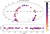 |
Fig. 1. Location of the sample SB1 Cepheids on the sky in the equatorial (top panel) and galactic (bottom panel) coordinate system. The symbols are color coded in the Gaia G magnitude. The symbols surrounded with blue circles are systems for which we provide an orbital solution in the current work. |
3. Data treatment and methods
3.1. RV curve models adopted
In most Cepheids, the RV variability due to pulsation dominates the RV time series with pulsational peak-to-peak amplitudes typically ranging from 20 − 70 km s−1. It is customary to model the pulsational variability using a Fourier series with a number of harmonics adapted to match the complexity of the RV variability. Paper I describes this process for all Cepheid RV curves in VELOCE. In short, the RV signal due to pulsation is modeled as:
 (1)
(1)
where n represents the order of the harmonic, t is time (in heliocentric Julian Date) and ϕ = (t − E)/Ppuls is the pulsation phase with epoch2E and the pulsation period, Ppuls. As described in Paper I, the optimal model is determined by fitting each RV time series using up to 20 Fourier harmonics and then performing model comparisons using the F-test and the Bayesian Information Criterion (BIC).
The key evidence of the spectroscopic binary nature presented here is a long-term modulation of vγ = vγ(t), typically on timescales > 1 yr and much longer than the pulsation period. We thus identify binaries by the correlated fit residuals they produce (Eq. 1). Orbital motion is then either modeled using a Keplerian orbit or approximated via linear, quadratic, or even higher order polynomials if the orbit is not sufficiently sampled to determine the full orbital solution.
As noted by Anderson (2014), Cepheids can exhibit modulated RV curves that can be misinterpreted as showing evidence of orbital motion. We note that all targets discussed here are bona fide spectroscopic binaries as identified by the absence of modulated line shape variability (Anderson 2016), although a few of the binaries presented here also show additionally modulated spectral variability. A detailed description of modulated RV variability of VELOCE Cepheids will be presented in future work.
3.2. Keplerian fitting
In the case of spectroscopic binaries, vγ = vγ(t) in Eq. (1) varies with time. The degree to which such variation can be used to infer the orbital elements depends largely on the sampling, baseline, and precision. Depending on these factors, we employed two methods for fitting Keplerian orbits to the data.
When fitting pulsational variability and orbital motion simultaneously, we fitted the Fourier series (Eq. (1)) and a Keplerian model simultaneously using the nonlinear least squares routine leastsq available in scipy.optimize (Virtanen et al. 2020). Following, for example, Hilditch (2001), the orbital motion is represented as:
![Mathematical equation: $$ \begin{aligned} v_\gamma (t) = v_{\gamma ,0} + K \left[\cos {\left(\omega + \theta \right)} + e \cos {\omega }\right], \end{aligned} $$](/articles/aa/full_html/2024/10/aa50185-24/aa50185-24-eq2.gif) (2)
(2)
where ω denotes argument of periastron, K semi-amplitude (in km s−1), e eccentricity, θ true anomaly, and vγ, 0 the systemic RV relative to the solar system barycenter. We note that vγ (without subscript 0) refers to the pulsation averaged velocity (cf. Paper I), which coincides with vγ, 0 if an orbital solution is determined or if the star does not have a companion. The uncertainties on the parameters are determined using the covariance matrix returned by the fitting routine, which incorporates statistical information on the reliability of the parameters estimated. Two examples of combined Fourier series plus Keplerian orbits for classical Cepheids are illustrated in Figures 2 and 3.
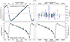 |
Fig. 2. Pulsation and orbital fit of the naked-eye Cepheid prototype δ Cephei. Left top: pulsation RV variability where the systemic velocity, vγ, 0 is indicated by a dashed line. Right top: residuals after fitting the Fourier series and Keplerian orbit against observation date. Left bottom: phase-folded orbital RV variation against orbital phase. Right bottom: orbital RV variation versus the observation date. |
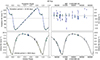 |
Fig. 3. Pulsation and orbital fit of one of the faintest binaries in our sample, NT Puppis. The figure description is the same as Figure 2. |
To understand and mitigate any dependence of our results on starting values, as well as to avoid convergence to a local minimum, we also implemented a Markov chain Monte Carlo (MCMC) method for determining Keplerian orbits. The MCMC fits further allow one to explore the posterior distribution of the orbital parameters to identify possible correlations and to rigorously quantify uncertainties (e.g. Ford 2005, 2006). However, we have not yet implemented an MCMC fit to simultaneously model pulsational and orbital variations; this is foreseen for future work. Thus, all MCMC orbital solutions presented here use template fitting residuals of VELOCE (cf. Section 5.1 of Paper I for more details) as well as literature radial velocity data, where pulsational variability has been removed (cf. Section 3.4). The MCMC orbits presented in this work utilize an extended baseline, achieved through the combination of VELOCE with literature datasets (V+L).
After testing different orbital parameterizations, we found that the following implementation converged the fastest (cf. also Fulton et al. 2018):
 (3)
(3)
where ϕ0 is the orbital phase to the next pericenter passage at t = E. We opted for a uniform prior for all parameters, and set sharp boundaries far away from possible solutions so that they would not alter the posterior distribution. Initial guesses were obtained by computing the Maximum A Posteriori (MAP)3 probability estimates from a grid of starting values of the parameters. The resulting orbits allowed us to visualize the possible different sets of parameters that could explain our data and have a sense of the stability of each solution by counting how many grid points converged to the same orbital parameters. We then chose the best parameters as the initial guess for our MCMC (an example of MCMC orbital fitting is provided in Figure 4).
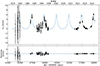 |
Fig. 4. Orbit of U Vul determined by fitting vγ epoch residuals of literature and VELOCE data. |
We used the MCMC implementation provided by the python package emcee (Foreman-Mackey et al. 2013) and, as suggested by the authors, used the autocorrelation time, τACT, to determine whether the chain was sufficiently long. In particular, the convergence criterion consisted of the following inequalities:
 (4)
(4)
 (5)
(5)
After running the MCMC, we visually inspected the resulting posterior distributions to check the absence of significantly non-Gaussian distributions (Figure 5). We also verified that the mean and standard deviation were compatible with the 16th, 50th, and 84th percentiles. We use the mean and standard deviation as the final results for the orbital estimates and its uncertainties. Finally, we also investigated circular orbits in a few cases where e was either very small or not significantly detected. In this case:
 (6)
(6)
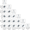 |
Fig. 5. Joint posterior distributions derived from the MCMC sampling for U Vul. The histograms show marginalized posterior distributions of the parameters. |
whereby ϕ0 represents the orbital phase to the next outgoing node at t = E.
Using orbital elements, we calculate the projected semimajor axis as:
![Mathematical equation: $$ \begin{aligned} a \sin {i}\,\mathrm{[au]} = \frac{1}{2\pi G} K\, P_{\rm orb}\, \sqrt{1-e^2}, \end{aligned} $$](/articles/aa/full_html/2024/10/aa50185-24/aa50185-24-eq7.gif) (7)
(7)
and the mass function as
![Mathematical equation: $$ \begin{aligned} f_{\mathrm{mass} }\,\mathrm{[M_\odot ]}= \frac{1}{2\pi G} K^3\, P_{\rm orb}\, {(1-e^2)}^\frac{3}{2}, \end{aligned} $$](/articles/aa/full_html/2024/10/aa50185-24/aa50185-24-eq8.gif) (8)
(8)
where G denotes the gravitational constant and the mass of the Sun was assumed to be M⊙ = 1.98840987 × 1030 kg (as used in astropy.constants).
3.3. Orbital trends represented using polynomials
Cepheids whose pulsation residuals computed using Eq. (1) indicated the presence of incompletely sampled orbital motion were modeled using the sum of Eq. (1) and a low-order polynomial of the form:
 (9)
(9)
The polynomial degree i adopted depends on the structure observed in the pulsation residuals (e.g., linear or nonlinear) and the overall vγ(t) variation over the VELOCE temporal baseline. We prioritized low values of i, typically < 3, and sought to obtain a reasonably close fit to the data. Additional data are required to determine full orbital solutions in these cases. It is important to note that in the present study, Fourier+polynomial fitting was exclusively employed for incompletely sampled orbits within VELOCE. This differs from the approach in Paper 1, where polynomials were utilized to represent modulated variability of any origin.
We note that vtrend(t) represents the change of the pulsation averaged velocity vγ(t) over time, so that vγ in Eq. (1) becomes the pulsation-averaged velocity near the midpoint of the RV time-series. Introducing such polynomials allows one to faithfully recover the pulsational variability and to partially quantify the orbital motion already sampled by the available data. However, it should be noted that in this case vγ is specific to the time-series and not generally valid for the star. Specifically, vγ then does not refer to the center of mass line-of-sight velocity of the system with respect to the Sun.
3.4. RV template fitting (RVTF)
We investigated variations of vγ over timescales exceeding the VELOCE baseline using RV datasets from the literature. To this end, we adopted the literature RV zero-point differences from Paper I and the RV template fitting (RVTF) approach developed in Anderson et al. (2016a), Anderson (2019). In this approach, the pulsational RV curve is assumed to be fully characterized by the high-quality pulsation fits obtained in Paper I using VELOCE data of each star. The template fitting technique then fits the VELOCE pulsation models to the available literature data while solving for two parameters, an offset in vγ(t) with respect to VELOCE, and a phase shift Δϕ. While the former is required to investigate binarity, the latter allows one to efficiently deal with pulsation periods changing over the course of several decades without having to assume a functional form for such period changes (cf. Section 5.2 of Paper 1).
In Paper I, we developed a semi-automated approach for clustering the available data sets using a Kernel Density Estimation algorithm whose bandwidth was varied according to data availability and quality. For binaries, we double checked the most appropriate bandwidth to use to avoid fitting data exhibiting significant variations of vγ as one epoch. Furthermore, we visually inspected all template fits to make sure they covered a sufficiently broad range in phase to be informative. Template fits restricted to an insufficiently narrow range in phase were discarded. For each clustered template fit and per literature reference, we obtained the mean date, range of dates, fit parameters Δvγ, Δϕ, their uncertainties, as well as the time-series epoch residuals (denoted as ϵvγ henceforth).
To investigate the significance of orbital signatures, we calculated the S/N between velocity offset and square-summed uncertainties as follows:
 (10)
(10)
where Δvγ is the difference between the zero-point-corrected4vγ obtained by template fitting and the pulsation averaged velocity from Paper I. σv denotes the uncertainty on vγ, and σvγ is the uncertainty on the instrumental zero-point correction vγ. Using Eq. (10), we searched for stars exhibiting deviations of more than S/NSB1 > 3 and rejected any spurious vγ variations among closely neighboring cluster sets following visual inspection, cf. Section 4.3.
Where feasible, we determined full orbital solutions using our MCMC algorithm (cf. Section 3.2) using the ϵvγ from template fitting as input. In practice, this often worked better than trying to fit a combined Fourier series and Keplerian model, since period changes could be effectively removed using the template fitting algorithm. The vγ and ϵvγ of literature datasets used in the orbital fits with MCMC algorithm and in the RVTF analysis are included in the VELOCE data files published as part of Paper I.
Please note that a thorough analysis comparing Gaia DR3 RVs with VELOCE RVs was performed in Paper I. The main arguments against including Gaia data in the current work were as follows: Firstly, their temporal baselines mostly overlapped with existing data, and no significant improvements in orbital coverage were identified. Secondly, we observed that certain stars displayed temporal trends in Gaia radial velocities (RVs) over timescales where VELOCE RVs showed no variations in pulsation-averaged velocity. However, a clear pattern regarding when and for which stars this occurred could not be discerned. In light of these disparities, Gaia RVs were omitted as a literature source for the spectroscopic binary search employing the method described above. With extended baselines, increased observation frequency, and improved data processing, future data releases with Gaia DR4 and DR5 are poised to excel in detecting SB1 systems and refining orbital solutions.
4. Results
This section describes the results of our systematic search for spectroscopic binary Cepheids using VELOCE data. An overview of the results is presented in Table 2. Tables 3 and 4 list orbital parameters for 18 Cepheids whose orbital parameters are being reported for the first time and 15 Cepheids whose orbits had previously been reported in the literature, respectively. The full versions of Tables 3 and 4 and figures illustrating the orbital solutions can be found with the supplementary m aterial available at the VELOCE zenodo repository5. Overall, we identified 76 bona fide SB1 Cepheids and 14 additional SB1 candidates in the VELOCE sample. 32 of these are reported as SB1 systems for the first time. Unless otherwise specified, we here discuss only bona fide SB1 Cepheids.
Overview of the results from the current work.
Orbital elements of the new spectroscopic binary Cepheids’ orbits presented in this work (excerpt).
Orbital elements of VELOCE SB1 Cepheids with literature-known orbits (excerpt).
We first discuss fully determined orbits in Section 4.1. Sections 4.2 and 4.3 present Cepheids with incompletely sampled orbits represented by polynomials and investigated using template fitting, respectively. We discuss the spectroscopic binary fraction in Section 4.4 and provide brief notes on individual Cepheids in Appendix B.
4.1. Full orbital solutions
This section presents the results obtained by fitting full orbital solutions to the RV time-series. We determined complete orbital solutions for 33 stars (including three tentative orbital fits). Section 4.1.1 begins with results based on VELOCE data alone, followed by results based on combined VELOCE and (zero-point offset-corrected) literature RVs in Section 4.1.2. Tables 3 and 4 distinguish these solution types using the tags “V” and “V+L”, respectively.
4.1.1. Orbits from VELOCE data alone (V)
Thanks to the high RV precision and data homogeneity, orbits derived using VELOCE data alone are typically very accurate. However, the available 11 yr baseline is not always sufficient to sample orbits fully, and occasional gaps in the time series may unfortunately coincide with particularly important orbital phases, preventing a definitive determination of all orbital parameters. All systems presented here were fitted using the combined Fourier series plus Keplerian model, which simultaneously solves for pulsational and orbital variability. The resulting orbital periods range from 237 to approximately 4000 days, that is, the baseline available from VELOCE DR1.
Figures 2 and 3 illustrate two examples of combined Fourier series plus Keplerian orbits for the naked-eye prototype of classical Cepheids, δ Cephei, and the faint southern target NT Puppis, cf. Appendix B for additional details. All the other combined fits can be found online6.
The choice of starting values for model fit parameters, notably Porb and e, can impact the determination of orbital solution. We therefore adopted reasonable starting values estimated by inspecting the Fourier series fit residuals. Where starting values could influence the result, we cross-checked the results using the MCMC template fitting algorithm, cf. Section 3.2. For most stars, however, the data set sampled the orbital cycles sufficiently well to allow an initial guess close to the correct orbital period.
The best fit orbital parameters obtained here generally agree with previous orbital solutions published in the literature despite improved uncertainties. However, we obtain significantly different orbital periods for six Cepheids δ Cep (cf. Figure 2), AX Cir, MU Cep, V1334 Cyg, W Sgr, and XX Cen. These stars, among others, are discussed in detail in Appendix B.
4.1.2. Orbits from VELOCE and literature data (V+L)
We determined orbital solutions using combined VELOCE and literature data using our MCMC algorithm applied to the template fitting epoch residuals; such fits are labeled as V+L in Tables 3 and 4. Orbits of five newly discovered binaries (FO Car, MY Pup, R Cru, VY Per, and VZ Pup) and nine previously known binaries (DL Cas, FF Aql, S Mus, S Sge, SY Nor, TX Mon, U Vul, V1334 Cyg, and YZ Car) were obtained using VELOCE data alone as well as in combination with literature RVs. The V and V+L orbits for 12 of these 14 agree within the uncertainties, although V+L orbits tend to have lower uncertainties, mostly due to better orbital sampling. The exceptions are MY Pup and VZ Pup. The VELOCE baseline only marginally covers the orbital period of MY Pup, hence, incorporating literature data results in a modification of the period. The Porb of VZ Pup differs by 2.4σ between V and V+L orbits due to the Porb being on the order of the available VELOCE baseline. The V+L result is thus clearly preferred, hence, whenever available we use V+L orbital estimates in any sample descriptions presented here. Lastly, for two stars, AX Cir and SU Cyg, we could only obtain a combined fit using VELOCE and literature data. In the case of AX Cir, due to its very long orbital period and for SU Cyg due to the incomplete sampling of orbital phase with VELOCE data alone.
4.1.3. “Tentative” orbits using VELOCE and literature data
We determined first tentative orbital solutions for three stars: BP Cir, R Mus, and V0659 Cen. We consider these orbits tentative because the literature data were not sufficiently constraining, while the VELOCE data alone were not sufficient to sample a full orbit. Additional observations are required to ascertain the true orbital solutions for these stars. Please note that the uncertainties associated with the orbital parameters of the tentative orbits listed in Table 3 may not accurately reflect the limitations arising from the insufficient sampling of these long orbits. The stated uncertainties are formal uncertainties on the model given the data. However, in cases of poor or incomplete orbital sampling, it is possible that the true orbital period is outside the range of these formal errors. This is why we present these cases separately as tentative.
4.2. Incompletely sampled orbits modeled as polynomial trends
We represented 16 newly detected SB1 systems and 14 previously reported SB1 systems using a combined Fourier series plus polynomial trend. Table 5 quantifies the measured range of the orbital RV variation, Ap2p, over the temporal baseline (denoted by ΔTp2p), which is the baseline of the observations over which the Ap2p was calculated. Among the 30 systems examined with Fourier plus polynomial fit, 15 Cepheids exhibit nonlinear trends. Among the 15 stars with linear trends, 5 demonstrate a decreasing trend in vγ, whereas the remaining 10 feature increasing vγ. Additional observations are required to determine these orbits.
List of SB1 from our sample where we found some evidence of orbital motion, and a polynomial was fitted as the orbit could not be sampled or covered adequately (excerpt).
Figure 6 presents the distribution of Ap2p versus ΔTp2p and the pulsation period. A clear trend of increasing Ap2p as we extend to longer temporal baselines is visible. For a fixed value of K, this trend arises because longer baselines increasingly sample the full (albeit incomplete) peak-to-peak variation of the orbit. However, there is significant dispersion in the value of K at fixed Porb due to different inclinations and mass ratio. The smallest trends of between 0.2–0.35 km s−1 are found for V1162 Aql, DR Vel, FR Car and SX Vel (over ∼1.8, 4.5, 5.8 and 5.9 yr respectively). By comparison, the smallest K among completely solved orbits is 0.67 km s−1 (MY Pup, 5.7 yr). At the long timescale limit, we find Ap2p = 1.2 km s−1 variation for T Mon over the course of nearly 10.5 yr. By comparison, the lowest K = 2.1 km s−1 for a completed orbit and a similar Porb of 11 yr is found for VZ Pup.
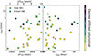 |
Fig. 6. Distribution of Ap2p, maximum amplitude variation in vγ, for the stars in our sample where we could fit a polynomial to the vγ trend (see Section 3.3 for details). In the left panel, we have the Ap2p vs the baseline in time over which it was calculated and in the right panel, the same against the pulsation period. The newly discovered SB1s from our sample are plotted in filled squares, while the literature-known SB1s are plotted in filled circles. The color bar represents the degree of polynomial fitted in the Fourier+Polynomial model. |
4.3. Template fitting for stars without orbital signatures in VELOCE data
Paper I presented a list of SB1 Cepheids exhibiting time-variable average velocities detected using VELOCE data alone. SB1 Cepheids with very long Porb could, however, remain undetected based on VELOCE data alone. Hence, we investigated the temporal stability of vγ for all Cepheids in VELOCE using the well-defined RV templates from Section 3.4. To this end, we computed S/NSB1 (Eq. 10) and considered a star a likely binary if any template fit resulted in a 3-σ deviation (S/NSB1 > 3) from a constant value of vγ.
Applying this method to 174 bona fide VELOCE Cepheids with available literature data resulted in the discovery of four additional SB1 candidates: β Dor, SZ Aql, V0402 Cyg, and X Cyg, cf. Figure 7. All four exhibit visually convincing trends in vγ on the order of 1 − 3 km s−1 on timescales exceeding 15 000 − 20 000 d.
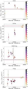 |
Fig. 7. Zero-point corrected Δvγ for new SB1s detected through RVTF. The dotted lines mark the standard deviation of the vγVELOCE. This figure only includes stars where we have a 3-σ detection through our analysis. The color bar represents the S/NSB1 of the various vγ measurements where the S/NSB1 was calculated as described in the text. |
Additionally, we found 8 bona fide SB1 Cepheids (CD Cyg, η Aql, RS Ori, SS CMa, SZ Cyg, V0340 Ara, V0916 Aql and VY Sgr) among a sample of 32 SB1 candidates previously reported in the literature (Szabados 2003) where the available baseline of VELOCE data alone was insufficient to detect orbital motion. Figure 8 illustrates these cases. CD Cyg and SS CMa were already discussed as potential SB1s from the RVTF analysis of Anderson et al. (2016a) using VELOCE data. Here, we confirm that the deviations in vγ indicate of binarity.
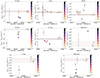 |
Fig. 8. Literature-known SB1 candidates detected through RVTF. The figure description is the same as Figure 7. |
For the remaining 24 Cepheids among the 32 candidates, we could not confirm unambiguous orbital motion despite large overlaps in the data used. Ten of these 24 Cepheids do not exhibit a S/NSB1 > 3, over a temporal baseline of 10 000–20 000 days. For the remaining 14 cases, individual vγ variations are found, although they should be considered spurious variations because closely neighboring vγ estimates clearly show the absence of a trend at these epochs. In the supplementary m aterial, we present all these non-SB1 cases and we have tagged these stars with RVTF-No in the Binarity column of Table 1.
Given the high accuracy of the VELOCE template fitting procedure, which effectively removes any pulsational variability and period variations, and since instrumental zero-point differences have been corrected using nonbinary Cepheids (cf. Paper I), we conclude that these 24 Cepheids should not be considered spectroscopic binaries.
4.4. SB1 fraction among VELOCE Cepheids
The 76 bona-fide SB1 Cepheids detected as part of VELOCE yield a lower limit to the spectroscopic binary fraction of 29.6 ± 3.4% that is fully consistent with the result by Evans et al. (2015) of 29 ± 8% based on the 40 brightest Cepheids. If all 14 SB1 candidates from Paper I should be confirmed to be bona-fide SB1 systems, then the VELOCE binary fraction would increase to ∼35%.
Using the subset of Cepheids with fully determined orbital solutions from Tables 3 and 4 and assuming that all undetermined orbits have very long orbital periods, we find a lower limit to the fraction of SB1 Cepheids with orbital periods of less than 10 yr of 15.2 ± 2.4%, slightly lower albeit consistent with the reported 20 ± 6% from Evans et al. (2015). Although our stringent template-based investigation (Section 4.3) questioned the veracity of the SB1 nature of 24 Cepheids for which such evidence had been previously discussed (cf. references in Szabados 2003), the fraction of SB1 systems among Cepheids we determined remains similar because we also identified new SB1 systems. However, the more accurate determination of time-variable vγ alongside detailed zero-point corrections affords much greater confidence in the determination of the SB1 nature of individual Cepheids. Of course, the SB1 fraction of Cepheids is merely a lower limit of the total fraction of Cepheids with companions due to the possibility of very large separations, unfavorable inclinations, and extreme mass ratios.
Figure 9 illustrates the magnitude distribution of newly discovered and detected SB1 Cepheids alongside the distribution of binary systems reported in the online compilation by Szabados (2003), as well as the distribution of magnitudes for which orbits were determined here. To ensure consistency in the comparison, we have exclusively included the bona-fide SB1 binaries from Szabados (2003) in Figure 9. Therefore, other types of binaries (such as photometric, visual, etc.) from their catalog are not accounted for in this analysis. Please note that Figure 9 does not include 24 systems that are not detected as SB1 in our study.
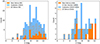 |
Fig. 9. Stacked histogram presenting the new VELOCE SB1 detections (left panel) and the new VELOCE orbits (right panel) along with the same thing from Szabados (2003). SY Nor’s orbit is provided by us as well as Bersier (2002); however, it is missing in the Szabados (2003) database. |
As the right panel of Figure 9 shows, we here double the number of orbital solutions for Cepheids fainter than ∼8-th magnitude, and there are only 14 Cepheids with known orbital solutions that are not included in this work (one Cepheid among these 14, namely T Mon has incompletely sampled orbit in this study). Conversely, we determine the first orbital solutions for 18 Cepheids, most of which fainter than ≳8 th magnitude.
5. Sample analysis
5.1. Correlations among orbital elements
Figure 10 shows the correlation between different orbital elements (ω, K, e, and a sin i) with Porb for all orbital solutions reported here. This includes first-time orbital estimates of 18 stars and 15 VELOCE orbital estimates for Cepheids with literature-known orbits. Newly discovered SB1 systems populate the full range of orbital parameters, indicating that our sample selection was not biased towards the literature-known orbital properties of SB1 Cepheids. Semi-amplitudes tend to decrease as Porb increases. Thanks to the precision of VELOCE RV measurements and long-term monitoring, we were able to discover many new SB1 systems with very small semi-amplitudes and long orbital periods. A noticeable correlation exists between a sin i and Porb, and the dispersion along this correlation might stem, at least partially, from fluctuations in the combined masses of the Cepheid and its companion.
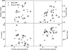 |
Fig. 10. Distribution of different orbital elements (Upper left: argument of periastron ω; upper right: eccentricity e; lower left: semi-amplitude K of the orbital RV variations; and lower right: projected semi-major axis a sin i) versus orbital period Porb for Cepheids with the orbits determined here. SB1s with newly reported orbits in this study are plotted using open squares, while VELOCE orbital estimates of SB1s with literature-known orbits are plotted in open circles. Symbols with double boundaries highlight V+L orbits determined using VELOCE and zero-point corrected literature RVs. R Cru, SY Nor and YZ Car are absent in the top left panel due to insignificant eccentricity. |
The eccentricity versus orbital period distribution (upper right panel in Figure 10) is particularly interesting. We find that the maximum eccentricity increases with orbital period. Despite a large range of eccentricities at most Porb values, an absence of very high e < 0.6 is clearly noticeable at Porb ≲ 3 yr. The two Cepheids with the shortest Porb have very low or no noticeable eccentricity. We also notice an absence of circular orbits at Porb ≳ 3 yr, which appears to become an exclusion region at longer Porb. Since such distant companions have most likely evolved in isolation, this could point to a primordial feature of intermediate-mass (B-star) binaries. However, NBODY simulations show that cluster dynamics increase e for long orbital periods over time (Dinnbier et al., in prep.). Additional long-period orbits are required to investigate this effect.
Most of these trends qualitatively agree with the empirical results by Evans et al. (2015), as well as with predictions from the Cepheid binary population synthesis study by Neilson et al. (2015) and Karczmarek et al. (2022), as well as with the dynamical NBODY6 simulations by Dinnbier et al. (2024). However, we do find several Cepheids at high 5 < Porb < 10 yr and relatively low eccentricities (e < 0.2) where Cepheid binaries have been predicted to have a low probability of occurring (Neilson et al. 2015). Additionally, R Cru is very close to the minimum Porb consistent with the synthetic populations by Neilson et al. (2015) and Karczmarek et al. (2022).
Incompletely sampled orbits described in Section 4.2 and illustrated in Figure 6 provide partial information on K and Porb. Comparing Ap2p with K (in Figure 10) as a function of Porb, we notice the inverse trends. Shorter orbital periods tend to have larger K, whereas we find larger Ap2p over longer baselines. This suggests that most short-Porb orbits with K ≳ 0.5 km s−1 of Cepheids observed by VELOCE have been determined. Very low Ap2p values are likely to continue growing over longer baselines.
5.2. Cepheids exhibiting proper motion anomaly
Kervella et al. (2022) used Gaia to detect astrometric binaries using the proper motion anomaly (PMa). This method compares the proper motion vector determined by the ESA HIPPARCOS mission (Perryman et al. 1997) and various Gaia data releases (Gaia Collaboration 2016a,b, 2018, 2021; Michalik et al. 2015; Lindegren et al. 2018, 2021). PMa quantifies the significance of a long-term rotation of the proper motion vector due to orbital motion. Stars with PMa signals exceeding 3σ were thus labeled as binaries by Kervella et al. (2022). Proper motion probes the on-sky projection of orbital motion, orthogonal to the line-of-sight variations measured using RVs. Therefore, the PMa and RV methods function as complementary tools for binary detection (cf. Kervella et al. 2019b for details on the sensitivity function of PMa). Consequently, it’s typical for some stars identified as SB1 to lack discernible deviations in their proper motions which would categorize them as PMa-True candidates. This could either be if the Cepheids are located at large distances or possess orbital periods too short for detection. On one hand, companions with orbital periods shorter than ∼3 years are unlikely to be identified via PMa due to the time window smearing inherent in Gaia DR3. On the other hand, extremely long-period companions, spanning hundreds of years, are similarly challenging to detect, representing a limitation shared by VELOCE as well. Importantly, a PMa-False flag does not raise concerns about the SB1 detection. Among the 76 binary Cepheids in our sample, 19 have been reported to exhibit PMa signals (with binary flag “BinH2EG3b” in Kervella et al. 2022 as 1)7. Evidence of astrometric orbital signals in form of the PMa has been reported for 10 of 33 SB1 (30%) Cepheids with orbital solutions presented here (including tentative ones) as well as for 8 of 30 (25%) SB1 systems with long-term vγ trends exhibit PMa (Kervella et al. 2022). This also includes 2 of the newly discovered SB1 Cepheids, GX Car and V0659 Cen.
Two systems with reported PMa, RZ Vel and SV Per, deserve a specific mention. For these two stars, we found no evidence of time-variable vγ. However, SV Per is known to have a very nearby (0.2″) companion that has been resolved using HST/WFC3 spatial scans (Riess et al. 2018) and which is most likely unresolved by Gaia. Time-variable contrast differences due to the Cepheid’s pulsation would affect the measurement of the photocenter for SV Per, which may lead to a spurious PMa signal.
Finally, we note that none of the Cepheids considered to be non-SB1s in VELOCE–stars without evidence of time-variable vγ-have been reported to exhibit a significant PMa. Specifically, this is true for all stars without evidence of time-variable vγ based on VELOCE data alone as well as our RVTF analysis (Sect. 3.4), including stars for which our results contradict previous claims of time-variable vγ.
As this comparison shows, RVs from VELOCE and literature data standardized to the VELOCE zero-points provide the most complete evidence of orbital motion for Cepheids on timescales of up to a few decades. Nonetheless, we caution that signals on the order of 1 km s−1 and lower can be introduced also by modulated variability (Anderson 2014). CCF shape parameters, such as the bisector inverse span and full width at half maximum can be informative to this end (Anderson 2016) and will be considered in future work.
5.3. Gaia DR3 astrometric quality flags of SB1 Cepheids
Gaia DR3 reports several astrometric quality flags and parameters to aid the interpretation of the reported astrometric measurements. The Renormalized Unit Weight Error (RUWE) has received particular attention and is often considered an indicator of stellar multiplicity. RUWE is calculated as the square root of the normalized χ-square of the astrometric fit to the along-scan observations (Lindegren 2018), and the threshold of RUWE < 1.4 is frequently used to indicate well-behaved astrometric solutions (Lindegren et al. 2018, 2021). However, several factors can result in elevated RUWE, which does not identify the origin of the excess residuals and includes all possible sources of error in the fit to the astrometric model. The latter include any signals affecting photocenter stability, notably involving marginally resolved visual binaries and unmodeled astrometric orbital signals.
In Cepheids, the high-amplitude chromatic variability of Cepheids could also contribute to RUWE. For example, Gaia may automatically select different gating schemes and window classes depending on the momentaneous brightness of Cepheids that vary by ∼1 mag in optical bands. Additionally, chromatic variability may lead to noise due to time-variable chromatic diffraction properties. Given these added difficulties, it is likely for RUWE to be elevated for Cepheids compared to non-variable stars. We therefore investigated to what degree excess RUWE and other astrometric quality indicators reported by Gaia may serve as an indicator of multiplicity for Cepheids.
Figure 11 shows the comparison of Gaia DR3 RUWE against the projected semimajor axis and Porb. The figure shows a significant excess RUWE near a sin i values close to 1 au as 5 out of 8 stars with the highest RUWE (RUWE > 2) fall into this category (stars located within the dashed red lines in the left panel of Figure 11). Interestingly, a corresponding feature is not so clearly seen near Porb = 1 yr, suggesting that the size of the orbital ellipse on the sky more directly affects the astrometric solution than the periodicity of the signal. The 6300 d binary with the highest RUWE of 7.8 is AX Cir, whose hot main sequence (likely B6V) companion has been resolved interferometrically (Gallenne et al. 2014b). A photometric contamination is the potential origin of the elevated Gaia RUWE.
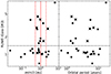 |
Fig. 11. Distribution of Gaia DR3 RUWE with the semi-major axis (left) and orbital period (right) of our sample systems. The stars tagged as binaries from PMa (Kervella et al. 2022) are marked with crosses. The red solid line indicates a sin i of 1 au, and the dashed red lines indicates the same at 0.5 and 2 au. |
Figure 12 shows RUWE in Gaia DR3 vs the amplitude of trends, Ap2p, determined using VELOCE data only in Sect. 4.2. Given that the majority of these orbital signals occur on timescales longer than the VELOCE baseline, it is not surprising that RUWE < 1.4 for the vast majority of these stars. The most significant outlier at RUWE ∼ 8 is RW Cam, which was shown to feature a significant UV excess indicative of a hot main sequence companion (Stepien 1968). The star with the second highest RUWE of 1.7 is T Mon, host to a B9.8V companion detected directly from UV spectroscopy (Evans & Lyons 1994) but remained undetected interferometrically in H-band (Gallenne et al. 2019). These stars collectively indicate that elevated Gaia RUWE values in Cepheids may be attributed to unresolved companions rather than orbital motion.
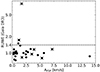 |
Fig. 12. Distribution of Gaia DR3 RUWE with the maximum amplitude of the (linear or nonlinear) vγ variation for SB1 systems with Trend. The stars tagged as binaries from PMa (Kervella et al. 2022) are marked with crosses. |
Figure 13 shows the probability density function of RUWE for SB1 and non-SB1 Cepheids in VELOCE. Approximately 25% of VELOCE SB1s have a RUWE > 1.4. While there is a slightly higher probability for an SB1 Cepheid to have excess RUWE compared to non-SB1 Cepheids, the difference is not very pronounced. Qualitatively, among the newly identified SB1 systems (RVTF), Figure 13 suggests similar probabilities near RUWE ≈ 1.7−1.8. However, among these, β Dor’s extreme brightness (mV = 3.8 mag) likely contributes substantially to the high RUWE of 4.5.
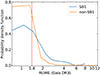 |
Fig. 13. Probability density function of Gaia DR3 RUWE for VELOCE SB1 and non-SB1 systems. |
Finally, we also investigated the Gaia astrometric quality indicators astrometric_gof_al and astrometric_excess_noise as indicators of multiplicity of Cepheids. However, no significant trends appeared in this comparison aside from a mild increase in astrometric_excess_noise near a sin i ∼ 1 au.
In summary, we find excess RUWE mainly for Cepheid binaries with projected semimajor axis close to 1 au. The parameter astrometric_excess_noise is also increased in this range, though the correlation is less clear. In addition to specific orbital configurations, elevated RUWE can arise from photocenter variations in unresolved binaries and in very bright stars, for example. Additionally, the majority of binary Cepheids are not identified by RUWE > 1.4.
5.4. Amplitude ratios as indicators of companion stars
Photometric amplitude ratios can be used to identify Cepheid companion stars in case the photometric contrast is sufficiently low (e.g. Madore 1977; Madore & Fernie 1980; Evans & Udalski 1994). Since most Cepheid companions are hot early-type stars, shorter-wavelength data is generally more sensitive to companions than longer-wavelength photometry. A noticeable exception are double-lined spectroscopic binaries (SB2) in the Large Magellanic Cloud that consist of a Cepheid and a giant companion (Pilecki et al. 2021).
In the Milky Way, Klagyivik & Szabados (2009) considered low ratios between photometric and RV amplitudes as an indicator for the presence of companion stars. Thanks to Gaia’s multiband photometry, such a comparison is possible here using a large sample of stars. Figure 14 thus shows the ratio between Gaia photometric and VELOCE RV amplitudes in three bands (GBp, G, and GRp) as a function of the logarithmic pulsation period. The higher ratios at shorter wavelength are readily explained by the larger photometric amplitudes. SB1 Cepheids identified in VELOCE are shown as filled circles, and stars which are not SB1 systems are shown as open circles. As a consequence of the Cepheid period-color relation, the contrast between Cepheid and companion should increase toward longer periods, rendering photometric detection more difficult. Additionally, any signal in the amplitude ratio should be enhanced at shorter wavelengths. However, the comparison between SB1 Cepheids and all others observed in all three bands reveals no indication that bona fide SB1 Cepheids have reduced amplitudes compared to other Cepheids (Figure 14). The only potential signature is a slightly reduced range of amplitude ratios for SB1 Cepheids, which, however, clusters in the center of the distribution. The comparison between photometric amplitudes in GBp vs GRp (not shown) yields the same impression. Hence, we find that Gaia’s photometric amplitudes are not good indicators of Cepheid companions.
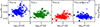 |
Fig. 14. Photometric amplitude ratios as indicators of companion stars. First three panels from left to right: photometric-to-RV amplitude ratios from Gaia DR3 and VELOCE against the logarithmic pulsation period, with wavelength of the photometric band increasing from left to right. Right panel: ratio of Gaia photometric amplitudes in GBp to GRp. Filled circles show SB1 Cepheids reported in VELOCE. Other single-mode Cepheids observed by VELOCE are shown as open circles. There is no clear difference between SB1 Cepheids and all others in any of the amplitudes considered, nor a dependence of such a difference on log Ppuls. |
6. Discussion and summary
We have presented the largest homogeneous investigation of 76 SB1 Cepheids to date based on the unprecedented RV data set provided by the VELOCE project (Paper I). An additional 14 SB1 candidates have been identified in Paper I, but are not discussed here due to their nature as candidate binaries. VELOCE data allow us to extend the search for binary Cepheids to fainter magnitudes, adding 32 new SB1 systems, and 18 first orbital determinations of Cepheids, 11 of which are fainter than mV > 8 mag (cf. Figure 9). Thanks to these improvements, we sharpened the uncertainty on the SB1 fraction of Cepheids by a factor of ∼2.3.
We present 30 definitive and three tentative orbital solutions, which range from the discovery of the shortest Porb in the Milky Way for R Cru (238 d) to ∼17 yr (AX Cir), and also include a correction to the orbital solution of δ Cep. For 18 Cepheids, we estimate orbital solutions for the first time. VELOCE observations are particularly sensitive to Porb ≲ 5 yr, and the available temporal baselines differ from star to star. The ensemble of orbital solutions suggests two peculiar features in the e − log(P) diagram, which are a possible exclusion zone of low-eccentricity systems (0 ≤ e < 0.2) at long orbital periods (Porb ≳ 10 yr) as well as a dearth of stars with orbital period in the range of 2.5 − 3.5 yr. Further observations and a more detailed analysis of detection limits will be needed to confirm these features.
Based on our search for SB1 Cepheids and a detailed investigation of evidence of orbital signals using literature, we find a SB1 fraction of 29.6 ± 3.4%. This is a lower limit since 14 SB1 candidates reported in Paper I were not considered in this fraction. Furthermore, we estimate the fraction of SB1 Cepheids with Porb < 10 yr of 15.2 ± 2.4%, half of which have Porb of less than 2.5 years. Our binary fraction estimates agree with previous reports, albeit with 2 − 3× lower uncertainty. Of course, SB1 Cepheids are detectable mainly for orbital periods of < 100 yr, and other methods must be considered to estimate the total binary fraction of Cepheids. Considerable effort is currently underway to comprehensively determine the binary fraction of Cepheids, employing a diverse array of techniques such as astrometry, spectroscopy, interferometry, and observations across various wavelengths. For example, Evans et al. (2022) estimated a total binary fraction of 57 ± 12% based on SB1 Cepheids, and Cepheids with evidence of companions from X-ray and UV observations. It is worth noting that future Gaia data releases, particularly DR4 and DR5, will contribute significantly with an abundance of astrometric orbits, enriching our understanding of these systems even further.
Several of the SB1 Cepheids studied here are part of triple systems, including AW Per (Evans et al. 2000), FF Aql (Udalski & Evans 1993), S Sge (Evans et al. 1993), V1334 Cyg (Abt & Levy 1970; Evans 1994), V0659 Cen (Evans et al. 2013, 2022), and W Sgr (Evans et al. 2009). Here, we further identify FO Car, RV Sco, RY Sco, and UX Per as triple systems with an inner SB1 and outer visual companion. Comparing the binary fraction and incidence of triples among Cepheids with dynamical NBODY simulations that assume an initial binary fraction of 100% (Dinnbier et al. 2024) suggests that a significant fraction of Cepheid progenitors (B-type stars) must be formed as triples or even higher-order systems.
Last, but not least, we find that the Gaia DR3 parallax quality indicator RUWE is elevated for Cepheid binaries whose projected semimajor axis, a sin i, is close to 1 au. However, upon assessing RUWE for both SB1 and non-SB1 from VELOCE, we ascertain that Gaia RUWE is not a reliable indicator for identifying Cepheid spectroscopic binaries and can be noticeably affected by photometric systematics, such as marginally resolved binaries or high apparent brightness. Additionally, RUWE tends to be slightly higher for Cepheids than for non-variable stars.
An examination of PMa in relation to various orbital properties of our stars does not reveal any correlation between the orbital orientation and PMa detection. Furthermore, all VELOCE Cepheids with previously reported PMa detections are also identified to be SB1 systems.
Precision radial velocities provide the most sensitive diagnostic of multiplicity of Cepheids to date. Future Gaia data releases will allow us to determine systemic masses of Cepheids using the combined astrometric and spectroscopic orbital signals. In Gaia DR3, only one Cepheid was reported with a non-single-star astrometric solution. Suspiciously, the orbital period of RX Cam was given as 33 months, matching exactly the observational baseline of Gaia DR3. However, RX Cam was unfortunately not observed as part of the VELOCE project. The upcoming fourth Gaia data release in combination with VELOCE data will be a treasure trove for determining accurate Cepheid masses and to establish a well-sampled mass-luminosity relation required to elucidate the physics of Cepheids, notably with respect to mixing processes, such as convection and rotation, required to explain the mass discrepancy problem (e.g. Prada Moroni et al. 2012; Anderson 2014).
Data availability
Supplementary material is available at https://zenodo.org/records/12818503
Defined for all VELOCE stars such that ϕ = 0 coincides with vγ on the steeper descending branch of the RV curve close to the mean observing date.
In the case of uniform priors, the MAP method coincides with the more known Maximum Likelihood Estimate (MLE) method.
These zero-points were established based on stars with stable vγ, more details can be found in Section 5.2 of Paper I.
In the supporting on-line material we have provided a table with the PMa binary flags from Kervella et al. (2022) for all stars in common with our sample.
Specifically, the Gaia DR3 astrometric parameters astrometric_gof_al = 31, astrometric_chi2_al = 41802, astrometric_excess_noise = 1.23, astrometric_gof_noise_sig = 1777, and RUWE = 2.7 all indicate the presence of unmodeled signal.
Zhou 2010 credited Szabados 1996 with detecting such evidence. Although FO Car is not listed in this publication, FR Car is, and we surmise a typo in Zhou 2010.
The RV dataset of SU Cyg is listed in the supplementary m aterial at: https://zenodo.org/records/12818503.
Acknowledgments
RIA, SS, and GV acknowledge support from the European Research Council (ERC) under the European Union’s Horizon 2020 research and innovation programme (Grant Agreement No. 947660). RIA, and SS further acknowledge support through a Swiss National Science Foundation Eccellenza Professorial Fellowship (award PCEFP2_194638). SS would further like to extend their acknowledgement to the Research Foundation-Flanders (grant number: 1239522N). This work has made use of data from the European Space Agency (ESA) mission Gaia (https://www.cosmos.esa.int/gaia), processed by the Gaia Data Processing and Analysis Consortium (DPAC, https://www.cosmos.esa.int/web/gaia/dpac/consortium). Funding for the DPAC has been provided by national institutions, in particular the institutions participating in the Gaia Multilateral Agreement. The lead authors would like to acknowledge the very useful compilation of information on binary Cepheids provided by Laszlo Szabados at Konkoly Observatory (Szabados 2003, https://cep.konkoly.hu/intro.html).
References
- Abt, H. A., & Levy, S. G. 1970, PASP, 82, 334 [NASA ADS] [CrossRef] [Google Scholar]
- Anderson, R. I. 2013, Ph.D. Thesis, Université de Genève, Switzerland [Google Scholar]
- Anderson, R. I. 2014, A&A, 566, L10 [NASA ADS] [CrossRef] [EDP Sciences] [Google Scholar]
- Anderson, R. I. 2016, MNRAS, 463, 1707 [NASA ADS] [CrossRef] [Google Scholar]
- Anderson, R. I. 2019, A&A, 623, A146 [NASA ADS] [CrossRef] [EDP Sciences] [Google Scholar]
- Anderson, R. I. 2020, in Proceedings of the Conference Stars and their Variability Observed from Space, eds. C. Neiner, W. W. Weiss, D. Baade, et al., 61 [Google Scholar]
- Anderson, R. I., & Riess, A. G. 2018, ApJ, 861, 36 [NASA ADS] [CrossRef] [Google Scholar]
- Anderson, R. I., Eyer, L., & Mowlavi, N. 2013, MNRAS, 434, 2238 [Google Scholar]
- Anderson, R. I., Sahlmann, J., Holl, B., et al. 2015, ApJ, 804, 144 [CrossRef] [Google Scholar]
- Anderson, R. I., Casertano, S., Riess, A. G., et al. 2016a, ApJS, 226, 18 [NASA ADS] [CrossRef] [Google Scholar]
- Anderson, R. I., Saio, H., Ekström, S., Georgy, C., & Meynet, G. 2016b, A&A, 591, A8 [NASA ADS] [CrossRef] [EDP Sciences] [Google Scholar]
- Anderson, R. I., Mérand, A., Kervella, P., et al. 2016c, MNRAS, 455, 4231 [Google Scholar]
- Anderson, R. I., Viviani, G., Shetye, S. S., et al. 2024, A&A, 686, A177 [NASA ADS] [CrossRef] [EDP Sciences] [Google Scholar]
- Arellano-Ferro, A., & Madore, B. F. 1985, The Observatory, 105, 207 [NASA ADS] [Google Scholar]
- Babel, J., Burki, G., Mayor, M., Chmielewski, Y., & Waelkens, C. 1989, A&A, 216, 125 [NASA ADS] [Google Scholar]
- Barnes, T. G., III, Moffett, T. J., & Slovak, M. H. 1987, ApJS, 65, 307 [NASA ADS] [CrossRef] [Google Scholar]
- Barnes, T. G., III, Jeffery, E. J., Montemayor, T. J., & Skillen, I. 2005, ApJS, 156, 227 [NASA ADS] [CrossRef] [Google Scholar]
- Belokurov, V., Penoyre, Z., Oh, S., et al. 2020, MNRAS, 496, 1922 [Google Scholar]
- Benedict, G. F., Barnes, T. G., Evans, N. R., et al. 2022, AJ, 163, 282 [NASA ADS] [CrossRef] [Google Scholar]
- Bersier, D. 2002, ApJS, 140, 465 [NASA ADS] [CrossRef] [Google Scholar]
- Bersier, D., Burki, G., Mayor, M., & Duquennoy, A. 1994, A&AS, 108, 25 [NASA ADS] [Google Scholar]
- Binnenfeld, A., Shahaf, S., Anderson, R. I., & Zucker, S. 2022, A&A, 659, A189 [NASA ADS] [CrossRef] [EDP Sciences] [Google Scholar]
- Borgniet, S., Kervella, P., Nardetto, N., et al. 2019, A&A, 631, A37 [NASA ADS] [CrossRef] [EDP Sciences] [Google Scholar]
- Breitfelder, J., Mérand, A., Kervella, P., et al. 2016, A&A, 587, A117 [CrossRef] [EDP Sciences] [Google Scholar]
- Burki, G., Mayor, M., & Benz, W. 1982, A&A, 109, 258 [NASA ADS] [Google Scholar]
- Caputo, F., Bono, G., Fiorentino, G., Marconi, M., & Musella, I. 2005, ApJ, 629, 1021 [CrossRef] [Google Scholar]
- Coulson, I. M., & Caldwell, J. A. R. 1985, SAAO Circ., 9, 5 [NASA ADS] [Google Scholar]
- Csörnyei, G., Szabados, L., Molnár, L., et al. 2022, MNRAS, 511, 2125 [CrossRef] [Google Scholar]
- Dinnbier, F., Anderson, R. I., & Kroupa, P. 2024, A&A, in press, https://doi.org/10.1051/0004-6361/202347641 [NASA ADS] [CrossRef] [EDP Sciences] [Google Scholar]
- Ekström, S., Georgy, C., Eggenberger, P., et al. 2012, A&A, 537, A146 [Google Scholar]
- Evans, N. R. 1988, ApJS, 66, 343 [NASA ADS] [CrossRef] [Google Scholar]
- Evans, N. R. 1991, ApJ, 372, 597 [NASA ADS] [CrossRef] [Google Scholar]
- Evans, N. R. 1992, ApJ, 384, 220 [NASA ADS] [CrossRef] [Google Scholar]
- Evans, N. R. 1994, ApJ, 436, 273 [NASA ADS] [CrossRef] [Google Scholar]
- Evans, N. R. 1995, ApJ, 445, 393 [NASA ADS] [CrossRef] [Google Scholar]
- Evans, N. R. 2000, AJ, 119, 3050 [NASA ADS] [CrossRef] [Google Scholar]
- Evans, N. R., & Lyons, R. W. 1994, AJ, 107, 2164 [NASA ADS] [CrossRef] [Google Scholar]
- Evans, N. R., & Udalski, A. 1994, AJ, 108, 653 [NASA ADS] [CrossRef] [Google Scholar]
- Evans, N. R., Szabados, L., & Udalska, J. 1990, PASP, 102, 981 [NASA ADS] [CrossRef] [Google Scholar]
- Evans, N. R., Arellano Ferro, A., & Udalska, J. 1992, AJ, 103, 1638 [NASA ADS] [CrossRef] [Google Scholar]
- Evans, N. R., Welch, D. L., Slovak, M. H., Barnes, T. G., III, & Moffett, T. J. 1993, AJ, 106, 1599 [NASA ADS] [CrossRef] [Google Scholar]
- Evans, N. R., Vinko, J., & Wahlgren, G. M. 2000, AJ, 120, 407 [NASA ADS] [CrossRef] [Google Scholar]
- Evans, N. R., Massa, D., & Proffitt, C. 2009, AJ, 137, 3700 [NASA ADS] [CrossRef] [Google Scholar]
- Evans, N. E., Bond, H. E., Schaefer, G. H., et al. 2013, AJ, 146, 93 [NASA ADS] [CrossRef] [Google Scholar]
- Evans, N. R., Berdnikov, L., Lauer, J., et al. 2015, AJ, 150, 13 [NASA ADS] [CrossRef] [Google Scholar]
- Evans, N. R., Günther, H. M., Bond, H. E., et al. 2020, ApJ, 905, 81 [CrossRef] [Google Scholar]
- Evans, N. R., Engle, S., Pillitteri, I., et al. 2022, ApJ, 938, 153 [NASA ADS] [CrossRef] [Google Scholar]
- Ford, E. B. 2005, AJ, 129, 1706 [Google Scholar]
- Ford, E. B. 2006, ApJ, 642, 505 [Google Scholar]
- Foreman-Mackey, D., Hogg, D. W., Lang, D., & Goodman, J. 2013, PASP, 125, 306 [Google Scholar]
- Fulton, B. J., Petigura, E. A., Blunt, S., & Sinukoff, E. 2018, PASP, 130, 044504 [Google Scholar]
- Gaia Collaboration (Prusti, T., et al.) 2016a, A&A, 595, A1 [NASA ADS] [CrossRef] [EDP Sciences] [Google Scholar]
- Gaia Collaboration (Brown, A. G. A., et al.) 2016b, A&A, 595, A2 [NASA ADS] [CrossRef] [EDP Sciences] [Google Scholar]
- Gaia Collaboration (Brown, A. G. A., et al.) 2018, A&A, 616, A1 [NASA ADS] [CrossRef] [EDP Sciences] [Google Scholar]
- Gaia Collaboration (Brown, A. G. A., et al.) 2021, A&A, 649, A1 [NASA ADS] [CrossRef] [EDP Sciences] [Google Scholar]
- Gaia Collaboration (Arenou, F., et al.) 2023, A&A, 674, A34 [CrossRef] [EDP Sciences] [Google Scholar]
- Gallenne, A., Monnier, J. D., Mérand, A., et al. 2013, A&A, 552, A21 [CrossRef] [EDP Sciences] [Google Scholar]
- Gallenne, A., Kervella, P., Mérand, A., et al. 2014a, in Precision Asteroseismology, eds. J. A. Guzik, W. J. Chaplin, G. Handler, & A. Pigulski, 301, 411 [NASA ADS] [Google Scholar]
- Gallenne, A., Mérand, A., Kervella, P., et al. 2014b, A&A, 561, L3 [NASA ADS] [CrossRef] [EDP Sciences] [Google Scholar]
- Gallenne, A., Mérand, A., Kervella, P., et al. 2015, A&A, 579, A68 [NASA ADS] [CrossRef] [EDP Sciences] [Google Scholar]
- Gallenne, A., Mérand, A., Kervella, P., et al. 2016, MNRAS, 461, 1451 [NASA ADS] [CrossRef] [Google Scholar]
- Gallenne, A., Kervella, P., Evans, N. R., et al. 2018, ApJ, 867, 121 [Google Scholar]
- Gallenne, A., Kervella, P., Borgniet, S., et al. 2019, A&A, 622, A164 [NASA ADS] [CrossRef] [EDP Sciences] [Google Scholar]
- Genovali, K., Lemasle, B., Bono, G., et al. 2014, A&A, 566, A37 [NASA ADS] [CrossRef] [EDP Sciences] [Google Scholar]
- Gieren, W. 1982, ApJS, 49, 1 [NASA ADS] [CrossRef] [Google Scholar]
- Gieren, W. P. 1985, ApJ, 295, 507 [NASA ADS] [CrossRef] [Google Scholar]
- Gorynya, N. A., Irsmambetova, T. R., Rastorgouev, A. S., & Samus, N. N. 1992, Sov. Astron. Lett., 18, 316 [NASA ADS] [Google Scholar]
- Gorynya, N. A., Rastorguev, A. S., & Samus, N. N. 1996a, Astron. Lett., 22, 33 [NASA ADS] [Google Scholar]
- Gorynya, N. A., Samus’, N. N., Rastorguev, A. S., & Sachkov, M. E. 1996b, Astron. Lett., 22, 175 [Google Scholar]
- Griffin, R. F. 2016, The Observatory, 136, 209 [Google Scholar]
- Groenewegen, M. A. T. 2008, A&A, 488, 25 [NASA ADS] [CrossRef] [EDP Sciences] [Google Scholar]
- Hertzsprung, E. 1913, Astron. Nachr., 196, 201 [NASA ADS] [Google Scholar]
- Hilditch, R. W. 2001, An Introduction to Close Binary Stars (Cambridge: Cambridge University Press) [Google Scholar]
- Hintz, E. G., Harding, T. B., & Hintz, M. L. 2021, AJ, 162, 149 [NASA ADS] [CrossRef] [Google Scholar]
- Imbert, M. 1984, A&AS, 58, 529 [NASA ADS] [Google Scholar]
- Karczmarek, P., Smolec, R., Hajdu, G., et al. 2022, ApJ, 930, 65 [NASA ADS] [CrossRef] [Google Scholar]
- Kervella, P., Arenou, F., Mignard, F., & Thévenin, F. 2019a, A&A, 623, A72 [NASA ADS] [CrossRef] [EDP Sciences] [Google Scholar]
- Kervella, P., Gallenne, A., Remage Evans, N., et al. 2019b, A&A, 623, A116 [NASA ADS] [CrossRef] [EDP Sciences] [Google Scholar]
- Kervella, P., Arenou, F., & Thévenin, F. 2022, A&A, 657, A7 [NASA ADS] [CrossRef] [EDP Sciences] [Google Scholar]
- Khan, S., Anderson, R. I., Miglio, A., Mosser, B., & Elsworth, Y. P. 2023, A&A, 680, A105 [NASA ADS] [CrossRef] [EDP Sciences] [Google Scholar]
- Kiss, L. L. 1998, MNRAS, 297, 825 [NASA ADS] [CrossRef] [Google Scholar]
- Kiss, L. L., & Bedding, T. R. 2005, MNRAS, 358, 883 [NASA ADS] [CrossRef] [Google Scholar]
- Klagyivik, P., & Szabados, L. 2009, A&A, 504, 959 [NASA ADS] [CrossRef] [EDP Sciences] [Google Scholar]
- Kovtyukh, V., Szabados, L., Chekhonadskikh, F., Lemasle, B., & Belik, S. 2015, MNRAS, 448, 3567 [NASA ADS] [CrossRef] [Google Scholar]
- Kovtyukh, V., Lemasle, B., Bono, G., et al. 2022, MNRAS, 510, 1894 [Google Scholar]
- Leavitt, H. S., & Pickering, E. C. 1912, Harv. Coll. Obs. Circ., 173, 1 [Google Scholar]
- Lindegren, L. 2018, Re-normalising the Astrometric Chi-square in Gaia DR2 (Lund Observatory) [Google Scholar]
- Lindegren, L., Hernández, J., Bombrun, A., et al. 2018, A&A, 616, A2 [NASA ADS] [CrossRef] [EDP Sciences] [Google Scholar]
- Lindegren, L., Klioner, S. A., Hernández, J., et al. 2021, A&A, 649, A2 [EDP Sciences] [Google Scholar]
- Lloyd Evans, T. 1968, MNRAS, 141, 109 [NASA ADS] [CrossRef] [Google Scholar]
- Lloyd Evans, T. 1980, SAAO Circ., 1, 257 [NASA ADS] [Google Scholar]
- Lloyd Evans, T. 1982, MNRAS, 199, 925 [NASA ADS] [Google Scholar]
- Luck, R. E., & Lambert, D. L. 2011, AJ, 142, 136 [Google Scholar]
- Madore, B. F. 1977, MNRAS, 178, 505 [CrossRef] [Google Scholar]
- Madore, B. F., & Fernie, J. D. 1980, PASP, 92, 315 [NASA ADS] [CrossRef] [Google Scholar]
- Michalik, D., Lindegren, L., & Hobbs, D. 2015, A&A, 574, A115 [NASA ADS] [CrossRef] [EDP Sciences] [Google Scholar]
- Mochejska, B. J., Macri, L. M., Sasselov, D. D., & Stanek, K. Z. 2000, AJ, 120, 810 [NASA ADS] [CrossRef] [Google Scholar]
- Molnár, L., Derekas, A., Szabó, R., et al. 2017, MNRAS, 466, 4009 [Google Scholar]
- Moore, J. H. 1929, PASP, 41, 56 [Google Scholar]
- Nardetto, N., Hocdé, V., Kervella, P., et al. 2024, A&A, 684, L9 [NASA ADS] [CrossRef] [EDP Sciences] [Google Scholar]
- Neilson, H. R., Schneider, F. R. N., Izzard, R. G., Evans, N. R., & Langer, N. 2015, A&A, 574, A2 [NASA ADS] [CrossRef] [EDP Sciences] [Google Scholar]
- Perryman, M. A. C., Lindegren, L., Kovalevsky, J., et al. 1997, A&A, 323, L49 [Google Scholar]
- Petterson, O. K. L., Cottrell, P. L., & Albrow, M. D. 2004, MNRAS, 350, 95 [NASA ADS] [CrossRef] [Google Scholar]
- Pilecki, B., Pietrzyński, G., Anderson, R. I., et al. 2021, ApJ, 910, 118 [NASA ADS] [CrossRef] [Google Scholar]
- Poggio, E., Drimmel, R., Cantat-Gaudin, T., et al. 2021, A&A, 651, A104 [NASA ADS] [CrossRef] [EDP Sciences] [Google Scholar]
- Pont, F., Mayor, M., & Burki, G. 1994, A&A, 285, 415 [NASA ADS] [Google Scholar]
- Prada Moroni, P. G., Gennaro, M., Bono, G., et al. 2012, ApJ, 749, 108 [NASA ADS] [CrossRef] [Google Scholar]
- Proust, D., Ochsenbein, F., & Pettersen, B. R. 1981, A&AS, 44, 179 [NASA ADS] [Google Scholar]
- Queloz, D., Mayor, M., Udry, S., et al. 2001, The Messenger, 105, 1 [NASA ADS] [Google Scholar]
- Raskin, G., van Winckel, H., Hensberge, H., et al. 2011, A&A, 526, A69 [CrossRef] [EDP Sciences] [Google Scholar]
- Riess, A. G., Casertano, S., Yuan, W., et al. 2018, ApJ, 861, 126 [NASA ADS] [CrossRef] [Google Scholar]
- Russo, G., Sollazzo, C., & Coppola, M. 1981, A&A, 102, 20 [NASA ADS] [Google Scholar]
- Shetye, S. 2022, Video Memorie della Societa Astronomica Italiana, 2, 20 [NASA ADS] [Google Scholar]
- Stassun, K. G., & Torres, G. 2021, ApJ, 907, L33 [NASA ADS] [CrossRef] [Google Scholar]
- Stepien, K. 1968, Acta Astron., 18, 537 [NASA ADS] [Google Scholar]
- Storm, J., Carney, B. W., Gieren, W. P., et al. 2004, A&A, 415, 531 [NASA ADS] [CrossRef] [EDP Sciences] [Google Scholar]
- Szabados, L. 1989, Commun. Konkoly Obs. Hung., 94, 1 [NASA ADS] [Google Scholar]
- Szabados, L. 1992, The Observatory, 112, 57 [NASA ADS] [Google Scholar]
- Szabados, L. 1996, A&A, 311, 189 [NASA ADS] [Google Scholar]
- Szabados, L. 2003, IBVS, 5394, 1 [NASA ADS] [Google Scholar]
- Szabados, L., & Pont, F. 1998, A&AS, 133, 51 [NASA ADS] [CrossRef] [EDP Sciences] [Google Scholar]
- Szabados, L., Derekas, A., Kiss, L. L., et al. 2013a, MNRAS, 430, 2018 [NASA ADS] [CrossRef] [Google Scholar]
- Szabados, L., Anderson, R. I., Derekas, A., et al. 2013b, MNRAS, 434, 870 [NASA ADS] [CrossRef] [Google Scholar]
- Szabados, L., Cseh, B., Kovács, J., et al. 2014, MNRAS, 442, 3155 [CrossRef] [Google Scholar]
- Szatmary, K. 1990, J. Am. Assoc. Var. Star Obs., 19, 52 [NASA ADS] [Google Scholar]
- Torres, G. 2023, MNRAS, 526, 2510 [NASA ADS] [CrossRef] [Google Scholar]
- Turner, D. G., Bryukhanov, I. S., Balyuk, I. I., et al. 2007, PASP, 119, 1247 [NASA ADS] [CrossRef] [Google Scholar]
- Udalski, A., & Evans, N. R. 1993, AJ, 106, 348 [NASA ADS] [CrossRef] [Google Scholar]
- Vinko, J. 1991, Ap&SS, 183, 17 [NASA ADS] [CrossRef] [Google Scholar]
- Virtanen, P., Gommers, R., Oliphant, T. E., et al. 2020, Nat. Meth., 17, 261 [Google Scholar]
- Wahlgren, G. M., & Evans, N. R. 1998, A&A, 332, L33 [NASA ADS] [Google Scholar]
- Wilson, T. D., Carter, M. W., Barnes, T. G., III, van Citters, G. W., & Moffett, T. J. 1989, ApJS, 69, 951 [NASA ADS] [CrossRef] [Google Scholar]
- Zhou, A. Y. 2010, ArXiv e-prints [arXiv:1002.2729] [Google Scholar]
Appendix A: Guiding camera Image
When available, the Coralie and Hermes guiding camera images were utilized to examine for triple systems. In Figure A.1, we present a guiding camera image of FO Car obtained from Coralie.
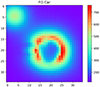 |
Fig. A.1. Coralie guiding camera image of FO Car. The center of the Cepheid is dark because of the fiber placement during the integration. The object at the top left is an outer (visual) companion, which renders the SB1 Cepheid FO Car a triple system. |
Appendix B: Notes on individual binaries
We have presented evidence of the SB1 nature of 76 Milky Way Cepheids on timescales spanning up to 40 years, including 32 stars whose SB1 nature was not previously known. The following provides additional background for specific stars of interest, notably if our results disagree with previous studies. We note that several Cepheids were first reported to be SB1 systems based on early VELOCE results, such as FN Vel and MU Cep (Anderson 2013), BG Vel and RZ Vel (Szabados et al. 2013b), δ Cep (Anderson et al. 2015), and AQ Car, CD Cyg, KN Cen, SS CMa, SZ Cyg, XZ Car, VY Car and X Pup (Anderson et al. 2016a). Anderson et al. (2016a) noticed tentative evidence of vγ variations in VY Car, AQ Car, SZ Cyg and X Pup. However, they ultimately deemed these findings inconclusive due to imprecise data in the literature and the occasional substantial fluctuations in pulsational variability. In the current work we successfully detect these vγ variations for SZ Cyg (when VELOCE data is combined with zero-point corrected literature datasets, see Figure 8) and AQ Car (cf. Table 5, Figure B.1). Nevertheless, in the case of VY Car and X Pup, the vγ values, when adjusted for zero-point, do not reveal any consistent variation indicative of binarity (see Section 4 in the supplementary m aterial).
α UMi (Polaris) was one of the first Cepheids whose nature as an SB1 system was realized (Moore 1929), and much literature exists on this star. Polaris was extensively studied using pre-2019 VELOCE data by Anderson (2019), who determined a full orbital solution and studied the stability of RV amplitudes as well as the presence of additional periodic signals. Given the very long ∼30-year orbital period, we did not update the orbital solution here and instead refer to the aforementioned publication as well as Torres (2023) for orbital parameters.
δ Cephei is the archetype of classical Cepheids and was discovered to be an SB1 system using an earlier subset of VELOCE data. Anderson et al. (2015) estimated an orbit with  d,
d,  km s−1, and
  by combining new RV data with RV measurements from the literature. A main difficulty of this approach was the correction of zero-point differences for datasets with short (∼1 yr) baselines. Here, we report a correction to the orbital solution, with Porb = 3450.9 ± 19.6 d, K = 3.01 ± 0.02 km s−1, and e = 0.745 ± 0.006, based purely on VELOCE data and hence not subject to the uncertainties associated with literature zero-point offsets. This updated orbit of δ Cep was already presented at the 2022 RR Lyr-Cep conference in La Palma (Shetye 2022). It agrees reasonably well with the results recently presented by Nardetto et al. (2024) based on a combination of High Accuracy Radial velocity Planet Searcher for the Northern hemisphere (HARPS-N) data and existing literature. Their estimated orbital period of 3401.8 d and eccentricity of 0.71 differ by 2−σ and 1.7−σ from ours. These small differences may result from their use of a heterogeneous dataset, or the better coverage of the periastron passage by the HARPS-N data. As Figure 2 shows, the orbit is now completely sampled and contained within the VELOCE baseline (3620 d). Importantly, the extreme ends of the orbital velocity have been observed and tightly constrain e and K. Unfortunately, including literature data for a V+L orbit does not improve the orbital solution due to the same issues that affected the prior analysis. Extending the baseline with future Hermes observations will further improve the orbital period. We note that the mass function and the high brightness contrast imply the companion to be a low-mass star, possibly a white dwarf (Gallenne et al. 2016). A similar deduction was made in the recent X-ray study of Cepheids by Evans et al. (2022). A companion of G spectral type or later would be expected to be detected in X-rays, which puts a lower limit on the mass of the companion. Finally, we note that the single-star astrometric solution provided in Gaia DR3 clearly indicates poor fit quality8. It thus appears likely that Gaia’s next data release could deliver an astrometric orbital solution, as predicted by Anderson et al. (2015).
η Aql was recently studied by Benedict et al. (2022) using spectroscopic, photometric and astrometric (from the Hubble Space Telescope (HST) Fine Guidance Sensor) observations, including unpublished VELOCE data. No significant variations in the RV residuals were detected after removing the Cepheid pulsational RV signature, leading Benedict et al. (2022) to conclude that either η Aql has a very long orbital period (longer than their baseline of ∼38 years) or that it has a face-on orbit. We considered an extended temporal baseline by including RV data from Lloyd Evans (1980), Barnes et al. (1987), and Wilson et al. (1989) and detect a 3-σ variation in the Δvγ (Figure 8). If the older datasets are to be believed despite large RV uncertainties of ∼1 km s−1, then η Aql is indeed an SB1 Cepheid with a very long orbit of more than 50 years. Verifying whether this spectroscopic companion corresponds to the one identified in the UV imaging and spectra of η Aql by Evans et al. (2013), at a separation of 180 au, necessitates a follow-up of the long orbital period.
AQ Car was reported to show tentative signs of time-variable vγ using an earlier set of VELOCE and literature data. In Paper I, we confirmed the SB1 nature of this star. Although weak, ∼0.7 km s−1, the signal is clearly present in the VELOCE data thanks to the baseline of ∼4 yr. Although literature datasets appear imprecise to usefully inform the vγ variations (cf. Figure B.1), in actuality, the fluctuations observed in the literature data surpass a 3-σ threshold. As σ is calculated using VELOCE data under the assumption of no orbital motion, consequently, the deviations from a stable vγ are consistently underestimated in this scenario.
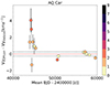 |
Fig. B.1. Temporal variation of vγ for AQ Car based on RVTF. The data points after BJD > 56000 are from VELOCE. |
AQ Pup was reported to have a photometric companion (Evans & Udalski 1994) that was not previously confirmed spectroscopically (Vinko 1991). Here, we report low-amplitude vγ variations (∼ 3.3 km s−1) on a timescale of 2500 days. Whether this signature corresponds to the photometric companion remains unclear.
ASAS J064540+0330.4 – We present the first orbital fit for ASAS J064540+0330.4 with a Porb of 901.18 ± 2.81 days and an eccentricity of 0.44 ± 0.01. The pulsational residuals of ASAS J064540+0330.4 indicate additional signals beyond the orbital ones. It is important to note that further observational follow-up is necessary to sample the orbital phase better and establish this orbit more firmly. The combined orbital and pulsational fit can be found in the supplementary m aterial.
ASAS J103158-5814.7 (GDR3 5351436724362450304) is a particularly interesting star, cf. Figure B.2 and Paper I. It exhibits three signals at once: very short-period overtone pulsation (classified as first overtone by Gaia DR3 SOS, Ppuls = 1.11936 d), high-amplitude orbital motion exceeding 13 km s−1, cf. Table 5, and strongly modulated pulsation amplitudes reminiscent of the “Blazhko" Cepheid V0473 Lyrae (Burki et al. 1982; Molnár et al. 2017). At present, the orbital variations do not allow the estimation of an orbital period and we will thus continue monitoring this intriguing star. Unfortunately, this star was not included in the list of Cepheids with time-series RV data in Gaia DR3.
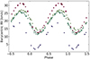 |
Fig. B.2. Phase-folded Coralie RV of ASASJ103158-5814.7, the same star that exhibits orbital motion, the variable amplitude, and a variable pulsation period. |
AX Cir is a known SB1 and its orbit was first derived by Petterson et al. (2004). Our Porb estimate of ∼6285 days differs by 5% (10-σ) from that of Petterson et al. (2004). While our combined dataset, comprising VELOCE and literature data, incompletely samples orbital phases, we obtain an eccentricity that is in total agreement with the previously reported orbital eccentricity for AX Cir.
FN Vel was discovered to be an SB1 by Anderson (2013) who provided a first orbital solution. Kovtyukh et al. (2015) showed evidence of the companion using the Ca H & K lines. Here, we provide an updated orbital solution.
BP Cir is known to host a hot main-sequence companion (Arellano-Ferro & Madore 1985; Evans et al. 1992) based on IUE spectroscopy. Petterson et al. (2004) reported vγ variations exceeding 5 km s−1 and that the star could possibly have a long orbital period. Using VELOCE alone we have vγ variations of ∼2 km s−1, however, when we combined VELOCE with literature datasets from Petterson et al. (2004) and Borgniet et al. (2019) we found vγ variations of ∼ 4 km s−1 at a temporal baseline of 9000 days. We estimated BP Cir’s orbital period using VELOCE and literature datasets, and found a tentative solution with Porb ∼ 4300 days and e ∼ 0.8. Nevertheless, due to limitations in the available data, we are unable to definitively determine whether a period of 4300 days or twice that duration provides a more accurate representation.
FO Car’s observations began in March 2016, and we find a Keplerian orbit of Porb ∼ 1660 d. To the best of our knowledge, no previous publication9 has presented the case of FO Car. However, the online database of binary Cepheids (Szabados 2003) lists it as a spectroscopic binary, crediting Szabados & Berdnikov (in preparation). Russo et al. (1981) found photometric evidence of a companion using a phase shift technique involving optical and UV data. Based on the visual companion identified during the spectroscopic observations (cf. Figure A.1) we consider this as the most likely source of the phase shift. Given the angular separation, the visual companion is clearly not the cause of the 4.5 yr orbit, and hence, FO Car is a triple system composed of the Cepheid with an inner spectroscopic and outer visual companion.
MU Cep – The spectroscopic binarity of MU Cep (not to be confused with the much brighter red supergiant μ Cep) was discovered by Anderson (2013). Here we present an updated orbital solution. The previously reported Porb ∼ 1500 ± 350 d exceeded the observational baseline. Thanks to continued follow-up of this faint star (⟨mV⟩ = 12.3 mag), we have achieved nearly complete coverage of MU Cep’s orbital phase and obtain tight orbital constraints, with Porb = 2028 ± 2.7 d.
R Cru is listed as an SB1 in the database by Szabados (2003), which credits unpublished work by L. Szabados and D. Bersier with this discovery. More recently, Evans et al. (2020) reported a visual companion of R Cru at a separation of 1.9 arcseconds based on HST imaging. We have acquired nearly 7 yr worth of very high-precision RV data for this bright Cepheid. The data clearly reveal low-amplitude orbital motion with Porb ∼ 238 d, rendering R Cru the Cepheid with the shortest orbital period in the Milky Way. The template fitting routine further finds evidence of nonlinear period changes (see Figure 15 of Paper I), cf. also Csörnyei et al. (2022). The relative semimajor axis of arel > 274 R⊙ implies that the Cepheid and its companion are not in contact, assuming a Cepheid radius of 47 R⊙ computed using a P-R relation (Anderson et al. 2016b) and a nearly circular orbit. For a Cepheid mass of around 5 M⊙ and a 2 M⊙ A2 companion (upper limit from the IUE spectrum, Evans 1992), the mass function for a circular orbit yields a minimum inclination of > 3.3 deg, improving slightly over the limit from the mass function alone (1.6 deg). For the range of inclinations 3.3 − 90 deg, and assuming a 5 M⊙ Cepheid, we thus find the allowed mass range for the companion to be between 0.09 − 2.0 M⊙.
RV Sco – Proust et al. (1981) list RV Sco as a visual multiple system, with a non-variable companion of mV ∼ 13 mag at a separation of 6.0 arcseconds. Evans (1992) did not detect any photometric companion for RV Sco within their IUE spectral analysis. Szabados (1989) suspected its binarity through its variable γ-velocity. Here, we confirm the finding as we detected significant (Ap2p ∼ 5.3 km s−1) amplitude variation in RV resulting into a 4-σ detection of binarity. RV Sco is therefore a triple (SB1 + visual companion) system.
RY Sco is listed as a visual binary in Szabados (2003), with references to Proust et al. (1981), Evans & Udalski (1994). We here detect the stars’s SB1 nature for the first time, with very low-amplitude orbital RV variations of ∼0.6 km s−1. Combining VELOCE with literature datasets and extending to longer baseline, we notice a vγ variation of ∼2.5 km s−1 on a timescale of 41 years. RY Sco is thus most likely a triple system with both a visual and a spectroscopic companions.
RZ Vel was reported to be an SB1 Cepheid by Szabados et al. (2013b). Szabados et al. (2013b) used a subset of VELOCE data (between BJD 2455650 – 2456400). We extended this VELOCE baseline to BJD 2459600 and combined it with literature datasets from Lloyd Evans (1980), Coulson & Caldwell (1985), Bersier (2002), Borgniet et al. (2019). Although, data from Bersier (2002) was also included in Szabados et al. (2013b), we do not detect 3-σvγ variations for this or any other recent dataset after the year 2000.
S Mus was first identified as a binary using photometric observations (Lloyd Evans 1968). A first orbital solution was presented by Lloyd Evans (1982), with several others since. In particular, Petterson et al. (2004) provided a precise update to this solution, and Binnenfeld et al. (2022) determined the periodicity using partial periodograms directly computed from the spectra rather than RV measurements. We gathered 78 high-precision Coralie RVs over a total baseline of 6.3 yr. These data alone yield an orbital solution in agreement (to within 1 day) with Petterson et al. (2004) and Gallenne et al. (2019). As shown by Evans et al. (2015, 2020), the companion is an X-ray active B3V star.
S Nor was detected as an SB1 by Szabados (1989), where they estimated tentative orbital periods of 3300 or 6500 days. Groenewegen (2008) modeled S Nor’s RV data using a circular orbit with a fixed Porb of 3600 days and concluded that more RV data are needed to better determine this orbit. Here, we do not find this orbital estimate to be consistent with VELOCE data. We do not detect any vγ variations with VELOCE data alone, however, when VELOCE is combined with literature datasets we do obtain a 3-σ detection for the oldest RV datasets. However, the only cluster that exceeds 3-σ is based on only three observations and the uncertainty of this particular cluster is likely underestimated. Consequently, we doubt the validity of the only > 3-σ outlier and cannot consider the star a bonafide binary. Nevertheless, if the RVTF results are taken at face value, then the orbit would have to be significantly eccentric. Lastly, the vγ residuals indicate that a potential orbit clearly has high eccentricity.
SU Cyg is a solitary case wherein the pulsation model was derived using a combination of VELOCE data and zero-point corrected RV data from Borgniet et al. (2019). While VELOCE data provided strong constraints on the orbit, they were insufficient on their own to create a satisfactory Fourier series model. To address this, we included the Borgniet et al. (2019) measurements to formulate the RV template. This template was then used to compute vγ10. Finally, employing the MCMC method, we obtained the V+L orbit of SU Cyg with Porb of ∼548 ± 0.1 d and eccentricity of ∼0.34 ± 0.005. These orbital estimates are in agreement with ΔPorb < 1 d (all orbital elements within 3-σ difference) the ones in the literature from Evans (1988), Imbert (1984), Groenewegen (2008).
TX Mon was first reported as an SB1 by Szabados & Pont (1998), who estimated a short Porb ≈ 470 ± 30 d. We here confirm the SB1 nature of the star and determine the orbit, albeit at much longer Porb = 1607 ± 1 d, with K = 11.9 ± 0.04 km s−1.
V0659 Cen is host to a hot B6.0V companion detected directly using IUE UV spectroscopy (Evans 1994). V0659 Cen also has a high X-ray flux potentially originating from its companion (Evans et al. 2022). Here we present the first RV evidence of the Cepheid’s orbital motion with a peak-to-peak RV variation of ≳5 km s−1. Combining VELOCE and literature data, we estimate a preliminary orbital period Porb ∼ 9300 ± 130 d with mild eccentricity (e = 0.32). We designate this orbit as tentative due to the ambiguity regarding whether the orbital period is approximately 6000 or 9000 days. It should be emphasized that the current uncertainties, which are around 100 days, do not account for this ambiguity. Additional HST UV spectroscopy will be particularly valuable to measure the mass of the Cepheid (Evans et al. in prep.).
V1334 Cyg is among the few sample cases where there is a disagreement between V and V+L estimates, specifically of 0.8% (3-σ) in Porb for V1334 Cyg. Even after combining the VELOCE and literature datasets, constraints on the ascending part and extremities of the orbital phase remain limited. As the literature dataset from Gorynya et al. (1992) and Borgniet et al. (2019) add extra constraints on the descending branch of the orbital phase, we prefer the V+L orbital estimate for V1334 Cyg. Furthermore, both V and V+L orbital estimates are in 0.5% (3-σ) disagreement with the ones from Gallenne et al. (2018) and 3-σ and 2-σ, respectively, with the ones from Evans (2000). This maybe attributed to the aforementioned poor sampling at some orbital phases. Future observations, with overall improved sampling will help to elucidate the discrepancy. Lastly, Gallenne et al. (2018) demonstrated that Gaia DR2 parallax is off by 3.6-σ compared to the orbital parallax determined from the visual orbit + RVs of both components. This could be another reason for the discrepancy between our orbital parameters and the ones from Gallenne et al. (2018).
VY Car was considered a tentative SB1 candidate by Anderson et al. (2016a). Despite improved treatment of instrumental zero-point offsets, the orbital signal has neither disappeared nor clarified. We note the RVTF analysis suggests a trend with time. However, none of the epochs deviate from the average by more than 3-σ. Hence, VY Car remains an unconfirmed SB1 candidate with a potentially very long orbital period.
VY Per was reported to exhibit vγ variations exceeding 5 km s−1 by Szabados (1992) over a baseline of two years. We confirm the SB1 nature of this star and obtain a tentative orbital solution, with a Porb ∼ 806 d and e ∼ 0.4. Additionally, we also derived its MCMC (V+L) orbital estimate The MCMC analysis indicates that the true orbital period could be a multiple of 805 d. Unfortunately, the result remains ambiguous due to the sampling of the data, which also does not include the orbit’s descending branch.
W Sgr’s Porb using VELOCE data differs by 6-σ, 20-σ and 18-σ from that of Babel et al. (1989), Petterson et al. (2004), and Gallenne et al. (2019) respectively. We would like to note that in our work the eccentricity is not sufficiently constrained, hence, the orbit is probably more eccentric and shorter than our model as well as the Porb is potentially more uncertain than the fit suggests. Unfortunately, the current dataset does not provide sufficient information for a more accurate fit, and additional observations will be necessary. In light of these considerations, we emphasize that Petterson et al. (2004) currently offer a more reliable orbital solution.
X Cyg was reported to exhibit an orbital signal via the light time travel effect by Szatmary (1990), who estimated Porb ≈ 55 yr. Evans et al. (2015) and Hintz et al. (2021) did not detect long-term vγ variations based on ∼ 11-year baselines. We here identify X Cyg’s vγ variations using much longer temporal baselines of ∼ 40 yrs by combining VELOCE data with the literature (Barnes et al. 1987; Wilson et al. 1989; Kiss 1998; Barnes et al. 2005; Gorynya et al. 1992; Storm et al. 2004; Bersier et al. 1994; Borgniet et al. 2019). We thus find a total vγ difference of ∼ 3 km s−1 and a lower limit of 40 yr on Porb, consistent with Szatmary (1990).
X Pup was mentioned by Anderson et al. (2016a) to exhibit tentative signs of time-variable vγ based on a difference between VELOCE data and the literature. However, the improved corrections of RV zero-points from VELOCE-I together with the clustered RVTF analysis do not reveal a significant signature of orbital motion.
XX Cen – Groenewegen (2008) determined an orbital solution with Porb = 924 ± 1.1 d and K = 4.47 ± 0.28 km s−1, and e fixed to 0. We find a significantly different orbit for XX Cen based on VELOCE data alone and determine an orbital solution with Porb = 722.44 ± 0.42 d, K = 5.4 ± 0.03 km s−1, that is significantly eccentric with e = 0.295 ± 0.004.
All Tables
Sample of binary Cepheids and candidates from the literature considered here (excerpt).
Orbital elements of the new spectroscopic binary Cepheids’ orbits presented in this work (excerpt).
List of SB1 from our sample where we found some evidence of orbital motion, and a polynomial was fitted as the orbit could not be sampled or covered adequately (excerpt).
All Figures
|
Fig. 1. Location of the sample SB1 Cepheids on the sky in the equatorial (top panel) and galactic (bottom panel) coordinate system. The symbols are color coded in the Gaia G magnitude. The symbols surrounded with blue circles are systems for which we provide an orbital solution in the current work. |
| In the text | |
|
Fig. 2. Pulsation and orbital fit of the naked-eye Cepheid prototype δ Cephei. Left top: pulsation RV variability where the systemic velocity, vγ, 0 is indicated by a dashed line. Right top: residuals after fitting the Fourier series and Keplerian orbit against observation date. Left bottom: phase-folded orbital RV variation against orbital phase. Right bottom: orbital RV variation versus the observation date. |
| In the text | |
|
Fig. 3. Pulsation and orbital fit of one of the faintest binaries in our sample, NT Puppis. The figure description is the same as Figure 2. |
| In the text | |
|
Fig. 4. Orbit of U Vul determined by fitting vγ epoch residuals of literature and VELOCE data. |
| In the text | |
|
Fig. 5. Joint posterior distributions derived from the MCMC sampling for U Vul. The histograms show marginalized posterior distributions of the parameters. |
| In the text | |
|
Fig. 6. Distribution of Ap2p, maximum amplitude variation in vγ, for the stars in our sample where we could fit a polynomial to the vγ trend (see Section 3.3 for details). In the left panel, we have the Ap2p vs the baseline in time over which it was calculated and in the right panel, the same against the pulsation period. The newly discovered SB1s from our sample are plotted in filled squares, while the literature-known SB1s are plotted in filled circles. The color bar represents the degree of polynomial fitted in the Fourier+Polynomial model. |
| In the text | |
|
Fig. 7. Zero-point corrected Δvγ for new SB1s detected through RVTF. The dotted lines mark the standard deviation of the vγVELOCE. This figure only includes stars where we have a 3-σ detection through our analysis. The color bar represents the S/NSB1 of the various vγ measurements where the S/NSB1 was calculated as described in the text. |
| In the text | |
|
Fig. 8. Literature-known SB1 candidates detected through RVTF. The figure description is the same as Figure 7. |
| In the text | |
|
Fig. 9. Stacked histogram presenting the new VELOCE SB1 detections (left panel) and the new VELOCE orbits (right panel) along with the same thing from Szabados (2003). SY Nor’s orbit is provided by us as well as Bersier (2002); however, it is missing in the Szabados (2003) database. |
| In the text | |
|
Fig. 10. Distribution of different orbital elements (Upper left: argument of periastron ω; upper right: eccentricity e; lower left: semi-amplitude K of the orbital RV variations; and lower right: projected semi-major axis a sin i) versus orbital period Porb for Cepheids with the orbits determined here. SB1s with newly reported orbits in this study are plotted using open squares, while VELOCE orbital estimates of SB1s with literature-known orbits are plotted in open circles. Symbols with double boundaries highlight V+L orbits determined using VELOCE and zero-point corrected literature RVs. R Cru, SY Nor and YZ Car are absent in the top left panel due to insignificant eccentricity. |
| In the text | |
|
Fig. 11. Distribution of Gaia DR3 RUWE with the semi-major axis (left) and orbital period (right) of our sample systems. The stars tagged as binaries from PMa (Kervella et al. 2022) are marked with crosses. The red solid line indicates a sin i of 1 au, and the dashed red lines indicates the same at 0.5 and 2 au. |
| In the text | |
|
Fig. 12. Distribution of Gaia DR3 RUWE with the maximum amplitude of the (linear or nonlinear) vγ variation for SB1 systems with Trend. The stars tagged as binaries from PMa (Kervella et al. 2022) are marked with crosses. |
| In the text | |
|
Fig. 13. Probability density function of Gaia DR3 RUWE for VELOCE SB1 and non-SB1 systems. |
| In the text | |
|
Fig. 14. Photometric amplitude ratios as indicators of companion stars. First three panels from left to right: photometric-to-RV amplitude ratios from Gaia DR3 and VELOCE against the logarithmic pulsation period, with wavelength of the photometric band increasing from left to right. Right panel: ratio of Gaia photometric amplitudes in GBp to GRp. Filled circles show SB1 Cepheids reported in VELOCE. Other single-mode Cepheids observed by VELOCE are shown as open circles. There is no clear difference between SB1 Cepheids and all others in any of the amplitudes considered, nor a dependence of such a difference on log Ppuls. |
| In the text | |
|
Fig. A.1. Coralie guiding camera image of FO Car. The center of the Cepheid is dark because of the fiber placement during the integration. The object at the top left is an outer (visual) companion, which renders the SB1 Cepheid FO Car a triple system. |
| In the text | |
|
Fig. B.1. Temporal variation of vγ for AQ Car based on RVTF. The data points after BJD > 56000 are from VELOCE. |
| In the text | |
|
Fig. B.2. Phase-folded Coralie RV of ASASJ103158-5814.7, the same star that exhibits orbital motion, the variable amplitude, and a variable pulsation period. |
| In the text | |
Current usage metrics show cumulative count of Article Views (full-text article views including HTML views, PDF and ePub downloads, according to the available data) and Abstracts Views on Vision4Press platform.
Data correspond to usage on the plateform after 2015. The current usage metrics is available 48-96 hours after online publication and is updated daily on week days.
Initial download of the metrics may take a while.