| Issue |
A&A
Volume 680, December 2023
|
|
|---|---|---|
| Article Number | A89 | |
| Number of page(s) | 5 | |
| Section | Stellar structure and evolution | |
| DOI | https://doi.org/10.1051/0004-6361/202347360 | |
| Published online | 15 December 2023 | |
Orbit determination for the binary Cepheid V1344 Aql⋆
1
HUN-REN Research Centre for Astronomy and Earth Sciences, Konkoly Observatory, Konkoly Thege Miklósút 15-17, Budapest 1121, Hungary
e-mail: This email address is being protected from spambots. You need JavaScript enabled to view it.
2
CSFK, MTA Centre of Excellence, Konkoly Thege Miklósút 15-17, Budapest 1121, Hungary
3
MTA-ELTE Lendület “Momentum” Milky Way Research Group, Szent Imre H. str. 112, 9700 Szombathely, Hungary
4
Max-Planck-Institute for Astrophysics, Karl-Schwarzschild-Str. 1, 85741 Garching, Germany
5
Technical University Munich, TUM Department of Physics, James-Franck-Str. 1, 85741 Garching, Germany
6
ELTE Eötvös Loránd University, Gothard Astrophysical Observatory, Szent Imre H. str. 112, 9700 Szombathely, Hungary
7
MTA-ELTE Exoplanet Research Group, Szent Imre H. str. 112, 9700 Szombathely, Hungary
Received:
4
July
2023
Accepted:
12
October
2023
Abstract
Context. Binary Cepheids play an important role in the investigation of the calibration of the classical Cepheid period-luminosity relationship. Therefore, a thorough study of individual Cepheids belonging to binary systems is necessary.
Aims. Our aim is to determine the orbit of the binary system V1344 Aql using newly observed and earlier published spectroscopic and photometric data.
Methods. We collected new radial velocity observations using medium resolution (R ≈ 11 000 and R ⪅ 20 000) spectrographs, and we updated the pulsation period of the Cepheid based on available photometric observations using an O − C diagram. Separating the pulsational and orbital radial velocity variations for each observational season (year), we determined the orbital solution for the system using χ2 minimisation.
Results. The updated pulsation period of the Cepheid estimated for the epoch of HJD 2458955.83 is 7.476826 days. We determined orbital elements for the first time in the literature. The orbital period of the system is about 34.6 yr, with an eccentricity of e = 0.22.
Key words: stars: variables: Cepheids / stars: individual: V1344 Aql / binaries: spectroscopic
Reduced spectra are available at the CDS via anonymous ftp to cdsarc.cds.unistra.fr (130.79.128.5) or via https://cdsarc.cds.unistra.fr/viz-bin/cat/J/A+A/680/A89
© The Authors 2023
 Open Access article, published by EDP Sciences, under the terms of the Creative Commons Attribution License (https://creativecommons.org/licenses/by/4.0), which permits unrestricted use, distribution, and reproduction in any medium, provided the original work is properly cited.
This article is published in open access under the Subscribe to Open model. This email address is being protected from spambots. You need JavaScript enabled to view it. to support open access publication.
1. Introduction
The study of classical Cepheids (hereafter Cepheids) in binary (or multiple) systems plays an important role in the calibration of their well-known period-luminosity relationship (Evans 1992; Breuval et al. 2020; Karczmarek et al. 2023). Unrevealed companion stars contribute to both the colour and the brightness of the Cepheid (Szabados et al. 2013), falsifying the relationship (Szabados & Klagyivik 2012; Gaia Collaboration 2017). Additionally, the constantly growing number of binary Cepheids with known orbital elements can improve constraints on stellar evolution modelling (Neilson et al. 2015; Moe & Di Stefano 2017; Karczmarek et al. 2022).
The minimum orbital period of a binary system with a supergiant Cepheid is approximately one year (Evans et al. 2013; Szabados et al. 2013; Neilson et al. 2015). Shorter periods could be observed for Cepheids crossing the instability strip for the first time. Such a system is found by Pilecki et al. (2022) in the Large Magellanic Cloud, with an orbital period of 59 days. Short orbital period binary systems with a Cepheid component are not only important because of evolutionary studies, but also to test possible binary interactions and the birth of Cepheids through non-canonical evolution. Long-term radial velocity (RV) monitoring is necessary to identify Cepheids in a binary system with decades-long orbits and to have a more comprehensive picture of the fraction of binary Cepheids in different types of galaxies at a given metallicity.
Szabados & Nehéz (2012) studied the binarity of Cepheids in the Magellanic Clouds and presented a list of known binaries in both the Large and Small Magellanic Clouds with 17 and 15 pairs of stars, respectively. They concluded that the lack of known binaries is due to missing observational data and suggested more follow-up RV measurements. Kervella et al. (2019) searched for binaries among Galactic Cepheids and RR Lyrae-type variables showing proper motion anomaly using HIPPARCOS and Gaia DR2 data. They found that the binary fraction of classical Cepheids might exceed 80%, while Evans et al. (2015) estimated it to be around 29% based on stars with an orbital period below 40 yr (and even lower for longer period systems, see their Table 7). This outstanding growth in the estimated binary fraction of binary Cepheids emphasises the need for more RV observations in order to determine orbital properties. The online database of Galactic binary Cepheids1 (Szabados 2003) currently contains 171 Cepheids (including five systems awaiting confirmation), 30 of which have known orbital elements.
Szabados et al. (2014) discovered the binary nature of V1344 Aql and suggested a relatively short, decades-long orbital period. However, the available RV data were insufficient to determine the period or other orbital parameters for the system. Here, we update the pulsation period and present new RV data for the binary Cepheid V1344 Aql and determine an orbital solution for the system. In Sect. 2, we describe the updated pulsation period for the Cepheid. In Sect. 3, we show our new RV data and the method of the orbit determination, respectively. We discuss our results in Sect. 4.
2. Updated pulsation period
To derive the pulsation period valid at the time of observations, we updated the O − C diagram presented in Csörnyei et al. (2022). This O − C diagram showed a slow period increase in the time interval of 1975–2019. However, due to the large scatter among the O − C values and the relatively short temporal coverage of the diagram, the period change rate could only be established with large uncertainties (Ṗ = 2.002 × 10⁻⁴ ± 2.334 × 10⁻⁴ d/(100 yr); Csörnyei et al. 2022). To update this value, we included more recent V-band observations from the Kamogata-Kiso-Kyoto Wide-field Survey (KWS; Morokuma et al. 2014). This includes about 200 additional data points in the time frame of 2019–2023 to the previous data set, extending the coverage of the O − C diagram by four years. Similarly, as in Csörnyei et al. (2022), the O − C values were estimated for the median brightness value on the rising branch, following the reasoning described in Derekas et al. (2012). For the individual O − C values, the data sets were split into 350-day-long bins, and these were fitted separately, while their uncertainties were estimated via bootstrapping. For the calculation of the epoch of median brightness (Tmed, measured in HJD), the following elements were used:
 (1)
(1)
Figure 1 shows the obtained O − C diagram. The data shown in the plot are presented in Table A.1. The final data set utilised for deriving the O − C values included observations from Arellano Ferro (1984), the All-Sky Automated Survey (ASAS, Pojmanski 2001), Berdnikov (2008), Eggen (1985), Fernie & Garrison (1981), the Integral Optical Monitoring Camera (IOMC, Winkler et al. 2003), Kovacs & Szabados (1979), the KWS (Morokuma et al. 2014), and Szabados (1991). To account for evolutionary changes and calculate the period values relevant to the times of the spectral observations, we fitted a parabolic trend to the diagram. Given the extremely small scale of the period change and the relatively large scatter of points, we performed this fitting in a Bayesian framework accounting for the potentially underestimated errors and outliers following Hogg et al. (2010). Based on the fit, following the methodology of Sterken (2005), the change in the pulsation period for V1344 Aql is
 (2)
(2)
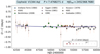 |
Fig. 1. Updated O − C diagram of V1344 Aql. The blue curve shows the best parabolic fit we obtained. The black error bars show the uncertainties as estimated by the Csörnyei et al. (2022) pipeline, while the red ones show the inflated errors according to the Hogg et al. (2010) definition. In the inset, the plotted point size refers to the corresponding uncertainty. |
The estimated period change rate is ∼10% higher than the Csörnyei et al. (2022) results, however, they are perfectly consistent within uncertainties. This estimate was used to infer the pulsation period at the chosen reference epoch in Eq. (1). According to the earlier analysis by Csörnyei et al. (2022), the pulsation period of V1344 Aql at the above reference epoch was estimated as P = 7.476713 ± 0.000004 days, compared to which the new value is 0.002% longer. The offset between the previous and new period estimates is due to the more advanced treatment of uncertainties and the scatter among the data through the Bayesian fitting. Owing to the high fitting uncertainties, as was pointed out by Szabados et al. (2014) as well, it is not possible to reliably separate the light-time effect caused by the orbital motion from the general scatter of the O − C points. This issue might be remedied by the future publication of the complete Harvard photometric plates archive (Grindlay et al. 2012), which will allow for the construction of a century-long O − C diagram along with a more precise view of the period changes.
3. New radial velocity data and orbit determination
Additionally to the data set presented in the discovery paper on spectroscopic binarity of V1344 Aql by Szabados et al. (2014), new RV data were collected using the 0.5 m RC telescope of ELTE Gothard Astrophysical Observatory, Szombathely and the 1 m RCC telescope of Piszkéstető Mountain Station of the Konkoly Observatory of the Research Centre for Astronomy and Earth Sciences. The spectra were taken with two different fibre-fed echelle spectrographs both installed on optical telescopes: the eShel system of the French Shelyak Instruments (Thizy 2011, R ≈ 11 000), used on both telescopes before 2014; and the spectrograph made by Astronomical Consultants & Equipment (ACE), with a resolution of R ⪅ 20 000 and mounted at the 1 m RCC telescope since 2014. The exposure times were between 600 s and 1200 s depending on weather conditions, seeing, and the telescope used. Th-Ar calibration spectra were taken before and after each observed target star in all cases. The data reduction was done using the same method as described in Szabados et al. (2014), that is, by applying standard tasks in IRAF2 including bias, dark and flat-field corrections, aperture extraction, wavelength calibration, and continuum normalisation. The consistency of the wavelength calibrations was checked using RV standard star observations, which proved the stability of the systems. The individual RV values were calculated using the cross-correlation technique with synthetic spectra from the Munari et al. (2005) library with resolution R = 11 500, and effective temperature Teff = 6000 K. We performed the calculations using the FXCOR task of IRAF in the wavelength range between 490 and 650 nm, excluding the wavelength range between 588 and 590 nm and 627 and 629 nm. Thus we did not include Balmer lines, NaD, and telluric regions in the cross-correlation. To calculate barycentric Julian dates and velocity corrections, the BARCOR code of Hrudková (2006) was used for the mid-exposure times of the observations.
The RV curves were calculated using the period and epoch given in Sect. 2. In order to achieve the best consistency, we refolded our previously published data (Szabados et al. 2014) to a phase curve using the new period. The folded phase curves are shown in Fig. 2, while the new RV values along with their uncertainties (calculated by fitting a parabola around the maximum value of the cross-correlation function) are listed in Table 1. We used the RV observations from 2012 to construct a template curve for determination of the γ velocity (velocity of the mass centre) of the Cepheid. We fitted a third-order Fourier-polynomial to the data, the γ velocities were then calculated for each observing season (year) and are presented in Table 2. Since we used the period determined for 2020, no phase shift was necessary to fit the template curves and calculate the γ velocities for each season. The template curves shown in Fig. 2 represent the γ-velocity variation of the system, which was done by shifting the curve vertically from 2012 with the appropriate γ velocities given in Table 2.
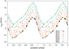 |
Fig. 2. Our RV data and the template curves for each year based on the fit to the data from 2012. The template curves are shifted vertically according to the γ velocities given in Table 2. |
New RV data for V1344 Aql.
γ velocities for V1344 Aql.
Our new RV data allowed us to determine the orbital solution for the system. The fitting process was performed in two steps: first the grid search method (Bevington & Robinson 2003) was applied using larger step sizes on a wider parameter space to find the location of the lowest χ2 values. This method limited the location of the global minimum of the fit. In the second step the gradient search method (Bevington & Robinson 2003) with χ2 minimisation was applied with varying step sizes to further restrict the orbital solution. The uncertainties of the fitted parameters were estimated using the bootstrap method (Efron & Tibshirani 1986) by calculating one thousand orbits with the gradient search method. Finally, the standard deviation of the one thousand solutions is given as the uncertainty for each parameter. Our orbital solution is given in Table 3 and shown in Fig. 3. We found that the orbital period of the system is approximately 34.6 yr with an orbital eccentricity of 0.22.
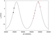 |
Fig. 3. Orbital solution with parameters given in Table 3. Our data are marked with red triangles, while black dots represent the earlier literature data (see Table 2). |
New orbital parameters for V1344 Aql.
4. Discussion and conclusions
Using our new RV data and updated pulsation period, we were able to determine the orbital solution for the binary Cepheid V1344 Aql. We constructed an updated O − C diagram based on the most recent observations to derive the recent pulsation period of the Cepheid.
Since the temporal coverage of the observations does not allow us to separate the tiny light-time effect from the scatter of the O − C values, we only used RV observations for the orbit determination. A larger number of RV observations per observing season gives a lower uncertainty in the γ velocities; however, a lower number of RV data covering the minimum and maximum phase are also useful for orbit determination. This can be seen in comparing our observations from 2020 and 2014: the four data points from 2020 include points close to the minimum and maximum velocity, and thus the γ-velocity has a much lower uncertainty compared to that of 2014, where the two data points do not cover these phases. The template curve fitting for 2014 still gives a γ velocity that can be used for the orbit determination, although resulting in a larger uncertainty.
The maximum orbital velocity is close to the γ velocity derived from our 2020 RV data, which has a huge impact on constraining the orbital solution. We examined the possibility of a period approximately half the length of the one given in Table 3, which could not be excluded without our latest data point. However, the χ2 value of this solution (including our latest point) was about 90 higher compared to the longer period orbit without matching the maximum velocity phase; thus, we excluded this solution as a possible fit. The orbital period of the system is approximately 34.6 yr with a relatively small eccentricity of 0.22. This confirms the finding of Szabados et al. (2014), suggesting a decades-long orbit for the system. RV and photometric observations in the forthcoming years will be crucial to disentangling and taking into account the light-time effect of the system and determining more accurate orbital elements.
Available at https://konkoly.hu/CEP/intro.html.
IRAF is distributed by the National Optical Astronomy Observatories, which are operated by the Association of Universities for Research in Astronomy, Inc., under cooperative agreement with the National Science Foundation.
Acknowledgments
The authors thank the referee for his/her constructive comments that helped to improve the quality of the paper. This project has been supported by the Lendület grant LP2012-31 of the Hungarian Academy of Sciences. A. Pál acknowledges support from the grant K-138962 of the Hungarian Research, Development and Innovation Office (NKFIH). L.K. acknowledges the support from the grants PD-134784, K-131508 and KKP-143986 of the Hungarian Research, Development and Innovation Office (NKFIH). L.K. is a Bolyai János Research Fellow. Financial support by the Hungarian National Research, Development and Innovation Office grant K129249 is acknowledged.
References
- Arellano Ferro, A. 1984, MNRAS, 209, 481 [CrossRef] [Google Scholar]
- Balona, L. A. 1981, Observatory, 101, 205 [NASA ADS] [Google Scholar]
- Berdnikov, L. N. 2008, VizieR Online Data Catalog: II/285 [Google Scholar]
- Bevington, P., & Robinson, D. 2003, Data Reduction and Error Analysis for the Physical Sciences (McGraw-Hill) [Google Scholar]
- Breuval, L., Kervella, P., Anderson, R. I., et al. 2020, A&A, 643, A115 [EDP Sciences] [Google Scholar]
- Csörnyei, G., Szabados, L., Molnár, L., et al. 2022, MNRAS, 511, 2125 [CrossRef] [Google Scholar]
- Derekas, A., Szabó, G. M., Berdnikov, L., et al. 2012, MNRAS, 425, 1312 [NASA ADS] [CrossRef] [Google Scholar]
- Efron, B., & Tibshirani, R. 1986, Stat. Sci., 1, 54 [Google Scholar]
- Eggen, O. J. 1985, AJ, 90, 1297 [NASA ADS] [CrossRef] [Google Scholar]
- Evans, N. R. 1992, ApJ, 389, 657 [CrossRef] [Google Scholar]
- Evans, N. E., Bond, H. E., Schaefer, G. H., et al. 2013, AJ, 146, 93 [NASA ADS] [CrossRef] [Google Scholar]
- Evans, N. R., Berdnikov, L., Lauer, J., et al. 2015, AJ, 150, 13 [NASA ADS] [CrossRef] [Google Scholar]
- Fernie, J. D., & Garrison, R. G. 1981, PASP, 93, 330 [NASA ADS] [CrossRef] [Google Scholar]
- Gaia Collaboration (Clementini, G., et al.) 2017, A&A, 605, A79 [NASA ADS] [CrossRef] [EDP Sciences] [Google Scholar]
- Grindlay, J., Tang, S., Los, E., & Servillat, M. 2012, in New Horizons in Time Domain Astronomy, eds. E. Griffin, R. Hanisch, & R. Seaman, IAU Symp., 285, 29 [NASA ADS] [Google Scholar]
- Hogg, D. W., Bovy, J., & Lang, D. 2010, ArXiv e-prints [arXiv:1008.4686] [Google Scholar]
- Hrudková, M. 2006, in WDS’06 Proceedings of Contributed Papers: Part III – Physics, eds. J. Safrankova, & J. Pavlu (Prague: Matfyzpress), 18 [Google Scholar]
- Karczmarek, P., Smolec, R., Hajdu, G., et al. 2022, ApJ, 930, 65 [NASA ADS] [CrossRef] [Google Scholar]
- Karczmarek, P., Hajdu, G., Pietrzyński, G., et al. 2023, ApJ, 950, 182 [NASA ADS] [CrossRef] [Google Scholar]
- Kervella, P., Gallenne, A., Remage Evans, N., et al. 2019, A&A, 623, A116 [NASA ADS] [CrossRef] [EDP Sciences] [Google Scholar]
- Kovacs, G., & Szabados, L. 1979, Inf. Bull. Var. Stars, 1719, 1 [NASA ADS] [Google Scholar]
- Moe, M., & Di Stefano, R. 2017, ApJS, 230, 15 [Google Scholar]
- Morokuma, T., Tominaga, N., Tanaka, M., et al. 2014, PASJ, 66, 114 [NASA ADS] [CrossRef] [Google Scholar]
- Munari, U., Sordo, R., Castelli, F., & Zwitter, T. 2005, A&A, 442, 1127 [NASA ADS] [CrossRef] [EDP Sciences] [Google Scholar]
- Neilson, H. R., Schneider, F. R. N., Izzard, R. G., Evans, N. R., & Langer, N. 2015, A&A, 574, A2 [NASA ADS] [CrossRef] [EDP Sciences] [Google Scholar]
- Pilecki, B., Thompson, I. B., Espinoza-Arancibia, F., et al. 2022, ApJ, 940, L48 [NASA ADS] [CrossRef] [Google Scholar]
- Pojmanski, G. 2001, in IAU Colloq. 183: Small Telescope Astronomy on Global Scales, eds. B. Paczynski, W. P. Chen, & C. Lemme, ASP Conf. Ser., 246, 53 [NASA ADS] [Google Scholar]
- Sterken, C. 2005, in The Light-Time Effect in Astrophysics: Causes and Cures of the O-C Diagram, ed. C. Sterken, ASP Conf. Ser., 335, 3 [NASA ADS] [Google Scholar]
- Szabados, L. 1991, Commun. Konkoly Obs. Hung., 96, 123 [NASA ADS] [Google Scholar]
- Szabados, L. 2003, Inf. Bull. Var. Stars, 5394, 1 [NASA ADS] [Google Scholar]
- Szabados, L., & Klagyivik, P. 2012, Ap&SS, 341, 99 [NASA ADS] [CrossRef] [Google Scholar]
- Szabados, L., & Nehéz, D. 2012, MNRAS, 426, 3148 [NASA ADS] [CrossRef] [Google Scholar]
- Szabados, L., Derekas, A., Kiss, L. L., et al. 2013, MNRAS, 430, 2018 [NASA ADS] [CrossRef] [Google Scholar]
- Szabados, L., Cseh, B., Kovács, J., et al. 2014, MNRAS, 442, 3155 [CrossRef] [Google Scholar]
- Thizy, O. 2011, in Active OB Stars: Structure, Evolution, Mass Loss, and Critical Limits, eds. C. Neiner, G. Wade, G. Meynet, & G. Peters, Proc. IAU, 272, 282 [NASA ADS] [Google Scholar]
- Winkler, C., Courvoisier, T. J. L., Di Cocco, G., et al. 2003, A&A, 411, L1 [NASA ADS] [CrossRef] [EDP Sciences] [Google Scholar]
Appendix A: O − C data
Table. A.1 shows the median V-band O − C values obtained for V1344 Aql. The underlying data are identical to those analysed in Csörnyei et al. (2022), except for the most recent KWS observations.
Obtained O − C values along with the source data references.
All Tables
All Figures
|
Fig. 1. Updated O − C diagram of V1344 Aql. The blue curve shows the best parabolic fit we obtained. The black error bars show the uncertainties as estimated by the Csörnyei et al. (2022) pipeline, while the red ones show the inflated errors according to the Hogg et al. (2010) definition. In the inset, the plotted point size refers to the corresponding uncertainty. |
| In the text | |
|
Fig. 2. Our RV data and the template curves for each year based on the fit to the data from 2012. The template curves are shifted vertically according to the γ velocities given in Table 2. |
| In the text | |
|
Fig. 3. Orbital solution with parameters given in Table 3. Our data are marked with red triangles, while black dots represent the earlier literature data (see Table 2). |
| In the text | |
Current usage metrics show cumulative count of Article Views (full-text article views including HTML views, PDF and ePub downloads, according to the available data) and Abstracts Views on Vision4Press platform.
Data correspond to usage on the plateform after 2015. The current usage metrics is available 48-96 hours after online publication and is updated daily on week days.
Initial download of the metrics may take a while.