| Issue |
A&A
Volume 684, April 2024
|
|
|---|---|---|
| Article Number | A119 | |
| Number of page(s) | 25 | |
| Section | Extragalactic astronomy | |
| DOI | https://doi.org/10.1051/0004-6361/202348659 | |
| Published online | 10 April 2024 | |
ALMA survey of a massive node of the Cosmic Web at z ∼ 3
I. Discovery of a large overdensity of CO emitters
1
Dipartimento di Fisica “G. Occhialini”, Università degli Studi di Milano-Bicocca, Piazza della Scienza 3, 20126 Milano, Italy
e-mail: This email address is being protected from spambots. You need JavaScript enabled to view it.
2
Institute of Theoretical Astrophysics, University of Oslo, PO Box 1029 Blindern, 0315 Oslo, Norway
3
INAF – Osservatorio di Astrofisica e Scienza dello Spazio, Via Gobetti 93/3, 40129 Bologna, Italy
4
Dipartimento di Astronomia e Scienza dello Spazio, Università degli Studi di Firenze, Largo E. Fermi 2, 50125 Firenze, Italy
5
INAF – Osservatorio Astronomico di Brera, Via Brera 28, 21021 Milano, Italy
6
INAF – Osservatorio Astronomico di Trieste, Via G. B. Tiepolo 11, 34143 Trieste, Italy
7
Kapteyn Astronomical Institute, University of Groningen, Landleven 12, 9747 AD Groningen, The Netherlands
8
Institute of Science and Technology Austria (IST Austria), Am Campus 1, 3400 Klosterneuburg, Austria
9
Department of Astronomy, University of Wisconsin-Madison, 475 N. Charter St., Madison, WI 53706, USA
Received:
17
November
2023
Accepted:
30
December
2023
Abstract
Submillimeter surveys toward overdense regions in the early Universe are essential for uncovering the obscured star formation and the cold gas content of assembling galaxies within massive dark matter halos. In this work, we present deep ALMA mosaic observations covering an area of ∼2′×2′ around MUSE Quasar Nebula 01 (MQN01), one of the largest and brightest Ly-α emitting nebulae discovered thus far; it surrounds a radio-quiet quasar at z ≃ 3.25. Our observations target the 1.2 and the 3 mm dust continuum as well as the carbon monoxide CO(4–3) transition in galaxies in the vicinity of the quasar. We identify a robust sample of 11 CO-line-emitting galaxies (including a closely separated quasar companion) that lie within ±4000 km s−1 of the quasar systemic redshift. A fraction of these objects were missed in previous deep rest-frame optical/UV surveys, which highlights the critical role of (sub)millimeter imaging. We also detect a total of 11 sources revealed in the dust continuum at 1.2 mm; six of them have either high-fidelity spectroscopic redshift information from rest-frame UV metal absorptions or the CO(4–3) line that places them in the same narrow redshift range. A comparison of the CO luminosity function and 1.2 mm number count density with those of the general fields points to a galaxy overdensity of δ > 10. We find evidence of a systematic flattening at the bright end of the CO luminosity function with respect to the trend measured in blank fields. Our findings reveal that galaxies in dense regions at z ∼ 3 are more massive and significantly richer in molecular gas than galaxies in fields, which enables a faster and accelerated assembly. This is the first in a series of studies aimed at characterizing one of the densest regions of the Universe found so far at z > 3.
Key words: galaxies: evolution / galaxies: high-redshift / galaxies: ISM / large-scale structure of Universe
© The Authors 2024
 Open Access article, published by EDP Sciences, under the terms of the Creative Commons Attribution License (https://creativecommons.org/licenses/by/4.0), which permits unrestricted use, distribution, and reproduction in any medium, provided the original work is properly cited.
This article is published in open access under the Subscribe to Open model. This email address is being protected from spambots. You need JavaScript enabled to view it. to support open access publication.
1. Introduction
The formation and evolution of galaxies and active galactic nuclei (AGN) is believed to occur within a network of diffuse intergalactic medium gas distributed along filaments and sheets on megaparsec-scale structures (the so-called Cosmic Web; Bond et al. 1996). Cosmological simulations predict that galaxy formation takes place in the densest regions of this structure, where the assembly of galaxies is regulated by the complex interplay between the accretion of gas from the Cosmic Web and gas ejection from galaxies into the intergalactic medium triggered by feedback mechanisms acting on galactic scales (such as star formation and AGN-driven outflows; see, e.g., McNamara & Nulsen 2012; Pike et al. 2014; Wilkinson et al. 2018). However, the details of these processes are still poorly understood. The collection of many lines of evidence over the years led to a growing consensus concerning the key role of the large-scale environment in shaping galaxies during their evolution, at least at z ≲ 1. Elliptical galaxies are preferably found in clusters (Oemler 1974; Davis & Geller 1976; Dressler 1980; Postman & Geller 1984; Dressler et al. 1997; Boselli & Gavazzi 2006) and tend to be passive (with red colors), while galaxies in fields are predominantly blue spirals that exhibit substantial star-formation activity (see, e.g., Lewis et al. 2002; Gómez et al. 2003; Balogh et al. 2004; Hogg et al. 2004; Kauffmann et al. 2004; Tanaka et al. 2004; Park et al. 2007; Peng et al. 2010). The situation at higher redshifts is, however, unclear. Some results suggest that the aforementioned trend holds up to z ∼ 2 (see, e.g., Postman et al. 2005; Muzzin et al. 2012; Quadri et al. 2012; Darvish et al. 2016; Fossati et al. 2017; Kawinwanichakij et al. 2017; Pérez-Martínez et al. 2023; Taylor et al. 2023), while others support the evidence of a higher star-formation activity in protoclusters at z > 2 compared to the field galaxies (e.g., Elbaz et al. 2007; Cooper et al. 2008; Ideue et al. 2009; Tran et al. 2010; Shimakawa et al. 2018; Ito et al. 2020, but see also Domínguez-Gómez et al. 2023), which is consistent with the hypothesis that galaxies in dense environments assemble their mass more rapidly and at earlier times (see, Alberts & Noble 2022 for a recent review and further discussion). In order to get further insights into how galaxies form and evolve in connection with their large-scale environment, it is therefore crucial to obtain a comprehensive view of overdense regions of galaxies at early epochs, especially during the peak of galaxy assembly and AGN activity at z ∼ 2 − 3 (Madau & Dickinson 2014).
At high redshifts, there is an increasing contribution from dusty star-forming galaxies to the cosmic star-formation rate density (see, e.g., Casey et al. 2014; Dunlop et al. 2017; Hodge & da Cunha 2020), meaning that a larger fraction of galaxies might remain undetected even in deep rest-frame optical/UV surveys, and possibly even in near-infrared (NIR) observations (e.g., Williams et al. 2019; Yamaguchi et al. 2019; Smail et al. 2021, 2023; Manning et al. 2022). Such galaxies can, however, be uncovered in the rest-frame far-infrared (FIR) band, where the thermal emission by dust grains dominates the galaxy spectral energy distribution. At such wavelengths, atomic fine-structure and molecular emission lines are the main coolants of the gas-phase galaxy interstellar medium, and they can therefore be targeted to trace the cold gas in galaxies (see Carilli & Walter 2013, for a review).
With the advent of sensitive facilities in the (sub)millimeter, such as the Atacama Large (sub)millimeter Array (ALMA), astronomers have started to map dense galaxy environments such as (proto-)clusters of galaxies at increasingly high redshifts to understand how cold gas – the ultimate fuel of star formation – and dust – which is a proxy of the galaxy metal enrichment – are affected in galaxy-rich environments with respect to galaxies living in isolation. Such studies have been mainly conducted by targeting carbon monoxide (CO) rotational lines, the singly ionized atomic carbon transition [CII]158 μm, or the FIR dust continuum at z ∼ 1 − 2 (e.g., Hayashi et al. 2017; Noble et al. 2017, 2019; Rudnick et al. 2017; Stach et al. 2017; Coogan et al. 2018; Williams et al. 2022), z ∼ 2 − 3 (e.g., Wang et al. 2016, 2018; Lee et al. 2017; Castignani et al. 2019; Gómez-Guijarro et al. 2019; Tadaki et al. 2019; Champagne et al. 2021; Jin et al. 2021; Aoyama et al. 2022), and up to z ∼ 3 − 4 (see, e.g., Hodge et al. 2013; Miller et al. 2018; Oteo et al. 2018; Umehata et al. 2019; Hill et al. 2020; Polletta et al. 2022). These investigations led to the discovery of numerous gas-rich galaxies in (the core of) galaxy (proto-)clusters. Nevertheless, despite all these efforts, the emerging picture is still unclear and contradictory, with tentative evidence of an enhanced star-formation rate, gas and dust fraction, and molecular gas excitation in clustered galaxies, at least at 1 < z < 2.
Crucially, the works cited above highlight the importance of submillimeter (pseudo-)blind surveys toward galaxy-dense regions at high z for probing galaxy CO luminosity functions (LFs) and the spectral-line energy distribution, as well as the millimeter number counts, which can provide us with key clues as to the physical processes that are acting in the nodes of the Cosmic Web. In this work, we present ALMA observations toward the MUSE Quasar Nebula 01 (MQN01) field. This field hosts a giant Ly-α-emitting nebula initially discovered via a blind survey of bright radio-quiet quasars (or quasi-stellar objects) at 3 < z < 4 (Borisova et al. 2016) using the Multi Unit Spectroscopic Explorer (MUSE) mounted on the Very Large Telescope (VLT). The MQN01 nebula surrounding the quasi-stellar object (QSO) CTS G18.013 at z = 3.25 is one of the largest nebulae (∼30″, corresponding to ∼230 physical kpc) discovered in this survey that also exhibits a filamentary morphology. The largest Ly-α nebulae discovered so far are often associated with an overdensity of AGN and massive (dusty) star-forming galaxies (see, e.g., Hennawi et al. 2015; Cai et al. 2017; Cantalupo 2017; Arrigoni Battaia et al. 2018a,b; Umehata et al. 2019; Nowotka et al. 2022). MUSE follow-up observations extending both the covered area and sensitivity limit mapped a large area, ∼4 arcmin2, around MQN01, revealing a high concentration of Lyman break galaxies (LBGs) embedded in an extended Ly-α-emitting structure (Cantalupo et al., in prep.; Galbiati et al., in prep.). To obtain a full picture of this exceptional field, we used ALMA to perform mosaic observations targeting the millimeter dust continuum and the CO(4–3) rotational transition in galaxies embedded in MQN01. This work is part of an extensive multiwavelength survey of the MQN01 field that has been conducted in the FIR to X-ray regime using multiple facilities. Here, we report galaxy detections and field statistics obtained via our millimeter observations using ALMA. The full characterization of individual sources and their correlation with the Ly-α-emitting gas will be presented in future works.
This paper is structured as follow: in Sect. 2 we present our survey design, the acquired observations, the reduction of the data, and the ancillary datasets. In Sect. 3 we discuss the source extraction and the measurements of the continuum fluxes and line luminosities of the selected candidates. In Sect. 4 we present our results, including the analysis of the CO LF and the millimeter-continuum source number count density. We dedicate Sect. 5 to the interpretation and discussion of our results and compare them with those of previous works, putting our findings into a more general context. Finally, in Sect. 6 we draw our conclusions.
Throughout this paper we assume a standard Λ cold dark matter cosmology with H0 = 67.7 km s−1 Mpc−1, Ωm = 0.310, and ΩΛ = 1 − Ωm from Planck Collaboration VI (2020).
2. Observations and data processing
2.1. Survey design
We observed the MQN01 field with ALMA 12-m array using band 3 and 6 in Cycle 8 (Program ID. 2021.1.00793.S, PI: S. Cantalupo). The observations were designed to cover the entire field of view (FoV) of the MUSE mosaic (∼4 arcmin2, corresponding to ≃16 cMpc2 at z = 3.25) by performing a Nyquist-sampled mosaics following the standard hexagonal pattern to achieve a uniform sensitivity across the entire field.
The band 3 mosaic consists of 27 pointings each with a half power beam width (HPBW) of ≃53″ resulting in a covered rectangular sky area of  . Observations were carried out in frequency division mode. The frequency setup consists of four 1.875 GHz-wide spectral windows (SPWs). We tuned two adjacent SPWs in the upper side band (USB) centered respectively at 107.20 GHz and 109.00 GHz such that they encompass the CO(4–3) transition (rest-frame frequency νrest = 461.041 GHz), as well as the underlying 3 mm dust continuum in a contiguous redshift bin of Δz ≃ 0.15 corresponding to Δv = ( − 4000, +6100) km s−1 around z = 3.25. We tuned the other two SPWs in the lower side band (LSB), covering a continuous bandwidth in the frequency range 94.06 − 97.74 GHz. The total effective bandwidth of ALMA band 3 observations is 7.354 GHz. The native spectral resolution of the acquired data is 1.95 MHz (∼5.4 km s−1). Observations were carried out in 18 execution blocks during the period 2022 January 16–May 19 employing a total on-source exposure time of 16.4 h and maximum antenna baseline of 976.6 m. During the executions, the quasars J0025-4803 and J2357-5311 were observed as phase and flux calibrator, respectively.
The band 6 mosaic consists of 114 pointing with HPWB ≃ 24″ covering a sky area of  . We employed a frequency setup in frequency division mode with two pairs of adjacent 1.875 GHz-wide SPWs that we disposed to cover the 1.2 mm dust continuum together with the CO(9–8) (νrest = 1036.912 GHz), as well as the adjacent transitions of the hydroxyl ion OH+(11–01) (νrest = 1033.119 GHz) that are redshifted in the ALMA band 6 at z ≃ 3.25. The two SPWs in the USB are centered respectively at 243.20 GHz and 245.00 GHz, sampling a contiguous CO(9–8) line redshift bin of Δz ≃ 0.06, corresponding to Δv = ( − 2400, +2100) km s−1 around z = 3.25. The SPWs in the LSB cover the frequency range 228.26 − 231.94 GHz. The effective total bandwidth is 7.35 GHz with a native frequency sampling of 3.9 MHz (∼4.8 km s−1). The observations were carried out in four execution blocks during the period 2022 April 3–13, for a total on-source observation time of 3.3 h and a maximum baseline of 500.2 m. For such observations, the quasars J0025-4803 and J2258-2758 were used as phase and flux calibrator, respectively.
In Table 1 we report the details of the observations presented in this work. In Fig. 1 we show the combined primary beam (PB) response of the mosaics in the two different bands together with the disposition of the pointings. The last execution block of band 6 observations was affected by increased noise during the last two scans, impacting the sensitivity of the mosaic pointings no. 77-114. As a result, the sensitivity in the northern part of the FoV is about 30% lower than in the mosaic center.
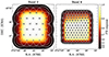 |
Fig. 1. Combined PB response for our ALMA mosaics at the representative frequency of 109.0 GHz (band 3, left panel) and for the aggregate continuum mosaic image of ALMA band 6 (right panel). The white contours correspond to a PB response of 30% (solid line) and 50% (dashed line). The circles show the disposition of the pointings with diameter equal to the HPBW of the ALMA 12 m antennas at the reference frequency of the setup. |
Characteristics of ALMA observations toward the MQN01 field.
2.2. Data reduction
We performed data reduction using the Common Astronomy Software Application (CASA; McMullin et al. 2007; Hunter et al. 2023). We calibrated the data of both band 3 and 6 observations by running the pipeline scripts (scriptForPI) delivered alongside with the raw measurement sets by using the CASA pipeline version 6.2.1. In the case of band 6 data, the calibration includes the re-normalization correction related to the ALMA amplitude normalization strategy. We imaged the ALMA band 3 and 6 visibilities by using the CASA task tclean by adopting a natural weighting scheme and by using “mosaic” as a gridding convolution function. We set the phase center at the coordinates ICRS 00:41:32.27 –49:36:19.60. In order to Nyquist sample the longest baselines we set pixel sizes of  and
and  for band 3 and 6 data, respectively. For each observation in ALMA band 3 and 6, we obtained two sets of “dirty” cubes (i.e., without performing the cleaning process) with a channel width of 25 km s−1 and 40 km s−1 in the LSB and USB, respectively. During the “cleaning” procedure, we set “cube” as spectral definition mode (specmode) and niter = 0. We also obtained dirty continuum images by aggregating all the four SPWs in each frequency setting and we performed the Fourier transform with the tclean by setting specmode = “mfs”. The resulting beam sizes of the ALMA band 3 data are
  and
and  for data cube at the reference frequency of 109.00 GHz and for continuum image, respectively. The data processing of ALMA band 6 observations yields beam sizes of
  and
and  for the continuum image and the data cube at the reference frequency of 245.00 GHz. After measuring the RMS (root-mean-square) of the dirty data and continuum images, we obtained “cleaned” data cubes and continuum images by setting tight circular apertures on ≥5σ sources in their continuum and we performed the cleaning using the tclean task down to 2σ (nsigma = 2).
2.3. Ancillary data
As part of our ALMA program, the presented mosaics have been complemented with an additional single high-resolution (∼0.25″) pointing encompassing the central region of MQN01 field using ALMA band 3. We designed these observations in order to spatially resolve the CO(4–3) line emission of the quasar host galaxy CTS G18.01, as well as those of possible closely separated galaxies. Full details and analysis of this data will be presented in a future paper. In the current work we use these data to disentangle the QSO line and continuum emission, which appear blended with a nearby companion located at ∼1″ sky-projected distance in the lower-resolution mosaics (see Sect. 3).
Our ALMA observations are part of an extensive multiwavelength observational campaign ranging from the (rest-frame) FIR to the X-ray regime using both ground-based and space telescopes. These data will be presented in full details in future works. In this study we benefit from some of the acquired data. Here we summarize the main characteristics of such observations.
In this work, we make use of deep VLT/MUSE spectroscopic observations toward the MQN01 field (Cantalupo et al., in prep.; Galbiati et al., in prep.). Such observations consist in four 10 h-pointing (40 h of total exposure time) using the MUSE wide field mode integral field spectrograph with adaptive optics covering a FoV of ≃2′×2′, which is fully sampled by our ALMA data. The MUSE observations provide us with integral field spectroscopy between 4650 − 9300 Å with a spectral resolution of R ∼ 2000 − 3500. In this field, galaxies are identified via their rest-frame far-UV (FUV) continuum emission in the white-light image. The final sample comprises only those sources with a high-confidence measurement of the spectroscopic redshift from interstellar absorption lines (e.g., SiII 1260,1526 Å, OI 1303 Å, CII 1334 Å, and CIV 1548,1550 Å). The catalog includes 38 galaxies with secure redshift between 2.7 < z < 4.3, 22 out of which lie within ±1000 km s−1 of the QSO CTS G18.01 systemic redshift (z = 3.25; Galbiati et al., in prep., for full details).
We imaged the MQN01 field in the optical by using the VLT Focal Reducer and low-dispersion Spectrograph (FORS2; Appenzeller & Rupprecht 1992) instrument by acquiring broadband mosaics (≃13 × 13 arcmin2) in U (central wavelength λ0 = 361 nm; ∼7 h of exposure time), B (λ0 = 440 nm; ∼5 h of exposure time) and R (λ0 = 655 nm; ∼45 min of exposure time) filters. Such observations cover a 36× larger sky area with respect to the MUSE mosaic. This allows us to extend the census of the z = 3.0 − 3.5 population of LBGs well beyond the MUSE FoV via color-color selection tested against the spectroscopic information available in the MUSE FoV (Galbiati et al., in prep.).
In this work, we additionally benefit from NIR photometric images taken with NIRCam (NIR Camera) instrument on board the James Webb Space Telescope (JWST; Rigby et al. 2023). Observations were acquired by using the extra-wide filters F150W2 and F322W2 in the short- and long-wavelength channel, respectively, with an on-source exposure time of 1632 s per filter. These images cover a total FoV of 2 × 5 arcmin2 across the two detectors of the camera, with one detector encompassing the sky area observed with MUSE.
3. Source search and characterization
We performed a blind search of continuum- and line-emitting sources in both our ALMA band 3 and 6 images and cubes by using the Python-based code LINESEEKER1 (see González-López et al. 2017a, 2019 for full details). This code was originally developed to search for line and continuum emission of galaxies in the ALMA Frontier Fields survey (see González-López et al. 2017a,b) and was subsequently employed in various other surveys such as the ALMA Spectroscopic Survey in the Hubble Ultra Deep Field (ASPECS; see, e.g., Decarli et al. 2019; González-López et al. 2019, 2020), the Multiwavelength Study of ELAN Environments (AMUSE2; see, e.g., Chen et al. 2021; Arrigoni Battaia et al. 2022), and the Northern Extended Millimeter Array (NOEMA) Molecular Line Scan of the Hubble Deep Field North (HDF-N; Boogaard et al. 2023). Here we summarize the operation and the main features of the code.
LINESEEKER adopts a matched-filter approach. The code combines adjacent spectral channels by convolving the data cube along the spectral axis using Gaussian kernels with a range of widths. The RMS of the resulting images is then estimated via a sigma clipping at 5σ to remove the spurious increases in the noise due to possibly bright lines or continuum emission within the convolved channels. Then all the voxels above a given signal-to-noise ratio2 (S/N) threshold are stored for each convolution kernels. Finally, a list of line (or continuum3) emitter candidates is generated by grouping voxels from the different channels corresponding to unique sources by using the Density-Based Spatial Clustering of Application with Noise (DBSCAN) algorithm (Ester et al. 1996) included in the Python package Scikit-learn (Pedregosa et al. 2011). The final S/N of the sources is then selected as the maximum value obtained through the different convolutions. DBSCAN is also able to recover extended sources traced by S/N ≥ 2 pixels; however, a visual inspection is needed in order to verify if the single extended source is actually composed by multiple blended sources along the line of sight.
For each source candidate selected by LINESEEKER, the code automatically estimates the probability of false-positive detection based on the source S/N. To this purpose, the code is run on the negative (i.e., multiplied by −1) cube or image. In a deep extragalactic field in the (sub)millimeter, the majority of the surveyed area is expected to be empty sky; hence, any “negative” peak is a realization of noise. The statistics of negative detections are then compared to those of the positive ones. The fidelity (or reliability) of a positive detection as a function of its S/N is therefore computed as
 (1)
(1)
where Nneg and Npos are the number of negative and positive detections at a given S/N, respectively. To compute the fidelity at any S/N following Eq. (1), LINESEEKER assumes that the noise in the data is Gaussian distributed and computes the best-fit model of the cumulative distribution of negative detections using a function of the form ![Mathematical equation: $ N[1-\mathrm{erf}({\mathit{S}/\mathit{N}}/\sqrt{2}\,\sigma)] $](/articles/aa/full_html/2024/04/aa48659-23/aa48659-23-eq16.gif) , where erf is the error function and N and σ are free parameters.
, where erf is the error function and N and σ are free parameters.
Other similar source-finding algorithms are available in the literature, such as FINDCLUMP (Walter et al. 2016) and MF3D (Pavesi et al. 2018), which mostly differ on details (such as the adopted spectral filter function). Comparisons between the codes yield consistent results to within ∼10% (see González-López et al. 2019).
3.1. 1.2 mm continuum-selected candidates
We performed a source search of 1.2 mm continuum-emitting galaxy candidates in MQN01 field by running LINESEEKER on the dirty continuum band 6 image, excluding the region with PB response < 50% in which the low telescope sensitivity enhances the fraction of spurious candidates. The dirty data are preferred over the cleaned ones since in the former the intrinsic properties of the noise are preserved. Also, we did not correct our dirty image for the PB response to preserve the spatial homogeneity of the noise across the FoV. We therefore extracted all S/N ≥ 3 detections, and we selected the source candidates with estimated fidelity of F ≥ 90% corresponding to S/N ≥ 4.7. With this method, we retrieved a total of nine sources, including the QSO CTS G18.01 and a closely (on-sky) separated source (hereafter, Object B) partially blended with the QSO.
We complemented our blind search of 1.2 mm continuum candidates in the field by cross-matching our MUSE catalog of high-z sources (z > 2.5; see Sect. 2.3) with the low-fidelity (F > 20%) sources selected by LINESEEKER. In this process, we cross-matched the on-sky spatial position of the MUSE and ALMA continuum sources within a separation limit of  . We chose this separation since it is about one half of the angular resolution of the ALMA image thus accounting for possible spatial offset between the ALMA low-S/N FIR- and MUSE FUV-continuum peak4. This separation also corresponds to the maximum observed angular distance between our ALMA candidates selected in the blind search and their MUSE counterparts. By doing so, we recovered two additional sources in the field. In Table 2 we report the final catalog of the eleven ALMA 1.2 mm continuum-selected sources. In Fig. 2 we show the location of the sources detected by MUSE within ±1000 km s−1 of QSO CTS G18.01 and the ALMA 1.2 mm continuum-selected sources in the MQN01 field. We label the ALMA continuum sources C01–C09.
ALMA 1.2 mm continuum-selected sources.
 |
Fig. 2. Footprints of our ALMA and MUSE observations toward the MQN01 field. The orange and blue contours encircle the area where the combined mosaic PB response is ≥0.5 for ALMA band 3 and 6, respectively. Within these areas we performed the source search. Violet contour draws the MUSE footprint. The background is a composition of the JWST NIRCam F322W2 image (center and southeast corner) complemented with the VLT/FORS2 R-band observation (northeast, northwest, and southwest corners, and the southeast gap between the JWST NIRCam detectors). The point-spread-function-like emission of QSO CTS G18.01 has been subtracted in the JWST image revealing a nearby southeast quasar companion (Object B). Orange circles and blue squares indicate the locations of the ALMA CO(4–3) line-emitting and 1.2 mm continuum-selected sources in our ALMA band 3 and 6 observations, respectively. Green squares pin-point galaxy candidates detected in continuum at 3 mm in ALMA band 3. Gray hexagons denote sources corresponding to low-z counterparts, all but i5 show bright emission line in ALMA band 3. Violet crosses are the MUSE-selected LBGs belonging within ±1000 km s−1 of the QSO CTS G18.01 systemic redshift. The dashed red circle shows the inner 100 pkpc around the estimated center of the protocluster core. |
3.2. CO(4–3) line-emitting candidates
We used LINESEEKER to blindly search for CO(4–3) emission lines that are expected to be redshifted in the USB of the ALMA band 3 datacube. We opted to extract sources in the dirty cube not corrected for the PB response over the area where the combined mosaic sensitivity is ≥50% (see also, Sect. 3.1). We run the line-search algorithm on the datacube that we spectrally binned at 25 km s−1 using Gaussian kernels with widths ranging from 0 to 18 channels. This range enables the code to match the typical linewidths of CO lines observed in high-z galaxies (FWHM ∼ 50 − 1000 km s−1; see, e.g., Carilli & Walter 2013). We extracted all line-emitting candidates with estimated S/N ≥ 3. We then selected those sources with estimated fidelity of F ≥ 90% (see Sect. 3). Similarly to the search of 1.2 mm continuum emitters, we cross-matched the location of the MUSE LBGs with the low-fidelity (F > 20%) line-emitting candidates from LINESEEKER within a separation limit of  . As a result of this procedure, we extracted one additional source. The CO-based redshift of this candidate is within ±200 km s−1 with that based on the Ly-α emission line derived from MUSE spectroscopic data. The difference is consistent with the typical shift observed between the Ly-α line and the systemic redshift of high-z Ly-α emitters (see, e.g., Guaita et al. 2013; Muzahid et al. 2020a,b, 2021). Within the selected sample of 13 galaxies, we identified two interlopers at lower redshifts (dubbed “i3” and “i4”), which we therefore excluded from the final sample (see Sect. 3.5, for a detailed discussion). In Table 3 we report the final catalog of the eleven ALMA CO(4–3) line-emitting candidates. In Fig. 2, we draw the location of these galaxies (L01–L09) as well as those of the identified low-z interlopers within the field.
ALMA CO(4–3) line-selected sources.
3.3. 3 mm continuum-selected candidates
Similarly to what described in Sect. 3.1, we complemented our source extraction by searching candidates detected in continuum at 3 mm. For this purpose, we run LINESEEKER on the dirty aggregate (LSB+USB) continuum ALMA band 3 image. This blind search resulted in six continuum-detected sources (including the QSO and Object B) with fidelity F ≥ 90%. We also carefully inspected the ALMA 3, mm-continuum image in the position of secure sources (F = 100%) revealed in the ALMA band 6 at 1.2 mm. We therefore included two additional sources in the final sample corresponding to C04 and C05 (see Table 2), which show convincing continuum emission at 3 mm. We verified our conclusion by cross-matching the catalog of secure positive continuum detections at 1.2 mm with that at 3 mm provided by LINESEEKER. Finally, the cross-match between the catalog of high-z MUSE LBGs and 3 mm-continuum candidates did not provide us with any additional source. The locations of these detections in the MQN01 field are indicated in Fig. 2 by green squares.
3.4. Completeness and flux boosting
In order to compute the source number counts and the CO(4–3) LF, it is crucial to determine the probability of detecting sources in our blind search. Such information is enclosed in the continuum and CO line completeness functions. In addition, we need to estimate how the measured fluxes are affected by the noise in the real data. Indeed, sources with low S/N have a higher probability of being recovered with higher fluxes than the intrinsic value because of the boosting effect produced by the noise fluctuations (the so-called flux-boosting effect; see, e.g., Hogg & Turner 1998; Scott et al. 2002; Coppin et al. 2006). We computed the completeness of our survey by following a common approach widely adopted in the literature (see, e.g., Hatsukade et al. 2016, 2018; Umehata et al. 2017; González-López et al. 2019, 2020; Béthermin et al. 2020; Boogaard et al. 2023). We injected artificial sources in the real data and we then performed the source search by using LINESEEKER. More details about this exercise and how it is used to perform the corrections to the LFs are described in the following.
To estimate the completeness function of 1.2 mm-continuum detections in the ALMA band 6 we created artificial point-like sources by rescaling the synthesized beam model and we injected them into the dirty ALMA Band 6 continuum map at random positions within the source-search area of our survey (i.e., where the combined mosaic PB response is ≥50%). To take into account the effect of the variation of sensitivity across the mosaic field, we rescaled the source fluxes by the PB response at the input location of each source. We then run the source-search algorithm and we computed the source detection rate. We considered a source recovered if it is extracted within 1″ from its input location with a fidelity ≥90%. We repeated this procedure by injecting 20 sources simultaneously in the image and iterating for 100 times for each 1.2 mm flux density value within the range 0.02 − 0.46 mJy in steps of 0.02 mJy. The total number of injected sources in the simulation is 46 000. During the simulation we also evaluated the effect of flux boosting by computing the ratio of measured-to-injected flux of the artificial sources as  . In Fig. 3 we report the output of our simulation. As a result, the completeness in the flux range of the detected sources is in the range 50 − 100%, while the flux boosting effect does not affect significantly the measured 1.2 mm flux density of our selected sample of galaxies.
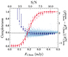 |
Fig. 3. Completeness (red squares, left axis) and flux boosting (blue circles and density plot, right axis) corrected for the PB response as a function of 1.2 mm flux density (bottom axis) and S/N (top axis) of injected sources in the ALMA band 6 continuum image. The error bars are derived by computing the 16th and 84th percentile of the distributions of completeness and flux boosting measurements in each flux bin. The solid red line is the best-fitting function to the completeness values modeled as C(F1.2 mm) = {1 + erf[(F1.2 mm − A)/B]}/2 with A = 0.197 ± 0.004 and B = 0.083 ± 0.007. The density plot shows the values of the flux boosting as a function of the measured flux of the injected sources. |
We evaluated the completeness of our blind survey of line-emitting sources and the effect of the flux boosting on the observed line emission. On the basis of the line measurements of the selected CO(4–3) emitters, we injected point-like artificial emission lines using a Gaussian spectral profile with a full width at half maximum (FWHM) and a velocity-integrated flux ranging within 100 − 1000 km s−1 in steps of 100 km s−1 and 0.02 − 0.5 Jy km s−1 in steps of 0.02 Jy km s−1, respectively. We injected the artificial sources at random positions (within the volume where the mosaic PB response is ≥50%) in the USB of the dirty ALMA band 3 cube binned at 25 km s−1 (i.e., where we search for the CO(4–3)-line emitting candidates; see Sect.3.2). We then rescaled the signal from the artificial line emitters in each channel of the cube by the PB response at the input position of the sources. We then ran LINESEEKER and we computed the source detection rate following the same criteria adopted for the artificial sources in the continuum. To estimate the line flux boosting effect for the recovered sources, we obtained the line-velocity integrated map using channels within ±2σ of the line centroid provided by LINESEEKER5. We then measured the total source fluxes by performing fit of the moment-0 map by using a two-dimensional Gaussian model6. For each values of the line FWHM and line-velocity integrated flux, we injected simultaneously 50 sources in the cube for a total of 12 500 sources injected in the whole simulation. In Fig. 4 we report the output of our simulation. As a result the selected sample is complete for line fluxes ≳0.4 Jy km s−1 while the flux boosting effect has negligible impact on the line measurements of our selected sample of CO(4–3) line-emitting galaxies.
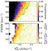 |
Fig. 4. Completeness (top panel) and flux boosting (bottom panel) corrected for the PB response as a function of the line-velocity integrated flux and the line FWHM of the injected sources in the ALMA band 3 dirty cube binned at 25 km s−1. In the top panel, the green line indicates where the completeness is ≥90%. |
3.5. Identification of interlopers across the redshift range
For the purpose of our analysis it is crucial to identify possible interlopers at different redshifts among the ALMA-selected galaxies. In the ALMA 3 mm band, sources at any redshift are expected to be revealed by their line emission, primarily via CO rotational lines, or the fine-structure transitions of the atomic neutral carbon [CI]609, 370 μm (though the latter are expected to be much fainter than low-J CO lines; see, e.g., González-López et al. 2019; Decarli et al. 2020 but see also Gullberg et al. 2016). In Fig. 5, we draw the redshifted frequency of such transitions entering our ALMA band 3 SPWs up to z = 6. The various transitions probe galaxies within different redshift intervals and cosmological volumes depending on the surveyed sky area and the encompassed frequency range (see Table 4). By using the available best-fit model to the CO LFs from Boogaard et al. (2023), we computed the number of expected galaxies at various redshifts within the cosmological volume probed by our observations above the limiting luminosity (see Table 4). As a result, ∼2 sources at z ∼ 1.1 are expected to be detected via their CO(2–1) line in the USB of our ALMA band 3 survey, ∼1 at z ∼ 2.2 through CO(3–2) line, and ∼0.5 CO(5–4) line emitters at z ∼ 4.3. For the targeted CO(4–3) line the number of expected sources is ∼2.5, dropping to ∼0.5 when considering the volume within ±1000 km s−1 around the QSO CTS G18.01. However, these estimates suffer from large uncertainties given the poor sampling of the CO LFs (see, e.g., Decarli et al. 2019, 2020; Boogaard et al. 2023) and therefore must be taken with caution.
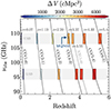 |
Fig. 5. Observed frequency of CO and [CI]609 μm transitions as a function of redshift. The boxes encircle both the frequency and redshift ranges covered by our ALMA band 3 observations. Boxes are color-coded by the cosmological volume probed by each transitions. Gray bands show the SPW coverage in the LSB and USB. The mean redshift of transitions entering the USB are also reported. The blue arrow points to the box representing the volume within ±1000 km s−1 around the QSO CTS G18.01 systemic redshift. |
Redshift bin, cosmological volume, and limiting luminosity of the main emission lines entering the USB of our ALMA band 3 survey.
In order to unambiguously identify the emission lines observed in our survey, we made use of our multiwavelength datasets of the MQN01 field. As described in Sect. 3.2, our blind search for CO(4–3) line-emitting candidates yielded an initial sample of 13 sources. Within the candidates belonging to this sample, 4 of out 13 (≃30%; L03, L07, L08, i4, excluding Object B) do not correspond to any high-z MUSE-selected LBGs/AGN. In addition, three candidates (L05, L06, i3) are located outside the MUSE mosaic footprint. For the first group of galaxies, the analysis of their MUSE spectra enabled us to identify i4 as a low-z interloper. The spectrum of this galaxy shows MgII] 2796,2803 Å absorptions and [OII] 3726,3729 Å line emission, the wavelengths of which unambiguously place this object at z ≃ 1.170; hence, the observed line emission in our ALMA band 3 observation is the CO(2–1) at the redshifted frequency of 106.2 GHz. In the case of sources outside the area surveyed by MUSE, the analysis of UBR colors obtained from VLT/FORS2 observations (see Sect. 2.3; Galbiati et al., in prep., for full details) allowed us to identify, at high confidence, i3 as another one low-z galaxy interloper. The line emission of i3 in our ALMA band 3 is observed at 109.2 GHz, the frequency of which possibly corresponds to either the CO(2–1) at z ≃ 1.11 or CO(1–0) z ≃ 0.06. Future spectroscopic follow-up observations will possibly pin down the precise redshift of i3. As a result of these analysis, we excluded the aforementioned two sources from the final sample of CO(4–3) line-emitting candidates.
In order to identify other possible additional interlopers belonging to our samples, we inspected band 3 and 6 datacubes at the locations of the CO(4–3), 1.2, and 3 mm selected candidates to look for the presence of any other emission lines. Doing so, we identified two galaxies: one, dubbed “i1”, that belongs to the sample of the 1.2 mm continuum-selected candidates (C06), and one, “i2”, that is detected in its continuum emission at 3 mm. Both show a very bright emission line in the LSB of the ALMA band 3 datacube. Via the analysis of the MUSE spectra, we accurately determined the redshift of i2 to be z ≃ 1.42, therefore identifying the detected line as the CO(2–1). Regarding i1, its redshift determination is highly uncertain given the lack of clear absorption or emission features in the MUSE datacube. However, the carefully inspection of the rest-frame UV spectrum of i1 points to a tentative redshift measurement of z ≃ 2.54, thus suggesting that the emission line we detected in our ALMA observations corresponds to the CO(3–2) transition.
We then assessed the nature of our ALMA continuum selected sources at 1.2 mm by inspecting their MUSE spectra. Among these, 6 out of 11 (QSO, C01, C02, C06, C08, and C09) have high-confidence spectroscopic redshifts derived from their rest-frame UV spectra, while the remaining 5 (C03, C04, C05, and C07) are either not detected in MUSE or the available spectrum does not allow us to determine a precise spectroscopic redshift. For the first group, the spectroscopic information available places four of them in the proximity of the QSO CTS G18.01 redshift; three of them (QSO, C01, and C02) have CO(4–3) detection, and the fourth (C08) is only detected in its dust continuum at 1.2 mm. The other two sources for which redshift measurements from MUSE are available are C06 and C09. C06 is the 1.2 mm continuum counterpart of the interloper i1, possibly detected via the CO(3–2) in the LSB of our ALMA band 3 observations. The MUSE spectra of C09, instead, exhibits SiIV 1394,1403 Å and CIV 1548,1550 Å absorption lines thus determining that this source is an interloper located at z ≃ 2.874. At this redshift, we do not expect to detect any bright emission line in our ALMA datacubes. We dubbed this source “i5”.
In summary, among all the sources extracted with high fidelity from our ALMA data, we unambiguously identified five interlopers located to different redshifts with respect to the QSO, namely i1 (z ≃ 2.54), i2 (z ≃ 1.42), i3 (either z ≃ 1.11 or z ≃ 0.06), i4 (z ≃ 1.170), and i5 (z ≃ 2.874). Interestingly, these findings are consistent to our predictions based on the CO LFs of blank fields.
However, the subsample of secure sources with two independent redshift measurements from both MUSE and the CO(4–3) line is composed by QSO, L01 (C01), L02 (C02), L04, and L09, all lying within ±1000 km s−1 of the QSO systemic redshift. Regarding the remaining sources, both Object B and L03 (C04) are either revealed in the millimeter dust continuum with ALMA or have a counterpart in the optical/NIR (see Appendix A). The analysis of VLT/FORS2 UBR colors of L03 (C04) suggests that this source belong to z ∼ 3 − 3.5 thus supporting the conclusion that L03 is actually detected via CO(4–3) at z ≃ 3.25. Finally, the recently acquired spectrum of Object B with the NIR spectrograph on board JWST definitely confirms that this source is located in the proximity of the QSO (Pensabene et al., in prep.). On the other hand, L05, L06, L07, and L08 are only detected in line with ALMA. Therefore, we cannot rule out that the latter sources actually represent either false-positive detections or interlopers located at different redshift. Future deep NIR observations are needed to assess the nature of such objects. Interestingly, these sources exhibits a large velocity shift and significant spatial separation from the QSO. In what follows, we took the aforementioned considerations into account in the computation of the CO LF.
3.6. Source fluxes and luminosities
The majority of CO(4–3) and continuum emitters detected in this work appear as compact spatially-unresolved sources. For such objects, the total continuum or line flux can be measured through a standard single-pixel analysis of the data. However, in the case of partially resolved objects or extended sources with complex morphology, this simple method results in significant flux underestimation. In this work, for such sources we therefore performed source flux measurements by applying the 2σ-clipped photometry7 (see, e.g., Béthermin et al. 2020) as described below.
We measured the 1.2 and 3 mm flux of the sources from the cleaned ALMA band 6 and 3 continuum images, respectively, not corrected for the combined mosaic PB response. For each source, we sum the flux density in mJy beam−1 enclosed in the contiguous area around the source including all pixels with S/N ≥ 28. We then divided the total flux density per beam by the synthesized beam area (in pixel units) and we rescaled the flux for the PB response at the location of the source. We computed the flux uncertainty by rescaling the noise by the square root of the number of independent beams within the integration area. In Table 2 we report our source flux measurements as well as their peak flux in the continuum. To understand which sources can be considered point-like, we computed the uncertainty-normalized difference between the two flux estimates as  , where F2σ, Fpeak, σ2σ, and σpeak are the 1.2 mm continuum flux obtained via the 2σ-clipped photometry, the peak flux, and their uncertainties, respectively. Within this formalism, we expect sources that are significantly resolved to have ΔF > 1. Sources C01 and C02 are such cases; for them we therefore adopted
  as our fiducial 1.2 mm continuum flux density measurement9. We however note that a proper flux measurement of QSO CTS G18.01 and its closely separated companion (Object B) is challenging due to the partial blending of the sources at the current resolution of the continuum data (see Sect. 2.2). In order to minimize the flux contamination, for such sources we adopted their 1.2 mm continuum flux peak
  .
.
We measured the CO line fluxes by following the iterative process presented in Béthermin et al. (2020). As for the continuum, the CO line emission of the QSO CTS G18.01 and Object B are partially blended. To measure their fluxes in what follows, we employed the ALMA band 3 high-resolution (∼0.25″) data (see Sect. 2.3) where the line emission of the sources are spatially resolved. For each CO(4–3)-line emitter we extracted the spectrum at the peak position of the source from the cleaned ALMA band 3 datacube binned at 40 km s−1. We then scaled the source spectrum by the PB response, and we performed a fit using a Gaussian profile for the line and a constant for the underlying 3 mm dust continuum using the curve_fit task included in the SciPy package (Virtanen et al. 2020). We then produced the line-velocity integrated map using all the channels within ±2σ from the line centroid. Subsequently, we re-extracted the source spectrum by summing all the spectra in pixels showing S/N ≥ 2 in the moment-0 map, and we rescaled the channel fluxes and their uncertainties respectively by the synthesized beam area, and the square root of the number of independent beams within the integration area. In this process, we masked all the pixels below the chosen threshold, which we confidently believe to be not related to any real emission from the source. This new spectrum is more informative in the case of (partially) resolved sources since it includes the signal from the entire source line-emitting region. We therefore performed a new spectral fit using the best-fit parameters of the previous iteration as starting point for the fitting code. We repeated the aforementioned steps a few times until convergence. All the extracted source spectra remain stable after a few iterations (< 10). Similarly to continuum flux estimates discussed above, we computed the quantity ΔF for each source. As a result, L01, L02, the QSO, and Object B10 all exhibit ΔF > 1. Accordingly, this analysis determined our final source spectra. We finally performed a finer fit of the final source spectrum by sampling the parameter space through the Python Markov chain Monte Carlo (MCMC) ensemble sampler emcee (Foreman-Mackey et al. 2013). We employed flat priors on the basis of the best-fit parameters derived from the last iteration and we assume Gaussian uncertainties in the definition of the likelihood. We finally derived the line luminosities as (see, e.g., Solomon et al. 1997)
![Mathematical equation: $$ \begin{aligned} L_{\rm CO}\left[L_{\odot }\right]&=1.04\times 10^{-3}S\Delta v\,\nu _{\rm obs}\,D_{L}^{2},\end{aligned} $$](/articles/aa/full_html/2024/04/aa48659-23/aa48659-23-eq104.gif) (2)
(2)
![Mathematical equation: $$ \begin{aligned} L{\prime }_{\rm CO}\left[{\mathrm{K\,km\,s}^{-1}\,\mathrm{pc}^{2}}\right]&=3.25\times 10^{7}S\Delta v\frac{D_{L}^{2}}{\left(1+z\right)^{3}\nu _{\mathrm{obs}}^{2}}, \end{aligned} $$](/articles/aa/full_html/2024/04/aa48659-23/aa48659-23-eq105.gif) (3)
(3)
where SΔv is the velocity-integrated line flux in Jy km s−1, νobs is the observed central frequency of the line in GHz, z is the source redshift measured from the CO line centroid, and DL is the luminosity distance in Mpc. The relation between Eqs. (2) and (3) is  , where νrest is the line rest frequency in GHz.
As our observations probe the (rest-frame) FIR wavelengths of high-z galaxies, the cosmic microwave background (CMB) might have an impact on our continuum and line measurements by increasing both the dust and the line excitation temperature. In addition, the CMB provides a strong background signal (see da Cunha et al. 2013; Zhang et al. 2016).
By assuming a modified black body with typical values for submillimeter galaxies (SMGs) at z ∼ 3 (i.e., spectral index 1.6 and dust temperature of 35 K; see, e.g., Kovács et al. 2006), the CMB affects our 1.2 mm dust continuum measurements by ≲5% and is thus compatible with the typical uncertainties on our flux estimates. The CMB effect further decreases assuming higher dust temperature.
Regarding the CO(4–3) line measurements, under the assumption of local thermodynamic equilibrium (i.e., the line excitation temperature equaling the gas kinetic temperature), the effect of CMB in reducing the recovered line fluxes is always < 20% for any excitation temperature > 40 K at z ≲ 4 (see Decarli et al. 2020). However, due to the unknown excitation temperature of the gas and the unverified assumption of local thermodynamic equilibrium for our sources, in this work we opted to not apply the CMB-related corrections (see, e.g., Decarli et al. 2020; Boogaard et al. 2023).
We list the measured fluxes and derived quantities of the lines in Table 3, and we report the final source spectra in Fig. 6. In Fig. 7 we report the source maps of the combined sample sources within |ΔvQSO|< 4000 km s−1 either detected in their CO(4–3) line or continuum at 1.2 mm.
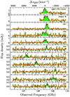 |
Fig. 6. Spectra of the CO(4–3) line-emitting sources in our ALMA survey of the MQN01 field. The red lines are the best-fit models to the spectra (yellow bins). The green bins indicate the channels we used to compute the line-velocity integrated maps (see Fig. 7) defined within ±2σ of the best-fitting Gaussian line. The horizontal gray bands are the rms noise in each channel. The blue vertical line indicate the QSO CTS G18.01 systemic velocity. Sources are labeled according to the IDCO reported in Table 3. |
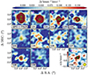 |
Fig. 7. Maps of the ALMA-selected galaxies in the MQN01 field detected in their CO(4–3) line, in the continuum at 1.2 mm, or in both. The color scale at the top refers to line-velocity integrated maps for all sources except C08, which is only detected at 1.2 mm in the dust continuum (bottom right color scale). Solid gray and black contours correspond to the velocity-integrated and 1.2 mm dust continuum maps, respectively and scales as [2, 3, 2N]×σ with N > 1 integer number. Dotted contours are the −2σ level. The yellow ellipse drawn in the bottom right corner represents the FWHM of the synthesized beam of the ALMA band 3 (yellow fill and gray line) and 6 (black line) observations. Sources are labeled according to the IDCO and/or ID1.2 mm reported in Table 3. Sources with spectroscopic-redshift confirmation are marked with a violet square in the upper-left corner. |
4. Results
4.1. CO luminosity function analysis
We computed the CO(4–3) LF by following the approach described in Decarli et al. (2016, 2019, 2020), Riechers et al. (2019), Boogaard et al. (2023). We define the CO LF as
![Mathematical equation: $$ \begin{aligned} \Phi _{\rm CO}\,\!\left( \mathrm{log}\,L{\prime }_{\rm CO} \right) \left[ \mathrm {cMpc}^{-3}\,dex^{-1} \right] = \frac{1}{\Delta V\,\Delta \,\mathrm{log}\,L{\prime }_{\rm CO}}\sum _{i}\frac{F_{i}}{C_{i}}, \end{aligned} $$](/articles/aa/full_html/2024/04/aa48659-23/aa48659-23-eq107.gif) (4)
(4)
where Φ is the number of sources per comoving Mpc3 in the luminosity interval  , ΔV is the comoving volume of our survey, and Fi and Ci are the fidelity and completeness associated with each source, respectively. We computed two different CO LFs, one in ΔV corresponding to the redshift range within ±4000 km s−1 of the systemic redshift of QSO CTS G18.01 (ΔvQSO) and one within |ΔvQSO|< 1000 km s−1. The corresponding cosmological volumes are respectively ΔV4000 = 2395 cMpc3 and ΔV1000 = 599 cMpc3. While ΔV4000 contains all our eleven CO(4–3) line-emitting candidates, ΔV1000 encompasses only sources having a optical/NIR counterparts (see also Appendix A) with a spectroscopic-confirmed redshift, thus including secure sources (F = 1). In this regard, we use sources in ΔV1000 to obtain a “raw” CO LF without applying the completeness correction.
To obtain the CO LF in the MQN01 field, we performed a Monte Carlo simulation of 1000 independent realizations of the LF. In each iteration, we varied the CO line luminosity, line FWHM, and the source fidelity of our CO line emitters within their uncertainties. For secure sources, we fixed the fidelity value to F = 1, for all the other sources we treated the fidelity as upper limit. This approach provides a conservative treatment of our fidelity estimates attempting to include the systematic uncertainties associated with sources without any clear multiwavelength counterparts (see, e.g., Pavesi et al. 2018; Decarli et al. 2019; Riechers et al. 2019). In each iteration, we extracted a number (P) from a random uniform distribution in the interval [0; 1]. We then selected the sources entering the realization that have P ≤ F. In this way, sources with higher fidelity have a larger chance to be selected. We computed the number of sources and associated 1σ Poisson confidence intervals (Gehrels 1986) in 0.5 dex bins. We then rescaled the resulting counts and uncertainties by the completeness corrections11, and then divided them by the effective volume of the survey and by the luminosity bin width. Finally, we averaged over the realizations. We repeated the entire simulation five times by shifting the luminosity bins of 0.1 dex in order to mitigate the dependence of the result on the bin definitions and to expose the intra-bin variations. For bins with a less than one count on average, we report a 1σ upper limit. The resulting CO(4–3) LF is shown in Fig. 8a (red and gold symbols; see the caption for a detailed explanation). In the same figure, we also show the LF derived from blank fields at the same redshift reported from the literature.
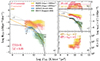 |
Fig. 8. Overdensity of CO emitters in the MQN01 field. Panel a: CO(4–3) LF in MQN01 and in blank fields. The (dark/light) red dots and boxes represent the CO LF in MQN01 field (fidelity (F) + completeness (C)-corrected/uncorrected, respectively) in ΔV4000, while gold hatched boxes are the uncorrected (raw) CO LF within ΔV1000. The blue and green boxes with black dots are data from ASPECS and HDF-N, respectively, which are representative of blank fields at these redshifts (e.g., Decarli et al. 2019, 2020; Boogaard et al. 2023). The downward arrows indicate 1σ upper limits. The dashed black line is the best-fit Schechter function to the ASPECS+HDF-N data reported in Boogaard et al. (2023). The orange line is the CO(4–3) LF prediction from SIDES simulation (Béthermin et al. 2022; Gkogkou et al. 2023) at z = 3 − 3.25. Gray lines represent the rescaled versions of such models. Panel b: Number of sources in each luminosity bin averaged over the iterations. The horizontal dashed line reports the total average number of sources entering each bin of the LFs. Panel c: Cumulative source number density as a function of the CO(4–3) line luminosity obtained by integrating the CO LFs. Panel d: Source overdensity in MQN01 field as a function of the CO(4–3) line luminosity obtained by a bin-to-bin ratio of the cumulative source number densities. |
Our aim is to compare the CO LF in MQN01 with those of blank fields. To do so, we combined data from ASPECS Walter et al. (2016), González-López et al. (2019), Decarli et al. (2019, 2020) and Boogaard et al. (2023), who performed a blind search of molecular lines in the HDF-N using NOEMA. These works provide us with the most up-to-date CO(4–3) LF at z ≃ 3.5. To enable a direct comparison with our result in the MQN01 field, we recomputed LFs consistently as described above adopting common luminosity bins. Additionally, we obtained the CO(4–3) LF from the Simulated Infrared Dusty Extragalactic Sky (SIDES) simulation (Béthermin et al. 2022; Gkogkou et al. 2023) at z = 3 − 3.5. As a comparison, in Fig. 8 we also rescaled the best-fit Schechter function to the blank fields by a factor of 8 (see Boogaard et al. 2023) as well as the CO LF predicted from SIDES. Interestingly, the CO LF in MQN01 differs significantly not only in normalization but also in shape with respect to those of blank fields showing a flattening at its bright end. We further discuss this point in Sect. 5.
We then computed the cumulative source number counts per comoving volume nCO(>  ) by integrating the five different CO LFs separately, each of which has uncorrelated luminosity bins. We show our results in Fig. 8c. We also obtained cumulative source number counts from both the best fit of blank fields and SIDES by integrating the corresponding CO LFs. In Fig. 8 we also rescaled the blank field cumulative functions by a factor of 25 to compare them to our results.
Finally, we evaluated the galaxy overdensity δ(>  ) as traced by CO(4–3) by computing the bin-to-bin ratios between the cumulative number counts in MQN01 and those in blank fields. The measured cumulative overdensity of CO(4–3) line emitters is a strong function of luminosity, increasing from ∼8 (at the lowest luminosities) to ∼200 (at the highest luminosities). Above the limiting CO luminosity of our survey we estimated
  and
and  , in ΔV4000 and ΔV1000, respectively. The overdensity plot is also shown in Fig. 8d.
4.2. 1.2 mm continuum source number counts
We investigated the galaxy overdensity in the MQN01 field as traced by dust continuum emission at 1.2 mm. Thanks to the combination of our deep spectroscopic VLT/MUSE and ALMA surveys, we can pin down the redshift of a sufficiently large sample of continuum-selected galaxies in the MQN01 field. We computed the source count density of our continuum-selected galaxies in a given cosmological volume around the CTS QSO G18.01 quasar by adapting the recipe from Hatsukade et al. (2013, 2016, 2018), Carniani et al. (2015), Aravena et al. (2016), Fujimoto et al. (2016, 2023), Umehata et al. (2017, 2018), and González-López et al. (2019, 2020). We defined the differential source number count density per flux bin S1.2 mm as
![Mathematical equation: $$ \begin{aligned} \frac{\mathrm{d}n}{\mathrm{d}(\mathrm{log S})} \left[ \mathrm {cMpc}^{-3}\,dex^{-1} \right] = \frac{1}{\Delta V\,\Delta \,\mathrm{log}\,S}\sum _{i}\frac{F_{i}}{C_{i}}, \end{aligned} $$](/articles/aa/full_html/2024/04/aa48659-23/aa48659-23-eq113.gif) (5)
(5)
or,
![Mathematical equation: $$ \begin{aligned} \frac{\mathrm{d}n}{\mathrm{d}S} \left[ \mathrm {cMpc}^{-3}\,mJy^{-1} \right] = \frac{1}{\Delta V\,\Delta \,\mathrm{log\,S}\,\ln (10)\,S}\sum _{i}\frac{F_{i}}{C_{i}}\cdot \end{aligned} $$](/articles/aa/full_html/2024/04/aa48659-23/aa48659-23-eq114.gif) (6)
(6)
In the computation of the source number density, we included all our 1.2 mm continuum selected sources that have spectroscopic redshift information either from the analysis of VLT/MUSE spectrum or from their CO(4–3) line, which lie within |ΔvQSO|< 1000 km s−1 (ΔV = 430 cMpc3)12. This selection yielded to a sample of six sources (including the QSO and Object B; see Tables 2 and 3).
To compare our results to blank fields, we employed the ASPECS publicly available catalogs13 (Aravena et al. 2019, 2020; Boogaard et al. 2019, 2020; González-López et al. 2019, 2020) of the ALMA band 6 survey from which we selected all 1.2 mm-continuum detected galaxies with spectroscopic redshift information. To increase the statistics of the sample we considered all sources with 2.5 ≤ z ≤ 3.5. This selection effectively yielded to a sample of ten galaxies in the redshift range z = 2.543 − 2.981 (median redshift z = 2.685). Conservatively, we employed this range to compute the corresponding cosmological volume.
Additionally, we compared our source number count density with that observed toward the SSA22 field, which is found to show a large overdensity of Ly-α emitters and SMGs at z ∼ 3 (see Steidel et al. 1998, 2000; Yamada et al. 2012; Umehata et al. 2015, 2017, 2018, 2019). To this purpose, we cross-matched the catalog of the CO(3–2) emitters with that of continuum-selected galaxies at 1.1 mm as revealed by the ALMA deep field survey in the SSA22 field A (ADF22A; see Umehata et al. 2017, 2019). The final sample comprises ten sources with redshift measurement within ±1000 km s−1 around the median redshift of the sources z = 3.0951.
The sources we selected from ASPECS surveys are observed at 1.2 mm but lie in a different redshift range, while that from Umehata et al. (2017, 2019) are observed at 1.1 mm. In order to mitigate possible biases introduced in the selection of sources at different redshifts and which are observed at different wavelengths, we employed a k correction to translate the observed monochromatic flux Sλobs(z) of a source at redshift z to S1.2 mm(z0) defined as
![Mathematical equation: $$ \begin{aligned} k_{\lambda \mathrm {obs}}(z)&=\frac{S_{\rm 1.2\,mm}(z_{0})}{S_{\!\lambda \mathrm {obs}}(z)}\\&=\frac{1+z_{0}}{1+z}\left[ \frac{D_{L}(z)}{D_{L}(z_{0})} \right]^{2}\!\left( \frac{\nu _{0}}{\nu } \right)^{\beta }\frac{B_{\nu _{0}}[T_{\rm dust}(z_{0})]-B_{\nu _{0}}[T_{\rm CMB}(z_{0})]}{B_{\nu }[T_{\rm dust}(z)]-B_{\nu }[T_{\rm CMB}(z)]\nonumber }, \end{aligned} $$](/articles/aa/full_html/2024/04/aa48659-23/aa48659-23-eq115.gif) (7)
(7)
where ν0 = c(1 + z0)/λ1.2 mm and ν = c(1 + z)/λobs. Here we estimated kλobs by assuming a modified black body emission with typical dust temperature ranging in Tdust = 20 − 45 K and spectral index β = 1.5 − 2.0. We additionally took into account the contrast effect produced by the CMB at high z (see da Cunha et al. 2013) the temperature of which ranges between TCMB = 9.5 − 12.3 K at z = 2.5 − 3.5. Under such assumptions and by using a reference redshift of z0 = 3.25, we found  ,
,  , and k1.1 mm(z = 3.1) = 0.796 ± 0.009, the uncertainties of which we took into account in converting the observed fluxes and computing the source number counts.
We therefore computed the differential and cumulative source number count densities, as well as source overdensity in MQN01, by adopting the same approach described in Sect. 4.1. We used common bins for all the different fields corresponding to Δ log S = 0.4, and we repeated the simulation two times by shifting the flux bins of 0.1 dex. Since all the sources involved in this computation are detected via multiple tracers, we set the fidelity of all sources to 1. In addition, we opted to ignore the completeness corrections, which we expect to be not relevant due to the large uncertainties involved in such an analysis. We report our results in Fig. 9. Overall, the 1.2 mm source number count density in MQN01 shows a higher normalization and a similar shape with respect to those of blank fields at similar redshift without any evidence of a flattening at the bright end. Interestingly, our result resembles the source number count density measured in SSA22. Overall, the overdensity of sources detected in continuum at 1.2 mm in the MQN01 field within |ΔvQSO|< 1000 km s−1 is consistent with that estimated in the same redshift range by using CO emitters. We further discuss this point in Sect. 5.
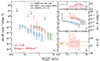 |
Fig. 9. Overdensity of dusty star-forming galaxies in the MQN01. Panel a: differential 1.2 mm continuum source number count density in MQN01 (red points and boxes; including galaxies within |ΔvQSO|< 1000 km s−1), SSA22 (black dots and green boxes; Umehata et al. 2017, 2019 within ±1000 km s−1 of the median source redshift), and in blank fields as derived from ASPECS large program (black points and blue boxes; Aravena et al. 2019, 2020; Boogaard et al. 2019, 2020; González-López et al. 2019, 2020) including sources with spectroscopic redshift between 2.5 ≤ z ≤ 3.5. The downward arrows indicate 1σ upper limits. Panel b: number of sources in each luminosity bin averaged over the iterations. The horizontal gray line reports the total average number of sources entering each bin for the computation of the differential number counts. Panel c: cumulative source number density as a function of 1.2 mm continuum flux obtained by integrating the differential number count density. Panel d: cumulative source overdensity in MQN01 as a function of S1.2 mm. The horizontal lines represent the overdensity range of CO(4–3) emitters in ΔV1000. |
5. Discussion
5.1. The overdensity in MQN01
In Sect. 4.1 we obtained the CO LF in the MQN01 field within |ΔvQSO|< 4000 km s−1 and |ΔvQSO|< 1000 km s−1. The analysis we performed on the data allowed us to estimate the presence of a galaxy overdensity traced by the molecular gas content. We find clear evidence of an overdensity in MQN01 that is a factor of ∼10 − 100 higher than the field, depending on the luminosity cut. The luminosity dependence of the overdensity indicates that the most luminous objects are also the most overabundant. Taking into account all the CO line-detected sources (above the limiting CO(4–3) luminosity  ), we estimated
  in ΔV4000 and
  , counting only secure sources within ΔV1000 without applying the completeness correction. Our results suggest that galaxies in MQN01 field are possibly part of a structure extending within a cosmological volume of at least ∼600 cMpc3 as probed by our ALMA survey.
In addition, we can investigate the normalization and shape of the CO LF in MQN01, which encloses key information on the assembly of galaxies in such an overdense region. However, an accurate analysis of the LF trend and its interpretation is challenging given the low statistics of the sample and large uncertainties. To compare the CO LF in MQN01 with that measured in blank fields, we consider the one computed in ΔV4000 corrected for both the source fidelity and the survey completeness.
The observed CO LF in the MQN01 field can be produced by a combination of an excess in galaxy number counts (thus increasing the overall normalization) and an enhanced CO luminosity of galaxies in the field (which translates to a shift of the source counts toward higher luminosities). However, a pure luminosity shift seems at odds with the data. Indeed, assuming that the CO LF in MQN01 follows the trend expected for blank fields (typically fit by a Schechter function; Schechter 1976), there is evidence for a further excess at the high-luminosity end producing a flattening at  , which is also reflected in an increase in the cumulative overdensity values, δ(>
  ), reported in Fig. 8. Interestingly, this excess is even more evident when considering the “raw” CO LF within ΔV1000. To demonstrate this fact, in Fig. 8 we report the rescaled version of the best-fit model to blank field data and the result obtained from the SIDES simulation. If the observed flattening at the high-luminosity tail of the LF is ascribed to a systematical increase in galaxy CO(4–3) luminosities, this can be due to either a higher galaxy molecular gas budget or enhanced molecular gas excitation in turn due to significant star-formation activity and/or a higher AGN fraction in the field, which can increase the fraction of molecules populating higher-J CO states without necessary increasing the bulk of the CO-traced molecular gas mass. In the first scenario, if such galaxies follow the Kennicutt–Schmidt relation (Schmidt 1959; Kennicutt 1998; Kennicutt & Evans 2012, for a review), this would imply that galaxy assembly is accelerated in this dense field with more massive galaxies experiencing considerable episodes of star formation. Regarding the second possible scenario, the sole detection of CO(4–3) is not sufficient to determine the dominant physical mechanism responsible for the molecular gas excitation. A proper sampling of multiple CO rotational ladders is therefore needed to understand if there is an important contribution to the enhancement of the CO(4–3) luminosity from high star-formation activity or X-ray radiation from AGN (see, e.g., Wolfire et al. 2022, for a review). Interestingly, four out of seven (≃57%) of the CO-detected sources in |ΔvQSO|< 1000 km s−1 are also detected in the X-rays, thus suggesting an intense AGN activity in the field (Travascio et al., in prep.). Highly excited molecular gas and high star-formation efficiency have been found in the core of protoclusters at high z (see, e.g., Lee et al. 2017; Coogan et al. 2018). However, since the aforementioned effects are interlaced, we are hampered in drawing strong conclusions here. Further information can be obtained by evaluating the star-formation rate of the selected CO line-emitting galaxies, which is possible in the millimeter regime by measuring the galaxy FIR luminosities (see, e.g., De Looze et al. 2014). However, our observations provide us with at best two different photometric measurements in the Rayleigh-Jeans tail of the dust spectral energy distribution, therefore preventing a proper estimation of the LFIR without an a priori assumption on the galaxy dust temperature (Tdust).
The comparison of the CO LFs is based on the evaluation of differential number counts, which are likely to be affected by Poissonian statistical oscillations. The cumulative LF, nCO(> L′), can mitigate the uncertainties, providing a more robust result. Here, the flattening that occurs at  is less sharp. However, there is a hint of a shallower decline of nCO with respect to blank fields.
We can then ask if the overdensity revealed in MQN01 via CO line emission is different from that revealed by other tracers. In Sect. 4.2, we analyzed the 1.2 mm source number count density in MQN01 within |ΔvQSO|< 1000 km s−1, and we compared it with those of blank fields by selecting a sample of galaxies between 2.5 ≤ z ≤ 3.5 from ASPECS large program (see Aravena et al. 2019, 2020; Boogaard et al. 2019, 2020; González-López et al. 2019, 2020). This comparison yields an overdensity signal that is also on the order of 10–100 depending on the flux cut (see Fig. 9). We stress that such an analysis is affected by large uncertainties due to low statistics of the selected samples. In addition, the selection of galaxies that are detected in their rest-frame submillimeter dust continuum emission and for which spectroscopic redshift information is available from different lines can introduce biases that are difficult to assess (see Sect. 4.2 for further details). Any interpretation here should therefore be taken with caution. Given the above limitations, an analysis of the source number count trend as a function of continuum flux density cannot be performed. Notwithstanding, we argue that overdensity traced by dust continuum is consistent with what we found from the analysis of CO LFs. The source number counts shown of MQN01 in Fig. 9 do not exhibit any evidence of a flattening as observed in the CO LF, and can therefore be interpreted as a pure normalization effect with respect to those of blank fields. However, the 1.2 mm flux density at z ∼ 3 (corresponding to ∼300 μm rest-frame wavelength) probes the Rayleigh-Jeans tail of the FIR dust emission, which scales as ∼MdustTdust (see, e.g., Hodge & da Cunha 2020). Therefore, any possible contribution to increasing the observed 1.2 mm flux density in galaxies located in the MQN01 volume cannot be directly attributed to either warmer dust temperature or a larger amount (Mdust) of cold dust in galaxies. We also compare the observed 1.2 mm number counts with that toward the SSA22 protocluster at z ∼ 3 (Umehata et al. 2017, 2019) obtained via a survey with similar design as we present here. The spectroscopic redshift information of galaxies in SSA22 are obtained through the measurement of CO(3–2) line thus providing a fair comparable sample. At zeroth order, the differential and cumulative number counts in MQN01 field are consistent with what has been found in SSA22 field. This evidence possibly suggests that similar physical mechanisms are caught in actions in these environments (we further discuss this point in Sect. 5.3).
5.2. Molecular gas density in the MQN01 field
We estimated the total molecular gas content in the MQN01 structure by summing up the molecular gas masses of galaxies within the structure. To do so, we followed the recipe from Decarli et al. (2016) and Jin et al. (2021):
![Mathematical equation: $$ \begin{aligned} \rho (\mathrm{H_{2}})\left[ M_{\odot }\mathrm{\,cMpc^{-3}} \right] = \frac{1}{\Delta V}\sum _{i}M_{\rm H_{2}}^{i}\frac{F_{i}}{C_{i}}, \end{aligned} $$](/articles/aa/full_html/2024/04/aa48659-23/aa48659-23-eq124.gif) (8)
(8)
where MH2 is the galaxy molecular gas mass. To estimate MH2 for each galaxy, we have to assume a CO(4–3)-to-CO(1–0) conversion factor ( ) and an αCO coefficient (
 ; see Bolatto et al. 2013, for a review). Such parameters are unknown for our CO(4–3) emitters in the MQN01 field. We adopted r41 = 0.61 ± 0.13 obtained via modeling of the CO ladders of sources at z = 2.0 − 2.7 in the ASPECS field (see Boogaard et al. 2020, and references therein). The typical values of αCO adopted in the literature vary from 0.8 M⊙ (K km s−1 pc2)−1 for local ultra-luminous infrared galaxies, SMGs, and quasar hosts (Downes & Solomon 1998 but see also Montoya Arroyave et al. 2023 who measured a higher average value of 1.7 ± 0.5 M⊙ (K km s−1 pc2)−1 for local (ultra-)luminous infrared galaxies), to ∼4 M⊙ (K km s−1 pc2)−1 for the giant molecular clouds in the Milky Way (see, e.g., Bolatto et al. 2013; Carilli & Walter 2013, for further discussion). To take into account all the uncertainties, we computed ρ(H2) by performing a Monte Carlo simulation by varying all the measurements within their uncertainties. For the source fidelity and completeness, we adopted the same approach as in the evaluation of the CO LFs and continuum number counts (see Sects. 4.1 and 4.2). During the simulation, we also accounted for the uncertainty on r41, and we varied αCO/(M⊙ (K km s−1 pc2)−1) uniformly in the range 0.8 − 4.3. This procedure yields
  , where the nominal values and uncertainties are computed by taking the 50th, 5th, and 95th percentile, respectively. Similarly, we computed the molecular gas density for galaxies within |ΔvQSO|< 1000 km s−1 ignoring completeness corrections and we obtained ρ(H2) = (1.0 ± 0.3)×109 M⊙ cMpc−3.
In Fig. 10 we compare our results with the molecular gas density across cosmic time in blank fields as reported by several works in the literature. We report results from the CO Luminosity Density at High Redshift (COLDz; Pavesi et al. 2018; Riechers et al. 2019), ASPECS (Decarli et al. 2019, 2020), the Very Large Array (VLA)–ASPECS (VLASPECS; Riechers et al. 2020), Institute for Radio Astronomy in the Millimeter Range (IRAM) Plateau de Bure High-z Blue Sequence Survey 2 (PHIBBS2; Freundlich et al. 2019; Lenkić et al. 2020), the NOEMA survey in the HDF-N (Boogaard et al. 2023), and the xCOLD GASS survey (Saintonge et al. 2011, 2017; Fletcher et al. 2021). We also report measurements of the cosmic molecular gas density obtained via the dust continuum surveys (see Berta et al. 2013; Scoville et al. 2017; Magnelli et al. 2020), as well as the best fit to data obtained from Walter et al. (2020). We found that the molecular gas budget residing in MQN01 is ∼10× the expected molecular gas density at z ∼ 3 consistent with what we found from the analysis of the CO LF. This corroborates our findings indicating that galaxies in MQN01 are evolving in a gas-rich overdense environment.
 |
Fig. 10. Molecular gas density in the MQN01 field for galaxies within |ΔvQSO|< 1000 km s−1 (red star) compared to results in blank fields from HDF-N+ASPECS-LP (Boogaard et al. 2023), ASPECS-LP (Decarli et al. 2019, 2020), PHIBBS2 (Lenkić et al. 2020), COLDz (Riechers et al. 2019), VLASPECS (Riechers et al. 2020), and the xCOLD GASS survey (Fletcher et al. 2021). We also report measurements of the cosmic molecular gas density obtained via dust continuum (gray bars; Berta et al. 2013; Scoville et al. 2017; Magnelli et al. 2020) and the best-fitting function from Walter et al. (2020). The green symbol is the molecular gas density in the Spiderweb protocluster (Jin et al. 2021). |
We also compare our result with that obtained in the Spiderweb protocluster at z = 2.16 reported by Jin et al. (2021,  ) as traced by CO(1–0). The emission from this line is a more direct proxy (because it does not require assumptions on the CO line excitation) of the molecular gas mass in galaxies (though it still requires an assumption on the αCO luminosity-to-H2 mass conversion factor). Jin et al. (2021) adopted two typical values of αCO/(M⊙ (K km s−1 pc2)−1) for their sources equal to 0.8 for starburst-like objects (Emonts et al. 2018) and 3.6 for disk-like galaxies (Daddi et al. 2010). We note here that millimeter observations toward the Spiderweb protocluster probed a much larger volume (∼6600 cMpc3) with respect to our ALMA survey in the MQN01 field. However, our measurements point to a molecular mass density that is comparable to that found in one of the most massive protoclusters at later times.
5.3. Comparison with (sub)millimeter surveys of high-z protoclusters
Comparing our findings with results obtained in other fields hosting high-z galaxy-rich environments would allow us to place our results into a wider context. However, this is somehow difficult since a fair comparison requires at least a similar survey design at comparable redshift. Indeed, the observed galaxy population strongly depends on the observed tracers, selection method, sensitivity, and area of the survey. In our work we find a peculiar feature in the CO LF that suggests a flattening at the bright end relative to the trend expected in blank fields. Despite numerous works in the literature reporting CO surveys in overdense environments (see Sect. 1), a systematic analysis of the CO LF in such environments across the redshift range is still missing. Jin et al. (2021) report a large area (∼21 arcmin2) survey of CO(1–0) with the Australia Telescope Compact Array (ATCA) toward the Spiderweb protocluster at z = 2.16. By using 46 identified CO emitters, they put a first constraint of the CO(1–0) LF in a protocluster environment. By fitting the data using a Schechter function with a fixed slope as determined by studies in blank fields (such as COLDz; see Riechers et al. 2019), they find a CO(1–0) LF normalization that is ∼1.5 dex higher than that in fields. Interestingly, the CO(1–0) LF reported by Jin et al. (2021), does not seems to show any signature of flattening at its bright end, even when considering a small volume (∼1650 cMpc3) centered around the starbursting radio galaxy MRC1138-262 (see, e.g., Miley et al. 2006; Emonts et al. 2016) where the highest concentration of galaxies has been found.
Another attempt to study the LF in high-z protocluster field is reported by Hill et al. (2020), who present ALMA follow-up observations of SPT2349-56, a star-forming protocluster core at z = 4.3, targeting the CO(4–3) as well as the singly ionized carbon fine-structure line [CII]158 μm. They reveal 24 line-emitting sources in ∼7.2 arcmin2, through which they obtain the FIR and [CII]158 μm luminosity differential number counts. Intriguingly, they find that the FIR LF in the core of SPT2349-56 is biased toward bright galaxies compared to what is predicted for field galaxies, thus suggesting an enhanced star-formation activity possibly triggered by ongoing mergers (see, e.g., Tacconi et al. 2008; Engel et al. 2010; Luo et al. 2015), which are expected to be more common in overdense regions (see, e.g., Lotz et al. 2013; Hine et al. 2016). On the basis of the almost-linear CO-FIR luminosity relation (see, e.g., Liu et al. 2015; Kamenetzky et al. 2016) this would directly translate in an increased  luminosity at the bright end of the CO LF as we observe in the MQN01 field.
A comparable example to our observations is the SSA22 field, a protocluster at z ≃ 3.1 surveyed by Umehata et al. (2015, 2017) with ALMA achieving a sensitivity of ∼60 μJy beam−1 over an area of ∼2′×3′ probing the galaxy dust continuum at 1.1 mm. Therefore, this survey is fairly comparable to our work both in terms of survey design and redshift. Umehata et al. (2018, 2019) followed-up this field by extending both the probed area and including CO(3–2) line observations using ALMA band 3. In the combined survey, Umehata et al. (2018) report the detection of 35 SMGs and the 1.1 mm number counts, which reveal an excess by a factor of several with respect to blank field. In this work we combined data from Umehata et al. (2018, 2019), and we rescaled the observed fluxes to 1.2 mm at z = 3.25 (see Sect. 4.2). The source number counts in MQN01 and SSA22 appear to be overlapped following a similar trend (albeit with large uncertainties). This might indicate that dust-obscured star formation and metal production in galaxies in MQN01 field are enhanced in the protocluster. In addition, we conclude that the galaxy density as traced by the 1.2 mm dust continuum emission in MQN01 is comparable to that revealed in SSA22 field.
5.4. Is MQN01 a protocluster in formation?
5.4.1. Galaxy velocity distribution
In Fig. 11 we report the distribution of ΔvQSO of the combined ALMA+MUSE sample, including sources with high-fidelity spectroscopic redshift within |ΔvQSO|< 4000 km s−1. Interestingly, we can identify a “core” population of galaxies having |ΔvQSO|< 1000 km s−1 that appear to be Gaussian distributed as expected for cluster (i.e., virialized) galaxies (see, e.g., Yahil & Vidal 1977), with the distribution median value appearing slightly shifted with respect to the QSO systemic redshift of ∼ − 200 km s−1. To test this hypothesis, in Fig. 11 (blue bins) we additionally report the (cumulative) velocity distribution of galaxies belonging to |ΔvQSO|< 1000 km s−1, within the estimated core virial radius of Rvir ∼ 100 kpc (see Sect. 5.4.2). We therefore tested the Gaussianity of the sample by performing a Lilliefors test (Lilliefors 1967)14 and obtained a p-value of 0.94. Therefore, we do not have the significance level to reject the null hypothesis, and the small number statistics prevent any strong conclusion in this case. The mean velocity and the standard deviation of the core galaxies is  and
and  ; the uncertainties were computed using bootstrap resampling. In Fig. 11 we report the theoretical cumulative Gaussian, which reproduces the observed velocity distribution of the core galaxies fairly well.
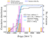 |
Fig. 11. Distributions of galaxy line-of-sight velocities in the MQN01 field. Right axis: Velocity distribution of galaxies in the MQN01 field either detected in their CO(4–3) lines in our ALMA band 6 survey (orange bins) or having high-fidelity spectroscopic redshift within |ΔvQSO|< 4000 km s−1 measured from MUSE data (violet bins). The blue hatched bins are the distribution of galaxy velocities in the core. Left axis: Cumulative distribution of the whole sample and that of the core (black and blue lines, respectively). The light blue curve is the theoretical prediction for a Gaussian distribution of velocities with central value and dispersion as reported in the legend. The gray band represents the 1σ confidence interval. |
5.4.2. Halo mass estimate
Under the assumption that the observed galaxies in the core of MQN01 field are virialized within a large dark matter (DM) halo (see, e.g., Miller et al. 2018; Hill et al. 2020), we can estimate the total halo mass on the basis of the observed velocity dispersion of the galaxies. To do so, we employed the scaling relation found by Evrard et al. (2008, see also Rines et al. 2013), which is based on a suite of N-body simulations with various cosmologies:
 (9)
(9)
where h(z) = H(z)/100 km s−1 Mpc−1 and σr is the line-of-sight velocity dispersion of the halo members.
To define the halo members, we proceeded iteratively. We took all galaxies within |ΔvQSO|< 1000 km s−1, and we computed the dispersion of the line-of-sight velocity of galaxies (assuming they are due to purely peculiar motion) and the average position of the galaxies (i.e., the geometrical barycenter projected on the sky plane)15. We therefore computed M200 using Eq. (9) and the virial radius (R200 ≡ Rvir) as Rvir = [GM200/(100 H(z)2)]1/3. We then iterated the procedure by selecting all galaxies within Rvir until convergence. By doing so, we determined a total dynamical halo mass of  and a virial radius of
  , where the nominal values and uncertainties are computed with a Monte Carlo sampling and by taking the 5th, 50th, and 95th percentile of the distribution. However, we note that such estimates involve a set of assumptions and therefore have to be taken with caution. In particular, we have assumed that the halo is spherical and that thus the velocity dispersion can be simply derived from the line-of-sight velocity. However, numerical simulations show that halos are likely to be triaxial spheroids whose axis ratios depends on halo mass and that the line-of-sight velocity, on average, underestimate the dispersion but has significant scatter (see, e.g., Elahi et al. 2018a,b). Also, the kinematical analysis of cosmological simulations presented by de Beer et al. (2023) suggests significant variations of the line-of-sight velocity of substructures within halos, due to asymmetries in matter accretion. Taken at face value, the mass estimate above would suggest that the host halo of the MQN01 quasar should be similar to the average quasar population at similar redshifts, (i.e., M200 ≃ (1.5 ± 0.5)×1012 M⊙; see de Beer et al. 2023, and references therein). This is somewhat in contrast with the large overdensity of CO emitters found around MQN01 on scales of a few comoving megaparsecs, implying that similar overdensities should have been commonly found around the typical z ∼ 3.5 quasars, unless the MQN01 is a richer structure on larger scales still in the process of merging. In order to test this hypothesis, we estimated the clustering signal in our field as discussed in detail in Appendix B. By fixing the slope of the cross-correlation function to γ = 1.8 as commonly done in the literature at these redshifts (see, e.g., Ouchi et al. 2004; Diener et al. 2017; Fossati et al. 2021; García-Vergara et al. 2022), we find a cross-correlation length for our CO emitters around the QSO CTS G18.01 of
  . However, we stress that the low number counts limits the statistical significance of our results in absolute terms. There are very few other studies in the literature regarding the correlation length of CO emitters around typical quasars at z > 3. By looking at the fields of 17 quasars at z ∼ 3.8 over an area of ≃66″ radius per field, García-Vergara et al. (2022) built a sample of five CO emitters in a velocity window of ±1000 km s−1 above the limiting luminosities (at 5.6σ) that are dependent on distance from the quasars and that typically vary from
  at the center of the field to ≃3.1 × 10¹⁰ K km s−1 pc2 at a distance of ∼1.9 cMpc (rescaled following the PB response of ALMA observations). We notice that our ALMA band 3 mosaic observation does not suffer from the same radial sensitivity dependence. In particular, García-Vergara et al. (2022) find a cross-correlation length of
  (using the same fixed slope of γ = 1.8) and a total overdensity of
  . However, these estimates do not take into account a possible effect on the overdensity on the assumed luminosity cut. Our result shows that the overdensity increases with the CO emitter line luminosity (see Fig. 8). Thus, we expect that a radial dependence of the sensitivity limits would artificially increase the overdensity as a function of radius and thus increasing the correlation length. We can directly test these expectations using our dataset. In particular, in our data we simulated a similar sensitivity radial dependence as described above, obtaining a correlation length of
  which is significantly larger with respect to the previous estimate with uniform sensitivity and with respect to the value found around typical quasars at z ∼ 3.8 by García-Vergara et al. (2022) (albeit consistent within large uncertainties due to the low number statistics). This result suggests that either the MQN01 quasar host halo is much more massive than suggested by the kinematical analysis discussed above or that the quasar is surrounded by a rich structure consisting in multiple massive halos, or both. Ongoing surveys tracing the galaxy population on scales of tens of comoving megaparsecs (Galbiati et al., in prep.) and aimed at characterizing the halos of other galaxies in the field will enable us to solve this dichotomy.
Assuming that the halo mass is consistent with the kinematical analysis above, we can also estimate which galaxies are bound to the core by comparing their line-of-sight velocity as a function of the projected distance from the estimated center of the halo (i.e., the geometrical barycenter of galaxies within the core; see Fig. 12). In particular, we shifted the galaxy velocities by their mean value within the virial radius and rescaled them by  . We also report the escape velocity assuming a central point-like mass
  as well as a more realistic model that is a truncated Navarro-Frenk-White (NFW) mass profile (Navarro et al. 1996)16. Galaxies that fall within the envelope are expected to be gravitationally bound. However, sources that are located well beyond the virial radius are expected to be dragged by the Hubble flow, unless they have significant tangential velocity component toward the halo center. More precisely, galaxies that are expected to escape from the DM halo potential are those located beyond the so-called turnaround radius, which is estimated from numerical simulations to be Rta ≃ 3.3 Rvir (see, e.g., Gunn & Gott 1972; Busha et al. 2003, 2005). This is the situation for a large fraction of galaxies, including 7 out of 11 CO-line emitters in our selected sample. Interestingly, we can identify a galaxy group (which includes sources L01, L02, L03, and L09) that lies within ∼200 − 500 kpc and |Δv| < 1000 km s−1 of the inferred halo center. Such a symmetrical configuration cannot be due to selection effect and it could suggest the existence of a causal connection between the core and a possible larger structure extending out a few hundred kiloparsecs. In particular, L01–L03 and L09 show small line-of-sight velocity and are located close to the turnaround radius, thus suggesting that we are possibly witnessing the moment in which these galaxies are decoupling from the Hubble flow and about to start their infall toward the core of the protocluster. However, we note that sky-projected distances of galaxies from the halo center has to be considered as lower limit to the true distances. Indeed, we expect to see in projection some galaxies having Rsky ∼ Rta with three-dimensional distance R > Rta. These galaxies are physically in the Hubble flow and dynamically disconnected from the protocluster. This possibly explains why some galaxies (in particular several MUSE-selected sources), have a projected distance within (or comparable to) the turnaround radius while exhibiting high line-of-sight velocities consistent with the Hubble flow. Finally, we note that galaxies having large distance from the halo center also tend to show large velocity shifts. This is the case of L05–L08, which are all among the most distant (in the phase space) sources from the protocluster core and for which we do not have an independent redshift confirmation. Hence, if future studies determine that such sources are actually interlopers at different redshifts or false-positive detections, this will not affect the dynamical analysis presented in this work. In conclusion, our analysis suggests that while the core appears to be bound, the entire system is not virialized. This conclusion is further supported by the measured galaxy overdensity considering that a virialized system should have a DM overdensity of around ∼200, which is always smaller than that traced by galaxies (see, e.g., Lacey & Cole 1994; Desjacques et al. 2018).
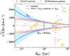 |
Fig. 12. Estimated three-dimensional galaxy velocities (including a statistical correction factor of |

Finally, using the sources associated with the core, we can set a tentative limit of the baryon fraction in molecular form within the halo. We summed up the molecular mass of the individual CO-detected sources within the virial radius (i.e., the QSO, Object B, and L04), which we estimated following the procedure described in Sect. 5.2, assuming αCO = 0.8 M⊙ (K km s−1 pc2)−1 typical of quasar hosts and SMGs (e.g., Downes & Solomon 1998). By doing so, we found  , which is about ∼25% of the total baryon mass of the halo assuming the maximum cosmic baryon fraction of Ωb/Ωm = 0.156 (Planck Collaboration VI 2020). The molecular baryon fraction is therefore
  (assuming the estimated DM halo mass above as a lower limit).
6. Summary and conclusions
We have presented an ALMA survey of the MQN01 field, which hosts a giant Ly-α nebula around a radio-quiet quasar at z = 3.25 (Borisova et al. 2016). Our survey is designed to primarily target the CO(4–3) transition as well as the 1.2 mm (rest-frame ∼300 μm) dust continuum of galaxies in the entire MUSE FoV (∼4 arcmin2). The combination of our FIR observations with the multiwavelength information collected using multiple facilities allowed us to unveil the molecular gas content and the cold dust emission of galaxies in this field. Below, we summarize our main findings:
-
We have identified a robust sample of 11 CO(4–3) emitters within |ΔvQSO|< 4000 km s−1, including a closely separated companion (Object B) located ∼1″ south of the QSO CTS G18.01. Object B was not detected previously in optical data due to its proximity to the QSO. Nine sources (including the QSO) are in the area covered by the MUSE observations, five of which (≃56%, including Object B) do not have any MUSE counterparts. This highlights the crucial role of (sub)millimeter surveys in obtaining a complete census of a galaxy population at high z.
-
Our observations revealed 11 sources through their dust continuum emission observed at 1.2 mm. Five of them (including the QSO and Object B) are also detected in the CO(4–3) line, and another has a MUSE counterpart in the rest-frame UV. This implies the presence of six 1.2 mm-continuum-selected galaxies in a narrow redshift range of |ΔvQSO|< 1000 km s−1.
-
We analyzed the CO(4–3) LFs in the MQN01 field within 2395 cMpc3 (|ΔvQSO|< 4000 km s−1) and 599 cMpc3 (|ΔvQSO|< 1000 km s−1), and we compared them with those of blank fields. We find a systematic excess of galaxy number counts, which points to a galaxy overdensity of
 and
and  above the limiting CO(4–3) luminosity of our ALMA survey. Notably, we find evidence of a flattening at the bright end of the LF with respect to the expected trend in blank fields at similar redshifts. Despite the limited statistics, these results suggest that massive galaxies in dense environments at z ∼ 3 are richer in molecular gas with respect to the field, allowing them to grow faster than their counterparts in average environments.
 -
We obtained the number count densities in MQN01 for sources detected in dust continuum at 1.2 mm that have high-fidelity spectroscopic information from rest-frame UV metal absorptions from MUSE or the CO line. By building a comparison sample for blank fields exploiting ASPECS catalogs, and applying proper k corrections, we found evidence for a systematic excess of source number counts. The overdensity revealed by our ALMA 1.2 mm survey is consistent (within the large uncertainties) with that traced by the molecular gas. Our source number count density is also consistent with that in the SSA22 protocluster at z = 3.1, suggesting that obscured star formation and, consequently, the metal production are similarly enhanced in such overdense environments.
-
We studied the velocity distribution of galaxies in the field by using sources with high-fidelity spectroscopic redshift information from MUSE and the ALMA survey, and we find evidence for a “virialized” structure that might represent the core of a protocluster in formation. Our dynamical analysis yielded a total halo mass of
 , which, however, should be considered a lower limit on the true halo mass for geometrical reasons.
Further efforts are needed to better understand how galaxies are shaped during their evolution in dense environments and to shed light on the galaxy–large-scale structure connection. In particular, in future works we will fully characterize the galaxy population in MQN01 by exploiting our rich multiwavelength dataset, and we will compare the physical properties of galaxies (such as their stellar and dust mass, star formation rates, gas fraction, morphology, and AGN contribution) with those of field galaxies at similar redshifts. This will enable us to better assess the environmental effect on the galaxy assembly in one of the densest region of the Universe discovered so far at z ∼ 3. Through our high-resolution ALMA observations, we will also study the core of the MQN01 structure by characterizing in detail the galaxy morphology and kinematics, in particular those of the QSO host and the closely separated Object B. In future studies, we will also explore the correlation between galaxy properties and the diffuse ionized gas on large scales as probed by the Ly-α line emission. All this work will help us dissect the galaxy assembly processes to address the question of how galaxies get their gas and how this affects the galaxy gas content.
The code is publicly available at the following link: https://github.com/jigonzal/LineSeeker
LINESEEKER estimates the S/N of the source candidates on the basis of the peak flux density per beam.
Thanks to its design, LINESEEKER can also be used to perform a two-dimensional source search in images by simply skipping channel convolution steps.
Such spatial offsets can be produced due to noise fluctuations or differential dust obscuration.
Here we assumed that the recovered line is a Gaussian with the input FWHM.
This method is equivalent of performing Gaussian fit of the line profile along the spectral axis but has the advantage of being more robust against fit failures. It is therefore preferable to estimate the fluxes of a large number of sources.
This approach has been demonstrated to yield consistent results with respect to other commonly used methods, such as a two-dimensional fit of the flux map or aperture photometry.
We measured the noise as the standard deviation of the signal on the whole image.
We additionally verified our results by performing a two-dimensional fit of continuum images by using the CASA task imfit.
The CO emission line of the QSO and Object B is spatially resolved in the high-resolution observations. For them automatically follows ΔF > 1.
As previously mentioned, we did not apply the completeness correction for the CO LF in ΔV1000.
This volume slightly differs from ΔV1000 used in the computation of the CO LF because of the different survey sky area of the ALMA band 6 mosaic from which we extracted the 1.2 mm continuum-emitting candidates.
This test is based on the commonly used Kolmogorov-Smirnov test. Lilliefors test is specifically used to test the null hypothesis that the sample comes from a normally distributed population, when the null hypothesis does not specify the expected value and variance of the normal distribution.
We note that the selected sample of galaxies does not change if we assume as reference velocity the mean redshift of the core sample instead of that of the QSO (see Sect. 5.4.1).
We truncated the NFW gravitational potential at r = Rvir and we kept it Keplerian outside. In this case  for r < Rvir, where
  , Rs = Rvir/c, f(c) = ln(1 + c)−c/(1 + c), K(c) = c/[(1 + c)ln(1 + c)−c], and we assumed a concentration index c = 4 from Rodríguez-Puebla et al. (2016).
Acknowledgments
We thank the anonymous referee for the careful reading of the paper and useful suggestions which improved the manuscript. We thank Dr. Leindert Boogaard for sharing data and providing support in the data analysis process. This paper makes use of the following ALMA data: ADS/JAO.ALMA#2021.1.00793.S. ALMA is a partnership of ESO (representing its member states), NSF (USA) and NINS (Japan), together with NRC (Canada), MOST and ASIAA (Taiwan), and KASI (Republic of Korea), in cooperation with the Republic of Chile. The Joint ALMA Observatory is operated by ESO, AUI/NRAO and NAOJ. This project was supported by the European Research Council (ERC) Consolidator Grant 864361 (CosmicWeb) and by Fondazione Cariplo grant no. 2020-0902. M.M. was supported in part by grant HST-GO-17065. This research made use of Astropy (http://www.astropy.org), a community-developed core Python package for Astronomy (Astropy Collaboration 2013, 2018), NumPy (Harris et al. 2020), SciPy (Virtanen et al. 2020), Matplotlib (Hunter 2007), and Statsmodel (Seabold & Perktold 2010).
References
- Alberts, S., & Noble, A. 2022, Universe, 8, 554 [Google Scholar]
- Aoyama, K., Kodama, T., Suzuki, T. L., et al. 2022, ApJ, 924, 74 [NASA ADS] [CrossRef] [Google Scholar]
- Appenzeller, I., & Rupprecht, G. 1992, Messenger, 67, 18 [NASA ADS] [Google Scholar]
- Aravena, M., Decarli, R., Walter, F., et al. 2016, ApJ, 833, 68 [Google Scholar]
- Aravena, M., Decarli, R., Gónzalez-López, J., et al. 2019, ApJ, 882, 136 [Google Scholar]
- Aravena, M., Boogaard, L., Gónzalez-López, J., et al. 2020, ApJ, 901, 79 [NASA ADS] [CrossRef] [Google Scholar]
- Arrigoni Battaia, F., Chen, C.-C., Fumagalli, M., et al. 2018a, A&A, 620, A202 [NASA ADS] [CrossRef] [EDP Sciences] [Google Scholar]
- Arrigoni Battaia, F., Prochaska, J. X., Hennawi, J. F., et al. 2018b, MNRAS, 473, 3907 [NASA ADS] [CrossRef] [Google Scholar]
- Arrigoni Battaia, F., Chen, C.-C., Liu, H.-Y. B., et al. 2022, ApJ, 930, 72 [NASA ADS] [CrossRef] [Google Scholar]
- Astropy Collaboration (Robitaille, T. P., et al.) 2013, A&A, 558, A33 [NASA ADS] [CrossRef] [EDP Sciences] [Google Scholar]
- Astropy Collaboration (Price-Whelan, A. M., et al.) 2018, AJ, 156, 123 [Google Scholar]
- Balogh, M., Eke, V., Miller, C., et al. 2004, MNRAS, 348, 1355 [Google Scholar]
- Berta, S., Lutz, D., Nordon, R., et al. 2013, A&A, 555, L8 [NASA ADS] [CrossRef] [EDP Sciences] [Google Scholar]
- Béthermin, M., Fudamoto, Y., Ginolfi, M., et al. 2020, A&A, 643, A2 [Google Scholar]
- Béthermin, M., Gkogkou, A., Van Cuyck, M., et al. 2022, A&A, 667, A156 [NASA ADS] [CrossRef] [EDP Sciences] [Google Scholar]
- Bolatto, A. D., Wolfire, M., & Leroy, A. K. 2013, ARA&A, 51, 207 [CrossRef] [Google Scholar]
- Bond, J. R., Kofman, L., & Pogosyan, D. 1996, Nature, 380, 603 [NASA ADS] [CrossRef] [Google Scholar]
- Boogaard, L. A., Decarli, R., González-López, J., et al. 2019, ApJ, 882, 140 [NASA ADS] [CrossRef] [Google Scholar]
- Boogaard, L. A., van der Werf, P., Weiss, A., et al. 2020, ApJ, 902, 109 [NASA ADS] [CrossRef] [Google Scholar]
- Boogaard, L. A., Decarli, R., Walter, F., et al. 2023, ApJ, 945, 111 [NASA ADS] [CrossRef] [Google Scholar]
- Borisova, E., Cantalupo, S., Lilly, S. J., et al. 2016, ApJ, 831, 39 [Google Scholar]
- Boselli, A., & Gavazzi, G. 2006, PASP, 118, 517 [Google Scholar]
- Busha, M. T., Adams, F. C., Wechsler, R. H., & Evrard, A. E. 2003, ApJ, 596, 713 [NASA ADS] [CrossRef] [Google Scholar]
- Busha, M. T., Evrard, A. E., Adams, F. C., & Wechsler, R. H. 2005, MNRAS, 363, L11 [NASA ADS] [Google Scholar]
- Cai, Z., Fan, X., Bian, F., et al. 2017, ApJ, 839, 131 [NASA ADS] [CrossRef] [Google Scholar]
- Cantalupo, S. 2017, in Gas Accretion onto Galaxies, eds. A. Fox& R. Davé, Astrophys. Space Sci. Lib., 430, 195 [Google Scholar]
- Carilli, C. L., & Walter, F. 2013, ARA&A, 51, 105 [NASA ADS] [CrossRef] [Google Scholar]
- Carniani, S., Maiolino, R., De Zotti, G., et al. 2015, A&A, 584, A78 [NASA ADS] [CrossRef] [EDP Sciences] [Google Scholar]
- Casey, C. M., Narayanan, D., & Cooray, A. 2014, Phys. Rep., 541, 45 [Google Scholar]
- Castignani, G., Combes, F., Salomé, P., et al. 2019, A&A, 623, A48 [NASA ADS] [CrossRef] [EDP Sciences] [Google Scholar]
- Champagne, J. B., Casey, C. M., Zavala, J. A., et al. 2021, ApJ, 913, 110 [NASA ADS] [CrossRef] [Google Scholar]
- Chen, C.-C., Arrigoni Battaia, F., Emonts, B. H. C., Lehnert, M. D., & Prochaska, J. X. 2021, ApJ, 923, 200 [NASA ADS] [CrossRef] [Google Scholar]
- Coogan, R. T., Daddi, E., Sargent, M. T., et al. 2018, MNRAS, 479, 703 [NASA ADS] [Google Scholar]
- Cooper, M. C., Newman, J. A., Weiner, B. J., et al. 2008, MNRAS, 383, 1058 [Google Scholar]
- Coppin, K., Chapin, E. L., Mortier, A. M. J., et al. 2006, MNRAS, 372, 1621 [Google Scholar]
- da Cunha, E., Groves, B., Walter, F., et al. 2013, ApJ, 766, 13 [Google Scholar]
- Daddi, E., Bournaud, F., Walter, F., et al. 2010, ApJ, 713, 686 [NASA ADS] [CrossRef] [Google Scholar]
- Darvish, B., Mobasher, B., Sobral, D., et al. 2016, ApJ, 825, 113 [NASA ADS] [CrossRef] [Google Scholar]
- Davis, M., & Geller, M. J. 1976, ApJ, 208, 13 [NASA ADS] [CrossRef] [Google Scholar]
- de Beer, S., Cantalupo, S., Travascio, A., et al. 2023, MNRAS, 526, 1850 [NASA ADS] [CrossRef] [Google Scholar]
- Decarli, R., Walter, F., Aravena, M., et al. 2016, ApJ, 833, 69 [Google Scholar]
- Decarli, R., Walter, F., Gónzalez-López, J., et al. 2019, ApJ, 882, 138 [Google Scholar]
- Decarli, R., Aravena, M., Boogaard, L., et al. 2020, ApJ, 902, 110 [Google Scholar]
- De Looze, I., Cormier, D., Lebouteiller, V., et al. 2014, A&A, 568, A62 [NASA ADS] [CrossRef] [EDP Sciences] [Google Scholar]
- Desjacques, V., Jeong, D., & Schmidt, F. 2018, Phys. Rep., 733, 1 [Google Scholar]
- Diener, C., Wisotzki, L., Schmidt, K. B., et al. 2017, MNRAS, 471, 3186 [NASA ADS] [CrossRef] [Google Scholar]
- Domínguez-Gómez, J., Pérez, I., Ruiz-Lara, T., et al. 2023, Nature, 619, 269 [CrossRef] [Google Scholar]
- Downes, D., & Solomon, P. M. 1998, ApJ, 507, 615 [NASA ADS] [CrossRef] [Google Scholar]
- Dressler, A. 1980, ApJ, 236, 351 [Google Scholar]
- Dressler, A., Oemler, A., Jr., Couch, W. J., et al. 1997, ApJ, 490, 577 [NASA ADS] [CrossRef] [Google Scholar]
- Dunlop, J. S., McLure, R. J., Biggs, A. D., et al. 2017, MNRAS, 466, 861 [Google Scholar]
- Elahi, P. J., Power, C., Lagos, C. d. P., Poulton, R., & Robotham, A. S. G. 2018a, MNRAS, 477, 616 [NASA ADS] [CrossRef] [Google Scholar]
- Elahi, P. J., Welker, C., Power, C., et al. 2018b, MNRAS, 475, 5338 [NASA ADS] [CrossRef] [Google Scholar]
- Elbaz, D., Daddi, E., Le Borgne, D., et al. 2007, A&A, 468, 33 [NASA ADS] [CrossRef] [EDP Sciences] [Google Scholar]
- Emonts, B. H. C., Lehnert, M. D., Villar-Martín, M., et al. 2016, Science, 354, 1128 [NASA ADS] [CrossRef] [Google Scholar]
- Emonts, B. H. C., Lehnert, M. D., Dannerbauer, H., et al. 2018, MNRAS, 477, L60 [NASA ADS] [CrossRef] [Google Scholar]
- Engel, H., Tacconi, L. J., Davies, R. I., et al. 2010, ApJ, 724, 233 [NASA ADS] [CrossRef] [Google Scholar]
- Ester, M., Kriegel, H. P., Sander, J., & Xu, X. 1996, Second International Conference on Knowledge Discovery and Data Mining (KDD’96) (AAAI Press), 226 [Google Scholar]
- Evrard, A. E., Bialek, J., Busha, M., et al. 2008, ApJ, 672, 122 [Google Scholar]
- Fletcher, T. J., Saintonge, A., Soares, P. S., & Pontzen, A. 2021, MNRAS, 501, 411 [Google Scholar]
- Foreman-Mackey, D., Hogg, D. W., Lang, D., & Goodman, J. 2013, PASP, 125, 306 [Google Scholar]
- Fossati, M., Wilman, D. J., Mendel, J. T., et al. 2017, ApJ, 835, 153 [Google Scholar]
- Fossati, M., Fumagalli, M., Lofthouse, E. K., et al. 2021, MNRAS, 503, 3044 [NASA ADS] [CrossRef] [Google Scholar]
- Freundlich, J., Combes, F., Tacconi, L. J., et al. 2019, A&A, 622, A105 [NASA ADS] [CrossRef] [EDP Sciences] [Google Scholar]
- Fujimoto, S., Ouchi, M., Ono, Y., et al. 2016, ApJS, 222, 1 [Google Scholar]
- Fujimoto, S., Kohno, K., Ouchi, M., et al. 2023, ApJS, submitted [arXiv:2303.01658] [Google Scholar]
- García-Vergara, C., Hennawi, J. F., Barrientos, L. F., & Rix, H.-W. 2017, ApJ, 848, 7 [CrossRef] [Google Scholar]
- García-Vergara, C., Hennawi, J. F., Barrientos, L. F., & Arrigoni Battaia, F. 2019, ApJ, 886, 79 [CrossRef] [Google Scholar]
- García-Vergara, C., Rybak, M., Hodge, J., et al. 2022, ApJ, 927, 65 [CrossRef] [Google Scholar]
- Gehrels, N. 1986, ApJ, 303, 336 [Google Scholar]
- Gkogkou, A., Béthermin, M., Lagache, G., et al. 2023, A&A, 670, A16 [NASA ADS] [CrossRef] [EDP Sciences] [Google Scholar]
- Gómez, P. L., Nichol, R. C., Miller, C. J., et al. 2003, ApJ, 584, 210 [Google Scholar]
- Gómez-Guijarro, C., Riechers, D. A., Pavesi, R., et al. 2019, ApJ, 872, 117 [CrossRef] [Google Scholar]
- González-López, J., Bauer, F. E., Romero-Cañizales, C., et al. 2017a, A&A, 597, A41 [NASA ADS] [CrossRef] [EDP Sciences] [Google Scholar]
- González-López, J., Bauer, F. E., Aravena, M., et al. 2017b, A&A, 608, A138 [NASA ADS] [CrossRef] [EDP Sciences] [Google Scholar]
- González-López, J., Decarli, R., Pavesi, R., et al. 2019, ApJ, 882, 139 [Google Scholar]
- González-López, J., Novak, M., Decarli, R., et al. 2020, ApJ, 897, 91 [Google Scholar]
- Guaita, L., Francke, H., Gawiser, E., et al. 2013, A&A, 551, A93 [NASA ADS] [CrossRef] [EDP Sciences] [Google Scholar]
- Gullberg, B., Lehnert, M. D., De Breuck, C., et al. 2016, A&A, 591, A73 [NASA ADS] [CrossRef] [EDP Sciences] [Google Scholar]
- Gunn, J. E., & Gott, J. R., III 1972, ApJ, 176, 1 [Google Scholar]
- Harris, C. R., Millman, K. J., van der Walt, S. J., et al. 2020, Nature, 585, 357 [NASA ADS] [CrossRef] [Google Scholar]
- Hatsukade, B., Ohta, K., Seko, A., Yabe, K., & Akiyama, M. 2013, ApJ, 769, L27 [NASA ADS] [CrossRef] [Google Scholar]
- Hatsukade, B., Kohno, K., Umehata, H., et al. 2016, PASJ, 68, 36 [NASA ADS] [CrossRef] [Google Scholar]
- Hatsukade, B., Kohno, K., Yamaguchi, Y., et al. 2018, PASJ, 70, 105 [Google Scholar]
- Hayashi, M., Kodama, T., Kohno, K., et al. 2017, ApJ, 841, L21 [NASA ADS] [CrossRef] [Google Scholar]
- Hennawi, J. F., Prochaska, J. X., Cantalupo, S., & Arrigoni-Battaia, F. 2015, Science, 348, 779 [Google Scholar]
- Hill, R., Chapman, S., Scott, D., et al. 2020, MNRAS, 495, 3124 [NASA ADS] [CrossRef] [Google Scholar]
- Hine, N. K., Geach, J. E., Alexander, D. M., et al. 2016, MNRAS, 455, 2363 [NASA ADS] [CrossRef] [Google Scholar]
- Hodge, J. A., & da Cunha, E. 2020, R. Soc. Open Sci., 7, 200556 [NASA ADS] [CrossRef] [Google Scholar]
- Hodge, J. A., Carilli, C. L., Walter, F., Daddi, E., & Riechers, D. 2013, ApJ, 776, 22 [Google Scholar]
- Hogg, D. W., & Turner, E. L. 1998, PASP, 110, 727 [NASA ADS] [CrossRef] [Google Scholar]
- Hogg, D. W., Blanton, M. R., Brinchmann, J., et al. 2004, ApJ, 601, L29 [NASA ADS] [CrossRef] [Google Scholar]
- Hunter, J. D. 2007, Comput. Sci. Eng., 9, 90 [NASA ADS] [CrossRef] [Google Scholar]
- Hunter, T. R., Indebetouw, R., Brogan, C. L., et al. 2023, PASP, 135, 074501 [NASA ADS] [CrossRef] [Google Scholar]
- Ideue, Y., Nagao, T., Taniguchi, Y., et al. 2009, ApJ, 700, 971 [CrossRef] [Google Scholar]
- Ito, K., Kashikawa, N., Toshikawa, J., et al. 2020, ApJ, 899, 5 [NASA ADS] [CrossRef] [Google Scholar]
- Jin, S., Dannerbauer, H., Emonts, B., et al. 2021, A&A, 652, A11 [NASA ADS] [CrossRef] [EDP Sciences] [Google Scholar]
- Kamenetzky, J., Rangwala, N., Glenn, J., Maloney, P. R., & Conley, A. 2016, ApJ, 829, 93 [Google Scholar]
- Kauffmann, G., White, S. D. M., Heckman, T. M., et al. 2004, MNRAS, 353, 713 [Google Scholar]
- Kawinwanichakij, L., Papovich, C., Quadri, R. F., et al. 2017, ApJ, 847, 134 [NASA ADS] [CrossRef] [Google Scholar]
- Kennicutt, R. C., Jr. 1998, ApJ, 498, 541 [Google Scholar]
- Kennicutt, R. C., & Evans, N. J. 2012, ARA&A, 50, 531 [NASA ADS] [CrossRef] [Google Scholar]
- Kovács, A., Chapman, S. C., Dowell, C. D., et al. 2006, ApJ, 650, 592 [CrossRef] [Google Scholar]
- Lacey, C., & Cole, S. 1994, MNRAS, 271, 676 [Google Scholar]
- Lee, M. M., Tanaka, I., Kawabe, R., et al. 2017, ApJ, 842, 55 [CrossRef] [Google Scholar]
- Lenkić, L., Bolatto, A. D., Förster Schreiber, N. M., et al. 2020, AJ, 159, 190 [CrossRef] [Google Scholar]
- Lewis, I., Balogh, M., De Propris, R., et al. 2002, MNRAS, 334, 673 [NASA ADS] [CrossRef] [Google Scholar]
- Lilliefors, H. W. 1967, J. Am. Stat. Assoc., 62, 399 [CrossRef] [Google Scholar]
- Liu, D., Gao, Y., Isaak, K., et al. 2015, ApJ, 810, L14 [NASA ADS] [CrossRef] [Google Scholar]
- Lotz, J. M., Papovich, C., Faber, S. M., et al. 2013, ApJ, 773, 154 [NASA ADS] [CrossRef] [Google Scholar]
- Luo, B., Brandt, W. N., Hall, P. B., et al. 2015, ApJ, 805, 122 [Google Scholar]
- Madau, P., & Dickinson, M. 2014, ARA&A, 52, 415 [Google Scholar]
- Magnelli, B., Boogaard, L., Decarli, R., et al. 2020, ApJ, 892, 66 [NASA ADS] [CrossRef] [Google Scholar]
- Manning, S. M., Casey, C. M., Zavala, J. A., et al. 2022, ApJ, 925, 23 [CrossRef] [Google Scholar]
- Maza, J., Wischnjewsky, M., Antezana, R., & González, L. E. 1995, Rev. Mex. Astron. Astrofis., 31, 119 [Google Scholar]
- McMullin, J. P., Waters, B., Schiebel, D., Young, W., & Golap, K. 2007, in Astronomical Data Analysis Software and Systems XVI, eds. R. A. Shaw, F. Hill, & D. J. Bell, ASP Conf. Ser., 376, 127 [Google Scholar]
- McNamara, B. R., & Nulsen, P. E. J. 2012, New J. Phys., 14, 055023 [NASA ADS] [CrossRef] [Google Scholar]
- Miley, G. K., Overzier, R. A., Zirm, A. W., et al. 2006, ApJ, 650, L29 [NASA ADS] [CrossRef] [Google Scholar]
- Miller, T. B., Chapman, S. C., Aravena, M., et al. 2018, Nature, 556, 469 [CrossRef] [Google Scholar]
- Montoya Arroyave, I., Cicone, C., Makroleivaditi, E., et al. 2023, A&A, 673, A13 [NASA ADS] [CrossRef] [EDP Sciences] [Google Scholar]
- Muzahid, S., Schaye, J., Marino, R. A., et al. 2020a, MNRAS, 498, 4424 [NASA ADS] [CrossRef] [Google Scholar]
- Muzahid, S., Schaye, J., Marino, R. A., et al. 2020b, MNRAS, 496, 1013 [Google Scholar]
- Muzahid, S., Schaye, J., Cantalupo, S., et al. 2021, MNRAS, 508, 5612 [NASA ADS] [CrossRef] [Google Scholar]
- Muzzin, A., Wilson, G., Yee, H. K. C., et al. 2012, ApJ, 746, 188 [Google Scholar]
- Navarro, J. F., Frenk, C. S., & White, S. D. M. 1996, ApJ, 462, 563 [Google Scholar]
- Noble, A. G., McDonald, M., Muzzin, A., et al. 2017, ApJ, 842, L21 [Google Scholar]
- Noble, A. G., Muzzin, A., McDonald, M., et al. 2019, ApJ, 870, 56 [Google Scholar]
- Nowotka, M., Chen, C.-C., Battaia, F. A., et al. 2022, A&A, 658, A77 [NASA ADS] [CrossRef] [EDP Sciences] [Google Scholar]
- Oemler, A., Jr. 1974, ApJ, 194, 1 [NASA ADS] [CrossRef] [Google Scholar]
- Oteo, I., Ivison, R. J., Dunne, L., et al. 2018, ApJ, 856, 72 [Google Scholar]
- Ouchi, M., Shimasaku, K., Okamura, S., et al. 2004, ApJ, 611, 685 [NASA ADS] [CrossRef] [Google Scholar]
- Park, C., Choi, Y.-Y., Vogeley, M. S., et al. 2007, ApJ, 658, 898 [Google Scholar]
- Pavesi, R., Sharon, C. E., Riechers, D. A., et al. 2018, ApJ, 864, 49 [Google Scholar]
- Pedregosa, F., Varoquaux, G., Gramfort, A., et al. 2011, J. Mach. Learn. Res., 12, 2825 [Google Scholar]
- Peng, Y.-j., Lilly, S. J., Kovač, K., et al. 2010, ApJ, 721, 193 [NASA ADS] [CrossRef] [Google Scholar]
- Pérez-Martínez, J. M., Dannerbauer, H., Kodama, T., et al. 2023, MNRAS, 518, 1707 [Google Scholar]
- Pike, S. R., Kay, S. T., Newton, R. D. A., Thomas, P. A., & Jenkins, A. 2014, MNRAS, 445, 1774 [NASA ADS] [CrossRef] [Google Scholar]
- Planck Collaboration VI. 2020, A&A, 641, A6 [NASA ADS] [CrossRef] [EDP Sciences] [Google Scholar]
- Polletta, M., Dole, H., Martinache, C., et al. 2022, A&A, 662, A85 [NASA ADS] [CrossRef] [EDP Sciences] [Google Scholar]
- Postman, M., & Geller, M. J. 1984, ApJ, 281, 95 [Google Scholar]
- Postman, M., Franx, M., Cross, N. J. G., et al. 2005, ApJ, 623, 721 [Google Scholar]
- Quadri, R. F., Williams, R. J., Franx, M., & Hildebrandt, H. 2012, ApJ, 744, 88 [NASA ADS] [CrossRef] [Google Scholar]
- Remijan, A., Biggs, A., Cortes, P. A., et al. 2019, ALMA Technical Handbook, ALMA Doc. 7.3, ver. 1.1 [Google Scholar]
- Riechers, D. A., Pavesi, R., Sharon, C. E., et al. 2019, ApJ, 872, 7 [Google Scholar]
- Riechers, D. A., Boogaard, L. A., Decarli, R., et al. 2020, ApJ, 896, L21 [NASA ADS] [CrossRef] [Google Scholar]
- Rigby, J., Perrin, M., McElwain, M., et al. 2023, PASP, 135, 048001 [NASA ADS] [CrossRef] [Google Scholar]
- Rines, K., Geller, M. J., Diaferio, A., & Kurtz, M. J. 2013, ApJ, 767, 15 [NASA ADS] [CrossRef] [Google Scholar]
- Rodríguez-Puebla, A., Behroozi, P., Primack, J., et al. 2016, MNRAS, 462, 893 [CrossRef] [Google Scholar]
- Rudnick, G., Hodge, J., Walter, F., et al. 2017, ApJ, 849, 27 [NASA ADS] [CrossRef] [Google Scholar]
- Saintonge, A., Kauffmann, G., Kramer, C., et al. 2011, MNRAS, 415, 32 [NASA ADS] [CrossRef] [Google Scholar]
- Saintonge, A., Catinella, B., Tacconi, L. J., et al. 2017, ApJS, 233, 22 [Google Scholar]
- Schechter, P. 1976, ApJ, 203, 297 [Google Scholar]
- Schmidt, M. 1959, ApJ, 129, 243 [NASA ADS] [CrossRef] [Google Scholar]
- Scott, S. E., Fox, M. J., Dunlop, J. S., et al. 2002, MNRAS, 331, 817 [CrossRef] [Google Scholar]
- Scoville, N., Lee, N., Vanden Bout, P., et al. 2017, ApJ, 837, 150 [Google Scholar]
- Seabold, S., & Perktold, J. 2010, 9th Python in Science Conference [Google Scholar]
- Shimakawa, R., Kodama, T., Hayashi, M., et al. 2018, MNRAS, 473, 1977 [NASA ADS] [CrossRef] [Google Scholar]
- Smail, I., Dudzevičiūtė, U., Stach, S. M., et al. 2021, MNRAS, 502, 3426 [NASA ADS] [CrossRef] [Google Scholar]
- Smail, I., Dudzevičiūtė, U., Gurwell, M., et al. 2023, ApJ, 958, 36 [NASA ADS] [CrossRef] [Google Scholar]
- Solomon, P. M., Downes, D., Radford, S. J. E., & Barrett, J. W. 1997, ApJ, 478, 144 [NASA ADS] [CrossRef] [Google Scholar]
- Stach, S. M., Swinbank, A. M., Smail, I., et al. 2017, ApJ, 849, 154 [NASA ADS] [CrossRef] [Google Scholar]
- Steidel, C. C., Adelberger, K. L., Dickinson, M., et al. 1998, ApJ, 492, 428 [Google Scholar]
- Steidel, C. C., Adelberger, K. L., Shapley, A. E., et al. 2000, ApJ, 532, 170 [NASA ADS] [CrossRef] [Google Scholar]
- Tacconi, L. J., Genzel, R., Smail, I., et al. 2008, ApJ, 680, 246 [Google Scholar]
- Tadaki, K.-i., Kodama, T., Hayashi, M., et al. 2019, PASJ, 71, 40 [NASA ADS] [CrossRef] [Google Scholar]
- Tanaka, M., Goto, T., Okamura, S., Shimasaku, K., & Brinkmann, J. 2004, AJ, 128, 2677 [NASA ADS] [CrossRef] [Google Scholar]
- Taylor, E., Almaini, O., Merrifield, M., et al. 2023, MNRAS, 522, 2297 [NASA ADS] [CrossRef] [Google Scholar]
- Tran, K.-V. H., Papovich, C., Saintonge, A., et al. 2010, ApJ, 719, L126 [CrossRef] [Google Scholar]
- Umehata, H., Tamura, Y., Kohno, K., et al. 2015, ApJ, 815, L8 [Google Scholar]
- Umehata, H., Tamura, Y., Kohno, K., et al. 2017, ApJ, 835, 98 [Google Scholar]
- Umehata, H., Hatsukade, B., Smail, I., et al. 2018, PASJ, 70, 65 [Google Scholar]
- Umehata, H., Fumagalli, M., Smail, I., et al. 2019, Science, 366, 97 [Google Scholar]
- Virtanen, P., Gommers, R., Oliphant, T. E., et al. 2020, Nat. Methods, 17, 261 [Google Scholar]
- Walter, F., Decarli, R., Aravena, M., et al. 2016, ApJ, 833, 67 [Google Scholar]
- Walter, F., Carilli, C., Neeleman, M., et al. 2020, ApJ, 902, 111 [Google Scholar]
- Wang, T., Elbaz, D., Daddi, E., et al. 2016, ApJ, 828, 56 [NASA ADS] [CrossRef] [Google Scholar]
- Wang, T., Elbaz, D., Daddi, E., et al. 2018, ApJ, 867, L29 [NASA ADS] [CrossRef] [Google Scholar]
- Wilkinson, C. L., Pimbblet, K. A., Stott, J. P., Few, C. G., & Gibson, B. K. 2018, MNRAS, 479, 758 [NASA ADS] [Google Scholar]
- Williams, C. C., Labbe, I., Spilker, J., et al. 2019, ApJ, 884, 154 [Google Scholar]
- Williams, C. C., Alberts, S., Spilker, J. S., et al. 2022, ApJ, 929, 35 [NASA ADS] [CrossRef] [Google Scholar]
- Wolfire, M. G., Vallini, L., & Chevance, M. 2022, ARA&A, 60, 247 [NASA ADS] [CrossRef] [Google Scholar]
- Yahil, A., & Vidal, N. V. 1977, ApJ, 214, 347 [NASA ADS] [CrossRef] [Google Scholar]
- Yamada, T., Nakamura, Y., Matsuda, Y., et al. 2012, AJ, 143, 79 [Google Scholar]
- Yamaguchi, Y., Kohno, K., Hatsukade, B., et al. 2019, ApJ, 878, 73 [Google Scholar]
- Zhang, Z.-Y., Papadopoulos, P. P., Ivison, R. J., et al. 2016, R. Soc. Open Sci., 3, 160025 [Google Scholar]
Appendix A: Multiwavelength counterparts of ALMA-selected galaxies
In Fig. A.1 we report 7″ × 7″ postage stamps of galaxies that have no rest-frame UV counterparts in MUSE (Object B, L03) and/or remain undetected in the rest-frame optical in JWST/NIRCam images (i.e., L05, L06, L07, and L08), as well as low-fidelity galaxies in our sample that have been selected by cross-matching the MUSE catalog of spectroscopically confirmed objects (i.e., L09 and C08). Such an analysis capitalizes on our multiwavelength observational campaign (see Sect. 2.3, for full details). In what follows, we report a qualitative discussion on the counterparts of such ALMA-selected galaxies studied in this work.
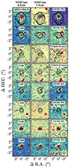 |
Fig. A.1. Postage stamps (7″ × 7″) of some ALMA-selected galaxies. From left to right: JWST/NIRCam F322W2 (3.2 μm), F150W2 (1.5 μm), and the MUSE white-light image. For sources that are located outside the MUSE FoV, we report instead the VLT/FORS2 R-band image. The superimposed black contours show the CO(4–3) line emission or, in the case of C08, the 1.2 mm dust continuum (bottom panels). Contours correspond to [ − 2, 2, 3, 2N]×σ with N, the integer number, >1. |
The high luminosity of the QSO hinders both the optical/UV emission from its host and that of any other closely separated galaxies. A preliminary subtraction of the QSO point spread function in the JWST images reveals the southern Object B in the FW322W2 filter and a possible extended component.
L03 is detected in ALMA CO(4–3) and the millimeter dust continuum (it corresponds to C04 selected with ALMA at 1.2 mm). While unambiguous counterpart is recognizable in the JWST/NIRCam images, especially in the long-wavelength filter, this object remains undetected in the rest-frame UV MUSE white-light image. Notably, the closely separated galaxy located at southeast is a high-confidence MUSE-selected LBGs within |ΔvQSO|< 1000 km s−1. Therefore, these two objects might be located at small physical distance forming an interacting system.
The sources L05, L06, L07, and L08 are detected only in line in our ALMA band 3 mosaic. L05 and L06 lie outside the MUSE footprint, for these objects, in Fig. A.1 we report the rest-frame UV VLT/FORS2 R-band image. As mentioned in Sect. 3.5, these sources might represent either actual false-positive detections or interlopers at different redshifts. We note that a relatively bright source is partially blended in the northwest with the line emission of L07 observed in ALMA. The analysis of the MUSE spectrum unambiguously places the northwest source at z ≃ 0.3358. At this redshift, no common astronomical-observed FIR transitions enters in the ALMA SPW in which we observe the emission line of L07. Therefore, any possible association between the observed line emission in ALMA band 3 and the northwest source can be confidently ruled out.
Finally, L09 and C08 have been selected via the cross-matching between low-fidelity ALMA-selected sources and high-fidelity MUSE-selected LBGs. In Fig. A.1 we show their rest-frame optical/UV counterparts that are well detected in both JWST/NIRCam and VLT/MUSE images.
Appendix B: Clustering analysis
We measured the QSO-CO emitters correlation length following García-Vergara et al. (2017, 2022). We expressed the volume-averaged projected cross-correlation function as
 (B.1)
(B.1)
where ξ(R, Z) is the three-dimensional cross-correlation function ξ(r) = (r/r0)−γ and r0 is the correlation length. In Eq. (B.1) we expressed the cross correlation function in terms of the QSO-galaxy distance components along the plane of the sky (R) and the line of sight (Z), which are related to the three-dimensional distance through r2 = R2 + Z2. To estimate the correlation length in the MQN01 field, we considered all the sources within |ΔvQSO|< 1000 km s−1 = ΔV1000 and we count the QSO-galaxy pairs in cylindrical shells centered on the QSO CTS G18.01. Each volume (Veff) has a depth along the line of sight of ΔZ ≃ (2ΔV1000H(z)−1)(1 + zQSO) (corresponding to ≃25.3 cMpc) and a inner and outer transverse radius of Rmin and Rmax, respectively. We measured χ(R) at angular scales 1″ ≤ θ ≤ 75″ (corresponding to 0.03 ≤ R ≤ 2.4 cMpc at z ≃ 3.25) in logarithmically spaced bins using the following estimator:
 (B.2)
(B.2)
where ⟨QG(Rmin≤R≤Rmax)⟩ and ⟨QR(Rmin≤R≤Rmax)⟩ are the number of QSO–CO-emitter pairs in our survey within the cylindrical shell volume and that expected in absence of clustering at similar redshifts, respectively. The numbers of QSO-CO emitter pairs in MQN01 should then in principle be corrected for the completeness and fidelity of the sources. However, our sample of galaxies within ΔV1000 comprises six objects that are all secure sources with rest-frame optical/UV counterparts (F = 1). Given the large uncertainties involved in this kind of analysis we then opted to do not apply the completeness correction and we assumed that each bin is dominated by Poisson noise for low count statistics (see Gehrels 1986). To estimate the expected source number in blank fields we capitalized on the CO(4–3) LF at z ≃ 3.8 from ASPECS+HDF-N by Boogaard et al. (2023), which is given by a Schechter function with parameters  ,
,  at fixed slope of α = −0.2. The number of expected pairs within a cylindrical shell volume is therefore given by
 (B.3)
(B.3)
where  is the number density of CO(4–3) emitters above a given limiting luminosity (
 ). In our survey, the CO emitters within ΔV1000 are located in regions where our ALMA band 3 mosaic has uniform sensitivity. Therefore, in Eq. (B.3) we take out
  from the integral assuming a constant limiting luminosity at 5σ of
  for line width of FWHM = 331 km s−1 equal to the median line FWHM of the high-fidelity sample of CO(4–3) emitters from González-López et al. (2019). We note that in the computation of ⟨QR(R)⟩ we also took into account the uncertainties on the CO(4–3) LF parameters. We note that this is crucial given that the LF is poorly constrained at its bright end, thus introducing large uncertainties in the computation of the expected source number counts in blank fields. Specifically, we computed different realizations of ⟨QR(R)⟩ for 30 × 30 couples of (log ϕ*, log L*) extracted from random normal distributions with means and standard deviations corresponding to the nominal values and 1σ uncertainties reported by Boogaard et al. (2023), respectively. We then computed the uncertainty on ⟨QR(R)⟩ by taking the 16th and 84th percentile of the distribution.
To determine the three-dimensional cross-correlation length r0, we fit our data by employing the Python MCMC ensemble sampler emcee package (Foreman-Mackey et al. 2013) adopting a Poisson maximum likelihood estimator (see, e.g., Hennawi et al. 2015; García-Vergara et al. 2017) and a fixed slope of γ = 1.8 (see, e.g., Ouchi et al. 2004; Diener et al. 2017; Fossati et al. 2021; García-Vergara et al. 2017, 2019, 2022). In order to properly take into account the uncertainties on the expected source number counts in blank fields, we repeated the fit 900 times by using the different realizations of ⟨QR(R)⟩ computed as described above. We then obtained the final posterior distribution of r0 by summing up all the distributions obtained with this procedure. We finally computed the best-fit r0 value and its 1σ uncertainties by taking the 50th, 16th, and 84th percentile, respectively and obtained  . We report our result in Fig. B.1.
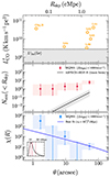 |
Fig. B.1. Estimation of the cross-correlation length in MQN01. Top panel: Source CO line luminosities as a function of radial distance from the central quasar. The gray band shows the 5σ limiting luminosities of our survey (see text for further details). Central panel: Cumulative source number counts in MQN01 (red bins) and that expected in blank fields (black line, with their uncertainties shown in gray). Bottom panel: Projected volume-integrated cross correlation function in MQN01 (blue bins), the best-fit model (solid blue line), and the random draw from our Monte Carlo simulation (in gray). The inset panel shows the posterior distribution of the three-dimensional cross-correlation length with red lines indicating the 16th, 50th, and 84th percentile, respectively. |
There are very few other works in the literature that study the clustering of CO emitters around quasars at z > 3 (e.g., García-Vergara et al. 2022). Some of these works, make use of single-pointing ALMA observations to evaluate the QSO-galaxy cross correlation length using a small sample of CO emitters. In single-pointing observations, the PB response of ALMA antennas introduces a spatial dependence of the sensitivity (and therefore of the limiting luminosity), which therefore decreases radially from the center of the field toward the edge.
We tested the effect of a radial dependence of the limiting luminosity on the evaluation of the correlation length. We repeated the same procedure described above by rescaling our limiting luminosity at 5σ with the PB response of a individual pointing of our ALMA band 3 mosaic modeled as a two-dimensional Gaussian with FWHM = 53.6″ (corresponding to the HPBW at the reference frequency of 108.5 GHz; see Table 1). This yields a higher (areal-averaged) limiting luminosity of  within the last radial annulus at 31.6″ ≤ θ ≤ 75″. In this experiment, sources L03 and L09 would not be detected having
  much below the 5σ limiting luminosity at their sky position and we therefore removed them from the MQN01 source number counts within ΔV1000 (see Table 3). In addition, the number of expected pairs in blank fields decreases in the last radial annulus due to the sharp drop of the CO(4–3) LF at such high luminosities (
 ). The overall effect is an artificial boosting of the χ(R) value in the outer radial bin such that the fit of our data yields a larger best-fit correlation length of
  . This value is still consistent within the large uncertainties with the r0,CO value previously found using the full sample of sources and a uniform limiting luminosities, but with a nominal value that is ∼40% higher. This experiment shows how the variation in the limiting luminosity across the FoV might alter the estimated value of the cross-correlation length in the case of low number statistics.
All Tables
Redshift bin, cosmological volume, and limiting luminosity of the main emission lines entering the USB of our ALMA band 3 survey.
All Figures
|
Fig. 1. Combined PB response for our ALMA mosaics at the representative frequency of 109.0 GHz (band 3, left panel) and for the aggregate continuum mosaic image of ALMA band 6 (right panel). The white contours correspond to a PB response of 30% (solid line) and 50% (dashed line). The circles show the disposition of the pointings with diameter equal to the HPBW of the ALMA 12 m antennas at the reference frequency of the setup. |
| In the text | |
|
Fig. 2. Footprints of our ALMA and MUSE observations toward the MQN01 field. The orange and blue contours encircle the area where the combined mosaic PB response is ≥0.5 for ALMA band 3 and 6, respectively. Within these areas we performed the source search. Violet contour draws the MUSE footprint. The background is a composition of the JWST NIRCam F322W2 image (center and southeast corner) complemented with the VLT/FORS2 R-band observation (northeast, northwest, and southwest corners, and the southeast gap between the JWST NIRCam detectors). The point-spread-function-like emission of QSO CTS G18.01 has been subtracted in the JWST image revealing a nearby southeast quasar companion (Object B). Orange circles and blue squares indicate the locations of the ALMA CO(4–3) line-emitting and 1.2 mm continuum-selected sources in our ALMA band 3 and 6 observations, respectively. Green squares pin-point galaxy candidates detected in continuum at 3 mm in ALMA band 3. Gray hexagons denote sources corresponding to low-z counterparts, all but i5 show bright emission line in ALMA band 3. Violet crosses are the MUSE-selected LBGs belonging within ±1000 km s−1 of the QSO CTS G18.01 systemic redshift. The dashed red circle shows the inner 100 pkpc around the estimated center of the protocluster core. |
| In the text | |
|
Fig. 3. Completeness (red squares, left axis) and flux boosting (blue circles and density plot, right axis) corrected for the PB response as a function of 1.2 mm flux density (bottom axis) and S/N (top axis) of injected sources in the ALMA band 6 continuum image. The error bars are derived by computing the 16th and 84th percentile of the distributions of completeness and flux boosting measurements in each flux bin. The solid red line is the best-fitting function to the completeness values modeled as C(F1.2 mm) = {1 + erf[(F1.2 mm − A)/B]}/2 with A = 0.197 ± 0.004 and B = 0.083 ± 0.007. The density plot shows the values of the flux boosting as a function of the measured flux of the injected sources. |
| In the text | |
|
Fig. 4. Completeness (top panel) and flux boosting (bottom panel) corrected for the PB response as a function of the line-velocity integrated flux and the line FWHM of the injected sources in the ALMA band 3 dirty cube binned at 25 km s−1. In the top panel, the green line indicates where the completeness is ≥90%. |
| In the text | |
|
Fig. 5. Observed frequency of CO and [CI]609 μm transitions as a function of redshift. The boxes encircle both the frequency and redshift ranges covered by our ALMA band 3 observations. Boxes are color-coded by the cosmological volume probed by each transitions. Gray bands show the SPW coverage in the LSB and USB. The mean redshift of transitions entering the USB are also reported. The blue arrow points to the box representing the volume within ±1000 km s−1 around the QSO CTS G18.01 systemic redshift. |
| In the text | |
|
Fig. 6. Spectra of the CO(4–3) line-emitting sources in our ALMA survey of the MQN01 field. The red lines are the best-fit models to the spectra (yellow bins). The green bins indicate the channels we used to compute the line-velocity integrated maps (see Fig. 7) defined within ±2σ of the best-fitting Gaussian line. The horizontal gray bands are the rms noise in each channel. The blue vertical line indicate the QSO CTS G18.01 systemic velocity. Sources are labeled according to the IDCO reported in Table 3. |
| In the text | |
|
Fig. 7. Maps of the ALMA-selected galaxies in the MQN01 field detected in their CO(4–3) line, in the continuum at 1.2 mm, or in both. The color scale at the top refers to line-velocity integrated maps for all sources except C08, which is only detected at 1.2 mm in the dust continuum (bottom right color scale). Solid gray and black contours correspond to the velocity-integrated and 1.2 mm dust continuum maps, respectively and scales as [2, 3, 2N]×σ with N > 1 integer number. Dotted contours are the −2σ level. The yellow ellipse drawn in the bottom right corner represents the FWHM of the synthesized beam of the ALMA band 3 (yellow fill and gray line) and 6 (black line) observations. Sources are labeled according to the IDCO and/or ID1.2 mm reported in Table 3. Sources with spectroscopic-redshift confirmation are marked with a violet square in the upper-left corner. |
| In the text | |
|
Fig. 8. Overdensity of CO emitters in the MQN01 field. Panel a: CO(4–3) LF in MQN01 and in blank fields. The (dark/light) red dots and boxes represent the CO LF in MQN01 field (fidelity (F) + completeness (C)-corrected/uncorrected, respectively) in ΔV4000, while gold hatched boxes are the uncorrected (raw) CO LF within ΔV1000. The blue and green boxes with black dots are data from ASPECS and HDF-N, respectively, which are representative of blank fields at these redshifts (e.g., Decarli et al. 2019, 2020; Boogaard et al. 2023). The downward arrows indicate 1σ upper limits. The dashed black line is the best-fit Schechter function to the ASPECS+HDF-N data reported in Boogaard et al. (2023). The orange line is the CO(4–3) LF prediction from SIDES simulation (Béthermin et al. 2022; Gkogkou et al. 2023) at z = 3 − 3.25. Gray lines represent the rescaled versions of such models. Panel b: Number of sources in each luminosity bin averaged over the iterations. The horizontal dashed line reports the total average number of sources entering each bin of the LFs. Panel c: Cumulative source number density as a function of the CO(4–3) line luminosity obtained by integrating the CO LFs. Panel d: Source overdensity in MQN01 field as a function of the CO(4–3) line luminosity obtained by a bin-to-bin ratio of the cumulative source number densities. |
| In the text | |
|
Fig. 9. Overdensity of dusty star-forming galaxies in the MQN01. Panel a: differential 1.2 mm continuum source number count density in MQN01 (red points and boxes; including galaxies within |ΔvQSO|< 1000 km s−1), SSA22 (black dots and green boxes; Umehata et al. 2017, 2019 within ±1000 km s−1 of the median source redshift), and in blank fields as derived from ASPECS large program (black points and blue boxes; Aravena et al. 2019, 2020; Boogaard et al. 2019, 2020; González-López et al. 2019, 2020) including sources with spectroscopic redshift between 2.5 ≤ z ≤ 3.5. The downward arrows indicate 1σ upper limits. Panel b: number of sources in each luminosity bin averaged over the iterations. The horizontal gray line reports the total average number of sources entering each bin for the computation of the differential number counts. Panel c: cumulative source number density as a function of 1.2 mm continuum flux obtained by integrating the differential number count density. Panel d: cumulative source overdensity in MQN01 as a function of S1.2 mm. The horizontal lines represent the overdensity range of CO(4–3) emitters in ΔV1000. |
| In the text | |
|
Fig. 10. Molecular gas density in the MQN01 field for galaxies within |ΔvQSO|< 1000 km s−1 (red star) compared to results in blank fields from HDF-N+ASPECS-LP (Boogaard et al. 2023), ASPECS-LP (Decarli et al. 2019, 2020), PHIBBS2 (Lenkić et al. 2020), COLDz (Riechers et al. 2019), VLASPECS (Riechers et al. 2020), and the xCOLD GASS survey (Fletcher et al. 2021). We also report measurements of the cosmic molecular gas density obtained via dust continuum (gray bars; Berta et al. 2013; Scoville et al. 2017; Magnelli et al. 2020) and the best-fitting function from Walter et al. (2020). The green symbol is the molecular gas density in the Spiderweb protocluster (Jin et al. 2021). |
| In the text | |
|
Fig. 11. Distributions of galaxy line-of-sight velocities in the MQN01 field. Right axis: Velocity distribution of galaxies in the MQN01 field either detected in their CO(4–3) lines in our ALMA band 6 survey (orange bins) or having high-fidelity spectroscopic redshift within |ΔvQSO|< 4000 km s−1 measured from MUSE data (violet bins). The blue hatched bins are the distribution of galaxy velocities in the core. Left axis: Cumulative distribution of the whole sample and that of the core (black and blue lines, respectively). The light blue curve is the theoretical prediction for a Gaussian distribution of velocities with central value and dispersion as reported in the legend. The gray band represents the 1σ confidence interval. |
| In the text | |
|
Fig. 12. Estimated three-dimensional galaxy velocities (including a statistical correction factor of |
| In the text | |
|
Fig. A.1. Postage stamps (7″ × 7″) of some ALMA-selected galaxies. From left to right: JWST/NIRCam F322W2 (3.2 μm), F150W2 (1.5 μm), and the MUSE white-light image. For sources that are located outside the MUSE FoV, we report instead the VLT/FORS2 R-band image. The superimposed black contours show the CO(4–3) line emission or, in the case of C08, the 1.2 mm dust continuum (bottom panels). Contours correspond to [ − 2, 2, 3, 2N]×σ with N, the integer number, >1. |
| In the text | |
|
Fig. B.1. Estimation of the cross-correlation length in MQN01. Top panel: Source CO line luminosities as a function of radial distance from the central quasar. The gray band shows the 5σ limiting luminosities of our survey (see text for further details). Central panel: Cumulative source number counts in MQN01 (red bins) and that expected in blank fields (black line, with their uncertainties shown in gray). Bottom panel: Projected volume-integrated cross correlation function in MQN01 (blue bins), the best-fit model (solid blue line), and the random draw from our Monte Carlo simulation (in gray). The inset panel shows the posterior distribution of the three-dimensional cross-correlation length with red lines indicating the 16th, 50th, and 84th percentile, respectively. |
| In the text | |
Current usage metrics show cumulative count of Article Views (full-text article views including HTML views, PDF and ePub downloads, according to the available data) and Abstracts Views on Vision4Press platform.
Data correspond to usage on the plateform after 2015. The current usage metrics is available 48-96 hours after online publication and is updated daily on week days.
Initial download of the metrics may take a while.