| Issue |
A&A
Volume 696, April 2025
|
|
|---|---|---|
| Article Number | A33 | |
| Number of page(s) | 14 | |
| Section | Stellar structure and evolution | |
| DOI | https://doi.org/10.1051/0004-6361/202452462 | |
| Published online | 08 April 2025 | |
The MUSE Ultra Deep Field (MUDF)
VII. Probing high-redshift gas structures in the surroundings of ALMA-identified massive dusty galaxies
1
Dipartimento di Fisica “G. Occhialini”, Università degli Studi di Milano-Bicocca, Piazza della Scienza 3, I-20126
Milano, Italy
2
INAF–Osservatorio Astronomico di Trieste, Via G. B. Tiepolo 11, I-34143
Trieste, Italy
3
INAF–Osservatorio Astronomico di Brera, Via Brera 28, I-21021
Milano, Italy
4
Centre for Extragalactic Astronomy, Department of Physics, Durham University, South Road, Durham
DH1 3LE, UK
5
Space Telescope Science Institute, 3700 San Martin Drive, Baltimore, MD 21218, USA
6
Department of Physics and Astronomy, Johns Hopkins University, Baltimore, MD 21218, USA
7
Max-Planck-Institut für Astrophysik, Karl-Schwarzschild-Str. 1, D-85748
Garching bei München, Germany
8
IUCAA, Postbag 4, Ganeshkind, Pune
411007, India
9
Dipartimento di Fisica e Astronomia, Università di Firenze, Via G. Sansone 1, I-50019
Sesto Fiorentino, Firenze, Italy
10
INAF–Osservatorio Astrofisico di Arcetri, Largo Enrico Fermi 5, I-50125
Firenze, Italy
⋆ Corresponding authors; antonio.pensabene@unimib.it, m.galbiati29@campus.unimib.it
Received:
2
October
2024
Accepted:
10
March
2025
We present new ALMA continuum and spectral observations of the MUSE Ultra Deep Field (MUDF), a 2×2 arcmin2 region with ultradeep multiwavelength imaging and spectroscopy hosting two bright z≈3.22 quasars used to study intervening gas structures in absorption. Through a blind search for dusty galaxies, we identified a total of seven high-confidence sources, six of which have secure spectroscopic redshifts. We estimate galaxy dust and stellar masses (Mdust≃107.8−8.6 M⊙, M★≃1010.2−10.7 M⊙), as well as star formation rates (SFR≃101.2−2.0 M⊙ yr−1) which show that most of these galaxies are massive and dust-obscured resembling (sub)millimeter galaxies at similar epochs. All six spectroscopically confirmed galaxies are within 500 km s−1 of metal absorption lines observed in the quasar sightlines, corresponding to 100% association rate. We also find that four of these galaxies belong to groups in which they are among the most massive members. The galaxies identified with ALMA are rarely found close in projection to the background quasars, likely due to the modest surface density of this population. Consequently, most of the absorbers observed in the quasar spectra originate from gas distributed within large-scale structures or from the CGM of other group members surrounding these dusty star-forming systems. While ALMA-detected sources are not always the nearest in spatial projection, they frequently align closely in velocity space (≤50 km s−1) with the absorption centroids. This suggests that these massive galaxies reside at the center of the gravitational potential wells of the gas structures traced in absorption.
Key words: galaxies: evolution / galaxies: halos / galaxies: high-redshift / quasars: absorption lines / submillimeter: general / quasars: individual: MUDF
© The Authors
 Open Access article, published by EDP Sciences, under the terms of the Creative Commons Attribution License (https://creativecommons.org/licenses/by/4.0), which permits unrestricted use, distribution, and reproduction in any medium, provided the original work is properly cited.
This article is published in open access under the Subscribe to Open model. Subscribe to A&A to support open access publication.
1. Introduction
Absorption lines identified in quasar spectra are excellent tracers of cosmic gas structures across a wide range of redshift and matter overdensities. Sensitive measurements of low-column-density gas against bright quasars have extensively mapped the redshift distribution of neutral and ionized hydrogen as well as that of metals inside the intergalactic medium (IGM) and around galaxies, within the circumgalactic medium (CGM), from the epoch of reionization to present days (see, e.g., Oppenheimer et al. 2012; Tumlinson et al. 2017, and Péroux & Howk 2020 for a review).
To date, advances in instrumentation, particularly with integral field spectrographs (IFSs), have enabled a direct view of hydrogen and metal-enriched gas external to the galaxy interstellar medium (ISM) in emission (see, e.g., Hennawi & Prochaska 2013; Borisova et al. 2016; Cantalupo 2017; Umehata et al. 2019; Bacon et al. 2021; Leclercq et al. 2022; Dutta et al. 2024; Tornotti et al. 2025). However, these studies are limited to the IGM and CGM densest portions, typically at close separations from galaxies. Therefore, absorption spectroscopy in quasar fields remains a crucial way to unravel the connection between the galaxy physical properties (e.g., stellar mass, star-formation rate, morphology) and those processes that regulate galaxy formation and evolution (e.g., gas accretion and outflows) within their larger-scale environment (see, e.g., Weiner et al. 2009; Chen et al. 2010a, b; Steidel et al. 2010; Zabl et al. 2019; Dutta et al. 2020; Galbiati et al. 2023; Schroetter et al. 2024).
At observed optical wavelengths, recent work across a wide range of redshifts, from z≈0.5 to z≈4.5, revealed a clear clustering of metal absorption lines, such as Mg II and C IV absorbers (see, e.g., Dutta et al. 2021; Banerjee et al. 2023; Galbiati et al. 2023, 2024), or strong hydrogen absorbers, i.e., the Lyman limit systems (LLSs) and damped Lyα absorbers (DLAs; Fumagalli et al. 2016; Lofthouse et al. 2023) around star-forming galaxies. These dense and complete spectroscopic surveys highlighted the importance of the galaxy environment in shaping the gas distribution at all redshifts, with a clear excess of cool/warm gas seen in absorption near group galaxies compared to isolated ones. With the clustering of multiple galaxies near absorption systems, a more complex picture emerges, where at least a fraction of the absorbers are probing the gas-rich cosmic structures within which galaxies reside.
At longer wavelengths, surveys in the (sub)millimeter, especially with the Atacama Large Millimeter Array (ALMA), provided a complementary view of the dusty and gas-rich galaxies associated with absorption line systems in quasar fields. Following the first detection of [CII]158 μm, line and dust-continuum emission from galaxies associated with z≈4 DLAs (Neeleman et al. 2017), systematic searches of molecular lines at z≈0.5−2.5 in the proximity of high-column density H I systems show that the highest-metallicity DLAs are associated with the most massive galaxies (Møller et al. 2018; Kanekar et al. 2018, 2020; Neeleman et al. 2018, 2019; Kaur et al. 2022a,b). As in the case of optical searches, (sub)millimeter observations uncover a wide range of environments, from more isolated galaxies to groups.
Based on the above results, multiple tracers are needed to form a complete picture of the gas distribution around cosmic structures populated by galaxies. Efforts to combine galaxy observations in quasar fields across wavelengths, especially with the Multi Unit Spectroscopic Explorer (MUSE; Bacon et al. 2010) at the Very Large Telescope (VLT) and ALMA, are indeed multiplying (e.g., Klitsch et al. 2018; Péroux et al. 2019; Szakacs et al. 2021). These combined observations reveal examples of groups composed of optically selected galaxies and dusty or molecular-rich galaxies near strong hydrogen absorbers (Fynbo et al. 2018; Klitsch et al. 2018, 2019), particularly LLSs and DLAs. Conversely, multiwavelength searches for galaxies associated with metal lines have been explored less (see, e.g., Kashino et al. 2023). However, results similar to those of LLSs and DLAs are expected. For instance, the search of Lyα emitting galaxies near Mg II absorbers with MUSE reveals an unexpected lack of detections near high-equivalent width absorbers at z≈3−4, perhaps hinting at the presence of an unseen dusty galaxy population (Galbiati et al. 2024).
Following this line of inquiry, in this paper, we present new ALMA observations of the MUSE Ultra Deep Field (MUDF; Lusso et al. 2019; Fossati et al. 2019a; Revalski et al. 2023), a unique set of multiwavelength imaging and wide-field spectroscopic observations (from UV to near IR) at exceptional depths within a 2×2 arcmin2 field hosting two bright z≈3.22 quasars (Q2139−4433 and Q2139−4434, hereafter QSO-NW and QSO-SE, respectively), which we use to map in absorption gaseous cosmic structures at z≲3.22. In this paper, we extend the MUDF dataset to longer wavelengths by mapping the 1.2-mm dust continuum with ALMA band 6 and spectral scans in band 3 to target the rotational transitions of carbon monoxide (CO). With these data, we study the association of dusty and gas-rich galaxies with metal absorbers detected in the MUDF volume without preselection on the absorber properties. Comparisons with detections at optical and near-infrared (NIR) wavelengths, reaching the dwarf galaxy regime, are also presented to build a complete view of the galaxy environment surrounding absorbers.
This paper is structured as follows: in Sect. 2 we present the acquired data and illustrate the data processing. In Sect. 3, we describe the ancillary datasets used in this work. We devote Sect. 4 to analyzing the data, extracting the sources, and measuring the flux continuum and line luminosities. In Sect. 5, we discuss the properties of our galaxy sample in connection with those of the surrounding gas detected in absorption along the quasar sightlines. Finally, in Sect. 6 we summarize the results and draw our conclusions. In this work, we assume a standard Λ cold dark matter cosmology with H0 = 67.7 km s−1 Mpc−1, Ωm = 0.310, and ΩΛ = 1−Ωm from Planck Collaboration VI (2020). We use AB magnitudes and adopt 3σ limits when not stated otherwise.
2. ALMA observations and data reduction
2.1. Description of observations
In this work, we use ALMA band 6 mosaic observations from the program 2021.1.00285.S (Cycle 8, PI: M. Fumagalli), along with three ALMA band 3 spectral scans toward individual sources within the sky region covered by the band 6 mosaic (program ID: 2023.1.00461.S, Cycle 10, PI: A. Pensabene). The latter observations were designed to accurately measure the redshift of sources lacking robust spectroscopic constraints from MUSE (see Sect. 4.4). In what follows, we describe the acquisition and processing of the data.
The ALMA band 6 mosaic has been designed to cover the central part of the MUDF, where the MUSE observations achieve the maximum depth (see, Tornotti et al. 2025). The mosaic consists of 53 Nyquist-sampled pointings, each with a half-power beam width (HPBW) of  at the reference frequency of 240.10 GHz, resulting in a covered rectangular sky area of
  (Fig. 1). Observations were carried out in frequency division mode (FDM). The spectral tuning is composed of four 1.875 GHz-wide spectral windows (SPWs) centered at frequencies 254.498 GHz, and 257.998 GHz in the upper sideband (USB), and 240.102 GHz and 243.102 GHz in the lower sideband (LSB), respectively. The total effective bandwidth of the spectral setup is 7.5 GHz centered at wavelength 1.2 mm. Observations were subdivided into five execution blocks (EBs) carried out during the period from May 28 to June 3, 2022 employing 41 to 44 12-m antennas with baselines ranging between 15.1−783.5 m yielding a naturally weighted synthesized beam FWHM of
  , and were conducted with a mean precipitable water vapor (PWV) of 0.3−1 mm. The total on-source integration time was ≃5.86 h achieving a sensitivity of 26 μJy beam−1 over the total bandwidth. The native spectral resolution is ≃7.8 MHz, corresponding to ≃9.5 km s−1 at the reference frequency of 240.1 GHz. The J2126−4605 and J2258−2758 were used as phase and flux calibrators during observations.
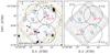 |
Fig. 1. Footprints of ALMA observations toward the MUDF. Left panel: The background shows the HST/WFC3 F140W image, and the gray lines show the PB response of the ALMA band 6 mosaic at 30% and 50% (solid and dashed lines, respectively). The orange line indicates the region observed by VLT/MUSE with >3 hours of exposure time. Red diamonds indicate the MUDF quasar pair. The blue squares with labels indicate the high-fidelity ALMA-selected sources extracted from the 1.2 mm continuum image. The dot-dashed black circles show the ALMA pointings of the band 3 spectral scans toward three individual sources (P.C1, P.C3, and P.C4). The diameter of the circles indicates the HPBW at 101 GHz. Right panel: ALMA band 6 continuum observations. The synthesized beam size is shown in the bottom right corner. |
The ALMA band 3 observations consist of three single-pointing spectral scans centered on three sources revealed in the band 6 mosaic (see, Fig. 1) to target their CO(3–2) line (rest-frame frequency νrest = 461.041 GHz) in the redshift range z≃2−3. The frequency setups were tuned based on the photometric redshift probability distributions (pointing to the redshift range 1.8≲z≲2.8) obtained from multiwavelength photometry available for galaxies in the MUDF (see, Revalski et al. 2023) using the EAZY code (Brammer et al. 2008). Observations were carried out in FDM employing five frequency tunings with two adjacent 1.875 GHz-wide SPWs per sideband designed to cover the spectral range 86.25−115.80 GHz contiguously. The total effective bandwidth is 29.55 GHz. Each frequency tuning was observed in two EBs, and executed between January 18th and March 4th 2024, employing 40 to 45 12-m antennas with baselines ranging in 15.1−483.9 m and a mean PWV = 2.7−7.1 mm. The uv coverage of these observations yields a naturally weighted synthesized beam size of  at the reference frequency of 101 GHz. The total on-source observing time was 8.1 h. Data were acquired with a native spectral resolution of 1.95 MHz, corresponding to ≃5.8 km s−1 at 101 GHz. The sensitivity achieved in the final dataset varies along with frequency due to the variation in atmospheric absorption and weather conditions across the EBs (Fig. 2) and has a median value of 0.20 mJy beam−1 over 33.7 MHz, or ≃100 km s−1 at 101 GHz. Fig. 1 shows the ALMA band 6 continuum cleaned mosaic as well as contours of the primary beam (PB) response. In Fig. 2, we show the spectral coverage of the acquired band 3 spectral scans and the sensitivity variation along the frequency range.
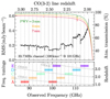 |
Fig. 2. Sensitivity (RMS) of the ALMA band 3 spectral scans across the covered frequency range. Top panel: The colored curves and the right axis report the atmospheric transmission from the ALMA site at different levels of PWV obtained using plotAtmosphere task in the CASA analysisUtils package (Hunter et al. 2023b). The top axis reports the expected redshift of the CO(3–2) line. Bottom panel: Disposition of SPWs in the four frequency tunings. Vertical dotted lines indicate the edges of the SPWs. The maximum sensitivity is achieved within z≈2.35−2.5 where two SPWs in different frequency tunings overlap. The right axis reports the redshift of the various CO transitions (dash-dotted lines) covered by the spectral scan within z≃1−4. |
2.2. Data calibration and imaging
We calibrated the data using the Common Astronomy Software Application (CASA; McMullin et al. 2007; Hunter et al. 2023a) by running the calibration pipeline scriptForPI provided with the raw measurement set using the CASA pipeline versions 6.2.1 and 6.5.4 for band 6 and 3 data, respectively. No self-calibration was performed on the datasets. We imaged band 6 visibilities by using the CASA task tclean. We first obtained a “dirty” continuum image by performing the Fourier transform of the visibilities (niter = 0) using the multi-frequency synthesis mode (specmode = “mfs”) and adopting a natural weighting scheme to maximize the sensitivity per beam. In this procedure, we set “mosaic” as the gridding convolution function and put the phase center at the coordinates ICRS 21:42:24.4658 −44:19:53.007. We used a pixel scale of  to achieve the Nyquist sampling of the longest baselines. Similarly, we obtained “dirty” band 6 data cubes of the LSB and USB with 25 km s−1 channel width. Additionally, in order to improve the surface brightness sensitivity for faint extended emission, we created a continuum image by applying a Gaussian taper in the uv plane with FWHMuv = 90 kλ and setting the pixel size to
  , yielding a synthesized beam FWHM of
  . The “dirty” data preserve the intrinsic properties of the noise, and we used that to perform a blind search of continuum and line emitters in the field (see Sect. 4). We finally obtained “cleaned” continuum images and cubes by applying the cleaning algorithm down to 2σ, placing circular masks of
  diameter around sources extracted with S/N>5.
We imaged the ALMA band 3 pointings by obtaining “dirty” cubes of the combined dataset, including all the SPWs using tclean with niter = 0 and the “natural” weighting scheme of the visibilities. We set the pixel scale at  and the channel width at 100 km s−1 at the reference frequency of 101 GHz, which is expected to maximize the S/N per channel while resolving the line profile. In such datasets, sources appear faint and spatially unresolved and no bright continuum emitters are found in the cubes. For these reasons, the cleaning of cubes is not required.
3. Ancillary multi-wavelength observations
In this study, we use the catalog of MUDF galaxies from Revalski et al. (2023), which provides deep photometry and high-confidence redshifts constrained with HST and MUSE spectroscopy, to associate optical counterparts to the sources identified by ALMA. This field benefits from extremely deep MUSE observations (ESO PID 1100.A-0528, PI: M. Fumagalli) with an integration time of ≈142 hours in wide field mode and with extended wavelength coverage (4600−9350 Å, and spectral resolution R≈2000−4000). We refer to Fossati et al. (2019a) for detailed descriptions of the survey design and the data reduction.
The MUDF survey is specifically designed to study the connection between gas and galaxies across cosmic time and thus also includes high-resolution (R≈40 000) spectra of the two quasars (QSO-SE and QSO-NW with r-band magnitude 17.9 and 20.5, respectively) to probe the IGM and CGM in absorption (see, Beckett et al. 2024). The quasar spectra were obtained using the Ultraviolet and Visual Echelle Spectrograph (UVES, Dekker et al. 2000) at the VLT (PIDs: 65.O-0299, 68.A-0216, 69.A-0204, and 102.A-0194, PI: V. D’Odorico) and cover the wavelength range 4100−9000 Å with a S/N per pixel of ≈25 and ≈10 for the bright and faint quasar, respectively.
In HST Cycle 26, we also collected 90 orbits of WFC3/F140W imaging and WFC3/IR G141 grism spectroscopy (PID 15637, PI: M. Rafelski & M. Fumagalli), providing a deep and extensive sampling of the galaxy spectral energy distributions (SEDs) from UV to NIR wavelengths (see, Revalski et al. 2024). Custom calibration of HST observations is described by Revalski et al. (2023) together with a complete list of additional optical and near-UV (NUV) photometry1.
3.1. Catalog of HST-selected galaxies
Galaxies detected in the deep WFC3/F140W image are included in a catalog that is 50% complete at 27.6 mag and covers the entire area observed with MUSE, as described by Revalski et al. (2023). To all the detected galaxies, a spectroscopic redshift is assigned together with a quality flag (see Table 5 in Revalski et al. 2023), depending on the presence of high S/N lines in their spectra. The spectral fitting process used to identify and fit emission lines across a wide range of wavelengths, from UV to NIR, is detailed in Revalski et al. (2024). A high-quality redshift (redshift quality flag ≥3) was assigned to 25% of the sources with spectral coverage. The physical properties of these galaxies, such as stellar mass (M★) and star formation rate (SFR), are obtained by fitting the multiwavelength photometry and the MUSE spectra simultaneously, as described in Fossati et al. (2018, see, also, Revalski et al. 2024), to which we refer for full details about the method. Finally, we distinguished between isolated galaxies and those residing in groups. To this end, we applied a friends-of-friends algorithm to identify galaxies belonging to a group as all the sources that are not isolated within ±500 km s−1 along the line of sight (see, e.g., Fossati et al. 2019a, for a similar approach). Overall, we found that ≈86% of the galaxies reside in 23 different groups across the redshift range z = 1−3, with five groups with more than five galaxies, and two with more than 15 members.
3.2. Catalog of quasar absorbers
The detailed procedure used to identify the absorption line systems in the spectra of the two quasars, as well as the complete list of the transitions and their properties, is illustrated in Table 1 of Beckett et al. (2024), and is only briefly summarized below. The spectra are normalized by fitting a cubic spline to the continuum redward to the Lyα emission of the quasars by using the ESPRESSO data analysis software (Cupani et al. 2016). The spectra are then visually inspected to identify absorption line systems such as Mg I, Mg II, Fe II, Al II, Al III, C IV and Si IV. All these lines are then fitted using the Bayesian code Monte Carlo Absorption Line Fitter (MC-ALF, Longobardi et al. 2023) and decomposed into the minimum number of Voigt profiles required to reproduce the observed flux. The Doppler parameter, column density, and redshift of each Voigt component are the free parameters of the fit. Additional filler components account for blends with absorption features arising from different ions at different redshifts. We finally assign the redshift of the component with the largest column density to each absorber. The resulting sample includes 22 absorption systems in the QSO-SE sightline, and nine systems in the QSO-NW sightline. Only one absorption system is detected in both the sightlines at z≈0.88 (see, Table 1 in Beckett et al. 2024). Multiple ions are often detected at the redshift of each system.
4. Extraction and characterization of ALMA sources
We performed a source search in the “dirty” ALMA band 6 continuum mosaic image using the Python-based code LINESEEKER2. The complete details of the code and performance are described in González-López et al. (2017, 2019). Here, we summarize the basic characteristics and operation of the algorithm.
LINESEEKER has been designed to perform a blind search of line emitters in large data cubes from (sub)millimeter surveys such as the ALMA Spectroscopic Survey in the Hubble Ultra Deep Field (ASPECS; see, e.g., Decarli et al. 2019; González-López et al. 2019, 2020), but can be equivalently employed to search for sources in 2D continuum images. The code searches for the line emitter in the cube by adopting a matched filter approach. LINESEEKER convolves the data cube along the spectral axis with a Gaussian kernel with a range of input widths set based on a typical linewidth. For each convolution iteration, the code finds all the voxels above a given S/N threshold. The noise is estimated in the convolved cube through 5σ-clipped statistics, and the signal is measured from the peak flux density per beam. The sources are extracted by grouping connected voxels using the Density-Based Spatial Clustering of Application with Noise algorithm (DBSCAN; Ester et al. 1996)3. Then, the final list of sources is drawn by cross-matching the source catalogs obtained from different convolution kernels and selecting the maximum S/N. For each identified candidate, LINESEEKER estimates the probability of false positive detection by performing the source search on the negative cube. Since any negative peak in a (sub)millimeter extragalactic survey is expected to be result of noise, the ratio between positive and negative detection distributions is used to estimate the fidelity (or reliability) of source candidates as a function of S/N as
where Nneg and Npos are the number of negative and positive detections at a given S/N. The cumulative distribution of negative detections is then modeled assuming Gaussian-distributed noise by using a function of the form  , where erf is the error function, and N, σ are free parameters. The best-fit model is finally used to estimate F(S/N) for all positive source candidates. The fidelity uncertainties are estimated using Poisson statistics. The search of continuum sources in 2D images can be performed similarly with LINESEEKER by skipping the convolution steps.
4.1. Continuum-selected sources in the 1.2-mm image
We selected source candidates in the ALMA band 6 mosaic by running LINESEEKER on the untapered “dirty” continuum image, excluding the region below 50% of the maximum PB response, where the low telescope sensitivity increases the probability of selecting spurious sources. The “dirty” data are preferred over the “cleaned” ones, since the former preserves the intrinsic properties of the noise. Furthermore, we input the “dirty” image into LINESEEKER without correcting for the PB response, thus preserving the spatial homogeneity of the noise across the field-of-view (FoV). With LINESEEKER we extracted all the detections above S/N>3 and selected the source candidates with F≥90%, corresponding to S/N≥5.0. We recovered a total of seven 1.2-mm continuum-selected candidates (labeled C1 to C7), including the host galaxy of the QSO-SE (C2). We report the location of these sources in Fig. 1 and their characteristics in Table 1. We performed similar search on the tapered band 6 continuum image, which is more sensitive to faint extended emission, and found consistent result.
ALMA 1.2-mm continuum-selected sources.
To further investigate the reliability of faint candidates, we complemented the search for continuum sources by cross-matching the catalog of galaxies detected in the HST/WFC3 F140W image (see Sect. 3.1) with the sources selected by LINESEEKER with fidelity values within 20%≤F<90%. To this end, we search for HST counterparts around the sky position of ALMA continuum sources within a separation limit of  , comparable to the beam size of the 1.2-mm continuum untapered image, and found no associations. For the goal of this study, we therefore include in our fiducial sample of ALMA continuum sources only the high-fidelity candidates selected as previously described. For all of these sources, we found associations in the HST catalog as described in Sect 4.4.
We evaluated the completeness of our ALMA band 6 survey by injecting artificial point-like sources at random locations in the untapered dirty 1.2-mm continuum image. Then, we computed the rate of recovered sources by running LINESEEKER and searching for candidates with F≥90% encompassed within  from the injected position, corresponding to half of the beam major axis. We repeated the simulation by injecting 20 sources simultaneously into the image and repeating this procedure for different values of flux density in the range [2, 10]×RMS. We finally iterated the entire simulation 30 times to achieve good statistics. As a result, we find that our source search is complete to ≈90% at S/N≈7.5. During the simulation, we also evaluated the effect of flux boosting (see, e.g., Hogg & Turner 1998; Scott et al. 2002; Coppin et al. 2006) on the recovered sources, and we determined that it is negligible at S/N≳5. Thus, we do not correct the measured fluxes of our source sample for this effect.
4.2. Line emitters in band 6 data cubes
The band 6 data cubes cover multiple molecular and atomic lines which enter the LSB and USB at different redshifts. In particular, for z<3.5 the carbon monoxide CO transitions are covered by our frequency setup from the CO(3–2) at z≃0.45 in the USB, to the CO(9–8) at z≃3.344, while the fine-structure lines of the atomic carbon [CI]609, 369 μm are observable from z≈0.9 up to 2.38.
To complete the source search in the field, we employed LINESEEKER to detect line emitters in the cubes blindly. Similarly to the search for continuum emitters (see Sect. 4.1), we restricted the source extraction to the survey area with PB response ≥50%, and we run the line-search algorithm on both LSB and USB cubes using a Gaussian kernel with width ranging from 1 to 18 channels, which is adequate to match the typical linewidths of FWHM∼50−1000 km s−1 observed in high-redshift galaxies (see, e.g., Birkin et al. 2021). We extracted all line-emitting candidates with S/N≥3.0 and then selected those with F≥90%. This resulted in one line emitter, which corresponds to the C6 source, which we already identified through its continuum at 1.2 mm (see Table 1). This source has a robust spectroscopic redshift of z = 1.05413 measured with the MUSE data (see Sect. 4.4) that allowed us to identify the line as [CI]609 μm. We measured the line flux and width by fitting the spectrum extracted from the source peak pixel (see, Sect. 4.5), and obtained ![$ F_{{\rm [CI]}609\,\mathrm{\mu} {\rm m}} = 0.36^{+0.10}_{-0.09}\,{\rm Jy\,beam^{-1}\,km\,s^{-1}} $](/articles/aa/full_html/2025/04/aa52462-24/aa52462-24-eq15.gif) ,
,  , respectively (see Appendix B). The source redshift we estimated with this line is consistent with the one measured from the MUSE spectrum. The visual inspection of ALMA band 6 spectra at the location of all the 1.2-mm continuum-selected sources did not reveal additional emission lines, consistently with the spectroscopic redshift measurements of the sources.
Finally, we complemented our line search by cross-matching the HST catalog of galaxies with the source catalog of line-emitting candidates delivered by LINESEEKER following the same approach described in Sect. 4.1. This procedure did not reveal additional line emitters.
4.3. Source detection in band 3 spectral scans
We analyzed ALMA band 3 spectral scans targeting sources C1, C3, and C4. We inspected the spectra at the center of the pointing around the nominal locations of their continuum detections revealed at 1.2 mm in the ALMA mosaic (see Table 1). The CO(3–2) line, which is identified based on the posterior distributions of the source photometric redshift5, is detected in all three sources, which appear spatially unresolved given the low angular resolution of these ALMA observations (see Sect. 2).
We ran LINESEEKER on band 3 “dirty” cubes and continuum images similarly to what described in Sects. 4.1 and 4.2 for band 6 data. The search for additional line emitters within the cubes, including cross-matching between low-fidelity ALMA candidates with HST/MUSE-selected galaxies, resulted in the detection of the CO(4–3) line of the C2 (QSO-SE) which is redshifted in the ALMA band 3 at z≃3.2267. The analysis of this detection is reported in Appendix B. Additionally, we performed visual inspection of the band 3 spectra at the location of secure continuum sources selected in the ALMA band 6 mosaic, and found no evident emission lines. Finally, in the 3-mm continuum images we did not find neither high-fidelity source candidates, nor HST counterparts associated to the low-fidelity ones.
4.4. HST counterparts of ALMA continuum sources
In Fig. 3, we show postage stamps of the seven ALMA continuum-selected sources and their NIR and optical/NUV counterparts in the field. As also described in Sect. 4.1, we cross-matched all the sources detected in the continuum at 1.2 mm with ALMA with the catalog of HST-selected galaxies. Within a projected separation of  in the sky, we found an unambiguous counterpart for all ALMA detections, except for C5. By visually inspecting the HST/WFC3 F140W image of this source, we found that the peak of the ALMA continuum appears to correspond to a faint and compact source located southeast relative to an extended disk-like object. Interestingly, the 1.2-mm continuum emission seems to be spatially associated with diffuse emission revealed by HST around the extended galaxy, which suggests irregular morphology, possibly due to the interaction with the nearby compact source. Alternatively, the observed millimeter emission of C5 might trace a very dusty galaxy with differential obscuration along the line of sight, resulting in an apparent offset relative to the rest-frame optical/UV detections (e.g., Chen et al. 2017). An additional interpretation sees the ALMA detection associated with a source lensed by the closely separated disk galaxy detected by HST (e.g. Vieira et al. 2013). However, given the limited S/N of the ALMA data and the lack of secure spectroscopic redshift measurements, we cannot confidently assess the nature of this emission. The angular resolution of MUSE observations is insufficient for adequately deblending the spectra of these two closely spaced sources (see, Fig. 3). By inspecting the MUSE spectrum extracted at the location of the galaxies, we assigned to both the sources a low-quality redshift estimate of z≈2.47 on the basis of only the tentative detection of C IV λλ1548, 1550 absorption line feature. At this redshift, the CO(3–2) line is redshifted in ALMA band 3. However, despite C5 is in the FoV of the C1 spectral scan, we did not detect this line. Future deep spectroscopic observations using, for example, JWST, are needed to shed light on the characteristics of this system.
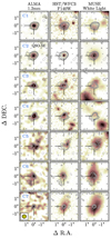 |
Fig. 3. 5″×5″ postage stamps of NIR and optical/NUV counterparts of ALMA 1.2-mm continuum-selected sources in the MUDF. From left to right: 1.2-mm continuum map from ALMA band 6, HST/WFC3 F140W (central observed wavelength 1.4 μm), MUSE white light image (central observed wavelength 655 nm). The solid contours show the [2, 3, 2n]×RMS (with n≥2) levels of the ALMA continuum. The yellow ellipse at the corner of the bottom left panel shows the synthesized ALMA beam. |
A high-quality spectroscopic redshift is constrained from the MUSE spectra for C2, C6, and C7. The remaining ones (i.e., C1, C3, and C4), which are also the faintest in the F140W filter among the counterparts (see, Table 1), do not have a secure redshift measurement from MUSE or HST grism spectra. The redshifts of the latter, are accurately measured from the CO(3–2) lines detected in the band 3 spectral scans as previously described in Sect. 4.3.
4.5. Source fluxes and luminosities
All seven ALMA-selected sources detected in the continuum at 1.2 mm appear, at best, marginally resolved. To maximize the recovered signal, we estimated their flux density in the ∼2″ tapered image through a single-pixel measurement of the continuum source flux peak that we then rescaled for the PB response at the corresponding location. We then applied the same PB rescaling to the RMS (in mJy beam−1) measured on the 1.2-mm continuum image to estimate the 1σ uncertainty on F1.2 mm. We report these quantities in Table 1.
We measured the CO(3–2) line flux of C1, C3, and C4 detected in the band 3 cubes by fitting the spectra extracted from the source peak employing a single Gaussian plus a constant to model the line and the continuum. We then estimated the best-fit model parameters and uncertainties from the posterior probability distributions obtained through the Python Markov chain Monte Carlo (MCMC) ensemble sampler emcee package (Foreman-Mackey et al. 2013), assuming box-like priors based on a visual inspection of the data. We finally derived the line luminosities as (see, e.g., Solomon et al. 1997):
![$$ L_{\rm CO} [L_{\odot }] = 1.04\times 10^{-3}\,S\Delta {v}\,\nu _{\rm obs}\,D_{\rm L}^2, $$](/articles/aa/full_html/2025/04/aa52462-24/aa52462-24-eq18.gif)
![$$ L^{\prime }_{\rm CO} [{\rm K\,km\,s^{-1}\,pc^2}] = 3.25\times 10^7\,S\Delta {v}\,\frac {D_{\rm L}^2}{(1+z)^3\,\nu _{\rm obs}^2}, $$](/articles/aa/full_html/2025/04/aa52462-24/aa52462-24-eq19.gif)
where SΔv is the velocity-integrated line flux in Jy km s−1, νobs is the observed central frequency of the line in GHz, z is the source redshift measured from the centroid of the CO line, and DL is the luminosity distance in Mpc. The relation between Eqs. (2) and (3) is  , where νrest is the line rest frequency in GHz. In Fig. 4, we show the spectra and the best-fit models and report the line measurements in Table 2.
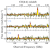 |
Fig. 4. Spectra extracted from ALMA band 3 spectral scans toward 1.2-mm continuum-selected sources C1, C3 and C4 (from the top to the bottom panel). Data and the best-fit model are shown in yellow and red, respectively. The ±1σ RMS noise range of the data is indicated by the gray shaded area. The top scale reports the expected CO(3–2) line redshift depending on the observed frequency. |
ALMA CO(3–2) line emitters.
5. Linking galaxies to absorbers in multiwavelength datasets
Absorption studies toward background quasars typically target galaxies in their rest-frame optical/UV. So far, (sub)millimeter studies (e.g., with ALMA) have focused on specific classes of absorbers, such as high-column-density DLAs (NH I≥1020.3 cm−2; see, e.g., Neeleman et al. 2017; Kanekar et al. 2018; Kaur et al. 2022a, b). However, little is known about the contribution of dusty and gas-rich galaxies to the cosmic metal enrichment across different epochs of the Universe from untargeted observations (Dudzevičiūtė et al. 2021). In this work, we capitalize on our blind ALMA survey to study the association between cosmic gas traced by quasar absorption systems in the MUDF, and galaxies detected at millimeter wavelengths in their dust continuum.
5.1. Gas-galaxy association rate
With accurate redshift measurements (Δv≲60 km s−1) of our ALMA-selected galaxies from either MUSE spectra or, when available, emission lines detected with ALMA (see Sects. 4.4, 4.5, and Appendix B), we matched these galaxies with the absorbers in velocity space in either of the quasar sightlines (see, Sect. 3.2). Following the approach typically adopted in the literature for optical studies (see, e.g., Dutta et al. 2021; Schroetter et al. 2021; Galbiati et al. 2023; Beckett et al. 2024), we link the absorbing gas with galaxies by searching for association within  with respect to the absorbers. We report our results in Fig. 5. We found that 100% of our ALMA-selected galaxies – for which robust spectroscopic redshifts are available – are unambiguously associated with metal absorbers. This detection rate decreases to ≥85% when considering the uncertainties related to source C5 (see Sect. 4.4 for details). Indeed, if we adopt the tentative redshift of C5 measured from the low-quality MUSE spectrum (z≈2.47), we find no connected absorbers for this source. For comparison, we found that only ≈25% of all spectroscopically confirmed HST-selected galaxies with log M★/M⊙≥8 are associated with absorbers, increasing to ≈45% considering galaxies with log M★/M⊙≥10. Therefore, the association rate for galaxies selected in their rest-frame optical/UV is much lower than that observed for on-average more massive galaxies selected with ALMA in their dust continuum (see, Sect 5.2).
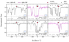 |
Fig. 5. Connection between ALMA-selected galaxies and absorption systems in the spectra of the QSO-SE (black) and -NW (purple). The line-of-sight separations are centered on the redshift of the ALMA-selected galaxies. The vertical gray band indicates the velocity at which the optical depth of the absorption is 50% of the total (τ50). The transitions shown (C IV λ1548, Al II λ1670, and Mg II λ2796) are limited to the strongest lines among the multiple metals associated to each galaxy. Galaxies selected with ALMA are indicated by red diamonds with errorbars reporting uncertainties on their redshift measurements. The panels are ordered (from the top left to the bottom right panel) for increasing sky-projected separation (R) from the QSO sightline along which the absorption is detected. HST-selected galaxies linked to the same absorbers are shown with black triangles. The number of galaxies (Ngal) associated to each group (see, Sect. 5.3) is also reported. |
Interestingly, we note that three out of the six sources (i.e., C1, C3, and C4) for which we find a robust association to absorbers would have been missed if only relying on MUSE and HST identifications. Indeed, such sources are the faintest among the NIR/optical counterparts (see Table 1) and lie in the MUSE redshift desert. This implies that studies limited to optical wavelengths may miss a significant fraction of the galaxy population around metal absorbers, as also highlighted in previous works (see, e.g., Neeleman et al. 2017, 2018, 2019; Fynbo et al. 2018; Galbiati et al. 2024). Moreover, as the case of C4 exemplifies, ALMA is critical to identify the only galaxy we can associate with the QSO-NW absorber at z = 2.368, as no other galaxies were previously known at this redshift through MUSE and HST (see, Fig. 5).
We evaluated the number density of our ALMA-selected galaxies by computing the completeness-corrected 1.2-mm number counts and found that these are consistent with that derived in blank field from ASPECS (González-López et al. 2020). In light of the above considerations, we conclude that, since obscured massive galaxies selected with ALMA have sufficient number density to be relevant in absorption line studies, blind (sub)millimeter follow-ups of optical/NIR surveys are thus essential in providing the most complete view of the galaxy population residing around absorbers.
5.2. Properties of the ALMA galaxies around absorbers
In Fig. 6, we compare the stellar mass and SFR of the dusty galaxies detected with ALMA (see Appendix A for full details) to the rest of the optical/UV-selected galaxy population in the MUDF and the sample of submillimeter galaxies (SMG) from Dudzevičiūtė et al. (2020) at z∼1−2.5. The ALMA sources lie at the high-mass end of the stellar mass function at those redshifts and are among the most massive members of the groups in which they reside (see Sect. 5.3). On the other hand, our ALMA galaxies appear to be less massive, but within in the scatter of the population of SMGs at similar epochs, lying on the asymptotic part of the main sequence at z≃1−2 (see, Popesso et al. 2023), although close to the starburst region.
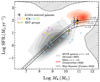 |
Fig. 6. Star formation rate-stellar mass diagram of galaxies detected in the MUDF. The gray density contours show the distribution of all galaxies selected with HST in the rest-frame optical/UV at z∼1−2. The marginalized distributions of M★ and SFR are also shown on the top and right axis, respectively. The red density contours report the sample of SMG with photometric redshift within 1≤z≤2.5 from Dudzevičiūtė et al. (2020). The ALMA-selected galaxies with properties derived from SED modeling are reported with diamonds. Colored triangles mark the HST-selected group galaxies associated with the same absorption system of each ALMA-selected galaxy. The star-forming main sequence at z∼1−2 from Popesso et al. (2023) is also shown. |
Using our measurements of the galaxy flux density at 1.2 mm on the Rayleigh-Jeans tail of the dust SED, we provide rough estimates of the dust masses (Mdust) of ALMA continuum-selected galaxies (excluding C5 for which we do not have reliable redshift measurement, and C2 that is the QSO-SE). By following a typical approach adopted in (sub)millimeter studies of high-redshift galaxies (e.g. Casey 2012; Riechers et al. 2013; Faisst et al. 2020), we employ a single modified black-body emission assuming a characteristic dust temperature of Tdust = 32 K, and emissivity index β = 1.8 typical of SMGs (see Dudzevičiūtė et al. 2020), and we find values in the range log (Mdust/M⊙)≃8.0−8.6. Using the same assumptions, we find a lower value of log (Mdust/M⊙)≃7.8 for C7, which appears to be more similar to typical main-sequence galaxies. By integrating the black-body models we computed the IR luminosities and converted them to SFRIR using the calibration from Murphy et al. (2011), and find values in the range log (SFRIR/M⊙ yr−1)≃1.6−2.4, comparable to those we derived from galaxy SED modeling (see Table A.1.).
Results from SED fitting of the ALMA-selected galaxies.
From the CO(3–2) emission line in C1, C3, and C4, and the [CI]609 μm line detected in C6 (see, Sect. 4.2), we derive estimates of galaxy molecular gas fractions. For C1, C3, and C4 we adopt a CO(3–2)-to-CO(1–0) conversion factor of r31 = 0.80±0.14 from Boogaard et al. (2020) and a range of αCO. At the lower end, we use a value of 0.8 M⊙/(K km s−1 pc2), typical of SMGs and quasar hosts (see, e.g., Downes & Solomon 1998). At the upper end, we adopt 4.3 M⊙/(K km s−1 pc2) as measured in giant molecular clouds in the Milky Way (see, e.g., Bolatto et al. 2013; Carilli & Walter 2013). For C6, we first derive atomic carbon mass from Equation (2) in Weiß et al. (2005) and we convert it to molecular gas mass by assuming a C-to-H2 abundance ratio of ![$ X{\rm [CI]}/X{\rm [H_2]}=M_{\rm CI}/(6\,M_{\rm H_2})=(8.4\pm 3.5)\times 10^{-5} $](/articles/aa/full_html/2025/04/aa52462-24/aa52462-24-eq38.gif) , as derived by Walter et al. (2011) for a sample of z∼2−3 FIR-bright sources. By employing such recipes, we find
, as derived by Walter et al. (2011) for a sample of z∼2−3 FIR-bright sources. By employing such recipes, we find  ,
,  ,
,  , and
, and  for C1, C3, C4, and C6 respectively. These values are scattered in the typical range observed in both main-sequence galaxies and ULIRGs/SMGs at z≳1 (see, e.g., Tacconi et al. 2018; Birkin et al. 2021). Interestingly, we note that C1 and C6 exhibit high values of the gas fraction and also live in rich groups (see, Sect. 5.3). This fact might suggest that efficient gas accretion is in place in these structures.
5.3. The link between the large-scale galaxy environment and the absorbing gas
In Sect. 3.1, we found that many HST-selected sources do not live in isolation but are associated with galaxy groups instead. In Fig. 7, we show that four (out of six) of our dusty galaxies (i.e., C1, C3, C6, and C7) detected with ALMA actually live in such overdense regions6. This is also evident from Fig. 5, in which multiple galaxies selected in HST are found to be associated with the same absorbers as those identified around ALMA galaxies. The high association rate between galaxies in groups and absorbers has also been found in previous works (see, e.g., Nielsen et al. 2018; Dutta et al. 2020; Hamanowicz et al. 2020; Lofthouse et al. 2023; Qu et al. 2023), suggesting that the large-scale environment plays a significant role in shaping the absorption properties. Indeed, these absorbers exhibit multiple components and are observed to be strong, showing typical rest-frame equivalent widths of EWCIV≳0.3 Å, EWMgII≳1 Å, and with complex kinematics. In particular, we note that dust-mass-selected sources living in groups of more than two galaxies (i.e., C1, C3, and C6) are associated with absorbers exhibiting high column density of NAlII, MgII≳1016 cm−2, while C4, and C7 show significantly lower values of NCIV, MgII≃1013−1014 cm−2. Other works which studied quasar absorption around galaxy groups at different redshifts reported similar evidence (see, e.g., Lan et al. 2014; Fossati et al. 2019a; Dutta et al. 2021; Nelson et al. 2021; Galbiati et al. 2023, 2024).
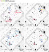 |
Fig. 7. Groups of galaxies around ALMA sources (blue squares). The colored triangles indicate the HST-selected galaxies belonging to the same group found around the redshift of ALMA sources (bottom left corner). The two quasars in the MUDF are labeled with red diamonds, the black arrow indicates the QSO sightline in which absorption at the redshift of each group is detected. The black crosses mark the projected location of the galaxy stellar mass-weighted barycenter of the groups. The gray solid and dashed lines report the PB response at 0.3 and 0.5, respectively, of the ALMA band 6 mosaic. |
We now turn to investigate the 3D separation between galaxies and the associated gas structures. In Fig. 8 we report |Δv(τ50)|−Δv90/2 against the impact parameters of galaxies associated to absorbers normalized by their virial radius7 (Rvir). Here, Δv(τ50) is the galaxy systemic velocity shift from the absorption line center, which we defined as the wavelength corresponding to 50% of the total optical depth (τ50) of the absorption. Due to the complex line profiles, we employed Δv90 as a proxy of the linewidth, which we parametrized as the velocity interval containing 90% of the total optical depth. In this phase-space diagram, a significant contribution from the gas retained in the “inner” CGM is expected to arise from galaxies located within |Δv(τ50)|−Δv90/2 < 0 km s−1, and R/Rvir<1. By looking at all the galaxies belonging to individual groups, different cases can be identified. The dusty galaxies selected with ALMA are more aligned in velocity space with the center of absorption features than the other connected galaxies. In particular, C1 and C6, which are part of rich groups, have velocities consistent with τ50 of the associated absorbers (see, Fig. 5). Similarly, despite living in less overdense regions, we find that the remaining ALMA-identified galaxies (i.e., C3, C4, and C7) lie within ±50 km s−1 from the edge of the connected absorption line profile (i.e., |Δv(τ50)|−Δv90/2 ≈ 0 km s−1) and within 100 km s−1 from τ50. This fact, in combination with their large mass (see, Sect. 5.2), suggests that these galaxies sit close to the center of the gravitational potential well of the large-scale structures that host them. However, the impact parameters of the ALMA galaxies are typically large, of the order of ∼200−400 kpc or R/Rvir up to ∼4 (see also Fig. 7). Therefore, our findings suggest that the absorbing gas is not often located in the inner CGM of the massive dusty galaxies. Rather, they act as signposts of the large scale structures that host the absorbers. Within these structures, absorption lines can arise from diffuse gas not bound to the CGM (as seen, e.g., in Galbiati et al. 2023) or from the CGM of other galaxies at close impact parameter from the quasar. Fig. 8 confirms these various scenarios, with only some examples of galaxies lying in the |Δv(τ50)|−Δv90/2 < 0 km s−1, R/Rvir≲1 region. Finally, complementary to this picture, we note that in the cases of systems clustered in small volumes (e.g., C3 group), hydrodynamical and gravitational interactions may play an important role in shaping the properties of the surrounding gas (see, e.g, Gunn & Gott 1972; Merritt 1983; Boselli & Gavazzi 2006; Klitsch et al. 2019).
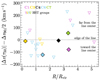 |
Fig. 8. Phase-space diagram of the galaxies identified with ALMA and of the other group members associated with quasar absorbers. The vertical axis reports the difference between the velocity shift from the absorption line center, measured from the τ50 wavelength (Δv(τ50)), and half of the Δv90 of the absorption profile. Negative values indicate that the galaxy systemic is near to the center of the absorption profile, while positive ones correspond to galaxies at the redshift of which no absorption is detected. The horizontal axis shows the galaxy impact parameters normalized by their virial radius (Rvir). The markers are color-coded as in Fig. 6. |
In light of the aforementioned considerations, we test the hypothesis that the observed absorption profiles associated with groups could potentially arise from the superposition of the halos of multiple galaxies located around the massive sources identified with ALMA (see, e.g., Bordoloi et al. 2011; Nielsen et al. 2018; Dutta et al. 2020). One might expect the strength of the absorption to correlate with the projected galaxy surface density (see, e.g., Galbiati et al. 2024). We centered on the sky position and redshift of ALMA galaxies C1, C3, C6 and C7, and count the number of HST-selected sources within a velocity window of |Δv| ≤ 250 km s−1 (chosen based on the broadest absorption system, see Fig. 5), and encompassed radius corresponding to the impact parameter from the QSO. We then divide the number of galaxies by the projected area corrected for the coverage of the MUSE FoV. In Fig. 9, we report such galaxy surface density against the EW of the associated absorbers8. As a result, we find a hint of positive correlation9, which is consistent with the scenario proposed above. In order to show the potential correlation, we fit the data with a linear model by employing the Python MCMC ensemble sampler emcee package (Foreman-Mackey et al. 2013) adopting a Poisson maximum likelihood estimator and flat priors on the free parameters. In Fig. 9, we report the best fit and 1σ confidence interval. However, we note that our analysis relies on a handful of sources and therefore is limited by the low statistics. In addition, as discussed above (see, Fig. 8), only a fraction of galaxies in groups seems to contribute to the observed absorption profiles with the gas retained in their halos (i.e., within Rvir). Hence, surveys designed to explore a broader range of galaxy overdensities around absorbers and to provide larger statistical samples are needed to draw more robust conclusions.
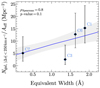 |
Fig. 9. Galaxy surface density in groups as a function of EW of the associated absorbers (Mg II for C1, C6, and C7, and Al II for C3, respectively). Number density is computed by counting the number of galaxies (Ngal), and dividing for the effective area (Aeff) as described in Sect. 5.3. The associated uncertainties are obtained from Poisson statistics for low number counts (Gehrels 1986). The blue solid line and gray shaded area are the best fit linear model (Ngal/Aeff=a×(EW/Å)+b Mpc−2, with a = 4±2, b = 4±3) and 1σ confidence interval, respectively. The Spearman's rank correlation coefficient and the corresponding p-value are also reported. |
6. Summary and conclusions
In this work, we presented an ALMA blind dust continuum and molecular gas survey around the sightlines of the z≈3.22 quasar pair in the MUDF. By combining our (sub)millimeter observations with available multiwavelength data from NIR to UV, we investigated the role of the dusty galaxy population in association to the intervening gas structures revealed in absorption in the quasar spectra. Below, we summarize our main findings:
-
We identified a robust sample of seven sources detected at 1.2-mm in their dust continuum with ALMA. We determined the spectroscopic redshift of six of them from either the inspection of their MUSE spectra or via the emission lines detected in ALMA observations.
-
We found that the dust-selected galaxies and metal absorbers are associated within 500 km s−1. This implies that at least ≥85% of the dusty galaxies uncovered with ALMA are unambiguously linked to multiple absorption features arising from metal ions and observed in either of the quasar sigthlines. This association rate is significantly higher than in previous surveys at NIR–UV wavelengths.
-
By combining multiband photometry and information about dust and molecular gas gathered from our (sub)millimeter data, we investigated the nature of the ALMA-selected galaxies by performing SED modeling. As a result, most of these galaxies appear massive (M★≃1010.2−10.7 M⊙), highly star forming (SFR≃101.2−2.0 M⊙ yr−1), and exhibit high dust and molecular gas content (Mdust≃107.8−8.6 M⊙, fH2≃20−65%), resembling typical SMGs at similar redshifts.
-
We discovered that a large fraction of the spectroscopically confirmed ALMA-selected sources (≳65%) live in galaxy groups in which they are among the most massive members. While the associated absorbers show complex kinematics, the ALMA-detected galaxies are better aligned with the center of the absorption features than the other galaxies previously identified in the optical. This may suggest that these massive and dust-obscured galaxies sit close to the center of the gravitational potential well of their large-scale structures. However, the impact parameters of the ALMA galaxies are typically large, ∼200−400 kpc, indicating that absorption probed by the QSO sightlines might originate from the gas distributed within a few virial radii.
This study highlights the crucial role of (sub)millimeter surveys to obtain a complete census of the galaxy population around metal enriched cosmic gas structures revealing the presence of massive and dust-obscured galaxies. Overall, our findings suggest that massive dusty galaxies appear to be signposts of the large-scale structures that host them rather than the actual sites of the absorbing gas. Though, we caution that this emerging evidence may also be a consequence of the low number density of these galaxies. Moreover, focused surveys of SMGs at small separations from QSOs will enable investigations of the inner CGM at the interface with the ISM of dusty galaxies and will allow for a statistical assessment of our conclusions. Finally, further efforts are needed to understand which processes are responsible for distributing metals into the IGM and how different galaxy populations contribute to the metal enrichment across the cosmic time.
Acknowledgments
We thank the anonymous referee for the valuable comments and suggestions which significantly improved the manuscript. This paper uses the following ALMA data: ADS/JAO.ALMA#2021.1.00285.S, ADS/JAO.ALMA#2023.1.00461.S. ALMA is a partnership of ESO (representing its member states), NSF (USA) and NINS (Japan), together with NRC (Canada), MOST and ASIAA (Taiwan), and KASI (Republic of Korea), in cooperation with the Republic of Chile. The Joint ALMA Observatory is operated by ESO, AUI/NRAO and NAOJ. Based on observations with the NASA/ESA Hubble Space Telescope obtained from the MAST Data Archive at the Space Telescope Science Institute, which is operated by the Association of Universities for Research in Astronomy, Incorporated, under NASA contract NAS5-26555. Support for program Nos. 15637 and 15968 was provided through a grant from the STScI under NASA contract NAS5-26555. These observations are associated with program Nos. 6631, 15637, and 15968. The MUSE portion of this project has received funding from the European Research Council (ERC) under the European Union Horizon 2020 research and innovation program (grant agreement No. 757535) and by Fondazione Cariplo (grant No. 2018-2329). This project was supported by the ERC Consolidator Grant 864361 (CosmicWeb) and by Fondazione Cariplo grant no. 2018-2329, 2020-0902. IRS acknowledges support from STFC (ST/X001075/1). This research made use of Astropy (http://www.astropy.org), a community-developed core Python package for Astronomy (Astropy Collaboration 2013, 2018, 2022), NumPy (Harris et al. 2020), SciPy (Virtanen et al. 2020), Matplotlib (Hunter 2007).
The final products can be retrieved as High Level Science Products (HLSPs) at doi: 10.17909/81fp-2g44, together with the default data files at doi: 10.17909/q67p-ym16 from the Mikulski Archive for Space Telescopes (MAST). The dedicated page to the MUDF program is available at https://archive.stsci.edu/hlsp/mudf
The code is publicly available at https://github.com/jigonzal/LineSeeker. Other similar source-finding codes are available in the literature, such as FINDClumps (Walter et al. 2016) or MF3D (Pavesi et al. 2018), which differ mainly in details about the adopted spectral filter function. However, comparisons between codes have yielded very similar results (see González-López et al. 2019).
This algorithm is included within the Python package Scikit-learn (Pedregosa et al. 2011).
We derived photometric redshifts of C1, C3 and C4 from multiband photometry as detailed in Sect. 2, obtaining zphot = 2.21±0.19, 2.51±0.07, 2.44±0.17, respectively, where nominal values and uncertainties are computed from the expected value and variance of the photometric redshift posteriors.
From the total stellar mass of the groups we estimated the dark matter halo masses of the systems in which ALMA galaxies reside by employing the stellar-to-halo mass relation from Moster et al. (2010), and obtain an average halo mass of ∼1013 M⊙.
We estimated the virial radius by converting the galaxy stellar mass into dark matter halo mass following Moster et al. (2010). For a halo mass of 1012.5 M⊙, typical of z≳1 ALMA-selected galaxies (Hickox et al. 2012; Wilkinson et al. 2017; Lim et al. 2020; Stach et al. 2021), the virial radius is Rvir≈200 and 150 kpc at z = 1 and 2, respectively.
We used Mg II for C1, C6, and C7, and Al II for C3, since we have no Mg II detection for this source. These are chosen as they have similar  , where fosc is the oscillator strength, and
  is the rest-frame wavelength of the transitions. However, we caution that due to the differences in the relative abundances, at fixed EW different ions do not trace the same gas density.
The Spearman's rank correlation test (Spearman 1904) yields a degree of monotonic correlation of ρ = 0.8 with a p-value 0.1, indicating that a positive correlation is in place at 80% confidence level.
References
- Astropy Collaboration (Robitaille, T. P., et al.) 2013, A&A, 558, A33 [NASA ADS] [CrossRef] [EDP Sciences] [Google Scholar]
- Astropy Collaboration (Price-Whelan, A. M., et al.) 2018, AJ, 156, 123 [Google Scholar]
- Astropy Collaboration (Price-Whelan, A. M., et al.) 2022, ApJ, 935, 167 [NASA ADS] [CrossRef] [Google Scholar]
- Bacon, R., Accardo, M., Adjali, L., et al. 2010, SPIE Conf. Ser., 7735, 773508 [Google Scholar]
- Bacon, R., Mary, D., Garel, T., et al. 2021, A&A, 647, A107 [NASA ADS] [CrossRef] [EDP Sciences] [Google Scholar]
- Banerjee, E., Muzahid, S., Schaye, J., Johnson, S. D., & Cantalupo, S. 2023, MNRAS, 524, 5148 [NASA ADS] [CrossRef] [Google Scholar]
- Beckett, A., Rafelski, M., Revalski, M., et al. 2024, ApJ, 974, 256 [NASA ADS] [Google Scholar]
- Birkin, J. E., Weiss, A., Wardlow, J. L., et al. 2021, MNRAS, 501, 3926 [Google Scholar]
- Bolatto, A. D., Wolfire, M., & Leroy, A. K. 2013, ARA&A, 51, 207 [CrossRef] [Google Scholar]
- Boogaard, L. A., van der Werf, P., Weiss, A., et al. 2020, ApJ, 902, 109 [NASA ADS] [CrossRef] [Google Scholar]
- Bordoloi, R., Lilly, S. J., Knobel, C., et al. 2011, ApJ, 743, 10 [CrossRef] [Google Scholar]
- Borisova, E., Cantalupo, S., Lilly, S. J., et al. 2016, ApJ, 831, 39 [Google Scholar]
- Boselli, A., & Gavazzi, G. 2006, PASP, 118, 517 [Google Scholar]
- Brammer, G. B., van Dokkum, P. G., & Coppi, P. 2008, ApJ, 686, 1503 [Google Scholar]
- Bruzual, G., & Charlot, S. 2003, MNRAS, 344, 1000 [NASA ADS] [CrossRef] [Google Scholar]
- Byler, N., Dalcanton, J. J., Conroy, C., et al. 2018, ApJ, 863, 14 [NASA ADS] [CrossRef] [Google Scholar]
- Calzetti, D., Armus, L., Bohlin, R. C., et al. 2000, ApJ, 533, 682 [NASA ADS] [CrossRef] [Google Scholar]
- Cantalupo, S. 2017, Astrophys. Space Sci. Lib., 430, 195 [NASA ADS] [CrossRef] [Google Scholar]
- Carilli, C. L., & Walter, F. 2013, ARA&A, 51, 105 [NASA ADS] [CrossRef] [Google Scholar]
- Casey, C. M. 2012, MNRAS, 425, 3094 [Google Scholar]
- Chabrier, G. 2003, PASP, 115, 763 [Google Scholar]
- Chen, H. -W., Helsby, J. E., Gauthier, J. -R., et al. 2010a, ApJ, 714, 1521 [NASA ADS] [CrossRef] [Google Scholar]
- Chen, H. -W., Wild, V., Tinker, J. L., et al. 2010b, ApJ, 724, L176 [NASA ADS] [CrossRef] [Google Scholar]
- Chen, C. -C., Hodge, J. A., Smail, I., et al. 2017, ApJ, 846, 108 [Google Scholar]
- Coppin, K., Chapin, E. L., Mortier, A. M. J., et al. 2006, MNRAS, 372, 1621 [Google Scholar]
- Cupani, G., D’Odorico, V., Cristiani, S., et al. 2016, SPIE Conf. Ser., 9913, 99131T [Google Scholar]
- Dale, D. A., Helou, G., Magdis, G. E., et al. 2014, ApJ, 784, 83 [Google Scholar]
- Decarli, R., Walter, F., Gónzalez-López, J., et al. 2019, ApJ, 882, 138 [Google Scholar]
- Dekker, H., D’Odorico, S., Kaufer, A., Delabre, B., & Kotzlowski, H. 2000, SPIE Conf. Ser., 4008, 534 [Google Scholar]
- Downes, D., & Solomon, P. M. 1998, ApJ, 507, 615 [NASA ADS] [CrossRef] [Google Scholar]
- Dudzevičiūtė, U., Smail, I., Swinbank, A. M., et al. 2020, MNRAS, 494, 3828 [Google Scholar]
- Dudzevičiūtė, U., Smail, I., Swinbank, A. M., et al. 2021, MNRAS, 500, 942 [Google Scholar]
- Dutta, R., Fumagalli, M., Fossati, M., et al. 2020, MNRAS, 499, 5022 [CrossRef] [Google Scholar]
- Dutta, R., Fumagalli, M., Fossati, M., et al. 2021, MNRAS, 508, 4573 [NASA ADS] [CrossRef] [Google Scholar]
- Dutta, R., Fumagalli, M., Fossati, M., et al. 2024, A&A, 691, A236 [NASA ADS] [CrossRef] [EDP Sciences] [Google Scholar]
- Ester, M., Kriegel, H. P., Sander, J., & Xu, X. 1996, Second International Conference on Knowledge Discovery and Data Mining (KDD’96). Proceedings of a conference held August 2–4, 226 [Google Scholar]
- Faisst, A. L., Fudamoto, Y., Oesch, P. A., et al. 2020, MNRAS, 498, 4192 [NASA ADS] [CrossRef] [Google Scholar]
- Foreman-Mackey, D., Hogg, D. W., Lang, D., & Goodman, J. 2013, PASP, 125, 306 [Google Scholar]
- Fossati, M., Mendel, J. T., Boselli, A., et al. 2018, A&A, 614, A57 [NASA ADS] [CrossRef] [EDP Sciences] [Google Scholar]
- Fossati, M., Fumagalli, M., Lofthouse, E. K., et al. 2019a, MNRAS, 490, 1451 [NASA ADS] [CrossRef] [Google Scholar]
- Fossati, M., Fumagalli, M., Gavazzi, G., et al. 2019b, MNRAS, 484, 2212 [NASA ADS] [CrossRef] [Google Scholar]
- Fumagalli, M., O’Meara, J. M., & Prochaska, J. X. 2016, MNRAS, 455, 4100 [NASA ADS] [CrossRef] [Google Scholar]
- Fynbo, J. P. U., Heintz, K. E., Neeleman, M., et al. 2018, MNRAS, 479, 2126 [NASA ADS] [CrossRef] [Google Scholar]
- Galbiati, M., Fumagalli, M., Fossati, M., et al. 2023, MNRAS, 524, 3474 [NASA ADS] [CrossRef] [Google Scholar]
- Galbiati, M., Dutta, R., Fumagalli, M., Fossati, M., & Cantalupo, S. 2024, A&A, 690, A7 [NASA ADS] [CrossRef] [EDP Sciences] [Google Scholar]
- Gehrels, N. 1986, ApJ, 303, 336 [Google Scholar]
- González-López, J., Bauer, F. E., Romero-Cañizales, C., et al. 2017, A&A, 597, A41 [NASA ADS] [CrossRef] [EDP Sciences] [Google Scholar]
- González-López, J., Decarli, R., Pavesi, R., et al. 2019, ApJ, 882, 139 [Google Scholar]
- González-López, J., Novak, M., Decarli, R., et al. 2020, ApJ, 897, 91 [Google Scholar]
- Gunn, J. E., & Gott, J. R. 1972, ApJ, 176, 1 [NASA ADS] [CrossRef] [Google Scholar]
- Hamanowicz, A., Péroux, C., Zwaan, M. A., et al. 2020, MNRAS, 492, 2347 [CrossRef] [Google Scholar]
- Harris, C. R., Millman, K. J., van der Walt, S. J., et al. 2020, Nature, 585, 357 [NASA ADS] [CrossRef] [Google Scholar]
- Hennawi, J. F., & Prochaska, J. X. 2013, ApJ, 766, 58 [NASA ADS] [CrossRef] [Google Scholar]
- Hickox, R. C., Wardlow, J. L., Smail, I., et al. 2012, MNRAS, 421, 284 [NASA ADS] [Google Scholar]
- Hogg, D. W., & Turner, E. L. 1998, PASP, 110, 727 [NASA ADS] [CrossRef] [Google Scholar]
- Hunter, J. D. 2007, Comput. Sci. Eng., 9, 90 [NASA ADS] [CrossRef] [Google Scholar]
- Hunter, T. R., Indebetouw, R., Brogan, C. L., et al. 2023a, PASP, 135, 074501 [NASA ADS] [CrossRef] [Google Scholar]
- Hunter, T. R., Petry, D., Barkats, D., Corder, S., & Indebetouw, R. 2023b, https://doi.org/10.5281/zenodo.7502160 [Google Scholar]
- Kanekar, N., Prochaska, J. X., Christensen, L., et al. 2018, ApJ, 856, L23 [NASA ADS] [CrossRef] [Google Scholar]
- Kanekar, N., Prochaska, J. X., Neeleman, M., et al. 2020, ApJ, 901, L5 [CrossRef] [Google Scholar]
- Kashino, D., Lilly, S. J., Simcoe, R. A., et al. 2023, Nature, 617, 261 [NASA ADS] [CrossRef] [Google Scholar]
- Kaur, B., Kanekar, N., Rafelski, M., et al. 2022a, ApJ, 933, L42 [NASA ADS] [CrossRef] [Google Scholar]
- Kaur, B., Kanekar, N., Revalski, M., et al. 2022b, ApJ, 934, 87 [CrossRef] [Google Scholar]
- Klitsch, A., Péroux, C., Zwaan, M. A., et al. 2018, MNRAS, 475, 492 [NASA ADS] [CrossRef] [Google Scholar]
- Klitsch, A., Zwaan, M. A., Péroux, C., et al. 2019, MNRAS, 482, L65 [NASA ADS] [CrossRef] [Google Scholar]
- Lan, T. -W., Ménard, B., & Zhu, G. 2014, ApJ, 795, 31 [NASA ADS] [CrossRef] [Google Scholar]
- Leclercq, F., Verhamme, A., Epinat, B., et al. 2022, A&A, 663, A11 [NASA ADS] [CrossRef] [EDP Sciences] [Google Scholar]
- Lim, C. -F., Chen, C. -C., Smail, I., et al. 2020, ApJ, 895, 104 [NASA ADS] [CrossRef] [Google Scholar]
- Lofthouse, E. K., Fumagalli, M., Fossati, M., et al. 2023, MNRAS, 518, 305 [Google Scholar]
- Longobardi, A., Fossati, M., Fumagalli, M., et al. 2023, RAS Tech. Instrum., 2, 470 [Google Scholar]
- Lusso, E., Fumagalli, M., Fossati, M., et al. 2019, MNRAS, 485, L62 [NASA ADS] [Google Scholar]
- McMullin, J. P., Waters, B., Schiebel, D., Young, W., & Golap, K. 2007, ASP Conf. Ser., 376, 127 [Google Scholar]
- Merritt, D. 1983, ApJ, 264, 24 [NASA ADS] [CrossRef] [Google Scholar]
- Møller, P., Christensen, L., Zwaan, M. A., et al. 2018, MNRAS, 474, 4039 [CrossRef] [Google Scholar]
- Moster, B. P., Somerville, R. S., Maulbetsch, C., et al. 2010, ApJ, 710, 903 [Google Scholar]
- Murphy, E. J., Condon, J. J., Schinnerer, E., et al. 2011, ApJ, 737, 67 [Google Scholar]
- Neeleman, M., Kanekar, N., Prochaska, J. X., et al. 2017, Science, 355, 1285 [NASA ADS] [CrossRef] [Google Scholar]
- Neeleman, M., Kanekar, N., Prochaska, J. X., et al. 2018, ApJ, 856, L12 [NASA ADS] [CrossRef] [Google Scholar]
- Neeleman, M., Bañados, E., Walter, F., et al. 2019, ApJ, 882, 10 [Google Scholar]
- Nelson, D., Byrohl, C., Peroux, C., Rubin, K. H. R., & Burchett, J. N. 2021, MNRAS, 507, 4445 [NASA ADS] [CrossRef] [Google Scholar]
- Nielsen, N. M., Kacprzak, G. G., Pointon, S. K., Churchill, C. W., & Murphy, M. T. 2018, ApJ, 869, 153 [NASA ADS] [CrossRef] [Google Scholar]
- Oppenheimer, B. D., Davé, R., Katz, N., Kollmeier, J. A., & Weinberg, D. H. 2012, MNRAS, 420, 829 [NASA ADS] [CrossRef] [Google Scholar]
- Pacifici, C., Iyer, K. G., Mobasher, B., et al. 2023, ApJ, 944, 141 [NASA ADS] [CrossRef] [Google Scholar]
- Pavesi, R., Sharon, C. E., Riechers, D. A., et al. 2018, ApJ, 864, 49 [Google Scholar]
- Pedregosa, F., Varoquaux, G., Gramfort, A., et al. 2011, J. Mach. Learn. Res., 12, 2825 [Google Scholar]
- Péroux, C., & Howk, J. C. 2020, ARA&A, 58, 363 [CrossRef] [Google Scholar]
- Péroux, C., Zwaan, M. A., Klitsch, A., et al. 2019, MNRAS, 485, 1595 [CrossRef] [Google Scholar]
- Planck Collaboration VI. 2020, A&A, 641, A6 [NASA ADS] [CrossRef] [EDP Sciences] [Google Scholar]
- Popesso, P., Concas, A., Cresci, G., et al. 2023, MNRAS, 519, 1526 [Google Scholar]
- Qu, Z., Chen, H. -W., Rudie, G. C., et al. 2023, MNRAS, 524, 512 [NASA ADS] [CrossRef] [Google Scholar]
- Revalski, M., Rafelski, M., Fumagalli, M., et al. 2023, ApJS, 265, 40 [NASA ADS] [CrossRef] [Google Scholar]
- Revalski, M., Rafelski, M., Henry, A., et al. 2024, ApJ, 966, 228 [Google Scholar]
- Riechers, D. A., Bradford, C. M., Clements, D. L., et al. 2013, Nature, 496, 329 [Google Scholar]
- Schroetter, I., Bouché, N. F., Zabl, J., et al. 2021, MNRAS, 506, 1355 [NASA ADS] [CrossRef] [Google Scholar]
- Schroetter, I., Bouché, N. F., Zabl, J., et al. 2024, A&A, 687, A39 [NASA ADS] [CrossRef] [EDP Sciences] [Google Scholar]
- Scott, S. E., Fox, M. J., Dunlop, J. S., et al. 2002, MNRAS, 331, 817 [CrossRef] [Google Scholar]
- Solomon, P. M., Downes, D., Radford, S. J. E., & Barrett, J. W. 1997, ApJ, 478, 144 [NASA ADS] [CrossRef] [Google Scholar]
- Spearman, C. 1904, Am. J. Psychol., 15, 72 [Google Scholar]
- Stach, S. M., Smail, I., Amvrosiadis, A., et al. 2021, MNRAS, 504, 172 [NASA ADS] [CrossRef] [Google Scholar]
- Steidel, C. C., Erb, D. K., Shapley, A. E., et al. 2010, ApJ, 717, 289 [Google Scholar]
- Szakacs, R., Péroux, C., Zwaan, M., et al. 2021, MNRAS, 505, 4746 [NASA ADS] [CrossRef] [Google Scholar]
- Tacconi, L. J., Genzel, R., Saintonge, A., et al. 2018, ApJ, 853, 179 [Google Scholar]
- Tornotti, D., Fumagalli, M., Fossati, M., et al. 2025, ArXiv e-prints [arXiv:arXiv:2406.17035] [Google Scholar]
- Tumlinson, J., Peeples, M. S., & Werk, J. K. 2017, ARA&A, 55, 389 [Google Scholar]
- Umehata, H., Fumagalli, M., Smail, I., et al. 2019, Science, 366, 97 [Google Scholar]
- Vieira, J. D., Marrone, D. P., Chapman, S. C., et al. 2013, Nature, 495, 344 [Google Scholar]
- Virtanen, P., Gommers, R., Oliphant, T. E., et al. 2020, Nat. Meth., 17, 261 [Google Scholar]
- Walter, F., Weiß, A., Downes, D., Decarli, R., & Henkel, C. 2011, ApJ, 730, 18 [Google Scholar]
- Walter, F., Decarli, R., Aravena, M., et al. 2016, ApJ, 833, 67 [Google Scholar]
- Weiner, B. J., Coil, A. L., Prochaska, J. X., et al. 2009, ApJ, 692, 187 [Google Scholar]
- Weiß, A., Downes, D., Henkel, C., & Walter, F. 2005, A&A, 429, L25 [NASA ADS] [CrossRef] [EDP Sciences] [Google Scholar]
- Wilkinson, A., Almaini, O., Chen, C. -C., et al. 2017, MNRAS, 464, 1380 [NASA ADS] [CrossRef] [Google Scholar]
- Zabl, J., Bouché, N. F., Schroetter, I., et al. 2019, MNRAS, 485, 1961 [NASA ADS] [CrossRef] [Google Scholar]
Appendix A: Spectral energy distribution of the ALMA-selected galaxies
We derived properties of our ALMA-selected galaxies with secure photometric measurements (i.e., excluding C2 that is QSO-SE, and C5; see Sect. 4.4), such as M★, SFR, and visual extinction (AV) by performing simultaneous fit of multiwavelength photometry and MUSE spectra. The photometry includes custom MUSE top-hat filters, covering 4750 Å to 9300 Å (as described in table 2 in Fossati et al. 2019a), multiple UV to NIR HST filters (WFC3/F140W, F125W, and WFPC2/F450W, F702W, see Revalski et al. 2023), VLT/HAWK-I Ks filter (Revalski et al. 2024), and 1.2-mm flux from ALMA band 6 observations.
We used the Monte Carlo Spectro-Photometric Fitter (MC-SPF, Fossati et al. 2018, 2019b) code. We built a grid of stellar spectra based on the updated version of the Bruzual & Charlot (2003) high-resolution models at 40% solar metallicity, assuming a Chabrier (2003) initial mass function and a delayed exponentially declining star formation history. Our choice of the stellar metallicity of the models is based on the mass-metallicity relation of galaxies in the MUDF reported by Revalski et al. (2024), showing that the most massive galaxies at z∼1−2.4 exhibit metallicities ≲60% solar. We scaled a grid of nebular emission lines models from Byler et al. (2018) to the number of Lyman continuum photons from the stellar models, converted it into flux at the redshift of the galaxies and then added to templates. To include the effect of dust attenuation on both the stellar continuum and the nebular emission lines, we assumed the double attenuation law from Calzetti et al. (2000), which accounts for extra extinction of the young stars compared to those older than 10 Myr. During the fitting procedure, we impose an energy balance between the UV flux from young stars that is absorbed by dust grains and re-emitted at FIR wavelengths. We used the dust emission model from Dale et al. (2014). We estimated realistic uncertainties on the best-fit M★ and SFR by following Pacifici et al. (2023), Beckett et al. (2024). We hence combined the uncertainties inherited from spectrophotometric data, with systematics due to the choice of the models (e.g, star formation history, and stellar physics) by adding in quadrature 0.2 and 0.3 dex to the typical uncertainties on M★ and SFR returned by the fitting code, which are of the order of 0.03 and 0.08 dex, respectively. We report best-fit results from SED modeling in Fig. A.1. and Table A.1..
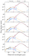 |
Fig. A.1. Best fit SED models of ALMA-selected galaxies. The black squares report the multiband photometric data. Flux upper limits at 5-σ for C1, C3, and C4, obtained from 3-mm continuum images are also reported. Red, blue, and orange lines represent the dust emission, and the young (star age <10 Myr) and old (>10 Myr) stellar components, respectively. The gray lines show random extraction from the posterior probability distribution of the total galaxy SED. |
Appendix B: Additional line emitters detected in the ALMA datacubes
In Fig. A.2. we report the additional line emitters corresponding to C2 (QSO-SE) and C6, respectively. Specifically, we detected the CO(4–3) line of C2 (QSO-SE) in the ALMA band 3 spectral scan targeting C4 (see, Sect. 4.3), and [CI]609 μm line of C6 in the band 6 datacube. We perform the fit of the lines and estimated line fluxes and luminosities by following the same approach described in Sect. 4.5, and report results in Table B.1.. We note that the C2 line emission is detected at the boundary of the FoV of the C4 pointing, therefore we corrected the spectrum for the PB response at the location of the source before modeling the line.
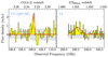 |
Fig. A.2. Spectra of additional line emitters identified in ALMA datacubes. Left panel: CO(4–3) line of C2 (QSO-SE) detected in the ALMA band 3 spectral scan of C4, corrected for the PB response. Right panel: [CI]609 μm line of C6 identified in the ALMA band 6 datacube. Data and the best-fit model are shown in yellow and red, respectively. The ±1σ RMS noise range of the data is indicated by the gray shaded area. The top scales report the expected line redshifts. |
Properties of the additional emission lines of the ALMA-identified sources.
All Tables
All Figures
|
Fig. 1. Footprints of ALMA observations toward the MUDF. Left panel: The background shows the HST/WFC3 F140W image, and the gray lines show the PB response of the ALMA band 6 mosaic at 30% and 50% (solid and dashed lines, respectively). The orange line indicates the region observed by VLT/MUSE with >3 hours of exposure time. Red diamonds indicate the MUDF quasar pair. The blue squares with labels indicate the high-fidelity ALMA-selected sources extracted from the 1.2 mm continuum image. The dot-dashed black circles show the ALMA pointings of the band 3 spectral scans toward three individual sources (P.C1, P.C3, and P.C4). The diameter of the circles indicates the HPBW at 101 GHz. Right panel: ALMA band 6 continuum observations. The synthesized beam size is shown in the bottom right corner. |
| In the text | |
|
Fig. 2. Sensitivity (RMS) of the ALMA band 3 spectral scans across the covered frequency range. Top panel: The colored curves and the right axis report the atmospheric transmission from the ALMA site at different levels of PWV obtained using plotAtmosphere task in the CASA analysisUtils package (Hunter et al. 2023b). The top axis reports the expected redshift of the CO(3–2) line. Bottom panel: Disposition of SPWs in the four frequency tunings. Vertical dotted lines indicate the edges of the SPWs. The maximum sensitivity is achieved within z≈2.35−2.5 where two SPWs in different frequency tunings overlap. The right axis reports the redshift of the various CO transitions (dash-dotted lines) covered by the spectral scan within z≃1−4. |
| In the text | |
|
Fig. 3. 5″×5″ postage stamps of NIR and optical/NUV counterparts of ALMA 1.2-mm continuum-selected sources in the MUDF. From left to right: 1.2-mm continuum map from ALMA band 6, HST/WFC3 F140W (central observed wavelength 1.4 μm), MUSE white light image (central observed wavelength 655 nm). The solid contours show the [2, 3, 2n]×RMS (with n≥2) levels of the ALMA continuum. The yellow ellipse at the corner of the bottom left panel shows the synthesized ALMA beam. |
| In the text | |
|
Fig. 4. Spectra extracted from ALMA band 3 spectral scans toward 1.2-mm continuum-selected sources C1, C3 and C4 (from the top to the bottom panel). Data and the best-fit model are shown in yellow and red, respectively. The ±1σ RMS noise range of the data is indicated by the gray shaded area. The top scale reports the expected CO(3–2) line redshift depending on the observed frequency. |
| In the text | |
|
Fig. 5. Connection between ALMA-selected galaxies and absorption systems in the spectra of the QSO-SE (black) and -NW (purple). The line-of-sight separations are centered on the redshift of the ALMA-selected galaxies. The vertical gray band indicates the velocity at which the optical depth of the absorption is 50% of the total (τ50). The transitions shown (C IV λ1548, Al II λ1670, and Mg II λ2796) are limited to the strongest lines among the multiple metals associated to each galaxy. Galaxies selected with ALMA are indicated by red diamonds with errorbars reporting uncertainties on their redshift measurements. The panels are ordered (from the top left to the bottom right panel) for increasing sky-projected separation (R) from the QSO sightline along which the absorption is detected. HST-selected galaxies linked to the same absorbers are shown with black triangles. The number of galaxies (Ngal) associated to each group (see, Sect. 5.3) is also reported. |
| In the text | |
|
Fig. 6. Star formation rate-stellar mass diagram of galaxies detected in the MUDF. The gray density contours show the distribution of all galaxies selected with HST in the rest-frame optical/UV at z∼1−2. The marginalized distributions of M★ and SFR are also shown on the top and right axis, respectively. The red density contours report the sample of SMG with photometric redshift within 1≤z≤2.5 from Dudzevičiūtė et al. (2020). The ALMA-selected galaxies with properties derived from SED modeling are reported with diamonds. Colored triangles mark the HST-selected group galaxies associated with the same absorption system of each ALMA-selected galaxy. The star-forming main sequence at z∼1−2 from Popesso et al. (2023) is also shown. |
| In the text | |
|
Fig. 7. Groups of galaxies around ALMA sources (blue squares). The colored triangles indicate the HST-selected galaxies belonging to the same group found around the redshift of ALMA sources (bottom left corner). The two quasars in the MUDF are labeled with red diamonds, the black arrow indicates the QSO sightline in which absorption at the redshift of each group is detected. The black crosses mark the projected location of the galaxy stellar mass-weighted barycenter of the groups. The gray solid and dashed lines report the PB response at 0.3 and 0.5, respectively, of the ALMA band 6 mosaic. |
| In the text | |
|
Fig. 8. Phase-space diagram of the galaxies identified with ALMA and of the other group members associated with quasar absorbers. The vertical axis reports the difference between the velocity shift from the absorption line center, measured from the τ50 wavelength (Δv(τ50)), and half of the Δv90 of the absorption profile. Negative values indicate that the galaxy systemic is near to the center of the absorption profile, while positive ones correspond to galaxies at the redshift of which no absorption is detected. The horizontal axis shows the galaxy impact parameters normalized by their virial radius (Rvir). The markers are color-coded as in Fig. 6. |
| In the text | |
|
Fig. 9. Galaxy surface density in groups as a function of EW of the associated absorbers (Mg II for C1, C6, and C7, and Al II for C3, respectively). Number density is computed by counting the number of galaxies (Ngal), and dividing for the effective area (Aeff) as described in Sect. 5.3. The associated uncertainties are obtained from Poisson statistics for low number counts (Gehrels 1986). The blue solid line and gray shaded area are the best fit linear model (Ngal/Aeff=a×(EW/Å)+b Mpc−2, with a = 4±2, b = 4±3) and 1σ confidence interval, respectively. The Spearman's rank correlation coefficient and the corresponding p-value are also reported. |
| In the text | |
|
Fig. A.1. Best fit SED models of ALMA-selected galaxies. The black squares report the multiband photometric data. Flux upper limits at 5-σ for C1, C3, and C4, obtained from 3-mm continuum images are also reported. Red, blue, and orange lines represent the dust emission, and the young (star age <10 Myr) and old (>10 Myr) stellar components, respectively. The gray lines show random extraction from the posterior probability distribution of the total galaxy SED. |
| In the text | |
|
Fig. A.2. Spectra of additional line emitters identified in ALMA datacubes. Left panel: CO(4–3) line of C2 (QSO-SE) detected in the ALMA band 3 spectral scan of C4, corrected for the PB response. Right panel: [CI]609 μm line of C6 identified in the ALMA band 6 datacube. Data and the best-fit model are shown in yellow and red, respectively. The ±1σ RMS noise range of the data is indicated by the gray shaded area. The top scales report the expected line redshifts. |
| In the text | |
Current usage metrics show cumulative count of Article Views (full-text article views including HTML views, PDF and ePub downloads, according to the available data) and Abstracts Views on Vision4Press platform.
Data correspond to usage on the plateform after 2015. The current usage metrics is available 48-96 hours after online publication and is updated daily on week days.
Initial download of the metrics may take a while.