| Issue |
A&A
Volume 694, February 2025
|
|
|---|---|---|
| Article Number | A67 | |
| Number of page(s) | 21 | |
| Section | Extragalactic astronomy | |
| DOI | https://doi.org/10.1051/0004-6361/202451093 | |
| Published online | 04 February 2025 | |
MusE GAs FLOw and Wind (MEGAFLOW)
XII. Rationale and design of a Mg II survey of the cool circum-galactic medium with MUSE and UVES: The MEGAFLOW Survey
1
Univ. Lyon1, ENS de Lyon, CNRS, Centre de Recherche Astrophysique de Lyon (CRAL) UMR5574, F-69230 Saint-Genis-Laval, France
2
Institut für Physik und Astronomie, Universität Potsdam, Karl-Liebknecht-Str. 24/25, 14476 Potsdam, Germany
3
Institute for Computational Astrophysics and Department of Astronomy & Physics, Saint Mary’s University, 923 Robie Street Halifax, Nova Scotia B3H 3C3, Canada
4
Institut de Recherche en Astrophysique et Planétologie, Université de Toulouse, Centre National de la Recherche Scientifique, Centre National d’Etudes Spatiales, 31028 Toulouse, France
5
European Southern Observatory (ESO), Karl-Schwarzschild-Str. 2, 85748 Garching b. München, Germany
6
Inter-University Centre for Astronomy & Astrophysics (IUCAA), Post Bag 04, Pune 411007, India
7
Leiden Observatory, Leiden University, PO Box 9513 NL-2300 RA Leiden, The Netherlands
8
Aix Marseille Univ., CNRS, CNES, LAM, Marseille, France
9
Canada-France-Hawaii Telescope, 65-1238 Mamalahoa Highway, Kamuela, HI 96743, USA
10
Leibniz-Institut für Astrophysik Potsdam (AIP), An der Sternwarte 16, 14482 Potsdam, Germany
⋆ Corresponding author; This email address is being protected from spambots. You need JavaScript enabled to view it.
Received:
12
June
2024
Accepted:
24
October
2024
Abstract
We present the design, rationale, properties, and catalogues of the MusE Gas FLOw and Wind survey (MEGAFLOW) of cool gaseous halos of z ≃ 1.0 galaxies, using low-ionisation Mg II absorption systems. The survey consists of 22 quasar fields selected from the Sloan Digital Sky Survey (SDSS), including multiple (≥3) strong Mg II absorption lines over the redshift range of 0.3 < z < 1.5. Each quasar was observed with the Multi-Unit Spectroscopic Explorer (MUSE) and the Ultraviolet and Visual Echelle Spectrograph (UVES), for a total of 85 hours and 63 hours, respectively. The UVES data resulted in 127 Mg II absorption lines over 0.25 < z < 1.6, with a median rest-frame equivalent width (REW) 3σ limit of ≈0.05 Å. The MUSE data resulted in ∼2400 galaxies, of which 1403 are characterised by a redshift confidence of ZCONF > 1; this amounts to more than 60 galaxies per arcmin2. They were identified using a dual detection algorithm based on both continuum and emission line objects. The achieved [O II] 50% completeness is 3.7−0.6+0.8 × 10⁻¹⁸ erg s−1 cm−2 (corresponding to an SFR of > 0.01 M⊙ yr−1 at z = 1) using realistic mock [O II] emitters and the 50% completeness is mF775W ≈ 26 AB magnitudes for continuum sources. We find that (i) the fraction of [O II] emitting galaxies that have no continuum is ∼15%; (ii) the success rate in identifying at least one galaxy within 500 km s−1 and 100 kpc is ≈90% for Mg II absorptions with Wr2796 ≳ 0.5 Å; (iii) the mean number of galaxies per Mg II absorption is 2.9 ± 1.6 within the MUSE field-of-view; (iv) of the 80 Mg II systems at 0.3 < z < 1.5, 40 (20) have 1 (2) galaxies within 100 kpc, respectively; and, finally, (v) all but two host galaxies have stellar masses of M⋆ > 109 M⊙ and star formation rates of > 1 M⊙ yr−1.
Key words: galaxies: evolution / galaxies: formation / intergalactic medium / quasars: absorption lines
© The Authors 2025
 Open Access article, published by EDP Sciences, under the terms of the Creative Commons Attribution License (https://creativecommons.org/licenses/by/4.0), which permits unrestricted use, distribution, and reproduction in any medium, provided the original work is properly cited.
This article is published in open access under the Subscribe to Open model. This email address is being protected from spambots. You need JavaScript enabled to view it. to support open access publication.
1. Introduction
The circum-galactic medium (CGM) is the complex interface between the intergalactic medium and the galaxies themselves. Traditionally, the CGM describes the gas surrounding galaxies outside their disks or interstellar medium and inside their virial radii (Tumlinson et al. 2017). The CGM is the interface between the continuous fresh source of fuel coming from the IGM and star-formation driven outflows, often referred to as the baryon cycle (Péroux & Howk 2020). As a result, the CGM is expected to retain the kinematical (and/or enrichment) signatures of these processes.
A significant amount of effort has been devoted to the study of galaxies close to quasi-stellar object (QSO) sight lines to study the interplay between outflows and accretion. The idea of such a medium goes back to the detection of cold gas clouds toward stars at high Galactic latitudes (Spitzer 1956). Soon after the discovery of the first quasars, Bahcall & Spitzer (1969) proposed that most of the absorption lines observed in QSO (quasar) spectra were caused by gas in the extended halos of normal galaxies.
The most commonly used metal absorption in quasar spectra is the magnesium (Mg II) λλ2796, 2803 doublet, which has been known to trace ‘cool’ (T ∼ 104 K) photoionised gas in and around galaxies since the studies of Bergeron & Boissé (1991), Bergeron et al. (1992, 1994), Steidel (1993), and Steidel et al. (1994). In the vicinity of galaxies, Mg II absorptions are expected to occur in sight lines, probing either outflows (as in Nestor et al. 2011) or accreting gas in extended gaseous disks (Fumagalli et al. 2011; Pichon et al. 2011; Kimm et al. 2011; Shen et al. 2013; DeFelippis et al. 2021). Strong Mg II absorptions, with REW  Å, can also occur in groups (e.g. Kacprzak et al. 2010; Gauthier 2013; Bielby et al. 2017) and weak Mg II absorptions (
 Å) in the outskirts of clusters (e.g. Mishra & Muzahid 2022).
The detection of tens of thousands of Mg II absorbers with  Å (e.g. Nestor et al. 2005; Zhu & Ménard 2013) thanks to the Sloan Digital Sky Survey (SDSS, York et al. 2000) have enabled large statistical analyses (e.g. Bouché et al. 2006; Lundgren et al. 2009; Gauthier et al. 2009). As noted in Nestor et al. (2005), the REW
  distribution is a double exponential, where the transition occurs at around
  Å, indicating a transition between strong and weak Mg II systems possibly related to different physical mechanisms. This is supported by the different redshift evolution of strong and weak Mg II systems (Nestor et al. 2005).
However, connecting the kinematics of the gas inflow and ouflow processes to the kinematics of the host galaxy requires us to be able to identify the host efficiently. The advent of the Multi Unit Spectroscopic Explorer (MUSE, Bacon et al. 2010) on the Very Large Telescope (VLT) has revolutionised the study of the CGM thanks to its exquisite sensitivity and its field of view (FOV). As a result, a number of MUSE-based CGM surveys have been developed over the past few years, such as QSAGE (Bielby et al. 2019), MUSEQuBES (Muzahid et al. 2020), CUBES (Chen et al. 2020), MAGG Lofthouse et al. (2020), and MUSE-ALMA (Péroux et al. 2019).
This paper describes the rationale, design, and properties of the MusE GAs FLOw and Wind (MEGAFLOW) survey, a Mg II-selected survey around 22 QSO fields. This paper is part of a series of 13 papers (Schroetter et al. 2016, 2019, 2021, 2024; Zabl et al. 2019, 2020, 2021; Wendt et al. 2021; Freundlich et al. 2021; Langan et al. 2023; Cherrey et al. 2024; Cherrey et al. 2025) and it is organised as follows. In Sect. 2, we present the survey design and rationale. For each of the 22 quasar fields, we have obtained MUSE observations (from 2 to 11 h) and high-quality UVES spectra, as discussed in Sect. 3. In Sect. 4, we present the methods used to generate the catalogs of Mg II absorbers and galaxies. In Sect. 5, we describe the physical properties of the galaxies. In Sect. 6, we present the main properties of the host galaxies. In Sect. 7, we compare our sample to others from the literature. Our conclusions are given in Sect. 8.
Throughout this paper, we use a Λ cold dark matter (ΛCDM) model with ΩM = 0.307, ΩΛ = 0.693, and H0 = 67 km s−1 Mpc−1 (‘Planck 2015’ Planck Collaboration XIII 2016). At the typical redshift of our survey, z = 1, 1″ corresponds to 8.23 kpc. All magnitudes are in the AB system.
2. MEGAFLOW survey design and rationale
The low-ionisation Mg IIλλ2796, 2803 doublet seen in quasar spectra has been recognised as a good tracer of the cool (T ∼ 104 K) CGM for close to thirty years now (e.g. Bergeron & Boissé 1991; Bergeron et al. 1992; Steidel et al. 1995, 1997, 2002). However, finding the galaxy counterpart associated with the Mg II absorption is often a complicated process. Before the advent of integral field spectrographs (IFS), this required deep pre-imaging to identify host-galaxy candidates and expensive spectroscopic follow-up campaigns to secure the host galaxy identification from its redshift (e.g. Bergeron & Boissé 1991; Steidel et al. 1997; Chen & Tinker 2008; Chen et al. 2010a,b; Churchill et al. 2013; Nielsen et al. 2013a,b). Still, the imaging+spectroscopy technique suffers from several disadvantages: (i) it is inefficient, requiring multiple campaigns for imaging, redshift identification, and kinematics determinations (e.g. Kacprzak et al. 2011; Ho et al. 2019; ii) it is biased against emission-line galaxies given that pre-imaging necessary for the pre-identification of host-galaxy candidates is based on the continuum light; and (iii) it is challenging close to the line-of-sight (LOS) due to the quasar point spread function (PSF).
These shortcomings can be bypassed using Integral Field Unit (IFU) spectroscopy such as SINFONI (Eisenhauer et al. 2003) or the MUSE instrument (Bacon et al. 2010) given that an IFU allows the identification of the galaxy counterpart without pre-imaging, as demonstrated in Bouché et al. (2007). In addition, IFU observations also provide the host kinematics and the morphological information which are both easily determined from such 3D data. Furthermore, 3D data offers the possibility to easily subtract the quasar’s PSF.
The exquisite sensitivity and large field-of-view (1′×1′) of MUSE allows us to detect galaxies further from the quasar (30″ or ∼250 kpc at z = 1). Its broad wavelength coverage (4700 Å to 9300 Å) allows us to target quasar sight lines with multiple Mg IIλλ2796, 2803 absorption lines over the redshift range from 0.4 to 1.5, which are suitable for the identification of [O II] emitting galaxies.
The MEGAFLOW survey is aimed at building a statistical sample with at least 100+ galaxy-quasar pairs (i.e. 10× larger than our SINFONI survey, Bouché et al. 2007) to allow for a robust analysis of the relation between the absorption and the host galaxy properties. To this end, we selected quasars with (i) at least three (Nabs ≥ 3) Mg IIλλ2796, 2803 absorption lines at redshifts between 0.4 and 1.4, ensuring that a sample ∼100 galaxy-quasar pairs could be build with only 20–25 quasar LOS; and (ii) with a REW  Å from the Zhu & Ménard (2013) Mg II catalogue of 100 000 Mg II absorption lines extracted from 400 000 quasar spectra in SDSS (DR12)1. The latter criterion ensures that the host galaxies are within 100 kpc from the quasar LOS (at z ∼ 1), namely, within the MUSE field of view, given the well known anti-correlation between the impact parameter and rest-frame equivalent width of
  (Lanzetta & Bowen 1990; Steidel 1995).
Ultimately, the MEGAFLOW survey is comprised of 22 quasar fields listed in Table 1 and the above selection criteria resulted in a sample of 79 Mg II absorbers with  Å. This survey is thus optimised to study the properties of galaxies associated with strong Mg II absorption lines, but given the wide wavelength range, it has also allowed us to perform a galaxy-centred analysis, including, for example, the covering fraction of Schroetter et al. (2021) and Cherrey et al. (2024, 2025). We discuss the impact of the MEGAFLOW selection criteria on such analyses in Sect. 6.6.
MEGAFLOW quasar fields.
As part of the MEGAFLOW series, in Schroetter et al. (2016, 2019), we presented a preliminary analysis on quasars probing galactic outflows. In Zabl et al. (2019), we presented a preliminary analysis on quasars probing extended gaseous disks, based on a first version of the galaxy catalog, referred to as ‘DR1’. In Zabl et al. (2020), we presented a first tomographic study of an outflow probed by two background sources. In Zabl et al. (2021), we presented an extended Mg II map of the outflowing material around a z = 0.7 star-forming galaxy. In Wendt et al. (2021), we presented a first analysis of the metallicity/dust content of the CGM as a function of azimuthal angle. In Schroetter et al. (2021), we presented a first analysis on the Mg II and C IV covering fractions at z > 1. In Freundlich et al. (2021), we presented a first attempt at detecting the molecular gas content of a subset of galaxies. In Langan et al. (2023), we presented an analysis of the impact of gas in/outflows on the main-sequence and mass-metallicity scaling relations. In Cherrey et al. (2024), we presented an analysis of the Mg II covering fractions in groups of galaxies. In Cherrey et al. (2025), we presented an analysis of the Mg II covering fraction of isolated galaxies.
3. Data
In Section 3.1, we describe the MUSE data and data reduction. In Section 3.2, we describe the UVES data reduction.
3.1. MUSE data
The MUSE observations were conducted in visitor mode between 2014 and 2018 using guarantee time observations (GTO). The data were acquired in wide field mode (WFM), using both standard (WFM-NOAO-N) and adaptive-optics (WFM-AO-N) modes; the latter has been available since Fall 2017, following the commissioning of the ground layer adaptive optics (AO) facility. Given that the AO observations have a gap at 5800–5980 Å due to the AO notch filter, some of the combined (AO+ non-AO) datasets have a very heterogeneous PSF in that spectral region. The programme IDs, total exposure times, and the final image quality data are listed in Table 2.
Summary of MUSE observations for the 22 fields.
To produce a fully calibrated 3D-cube, we used the standard recipes from the MUSE data reduction pipeline (version ≥2.4, Weilbacher et al. 2014, 2020) and supplemented some post-processing with custom routines following Bacon et al. (2017, 2023) and Zabl et al. (2019) with some differences. The sequence of steps is illustrated schematically in Fig. 1.
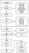 |
Fig. 1. Schematic diagram of the steps in the data reduction process. |
First, raw night calibration exposures were combined to produce a master bias, master flat, and trace table (which locates the edges of the slitlets on the detectors). These calibrations were then applied to all the raw science exposures with the scibasic recipe. Bad pixels corresponding to known CCD defects (columns or pixels) were also masked to reject known detector defects. Subsequently, the scibasic recipe performed the required geometric and wavelength calibrations. At this point, the pipeline product is a pixel table (hereafter called pixtable) containing all pixel information: location, wavelength, photon count, and an estimate of the variance.
While the flat-fielding with lamp flats done in the scibasic step removes any pixel-to-pixel sensitivity variations, it is not sufficient to ensure an even illumination, especially across the different IFUs. Twilight exposures and night-time internal flat calibrations (called illumination corrections) are used (when available) for additional correction in order to correct for these flux variations at the slice edges (depending on the ambient temperature). We always used the illumination taken at a similar time and/or with an ambient temperature closer to that of the science exposures.
Next, the scipost recipe performed the atmospheric dispersion correction, barycentric velocity correction, astrometric calibration, telluric correction, and flux calibration on the pixtable. Regarding the flux calibration, observations of spectro-photometric standard stars were reduced in the same way as the science data (save the flux-calibration). The spectral response function used for flux-calibration of the science data was determined by comparing the star’s spectrum to tabulated reference fluxes.
As described in Bacon et al. (2023, their Fig. B1), we can still see a low-level footprint of the instrumental slices and channels that arises from imperfect flat-fielding, which are difficult to correct for with standard calibration exposures, as illustrated on Fig. 2a. The procedure (referred to as ‘auto-calibration’) to correct for this starts by masking all bright objects in the data using the white-light image as described in the Appendix B.2 of Bacon et al. (2023). The algorithm calculates the median background flux level in each slice (before sky-subtraction) using only the unmasked voxels and then scale all slices to the mean flux of all slices using a robust outliers rejection (15σ clipping of the median absolute deviation). This slice normalisation is done in 20 wavelength bins of 200–300 Å chosen so that their edges do not fall on a sky line. This self-calibration approach is implemented in the MUSE pipeline for versions ≥2.4 (see Sect. 3.10.2 of Weilbacher et al. 2020).
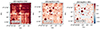 |
Fig. 2. White-light images (variance weighted) for the field J0014p0912 from different data-reductions. Left: Automatic data reduction from ESO. Middle: Data reduction (‘DR1’) using custom scripts as in Zabl et al. (2019). Right: Final data reduction (‘DR2’) used here using super flats (Sect. 3). |
Processing the data up to this point (box in Fig. 1) is standard, performed with the default parameters of the pipeline within the MuseWise framework2 (Valentijn et al. 2017). This stage includes the removal of the sky telluric emission (OH lines and continuum) and of Raman lines induced by the lasers from the AO facility (Weilbacher et al. 2020, Sect. 3.10.1).
One remaining imperfection, even after the flat fielding steps and the per-slice auto-calibration, are sharp flux drops at the edge of slices that are located at edges of the IFUs. As discussed in Bacon et al. (2023, their Appendix B.4), a way to improve upon these remaining imperfections is through the use of pseudo ‘skyflats‘ (or superflats) generated from multiple exposures. This procedure requires to resample the pixtable into a cube sampled on the same instrumental grid by turning off the dithering and rotations. This means that in order to create a skyflat for each exposure, we need to resample all of the others (used as skyflat) to the grid of that exposure. Given that we need around 30 sky exposures to create a skyflat, the required amount of re-sampling is computationally very expensive.
To avoid this expensive computational effort, we created the pseudo skyflats from the scipostpixtable level, just before resampling the cubes. The pixtables produced by scipost contain fully flux calibrated (including all flat field steps described above) and we stacked these pixels. One practical necessity is to mask objects which are in the sky-exposures in the pixtables. The assumption here is that the flat-fielding imperfections, which we aim to catch with the sky-flat, do not shift around on the detector.
The most suitable exposures for constructing the sky-flats are observations of extragalactic deep fields, as they have a relatively sparse source density and, hence, a substantial free sky coverage. To have a sufficient signal to form a skyflat, we needed 30–50 frames. In total, we constructed four sky-flats for the GTO runs in Oct.–Nov. 2014, Sep.–Oct. 2015, Jan.–Feb. 2017, and Aug. 2018, from various deep field observations taken as part of MUSE GTO programmes, spanning the bulk of the observations. Once created, we were able to subtract this sky-flat from each of the science exposures in detector-coordinates at the pixtable level. For cases where the sky-flats did not perform well, we decided to mask instead the regions with imperfect flat-fielding (again in the pixtable) before resampling. Then, we masked the rare cases of individual slices with problems (e.g. due to some problem with the sky subtraction) in the pixtable, as well as any satellites that were identified from white-light images create from a first pass reduction.
A datacube was then created from the skyflat corrected pixtables with the pipeline recipe scipost, using the default 3D drizzling interpolation process. We resampled all exposures of a field individually specifying a common output WCS. We then performed quality control for each exposures, including measurements of the PSF and flux. We rejected any exposures where the flux calibration was off (e.g. due to clouds) or where there was a significantly worse seeing than the majority of the exposures in the field.
With the offsets between exposures to correct for the de-rotator wobble, computed on white-light images constructed from the pixtables, we produced data-cubes resampled to the same WCS pixel grid for each exposures. These individual data-cubes were finally combined using MPDAF (Piqueras et al. 2019). This allowed us to perform an inverse-variance weighted average over a large number of data-cubes. A 3–5σ rejection (depending on the number of exposures) of the input pixels was applied in the average to remove remaining badpixels and cosmic rays.
The combined datacube was finally processed using the Zurich Atmospheric Purge (ZAP Soto et al. 2016) version 2.03 described in Bacon et al. (2021, Appendix B.3). ZAP performs a subtraction of remaining sky residuals based on a principal component analysis (PCA) of the spectra in the background regions of the datacube. We provide as input to ZAP an object mask generated from the white-light image of the combined cube with SEXTRACTOR (Bertin & Arnouts 1996) to remove the fluxes from all the bright objects.
The cubes were corrected for galactic extinction using the all-sky thermal dust model from the Planck mission (Planck Collaboration XI 2014). Specifically, we used the DUSTMAPS Python interface (Green 2018)4 to get the galactic color excess E(B − V) from the Planck data. We then corrected the cube using the Cardelli et al. (1989) extinction curve with RV = 3.1. This ensures that all spectra and flux measurements in the catalogues will be properly dust-corrected. This cube is referred to as the beta dataset.
In addition, we also produced a version of the cube after subtracting the QSO PSF using PAMPELMUSE5 (Kamann et al. 2013) for the non-AO fields and using the Modelisation of the AO PSF in Python tool MAOPPY6 (Fétick et al. 2019) for the fields taken with AO. This cube is referred to as the psfsub dataset.
3.2. UVES quasar spectra
The quasars of this MUSE GTO-Program were all observed with the high-resolution spectrograph UVES (Dekker et al. 2000) between 2014 and 2018 (see Table 3). The settings used in our observations were chosen in order to cover the Mg IIλλ2796, 2803 absorption lines as well as other elements such as Mg Iλ2852, Fe IIλ2586 when possible. Additional observations were carried out in cycle 108 (2021, 2022) to fill some gaps in redshift coverage for certain sight lines and in particular weak ions. The total observing time amounts to 59 h (63 h, including archival observations from 2004).
Summary of UVES observations for the MEGAFLOW fields.
The data were taken under similar conditions resulting in a spectral resolving power of R ≈ 38 000 dispersed on pixels of ≈1.3 km s−1. The Common Pipeline Language (CPL version 6.3) of the UVES pipeline was used to bias correct and flat field the exposures and then to extract the wavelength and flux calibrated spectra. After the standard reduction, the custom software UVES Popler (Murphy 2018, version 1.05 from Sept. 2020) was used to combine the extracted echelle orders into single 1D spectra in vacuum wavelength. The continuum was fitted with low-order polynomial functions Murphy et al. (2019).
Figure 3 shows the median 3-σ limit as a function of redshift for the 22 quasar spectra (black line). The gray lines represent the 10th and 90th percentiles, while the blue lines represent the 25th and 75th percentiles. The
  limits were obtained from the uncertainty per pixel σpix, the average line width of a weak Mg IIλλ2796, 2803 absorption wMgII = 5 km s−1, the pixelsize pix = 1.3 km s−1, the local pixel width dl in Å, and the detection significance = 3 using
 (1)
(1)
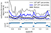 |
Fig. 3. Median 3σ REW limits for Mg II 2796 as a function of redshift for all 22 UVES spectra (solid black line). The blue and grey lines represent the 25th and 75th percentiles, respectively. Figure A.1 shows the REW limits for each field individually. The bottom graph shows the number of sight lines covering each redshift. |
4. Catalogues
In this section, we present the making of the absorption line catalogues (Sect. 4.1) and of the galaxy catalogues (Sect. 4.2).
4.1. Mg II absorption lines
As discussed in Sect. 2, the SDSS survey selection (DR1) yielded 79 Mg II absorption lines in the 22 QSO fields selected from SDSS spectra, which we refer to as the ‘DR1’ absorber sample. These lines were used in past studies, such as those of Schroetter et al. (2019), Zabl et al. (2019), and Wendt et al. (2021). In addition, we searched for serendipitous Mg II absorbers in our UVES spectra, and found an additional 48 Mg II absorption lines, leading to a total of 127 Mg II absorption lines, which is referred to as the ‘DR2’ sample.
The additional absorption lines were found independently by the two members of the team (IS and SM). First, the wavelength array of each spectrum is shifted by the rest-frame wavelength ratio (2796.3543/2803.5315) of the Mg II doublet. The shifted spectrum is then plotted on top of the original spectrum. Such a shift will translate the absorption corresponding to the weaker member of the doublet (Mg II 2803) to the location of the stronger member (Mg II 2796), since the ratio of observed wavelengths is equal to the ratio of the rest-frame wavelengths, it is independent of redshift. We took note of such coincidences in each spectrum and determined their redshifts. We then made velocity plots for each of these putative Mg II systems to verify the presence or absence of other prominent transitions such as the Fe II, Ca II, Mn II, and C IV. However, the presence of these absorption lines was not mandatory for an absorber to be deemed as Mg II. The final Mg II catalogue was then built by mutual agreement between IS and SM, considering factors such as the detection significance, velocity structures of the two transitions, and contamination.
The final Mg II absorption catalogue (DR2) contains 127 Mg II absorption lines and the list can be found on the AMUSED7 and MEGAFLOW8 websites. Figure 4 (top) compares the redshift distribution of the full Mg II absorption line sample (grey histogram) to the pre-selected absorption lines (solid histogram). Figure 4 (bottom) compares the rest-frame equivalent width (REW)  Mg II distributions of the full sample (dotted histogram) to the SDSS pre-selected sample (solid histogram). The grey histogram represents the DR2 sample after matching the redshift distribution of the DR1 sample. For comparison, the Nestor et al. (2005) and Zhu & Ménard (2013) power laws for the REW distribution of z = 1 Mg II are shown (normalisation is arbitrary). The dotted line represents a fit to the DR2 sample at 0.4 < z < 1.5 and for REW greater than
  Å, along with its 95% confidence interval obtained from 5000 bootstrap fits. The MEGAFLOW Mg II absorption lines REW distribution has the same slope as random QSO fields, albeit with a different normalisation, as pointed out in Schroetter et al. (2021, their Fig. A.3). Indeed, the MEGAFLOW ∂N/∂Wr ∝ exp(−Wr/a) with
  which is consistent with a = 0.77 ± 0.01 from field statistics (Nestor et al. 2005; Abbas et al. 2024) for strong absorbers.
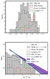 |
Fig. 4. Properties of the Mg II absorption catalogue. Top: Redshift distribution of the Mg II absorption systems. The solid and gray histograms show the absorbers for the SDSS (DR1) and UVES (DR2) selections, respectively. Bottom: Rest-frame equivalent width |


4.2. Galaxies
In the section below (Sect. 4.2.1), we discuss the DR1 catalogue of [O II] emitters associated with the 79 Mg II absorption lines. The DR1 catalogue is the basis of the analysis in Schroetter et al. (2019), Zabl et al. (2019, 2020, 2021), Wendt et al. (2021) and Freundlich et al. (2021). In Sect. 4.2.2, we discuss our DR2 catalogue of all galaxies, which consists of a dual selection of [O II] line emitters and continuum-selected sources at all redshifts. A preliminary version of this catalogue was used in the analysis presented in Langan et al. (2023) and Cherrey et al. (2024).
4.2.1. DR1: [O II] emitters at zabs
As discussed in Zabl et al. (2019), the redshift identification of galaxies associated with the 79 Mg II absorption lines was based on multiple pseudo narrow-band (NB) images of width ≈400 km s−19 suitable for [O II], [O III] and Hβ emitters extracted from an early data reduction of the dataset (Zabl et al. 2019). Each NB image is continuum subtracted by using two off-bands, and the NB images are combined in a single NB image (S/N weighted). We then automatically search for low-S/N objects in these NB images using the detection algorithm SEXTRACTOR (Bertin & Arnouts 1996). We also searched for quiescent galaxies by creating pseudo-NB images around the Ca H&K doublet. We ran SEXTRACTOR on the inverted NB image given that quiescent galaxies at the right redshift have negative fluxes in the continuum-subtracted images. Finally, we manually checked each candidate. This procedure consisted in a sample of 168 galaxies associated with the 79 absorbers, which is referred to as the ‘DR1’ galaxy sample.
4.2.2. DR2: blind [O II] emitters
With ∼90 000 optical spectra per single pointing, there is visible demand for automatic source detections such as the Line Source Detection and Cataloging (LSDCat) algorithm (Herenz & Wisotzki 2017) or ORIGIN software (Mary et al. 2020). LSDcat is a matched filtering and thresholding algorithm for emission lines algorithm written for IFU data and used for single emission lines such as Lyα emission lines. After the filtering process, the elements in the data cube represent the statistical S/N an emission line at that voxel position would have given that it was perfectly represented by the filter template and also assuming fully Gaussian, uncorrelated noise. The resulting signal is quite robust against varying spectral or spatial sizes of the single-line template. Hence, LSDcat has also been proven quite effective at indicating other emission features than pure Lyα. A simple ‘thresholding-approach’, however, is prone to spurious detections, namely, the so-called false positives that directly depend on the threshold.
Here, we use the Find Emission LINE objects (FELINE10) algorithm from Wendt et al. (2024), which combines a fully parallelised galaxy line template-matching with the matched filter approach for individual emission features of LSDcat. For the 3D matched filtering, the complete data cube is first median filtered to remove all continuum sources, and then cross-correlated with a template of an isolated emission feature in two spatial and one spectral dimension. We assumed a simple Gaussian with a FWHM of 250 km/s for the line profile and a PSF based on the given seeing in the data cube.
The FELINE algorithm then evaluates the likelihood in each spectrum of the cube for emission lines at the positions provided by a given redshift and a certain combination of typical emission features. FELINE probes all possible combinations of up to 14 transitions paired in 9 groups: Hα, Hβ, Hγ, Hδ, [O II], [O III], [N II], [S II], and Ne III for the full redshift range of interest (0.4 < z < 1.4). This particular selection of lines is motivated by the most prominent emission features expected in the MUSE data within this redshift range. This results in 512 (29) different models that are assessed at roughly 8000 different redshifts for each of the ≈90 000 spectra in a single data cube. To ensure that only lines above a certain S/N threshold contribute to each model, a penalty value is subtracted for each additional line. The S/N near strong sky lines are set exactly to that threshold. Therefore, lines that fall onto such a contaminated region will not affect the model quality. This is particularly useful for doublet lines that then contribute to a model, even when one of the lines aligns with a skyline. For each spaxel, the model with the highest accumulative probability over all contributing lines and its corresponding redshift are determined. This approach has the benefit to pick up extremely weak emitters that show multiple emissions lines, while avoiding the deluge of false positives when looking for single lines below a certain S/N threshold. This can be applied to each spatial element independently and was thus fully parallelised. From the resulting spatial map of best model probabilities, the peaks were automatically selected via maximum filter and 1D spectra were extracted for each emission line galaxy candidate. Those extracted spectra were fitted with an emission line galaxy template and with the redshift, as well as the individual line strengths; the latter is the only free parameter to reach sub pixel accuracy in an early redshift estimate and deriving further diagnostics for the later manual inspection, such as the [O II] line ratio.
Several of us (JZ, IS, SM, MW, and NB) visually inspected the FELINE solutions with a custom tool and rated each object according to the likelihood of being an [O II] emitter. The score was ‘A’ for a clear identification of an [O II] emitters, ‘B’ for likely [O II] emitters (due to weak S/N or marginally [O II] doublet resolved), and ‘No’ for real objects other than [O II] emitters. A special flag ‘X’ was used when the redshift solution was wrong or needed to be discussed and resolved. The scores (A/B/No/X) were converted to numerical values (2/1/0/-9) and averaged. The FELINE data products are made of the list of FELINE sources (along with the source masks) with their average (and dispersion) [O II] scores.
4.2.3. DR2: continuum sources
We use SEXTRACTOR (Bertin & Arnouts 1996) on the white-light images extracted from each datacube to identify continuum-selected sources. For each field, we optimised the detection parameters. Typically, we used a minimum area of 6–8 spaxels, with a S/N threshold of ≈1.0–1.3, Gaussian kernel of FWHM 2 spaxels, a deblending threshold of 64 levels, and an automatic background subtraction.
4.3. Completeness
We estimated the completeness of our data by adding N = 150 fake [O II] emitters in two versions of one of our MUSE fields (J0937p0656), using a shallow (2.3 h) and the deepest (11.2 h) version. The [O II] emitters were placed at five wavelengths (∼505, 605, 705, 820 and 920 nm) selected to be away from sky emission lines and spatially distant from known sources. The emitters are generated using the GALPAK3D algorithm using the measured PSF and with realistic galaxy parameters for [O II] emitters covering a range of redshifts, inclinations, fluxes and surface brightnesses. Specifically, we used an inclination, i, selected according to a uniform distribution sin(i) ∝ 𝒰(0.5,0.95) over the range of i = [30, 75] deg; position angles uniformly from 𝒰(0,360); (turbulent) velocity dispersion σ0 = 25 km s−1; tanh rotation curve with Vmax = 100 km s−1 and turn-over radius of rv = Re/1.26 (following Amorisco & Bertin 2010; Bouché et al. 2015); half-light radii, Re, of 2.5 and 5 kpc; [O II] doublet ratios randomly selected from a normal distribution 𝒩(0.8,0.1); flux profiles with Sérsic index n = 1; and total fluxes of [1, 2, 4, 6, 8, 10] × 10−18 erg s−1 cm−2.
We ran FELINE on the shallow and deep cubes with fake sources. The completeness function, fc, was then defined as the fraction of sources detected. Because fc is a complex function of 3D surface brightness in the spatial x, y and in the wavelength directions, it traditionally requires generating a large number of fake sources (over several detection runs), which then requires binning the results in wavelength, sizes, flux, and so on. Instead, we used the Bernoulli regression suitable for binary outcome developed in Bouché & McConway (2019) and presented in Schroetter et al. (2021), which has the advantage that it requires no binning. Briefly, for a set of fake sources, the detectability Yi is either 0 or 1, and the method consists in parametrising the completeness function, fc, which ranges from 0 to 1, as a Logistic function L(t)≡1/[1 + exp(−t)] where the function t = F(Xi; θ) is any linear combination of the independent variables: Xi, t = α + β1X1 + ⋯ + βnXn. The Bayesian algorithm then optimises the parameters using a Bernoulli likelihood against the observed series of detected and undetected sources, Yi. We used the No-U-Turn Sampler from (Hoffman & Gelman 2014, NUTS), a self-tuning Hamiltonian Monte Carlo, implemented in the python probabilistic package PYMC3 (Salvatier et al. 2016). For the logistic function L, we use F as a function of flux f, size R, and wavelength λ, namely:
![Mathematical equation: $$ \begin{aligned} F(X_i;\theta ) =A[ \log f_i +\mathrm{ZP}(\lambda )] + B (\log R_i-\log \overline{R}) \end{aligned} $$](/articles/aa/full_html/2025/02/aa51093-24/aa51093-24-eq21.gif) (2)
(2)
where A defines the sharpness of the Logistic function L(t), B the size dependence, and ZP(λ) is the wavelength-dependent 50% completeness, taken as a third-order polynomial ZP(λ) = C + α(λ − λ0)+β(λ − λ0)2 + γ(λ − λ0)3. Here, λ0 ≡ (1 + z0)×3727 Å is the reference wavelength for [O II] emitters at a redshift of z0 = 1.
Figure 5 shows the completeness achieved for [O II] emitters in the J0937+0656 data as a function of wavelength and redshift (panel a) and as a function of flux and size (panel b). The fitted parameters are listed in Table 4 which indicates that the 50% completeness for [O II] emitters at λ0 ≈ 7000 Å is 3.7 erg s−1 cm−2 (7.07
 erg s−1 cm−2) in the deep (shallow) cubes.
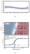 |
Fig. 5. Completeness for [O II] emitters in the deep cube J0937+0656. (a) Completeness level (50%) as a function of redshifts. (b) Completeness as a function of size Re (top panel) and [O II] fluxes (bottom panel). The red (blue) squares represent the [O II] emitters detected (not detected), respectively. The shaded area represents the fit to the unbinned data. |
Regarding the completeness of continuum sources, we estimated the completeness from the number counts (N/deg2/0.5mag) shown in Fig. 6 (left). By fitting the F775W number counts normalised to the expected counts from large galaxy surveys, such as the recent GAMMA/DEVILS survey (Koushan et al. 2021), we find that the 50% completeness is mF775W ≈ 25.2 mAB the shallow fields (2–4 h) and is mF775W ≈ 26 mAB for the two deep fields (11 h).
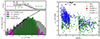 |
Fig. 6. Magnitude distributions for the DR2 catalogue. Left: Magnitude F775W number counts. The grey histogram represents the entire MEGAFLOW survey. The magenta histogram represents the 20 shallow fields and the green histogram the 2 deep fields. Compared to the number counts from the GAMMA/DEVILS survey (solid line) from Koushan et al. (2021), the MEGAFLOW survey is 50%-complete to i ≈ 25.2 mAB (26 mAB) in the shallow (deep) fields, respectively. Right: Magnitude-redshift distribution of all sources with redshifts z > 0. The QSOs are shown as grey circles. The galaxies with ZCONF = 1 (2,3) are represented as green circles (blue squares), respectively. |
4.4. Source inspection
At this point, each source in the FELINE and continuum-based catalogues were assigned a 6-digit FELINEID or WHITEID, using the following nomenclature: ‘xxa001’. Here, ‘xx’ is the unique field ID (Table 2) and ‘a’ is 0 for FELINE source, 1 for continuum sources, and 2 for continuum sources near the QSO, in the psfsub dataset.
Following Bacon et al. (2023), we used the PYMARZ software (Hinton et al. 2016) to identify five redshift solutions for the FELINE and continuum sources with nine templates for passive and star-forming galaxies and then used PYPLATEFIT11 to perform an emission and absorption line fitting on each of the redshift solution. We also computed the narrow-band images associated with each emission or absorption lines with S/N > 2 packaged in ‘source’ fits files, which are important to assess the detection of weak lines. The FELINE, PYMARZ redshift solutions, the fitted lines with S/N > 2, narrow-band images, and spectra are all used to produce static html files as in Bacon et al. (2023, their Fig. 19).
These static html files are then fed into a modified version of the SOURCEINSPECTOR tool (Bacon et al. 2023), a Python-Qt interface that allow users to select one of the redshift solutions or to provide a new one. However, most importantly, the SOURCEINSPECTOR tool allows the user to match continuum-detected sources with FELINE-detected sources (and vice versa) with confidence.
4.5. Categories for inspection
At this stage, the catalogue contains a high fraction of false detections to make sure it is highly complete. The removal of the false detections requires an inspection. To optimise the time required for inspecting the catalogues with SOURCEINSPECTOR, we pre-matched the FELINE and continuum sources and focussed on galaxies at 0.4 < z < 1.4 that are likely to either be star-forming galaxies with [O II] or passive galaxies with just continuum. Specifically, we cross-matched the FELINE and continuum catalogues according to their RA, Dec and defined the following categories:
-
1.1 ‘GoodFelineCont’ sources with FELINE score of ≥1.0 and continuum detection;
-
1.2 ‘GoodFelineNoCont’ sources with FELINE score of ≥1.0 and no continuum detection;
-
1.3 ‘GoodFelineNoMarz’ sources with FELINE score of ≥1.0, whose redshift is not among the 5 MARZ solutions within 150 km/s;
-
2.1 ‘BrightContGoodFeline’ bright continuum sources with magAUTO of < 24.5 (25.0 for the two deep fields);
-
2.2 ‘BrightContNoFeline’ bright continuum sources without a FELINE match;
-
3.0 ‘FelineBorderLine’ sources with FELINE score between 0.5 and 1.5; or with a score standard dispersion of > 0.45;
-
4.0 ‘Other’ sources that are not in the other categories.
For instance, for the deep field J0014−0028, there are 289 FELINE sources and 251 continuum sources and they are distributed in each category as follows:
-
1.1 GoodFelineCont 66
-
1.2 GoodFelineNoCont 23
-
1.3 GoodFelineOffMarz 18
-
2.1 BrightContGoodFeline 30
-
2.2 BrightContNoFeline 31
-
3.0 FelineBorderline 46
-
4 Other (FELINE) 180; and Other (Cont) 190.
Several of us (MW, IS, JZ, RB, NB, SM, and JR) inspected the redshift solutions for the categories 1.x, 2.x, and 3.0 with SOURCEINSPECTOR, where each member assessed the redshift confidence (ZCONF) ranging from 0 to 3.
A confidence level of ZCONF=0 corresponds to the situation where no redshift solution was found. A confidence level of ZCONF=1 corresponds to a low confidence solution, namely, when the redshift solution remains uncertain (could be [O II] or Lyα) owing to the low S/N of the line. A confidence level of ZCONF=2 corresponds to a high S/N single line whose shape is identifiable (e.g. a resolved [O II] doublet, an asymmetric Lyα). A confidence level of ZCONF=3 corresponds to a secure redshift with multiple lines.
4.6. Reconciliation
The results of the visual inspections were then combined and when there were several different redshift solutions proposed, we resolved the disagreement during the reconciliation meetings. The inspection and reconciliation process also yielded some sources that required to be split (in cases where the SEXTRACTOR deblending failed) or to be merged (in cases where FELINE assigned two redshifts due to a large kinematic gradient). The entire sequence of steps in the process were processed with custom routines forming the MegaFlow Catalog Processor (MFCP), which is based on MUSEX used in Bacon et al. (2023). The sequence is illustrated in Fig. 7. As discussed in Sect. 4.5, the entire process is optimised for galaxies at z < 1.5 and is somewhat biased against Lyα emitters that fall into the category ‘4’, which were not systematically inspected.
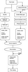 |
Fig. 7. Schematic illustration of the process used to generate the final catalogue from the FELINE and continuum-based catalogues. |
4.7. Final DR2 catalogue
The final catalogue (v2.0) contains 2427 sources, which includes 22 quasars, 57 stars, 1998 galaxies with ZCONF ≥ 1, and 350 sources with no redshifts (ZCONF = 0). The statistics of ZCONF in the final catalogue is given in Table 5 for various classes such as nearby galaxies, [O II] emitters, galaxies in the redshift desert (1.5 < z < 2.8), and Lyα emitters at z > 2.8.
Distribution of redshift confidence ZCONF for various classes of sources.
Prior to performing the photometric measurements, the object masks were merged into a single mask for the sources with both FELINE and continuum detections. We note that this leads to a series of object masks which can be overlapping. For instance, the QSO source was obtained from the beta dataset, while nearby sources were obtained from the psfsub dataset; in this situation, the small sources can be embedded into the QSO segmentation mask. The are also emission line objects that are in the foreground and background from a continuum object. In those cases, the object masks can overlap significantly. As a result, we provide a isblended flag for all sources.
Using PHOTUTILS (v1.4.0) and theses object masks, we determined the photometry for each objects in R, I, SDSSr, SDSSi, F775W, and 13 pseudo-medium bands (320Å wide) covering the wavelength range from 4780 to 9260 Å, excluding the laser notch filter. The magnitude–redshift distribution for the 1998 galaxies in the DR2 final catalogue with redshift z > 0 is shown in Fig. 6 (right). The graph clearly shows the redshift gap at 1.5 < z < 2.8 due to the lack of lines between Lyα and [O II] in the MUSE wavelength range. The magnitude completeness limits as a function of redshift confidence ZCONF are given in Table 6 using the method described in Sect. 4.3. In Sect. 6.2, we compare the properties of the DR2 galaxy catalogues to the previous DR1 version.
Magnitude (F775W) completeness limit (mAB) for the deep (shallow) fields, respectively.
4.8. Final DR2 data products
A final five-digit ID was assigned to each source, with the convention that ‘xx001’ was reserved for the QSO, where ‘xx’ is the field ID from Table 2. The catalogue files are described in Appendix B.
We also provide new htmls and new source fits files for each object, which are available on the AMUSED interface12 after running PYPLATEFIT in order to perform emission and absorption line fitting on each emission or absorption line independently. An example of a final html file is shown in Fig. B.1. The AMUSED interface is searchable and details are presented in Bacon et al. (2023).
5. Physical properties
5.1. SED stellar masses
With the photometry and the 13 pseudo-medium bands, we applied the custom SED fitting code CONIECTO as in Zabl et al. (2019) to all sources with mr < 26.5. This code is described in Zabl et al. (2016). In brief, we used the BC03 models (Bruzual & Charlot 2003) with a delayed-τ star-formation history (SFH) and nebular line + continuum emission added following the recipe by Schaerer & de Barros (2009) and Ono et al. (2012). Here, we used a Chabrier (2003) initial mass function IMF and a Calzetti et al. (2000) extinction law. While we used the same extinction law both for nebular and stellar emission, we assumed a higher nebular extinction, EN(B − V), than stellar extinction, ES(B − V), with [ES(B − V) = 0.7EN(B − V)].
Fig. 8 shows an example of SED fit for galaxy ID = 22 055 with a redshift of z = 0.9856 and stellar mass of M⋆ = 109.18 M⊙ (left panel) and the stellar mass-redshift distribution for the low-redshift galaxies in the DR2 catalogue (right panel). The filled squares in Fig. 8 (right) show the mass-redshift distribution for the galaxies within 100 kpc of the QSO sight lines. The histogram inset of Fig. 8 (right) shows that the Mg II host galaxies have a mean (median) stellar mass of log M⋆/M⊙ = 9.75 (9.67), respectively.
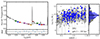 |
Fig. 8. Stellar mass estimations. Left: Spectral energy distribution (SED) for galaxy ID = 22 055 at z = 0.9856 from field J1039p0714. The black line represents the best fit template. The solid bars represent the pseudo-narrow bands. Right: Stellar-mass vs redshift for the galaxies in the DR2 catalogue at 0.35 < z < 1.5. The squares represent the galaxies within 500 km s−1 of the Mg II absorbers and with impact parameters b < 100 kpc. The histogram shows the normalised stellar mass distributions. |
5.2. Star formation rates
We compute dust-corrected SFRs using the [O II] fluxes using the procedure presented in Langan et al. (2023), which is based on the empirical calibration of Gilbank et al. (2010, 2011) that incorporates the dependence of the Balmer decrement with stellar mass. Specifically, we used
![Mathematical equation: $$ \begin{aligned} \mathrm{SFR}=\frac{\mathrm{L}_{[\mathrm{O}\,{ii }]}/(1.12\times 2.53\times 10^{40}\,\mathrm{erg\,s}^{-1})}{a\times \tanh [(x-b)/c]+d}, \end{aligned} $$](/articles/aa/full_html/2025/02/aa51093-24/aa51093-24-eq36.gif) (3)
(3)
where L[O II] is the [O II] luminosity, x = log M⋆, a, b, c = −1.424, 9.827, 0.572, and d = 1.70. The factor 1.12 converts the Gilbank et al. (2010) calibration to the Chabrier (2003) IMF used throughout the survey.
5.3. Morpho-kinematics
In order to derive the morpho-kinematic of the galaxies, we used the GALPAK3D algorithm (Bouché et al. 2015), which performs a forward fit of a disk model with 10 free parameters directly on the 3D MUSE data. GALPAK3D takes into account the effect of the spectral line spread function (LSF) and of the point spread function (PSF) to deconvolve the observations and yields the intrinsic galaxy properties. These include: the main axis orientation, inclination, half-light radius, maximum velocity, and velocity dispersion, along with the flux and the position of the galaxy. We ran GALPAK3D on subcubes centred on either [O II], [O III] or Hα emission lines, with the continuum subtracted, using the PSF from Sect. 3.1 and the LSF as in Bacon et al. (2023); namely, the median LSF FWHM is LSF[Å](λ) = 5.866 × 10⁻⁸λ2 − 9.187 × 10⁻⁴λ + 6.040, where λ is in Å.
6. Results
6.1. Matching galaxies with absorbers
The association of absorption systems with their galaxy counterparts is crucial to understanding the physical processes at play in the CGM. We first associated the galaxies to Mg II absorption lines according to the redshift difference between the galaxy and the absorption, Δv. Using a Δv = 500 km s−1, the number of galaxies (in the entire MUSE FOV) per Mg II absorption system was derived. From its distribution shown in Fig. 9 (left), we can see that there is approximately an average of
 (4)
(4)
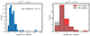 |
Fig. 9. Galaxies per absorption system. Left: Distribution of the number of galaxies that are within ±500 km s−1 of strong ( |


galaxies per absorber. As discussed in Cherrey et al. (2024), this is close to the expected mean number of galaxies, namely,
 (5)
(5)
in a cylinder of radius of rmax < 280 kpc, (corresponding to the same area of the MUSE FOV) and height of Δz = 500 km s−1 for galaxies in halos of mass Mh > 1011 M⊙ using the halo mass function from Tinker & Chen (2008). We note that the drop in Fig. 9 (left) at N = 5 is entirely caused by the MUSE FOV.
If we restrict ourself to galaxies within an impact parameter b less than 100 kpc, the red-filled histogram in Fig. 9 (right) shows the number of galaxies that are within b < 100 kpc around 80 strong ( Å) absorption systems. This figure shows that the majority (60 out of 80, i.e. 75%) of Mg II systems are matched with one or two galaxies, and only ten have no counterparts at all.
Figure 10 shows the velocity difference (Δv) between the galaxy redshift and the absorption redshift as a function of the impact parameter, b. The δv standard deviation is σ ∼ 100 km s−1, much smaller than our search boundary of ±500 km s−1, as in Huang et al. (2021). This shows that, in spite of our search range of |Δv|< 500 km s−1 (solid horizontal lines), the galaxies associated with the Mg II absorbers are found within ±200 km s−1 from the absorption lines and within ±100 km s−1 at distances less than 50 kpc. The dotted line represents the escape velocity, vesc of a 1012 (Navarro et al. 1997, NFW) halo; this figure indicates that the Mg II gas is not virialised, as Δv decreases towards the centre, whereas it would increase as in groups (Cherrey et al. 2024) if the gas were virialised. It shows also that we are not likely affected by mis-assigned gas, namely, within |Δv|< 500 km s−1 but outside the virial radius. This was discussed in Ho et al. (2020) in the context of the Mg II in EAGLE simulations or in Weng et al. (2024) in the context of Lyman limit systems in TNG50.
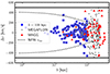 |
Fig. 10. Velocity offset Δv versus impact parameter b. The squares show the MEGAFLOW sample for galaxies within the impact parameter of b < 100 or b < 250 kpc. The triangles represent the MAGG sample from Dutta et al. (2020). The dotted line represents the escape velocity vesc for the median halo mass of isolated galaxies Mh = 1011.7 M⊙ (Cherrey et al. 2025). |
6.2. Comparison between DR1 and DR2 galaxy catalogues
A notable difference between our DR1 and DR2 galaxy catalogue is that the DR1 galaxy catalogue from Zabl et al. (2019) was constructed primarily from pseudo-narrow band images at the redshift of [O II] corresponding to the Mg II absorption catalogue, while the final DR2 catalogue is constructed in such a way that it is totally blind to the presence of Mg II absorptions.
Out of the 80 (69) systems in DR2 (DR1), there are 115 (80) galaxies within 100 kpc associated with absorbers in the DR2 (DR1) samples, respectively. This corresponds to a ‘success’ rate in finding at least one galaxy of ∼90% (see Table 7) for strong Mg II systems ( Å), compared to DR1 which had ≈80% success rate (Schroetter et al. 2019; Zabl et al. 2019).
Success rate in finding the host galaxy with [O II] within the MUSE wavelength coverage, i.e. at 0.35 < zabs < 1.5.
Fig. 9 (right) compares the number of galaxies per absorber within b < 100 kpc, for strong ( Å) Mg II systems. The red (grey) histogram represents the number of galaxies per absorption lines in the DR2 (DR1) catalogues. This figure also shows that there are fewer systems (10 vs 14) without galaxies, while there are more systems (80 vs 58) with one or two galaxies.
Figure 11 compares the properties of the DR2 and DR1 catalogues, in particular it compares the redshift, magnitude, and impact parameters of the galaxies associated with Mg II absorptions at 0.3 < z < 1.5 in the DR1 and DR2 catalogues. The difference between the red solid and hashed histogram shows the benefit from a blind approach.
 |
Fig. 11. Comparison between the DR2 and DR1 galaxy sample of galaxies within ±500 km s−1 around each Mg II absorption system and within 100 kpc. The left, middle, and right panels show the redshift, magnitude, and impact parameter distributions for galaxies in the redshift range 0.3 < zabs < 1.5, respectively. |
6.3. Primary galaxy
Within the MEGAFLOW sample, we define ‘primary’ galaxies as the ones we could unambiguously identify as responsible for Mg II absorption in quasar spectra (if any, at the same redshift). We identify these primary galaxies blindly (without considering Mg II absorptions) by applying the following criteria:
-
0.3 < z < 1.5;
-
ZCONF ≥ 2;
-
zgal < zQSO with ΔvQSO ≥ 1000 km s−1;
-
b < 150 kpc;
-
Smallest b within ±1000 km s−1. Any neighbor must have b at least 50 kpc greater;
-
NFOV < 5 to avoid groups.
Here, zgal and zQSO are, respectively, the redshift of the galaxy and the redshift of the quasar of the field, with ΔvQSO as the velocity difference between the quasar and the galaxy and NFOV being the number of galaxies in the MUSE field of view in a ±1000 km s−1 window. In total, 170 primary galaxies have been identified. Finally, out of the 115 absorptions in the redshift range 0.3 < z < 1.5, 43 can unambiguously be associated with a primary galaxy. On the other hand, 127 primary galaxies are not associated with any absorption.
This set of primary galaxies (associated or not associated with an absorption) are particularly useful in improving our understanding of the physical parameters responsible for the presence of an Mg IIλλ2796, 2803 absorption at a given impact parameter.
6.4. SFR distribution
We investigated the impact of the SFR on the presence of a counterpart Mg II absorption by comparing the SFR distribution for primary galaxies (as described in 6.1) associated with an absorption to those not associated with an absorption. Figure 12 shows the stellar mass versus SFR, namely the main sequence for these two sub-samples. We can see that this MUSE survey is sensitive to galaxies with M⋆ ≳ 107.5 and SFR ≳ 0.01 M⊙ yr−1, but that the majority of Mg II host galaxies have SFR > 1 M⊙ yr−1 and M⋆ > 109 M⊙. This indicates that the survey would have detected satellites with mass ratio 1 : 20 or greater.
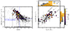 |
Fig. 12. Star formation rates. Left: Measured [O II] flux versus SDSS r magnitude recomputed with PHOTUTILS. The full MEGAFLOW sample is represented with gray dots. Colored and black dots represent, respectively, the primary galaxies that are associated and not associated with a counterpart absorption. Galaxies with no detected [O II] flux are represented by downward arrows. Right: Estimated stellar mass versus estimated SFR for the primary galaxies. The top and right histograms present respectively the stellar mass distribution and the SFR distribution for the galaxies associated (orange) and not associated (gray) with a Mg II absorption. Arrows on the left indicates galaxies without stellar mass estimation and/or no SFR estimation (because no [O II] emission detected). The primary galaxies associated with an absorption are colored according to the Mg II absorption rest-frame equivalent width. Error bars are 1σ uncertainties. |
6.5. Gas density profile
Figure 13 shows the REW impact parameter ( ) relation. The squares (circles) shows the relation for the primary galaxies with N100 = 1 (N100 > 1), respectively. In Cherrey et al. (2024), we investigate the
  relation for group-selected pairs and the associated in groups. In Cherrey et al. (2025), we investigate the
  relation for isolated galaxies, along with its dependence with respect to SFR, mass, redshift, and azimuthal angle, α.
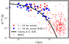 |
Fig. 13. REW ( |


6.6. Considering the effect of pre-selecting sight lines
The MEGAFLOW survey is inherently an absorption-centred survey with the pre-selection of sight lines with Mg II absorption lines (as discussed in Sect. 2). However, the wide wavelength range and, hence, the wide redshift coverage (0.3 < z < 1.5) allow us to perform a galaxy-centred analysis, that is aimed, for instance, at the characterisation of the covering fraction; namely, the fraction of galaxies that have a Mg II absorption above some column density or REW (Schroetter et al. 2021) or that of groups comprised of more than five galaxies (Cherrey et al. 2024). In Schroetter et al. (2021), we investigated the covering fraction of Mg II absorptions at 1.0 < z < 1.4, using a preliminary version of the MEGAFLOW galaxy catalogue. With the full DR2 catalogue in hand, we aim to revisit the Mg II covering fraction for galaxies across the full redshift range, 0.3 < z < 1.5, as a function of azimuthal angle and galaxy properties in a forthcoming paper (Cherrey et al. 2025). Here, we address the potential impact of the pre-selection of sight lines (Sect. 2).
Such a galaxy-centred analysis is, in fact, possible in MEGAFLOW for a number of reasons. First, each MUSE field has ≈50 galaxies at 0.3 < z < 1.5 observed over 2000 independent channels taking into account the spectral resolution; thus, the pre-selection of fields only affects 5–10% of the sample. Second, the shape of the REW distribution dn/dW in MEGAFLOW is consistent with that of field or random sight lines (as discussed in Sect. 4.1 and Fig. 4), also noted in Schroetter et al. (2021). We should note that if the pre-selection of sight lines would bias the results, the galaxy covering fractions in Schroetter et al. (2021) do not seem to be different from other surveys (e.g. Nielsen et al. 2013b; Lan 2020; Huang et al. 2021; Dutta et al. 2020).
Nonetheless, to further quantify the effect of our pre-selection, we performed the following experiment. We populated MUSE-like fields with galaxies, each with their own CGM (assumed to be a gas sphere). After applying a MEGAFLOW pre-selection, we can compute the covering fraction on these selected fields and compare it the covering fraction obtained using all fields (down to the same REW limit).
In particular, we generated 50 MUSE-like fields (500 × 500 pkpc in projected size corresponding to 1 × 1 arcmin) and drew 100 galaxies per field from a Poisson distribution across a redshift range (0.4 < z < 1.4). We assigned a stellar mass from log M = 9.5 to log M = 11.5 according to a power law distribution of −1.5. We then assigned a truncated sphere of gas around each galaxy (similar to Tinker & Chen 2008), with the gas density following a power law of ρ ∝ r−α with α ≈ 2 − 1.5, truncated at Rtr = 100 kpc. We set the normalisation of the density profile such that the column density reaches ∼1020 cm−2 at 10 kpc adding a mass dependence (∝0.3log M) following the observed relation (Chen et al. 2010a). We can then compute the line-of-sight column density for each intercepted sphere and transform it into a REW using the  relation from Ménard & Chelouche (2009). The resulting equivalent widht
  distribution is shown in Fig. 14 and is in good agreement with the observed distribution of strong absorbers (Nestor et al. 2005; Zhu & Ménard 2013).
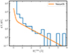 |
Fig. 14. Equivalent width distribution |

For each field, we computed the number of absorptions with a  greater than 0.6 Å, corresponding to pre-selection of strong Mg II absorbers. Using only the ∼9 − 10 fields, with 3 or more strong absorptions, mimicking the MEGAFLOW pre-selection, we computed the 2D covering fraction as a function of impact parameter and galaxy mass, fc(log b, log M) using the method used in Schroetter et al. (2021) and Cherrey et al. (2024). Using only the selected sight lines, the radius r50, radius at which fc(r50|log M = 10.5) is 50%, is then:
 (6)
(6)
When using all sight lines, this radius is:
 (7)
(7)
The mass dependence between  and r50 is found to be ∝(0.09 ± 0.03)log M for the selected sight lines and ∝(0.07 ± 0.02)log M for all sight lines.
Apart from the larger statistical uncertainty due to the smaller number of fields, the values are very consistent with each other, and we conclude that there is no inherent bias in covering fractions due to the MEGAFLOW pre-selection criteria. We refer to Cherrey et al. (2024) for similar arguments using different assumptions.
7. Discussion on [O II] versus continuum selected galaxies
The MEGAFLOW survey follows a dual galaxy identification process, based on continuum and emission lines (described in Sect. 4.2). This allows for the identification of line emitters ([O II], Lyα) without any continuum in the MUSE observations. In the final catalogue (DR2 v2.0) from the MUSE data, we find that 20% (30%) of galaxies with ZCONF ≥ 2 (≥1) do not have a continuum ID (WHITE_ID), respectively. For [O II] emitters at 0.3 < z < 1.5, the fraction is 8-15% depending on the redshift confidence ZCONF flag (see Table 8). For the low-redshift galaxies with ZCONF ≥ 2 that are within 100 kpc and 500 km s−1 of a Mg II absorption, 13 out of 138 were detected only from their emission lines. For the primary galaxies within 100 kpc, 5 out of 58 were detected only from their emission lines. Hence, 10% of galaxies at 0.3 < z < 1.5 have been detected only from their emission lines.
Galaxies without continuum or without FELINE detection.
However, not all sources without WHITE_ID are faint objects below the detection limit. Figure 15 shows the F775W ( ∼ i) magnitude distribution of these galaxies without WHITE_ID. At high redshifts (z > 2.8), the top panel reveals that almost all have i = 26 − 28 mag, namely, they are below the completeness limit. At low redshifts (z < 1.5), the bottom panel reveals a population of galaxies without WHITE_ID but with bright i < 26 mag, which can often be traced to failed deblending or to a bright foreground or background object contaminating the flux measurement. The green histogram shows the 13 galaxies with ZCONF ≥ 2 that are within 100 kpc and 500 km s−1 of Mg II absorptions, which are very relevant for the MEGAFLOW survey.
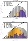 |
Fig. 15. Number counts for galaxies without continuum detection, without a WHITE_ID. The bottom (top) panel shows the distributions for low (high) redshift galaxies with 0.3 < z < 1.5 (2.8 < z < 6) respectively. Both panels show that there is a significant popultion of galaxies detected solely on their emission line with FELINE. The solid line represents the GAMMA/DEVILS survey (Koushan et al. 2021). |
The advantage of the dual detection method can be seen in Figure 12 (left), which shows the r-band magnitude versus the [O II] flux for the primary galaxies in MEGAFLOW with or without Mg II absorption. From this figure, we can see that the FELINE line detection allows us to detect object beyond the continuum limit of r ≃ 25 mag. Figure 16 shows two examples of galaxies with [O II] emission and no continuum.
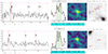 |
Fig. 16. Examples of [O II] emitters without continuum for source ID = 11 040 and ID = 25 036. More information available on the AMUSED interface. For each source, the MUSE spectra, [O II] emission, pseudo-narrow-band image at [O II], and the white-light continuum image are shown. |
Similarly, in the Muse eXtremely Deep Field [MXDF; 140 h] from Bacon et al. (2023), who performed also a dual continuum and emission line detection, there are 175 out of 886 Lyα emitters (20%) that have no counterparts in the HST catalogue (Rafelski et al. 2015) and 96 out 886 Lyα emitters (10%) have no detectable signal in the deep HST/UDF images. For comparison, the MAGG sample (Lofthouse et al. 2020) is based on continuum identification and does not include blind emission line galaxies. Similarly, the QSAGE sample (Bielby et al. 2019) is based on continuum identification on shallow 250s WFC3 F140W images. The sample from the MUSE Ultra Deep Field [MUDF; 150 h] of Fossati et al. (2019) and Revalski et al. (2023) used deep (6.5 h) continuum F140W images for their catalogue identification.
8. Conclusions
In this paper, we present the MEGAFLOW survey, a MUSE and UVES survey designed to better understand the CGM using low-ionisation metal Mg II lines in 22 QSO fields. We describe the survey strategy (Sect. 2) and detail the MUSE and UVES data (Sect. 3), along with the data products (4).
The MEGAFLOW survey targeted 22 QSO fields, with at least three Mg II absorptions lines, with rest-frame  Å, leading to 79 Mg II absorption lines. From the UVES spectra, we found additional Mg II absorption lines, leading to a total of 127 Mg II absorption lines. The rest-frame equivalent width distribution follows the expected power-law distribution of random sight lines, albeit with a boosted normalisation (Fig. 4).
Regarding this MUSE GTO programme, the observations taken between 2014 and 2019, cover 22 arcmin2, two fields (J0014−0028, J0937+0656) were observed at 10–11 h depths, while the other 20 fields were observed at 2–5 h depths. The 3σ sensitivity for emission lines at 7000 Å is typically 5 × 10⁻¹⁹ erg s−1 cm−2 arcsec−2 for the 10 h depth cubes, and 7.5 × 10⁻¹⁹ erg s−1 cm−2 arcsec−2 for the 3–4 h depth cubes. As discussed in Sect. 4.3, the 50% completeness limit for the 10 h (2.5 h) cubes is 3.7 erg s−1 cm−2 (7.07
 erg s−1 cm−2) [O II] emitters at ≈7000 Å, and is approximately i ∼ mF775W ≈ 26 mAB (25.2 mAB) for continuum sources, respectively.
The final catalogue (v2.0) from the MEGAFLOW survey contains 2427 sources, which includes 22 Quasars, 57 stars, 2020 galaxies with ZCONF ≥ 1 and 350 sources with no redshifts (ZCONF = 0). As discussed in Sect. 4.2, we use a dual galaxy identification process based both on continuum (using SExtractor; Bertin & Arnouts 1996) and on [O II] emission lines (using FELINE; Wendt et al. 2024). This approach is similar to the MUSE UDF analysis of Bacon et al. (2023). It has the significant advantage that [O II] emitters without continuum counterpart can be identified (Fig. 16). Overall, we find that one-third (718/1998) of galaxies with redshift flag ZCONF ≥ 1 have no continuum detection down to r ≈ 28.5 mAB. For [O II] emitters at 0.3 < z < 1.5, we find 8 (15) per cent of galaxies without a continuum detection for sources with ZCONF ≥ 2 (≥1) (Table 8).
For strong ( Å) Mg II absorbers in the redshift range 0.35 < z < 1.5, where [O II] can be identified in the MUSE wavelength coverage, the success rate of detecting the host galaxy within 100 kpc is 90% (Table 7). The mean number of galaxies per absorber is ∼3 within the MUSE FOV, while 40 (20) absorbers have one (two) galaxies within 100 kpc.
All but two of the host galaxies have SFR greater than 1 M⊙ yr−1 and stellar masses above 109 M⊙, after performing SED fitting on the MUSE data using 13 pseudo-medium filters. Given that this MUSE survey is sensitive to galaxies with M⋆ ≳ 107.5 and SFR ≳ 0.01 M⊙ yr−1 (Fig. 12), we can rule out the role of LMC-like satellites for strong Mg II systems with  Å. This is supported by the fact that we would have detected satellites with mass ratio 1 : 20 or greater in such cases.
Data availability
The MUSE and UVES raw data used for this article are available in the ESO archive13. The reduced MUSE data-cubes are available on the MuseWise website14 The MUSE and UVES products, the MEGAFLOW catalogues and MUSE advanced data products are also available on the AMUSED website15.
This filter width gives the optimal S/N for [O II] λλ3727,3729 doublet assuming a line width of FWHM ≈ 50 km s−1.
A python-inspired version of the PLATEFIT IDL code (Brinchmann et al. 2004).
Acknowledgments
This study is based on observations collected at the European Southern Observatory under ESO programmes listed in Tables 2 and 3. This work has been carried out thanks to the support of the ANR FOGHAR (ANR-13-BS05-0010), the ANR 3DGasFlows (ANR-17-CE31-0017), and the OCEVU Labex (ANR-11-LABX-0060). LW acknowledges funding by the European Research Council through ERC-AdG SPECMAP-CGM, GA 101020943. RB acknowledges support from the ANR L-INTENSE (ANR-CE92-0015). Software: This work makes use of the following open source software: GALPAK3D (Bouché et al. 2015), FELINE (Wendt et al. 2024), ZAP (Soto et al. 2016), MPDAF (Piqueras et al. 2019), MATPLOTLIB (Hunter 2007), NUMPY (Van Der Walt et al. 2011), ASTROPY (The Astropy Collaboration 2018), MAOPPY (Fétick et al. 2019), PAMPELMUSE (Kamann et al. 2013), PHOTUTILS (Bradley et al. 2022), DUSTMAPS (Green 2018), and PYMC3 (Salvatier et al. 2016).
References
- Abbas, A., Churchill, C. W., Kacprzak, G. G., et al. 2024, ApJ, 966, 242 [NASA ADS] [CrossRef] [Google Scholar]
- Amorisco, N. C., & Bertin, G. 2010, A&A, 519, A47 [NASA ADS] [CrossRef] [EDP Sciences] [Google Scholar]
- Bacon, R., Accardo, M., Adjali, L., et al. 2010, Society of Photo-Optical Instrumentation Engineers (SPIE) Conference Series, 8 [Google Scholar]
- Bacon, R., Conseil, S., Mary, D., et al. 2017, A&A, 608, A1 [NASA ADS] [CrossRef] [EDP Sciences] [Google Scholar]
- Bacon, R., Mary, D., Garel, T., et al. 2021, A&A, 647, A107 [NASA ADS] [CrossRef] [EDP Sciences] [Google Scholar]
- Bacon, R., Brinchmann, J., Conseil, S., et al. 2023, A&A, 670, A4 [NASA ADS] [CrossRef] [EDP Sciences] [Google Scholar]
- Bahcall, J. N., & Spitzer, Lyman J. 1969, ApJ, 156, L63 [NASA ADS] [CrossRef] [Google Scholar]
- Bergeron, J., & Boissé, P. 1991, A&A, 243, 344 [NASA ADS] [Google Scholar]
- Bergeron, J., Cristiani, S., & Shaver, P. A. 1992, A&A, 257, 417 [NASA ADS] [Google Scholar]
- Bergeron, J., Petitjean, P., Sargent, W. L. W., et al. 1994, ApJ, 436, 33 [NASA ADS] [CrossRef] [Google Scholar]
- Bertin, E., & Arnouts, S. 1996, A&AS, 117, 393 [NASA ADS] [CrossRef] [EDP Sciences] [Google Scholar]
- Bielby, R., Crighton, N. H. M., Fumagalli, M., et al. 2017, MNRAS, 468, 1373 [CrossRef] [Google Scholar]
- Bielby, R. M., Stott, J. P., Cullen, F., et al. 2019, MNRAS, 486, 21 [CrossRef] [Google Scholar]
- Bouché, N. F., & McConway, K. 2019, Bioelectromagnetics, 40, 539 [CrossRef] [Google Scholar]
- Bouché, N. F., Murphy, M. T., Péroux, C., Csabai, I., & Wild, V. 2006, MNRAS, 371, 495 [CrossRef] [Google Scholar]
- Bouché, N. F., Murphy, M. T., Péroux, C., et al. 2007, ApJ, 669, L5 [CrossRef] [Google Scholar]
- Bouché, N. F., Carfantan, H., Schroetter, I., Michel-Dansac, L., & Contini, T. 2015, AJ, 150, 92 [CrossRef] [Google Scholar]
- Bradley, L., Sipocz, B., Robitaille, T., et al. 2022, https://doi.org/10.5281/zenodo.6825092 [Google Scholar]
- Brinchmann, J., Charlot, S., White, S. D. M., et al. 2004, MNRAS, 351, 1151 [Google Scholar]
- Bruzual, G., & Charlot, S. 2003, MNRAS, 344, 1000 [NASA ADS] [CrossRef] [Google Scholar]
- Calzetti, D., Armus, L., Bohlin, R. C., et al. 2000, ApJ, 533, 682 [NASA ADS] [CrossRef] [Google Scholar]
- Cardelli, J. A., Clayton, G. C., & Mathis, J. S. 1989, ApJ, 345, 245 [Google Scholar]
- Chabrier, G. 2003, PASP, 115, 763 [Google Scholar]
- Chen, H.-W., & Tinker, J. L. 2008, ApJ, 687, 745 [NASA ADS] [CrossRef] [Google Scholar]
- Chen, H.-W., Helsby, J. E., Gauthier, J.-R., et al. 2010a, ApJ, 714, 1521 [NASA ADS] [CrossRef] [Google Scholar]
- Chen, H., Wild, V., Tinker, J. L., et al. 2010b, ApJ, 724, L176 [NASA ADS] [CrossRef] [Google Scholar]
- Chen, H.-W., Zahedy, F. S., Boettcher, E., et al. 2020, MNRAS, 497, 498 [NASA ADS] [CrossRef] [Google Scholar]
- Cherrey, M., Bouché, N. F., Zabl, J., et al. 2024, MNRAS, 528, 481 [NASA ADS] [CrossRef] [Google Scholar]
- Cherrey, M., Bouché, N. F., Zabl, J., et al. 2025, A&A, in press, https://doi.org/10.1051/0004-6361/202451165 [NASA ADS] [CrossRef] [EDP Sciences] [Google Scholar]
- Churchill, C. W., Trujillo-Gomez, S., Nielsen, N. M., & Kacprzak, G. G. 2013, ApJ, 779, 87 [NASA ADS] [CrossRef] [Google Scholar]
- DeFelippis, D., Bouché, N. F., Genel, S., et al. 2021, ApJ, 923, 56 [NASA ADS] [CrossRef] [Google Scholar]
- Dekker, H., D’Odorico, S., Kaufer, A., Delabre, B., & Kotzlowski, H. 2000, in Proc. SPIE, eds. M. Iye, & A. F. Moorwood, Optical and IR Telescope Instrumentation and Detectors, 4008, 534 [NASA ADS] [CrossRef] [Google Scholar]
- Dutta, R., Fumagalli, M., Fossati, M., et al. 2020, MNRAS, 499, 5022 [CrossRef] [Google Scholar]
- Eisenhauer, F., Abuter, R., Bickert, K., et al. 2003, in Proceedings of the SPIE, eds. M. Iye, & A. F. M. Moorwood, Instrument Design and Performance for Optical/Infrared Ground-based Telescopes, 4841, 1548 [NASA ADS] [CrossRef] [Google Scholar]
- Fétick, R. J. L., Fusco, T., Neichel, B., et al. 2019, A&A, 628, A99 [NASA ADS] [CrossRef] [EDP Sciences] [Google Scholar]
- Fossati, M., Fumagalli, M., Lofthouse, E. K., et al. 2019, MNRAS, 490, 1451 [NASA ADS] [CrossRef] [Google Scholar]
- Freundlich, J., Bouché, N. F., Contini, T., et al. 2021, MNRAS, 501, 1900 [NASA ADS] [Google Scholar]
- Fumagalli, M., Prochaska, J. X., Kasen, D., et al. 2011, MNRAS, 418, 1796 [CrossRef] [Google Scholar]
- Gauthier, J.-R. 2013, MNRAS, 432, 1444 [NASA ADS] [CrossRef] [Google Scholar]
- Gauthier, J., Chen, H., & Tinker, J. L. 2009, ApJ, 702, 50 [NASA ADS] [CrossRef] [Google Scholar]
- Gilbank, D. G., Baldry, I. K., Balogh, M. L., Glazebrook, K., & Bower, R. G. 2010, MNRAS, 405, 2594 [NASA ADS] [Google Scholar]
- Gilbank, D. G., Baldry, I. K., Balogh, M. L., Glazebrook, K., & Bower, R. G. 2011, MNRAS, 412, 2111 [NASA ADS] [CrossRef] [Google Scholar]
- Green, G. 2018, J. Open Source Softw., 3, 695 [NASA ADS] [CrossRef] [Google Scholar]
- Herenz, E. C., & Wisotzki, L. 2017, A&A, 602, A111 [NASA ADS] [CrossRef] [EDP Sciences] [Google Scholar]
- Hinton, S. R., Davis, T. M., Lidman, C., Glazebrook, K., & Lewis, G. F. 2016, Astron. Comput., 15, 61 [Google Scholar]
- Ho, S. H., Martin, C. L., & Turner, M. L. 2019, ApJ, 875, 54 [NASA ADS] [CrossRef] [Google Scholar]
- Ho, S. H., Martin, C. L., & Schaye, J. 2020, ApJ, 904, 76 [NASA ADS] [CrossRef] [Google Scholar]
- Hoffman, M. D., & Gelman, A. 2014, J. Mach. Learn. Res., 15, 1593 [Google Scholar]
- Huang, Y.-H., Chen, H.-W., Shectman, S. A., et al. 2021, MNRAS, 502, 4743 [NASA ADS] [CrossRef] [Google Scholar]
- Hunter, J. D. 2007, Comput. Sci. Eng., 9, 90 [NASA ADS] [CrossRef] [Google Scholar]
- Kacprzak, G. G., Murphy, M. T., & Churchill, C. W. 2010, MNRAS, 406, 445 [NASA ADS] [CrossRef] [Google Scholar]
- Kacprzak, G. G., Churchill, C. W., Barton, E. J., & Cooke, J. 2011, ApJ, 733, 105 [NASA ADS] [CrossRef] [Google Scholar]
- Kamann, S., Wisotzki, L., & Roth, M. M. 2013, A&A, 549, A71 [NASA ADS] [CrossRef] [EDP Sciences] [Google Scholar]
- Kimm, T., Slyz, A., Devriendt, J., & Pichon, C. 2011, MNRAS, 413, L51 [Google Scholar]
- Koushan, S., Driver, S. P., Bellstedt, S., et al. 2021, MNRAS, 503, 2033 [NASA ADS] [CrossRef] [Google Scholar]
- Lan, T.-W. 2020, ApJ, 897, 97 [NASA ADS] [CrossRef] [Google Scholar]
- Langan, I., Zabl, J., Bouché, N. F., et al. 2023, MNRAS, 521, 546 [NASA ADS] [CrossRef] [Google Scholar]
- Lanzetta, K. M., & Bowen, D. 1990, ApJ, 357, 321 [NASA ADS] [CrossRef] [Google Scholar]
- Lofthouse, E. K., Fumagalli, M., Fossati, M., et al. 2020, MNRAS, 491, 2057 [NASA ADS] [CrossRef] [Google Scholar]
- Lundgren, B. F., Brunner, R. J., York, D. G., et al. 2009, ApJ, 698, 819 [NASA ADS] [CrossRef] [Google Scholar]
- Lundgren, B. F., Creech, S., Brammer, G., et al. 2021, ApJ, 913, 50 [NASA ADS] [CrossRef] [Google Scholar]
- Mary, D., Bacon, R., Conseil, S., Piqueras, L., & Schutz, A. 2020, A&A, 635, A194 [EDP Sciences] [Google Scholar]
- Ménard, B., & Chelouche, D. 2009, MNRAS, 393, 808 [CrossRef] [Google Scholar]
- Mishra, S., & Muzahid, S. 2022, ApJ, 933, 229 [NASA ADS] [CrossRef] [Google Scholar]
- Murphy, M. 2018, https://doi.org/10.5281/zenodo.1297190 [Google Scholar]
- Murphy, M. T., Kacprzak, G. G., Savorgnan, G. A. D., & Carswell, R. F. 2019, MNRAS, 482, 3458 [NASA ADS] [CrossRef] [Google Scholar]
- Muzahid, S., Schaye, J., Marino, R. A., et al. 2020, MNRAS, 496, 1013 [Google Scholar]
- Navarro, J. F., Frenk, C. S., & White, S. D. M. 1997, ApJ, 490, 493 [Google Scholar]
- Nestor, D. B., Turnshek, D. A., & Rao, S. M. 2005, ApJ, 628, 637 [NASA ADS] [CrossRef] [Google Scholar]
- Nestor, D. B., Johnson, B. D., Wild, V., et al. 2011, MNRAS, 412, 1559 [NASA ADS] [CrossRef] [Google Scholar]
- Nielsen, N. M., Churchill, C. W., Kacprzak, G. G., & Murphy, M. T. 2013a, ApJ, 776, 114 [NASA ADS] [CrossRef] [Google Scholar]
- Nielsen, N. M., Churchill, C. W., & Kacprzak, G. G. 2013b, ApJ, 776, 115 [NASA ADS] [CrossRef] [Google Scholar]
- Ono, Y., Ouchi, M., Mobasher, B., et al. 2012, ApJ, 744, 83 [Google Scholar]
- Péroux, C., & Howk, J. C. 2020, ARA&A, 58, 363 [CrossRef] [Google Scholar]
- Péroux, C., Zwaan, M. A., Klitsch, A., et al. 2019, MNRAS, 485, 1595 [CrossRef] [Google Scholar]
- Pichon, C., Pogosyan, D., Kimm, T., et al. 2011, MNRAS, 418, 2493 [CrossRef] [Google Scholar]
- Piqueras, L., Conseil, S., Shepherd, M., et al. 2019, in Astronomical Data Analysis Software and Systems XXVI, Astronomical Society of the Pacific Conference Series, eds. M. Molinaro, K. Shortridge, & F. Pasian, 521, 545 [NASA ADS] [Google Scholar]
- Planck Collaboration XI. 2014, A&A, 571, A11 [NASA ADS] [CrossRef] [EDP Sciences] [Google Scholar]
- Planck Collaboration XIII. 2016, A&A, 594, A13 [NASA ADS] [CrossRef] [EDP Sciences] [Google Scholar]
- Rafelski, M., Teplitz, H. I., Gardner, J. P., et al. 2015, AJ, 150, 31 [Google Scholar]
- Revalski, M., Rafelski, M., Fumagalli, M., et al. 2023, ApJS, 265, 40 [NASA ADS] [CrossRef] [Google Scholar]
- Salvatier, J., Wiecki, T. V., & Fonnesbeck, C. 2016, PeerJ Comput. Sci., 2 [Google Scholar]
- Schaerer, D., & de Barros, S. 2009, A&A, 502, 423 [NASA ADS] [CrossRef] [EDP Sciences] [Google Scholar]
- Schroetter, I., Bouché, N., Wendt, M., et al. 2016, ApJ, 833, 39 [NASA ADS] [CrossRef] [Google Scholar]
- Schroetter, I., Bouché, N. F., Zabl, J., et al. 2019, MNRAS, 490, 4368 [CrossRef] [Google Scholar]
- Schroetter, I., Bouché, N. F., Zabl, J., et al. 2021, MNRAS, 506, 1355 [NASA ADS] [CrossRef] [Google Scholar]
- Schroetter, I., Bouché, N. F., Zabl, J., et al. 2024, A&A, 687, 39 [Google Scholar]
- Shen, S., Madau, P., Guedes, J., et al. 2013, ApJ, 765, 89 [NASA ADS] [CrossRef] [Google Scholar]
- Soto, K. T., Lilly, S. J., Bacon, R., Richard, J., & Conseil, S. 2016, MNRAS, 458, 3210 [Google Scholar]
- Spitzer, L., Jr. 1956, ApJ, 124, 20 [NASA ADS] [CrossRef] [Google Scholar]
- Steidel, C. C. 1993, in The Environment and Evolution of Galaxies, eds. J. M. Shull, & H. A. Thronson (Dordrecht: Kluwer), 263 [NASA ADS] [CrossRef] [Google Scholar]
- Steidel, C. C. 1995, in QSO Absorption Lines. ESO Astrophysics Symposia, ed. G. Meylan (Berlin, Germany: Springer-Verlag), 139 [CrossRef] [Google Scholar]
- Steidel, C. C., Dickinson, M., & Persson, S. E. 1994, ApJ, 437, L75 [NASA ADS] [CrossRef] [Google Scholar]
- Steidel, C. C., Bowen, D. V., Blades, J. C., & Dickinson, M. 1995, ApJ, 440, L45 [NASA ADS] [CrossRef] [Google Scholar]
- Steidel, C. C., Dickinson, M., Meyer, D. M., Adelberger, K. L., & Sembach, K. R. 1997, ApJ, 480, 568 [NASA ADS] [CrossRef] [Google Scholar]
- Steidel, C. C., Kollmeier, J. A., Shapley, A. E., et al. 2002, ApJ, 570, 526 [NASA ADS] [CrossRef] [Google Scholar]
- The Astropy Collaboration (Price-Whelan, A. M., et al.) 2018, AJ, 156, 123 [Google Scholar]
- Tinker, J. L., & Chen, H.-W. 2008, ApJ, 679, 1218 [NASA ADS] [CrossRef] [Google Scholar]
- Tumlinson, J., Peeples, M. S., & Werk, J. K. 2017, ARA&A, 55, 389 [Google Scholar]
- Valentijn, E. A., Begeman, K., Belikov, A., et al. 2017, in Astroinformatics, eds. M. Brescia, S. G. Djorgovski, E. D. Feigelson, G. Longo, & S. Cavuoti, 325, 333 [NASA ADS] [Google Scholar]
- Van Der Walt, S., Colbert, S. C., & Varoquaux, G. 2011, Comput. Sci. Eng., 13, 22 [Google Scholar]
- Weilbacher, P. M., Streicher, O., Urrutia, T., et al. 2014, in Astronomical Data Analysis Software and Systems XXIII, Astronomical Society of the Pacific Conference Series, eds. N. Manset, & P. Forshay, 485, 451 [NASA ADS] [Google Scholar]
- Weilbacher, P. M., Palsa, R., Streicher, O., et al. 2020, A&A, 641, A28 [NASA ADS] [CrossRef] [EDP Sciences] [Google Scholar]
- Wendt, M., Bouché, N. F., Zabl, J., Schroetter, I., & Muzahid, S. 2021, MNRAS, 502, 3733 [NASA ADS] [CrossRef] [Google Scholar]
- Wendt, M., Henschel, M., Soth, O. F., et al. 2024, JOSS, submitted [Google Scholar]
- Weng, S., Péroux, C., Ramesh, R., et al. 2024, MNRAS, 527, 3494 [Google Scholar]
- York, D. G., Adelman, J., Anderson, J. E., Jr., et al. 2000, AJ, 120, 1579 [NASA ADS] [CrossRef] [Google Scholar]
- Zabl, J., Freudling, W., Møller, P., et al. 2016, A&A, 590, A66 [NASA ADS] [CrossRef] [EDP Sciences] [Google Scholar]
- Zabl, J., Bouché, N. F., Schroetter, I., et al. 2019, MNRAS, 485, 1961 [NASA ADS] [CrossRef] [Google Scholar]
- Zabl, J., Bouché, N. F., Schroetter, I., et al. 2020, MNRAS, 492, 4576 [NASA ADS] [CrossRef] [Google Scholar]
- Zabl, J., Bouché, N. F., Wisotzki, L., et al. 2021, MNRAS, 507, 4294 [NASA ADS] [CrossRef] [Google Scholar]
- Zhu, G., & Ménard, B. 2013, ApJ, 770, 130 [NASA ADS] [CrossRef] [Google Scholar]
Appendix A: UVES EW limits
Figure A.1 shows the rest-frame  limits (3σ) for each field used in Fig. 3 as a function of redshifts which ranges from 0.05 to 0.1Å.
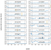 |
Fig. A.1. Rest-frame |

Appendix B: Description of the catalogues and products
Table B.1 describes the content of the galaxy catalogue. Table B.2 describes the content of the Mg II absorption catalogue. Table B.3 describes the available MUSE datasets and associated files. Figure B.1 shows an example of an html file displaying the summary information of each sources, available on the AMUSED interface.
Column description of the main galaxy catalog.
Column description of the Mg II absorption catalogue
List of MUSE datasets and associated files
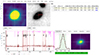 |
Fig. B.1. Example of a html file summarising the information regarding each source available from the AMUSED web interface. This source is the z = 0.702 galaxy ID 21113 with a Mg II halo presented in Zabl et al. (2021). |
All Tables
Magnitude (F775W) completeness limit (mAB) for the deep (shallow) fields, respectively.
Success rate in finding the host galaxy with [O II] within the MUSE wavelength coverage, i.e. at 0.35 < zabs < 1.5.
All Figures
|
Fig. 1. Schematic diagram of the steps in the data reduction process. |
| In the text | |
|
Fig. 2. White-light images (variance weighted) for the field J0014p0912 from different data-reductions. Left: Automatic data reduction from ESO. Middle: Data reduction (‘DR1’) using custom scripts as in Zabl et al. (2019). Right: Final data reduction (‘DR2’) used here using super flats (Sect. 3). |
| In the text | |
|
Fig. 3. Median 3σ REW limits for Mg II 2796 as a function of redshift for all 22 UVES spectra (solid black line). The blue and grey lines represent the 25th and 75th percentiles, respectively. Figure A.1 shows the REW limits for each field individually. The bottom graph shows the number of sight lines covering each redshift. |
| In the text | |
|
Fig. 4. Properties of the Mg II absorption catalogue. Top: Redshift distribution of the Mg II absorption systems. The solid and gray histograms show the absorbers for the SDSS (DR1) and UVES (DR2) selections, respectively. Bottom: Rest-frame equivalent width |
| In the text | |
|
Fig. 5. Completeness for [O II] emitters in the deep cube J0937+0656. (a) Completeness level (50%) as a function of redshifts. (b) Completeness as a function of size Re (top panel) and [O II] fluxes (bottom panel). The red (blue) squares represent the [O II] emitters detected (not detected), respectively. The shaded area represents the fit to the unbinned data. |
| In the text | |
|
Fig. 6. Magnitude distributions for the DR2 catalogue. Left: Magnitude F775W number counts. The grey histogram represents the entire MEGAFLOW survey. The magenta histogram represents the 20 shallow fields and the green histogram the 2 deep fields. Compared to the number counts from the GAMMA/DEVILS survey (solid line) from Koushan et al. (2021), the MEGAFLOW survey is 50%-complete to i ≈ 25.2 mAB (26 mAB) in the shallow (deep) fields, respectively. Right: Magnitude-redshift distribution of all sources with redshifts z > 0. The QSOs are shown as grey circles. The galaxies with ZCONF = 1 (2,3) are represented as green circles (blue squares), respectively. |
| In the text | |
|
Fig. 7. Schematic illustration of the process used to generate the final catalogue from the FELINE and continuum-based catalogues. |
| In the text | |
|
Fig. 8. Stellar mass estimations. Left: Spectral energy distribution (SED) for galaxy ID = 22 055 at z = 0.9856 from field J1039p0714. The black line represents the best fit template. The solid bars represent the pseudo-narrow bands. Right: Stellar-mass vs redshift for the galaxies in the DR2 catalogue at 0.35 < z < 1.5. The squares represent the galaxies within 500 km s−1 of the Mg II absorbers and with impact parameters b < 100 kpc. The histogram shows the normalised stellar mass distributions. |
| In the text | |
|
Fig. 9. Galaxies per absorption system. Left: Distribution of the number of galaxies that are within ±500 km s−1 of strong ( |
| In the text | |
|
Fig. 10. Velocity offset Δv versus impact parameter b. The squares show the MEGAFLOW sample for galaxies within the impact parameter of b < 100 or b < 250 kpc. The triangles represent the MAGG sample from Dutta et al. (2020). The dotted line represents the escape velocity vesc for the median halo mass of isolated galaxies Mh = 1011.7 M⊙ (Cherrey et al. 2025). |
| In the text | |
|
Fig. 11. Comparison between the DR2 and DR1 galaxy sample of galaxies within ±500 km s−1 around each Mg II absorption system and within 100 kpc. The left, middle, and right panels show the redshift, magnitude, and impact parameter distributions for galaxies in the redshift range 0.3 < zabs < 1.5, respectively. |
| In the text | |
|
Fig. 12. Star formation rates. Left: Measured [O II] flux versus SDSS r magnitude recomputed with PHOTUTILS. The full MEGAFLOW sample is represented with gray dots. Colored and black dots represent, respectively, the primary galaxies that are associated and not associated with a counterpart absorption. Galaxies with no detected [O II] flux are represented by downward arrows. Right: Estimated stellar mass versus estimated SFR for the primary galaxies. The top and right histograms present respectively the stellar mass distribution and the SFR distribution for the galaxies associated (orange) and not associated (gray) with a Mg II absorption. Arrows on the left indicates galaxies without stellar mass estimation and/or no SFR estimation (because no [O II] emission detected). The primary galaxies associated with an absorption are colored according to the Mg II absorption rest-frame equivalent width. Error bars are 1σ uncertainties. |
| In the text | |
|
Fig. 13. REW ( |
| In the text | |
|
Fig. 14. Equivalent width distribution |
| In the text | |
|
Fig. 15. Number counts for galaxies without continuum detection, without a WHITE_ID. The bottom (top) panel shows the distributions for low (high) redshift galaxies with 0.3 < z < 1.5 (2.8 < z < 6) respectively. Both panels show that there is a significant popultion of galaxies detected solely on their emission line with FELINE. The solid line represents the GAMMA/DEVILS survey (Koushan et al. 2021). |
| In the text | |
|
Fig. 16. Examples of [O II] emitters without continuum for source ID = 11 040 and ID = 25 036. More information available on the AMUSED interface. For each source, the MUSE spectra, [O II] emission, pseudo-narrow-band image at [O II], and the white-light continuum image are shown. |
| In the text | |
|
Fig. A.1. Rest-frame |
| In the text | |
|
Fig. B.1. Example of a html file summarising the information regarding each source available from the AMUSED web interface. This source is the z = 0.702 galaxy ID 21113 with a Mg II halo presented in Zabl et al. (2021). |
| In the text | |
Current usage metrics show cumulative count of Article Views (full-text article views including HTML views, PDF and ePub downloads, according to the available data) and Abstracts Views on Vision4Press platform.
Data correspond to usage on the plateform after 2015. The current usage metrics is available 48-96 hours after online publication and is updated daily on week days.
Initial download of the metrics may take a while.