| Issue |
A&A
Volume 694, February 2025
|
|
|---|---|---|
| Article Number | A117 | |
| Number of page(s) | 14 | |
| Section | Extragalactic astronomy | |
| DOI | https://doi.org/10.1051/0004-6361/202451165 | |
| Published online | 10 February 2025 | |
MusE GAs FLOw and Wind (MEGAFLOW)
XIII. Cool gas traced by Mg II around isolated galaxies
1
Univ Lyon1, Ens de Lyon, CNRS, Centre de Recherche Astrophysique de Lyon (CRAL) UMR5574, F-69230 Saint- Genis-Laval, France
2
Institute for Computational Astrophysics and Department of Astronomy & Physics, Saint Mary’s University, 923 Robie Street, Halifax, Nova Scotia B3H 3C3, Canada
3
Institut de Recherche en Astrophysique et Planétologie, Université de Toulouse, Centre National de la Recherche Scientifique, Centre National d’Etudes Spatiales, 31028 Toulouse, France
4
Institut für Physik und Astronomie, Universität Potsdam, Karl-Liebknecht-Str. 24/25, 14476 Potsdam, Germany
5
Centro de Astrobiologia (CAB), CSIC-INTA, Carretera de Ajalvir km 4, Torrejon de Ardoz, 28850 Madrid, Spain
6
Leiden Observatory, Leiden University, P.O. Box 9513 NL-2300 AA Leiden, The Netherlands
7
Leibniz-Institut for Astrophysik Potsdam (AIP), An der Sternwarte 16, 14482 Potsdam, Germany
⋆ Corresponding author; This email address is being protected from spambots. You need JavaScript enabled to view it.
Received:
18
June
2024
Accepted:
28
November
2024
Abstract
Aims. The circumgalactic medium (CGM) is a key component in understanding the physical processes governing the flows of gas around galaxies. Quantifying its evolution and its dependence on galaxy properties is particularly important for our understanding of accretion and feedback mechanisms.
Methods. We selected a volume-selected sample of 66 isolated star-forming galaxies at 0.4 < z < 1.5 with log(M⋆/M⊙) > 9 from the MusE GAs FLOw and Wind (MEGAFLOW) survey. Using Mg IIλλ2796,2803 absorptions in background quasars, we measured the covering fraction, fc, and quantified how the cool gas profile depends on galaxy properties (such as star formation rate (SFR), stellar mass (M⋆) or azimuthal angle relative to the line of sight) and how these dependencies evolve with redshift.
Results. The Mg II covering fraction of isolated galaxies is a strong function of impact parameter and is steeper than previously reported. The impact parameter, b50, at which fc = 50% is b50 = 50 ± 7 kpc for Wr2796 > 0.5 Å. It is weakly correlated with SFR (∝SFR0.08 ± 0.09) and decreases with cosmic time (∝(1 + z)0.8 ± 0.7), contrary to the expectation of increasingly larger halos with time. The covering fraction is also higher along the minor axis than along the major axis at the ≈2σ level.
Conclusions. The CGM traced by Mg II is similar across the isolated galaxy population. Indeed, among the isolated galaxies with an impact parameter below 55 kpc, all have associated Mg II absorption with Wr2796 > 0.3 Å, resulting in a steep covering fraction, fc(b).
Key words: galaxies: evolution / galaxies: halos / quasars: absorption lines
© The Authors 2025
 Open Access article, published by EDP Sciences, under the terms of the Creative Commons Attribution License (https://creativecommons.org/licenses/by/4.0), which permits unrestricted use, distribution, and reproduction in any medium, provided the original work is properly cited.
This article is published in open access under the Subscribe to Open model. This email address is being protected from spambots. You need JavaScript enabled to view it. to support open access publication.
1. Introduction
The circumgalactic medium (CGM) is a crucial element in understanding the formation and evolution of galaxies, as it constitutes an important reservoir of baryonic matter. It is a complex multiphase medium governed by multiple physical processes (Faucher-Giguère & Oh 2023). Observation of the diffuse gas in emission is challenging and requires focusing on resonant lines such as Lyα (e.g. Wisotzki et al. 2018) and/or using stacking techniques and deep observations (e.g., Zhang et al. 2016; Guo et al. 2023). Consequently, the CGM is often studied in absorption by searching for specific lines in bright background sources such as quasars. In particular, the Mg II absorption doublet λλ2796,2803 is known to be a good tracer of H I because of its low ionization potential. It is used to study the cool phase at ≈104 K (Bergeron & Stasińska 1986; Bergeron & Boissé 1991). Theory and observations seem to indicate that this phase is clumpy, with a volume filling factor of ≲1% and sub-kiloparsec clouds (Ménard & Chelouche 2009; Lan & Fukugita 2017; Faerman & Werk 2023; Hummels et al. 2024; Afruni et al. 2023). The Mg II doublet has the advantage of being accessible in the optical from ground-based telescopes at intermediate redshifts of 0.3 ≲ z ≲ 1.8, where the cosmic star formation is at its peak.
Several studies have shown how Mg II absorption equivalent width decreases as a function of the impact parameter, b, to the line of sight (Steidel et al. 1995; Bordoloi et al. 2011; Kacprzak et al. 2013; Nielsen et al. 2013a; Rubin et al. 2014; Schroetter et al. 2019; Lan 2020; Dutta et al. 2020, 2021; Huang et al. 2021; Lundgren et al. 2021). The Mg II-b anticorrelation extends to ≈50 to 150 kpc, with a large amount of scatter. This scatter can be explained first by the natural variations among the galaxy populations and second by the orientation and inclination of the galaxy relative to the line of sight, as outflows are preferentially ejected perpendicular to the galactic plane and accretion is more likely to happen in the galactic plane (Chen et al. 2010a; Kacprzak et al. 2012; Ho et al. 2017, 2019; Zabl et al. 2019; Schroetter et al. 2019; Péroux et al. 2020; Beckett et al. 2021; Nateghi et al. 2024a,b; Das et al. 2024).
An additional source of scatter can be the presence of neighbors close to the line of sight due to the natural spatial correlation of galaxies. Indeed, in quasar absorption studies, multiple galaxies are often detected at the absorption redshift within impact parameters of 100 kpc, making the pairing between galaxies and absorptions difficult. The solution is often to assume that the absorption is caused by the closest or the brightest galaxy. This approach is convenient but may be inaccurate. In addition, some neighbors may remain undetected due to completeness issues or a finite field of view. The presence of neighbors (detected or undetected) is problematic if we aim to measure the cool CGM profile, because the “superposed” contributions (Bordoloi et al. 2011; Nielsen et al. 2018) from individual galaxies increase the absorption strength.
In order to avoid this source of confusion we selected from the MusE GAs FLOw and Wind (MEGAFLOW) survey (presented in Sect. 2) a mass-complete sample of isolated galaxies (defined in Sect. 3), for which we determined the morphology and kinematics using the forward Bayesian modeling algorithm GalPaK3D (Sect. 4). We quantified in detail the cool gas profile and the Mg II covering fraction for this sample, and investigated how they are impacted by galaxy properties (Sect. 5).
Throughout, we used a standard flat ΛCDM cosmology with H0 = 69.3 km s−1 Mpc−1, ΩM = 0.29, and ΩΛ = 0.71 (see Hinshaw et al. 2013), with all distances given in proper kiloparsecs.
2. Data: The MEGAFLOW survey
The MEGAFLOW sample is based on the combination of integral field unit (IFU) data from the Very Large Telescope (VLT) Multi Unit Spectrograph Explorer (MUSE; Bacon et al. 2010) and Ultraviolet and Visible Echelle Spectrograph (UVES; Dekker et al. 2000) observations of 22 quasar fields. MUSE provides spectral cubes from which galaxies can be detected either from their continuum or from their emission lines (even without a continuum) over a large field of view of 1 × 1 arcmin2. Depending on the field, the exposure time spans from 1.7 hr (shallow field) to 11.2 hr (deep field), with a mean value of 3.9 hr. The PSF at 7000 Å is typically ≈0.7 arcsec. As discussed in Bouché et al. (2025), the galaxy sample is 50% complete down to i ≈ 25.2 mAB (26.0 mAB) for continuum-detected galaxies in the shallow (deep) fields, and ≈3.7 × 10⁻¹⁸ erg s−1 cm−2 (7 × 10⁻¹⁸ erg s−1 cm−2) for galaxies detected from their [O II] emission.
While the survey is designed around 79 strong Mg II absorption systems (rest-frame equivalent width  > 0.5 Å) selected from the Sloan Digital Sky Survey (SDSS) catalog of Zhu & Ménard (2013), additional Mg II absorptions have been identified in high-resolution UVES spectra down to ≈0.05 Å(3σ). The final Mg II catalog is composed of 127 Mg II absorption systems identified in the UVES spectra. Most of these (120) have a redshift of 0.3 < z < 1.5, for which the [O II] doublet falls in the MUSE range.
In this work, we use the galaxy catalog of the MEGAFLOW catalog (v2.0 beta) from Bouché et al. (2025) which contains a total of 1998 galaxies with redshifts. Among these galaxies, 730 have been identified solely from their emission lines (no continuum) and 1208 are located in the foreground of the 22 quasars. For more details about the MEGAFLOW survey catalog see Bouché et al. (2025).
3. Galaxy sample
In the present work, we quantified the Mg II profile around galaxies and measured its dependence on several galaxy properties such as star formation rate (SFR), z, and orientation. For this, we wanted to be sure that our absorption-galaxy pairing was unambiguous and we therefore focused on isolated galaxies with a redshift difference relative to the quasar corresponding to a velocity difference  . Isolated galaxies can be unambiguously associated with absorption (if present) and are unlikely to have experienced a major interaction in their recent history. We describe below the selection of our sample and the criteria we used to define “isolated” galaxies.
First, we selected galaxies in 0.4 < z < 1.5. In this redshift range, Mg II absorptions can be detected with UVES and galaxies can be detected from [O II] with MUSE. We only kept galaxies with a redshift confidence ZCONF ≥2 (for details about the ZCONF score see the survey paper Bouché et al. 2025). Within this redshift range, MEGAFLOW is complete in stellar mass down to log(M⋆/M⊙) = 9.25 and is 60% complete in the bin 9 < log(M⋆/M⊙) < 9.25. We then selected galaxies with log(M⋆/M⊙) > 9 (for details about the stellar mass estimation, see Sect. 4). Second, in order to select isolated galaxies, we defined a maximum projected distance, rmax, around the quasar line of sight (LOS) in which we required the galaxies to be alone in a ±500 km s−1 redshift range. Instead of using an arbitrary distance such as 100 kpc or 150 kpc for rmax, here we adopted a more physical approach that took into account the evolution of halo size with redshift, namely, we chose rmax to be the virial radius of a dark matter halo. Figure 1 (top panel) shows the redshift evolution of the virial radius for different halo masses. For the median stellar mass (log(M⋆/M⊙) = 9.8) of our sample, the corresponding halo mass is log(Mh) = 11.7 using the z ≈ 1 stellar-to-halo mass relation from Behroozi et al. (2019), such that rmax is 105 kpc at z = 1.5 and ≈165 kpc at z = 0.4, shown as the red line in Fig. 1 (top). This figure also shows that rmax is inside the MUSE field of view (FOV) at all redshifts. This isolation distance defined a cylinder, never cropped by the FOV, and centered on the LOS, in which we required that there was a single galaxy. However, this does not mean that there is no neighbor around that galaxy outside the isolation distance (a neighbor could, for instance, be present outside of the FOV). In addition, as shown in Cherrey et al. (2024), Mg II absorption around groups could extend much further than around field galaxies. For that reason, we did not consider cases where there were five or more galaxies in the FOV (NFOV ≥ 5) within a ±500 km s−1 redshift range (even if one of them was isolated, as defined above). Finally, as we aim to study Mg II absorption, we removed cases of galaxies having a redshift at which the Mg II doublet is truncated or not covered by UVES.
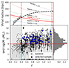 |
Fig. 1. Selection of the isolated galaxy sample. Top: Evolution of the virial radius with redshift for different halo masses compared to the evolution of the size of the MUSE field of view. The solid red line represents the virial radius for the median halo mass of our sample (that we chose as our isolation radius). The vertical dashed lines indicate our redshift selection (0.4 < z < 1.5) for which the isolation radius is contained within the MUSE field of view. Bottom: Distribution of the stellar masses for MEGAFLOW galaxies at z < 1.5. We consider the MEGAFLOW survey reasonably complete for 0.4 < z < 1.5 down to log(M⋆/M⊙) = 9 (represented by the horizontal dashed line). Our volume-limited sample of isolated galaxies is represented by the blue dots. |
Thereafter, we defined our isolated galaxy sample to be the volume-limited sample of isolated galaxies with log(M⋆/M⊙) > 9 at 0.4 < z < 1.5. The selection criteria that we applied successively on the MEGAFLOW catalog to form this sample can be summarized as: 0.4 < z < 1.5 (1124 gals); ZCONF ≥ 2 (960 gals); zgal < zQSO with ΔvQSO ≥ 3000 km s−1 (905 gals); NFOV < 5 to avoid groups; alone within Rvir(Mh, z) (144 galaxies); good UVES coverage (128 galaxies); and log(M⋆/M⊙) > 9 (66 galaxies).
Using these criteria, our sample of isolated galaxies comprised 66 isolated galaxies, with a median mass of log(M⋆/M⊙) = 9.8 and a median redshift of z = 0.91.
4. Galaxy properties
4.1. Stellar masses
For the foreground galaxies having a magnitude r < 26.5 mag, we estimated the stellar masses using the spectral energy distribution (SED) fitting code CONIECTO (for details see Zabl et al. 2016; Bouché et al. 2025). It combines stellar continuum emission from the BC03 model (Bruzual & Charlot 2003) with nebular emission using the method of Schaerer & de Barros (2009), under the assumption of a Chabrier (2003) IMF and a Calzetti et al. (2000) extinction law. The bottom panel of Fig. 1 shows the stellar mass as a function of redshift for the foreground galaxies at z < 1.5 in the MEGAFLOW data. The typical statistical error on log(M⋆/M⊙) is ≈0.15 dex.
4.2. Star formation rate
To estimate the SFR of the galaxies, we used the empirical relation from Gilbank et al. (2010). This relation was derived by calibrating, as a function of mass, the [O II] luminosity against Hα-based SFR corrected from dust extinction using an average Balmer decrement:
![Mathematical equation: $$ \begin{aligned} \mathrm{SFR} = \frac{L([{{\mathrm{O}\,\small{\text{II}}}}]_{\rm obs})/3.8\times 10^{40}\,\mathrm {erg/s}}{a \tanh [(x-b)/c]+d}, \end{aligned} $$](/articles/aa/full_html/2025/02/aa51165-24/aa51165-24-eq5.gif) (1)
(1)
with a = −1.424, b = 9.827, c = 0.572, d = 1.70, and x = log(M⋆/M⊙). The [O II] detection limit imposes an SFR limit of ≈0.01 M⊙/ yr at z = 1. The median SFR of our sample is 3.1 M⊙/ yr.
4.3. GalPaK3D modeling results
In order to derive the galaxies’ morphological and kinematic properties we used the GalPaK3D algorithm (Bouché et al. 2015). GalPaK3D is a Bayesian code that fits a parametric disk model directly to the observed 3D data (x, y, and λ). The disk model assumes an analytic form for the rotation curve, v(r); in our case we used the Universal Rotation Curve (URC) from Salucci & Persic (1997). For that reason, hereafter, we denote the GalPaK3D fits as URC fits. GalPaK3D then convolves the disk model with the instrument point spread function (PSF) and line spread function (LSF) such that it yields the intrinsic parameters of the galaxy. The derived parameters of the disk model are position, inclination, azimuthal angle, effective radius, maximum circular velocity, thermal velocity dispersion, total flux, Sérsic index, [O II] line ratio, turnover radius of the rotation curve, and shape parameter of the rotation curve. The advantage of a 3D fit is that it takes into account all the information present in the data, even if the signal-to-noise ratio (S/N) is low for each individual spaxel.
We first ran GalPaK3D on all 66 of the isolated galaxies in our sample (as defined in Sect. 3). For most of them (63), we used the [O II] doublet, as it is the brightest emission line. We used the [O III] λ5007 and Hβ emission lines, respectively, for two galaxies and one galaxy, for which [O II] is fainter. In this work, we focus on isolated galaxies for which the emission S/N is sufficient to obtain a robust morphology and kinematic model with GalPaK3D. For that reason, we removed galaxies with S/N < 4. After detailed case-by-case visual inspection of the GalPaK3D fits and comparison of modeled velocity maps versus observed velocity maps produced with CAMEL (Epinat et al. 2009, 2012), we removed two additional galaxies that appear to be irregular and hence cannot be modeled by a disk. Lastly, we find that the morphology and kinematics have been convincingly determined for 60 out of our 66 isolated galaxies (Fig. 2).
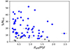 |
Fig. 2. Integrated S/N from pyplatefit versus effective radius divided by PSF full width at half maximum (FWHM) for the 66 isolated galaxies of our isolated galaxy sample. Galaxies for which GalPaK3D fits seem reliable are represented by blue dots. Galaxies with bad fits are represented by gray dots. Galaxies with bad GalPaK3D fits tend to have a low integrated S/N. |
Among the 60 galaxies for which the morphological and kinematic parameters have been determined with GalPaK3D, five galaxies are dispersion dominated, as their circular velocity to velocity dispersion ratio at twice the effective radius, v/σ(2R1/2), is below 1. Lastly, out of the 55 rotation-dominated galaxies, 46 have an inclination angle i > 30, which is sufficient to accurately estimate the azimuthal angle, α, between the major axis and the LOS (see Fig. A.1). We note that the distribution of inclinations for the 60 isolated galaxies modeled with GalPaK3D follows the expected sin i relation (a KS test gives a p-value of 0.25) and that the distribution of azimuthal angles, α, for the 46 galaxies with a sufficient inclination is consistent with a flat distribution (a KS test gives a p-value of 0.56). These distributions are shown in Fig. A.2.
5. Properties of gaseous halos
After selecting the sample of isolated galaxies, we studied their cool gas profile by looking at Mg II absorption in the quasar sight lines. In particular, we quantified the Mg II rest-frame equivalent width and the covering fraction as a function of the impact parameter (see Sects. 5.1 and 5.2, respectively). We then investigated how the Mg II profile depends on redshift and SFR (Sect. 5.3) and on orientation and inclination (Sect. 5.4).
5.1. The rest-frame equivalent width – impact parameter relation ( - b)
- b)
We wanted to establish how Mg II absorption strength varies as a function of the impact parameter. Hereafter, we consider that a galaxy is associated with a Mg II absorption system if the velocity difference between the two is ≤500 km s−1, even though 90% of the velocity differences are ≤200 (100) km s−1 at impact parameters of b < 100 (50) kpc, as discussed in the survey paper (Bouché et al. 2025). As the same paper presents, the 3σ detection limit for Mg II absorption does not evolve significantly between redshift 0.4 and 1.5 with a 75th percentile value of ≈0.075 Å over our 22 fields. We consider this value as an upper limit of detection when no Mg II absorption is detected.
The left panel of Fig. 3 shows  as a function of the impact parameter, b, for our isolated galaxy sample. Below 50 kpc, all log(M⋆/M⊙) > 9 isolated galaxies (21) are associated with Mg II absorption having
  > 0.1 Å. Between 50 and 100 kpc, there is a mix of galaxies with and without absorption above this
  value. Above 100 kpc, the vast majority of galaxies are not associated with absorption above our detection limit and the few cases of detected Mg II absorption have
  < 0.2 Å.
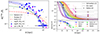 |
Fig. 3. Mg II absorption profile around isolated galaxies. Left: |


To model the relation between absorption equivalent width and impact parameter, we performed a fit similar to that proposed by Chen et al. (2010b) and Dutta et al. (2020), assuming a log-linear relation of the form
 (2)
(2)
where b is the impact parameter. We fitted by maximizing the following likelihood:
![Mathematical equation: $$ \begin{aligned} \begin{split} \mathcal{L} (W)&= \left[ \prod _{i = 1}^n \frac{1}{\sqrt{2 \pi }\sigma _i} \exp \left(-\frac{1}{2} \left[\frac{W_i - W(b_i)}{\sigma _i} \right]^2\right)\right] \\&\quad \times \left[ \prod _{i=1}^m \int _{-\infty }^{W_{i}} \frac{dW\prime }{\sqrt{2 \pi }\sigma _i} \exp \left(-\frac{1}{2} \left[\frac{W\prime - W(b_i)}{\sigma _i} \right]^2\right)\right], \end{split} \end{aligned} $$](/articles/aa/full_html/2025/02/aa51165-24/aa51165-24-eq15.gif) (3)
(3)
where  and σi its associated uncertainty. The first factor in Eq. (3) corresponds to the likelihood of the n points that have detected Mg II absorption and the second factor corresponds to the likelihood of the m points that do not have Mg II absorption detected but only an upper limit on Wi.
The uncertainty σi to Wi is composed of our measurement uncertainty, σmi, and an intrinsic scatter, σc, added in quadrature:
 (4)
(4)
The intrinsic scatter, σc, was added as a free parameter and fitted simultaneously. We performed this fit for our isolated galaxy sample. The result is presented in Table 1 and shown in Fig. 3, along with similar fits from Nielsen et al. (2013a), Dutta et al. (2021) and Huang et al. (2021). Our result is mostly consistent with the fit from Nielsen et al. (2013a) obtained for a sample of 182 isolated galaxies at 0.07 < z < 1.12. They defined an isolated galaxy as a galaxy that has no neighbor within 100 projected kpc and ±500 km s−1, which is compatible with our definition in many cases. They also probed a similar impact parameter range. The result from Dutta et al. (2021) differs significantly from what we obtain. This could be due to the fact that their galaxies are not isolated (when multiple galaxies are present, they consider the one closest to the line of sight), which could explain their higher equivalent width at high b values. Their sample also probes a different impact parameter range, with very few cases at small b (below 50 kpc), which could explain the discrepancy at these distances. They do not apply any selection on stellar mass, so their sample has a lower median mass (log(M⋆/M⊙) = 9.3) than ours (log(M⋆/M⊙) = 9.8). The result from Huang et al. (2021), based on 211 isolated galaxies from SDSS, is broadly consistent with our result even though the fitting function does not have the same form, their redshift range is lower (z < 0.5), and their isolation criterion is different, with no neighbor within 500 projected kpc and ±1000 km s−1.

5.2. Covering fraction
We now turn to computing the Mg II covering fraction, fc. The covering fraction is defined as the probability, P, of detecting a Mg II absorption above a  threshold, at a given projected distance from a galaxy, and within a redshift range, Δv. Given that there are only two possible outcomes (above some threshold there is an absorption (Y = 1) or not (Y = 0)), several methods exist to estimate the covering fraction (e.g., Wilde et al. 2021; Schroetter et al. 2021; Huang et al. 2021). The most popular method relies on counting the outcomes, Y, in bins of b (e.g., Nielsen et al. 2013b). Here, we computed the differential covering fraction following the method described in Schroetter et al. (2021) and Cherrey et al. (2024), which has the advantage that it does not require any binning. Briefly, it consists in a Bayesian logistic regression where the covering fraction follows the logistic form
 (5)
(5)
where P is the probability of detection, Y = 1, and t is a function of the independent variables, Xi, and of the model parameters, θ. We assumed, as a first step, that the covering fraction is governed by the impact parameter, b, to the first order and follows the form
 (6)
(6)
where k0 is the zero point corresponding to the log distance at which P = 0.5, and k1 is the steepness of the transition of P from 0 to 1. We fitted the parameters k0 and k1 using a Monte Carlo Markov chain (MCMC) procedure, along with a Bernouilli likelihood optimized on 9000 steps. We performed the optimization with the Python module pymc3 (Hoffman & Gelman 2014; Salvatier et al. 2016). Hereafter, we denote b50 as the impact parameter corresponding to a 50% probability of having an absorption, i.e. fc = 50%.
We applied this method (Eqs. (5)–(6)) to compute the Mg II covering fraction as a function of impact parameter, fc(b), for our sample and investigated its dependence with respect to the  threshold, Wt, by computing fc for different values of Wt: 0.1 Å, 0.3 Å, 0.5 Å, 0.8 Å, 1.0 Å, and 1.5 Å (see Table 2). In Fig. 3 (upper right panel), we show fc(b) for these different threshold values. We observe a significant shift of k0 with respect to Wt, with almost no slope variation, k1. We also observe, for our sample, a steeper slope than Schroetter et al. (2021) (dotted line) and Dutta et al. (2020) (solid squares), probably due to our stricter preselection of isolated galaxies and our stellar mass selection (see discussion in Sect. 6).
The lower right panels shows that b50 decreases almost linearly with the threshold value, varying from ≈65 kpc at  Å to ≈20 kpc at
  Å. These measurements are consistent with and complementary (in impact parameter coverage) to the results from Dutta et al. (2020). We also show that b50 values computed from TNG50 (DeFelippis et al. 2020) and EAGLE (Ho et al. 2020) simulations are significantly lower than our measurements for similar threshold values. We note that the 0.1 Å covering fraction derived by Schroetter et al. (2021) for primary galaxies in MEGAFLOW is lower than the covering fraction for our sample. This is mainly due to the mass selection that we applied to obtain a volume-limited sample. If we do not apply this criterion, we obtain a similar covering fraction (see Appendix B for details).
One can argue that the preselection of the quasar fields in MEGAFLOW based on the presence of > 3 strong absorption systems ( > 0.5 Å) could introduce a bias in the results, especially in the covering fraction. Cherrey et al. (2024) present a method to estimate the magnitude of this bias that we outline here. The idea is to simulate several quasar fields, randomly populated by galaxies. Each galaxy could be associated or not with an absorption (
 Å) in the quasar spectrum, which in some cases could be strong (
 Å). To realistically mimic the presence of these absorptions, covering fraction curves down to
  Å and to
  Å are needed. Here, we used the covering fraction computed above. The fields with > 3 strong absorption systems were then selected to reproduce the MEGAFLOW selection. Finally, the covering fraction was recomputed on these selected fields and compared with what would be obtained for randomly selected fields, in order to estimate the bias caused by field selection. For 50 fields of 500 × 500 kpc containing ≈50 galaxies each, we obtain 21 pre-selected fields (similar to MEGAFLOW). The b50 at 0.1Å is 66 ± 5 kpc (error is 2σ) for the selected fields versus 63 ± 5 kpc for the random fields. The estimated bias due to field preselection would hence be minor compared to the statistical uncertainties.
5.3. Dependence on redshift, stellar mass, and star formation rate
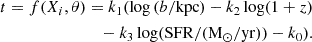
The impact parameter is the most important parameter determining the strength of the absorption and the covering fraction. However, other parameters could also play a role. We investigate the impact of some of them in this section. Figure 4 shows how the absorption strength depends on a number of properties of the galaxies in our sample. It appears in particular that redshift, star formation rate, and stellar mass are correlated with Mg II absorption strength and extent.
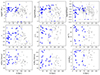 |
Fig. 4. Dependence of Mg II absorption on different galaxy properties. From left to right and top to bottom: log(M*), log(SFR), log(sSFR), redshift z, inclination i, azimuthal angle α, velocity dispersion at 2 Rd, circular velocity at 2 Rd, and v/σ at 2 Rd as a function of the impact parameter for the isolated galaxies. Galaxies associated with absorption with |


In order to investigate these dependencies, we took them into account for the fit of the  -b relation and the fit of the covering fraction. SFR and M⋆ are tightly correlated through the main sequence, so, in order to limit the uncertainties in the fits, we only focused here on the redshift and SFR dependence. In consequence, we replaced Eq. (2) with
 (7)
(7)
And for the covering fraction, we replaced Eq. (6) with
 (8)
(8)
We performed these new fits on our isolated galaxy sample. The fitted parameters for the  -b relation and for the covering fraction are presented in Table 1 and Table 2, respectively, and the resulting fits are shown in Fig. 5. Despite uncertainties compatible with a flat evolution, we observe a tentative decreasing trend of
  and b50 toward low redshifts. Such results give hints that Mg II halos do not follow the growth of dark matter (DM) halos along cosmic time (see discussion below).
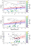 |
Fig. 5. Dependence of Mg II absorption on galaxy redshift, SFR and stellar mass. The top and middle panels present the fitted dependence of Mg II absorption with z and log(SFR), respectively, for our isolated galaxy sample. The bottom panel shows how it converts in terms of M⋆ for the isolated galaxy sample extended to low mass galaxies (without the log(M⋆/M⊙) > 9 selection cut). In the top and middle panels, the solid red lines and the blue dashed lines represent, respectively, the impact parameter at which the |


The bottom panel of Fig. 5 shows how the SFR dependence of  converts into stellar mass dependence. For that, we used the main sequence fitted by Boogaard et al. (2018) and injected it in Eq. (7).
5.4. Dependence on orientation and inclination angles
Several previous observations have suggested that the CGM shows an azimuthal bimodality (e.g., Bouché et al. 2012; Kacprzak et al. 2012; Schroetter et al. 2019). Indeed, galactic winds with higher metallicity are preferentially ejected along the minor axis of galaxies (e.g., Rubin et al. 2014; Schroetter et al. 2016; Guo et al. 2023; Zabl et al. 2021), while accretion rather happens preferentially in corotating disks along the galactic plane (e.g., Ho et al. 2017; Zabl et al. 2019; Nateghi et al. 2024a; Das et al. 2024). For that reason, one might expect Mg II absorption to depend on both inclination, i, and azimuthal angle, α. In Fig. 4 we see that galaxies with low inclination values have weaker absorption than galaxies with high inclination. Indeed, there is only one case of absorption between 50 and 100 kpc for i < 30°. In Fig. 4 we also see that Mg II absorptions are detected out to larger distances for high α than for low α. In order to better visualize the α dependence, Fig. 6 presents the distribution of azimuthal angle for galaxies with and without Mg II absorption systems. We see that the absorption cases are preferentially located along the minor axis, while nonabsorption cases are preferentially observed for intermediate azimuthal angles (30 < α < 60).
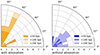 |
Fig. 6. Number of galaxies as a function of the azimuthal angle for the 46 rotation-dominated isolated galaxies with i > 30° and with an associated absorption (left) or without an associated absorption (right). |
To quantify these dependences, we split the rotation-dominated galaxies from our sample (55 in total) into four subsamples: a low-inclination subsample (i < 30°, 9 galaxies) for which the azimuthal angle could not be determined robustly and three subsamples with i > 30°: low α (< 30, 13 galaxies), intermediate α (30 < α < 60°, 13 galaxies), and high α (> 60°, 20 galaxies). The  -b relation for these subsamples is shown in the left panel of Fig. 7. It appears that the high-α sample, for which the line of sight roughly intersects the galaxy’s minor axis, is associated with higher
  values than the low-α sample, for which the line of sight roughly intersects the galaxy’s major axis. The only two cases of absorption at impact parameters above 80 kpc are for high-α galaxies. Low-α galaxies seems to have slightly weaker absorption than high-α galaxies. This is particularly visible in the range 50–100 kpc where there is only one case of absorption for low α versus five for high α. For the intermediate-α sample, it is difficult to draw conclusions as there are very few cases at a small impact parameter. Nonetheless, in the range 50–100 kpc, there is only one case of absorption associated with a galaxy with intermediate α.
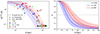 |
Fig. 7. Dependence of the Mg II absorption profile on galaxy inclination and orientation. Left: |

Lastly, we computed the covering fraction using Eq. (6) for the low-α and high-α samples (but not for the intermediate-α and low-inclination samples, as they are not sufficiently populated at low b). The best fitting parameters are presented in Table 2 and the covering fractions are shown in the right panel of Fig. 7. The high-α covering fraction appears to be higher than the low-α covering fraction, suggesting that Mg II is more abundant in outflows than in accretion disks.
6. Discussion
We have shown here that Mg II absorption is ubiquitous for a sample of isolated star-forming galaxies, with log(M⋆/M⊙) > 9 and 0.4 < z < 1.5. Indeed, all galaxies in our sample within an impact parameter of 55 kpc have associated Mg II absorption. Rubin et al. (2014) and Schroetter et al. (2019) suggest that outflowing gas may not be able to escape galactic potential well for sufficiently massive galaxies and would then be re-accreted along the galactic plane in a “fountain” mechanism (Fraternali & Binney 2008) after reaching distances of ≈50 kpc. Our results are consistent with this scenario: first, because Mg II absorption clearly drops between ≈50 and 100 kpc (with only two cases of absorption beyond 100 kpc for our main isolated galaxy sample) and second, because, surprisingly, we find several cases of absorptions at large impact parameters (above 80 kpc and up to 150 kpc) for low-mass isolated galaxies (log(M⋆/M⊙) < 9), even though we observe much fewer absorptions in general for this low-mass sample. This could indicate escaping outflows for these lower potential galaxies. It could also just be a misassignment of the absorption due to the presence of another undetected nearby low-mass galaxy (as MEGAFLOW is not complete below 109 M⊙ in our selected redshift range).
The bottom panel of Fig. 5 shows how the fitted  dependence to SFR converts in M⋆ dependence. In Appendix B, we also show that the covering fraction is significantly higher for log(M⋆/M⊙) > 9 isolated galaxies than for log(M⋆/M⊙) < 9 isolated galaxies. This correlation with stellar mass has already been observed in previous works in absorption (Huang et al. 2021; Lan 2020; Chen et al. 2010c) or in emission using stacking (Guo et al. 2023; Dutta et al. 2023). This is also consistent with the positive correlation between Mg II absorption and luminosity observed, for instance, by Chen et al. (2010b), Nielsen et al. (2013a).
Our results for isolated galaxies complement the results from Dutta et al. (2020, 2021) and Cherrey et al. (2024) for groups. They show that Mg II absorption is more probable and more extended for over-dense regions containing several galaxies and occupying more massive DM halos. This effect could be partly explained by the “superposed” (Bordoloi et al. 2011; Nielsen et al. 2018) contribution of the CGM of the different galaxies and by various interactions producing an “intragroup” medium. Here, we show that even for isolated galaxies more massive halos are more likely to be associated with Mg II absorption at a given impact parameter. The anticorrelation between  and halo mass observed using cross-correlation techniques (Bouché et al. 2006; Lundgren et al. 2009; Gauthier et al. 2009) would then come from the low abundance of massive DM halos compared to light ones.
Recently, Guha et al. (2022) observed that ultrastrong absorbers are associated with massive galaxies with intermediate SFR, but not with starburst galaxies as proposed in other works. Our Fig. 5 reveals that, at small b, galaxies with high SFR (log(SFR/M⊙/yr) > 1) do not show particularly high  . Nevertheless, it appears that Mg II absorption extends further out for high SFR galaxies (up to 100 kpc). This could indicate either that star-formation activity is not so bursty or alternatively that the CGM has a relatively slow response to star-formation activity. Indeed, an outflow ejected at a typical velocity of ≈150 km s−1 takes ≈650 Myr to reach 100 kpc.
Figure 3 (lower right panel) shows the difficulty simulations have in matching the observed Mg II covering fraction. Liang et al. (2016) and DeFelippis et al. (2024) with RAMSES (Teyssier 2002), or DeFelippis et al. (2021) with TNG50 (Marinacci et al. 2018; Naiman et al. 2018) show a cold phase that presents large structures with sharp limits. Contrarily, detailed hydrodynamical models such as McCourt et al. (2018), and analytical models such as Faerman & Werk (2023), tend to favor a “foggy” cold phase with a high number of small clouds (< 1 kpc) that cannot be reproduced by current cosmological simulations. As a consequence, the improvement in resolution seems to enhance the presence of cold gas in the CGM (Hummels et al. 2019; van de Voort et al. 2019). In Fig. 3 (bottom right panel), we show that the GIBLE high-resolution simulations present covering fractions that are closer to our results. These simulations are actually re-simulations of TNG50 galaxies with a 512 better mass resolution. The unresolved nature of the CGM could explain the dominance of the hot phase (T ≈ 105 − 6 K) outside of the central region (≲20 kpc), as presented in the temperature maps from DeFelippis et al. (2024), Ho et al. (2020) and Liang et al. (2016). The implementation of cosmic rays seems to contribute to decreasing the temperature (Farcy et al. 2022; Liang et al. 2016; DeFelippis et al. 2024), and hence to favor the presence of cool clouds.
In Fig. 4 we do not see any clear trend between Mg II absorption and specific SFR (sSFR), indicating that the extent and probability of Mg II absorption is not strongly impacted by the position of the galaxy relative to the main sequence. In particular, we do not observe that passive galaxies (with low sSFR) are associated with weaker Mg II absorption. The positive correlations between  and stellar mass, and between
  and SFR, would then be mainly explained by mass and SFR being correlated along the main sequence.
We also confirm here the previously reported azimuthal bimodality of  and we quantify the Mg II covering fraction along the minor and major axes for galaxies with a sufficient inclination. We find that the covering fraction along the minor axis is significantly higher (at the 2σ level) than the covering fraction along the major axis, which is in agreement with the findings from Kacprzak et al. (2012). With a large sample of star-forming galaxies at z ≈ 1, Lan & Mo (2018) also report that metal absorption is twice as strong along the minor axis within 100 kpc. Huang et al. (2021) report a weak enhancement of Mg II absorption along the minor axis (≲1σ). This weaker trend could be due to the fact that their sample is composed of galaxies with a lower redshift (z < 0.5), so at a later stage of their evolution. Despite a low number of cases, we also find that low-inclination galaxies have lower
  , which is consistent with the conclusions from Nielsen et al. (2015) and with the accretion outflow model of the CGM.
Our results on the redshift evolution (Fig. 5) are consistent with the positive correlation between Mg II absorption and redshift shown in other absorption studies (Nielsen et al. 2013a; Lan 2020; Lundgren et al. 2021; Schroetter et al. 2021; Dutta et al. 2021) and emission studies (Dutta et al. 2023). This result indicates that the CGM (at a given mass) is becoming smaller with cosmic time, which is counterintuitive, as dark matter halos grow with time. It goes against the common assumption that Mg II halos evolve with DM halos (Chen et al. 2010b; Churchill et al. 2013; Faerman & Werk 2023; Huang et al. 2021) and extend to a fixed fraction of the DM halo radius. A possible explanation could come from the relation between SFR and redshift. Indeed, if the extent of Mg II halos is driven by the star-formation activity, it is expected that they are larger at higher redshift when star formation is more important overall. This explanation holds under the assumption that the CGM responds quite quickly to the triggering or stopping of the star-formation activity. Another possible explanation could be that the expansion of the universe causes a decrease in CGM density, preventing Mg II absorption at large b due to ionization. For instance, Stern et al. (2021) explain that if we assume an isothermal density profile 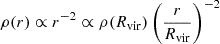 , then the cosmological evolution of ρ(Rvir) implies that ρ(r)∝(1 + z)3 (r/Rvir)−2. Given that the gas become self-shielded (Schaye 2001) against ionizing radiation at a certain density, nsh, then the radius at which ρ(r) reaches nsh evolves like rsh ∝ (1 + z)3/2Rvir. As
 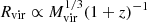 , the evolution of this self-shielding radius is
  , similar to the evolution of the covering fraction b50 ∝ (1 + z)0.8 ± 0.7 that we find for our sample.
Figure 3 (upper right panel) shows that the slope of the transition from 1 to 0 of the covering fraction is steeper for our sample than reported in previous works, such as Schroetter et al. (2021) or Dutta et al. (2020). The steepness of the covering fraction slope indicates how “homologous” CGMs are with each other. Indeed, a shallow covering fraction means that there are both absorptions and nonabsorption cases at all b, while a step function would mean that the presence of absorption is completely determined by the impact parameter. In our case, the steep slope could be interpreted as the fact that our strictly selected sample of isolated galaxies with log(M⋆/M⊙) > 9 have homologous CGMs. In other words, selecting a population of isolated galaxies also selects self-similar CGMs.
Finally, we do not find any clear trend between the Mg II absorption strength and v(2Rd), σ(2Rd), or v/σ(2Rd). We could have expected some correlation with these kinematic parameters. Indeed, as Mg II absorption is often saturated, the  could have been impacted by the velocity dispersion of Mg II clouds along the LOS.
The different observations above lead us to a picture of a cool CGM that is anisotropic, mainly driven by star-formation activity (that is not so bursty, consistent with the relatively moderate dispersion around the MS), and with a short reconfiguration time.
Within the potential bias and limitations of this work, one can first mention the arbitrary maximum LOS velocity window of 500 km/s chosen to associate galaxies with absorption. Recent simulation studies (Ho et al. 2020; Weng et al. 2024) indicate that absorption in this velocity window could be caused by gas outside the virial radius and/or associated with satellites. The fact that we impose no neighbor within ±500 km/s mitigates this risk of misassignment. We also underline that this bias is mostly present for low-mass central galaxies. Ho et al. (2020) estimate that, for galaxies in the mass range  (corresponding to our median mass of
  ), only ≈15% of absorption could be caused by gas outside of Rvir. In our sample, we do not find any cases of galaxies located at high b and associated with strong absorption that could indicate such misassignment.
Regarding completeness, we can distinguish two different effects that could lead to some bias in our sample. First, the double galaxy detection procedure (from continuum and from [O II] emission lines) used in MEGAFLOW, could miss more low SFR galaxies at high z than at low z. This is only true for low-mass galaxies and hence does not impact the correlation with SFR shown in Sect. 5.3. Second, the isolation criterion is a bit looser at high z, as the completeness of low-mass neighbors is lower at these redshifts.
The criterion NFOV < 5 (used to remove galaxies located near groups) depends on the FOV and, hence, evolves with redshift. However this criterion has a small effect overall, as removing it from the analysis only adds 4 new galaxies to the 66 of our sample.
As explained in Sect. 3, the isolation distance is used to define a cylinder around the LOS in which the galaxy is alone. Another neighbor galaxy could hence be present in the virial radius of the selected one and could contribute to the absorption. However, this contribution is believed to be small, as the neighbor would be far from the LOS. Finally, the choice of a redshift-dependent isolation distance is based on the idea that gas halos approximately follow the growth of DM halos. Our results suggest that this is probably not the case, especially at low redshifts where gas halos seem to follow the decrease of SFR. Our isolation distance may then be too conservative and could be relaxed to increase the statistic. As a test, we performed the same analysis with a fixed isolation distance of 125 kpc and do not observe any qualitative change in the results.
Altogether, the potential biases from preselection, completeness, and isolation criterion are small and they have at most a minor influence on the results of this analysis.
7. Conclusions
We have presented here our results for Mg II absorption near isolated galaxies in the MEGAFLOW sample. MEGAFLOW is a quasar absorption survey focused on the Mg II doublet to study the cool CGM. In the 22 quasar fields observed with both MUSE and UVES, a total of 127 Mg II absorption systems and 1208 foreground galaxies have been identified (both from their continuum and emission lines). We focus here on a subsample of 66 isolated galaxies at 0.4 < z < 1.5 with log(M⋆/M⊙) > 9. We used the GalPaK3D algorithm to derive the morphological and kinematic parameters for each galaxy. We then studied how Mg II absorption is impacted by these parameters. Our analysis on this sample leads to the following conclusions:
-
All isolated galaxies with log(M⋆/M⊙) > 9 having an impact parameter below 55 kpc are associated with a Mg II absorption with
 > 0.1 Å (Fig. 3a).
 -
We fitted the
 -b relation and obtained results consistent with similar works on isolated galaxies such as Nielsen et al. (2013a) and Huang et al. (2021), despite different isolation criteria (Fig. 3a).
 -
The Mg II covering fraction (i.e., the probability of obtaining absorption at a given impact parameter) is highly dependent on the absorption strength limit (Fig. 3b). The 50% probability is reached at ≈30 kpc for 1 Å versus ≈65 kpc for 0.1 Å.
-
Isolated galaxies with a large azimuthal angle (α > 60°) relative to the LOS present more extended Mg II absorption than galaxies with mid (30 < α < 60°) or small azimuthal angles (α < 30°) (Figs. 6, 7).
-
The extent, strength, and probability of absorption are correlated with the SFR, consistent with the picture of galactic winds ejecting metals into the CGM to large distances (Fig. 5).
-
The Mg II halos seem to contract from high redshifts to low redshifts (Fig. 5a) (as found in Schroetter et al. 2021; Lundgren et al. 2021) and in consequence do not grow in step with DM halos. This might be due to the overall decrease of star-formation activity toward the local universe and/or to density evolution of the CGM with cosmic time.
-
We do not observe any correlation between Mg II absorption strength and galaxy circular velocity, velocity dispersion, or v/σ (Fig. 4).
Even though galaxies are often found in small groups of few members, we decided here to select isolated galaxies in order to get a sample that could be compared with idealized galaxy simulations. We hope that our results will be used in that context to better understand the underlying physics of the CGM.
Data availability
The 66 isolated galaxies used here can be visualized at https://zenodo.org. The underlying data used for this article are available in the ESO archive (http://archive.eso.org). The MEGAFLOW catalogs and reduced cubes are available at https://megaflow.univ-lyon1.fr/. The catalog can be queried interactively at https://amused.univ-lyon1.fr/project/megaflow/. The data generated for this work will be shared on reasonable request to the corresponding author.
Acknowledgments
This work has been carried out thanks to the support of the ANR 3DGasFlows (ANR-17-CE31-0017). The calculations and figures have been made using the open-source softwares NUMPY (van der Walt et al. 2011; Harris et al. 2020), SCIPY (Virtanen et al. 2020), MATPLOTLIB (Hunter 2007), ASTROPY (Astropy Collaboration 2013, 2018) and PYMC3 (Hoffman & Gelman 2014; Salvatier et al. 2016). The data used in this work are based on observations made with ESO telescopes at the La Silla Paranal Observatory. LW and IP acknowledge funding by the European Research Council through ERC-AdG SPECMAP-CGM, GA 101020943.
References
- Afruni, A., Lopez, S., Anshul, P., et al. 2023, A&A, 680, A112 [NASA ADS] [CrossRef] [EDP Sciences] [Google Scholar]
- Astropy Collaboration (Robitaille, T. P., et al.) 2013, A&A, 558, A33 [NASA ADS] [CrossRef] [EDP Sciences] [Google Scholar]
- Astropy Collaboration (Price-Whelan, A. M., et al.) 2018, AJ, 156, 123 [Google Scholar]
- Bacon, R., Accardo, M., Adjali, L., et al. 2010, in Ground-based and Airborne Instrumentation for Astronomy III, eds. I. S. McLean, S. K. Ramsay, & H. Takami, SPIE Conference Series, 7735, 773508 [Google Scholar]
- Beckett, A., Morris, S. L., Fumagalli, M., et al. 2021, MNRAS, 506, 2574 [NASA ADS] [CrossRef] [Google Scholar]
- Behroozi, P., Wechsler, R. H., Hearin, A. P., & Conroy, C. 2019, MNRAS, 488, 3143 [NASA ADS] [CrossRef] [Google Scholar]
- Bergeron, J., & Boissé, P. 1991, A&A, 243, 344 [NASA ADS] [Google Scholar]
- Bergeron, J., & Stasińska, G. 1986, A&A, 169, 1 [NASA ADS] [Google Scholar]
- Boogaard, L. A., Brinchmann, J., Bouché, N., et al. 2018, A&A, 619, A27 [NASA ADS] [CrossRef] [EDP Sciences] [Google Scholar]
- Bordoloi, R., Lilly, S. J., Knobel, C., et al. 2011, ApJ, 743, 10 [CrossRef] [Google Scholar]
- Bouché, N., Murphy, M. T., Péroux, C., Csabai, I., & Wild, V. 2006, MNRAS, 371, 495 [CrossRef] [Google Scholar]
- Bouché, N., Hohensee, W., Vargas, R., et al. 2012, MNRAS, 426, 801 [CrossRef] [Google Scholar]
- Bouché, N., Carfantan, H., Schroetter, I., Michel-Dansac, L., & Contini, T. 2015, AJ, 150, 92 [Google Scholar]
- Bouché, N. F., Wendt, M., Zabl, J., et al. 2025, A&A, 694, A67 [NASA ADS] [CrossRef] [EDP Sciences] [Google Scholar]
- Bruzual, G., & Charlot, S. 2003, MNRAS, 344, 1000 [NASA ADS] [CrossRef] [Google Scholar]
- Calzetti, D., Armus, L., Bohlin, R. C., et al. 2000, ApJ, 533, 682 [NASA ADS] [CrossRef] [Google Scholar]
- Chabrier, G. 2003, PASP, 115, 763 [Google Scholar]
- Chen, Y.-M., Tremonti, C. A., Heckman, T. M., et al. 2010a, AJ, 140, 445 [Google Scholar]
- Chen, H.-W., Helsby, J. E., Gauthier, J.-R., et al. 2010b, ApJ, 714, 1521 [NASA ADS] [CrossRef] [Google Scholar]
- Chen, H.-W., Wild, V., Tinker, J. L., et al. 2010c, ApJ, 724, L176 [NASA ADS] [CrossRef] [Google Scholar]
- Cherrey, M., Bouché, N. F., Zabl, J., et al. 2024, MNRAS, 528, 481 [NASA ADS] [CrossRef] [Google Scholar]
- Churchill, C. W., Trujillo-Gomez, S., Nielsen, N. M., & Kacprzak, G. G. 2013, ApJ, 779, 87 [NASA ADS] [CrossRef] [Google Scholar]
- Das, S., Rickel, M., Leroy, A., et al. 2024, MNRAS, 527, 10358 [Google Scholar]
- DeFelippis, D., Genel, S., Bryan, G. L., et al. 2020, ApJ, 895, 17 [NASA ADS] [CrossRef] [Google Scholar]
- DeFelippis, D., Bouché, N. F., Genel, S., et al. 2021, ApJ, 923, 56 [NASA ADS] [CrossRef] [Google Scholar]
- DeFelippis, D., Bournaud, F., Bouché, N., et al. 2024, MNRAS, 530, 52 [NASA ADS] [CrossRef] [Google Scholar]
- Dekker, H., D’Odorico, S., Kaufer, A., Delabre, B., & Kotzlowski, H. 2000, in Optical and IR Telescope Instrumentation and Detectors, eds. M. Iye, & A. F. M. Moorwood, International Society for Optics and Photonics (SPIE), 4008, 534 [NASA ADS] [CrossRef] [Google Scholar]
- Dutta, R., Fumagalli, M., Fossati, M., et al. 2020, MNRAS, 499, 5022 [CrossRef] [Google Scholar]
- Dutta, R., Fumagalli, M., Fossati, M., et al. 2021, MNRAS, 508, 4573 [NASA ADS] [CrossRef] [Google Scholar]
- Dutta, R., Fossati, M., Fumagalli, M., et al. 2023, MNRAS, 522, 535 [NASA ADS] [CrossRef] [Google Scholar]
- Epinat, B., Contini, T., Le Fèvre, O., et al. 2009, A&A, 504, 789 [NASA ADS] [CrossRef] [EDP Sciences] [Google Scholar]
- Epinat, B., Tasca, L., Amram, P., et al. 2012, A&A, 539, A92 [NASA ADS] [CrossRef] [EDP Sciences] [Google Scholar]
- Faerman, Y., & Werk, J. K. 2023, ApJ, 956, 92 [NASA ADS] [CrossRef] [Google Scholar]
- Farcy, M., Rosdahl, J., Dubois, Y., Blaizot, J., & Martin-Alvarez, S. 2022, MNRAS, 513, 5000 [NASA ADS] [CrossRef] [Google Scholar]
- Faucher-Giguère, C.-A., & Oh, S. P. 2023, ARA&A, 61, 131 [CrossRef] [Google Scholar]
- Fraternali, F., & Binney, J. J. 2008, MNRAS, 386, 935 [CrossRef] [Google Scholar]
- Gauthier, J.-R., Chen, H.-W., & Tinker, J. L. 2009, ApJ, 702, 50 [NASA ADS] [CrossRef] [Google Scholar]
- Gilbank, D. G., Baldry, I. K., Balogh, M. L., Glazebrook, K., & Bower, R. G. 2010, MNRAS, 405, 2594 [NASA ADS] [Google Scholar]
- Guha, L. K., Srianand, R., Dutta, R., et al. 2022, MNRAS, 513, 3836 [NASA ADS] [CrossRef] [Google Scholar]
- Guo, Y., Bacon, R., Bouché, N. F., et al. 2023, Nature, 624, 53 [NASA ADS] [CrossRef] [Google Scholar]
- Harris, C. R., Millman, K. J., van der Walt, S. J., et al. 2020, Nature, 585, 357 [NASA ADS] [CrossRef] [Google Scholar]
- Hinshaw, G., Larson, D., Komatsu, E., et al. 2013, ApJS, 208, 19 [Google Scholar]
- Ho, S. H., Martin, C. L., Kacprzak, G. G., & Churchill, C. W. 2017, ApJ, 835, 267 [NASA ADS] [CrossRef] [Google Scholar]
- Ho, S. H., Martin, C. L., & Turner, M. L. 2019, ApJ, 875, 54 [NASA ADS] [CrossRef] [Google Scholar]
- Ho, S. H., Martin, C. L., & Schaye, J. 2020, ApJ, 904, 76 [NASA ADS] [CrossRef] [Google Scholar]
- Hoffman, M. D., & Gelman, A. 2014, JMLR, 15, 1593 [Google Scholar]
- Huang, Y.-H., Chen, H.-W., Shectman, S. A., et al. 2021, MNRAS, 502, 4743 [NASA ADS] [CrossRef] [Google Scholar]
- Hummels, C. B., Smith, B. D., Hopkins, P. F., et al. 2019, ApJ, 882, 156 [NASA ADS] [CrossRef] [Google Scholar]
- Hummels, C. B., Rubin, K. H. R., Schneider, E. E., & Fielding, D. B. 2024, ApJ, 972, 148 [NASA ADS] [CrossRef] [Google Scholar]
- Hunter, J. D. 2007, CiSE, 9, 90 [Google Scholar]
- Kacprzak, G. G., Churchill, C. W., & Nielsen, N. M. 2012, ApJ, 760, L7 [NASA ADS] [CrossRef] [Google Scholar]
- Kacprzak, G. G., Cooke, J., Churchill, C. W., Ryan-Weber, E. V., & Nielsen, N. M. 2013, ApJ, 777, L11 [Google Scholar]
- Lan, T.-W. 2020, ApJ, 897, 97 [NASA ADS] [CrossRef] [Google Scholar]
- Lan, T.-W., & Fukugita, M. 2017, ApJ, 850, 156 [NASA ADS] [CrossRef] [Google Scholar]
- Lan, T.-W., & Mo, H. 2018, ApJ, 866, 36 [NASA ADS] [CrossRef] [Google Scholar]
- Liang, C. J., Kravtsov, A. V., & Agertz, O. 2016, MNRAS, 458, 1164 [CrossRef] [Google Scholar]
- Lundgren, B. F., Brunner, R. J., York, D. G., et al. 2009, ApJ, 698, 819 [NASA ADS] [CrossRef] [Google Scholar]
- Lundgren, B. F., Creech, S., Brammer, G., et al. 2021, ApJ, 913, 50 [NASA ADS] [CrossRef] [Google Scholar]
- Marinacci, F., Vogelsberger, M., Pakmor, R., et al. 2018, MNRAS, 480, 5113 [NASA ADS] [Google Scholar]
- McCourt, M., Oh, S. P., O’Leary, R., & Madigan, A.-M. 2018, MNRAS, 473, 5407 [Google Scholar]
- Ménard, B., & Chelouche, D. 2009, MNRAS, 393, 808 [CrossRef] [Google Scholar]
- Naiman, J. P., Pillepich, A., Springel, V., et al. 2018, MNRAS, 477, 1206 [Google Scholar]
- Nateghi, H., Kacprzak, G. G., Nielsen, N. M., et al. 2024a, MNRAS, 533, 1321 [NASA ADS] [CrossRef] [Google Scholar]
- Nateghi, H., Kacprzak, G. G., Nielsen, N. M., et al. 2024b, MNRAS, 534, 930 [NASA ADS] [CrossRef] [Google Scholar]
- Nielsen, N. M., Churchill, C. W., & Kacprzak, G. G. 2013a, ApJ, 776, 115 [NASA ADS] [CrossRef] [Google Scholar]
- Nielsen, N. M., Churchill, C. W., Kacprzak, G. G., & Murphy, M. T. 2013b, ApJ, 776, 114 [NASA ADS] [CrossRef] [Google Scholar]
- Nielsen, N. M., Churchill, C. W., Kacprzak, G. G., Murphy, M. T., & Evans, J. L. 2015, ApJ, 812, 83 [NASA ADS] [CrossRef] [Google Scholar]
- Nielsen, N. M., Kacprzak, G. G., Pointon, S. K., Churchill, C. W., & Murphy, M. T. 2018, ApJ, 869, 153 [NASA ADS] [CrossRef] [Google Scholar]
- Péroux, C., Nelson, D., van de Voort, F., et al. 2020, MNRAS, 499, 2462 [CrossRef] [Google Scholar]
- Ramesh, R., & Nelson, D. 2024, MNRAS, 528, 3320 [NASA ADS] [CrossRef] [Google Scholar]
- Rubin, K. H. R., Prochaska, J. X., Koo, D. C., et al. 2014, ApJ, 794, 156 [Google Scholar]
- Salucci, P., & Persic, M. 1997, in Dark and Visible Matter in Galaxies and Cosmological Implications, eds. M. Persic, & P. Salucci, ASPCS, 117, 1 [NASA ADS] [Google Scholar]
- Salvatier, J., Wiecki, T. V., & Fonnesbeck, C. 2016, PeerJ Comput. Sci., 2, e55 [Google Scholar]
- Schaerer, D., & de Barros, S. 2009, A&A, 502, 423 [NASA ADS] [CrossRef] [EDP Sciences] [Google Scholar]
- Schaye, J. 2001, ApJ, 559, 507 [NASA ADS] [CrossRef] [Google Scholar]
- Schroetter, I., Bouché, N., Wendt, M., et al. 2016, ApJ, 833, 39 [NASA ADS] [CrossRef] [Google Scholar]
- Schroetter, I., Bouché, N. F., Zabl, J., et al. 2019, MNRAS, 490, 4368 [CrossRef] [Google Scholar]
- Schroetter, I., Bouché, N. F., Zabl, J., et al. 2021, MNRAS, 506, 1355 [NASA ADS] [CrossRef] [Google Scholar]
- Steidel, C. C. 1995, in QSO Absorption Lines, ed. G. Meylan, 139 [CrossRef] [Google Scholar]
- Stern, J., Sternberg, A., Faucher-Giguère, C.-A., et al. 2021, MNRAS, 507, 2869 [NASA ADS] [CrossRef] [Google Scholar]
- Teyssier, R. 2002, A&A, 385, 337 [CrossRef] [EDP Sciences] [Google Scholar]
- van der Walt, S., Colbert, S. C., & Varoquaux, G. 2011, CiSE, 13, 22 [Google Scholar]
- van de Voort, F., Springel, V., Mandelker, N., van den Bosch, F. C., & Pakmor, R. 2019, MNRAS, 482, L85 [NASA ADS] [CrossRef] [Google Scholar]
- Virtanen, P., Gommers, R., Oliphant, T. E., et al. 2020, Nat. Meth., 17, 261 [Google Scholar]
- Weng, S., Péroux, C., Ramesh, R., et al. 2024, MNRAS, 527, 3494 [Google Scholar]
- Wilde, M. C., Werk, J. K., Burchett, J. N., et al. 2021, ApJ, 912, 9 [NASA ADS] [CrossRef] [Google Scholar]
- Wisotzki, L., Bacon, R., Brinchmann, J., et al. 2018, Nature, 562, 229 [Google Scholar]
- Zabl, J., Freudling, W., Møller, P., et al. 2016, A&A, 590, A66 [NASA ADS] [CrossRef] [EDP Sciences] [Google Scholar]
- Zabl, J., Bouché, N. F., Schroetter, I., et al. 2019, MNRAS, 485, 1961 [NASA ADS] [CrossRef] [Google Scholar]
- Zabl, J., Bouché, N. F., Wisotzki, L., et al. 2021, MNRAS, 507, 4294 [NASA ADS] [CrossRef] [Google Scholar]
- Zhang, H., Zaritsky, D., Zhu, G., Ménard, B., & Hogg, D. W. 2016, ApJ, 833, 276 [NASA ADS] [CrossRef] [Google Scholar]
- Zhu, G., & Ménard, B. 2013, ApJ, 770, 130 [NASA ADS] [CrossRef] [Google Scholar]
Appendix A: Inclination and azimuthal distribution from GalPaK3D
We present in Fig. A.1 the inclination and azimuthal angle α between the major axis and the position of the quasar sight-line. Figure A.2 presents the inclination i and azimuthal angle α distribution for our sample.
 |
Fig. A.1. Schematic representation of the azimuthal angle α relative to the position of the QSO and inclination angle i viewed in the plane of the sky (along the line-of-sight) on the left (right), respectively. |
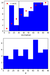 |
Fig. A.2. Top: Distribution of the GalPaK3D estimated inclination for the 60 galaxies modeled with GalPaK3D. Red dots are proportional to the expected sinus distribution. Bottom: Distribution of the azimuth angle α between galaxies major axis and LOS for the 46 isolated rotation dominated galaxies with sufficient inclination angle i > 30. |
Appendix B: Mass dependence of covering fraction
In Fig. 5 we show that the Mg II profile and covering fraction is correlated with the SFR. The SFR is correlated with the stellar mass through the main sequence relation. In order to visualize the mass dependence of Mg II absorption, we compare in Fig. B.1 the covering fraction for our isolated galaxy sample (with log(M⋆/M⊙) > 9) with similarly selected isolated galaxies of low mass (with log(M⋆/M⊙) < 9). We also show the covering fraction computed for the whole isolated galaxy sample (without mass selection) and compare it with the covering fraction computed from Schroetter et al. (2021) (without mass selection neither).
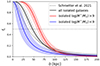 |
Fig. B.1. Covering fraction computed for isolated galaxies with log(M⋆/M⊙) > 9 (our main sample, represented by the red curve), with log(M⋆/M⊙) < 9 (represented by the blue curve) and without mass selection (represented by the black curve). The covering fraction computed by Schroetter et al. (2021) for MEGAFLOW primary galaxies without mass selection is represented by the black dotted line. |
Appendix C: Isolated galaxy catalog
Table C.1 presents the main properties of the isolated galaxy sample. A visual catalog of the sample is also available online (see the data availability section above).
Isolated galaxy sample.
All Tables
All Figures
|
Fig. 1. Selection of the isolated galaxy sample. Top: Evolution of the virial radius with redshift for different halo masses compared to the evolution of the size of the MUSE field of view. The solid red line represents the virial radius for the median halo mass of our sample (that we chose as our isolation radius). The vertical dashed lines indicate our redshift selection (0.4 < z < 1.5) for which the isolation radius is contained within the MUSE field of view. Bottom: Distribution of the stellar masses for MEGAFLOW galaxies at z < 1.5. We consider the MEGAFLOW survey reasonably complete for 0.4 < z < 1.5 down to log(M⋆/M⊙) = 9 (represented by the horizontal dashed line). Our volume-limited sample of isolated galaxies is represented by the blue dots. |
| In the text | |
|
Fig. 2. Integrated S/N from pyplatefit versus effective radius divided by PSF full width at half maximum (FWHM) for the 66 isolated galaxies of our isolated galaxy sample. Galaxies for which GalPaK3D fits seem reliable are represented by blue dots. Galaxies with bad fits are represented by gray dots. Galaxies with bad GalPaK3D fits tend to have a low integrated S/N. |
| In the text | |
|
Fig. 3. Mg II absorption profile around isolated galaxies. Left: |
| In the text | |
|
Fig. 4. Dependence of Mg II absorption on different galaxy properties. From left to right and top to bottom: log(M*), log(SFR), log(sSFR), redshift z, inclination i, azimuthal angle α, velocity dispersion at 2 Rd, circular velocity at 2 Rd, and v/σ at 2 Rd as a function of the impact parameter for the isolated galaxies. Galaxies associated with absorption with |
| In the text | |
|
Fig. 5. Dependence of Mg II absorption on galaxy redshift, SFR and stellar mass. The top and middle panels present the fitted dependence of Mg II absorption with z and log(SFR), respectively, for our isolated galaxy sample. The bottom panel shows how it converts in terms of M⋆ for the isolated galaxy sample extended to low mass galaxies (without the log(M⋆/M⊙) > 9 selection cut). In the top and middle panels, the solid red lines and the blue dashed lines represent, respectively, the impact parameter at which the |
| In the text | |
|
Fig. 6. Number of galaxies as a function of the azimuthal angle for the 46 rotation-dominated isolated galaxies with i > 30° and with an associated absorption (left) or without an associated absorption (right). |
| In the text | |
|
Fig. 7. Dependence of the Mg II absorption profile on galaxy inclination and orientation. Left: |
| In the text | |
|
Fig. A.1. Schematic representation of the azimuthal angle α relative to the position of the QSO and inclination angle i viewed in the plane of the sky (along the line-of-sight) on the left (right), respectively. |
| In the text | |
|
Fig. A.2. Top: Distribution of the GalPaK3D estimated inclination for the 60 galaxies modeled with GalPaK3D. Red dots are proportional to the expected sinus distribution. Bottom: Distribution of the azimuth angle α between galaxies major axis and LOS for the 46 isolated rotation dominated galaxies with sufficient inclination angle i > 30. |
| In the text | |
|
Fig. B.1. Covering fraction computed for isolated galaxies with log(M⋆/M⊙) > 9 (our main sample, represented by the red curve), with log(M⋆/M⊙) < 9 (represented by the blue curve) and without mass selection (represented by the black curve). The covering fraction computed by Schroetter et al. (2021) for MEGAFLOW primary galaxies without mass selection is represented by the black dotted line. |
| In the text | |
Current usage metrics show cumulative count of Article Views (full-text article views including HTML views, PDF and ePub downloads, according to the available data) and Abstracts Views on Vision4Press platform.
Data correspond to usage on the plateform after 2015. The current usage metrics is available 48-96 hours after online publication and is updated daily on week days.
Initial download of the metrics may take a while.