| Issue |
A&A
Volume 663, July 2022
|
|
|---|---|---|
| Article Number | A11 | |
| Number of page(s) | 20 | |
| Section | Extragalactic astronomy | |
| DOI | https://doi.org/10.1051/0004-6361/202142179 | |
| Published online | 01 July 2022 | |
The MUSE eXtremely deep field: first panoramic view of an Mg II emitting intragroup medium⋆
1
Observatoire de Genève, Universite de Genève, Chemin Pegasi 51, 1290 Versoix, Switzerland
e-mail: This email address is being protected from spambots. You need JavaScript enabled to view it.
2
Aix Marseille Univ., CNRS, CNES, LAM, Marseille, France
3
Department of Physics, ETH Zürich, Wolfgang-Pauli-Strasse 27, 8093 Zürich, Switzerland
4
Univ. Lyon, Univ. Lyon1, ENS de Lyon, CNRS, Centre de Recherche Astrophysique de Lyon UMR5574, 69230 Saint-Genis-Laval, France
5
Institute for Computational Astrophysics and Department of Astronomy & Physics, Saint Mary’s University, 923 Robie Street, Halifax, Nova Scotia B3H 3C3, Canada
6
Leibniz-Institut für Astrophysik Potsdam (AIP), An der Sternwarte 16, 14482 Potsdam, Germany
7
Max Planck Institute for Astronomy, Königstuhl 17, 69117 Heidelberg, Germany
8
Leiden Observatory, Leiden University, PO Box 9513 2300 RA Leiden, The Netherlands
9
Instituto de Astrofísica e Ciências do Espaço, Universidade do Porto, CAUP, Rua das Estrelas, 4150-762 Porto, Portugal
10
Dipartimento di Fisica G. Occhialini, Università degli Studi di Milano Bicocca, Piazza della Scienza 3, 20126 Milano, Italy
11
Institut de Recherche en Astrophysique et Planétologie (IRAP), Université de Toulouse, CNRS, UPS, CNES, 31400 Toulouse, France
12
IUCAA, Post Bag 04, Ganeshkhind, Pune 411007, India
13
Centre for Astrophysics and Supercomputing, Swinburne University of Technology, Hawthorn, VIC 3122, Australia
Received:
8
September
2021
Accepted:
20
April
2022
Abstract
Using the exquisite data from the MUSE eXtremely Deep Field (MXDF), we report the discovery of an Mg II emission nebula with an area above a 2σ significance level of 1000 proper kpc2. This provides the first panoramic view of the spatial distribution of magnesium in the intragroup medium of a low-mass group of five star-forming galaxies at z = 1.31. The galaxy group members are separated by less than 50 physical kpc in projection and ≈120 km s−1 in velocity space. The most massive galaxy has a stellar mass of 109.35 M⊙ and shows an Mg II P-Cygni line profile, indicating the presence of an outflow, which is consistent with the spatially resolved spectral analysis showing ≈+120 km s−1 shift of the Mg II emission lines with respect to the systemic redshift. The other galaxies are less massive and only show Mg II in emission. The detected Mg II nebula has a maximal projected extent of ≈70 kpc, including a low-surface-brightness (≈2 × 10⁻¹⁹ erg s−1 cm−2 arcsec−2) gaseous bridge between two subgroups of galaxies. The presence of absorption features in the spectrum of a background galaxy located at an impact parameter of 19 kpc from the closest galaxy of the group indicates the presence of gas enriched in magnesium even beyond the detected nebula seen in emission, which suggests that we are observing the tip of a larger intragroup medium. The observed Mg II velocity gradient suggests an overall rotation of the structure along the major axis of the most massive galaxy. Our MUSE data also reveal extended Fe II* emission in the vicinity of the most massive galaxy, aligned with its minor axis and pointing towards a neighboring galaxy. Extended [O II] emission is found around the galaxy group members and at the location of the Mg II bridge. Our results suggest that both tidal stripping effects from galaxy interactions and outflows are enriching the intragroup medium of this system.
Key words: galaxies: groups: general / Galaxy: formation / galaxies: evolution / galaxies: interactions / intergalactic medium
Based on observations made with ESO telescope at the La Silla Paranal Observatory under the large program 1101.A-0127.
© F. Leclercq et al. 2022
 Open Access article, published by EDP Sciences, under the terms of the Creative Commons Attribution License (https://creativecommons.org/licenses/by/4.0), which permits unrestricted use, distribution, and reproduction in any medium, provided the original work is properly cited.
This article is published in open access under the Subscribe-to-Open model. This email address is being protected from spambots. You need JavaScript enabled to view it. to support open access publication.
1. Introduction
In the ΛCDM framework, theories and simulations predict that galaxies grow in mass and size by accreting cold gas and by merging with other galaxies. The environment is known to play a crucial role in shaping galaxy growth. Indeed, theoretical work indicates that tidal interactions and merging events can dramatically impact the properties of the galaxies and their circumgalactic medium (CGM, e.g., Hani et al. 2018). Studying galaxy systems is therefore crucial for understanding the effect of environment on galaxy formation and evolution.
A large number of galaxy groups found in spectroscopic redshift surveys have been reported in the literature (e.g., Cucciati et al. 2010; Iovino et al. 2016; Abril-Melgarejo et al. 2021). Galaxy groups are generally referred to as the lower mass end (dark matter halo mass ≲1013 M⊙) of galaxy clusters, although the definition of groups in terms of halo mass is vague. A commonly adopted definition of a galaxy group is an association of three or more galaxies with a physical distance of Δr ≲ 500 kpc and a velocity separation of Δv ≲ 500 km s−1 (e.g., Knobel et al. 2009; Diener et al. 2013).
Gas exchanges between the group members and their CGM as well as galaxy interactions shape the intragroup medium (IGrM). It is, thus, a great laboratory for studying the effects of the local environment and gas flows on galaxy formation and evolution. The IGrM is a multi-phase medium. At very low redshifts, it is mainly detected and studied through the X-ray emission from its hot phase (e.g., Lovisari et al. 2015; Eckert et al. 2017; Oppenheimer et al. 2021, and associated papers for a review). Those studies are however limited to massive galaxy groups (dark matter, hereafter DM, halo mass > 1013 M⊙) due to the low X-ray flux at lower masses (Lovisari et al. 2021). Observations of neutral hydrogen in nearby galaxy groups reveal that the cold phase of the IGrM also shows extended structures (Michel-Dansac et al. 2010; Borthakur et al. 2010; Serra et al. 2013). At higher redshifts, most constraints on the associated IGrM come from absorption line studies in lines of sight probed by bright background objects. Several possibilities are proposed and discussed in the literature to explain the origin of the absorbing gas in systems with three or more galaxies: the gas detected in absorption could be associated with the IGrM of the system (Nielsen et al. 2018), the CGM of the group members (Bordoloi et al. 2011; Fossati et al. 2019), tidal tail remnants (Kacprzak et al. 2010; Dutta et al. 2020), or orbiting gas clouds (Bielby et al. 2017) after galaxy interactions.
The advent of integral field unit (IFU) instruments is revolutionizing the study of the circum- and intragroup media by allowing their direct mapping in emission. The unprecedented sensitivity of VLT/MUSE (Bacon et al. 2010) recently allowed for the detection of ionized and enriched intragroup nebula at z ≲ 0.7. Epinat et al. (2018) reported the detection of a 150 kpc large [O II] nebula at z ≈ 0.7 surrounding a dozen galaxies with stellar masses around 1010 M⊙. Chen et al. (2019) reported a 100 kpc Hα blob around a galaxy group with a dynamical mass of ≈3 × 10¹² M⊙ at z ≈ 0.3. While Epinat et al. (2018) do not exclude a possible contribution from active galactic nucleus (AGN) outflows, both analyses favor a scenario where the observed metal enriched gas has been extracted from galaxies by tidal stripping forces. Moreover, Johnson et al. (2018) discovered six and Helton et al. (2021) three spatially extended nebulae emitting in [O III], [O II] and Hβ in z ≈ 0.5 galaxy groups hosting a quasar. Both studies suggest that nebulae are a signature of galaxy interactions in quasar host groups.
At higher redshift, the IGrM of star-forming galaxies is mainly detected in H I Lyman αλ1215.67 Å (Lyα) and generally referred to as Lyα blobs (LABs, e.g., Steidel et al. 2010; Caminha et al. 2016; Vanzella et al. 2017; Herenz et al. 2020). The Lyα line traces the neutral phase of the IGrM at z > 0.3; at z = 0, Lyα observations are extremely limited. In order to connect the ionized intragroup media observed at lower redshifts to those of high redshift galaxy systems, a tracer of the neutral gas phase observable at low-z is needed. The Mg IIλλ2796, 2803 (hereafter Mg II) doublet is a very good candidate. Indeed, because of the lower ionization potential of Mg I (7.6 eV) compared to H I (13.6 eV), hydrogen gas is neutral when Mg II photons are emitted, namely, Mg II traces the H I gas. Because Mg II is a resonant line, we expect to observe extended Mg II emission, similarly to Lyα (e.g., Wisotzki et al. 2016; Leclercq et al. 2017).
The detection of extended Mg II emission was reported for the first time ten years ago by Rubin et al. (2011) and later by Martin et al. (2013), both using slit spectroscopy of galaxies at z ≈ 0.7 and 0.9, respectively. Statistical evidence for such Mg II halos at slightly higher redshift (z ≈ 1.5) was demonstrated by Erb et al. (2012) via the stacking of long-slit spectra. Their analyses were, however, limited by the slit aperture, preventing us from getting a complete view of the galaxy surroundings. By reporting non-detections in narrow band (NB) images of five star-forming galaxies at z ≈ 0.7, Rickards Vaught et al. (2019) reinforced the assumption that the detection of the extended Mg II gas is challenging. Recently, Burchett et al. (2021) re-observed the Rubin et al. (2011)z = 0.7 galaxy using the Keck Cosmic Webb Imager (Keck/KCWI, Martin et al. 2010) and confirmed the detection of significant extended Mg II emission spanning over ≈40 kpc. They were able to perform the first detailed spatially resolved analysis of an Mg II halo and found that isotropic outflow models best fit the data. This detection has been followed up by two similar discoveries (Zabl et al. 2021; Wisotzki et al., in prep.) in the MUSE GAs FLOw and Wind (MEGAFLOW) survey and MUSE-Deep fields (Bacon et al. 2017), respectively. Zabl et al. (2021) reported the first discovery of an Mg II emission halo probed by a quasar sightline around a z = 0.702 galaxy. Thanks to the 3D MUSE view on the CGM of this galaxy, the authors were able to compare the observations with toy models and found good consistency with a bi-conical outflow model. These very recent discoveries highlight the fact that IFU instruments truly are game changers for the study of the circum- and intragroup medium of galaxies.
In this paper, we report the discovery of the first intragroup medium mapped in Mg II, detected in the MUSE eXtremely Deep Field (MXDF, Bacon et al., in prep. and see also Bacon et al. 2021). The emitting nebula encompasses a group of five low-mass galaxies (M* < 109.4 M⊙) at z ≈ 1.31 with a halo mass of ≈1011.7 M⊙. It extends over ≈70 kpc (physical) and unveils gaseous connections between galaxies. By taking advantage of the three-dimensional (3D) information provided by the MUSE data cubes, we study the kinematics of the nebula. Diffuse [O II] λλ3726, 3729 (hereafter [O II]) and Fe II* (λ2365, λ2396, λ2612, λ2626, hereafter Fe II*) emission are also detected and allow a comparison between the different gas phases of the IGrM. This first detection of an Mg II emitting intragroup nebula – until now, only locally probed along absorption lines of sight – allows us to shed light on the highly debated existence of an IGrM in low-mass galaxy groups and on its origin.
The paper is organized as follows. We describe the MXDF observations, data reduction, and catalog classification in Sect. 2. The group and the properties of the galaxy members studied in this paper are presented in Sect. 3. Section 4 describes the detection and analysis of the Mg II intragroup nebula. In Sect. 5, we investigate the [O II] and Fe II* properties of the group and compare them with Mg II. Then, in Sect. 6, we discuss the existence and origin of the intragroup medium and the mechanisms that make it shine. Section 6 also provides a comparison with the literature. Finally, we present our summary and conclusions in Sect. 7.
Throughout the paper, all magnitudes are expressed in the AB system and distances are in physical units that are not comoving. We assume a flat ΛCDM cosmology with Ωm = 0.315 and H0 = 67.4 km s−1 Mpc−1 (Planck Collaboration VI 2020); in this framework, a 1″ angular separation corresponds to 8.6 kpc proper at the redshift of the group (z ≈ 1.31).
2. MXDF observations
Here, we provide a summary of the data acquisition, data reduction, and catalog building processes. More details can be found in Bacon et al. (2021) and in the upcoming survey paper Bacon et al. (in prep.).
The MXDF data were taken as part of the MUSE Guaranteed Time Observations program between August 2018 and January 2019 under photometric conditions. The observations were performed with the VLT GALACSI/AOF ground-layer adaptive optics system (Kolb et al. 2016; Madec et al. 2018). A single 140-h pointing was completed after rejection of bad quality exposures. The MUSE field of view was rotated between each observation in order to reduce the systematics. The resulting quasi-circular field is more than 100 h deep in the inner 31″ radius and the exposure time decreases to ≈10 h at a radius of 41″. The MXDF data partially overlaps with the MUSE 10-h and 30-h fields from Bacon et al. (2017), denoted mosaic and udf-10, respectively, as well as with the 1-h MUSE-Wide fields (Urrutia et al. 2019, and in prep.).
The data reduction is similar to the one described in Bacon et al. (2017); it is based on the MUSE public pipeline (Weilbacher et al. 2020) and includes some improvements resulting in reduced systematics and a better sky subtraction. We estimated the point spread function (PSF) using the muse-psfrec software (Fusco et al. 2020). The final PSF is modeled using a Moffat function (Moffat 1969) with parameters of  (
( ) full width at half maximum (FWHM) and β = 2.1 (1.8) at the blue (red) end of the datacube. The datacube contains 157034 spatial pixels (spaxel) of
  . The number of spectra matches the number of spaxels with a wavelength range of 4700 Å to 9350 Å divided into 3721 pixels of 1.25 Å. The datacube also contains the estimated variance for each pixel.
The MXDF source catalog (Bacon et al., in prep.) consists of (i) sources blindly detected and extracted using the ORIGIN software (Mary et al. 2020) which is designed to detect emission lines in 3D data sets and (ii) sources extracted using the ODHIN software (Bacher 2017) based on an HST catalog (Rafelski et al. 2015), which performs source deblending in MUSE using high resolution HST images. The ODHIN approach is similar to TDOSE (Schmidt et al. 2019) developed for the MUSE wide survey (Urrutia et al. 2019; Schmidt et al. 2021) with the differences that it is non-parametric, it uses multiple broadband HST images, and it implements a regularization process to avoid noise amplification for very close sources. The sources are then inspected by three experts and a final catalog of 733 sources with redshift and associated confidence is created. It includes 406 new spectroscopic redshift measurements with respect to the previous MUSE deep field catalog (Inami et al. 2017).
3. A group of galaxies at z ≈ 1.3
The Mg II nebula was discovered during the search for extended Mg II emission around galaxies in the MUSE Hubble Ultra Deep Field (UDF, Bacon et al. 2017). A visual inspection, first in the udf-10 and then in the newly observed MXDF data (see Appendix A), revealed, at first glance, Mg II emission offset from a galaxy and extended in one direction. By increasing the size of the search area and looking for neighbors, we found this object to be surrounded by four close galaxies. In this section, we focus on the environment (Sect. 3.1), global properties and integrated spectral features of the group members (Sects. 3.2 and 3.3, respectively). The Mg II intragroup nebula detected in the five-member galaxy group is presented and analyzed in the next section (Sect. 4).
3.1. The galaxy group and its environment
The group we are studying here consists of five galaxies at redshift z ≈ 1.31. Using a friends-of-friends algorithm (Huchra & Geller 1982) connecting galaxies separated by less than 450 kpc and 500 km s−1 in the MXDF, UDF, and MUSE-Wide catalogs (Bacon et al., in prep.; Urrutia et al. 2019, and in prep.), we found that this group is at the center of a larger structure of 14 galaxies with spectroscopically confirmed redshifts (with high confidence, ZCONF > 1 in the MUSE catalogs, except for one object, see below) and separated by less than 460 km s−1 in redshift space. This structure spans the MUSE UDF mosaic field over 1.9 Mpc in projection (see Fig. 1, left panel). Three galaxies aligned in projection with the five-galaxy group form a 0.9 Mpc long substructure extending in the MUSE-Wide fields, namely, beyond the MUSE deep fields.
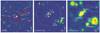 |
Fig. 1. Galaxy group and its environment. Left: galaxies belonging to the same structure (see Sect. 3.1) as the galaxies embedded in the z ≈ 1.31 Mg II nebula (shown as the red square) are indicated by white squares. The velocity relative to the most massive galaxy of the group (galaxy A, see middle panel) is indicated for each galaxy in km s−1. The structure spans ≈2 Mpc in projection and the galaxies appear well aligned. A ≈1 Mpc substructure extending beyond the MUSE Deep Field (big black dashed square) is also indicated. The MXDF and udf-10 fields are shown with the solid circle and small dashed square, respectively. The background image is an MPG(ESO2.2m)/WFI image (Hildebrandt et al. 2006). Middle: zoom-in window of (12 |


For the rest of the paper, we only focus on the subgroup of five galaxies located at the center of the larger structure (area within the red square in the first panel of Fig. 1 and shown in the two other panels) because they are the galaxies embedded in the newly detected Mg II nebula. For the purposes of clarity, the five galaxies are designated by letters1, where galaxy A is the most massive one (see Sect. 3.2). The other letters (from B to E) are attributed to galaxies depending on their projected distance to galaxy A (from the closest to the furthest, see middle panel of Fig. 1). We note that galaxy B has a lower redshift confidence level (ZCONF = 1) than the other group members in the MUSE UDF catalog (Bacon et al., in prep.). Based on a careful analysis of the [O II] NB image (see Sect. 5.1) – where [O II] emission is clearly detected at the position of galaxy B when setting low flux cuts – and the rather well constrained photometric redshift (1.25 < zBPZ < 1.47), we are confident about the redshift of this source and therefore about its group membership.
The group members are located within ≈50 kpc in projection and 120 km s−1 in redshift space (middle and right panels of Fig. 1). The projected distances and velocity offsets from galaxy A are (9 kpc, +43 km s−1), (13 kpc, −76 km s−1), (37 kpc, +2 km s−1), and (41 kpc, +43 km s−1) for galaxies B, C, D, and E, respectively (see right panel of Fig. 1 and Table 1). Galaxies B and C are aligned with the major axis of galaxy A. Similarly, galaxy D is aligned with the major axis of galaxy E.
Physical properties of the five group members.
A virial mass of ≈1011 M⊙ was estimated from the velocity dispersion of the five members using the gapper method (Beers et al. 1990; Cucciati et al. 2010; Abril-Melgarejo et al. 2021). The dynamical halo mass becomes ≈1012.3 M⊙ when considering the 14 galaxies of the larger structure. The corresponding virial radius is ≈50 kpc (Eq. (1) of Lemaux et al. 2012) for the five-member group (≈150 kpc when considering the whole structure). Alternatively, using the stellar to halo mass relation from Behroozi et al. (2019) at the redshift of the group, we calculated a DM halo mass of 1011.5 M⊙ for the central galaxy A (with 0.3 dex of uncertainties) and a virial radius of ≈90 kpc. Those two methods therefore indicate that the five group members reside inside the virial radius of the group and galaxy A.
Galaxy A is also the brightest galaxy of the larger structure in the UDF (≈24.5 mag in the F775W filter) and therefore corresponds to the dominant “brightest group galaxy” (BGG) near the halo center where the Xray intensity peak tracing the IGrM is usually observed in Xray studies (Oppenheimer et al. 2021). The BGGs have been found to have disk-like morphologies (Moffett et al. 2016), which seems to be the case for galaxy A given its elongated shape (Sect. 3.2). We note that one galaxy located at ≈1 Mpc outside the MUSE deep field and at the outskirt of the detected structure is brighter (≈23 mag in the F775W filter), with a stellar mass of ≈1010.6 M⊙ (Urrutia et al. 2019).
The middle panel of Fig. 1 shows the F775W HST/ACS image of the group and its close environment in a ≈100 × 100 kpc2 ( ) window. The known photometric redshift ranges (BPZ) from the Rafelski et al. (2015) catalog are indicated for objects without MUSE spetroscopic redshifts. Galaxies with MUSE redshifts (Bacon et al., in prep.; see also Inami et al. 2017) are shown as solid or dotted black circles, depending on the redshift confidence level (middle and right panels of Fig. 1). The systemic redshifts of the five group members have been measured for this analysis in Sect. 3.3.
A bright background galaxy (mAB, F775W = 23.4), referred to as “BKG”, spectroscopically confirmed to be at z ≈ 1.8463 (MUSE ID #18 in Inami et al. 2017) is located at an impact parameter of 2 2 (or 19 kpc) from galaxy D, i.e., within the virial radius of galaxy A. This galaxy produces a strong continuum in the MUSE data and thus appears like an interesting sight line for the analysis of the Mg II nebula (see Sect. 4.2) in absorption. No other background projected neighbors, inside a 200 kpc radius around galaxy A, have strong enough detected continua in the MUSE data to allow the detection of absorption features.
3.2. Global properties of the galaxies
The stellar masses and star formation rates (SFR) of the group members were estimated by fitting their spectral energy distribution (SED) from HST photometry (F225W, F275W, F336W, F435W, F606W, F775W, F850LP, F105W, F125W, F140W, F160W, Rafelski et al. 2015) using MAGPHYS (da Cunha et al. 2008, 2015). This version of MAGPHYS uses a Chabrier (2003) initial mass function (IMF), Bruzual & Charlot (2003) stellar models and Charlot & Fall (2000) dust attenuation. Moreover, the star formation histories (SFH) are considered exponential with random bursts superimposed. The resulting properties of the group members are given in Table 1. With a highest stellar mass of  , the galaxies of this group are rather low-mass objects. This is in contrast with previous studies where the systems embedded in ionized nebulae usually host several galaxies with stellar masses higher than 1010 M⊙ (e.g., Epinat et al. 2018; Helton et al. 2021). Despite the high uncertainties on the SFR values of the less massive galaxies as well as the few constraints on the so-called “star formation main sequence” for low-mass galaxies at z = 1.3, the five galaxies can be considered as normal star forming galaxies (Whitaker et al. 2014; Boogaard et al. 2018).
The two most massive galaxies (A and E) are seen edge-on with projected axis ratios of q = 0.329 ± 0.005 and q = 0.247 ± 0.015, respectively (corresponding to inclinations of 71 and 76°, respectively, when considering a flat disk model) and a similar position angle PA ≃ −27° (measurements from van der Wel et al. 2012 in the WFC3/F105W band, see Table 1). The three other galaxies have rounder shapes with q ≳ 0.7 and smaller sizes.
Regarding possible AGN contamination, we refer to Feltre et al. (2018, their Sect. 3.3). By cross-matching their Mg II sample (which includes four out of five of our group members) with the 7 Ms Source Catalogs of the Chandra Deep Field South Survey (Luo et al. 2017), the authors found an X-ray counterpart for only one source, which is not one of the galaxies analyzed in this paper. We do not find any X-ray counterpart for galaxy B (not in Feltre et al. 2018). The faintness and low stellar masses of the galaxies (Table 1), the reasonable line widths, and the lack of typical AGN lines such as C II] λ3425, also indicate that the presence of an AGN in those galaxies is unlikely. Nonetheless, the presence of low luminosity or heavily obscured AGN cannot be entirely excluded.
3.3. Integrated spectra
Figure 2 displays a zoom-in HST/ACS view in the F775W filter (first column) and the integrated spectrum (second column) of each group member. We display the ODHIN spectrum (see Sect. 2), which makes use of the higher spatial resolution of the HST images to perform a deblending of sources in the MUSE cubes. The deblending feature of the ODHIN software is particularly needed here as the emission from the [A,B,C] and [D,E] galaxies are overlapping at MUSE resolution (see Fig. 3a). The corresponding integrated error spectra are shown in gray in each panel and errors are directly indicated on the spectra (in gray) in the insets.
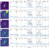 |
Fig. 2. Integrated spectra of the five group members. Left: 2″ × 2″ HST/ACS F775W images of the five group members. The central white cross and contour indicate the HST coordinates and segmentation map from Rafelski et al. (2015). Right: integrated spectrum (units of 10−20 erg s−1 cm−2 Å−1) of the galaxy shown in the corresponding left panel extracted within the HST segmentation map contour using the ODHIN software (Bacher 2017, see Sect. 3.3) and smoothed with a 7 Å FWHM Gaussian function. The positions of several emission (absorption) lines are indicated by vertical dotted green (red) lines. The gray unsmoothed spectra show the 1σ uncertainties which have been offset for readability. The unsmoothed Mg II and [O II] lines (vertical dashed lines) are shown in the insets. The vertical blue shaded areas indicate the spectral widths used to construct the Mg II NB image shown in Fig. 3a. |
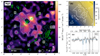 |
Fig. 3. Metal-enriched intragroup medium revealed by MUSE. (a) Mg II narrow-band image of the group (see Sect. 4.1) smoothed with a 0.6″ FWHM Gaussian and plotted with a power-law stretch. The white contours correspond to Mg II significance levels of 1.5, 2 and 3σ (solid, dashed, and dotted, respectively) where 1σ corresponds to a SB level of 1 × 10⁻¹⁹ erg s−1 cm−2 arcsec−2. The blue contours indicate the negative SB values (same coding as the positive contours) corresponding to the absorbing regions (see Sect. 4.2). The green contours trace the continuum of the group members close to Mg II and the neighboring galaxies as detected in the HST/ACS F775W image. The dotted green contour corresponds to the outer HST continuum contours of the group members set at the MUSE resolution. The FWHM of the MUSE PSF and smoothing kernel are shown with a hatched and empty circle, respectively, at the bottom-right of the figure. (b) Exposure map centered on the group. The solid, dashed, and dotted black contours indicate 10, 30, and 90 h depth, respectively. The white contour corresponds to the Mg II significance level of 1.5σ. (c) Mg II absorption in the spectrum of the background galaxy BKG located at an impact parameter of 19 kpc from galaxy D in projection and at the nebula redshift. The blue line is the best-fit model of the Mg II doublet absorption (Sect. 4.2). The 1σ uncertainties are shown in gray and the hatched areas indicate the position of strong sky lines and noise peaks. The systemic redshift of galaxy D is indicated by vertical dashed lines. |
The systemic redshifts of the group members are calculated from those spectra by fitting the [O II] doublet, which is the line with the highest signal-to-noise ratio (S/N) for all sources. We fit the doublet using two Gaussian functions with fixed peak separation and considering the variance of the MUSE cube. The errors on the fit parameters are estimated using bootstrapping; 1000 realizations of the line doublet are generated using the error spectrum assuming that the errors are normally distributed around the observed flux values. The resulting errors on the systemic redshift measurements (given in Table 1) are on the order of 10−5.
All the galaxies show a stellar continuum with clear [O II] and Mg II emission (see inset panels in Fig. 2). We note that both Mg II and [O II] doublets are impacted by significant skylines. The spectrum of the most massive galaxy (A) displays other emission lines like [Ne III], H8, Hϵ as well as C II] λ2326 and [O II] λλ2470, 2471. Moreover, the Balmer absorption is detected on the red side of the [O II] line. The Mg II line of galaxy A shows a P-Cygni profile and a detection of the Mg Iλ2852 absorption line. At the redshift of the group, the UV transitions Fe II* (λ2365, λ2396, λ2612, λ2626) are observable with MUSE; most of the corresponding emission and absorption lines are detected in the spectrum of galaxy A (top-right panel of Fig. 2). Using the shallower mosaic and udf-10 MUSE datacubes, Feltre et al. (2018) and Finley et al. (2017) respectively studied the Mg II and Fe II* emission of star-forming galaxies. Both studies classified the Mg II doublet of galaxy A as a P-Cygni profile. In Feltre et al. (2018), galaxy C is classified as an Mg II emitter and galaxy E as a non-detection. The redshift confidence level of galaxy D was not high enough to be included in their sample and, as mentioned before, galaxy B is a newly detected galaxy that was not in their sample either.
The Mg II rest frame equivalent widths (EW) of the Mg IIλ2796 line calculated using pyplatefit in Bacon et al. (in prep., see also Bacon et al. 2021) are given in Table 1. The Pyplatefit software performs a stellar continuum fit using a simple population model (Brinchmann et al. 2013) and fits the emission and absorption lines after subtracting the continuum. The intrinsic Mg IIλλ2796,2803 absorption in the spectra of O/B stars is expected to be very weak (≈0.6 Å for population ages up to a few 100 Myr, Henry et al. 2018) and therefore cannot explain the observed absorption. The Mg II absorption is most likely dominated by continuum photons pumping by Mg+ ions along the line of sight, followed by isotropic re-emission out of line of sight, as a result of resonant scattering. This leads to a net absorption in front of the continuum sources, and possibly large-scale diffuse emission that fills the absorption troughs. This effect is called emission infill (e.g., Prochaska et al. 2011; Scarlata & Panagia 2015; Zhu et al. 2015; Finley et al. 2017). The EW values reported in Table 1 are not corrected for this effect. We also did not attempt to correct our Mg II observations for emission infill, nor the spectra or the narrow bands (Sect. 4.1) because it would inevitably imply an astrophysical assumption that absorbing and emitting regions are spatially different and can be separated. Since the physical meaning of any simple correction is limited, we present the full complexity of these Mg II data and highlight the novelty of the detection of such diffuse large-scale structures. Our non-corrected measurements enable (i) direct and simple comparisons with other studies in terms of detection limits, observed flux, and spatial variations, as well as (ii) the reproducibility of our results and measurements. Finally, we note that the absorption correction has an effect at galaxy scale only, so our conclusions about the large scale intragroup medium are not impacted by the non-correction.
In summary, we are looking at a compact group of five low-mass members located at the center of a larger structure at high redshift. Taking advantage of the deep MXDF data, we analyzed the Mg II properties of the IGrM in the next section (Sect. 4) and its [O II] and Fe II* properties in Sect. 5.
4. Mg II intragroup nebula
4.1. Mg II narrow-band image
The Mg II structure was extracted in a subcube of  (≈100 × 100 kpc2 at z ≃ 1.31) centered on the coordinates RA = 53°09′25″, Dec = −27°46′44″. We estimated the continuum by performing a spectral median filtering on the subcube using a wide spectral window of 200 spectral pixels (250 Å). After subtracting this continuum-only cube from the original one, we obtained an emission lines-only cube, from which we optimally created the Mg II NB image of the group as follows.
In order to encompass all the Mg II emitting flux from the five galaxies of the group while limiting the noise, we adopted the following method: (i) the Mg II line is extracted by integrating inside a circular aperture including the five group members, centered on the continuum-subtracted subcube, which maximizes the integrated flux of the Mg IIλ2796 line (r = 3.2″), (ii) the NB image of the λ2796 Mg II line is created by summing the continuum-subtracted subcube over the wavelength range 6445.0−6453.75 Å (≈400 km s−1) delimiting the line; the borders of the line are determined by wavelengths for which the flux reaches zero. The same procedure is applied to extract the λ2803 line of the Mg II doublet (6462.5−6468.75 Å, ≈290 km s−1). The total Mg II emission NB image is finally obtained by adding the λ2796 and λ2803 NB images. A broader band Mg II image is presented in Fig. C.1 and confirms that our method provides an S/N-optimized NB image without missing flux (see the residuals image in the right panel of Fig. C.1).
The NB image shown in Fig. 3a has been smoothed using a  (3 MUSE spaxels) FWHM Gaussian in order to increase the S/N while keeping the spatial resolution as good as possible (PSF of 0.52″ FWHM, see Fig. B.1). The 1σ significance level corresponds to a surface brightness (SB) of 1 × 10⁻¹⁹ erg s−1 cm−2 arcsec−2. As shown in Fig. 3b, the exposure time ranges from ≈30 to 90 h through the Mg II nebula (white contour). This explains the noisier regions in the upper right corner of the NB image. As a consequence, we refrain from estimating the noise from empty regions around the nebula to compute the limiting SB contours and use the propagated variance of the MUSE cube in each pixel after smoothing. The total Mg II flux within 2σ significance level is 7.48 ± 0.50 × 10⁻¹⁸ erg s−1 cm−2 and corresponds to a total luminosity of 8.0 ± 0.5 × 1040 erg s−1 without dust correction.
The eight 1.25 Å slices (from −177 to +286 km s−1) of the MUSE subcube are summed to create the λ2796 Mg II NB image are shown in Fig. 4. We note that because of the line spread function, those slice images are somewhat correlated. In spite of this, the spatial variations are still visible between adjacent slices (see Sect. 4.4).
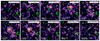 |
Fig. 4. Channel maps around the Mg IIλ2796 emission. Each map corresponds to one MUSE subcube slice (1.25 Å or 58 km s−1 at the redshift of the group). The velocity window relative to the systemic redshift of galaxy A is indicated on each panel. Contours are the same as in Fig. 3a. The eight central slices (from −177 to +286 km s−1) are summed to create the optimized λ2796 Mg II NB image shown in Fig. 3a (see Sect. 4.1). |
4.2. Mg II morphology
Figure 3a shows the extended nature of the Mg II emission around this group of five galaxies. The observed nebula encompasses a projected area of 15 arcsec2, corresponding to 1000 kpc2 at the redshift of the group, above the 2σ SB threshold of 2 × 10⁻¹⁹ erg s−1 cm−2 arcsec−2. The detected nebula resides within the virial radius of galaxy A (Sect. 3.1) and has an elongated shape linking the five group members with maximal projected extent reaching ≈70 kpc along the A/E direction and ≈40 kpc along the B/C direction.
The strongest Mg II emission coincides spatially with galaxy C. Another emission peak is observed in between galaxies A and B. While globally the nebula appears aligned with the minor axis of galaxie(s) A (and E) as expected e.g., in a scenario where Mg II is emitted by biconical outflows launched perpendicular to the galaxy disk (Bouché et al. 2012), here the two intensity peaks are aligned with the major axis of the most massive galaxy A. This point is discussed in Sect. 6.2.
The 2D map reveals a lack of flux at the positions of galaxies A and BKG (background galaxy). Those features are artificially created by the continuum subtraction procedure (see Sect. 4.1): the absorption features appear negative once the continuum has been subtracted. The fact that Mg II in emission is observed at the position of galaxy A in the [+54; +112] and [+112; +170] km s−1 channel maps of Mg IIλ2796 (Fig. 4) indicates that both absorption and emission coexist in this region. The lack of flux detected at the position of galaxy A in the summed NB image (Fig. 3a) therefore corresponds to regions where the absorption is dominant over the emission. As indicated in Sect. 3.3, our study is not aimed at obtaining a correction for the emission infill effects here because our study focuses on the larger scale Mg II nebula.
Interestingly, while Mg II emission lines are detected in the integrated spectra of the galaxies D and E, the Mg II map shows no flux at the location of galaxy E and offset emission near galaxy D. This can be caused by the galaxy’s absorption being completely filled by the emission (e.g., Zabl et al. 2021). The spectra of the galaxies D and E indeed show hints of low S/N absorption lines, which are within the Mg II NB spectral bandwidth (see Fig. 2). We also note that the segmentation map of galaxy D extends beyond the stellar body of the galaxy (Fig. 2). This implies that the Mg II emission observed in the spectrum of galaxy D likely originates from circumgalactic regions (as seen in the Mg II map in Fig. 3a).
The ODHIN spectrum of BKG (z ≃ 1.8463, see Fig. 1c), which is located outside the detected Mg II emission nebula and at a projected distance of 19 kpc from galaxy D, shows Mg II absorption at the same redshift as the nebula (see Fig. 3c). Such a detection indicates that the Mg II gas even extends beyond the detected Mg II emission nebula. Using the line fitting procedure described in Sect. 3.3, we measured an Mg IIλ2796 rest frame EW of 0.5 Å for the absorption. This measurement falls well on the Mg II EW versus impact parameter relation found in several absorption studies (e.g., Lundgren et al. 2021). Using the Ménard & Chelouche (2009) relation between the H I column density and the rest frame Mg IIλ2796 EW we obtained the rough estimate of 1019 atoms cm−2 for the extended gas column density in this line of sight.
The spatially resolved MUSE view of the nebula also reveals that the Mg II distribution is different from that of the continuum: the Mg II gas is more extended than the stellar content of the galaxies (see Sect. 4.3) and a projected bridge seems to link galaxy subgroups [A,B,C] and [D,E] (see Sect. 4.3). This bridge might not be a projection effect because of its tentative detection (S/N ≲ 2) in the single 1.25 Å (58 km s−1) cube slice between +54 and +112 km s−1 relative to the systemic redshift of galaxy A (bottom left panel of Fig. 4). We can also mention that the Mg II spatial distribution is not homogeneous in between the galaxies: several intensity peaks are detected at S/N > 3. They suggest the presence of gas clumps or satellite galaxies (undetected in the HST and MUSE data) residing in the IGrM (see discussion in Sect. 6.2.1).
4.3. Radial Mg II surface brightness profile
In order to highlight the extended nature of the Mg II emission around and in between the galaxy group members, we computed azimuthally averaged radial surface brightness profiles of the Mg II and continuum emission centered on galaxy A (Fig. 5, first panel). The Mg II profile (blue) is measured on the unsmoothed Mg II NB image (Sect. 4.1) after masking pixels located outside an ellipse corresponding to the 1σ significance level in order to increase the S/N in the two-pixel-wide annuli (or truncated annuli) used for the aperture photometry (see inset panels). The width of the annuli (0.4″) is comparable to the spatial resolution element of the data (PSF FWHM of 0.52″).
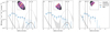 |
Fig. 5. Azimuthally averaged radial surface brightness profile of the Mg II nebula centered on galaxy A (blue data points). For comparison the profile of the Mg II continuum (±20 000 km s−1 around the Mg II doublet) shown in black is also rescaled (gray) to the Mg II SB at the location of galaxy C (where Mg II absorption is unlikely, see Appendix D). The positions of the group members are indicated with vertical dashed lines. The radial profiles have been calculated using unsmoothed Mg II and continuum images after masking the pixels outside the 1σ significance level approximated with an elliptical contour as shown in the inset (left). Middle and right panels: radial profiles after masking the pixels above and below the [A,B,C] axis, respectively. In the insets, we also show the two-pixel annuli used to construct the profiles as white circles. |
The Mg II continuum radial SB profile (black) is measured from a continuum image extracted from the continuum-only cube within a window of ±20 000 km s−1 around the Mg II doublet. This broad spectral window does not include strong absorption or emission lines and ensures a good enough S/N. The neighboring sources were rigorously masked in order to avoid contamination and the same elliptical mask used on the Mg II image was applied to compute the continuum SB profile. Errors were measured in each (truncated) annulus using the estimated variance from the MUSE data cube. To aid the visual comparison, the continuum profile has been rescaled to the Mg II SB at the position of galaxy C, which is where the brightest Mg II intensity peak is observed. Galaxy C is unlikely to be affected by Mg II absorption as its measured Mg II line ratio λ2796 Å/λ2803 Å is very close to two, which is the expected value for optically thin emission (see Appendix D). Moreover, no fluorescent Fe II* lines are significantly detected for galaxy C which is in good agreement with no infilling effect and therefore no absorption (see Appendix D, Mauerhofer et al. 2021).
The Mg II SB profile appears more extended than the continuum, especially in between the galaxies [A,B,C] and [D,E] – radial positions are indicated by vertical dashed lines – where a low SB projected “bridge” at ≈2 × 10⁻¹⁹ erg s−1 cm−2 arcsec−2 level can be identified. In order to differentiate between the extended emission around the galaxy subgroup [A,B,C] and in between the galaxy subgroups [A,B,C] and [D,E], we compute the radial SB profiles above and below the [A,B,C] axis (see insets for illustration) in the middle and right panels of Fig. 5, respectively. The Mg II emission appears more extended than the rescaled continuum in both directions (above and below the [A,B,C] axis), confirming the detection of diffuse Mg II emission around the group members as well as a low SB Mg II bridge (≈2 × 10⁻¹⁹ erg s−1 cm−2 arcsec−2) detected with more than 1.5σ significance spanning ≈50 kpc in projection between the galaxy subgroups [A,B,C] and [D,E] (see Fig. 3a). We go further into the analysis of the Mg II nebula in the next section by looking at the spatial variation of the spectral properties of Mg II.
4.4. Spatially resolved Mg II properties
The kinematics of the gas connecting the galaxy group can provide crucial information on its nature and origin. To reveal the spatial variations of the Mg II spectral profile within the nebula, we built a 2D binned map using the weighted Voronoi tesselation method (Cappellari & Copin 2003; Diehl & Statler 2006). This method allows us to increase the S/N in the surroundings of the galaxies where the surface brightness is the lowest. The binning was performed on the Mg II NB image constructed from the MXDF datacube (see Sect. 4.1), for which the pixels with S/N < 1.5 (corresponding to the outer SB contour in Fig. 3a) have been masked in order to remove the noise-dominated pixels. The resulting binned Mg II map consists of 20 bins with S/N > 3 and probes the detected Mg II nebula above ≈2 × 10⁻¹⁹ erg s−1 cm−2 arcsec−2.
The spectral extraction is performed from the MUSE continuum-subtracted cube smoothed with a 0.6″ FWHM Gaussian in order to increase the S/N while keeping a good spatial resolution (see Appendix B). We extracted the Mg II doublet in each resulting bin and measured the properties of the emission lines by modeling the doublet as a sum of two Gaussian profiles with a fixed peak separation.
The errors on the line parameters (peak position and FWHM) were estimated using bootstrapping. For each segmented area, we generated 1000 realizations of the extracted line where each pixel is randomly drawn from a normal distribution centered on the original pixel value and with standard deviation derived from the estimated noise value. The noise of each extracted spectrum corresponds to the standard deviation of the data measured in two 200 Å wide spectral windows located on each side of the Mg II doublet. We note that due to smoothing as well as the PSF, the line parameters between neighboring pixels are somewhat correlated. However, the spatial variations are still visible.
Figure 6 (top left panel) shows the resolved map of the Mg IIλ2796 peak position relative to the systemic redshift of galaxy A. The observed Mg II velocity gradient suggests an overall rotation of the structure along the major axis of galaxy A consistent with an extension of the ISM rotation (as probed by the [O II] emission, see Sect. 5.1) at the CGM scale within which the satellite galaxies B and C are embedded. This ISM/CGM co-rotation is also observed in simulations and observations (e.g., Smith et al. 2019; Zabl et al. 2019, 2021; Ho et al. 2020; Tejos et al. 2021).
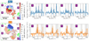 |
Fig. 6. Spatially resolved Mg II and [O II] properties. Left: binned line-of-sight velocity maps of the Mg II (top) and [O II] (bottom) emission relative to the systemic redshift of galaxy A (Sects. 4.4 and 5.1). The black contours correspond to the 1.5σ significance level. The green contours trace the galaxies detected in the HST/ACS F775W image. The FWHM of the MUSE PSF and smoothing kernel are shown with a hatched and an empty circle, respectively, at the top right of the panels. The diverging Mg II and [O II] colormaps are centered on the systemic redshift of galaxy A and have the same dynamical range to ease the visual comparison (Sect. 5.1). Right: Mg II (top) and [O II] (bottom panels) doublet extracted in the elliptical areas traced in purple and designated by the same number on the map (left panels). The vertical dashed lines correspond to the systemic redshift of galaxy A. The vertical hatched bands indicate the presence of sky lines. |
The top-right panels of Fig. 6 show the unsmoothed Mg II doublet extracted in the elliptical areas traced in purple and designated by the same number on the map. These apertures are independent of the Voronoi bins and aim to show the Mg II line profile in some diffuse regions of the nebula. The velocity variations are small (< 50 km s−1) in the diffuse regions.
The kinematics of the nebula appear to be overall shifted towards higher velocities (by +50 km s−1 on average) compared to the [O II] emission (bottom left panel, see Sect. 5.1). The highest velocity variations are observed along the minor axis of galaxy A and reach ≈+120 km s−1 and −80 km s−1 with respect to the systemic redshift of galaxy A. As discussed in Sect. 6.2.1), this supports the presence of an outflow emerging from galaxy A.
5. [O II] and Fe II* emission
At the redshift of the group, MUSE covers the non-resonant collisionally excited [O II] doublet and the fluorescent Fe II* lines. The corresponding NB images and radial SB profiles are shown in Fig. 7 and are created following the same procedure as for the Mg II emission (Sects. 4.1 and 4.3, respectively).
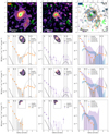 |
Fig. 7. [O II] and Fe II* spatial properties. First column: [O II] NB image (top, Sect. 5.1). Legend is the same as in Fig. 3a. The 1σ level corresponds to a SB of 2.5 × 10⁻¹⁹ erg s−1 cm−2 arcsec−2. Bottom panels: total and directional (below and above the [A,B,C] axis) azimuthally averaged radial SB profiles centered on galaxy A (from top to bottom, respectively, see also insets for illustration) of the [O II], [O II] continuum and rescaled [O II] continuum (orange, black and gray, respectively) emission. The radial positions of other group members with respect to galaxy A are indicated by the vertical dashed lines. Second column: same as first column but for Fe II* (purple). Third column: comparison of the Mg II, [O II] and Fe II* 2σ significance level contours (blue, orange, and purple, respectively) superimposed on the Mg II NB image (top). Bottom panels: show a comparison of the radial SB profiles where the Fe II* profile (shaded purple) has been rescaled to the [O II] profile at the SB peak and Mg II (shaded blue) at the position of galaxy C (Appendix D). For this plot the [O II] map was degraded to the resolution of the Mg II emission (Sect. 5.1). |
5.1. Low-surface-brightness [O II] nebula
The [O II] NB map (Fig. 7, top left) is obtained by summing the continuum-subtracted cube in the wavelength range [8590, 8605] Å (≈500 km s−1). In order to improve the S/N, the image was smoothed using a  FWHM Gaussian function. The white contours correspond to the 1.5, 2, and 3σ significance levels with 1σ corresponding to 2.5 × 10⁻¹⁹ erg s−1 cm−2 arcsec−2. The total [O II] flux and luminosity within the 2σ significance level contour (dashed white line) are 5.95 ± 0.07 × 10⁻¹⁷ erg s−1 cm−2 and 6.36 ± 0.07 × 1041 erg s−1, respectively.
The [O II] azimuthally averaged radial SB profiles are shown in the lower left panels of Fig. 7. The profiles are constructed following the same procedure as for Mg II (see Sect. 4.3) with an additional step for the construction of the continuum image where the cube slices within ±20 000 km s−1 polluted by skylines have been masked. This is particularly important because at the redshift of the nebula, the [O II] line falls next to many sky lines. The [O II] doublet is itself contaminated by a skyline (see vertical gray line in the lower right panels of Fig. 6) preventing us from in-depth analysis.
When comparing the [O II] and rescaled continuum radial SB profiles in Fig. 7, only one data point is above the rescaled continuum profile with more than 2σ significance. The inner profile has the same shape as the continuum one implying that the [O II] emission is not significantly more extended than the continuum inside a radius of ≈2″ from galaxy A. Extended [O II] emission at the same position as the Mg II bridge, namely, in between the galaxies [A,B,C] and [D,E], is detected with 2σ significance level in the [O II] NB image (Fig. 7, top left). However, due to averaging effects, the [O II] bridge is less significant on the radial profiles computed below the [A,B,C] axis, namely, in the direction of the [D,E] subgroup (first column third row of Fig. 7). The radial SB profile computed above the galaxies A, B and C (bottom left panel) indicates extended [O II] emission at radii > 2.5″ from galaxy A, suggesting the presence of an ionized [O II] halo around this galaxy subgroup. Comparisons of the Mg II and [O II] spatial extent and radial SB profiles are presented in Fig. 7 (top two right panels). Since the MUSE PSF is narrower at the [O II] wavelength than at the Mg II wavelength, we degraded the [O II] NB image by convolving it by a Moffat function whose parameters (a = 0.22 and b = 2.87, see Bacon et al. 2017) have been empirically determined so that the [O II] and Mg II images have the same PSF. While the [O II] and Mg II spatial distributions are consistent, the Mg II radial SB profiles (azimuthally averaged and in directions, bottom right panels) are all flatter than the [O II] profiles. This can be attributed to the resonant nature of the Mg II transition (see Sect. 6.2.2).
The binned line-of-sight velocity map of the [O II] emission is shown in the bottom left panel of Fig. 6. The map is constructed following the same procedure as for Mg II (Sect. 4.4) and consists of more bins (57) because of the higher S/N of the [O II] emission near the galaxies. At the position of the galaxies, the observed spatial variations of the [O II] peak positions are consistent with their redshift relative to galaxy A (right panel of Fig. 1). The lower right panels of Fig. 6 show the unsmoothed [O II] lines extracted in the same elliptical apertures as for Mg II (top panels). Interestingly, in region #4 the Mg II emission is stronger than [O II]. This can be explained by the resonant nature of the Mg II transition (see Sect. 6.2.2) resulting in Mg II being more extended that [O II]. The existence of the [O II] bridge is reinforced by the detection of the [O II] doublet in this area (region #3 in Fig. 6).
5.2. Extended Fe II* emission
The Fe II* NB image (top middle panel of Fig. 7) is obtained by summing the λ2365, λ2396, λ2612 and λ2626 NB images, of which the observed spectral windows are [5448.75, 5456.25], [5522.5, 5530.0], [6021.25, 6027.5], and [6041.25, 6066.25] Å, respectively. The total Fe II* flux and luminosity within the significance level contour of 2σ is 5.3 ± 0.5 × 10⁻¹⁸ erg s−1 cm−2 and 5.7 ± 0.6 × 1040 erg s−1, respectively.
Given that the Mg II and Fe II* lines are close in wavelength, we consider the same stellar continuum (see Sect. 4.1). Therefore, the radial SB profiles of the continuum (black profile in the middle bottom panels) are the same as for Mg II. The comparison between the Fe II* emission and the rescaled continuum radial SB profile reveals that the Fe II* emission is more extended than the continuum (see central panel of Fig. 7) second row. The Fe II* extended emission appears more significant in the direction of the galaxies D and E (compare the central panels of the Fig. 7 third and fourth rows). This is confirmed in the NB image where the Fe II* emission indeed extends along the minor axis of galaxy A and towards galaxy D. We discuss the origin for the extended nature of the Fe II* emission in Sect. 6.2. Contrary to Mg II and [O II] emission, the Fe II* emission does not surround the five-galaxy group but is rather centered on the most massive galaxy A (see the Mg II, [O II] and Fe II* contours and radial SB profiles comparison in the last column of Fig. 7).
Similarly, Finley et al. (2017) using MUSE found the Fe II* emission of a z = 1.29 galaxy to be more extended than the stellar continuum and aligned with the minor axis of the galaxy. The velocity gradient and shape of the Fe II* emission suggest the presence of a conical outflow. The faintness of the Fe II* emission of galaxy A hampers a kinematic analysis.
6. Discussion
6.1. Existence of an Mg-enriched intragroup medium
Historically, the existence of an intragroup medium enriched in magnesium has been suggested by absorption studies in order to explain the fact that while the strong Mg II absorbers (rest frame equivalent width EW > 0.8 Å) are generally associated with a single galaxy (within 100 kpc, e.g., Bouché et al. 2007, 2012; Ho et al. 2017; Schroetter et al. 2016, 2019; Zabl et al. 2019; Lundgren et al. 2021), sometimes weaker Mg II absorbers (EW < 1 Å, e.g., Muzahid et al. 2018; Dutta et al. 2020) or H I absorbers (e.g., Péroux et al. 2017; Rahmani et al. 2018) can be matched to groups of multiple galaxies (Δr < 500 kpc and Δv < 500 km s−1), which is in agreement with clustering studies (Bouché et al. 2006; Lundgren et al. 2009; Gauthier et al. 2009).
The question of whether observed absorption features (with EW < 1 Å) imprinted in the spectrum of a background source are tracing gas coupled to the group or circumgalactic gas of an individual galaxy is still a matter of debate. Indeed, absorption studies reported contradictory results, some suggesting that Mg II absorbing systems were associated with the CGM of the individual group members (e.g., Bordoloi et al. 2011; Fossati et al. 2019) and others to a widespread IGrM (e.g., Bielby et al. 2017; Péroux et al. 2017; Nielsen et al. 2018) originating from a mixture of previous tidal interactions between group members and outflowing winds. Disentangling the two is very challenging, especially when there is only one-dimensional information for a given system.
Our discovery of the first extended Mg II nebula surrounding and connecting the members of a five-galaxy group provides a panoramic view of the neutral enriched gas residing in between galaxies. This group is rather small and compact (see Sect. 3.1), meaning that it is likely an interacting system where the CGM of individual galaxies are mixed. This idea is reinforced by the fact that the detected Mg II nebula resides inside the virial radius of galaxy A estimated at ≈100 kpc. Moreover, the detection of a gaseous bridge in between the two subgroups [A,B,C] and [D,E] suggests that we are observing a widespread low-surface-brightness structure embracing the five galaxies, also called the “intragroup” medium. We note that there is no precise definition of the IGrM in the literature. Our analysis brings the first observational evidence of a low SB diffuse component of neutral gas residing within a galaxy group at z > 1 that we define as the intragroup medium.
The detection of Mg II absorption in the spectrum of the background source BKG (see Sect. 4.2) indicates that the IGrM is actually even more extended than the detected nebula. Our EW measurement of the Mg II absorption (Sect. 4.2) is in good agreement with the EW versus impact parameter relation established by quasar absorption line studies (e.g., Lundgren et al. 2021). This result highlights the complementarity of the absorption and emission methods to study the gas around galaxies.
6.2. Origin of the intragroup nebula
In this section, we discuss two points: the presence of enriched gas beyond the galaxies and the mechanisms that make it shine.
6.2.1. Reasons for the presence of enriched gas so far from the stars
Several scenarios have been suggested to explain the presence of magnesium-enriched gas in between the galaxies of a group. Magnesium atoms are α elements released in the ISM and CGM by core collapse supernovae. One can therefore naturally imagine that the magnesium gas residing outside galaxies has been ejected through strong supernovae-driven outflows. The P Cygni shape of the Mg II doublet in the integrated spectrum of galaxy A (see Fig. 2 top) is in good agreement with this scenario. Indeed, according to radiative transfer (RT) models, this line profile is a signature of resonant scattering in an optically thick outflowing medium where the redshifted emission corresponds to back-scattered photons reflected by the receding medium (Haiman et al. 2000; Dijkstra et al. 2006; Verhamme et al. 2006; Kollmeier et al. 2010). The Mg II lines of galaxies D and E seem to be redshifted compared to their systemic redshifts (Fig. 2), however, the continuum is too faint to detect significant absorption lines and, thus, too faint to detect the P Cygni profiles, namely, the presence of outflows for those galaxies. We detected > 2σ Mg II emission aligned with the minor axis of galaxy E and near galaxy D (Fig. 3). These regions could have been enriched via outflows after supernovae feedback. However, the S/N of our data is too poor in these areas to carry out a resolved kinematics study. The resolved Mg II map (Fig. 6) shows that the two regions along the minor axis of galaxy A have different velocities with opposite signs (≈ + 120 and −80 km s−1 with respect to the systemic redshift of galaxy A), providing additional evidence of the presence of an outflow. Even if we do not eventually find clear evidence of an outflow in the four other galaxies, we cannot exclude the deposition of metals in the CGM by past feedback processes explaining the observed diffuse Mg II emission detected around each of the galaxy members. In that scenario, we could imagine that the low-surface-brightness gaseous bridge in-between the galaxy subgroups [A,B,C] and [D,E] could be due to galactic wind transfer between the group members as observed in the FIRE simulation (Anglés-Alcázar et al. 2017).
The proximity of the galaxies, as well as the detection of a bridge in-between the galaxy subgroups is also compatible with another scenario where the magnesium gas has been tidally stripped out of galaxies due to past gravitational interactions among the galaxy group members. In this framework, the detected enriched bridge would correspond to a tidal feature linking the galaxies. In this scenario, Bielby et al. (2017) suggested that the IGrM could consist of multiple cool gas systems orbiting around galaxies to form the IGrM. As mentioned in Sect. 4.2, we detect several S/N > 3 Mg II intensity peaks within the IGrM, which, if real, could be associated with the cool gas clouds described in Bielby et al. (2017). According to hydrodynamical simulations, such cold clumps could originate from gas density perturbations after tidal interactions (Nelson et al. 2020). As mentioned above, we could also argue that the gas in the bridge could be outflowing material from galaxy A undergoing an “intergalactic transfer” to galaxy D (Anglés-Alcázar et al. 2017). However, neither the fluorescent Fe II*, nor the non-resonant [O II] emission are symmetrically distributed around galaxy A; rather they extend preferentially towards galaxy D and E (see top panels of Fig. 7), suggesting that the enriched gas detected in the bridge has been stripped of galaxies by tidal or ram pressure forces. Moreover, we do not observe any strong velocity gradients in the bridge, indicating that the bridge dynamics are consistent with the rest of the structure (left panel of Fig. 6) and reinforcing the presence of tidally disrupted material. It is, however, more difficult to disentangle the different scenarios in the close surroundings of the galaxies where – given the very small physical separation between the sources – outflows, tidal interactions, and intergalactic transfer could play a role.
Given the proximity of the five group members, we suggest that past tidal interactions are likely the dominant mechanisms explaining the presence of magnesium-enriched gas in the IGrM. Plenty of cool stripped gas is actually observed in simulations in the form of tidal features (e.g., Rosdahl & Blaizot 2012; Nelson et al. 2020). In Rosdahl & Blaizot (2012), the ≈1011.5 M⊙ DM halo (similar to our system) at z = 3 indeed shows orbiting satellites and tidal tails. Such H I tidally disruptive material is also observable in the local Universe, namely, in between the galaxies of the M 81 system (Yun et al. 1994).
6.2.2. Possible mechanisms behind the shine of the intragroup magnesium gas
Several mechanisms can explain the emission of Mg II photons from the intragroup gas. The possible sources, which can arise at all scales (ISM, CGM, IGrM), are as follows:
Stellar continuum at λ∼ 2800Å. By summing the continuum contribution of the five galaxies in the group, we estimate the Mg II photon budget from the stellar continuum to 9.0 ± 1.0 × 10⁻¹⁸ erg s−1 cm−2 corresponding to a total luminosity of 9.6 ± 1.1 × 1040 erg s−1 without dust correction and considering the sum of the two doublet lines (see Sect. 4.1).
Photo-ionization by Mg II ionizing radiation (λ < 825 Å), from the stellar continuum of galaxies in the group or from the UV background (UVB) and collisional ionization of Mg+ ions into Mg2+ ions, followed by recombination cascades leading to the emission of nebular Mg II photons. Using Cloudy photo-ionization models, we estimate the nebular Mg II photon budget corresponding to collisions and photo-ionization from the stellar continuum (see Appendix E).
Mg II photons produced by shocks resulting from gravitational interactions or galactic outflows from galaxies.
The Mg II doublet is a resonant line meaning that the Mg II photons are likely to be scattered within an Mg+ gas cloud. This property is usually invoked to explain the diffuse resonant emission around galaxies, namely, Lyα halos (e.g., Kusakabe et al. 2019; Leclercq et al. 2020). However, this process erases the information on the location where the photons have been emitted. In the following, we discuss the possible distributions of sources and mechanisms that can explain the intragroup Mg II luminosity, and light distribution.
Central source with scattering. Stellar continuum: the first possibility to explain extended Mg II emission is the scattering of stellar continuum photons, namely, the re-emission of continuum photons absorbed in the Mg II transition. While Wisotzki et al. (in prep.) found that this process is likely the dominant one in their system, Zabl et al. (2021) found that it is (under the assumption of a biconical outflow) not likely enough to explain the brightness of the Mg II halo. In the group studied here, the Mg II continuum luminosity (9.6 ± 1.1 × 1040 erg s−1 without dust correction and integrating over the same velocity range as the Mg II NB image, see Sect. 4.1) is enough to explain the observed Mg II nebula (total luminosity of 8.0 ± 0.5 × 1040 erg s−1). This suggests that the continuum scattering scenario is an important process at play in this system.
Nebular emission: Diffuse Mg II emission can also be produced by the scattering of nebular Mg II photons produced in the ISM of galaxies. For this mechanism, the Mg II photons are produced by collisions and recombinations associated with stellar UV radiation in star-forming regions of galaxies. The escaping photons can then scatter into the surrounding Mg+ gas and some are redirected towards the observer. We used Cloudy models (Ferland et al. 2017) to estimate the intrinsic Mg II flux budget produced by the stars of the five galaxy group members. We found an intrinsic Mg II/[O II] flux ratio varying between ∼10 and 30% (see Appendix E for more details). The total observed Mg II/[O II] flux ratio of the nebula (12%) being lower than the intrinsic one, or similar depending on the models, we conclude that there is enough nebular Mg II emission to explain the observed Mg II extended emission through resonant scattering of photons originally produced in H II regions. This scenario is reinforced by the spectral shapes of the galaxies (i.e., P Cygni and redshifted lines with respect to the systemic redshift), suggesting that Mg II photons scattered in an outflowing medium (see Sect. 6.2.1).
In situ emission. Collisions + photo-ionization: another scenario to explain the extended Mg II emission is that enough Mg II ionizing photons (λ0 < 825 Å) escape the ISM of galaxies – perhaps facilitated by galaxy-scale outflows – so that Mg II photons are produced through photo-ionization in situ, that is, directly in the CGM or IGrM. It is however well known that the escape of ionizing photons from galaxies is very low (e.g., Malkan et al. 2003; Bridge et al. 2010; Rutkowski et al. 2016; Alavi et al. 2020). The spatial coincidence of the Mg II and the non-resonant collisionally excited [O II] emission lines support this “non-scattering” origin. We note that the resulting Mg II photons can then scatter in the surrounding magnesium located in the IGrM, as in the first scenario. This can explain the “butterfly” shape of the ionized Mg II nebula and the fact that the Mg II emission has flatter radial SB profiles than the [O II] profiles (right panels of Fig. 7 and Sect. 5.1).
UVB. The UVB photons emitted by all the galaxies and quasars of the Universe at the redshift of the group with energy higher than 15 eV (i.e., λ0 < 825 Å) can also ionize Mg+ in the IGrM and thus produce Mg II photons. We compare the contributions of the UVB at z = 1.3 (Haardt & Madau 2012) and the total observed (i.e., dust attenuated) stellar emission of the group members in Fig. E.2 (see also Appendix E). By considering a very low escape fraction of the Mg+ ionizing flux (0.7%) we find that the UVB dominates the Mg+ ionizing budget in the IGrM (i.e., r > 10 kpc from the stars). In the vicinity of the stars (r ≈ 10 kpc), the contribution of the stellar emission becomes dominant. Therefore the UVB appears to be a non-negligible source of ionization at large distances from the stars, namely, in the CGM/IGrM, if we assume no escape of Mg II ionizing photons from the galaxies. When considering that a non-zero fraction of the ionizing flux escapes (e.g., 14% in Fig. E.2), the contribution of the UVB to the powering of the Mg II nebula becomes negligible. While, as mentioned above, the ionizing escape fraction in galaxies is usually found to be very low, galaxy C shows some hints for a clear line of sight (see Appendix D), thus indicating the possibility of ionizing flux leakage (e.g., Chisholm et al. 2020). A precise measurement of the ionizing flux escape fraction from the group members is needed to go deeper in the analysis but is beyond the scope of this paper.
Satellite. In order to explain the Mg II emission at the position of the bridge, we estimated upper limits of ≈107 M⊙ and ≈10−3 M⊙ yr−1 for the stellar mass and SFR, respectively (Madau et al. 1998; Whitaker et al. 2014), of an undetected galaxy at z ≈ 1.3 in the extremely deep F775W HST image (limiting magnitude of 29.5 mag corresponding to a UV luminosity of 3 × 1037 erg s−1, Rafelski et al. 2015). In other words, if there are unseen galaxies powering the Mg II emission at the position of the bridge, they should correspond to ultra-low luminosity Mg II emitters at z ≈ 1. Bacon et al. (2021) has recently proposed the existence of a population of very faint Lyα emitters which could contribute to the extended Lyα emission tracing overdense structures. We think that such a hypothesis is unlikely to hold for the Mg II group studied here since it would require an Mg II EW (≳20 Å) above the highest Mg II EW (i.e., 19 Å) measured in the MUSE deep fields (Feltre et al. 2018).
Shocks. In the compact and complex configuration of our group, a large fraction of Mg II photons are likely to be produced due to the shocks resulting from gravitational interactions among the group members or outflows from galaxies (Heckman et al. 1990; Monreal-Ibero et al. 2006).
In order to distinguish between these sources of ionization, we would need additional lines such as [O III] λ5007 or Hβλ4861 in order to use line diagnostics for a comparison with photo-ionization and shock models (e.g., Alarie & Morisset 2019). Moreover, the presence of skylines in both the Mg II and [O II] doublet hampers any further investigations.
All in all, our experiments suggests that both the UV stellar emission (at λ < 825 Å and λ ≈ 2800 Å) and the UVB contribute to make the Mg II intragroup medium shine. The photo-ionization of Mg+ by the UVB appears like the dominant scenario only if the ionizing escape fractions from the group members are close to zero, which is likely for galaxy A but questionable for galaxy C. The spatial coincidence of the Mg II and the non-resonant and collisionnaly excited [O II] nebulae suggests that the in situ emission by collisions and photo-ionization processes should be favored. The reality is likely that a mixture of different mechanisms arise at all scales. Our analysis suggests that such nebulae can be commonly found around groups of star-forming galaxies, providing that data are robust enough. This will be statistically investigated in a upcoming paper (Leclercq et al., in prep.).
6.3. Comparison with the literature
We now compare the properties of this new intragroup Mg II nebula with (i) the known ionized gas structures found around galaxy groups and (ii) recently reported Mg II extended emission around individual galaxies.
6.3.1. Ionized nebula in galaxy groups
Today, only a few ionized nebulae around galaxy groups (DM halo mass ≲1013 M⊙) are known and most of them have been detected thanks to the arrival of IFU instruments. The first detection of a large ionized structure in a galaxy group was reported by Epinat et al. (2018). Using MUSE, they found a 150 kpc large [O II] nebula at z ≃ 0.7 embracing a dozen of galaxies with maximum stellar masses of ≈1010.9 M⊙ (the DM halo mass of the group is 6.5 × 10¹³ M⊙, see Abril-Melgarejo et al. 2021). By investigating the kinematics and ionization properties, the authors concluded that gas was stripped out of the galaxies by tidal forces after galaxy interactions and AGN outflow. A year later, Chen et al. (2019) mapped a 100 kpc large Hα structure spanning over a 14-galaxy group (Kollmeier et al. 2010) at z ≃ 0.3. Their analysis of the emission morphology and kinematics indicates that most of those nebulae are powered by shocks and turbulent gas motions associated with gas stripping after gravitational interactions of the group members. Two other recent studies reported the detection of ionized nebulae emitting in [O III], [O II] and Hβ around six and three galaxy groups hosting a quasar (Johnson et al. 2018; Helton et al. 2021, respectively). All those studies favor a scenario where the enriched gas in the IGrM originates from tidally stripped gas after galaxy interactions.
The galaxy group studied here (i.e., embedded in the Mg II nebula) is at higher redshift and consists of fewer galaxies which are also less massive than the group members embedded in the other ionized nebulae. It also has a more compact configuration (< 50 kpc) in projection and in velocity space (< 120 km s−1). Although the galaxy group embedded in the Mg II nebula shows different properties compared to the previously published systems, we all favor a scenario where the enriched gas in the IGrM originates from tidally stripped gas after galaxy interactions.
Finally, we can also mention the discovery by Rupke et al. (2019) of an [O II] nebula around a massive galaxy (1011.1 M⊙) at z ≈ 0.46. This nebula has an hourglass shape which is similar to our nebula. According to the authors, this spatial distribution indicates an ionized bipolar outflow. However our discovery shows that, if we have deep enough data to detect the continuum of companion galaxies, this kind of morphology is also compatible with a gas stripping scenario. Further support for this possibility comes from the two tidal tails visible in the HST image of the published [O II] nebula.
6.3.2. Mg II halos around individual galaxies
Thanks to the high sensitivity of MUSE and to a long exposure time, we discovered the first Mg II nebula around a galaxy group at any redshift. Extended Mg II emission around three individual galaxies at z ≃ 0.7 has very recently been reported in Burchett et al. (2021), Zabl et al. (2021) and Wisotzki et al. (in prep.) using the Keck/KCWI and MUSE instruments. These galaxies are more massive (109.75 < M*[M⊙]< 1010.05) than galaxy A (109.35 M⊙) and are above the main sequence of star forming galaxies (see Zabl et al. 2021 for a compilation), which is not the case for galaxy A (Sect. 3.2), although the uncertainties on the SFR value are large (Table 1). Moreover, the three studies of Mg II halos are consistent with the presence of outflows, which is also very likely in galaxy A.
At z ≃ 0.7, the [O II] emission is covered by MUSE. Both Zabl et al. (2021) and Wisotzki et al. (in prep.) found extended [O II] emission but with a steeper spatial profile compared to Mg II. The Mg II emission measured in these recent studies extends out from the center of the galaxies to a radius of 20 to 40 kpc. In particular, the Mg II halo analyzed by Zabl et al. (2021) spans a total area of 1000 kpc2 above the 2σ significance level which is comparable to our nebula.
We can also imagine a scenario where our galaxy group would be a progenitor of the observed galaxies with Mg II halos at z ≃ 0.7. In this scenario we would be seeing the pre-merging stage leading to a more massive galaxy. Actually, both the galaxies studied in Wisotzki et al. (in prep.) and Zabl et al. (2021) are likely in a late stage merger as they both show significant asymmetric substructures in their central regions (see Appendix A.2 in Zabl et al. 2021). Using a cosmological simulation, Ventou et al. (2019) investigated the probability that interacting galaxies will merge in the future. According to this study, the three galaxies A, B, and C, and the two galaxies D and E, separated in projection by Δr < 25 kpc and Δv < 100 km s−1, have 70% chance to merge (see their Fig. 2b). The systems [A,B,C] and [D,E], separated by Δr < 50 kpc and Δv < 300 km s−1, have at least 30% change of merging by z = 0 (their Sect. 3.2.3).
Interestingly, both objects from Zabl et al. (2021) and Wisotzki et al. (in prep.) have a less massive companion located at < 100 km s−1 in velocity space and at ≲50 kpc in projection. The authors do not exclude the presence of tidal stripping effects in those systems, reinforcing the idea that interactions might play a crucial role in the redistribution of metals within the circum-galactic and intragroup media. Finally, it appears that the signatures of outflows and tidal interactions are very difficult to disentangle. Moreover, according to simulations, we actually expect the two to co-exist, which seems to be the case in our system.
7. Summary and conclusions
Thanks to the extraordinarily deep MXDF data, we report the first detection of an intragroup medium shining in Mg II. The nebula surrounds and connects five neighboring galaxies at z ≃ 1.31, separated by less than 50 kpc in projection and ≈120 km s−1 in velocity space (Figs. 1 and 2). With a DM halo mass of ≈1011.7 M⊙ and the highest galaxy mass of ≈109.3 M⊙ (Table 1), this is a low-mass, compact, and high redshift system, as compared to previous groups that have been found to be surrounded by ionized nebulae. The detection of Mg II absorption features in the spectrum of a background galaxy located at an impact parameter of 19 kpc from the group indicates that the intragroup medium studied here is even larger than the nebula seen in emission. Our ≈60-h deep MUSE data (Fig. 3b) allowed us to spatially and spectrally map the extended gaseous nebula of the system. Our observations provide a novel and panoramic view on the IGrM, which has historically only been probed in 1D by studies employing absorption line techniques. The present study allowed us to deepen our understanding of the existence and origin of enriched gas outside of star-forming galaxies residing in groups. Our results can be summarized as follows:
-
We detected a 1000 kpc2 Mg II emitting nebula with total Mg II flux of 7.48 ± 0.50 × 10⁻¹⁸ erg s−1 cm−2 within a 2σ level isophote, corresponding to a total luminosity of 8.0 ± 0.5 × 1040 erg s−1. Our optimized NB image construction procedure (Sect. 4.1) allowed us to capture most of the Mg II flux while limiting the noise (Appendix C). Once slightly smoothed to increase the S/N while preserving a good spatial resolution (Appendix B), our panoramic Mg II map (Fig. 3a) reveals that the Mg II nebula has an elongated shape surrounding and connecting the five group members with a maximal projected extent of ≈70 kpc. A low SB (≈2 × 10⁻¹⁹ erg s−1 cm−2 arcsec−2) bridge connects the galaxies [A,B,C] and [D,E] (Figs. 3a and 5). This bridge does not appear to be a projection effect because of its tentative detection (S/N ≲ 2) in a single 1.25 Å (58 km s−1) cube slice (Fig. 4). While the highest intensity peak coincides with galaxy C (Appendix D), others are detected with S/N > 3 within the nebula. We see evident absorption at the position of galaxy A and the background galaxy BKG (Fig. 3c). BKG is located at an impact parameter of 19 kpc from galaxy D, outside of the 2σ detection edge of the nebula. The detection of absorption lines in its spectrum at the redshift of the group indicates that there is gas enriched in magnesium even beyond the detected nebula. This underlines the complementarity between emission and absorption studies.
-
Taking advantage of our IFU data, we studied the kinematics of the Mg II gas surrounding the group using the 2D weighted Voronoi binning to increase the S/N in the lower SB regions (Sect. 4.4). Our resolved Mg II velocity map (Fig. 6) suggests an overall rotation of the structure along the major axis of galaxy A consistent with an extension of the ISM rotation. A comparison with the [O II] kinematics shows that the kinematics of the Mg II nebula is overall redshifted with respect to the [O II] kinematics. The highest velocity variations are observed along the minor axis of galaxy A where the bulk of the gas reaches velocities of +120 and −80 km s−1 with respect to the systemic redshift, indicative of outflowing gas.
-
At the redshift of the group, MUSE covers the Fe II* and [O II] lines (Fig. 2). We measured extended [O II] emission as well as a S/N ≃ 2 [O II] bridge at the same location as the Mg II bridge. The Fe II* emission appears more extended than the continuum around galaxy A and extends preferentially towards the neighboring galaxy D, similarly to the Mg II and [O II] emission (Fig. 7).
-
This first panoramic and 3D view of an IGrM detected in Mg II revealed a diffuse low SB metal-enriched gaseous component surrounding and connecting the galaxy group members (Sect. 6.1). The evidence supporting outflows, at least from the most massive galaxy A as well as the proximity of the five group members, suggests that the IGrM has been enriched through both stellar outflows and tidal interactions between the group members (Sect. 6.2.1).
-
We listed the different mechanisms that can power the Mg II nebula in Sect. 6.2.2: stellar UV continuum at Mg II, nebular emission, collisional excitation, and discussed the possible distributions of sources that can explain the intragroup Mg II luminosity and light distribution. We found that the UV stellar continua, both at λ < 825 Å and λ ≈ 2800 Å, are possible sources powering the observed Mg II nebula (Appendix E.1). We compare the stellar emission to the UVB contribution (Appendix E.2) and found that the UVB is the dominant process only if the total ionizing escape fraction is close to zero which is likely the case for galaxy A, but questionable for galaxy C. The spatial coincidence of the Mg II and [O II] nebulae favors the in situ emission by collisional and photo-ionization processes. We conclude that we need additional lines to distinguish between the different sources of ionization/excitation.
-
When comparing our results with the literature (Sect. 6.3) and specifically to previously detected ionized nebulae in galaxy groups (DM halo mass ≲1013 M⊙), we found that our nebula is less extended and surrounds fewer and lower mass galaxies. Moreover, a comparison between our Mg II nebula and the three Mg II halos recently mapped by IFUs and detected around individual galaxies at lower redshift (z ≃ 0.7), reveals similar spatial extents. For those three cases, the authors reported the presence of outflows. Interestingly, two of the three galaxies from the literature have a close companion galaxy implying that tidal stripping cannot be excluded. Finally, we suggest the possibility that our z = 1.3 system constitutes a pre-merging stage of the observed z ≃ 0.7 galaxies surrounded by an Mg II halo. This is reinforced by the fact that all three z ≃ 0.7 galaxies show hints for a late-stage merger.
This discovery paper sheds light on the existence and origin of the IGrM in one low-mass system of five galaxies. More observations are needed to generalize the presence of a low SB diffuse enriched gaseous component within low-mass galaxy groups. While facilitated by the advent of IFU instruments such as MUSE, such observations are, however, very expensive in telescope time as they require several tens of hours in exposure time. More cases of extended Mg II emission have been detected in the MXDF data and are the topic of an upcoming paper (Leclercq et al., in prep.).
Using the Mg II emission to map the circumgalactic and intragroup media is particularly interesting because it traces the same cool and neutral gas phase as the Lyα emission. By comparing the Lyα and Mg II halo properties we will be able to probe the spatial distribution of the enriched versus pristine gas around galaxies and better characterize the gas exchanges between the galaxies and their environments, which is crucial for improving our understanding of galaxy evolution.
The MUSE identifiers in Inami et al. (2017) are #32, #121, #77 and #65 for the galaxies A,C,D and E, respectively. The galaxy B is a newly detected source which is in the MXDF catalog only (Bacon et al., in prep.) and has the identifier #8493.
Acknowledgments
F.L. and A.V. acknowledge support from SNF Professorship PP00P2_176808. A.V. and T.G. are supported by the ERC starting grant ERC-757258-TRIPLE. This work is partly funded by Vici grant 639.043.409 from the Dutch Research Council (NWO). S.C. gratefully acknowledges support from Swiss National Science Foundation grant PP00P2_190092 and from the European Research Council (ERC) under the European Union’s Horizon 2020 research and innovation programme grant agreement No 864361. N.B. acknowledges support from the ANR 3DGasFlows (ANR-17-CE31-0017).
References
- Abril-Melgarejo, V., Epinat, B., Mercier, W., et al. 2021, A&A, 647, A152 [NASA ADS] [CrossRef] [EDP Sciences] [Google Scholar]
- Alarie, A., & Morisset, C. 2019, Rev. Mex. Astron. Astrofis., 55, 377 [Google Scholar]
- Alavi, A., Colbert, J., Teplitz, H. I., et al. 2020, ApJ, 904, 59 [NASA ADS] [CrossRef] [Google Scholar]
- Anglés-Alcázar, D., Faucher-Giguère, C.-A., Kereš, D., et al. 2017, MNRAS, 470, 4698 [CrossRef] [Google Scholar]
- Bacher, R. 2017, PhD Thesis, Université Grenoble Alpes (ComUE) [Google Scholar]
- Bacon, R., Accardo, M., Adjali, L., et al. 2010, Proc. SPIE, 7735, 773508 [Google Scholar]
- Bacon, R., Conseil, S., Mary, D., et al. 2017, A&A, 608, A1 [NASA ADS] [CrossRef] [EDP Sciences] [Google Scholar]
- Bacon, R., Mary, D., Garel, T., et al. 2021, A&A, 647, A107 [NASA ADS] [CrossRef] [EDP Sciences] [Google Scholar]
- Beers, T. C., Flynn, K., & Gebhardt, K. 1990, AJ, 100, 32 [Google Scholar]
- Behroozi, P., Wechsler, R. H., Hearin, A. P., & Conroy, C. 2019, MNRAS, 488, 3143 [NASA ADS] [CrossRef] [Google Scholar]
- Bielby, R., Crighton, N. H. M., Fumagalli, M., et al. 2017, MNRAS, 468, 1373 [CrossRef] [Google Scholar]
- Boogaard, L. A., Brinchmann, J., Bouché, N., et al. 2018, A&A, 619, A27 [NASA ADS] [CrossRef] [EDP Sciences] [Google Scholar]
- Bordoloi, R., Lilly, S. J., Knobel, C., et al. 2011, ApJ, 743, 10 [CrossRef] [Google Scholar]
- Borthakur, S., Yun, M. S., & Verdes-Montenegro, L. 2010, ApJ, 710, 385 [NASA ADS] [CrossRef] [Google Scholar]
- Bouché, N., Murphy, M. T., Péroux, C., Csabai, I., & Wild, V. 2006, MNRAS, 371, 495 [CrossRef] [Google Scholar]
- Bouché, N., Murphy, M. T., Péroux, C., et al. 2007, ApJ, 669, L5 [CrossRef] [Google Scholar]
- Bouché, N., Hohensee, W., Vargas, R., et al. 2012, MNRAS, 426, 801 [CrossRef] [Google Scholar]
- Bridge, C. R., Teplitz, H. I., Siana, B., et al. 2010, ApJ, 720, 465 [NASA ADS] [CrossRef] [Google Scholar]
- Brinchmann, J., Charlot, S., Kauffmann, G., et al. 2013, MNRAS, 432, 2112 [CrossRef] [Google Scholar]
- Bruzual, G., & Charlot, S. 2003, MNRAS, 344, 1000 [NASA ADS] [CrossRef] [Google Scholar]
- Burchett, J. N., Rubin, K. H. R., Prochaska, J. X., et al. 2021, ApJ, 909, 151 [NASA ADS] [CrossRef] [Google Scholar]
- Caminha, G. B., Karman, W., Rosati, P., et al. 2016, A&A, 595, A100 [NASA ADS] [CrossRef] [EDP Sciences] [Google Scholar]
- Cappellari, M., & Copin, Y. 2003, MNRAS, 342, 345 [Google Scholar]
- Chabrier, G. 2003, PASP, 115, 763 [Google Scholar]
- Charlot, S., & Fall, S. M. 2000, ApJ, 539, 718 [Google Scholar]
- Chen, H.-W., Boettcher, E., Johnson, S. D., et al. 2019, ApJ, 878, L33 [NASA ADS] [CrossRef] [Google Scholar]
- Chisholm, J., Prochaska, J. X., Schaerer, D., Gazagnes, S., & Henry, A. 2020, MNRAS, 498, 2554 [CrossRef] [Google Scholar]
- Cucciati, O., Marinoni, C., Iovino, A., et al. 2010, A&A, 520, A42 [NASA ADS] [CrossRef] [EDP Sciences] [Google Scholar]
- da Cunha, E., Charlot, S., & Elbaz, D. 2008, MNRAS, 388, 1595 [Google Scholar]
- da Cunha, E., Walter, F., Smail, I. R., et al. 2015, ApJ, 806, 110 [Google Scholar]
- Diehl, S., & Statler, T. S. 2006, MNRAS, 368, 497 [NASA ADS] [CrossRef] [Google Scholar]
- Diener, C., Lilly, S. J., Knobel, C., et al. 2013, ApJ, 765, 109 [NASA ADS] [CrossRef] [Google Scholar]
- Dijkstra, M., Haiman, Z., & Spaans, M. 2006, ApJ, 649, 37 [NASA ADS] [CrossRef] [Google Scholar]
- Dutta, R., Fumagalli, M., Fossati, M., et al. 2020, MNRAS, 499, 5022 [CrossRef] [Google Scholar]
- Eckert, D., Gaspari, M., Owers, M. S., et al. 2017, A&A, 605, A25 [NASA ADS] [CrossRef] [EDP Sciences] [Google Scholar]
- Eldridge, J. J., Stanway, E. R., Xiao, L., et al. 2017, PASA, 34, e058 [Google Scholar]
- Epinat, B., Contini, T., Finley, H., et al. 2018, A&A, 609, A40 [NASA ADS] [CrossRef] [EDP Sciences] [Google Scholar]
- Erb, D. K., Quider, A. M., Henry, A. L., & Martin, C. L. 2012, ApJ, 759, 26 [CrossRef] [Google Scholar]
- Feltre, A., Bacon, R., Tresse, L., et al. 2018, A&A, 617, A62 [NASA ADS] [CrossRef] [EDP Sciences] [Google Scholar]
- Ferland, G. J., Chatzikos, M., Guzmán, F., et al. 2017, Rev. Mex. Astron. Astrofis., 53, 385 [NASA ADS] [Google Scholar]
- Finley, H., Bouché, N., Contini, T., et al. 2017, A&A, 608, A7 [NASA ADS] [CrossRef] [EDP Sciences] [Google Scholar]
- Fossati, M., Fumagalli, M., Lofthouse, E. K., et al. 2019, MNRAS, 490, 1451 [NASA ADS] [CrossRef] [Google Scholar]
- Fusco, T., Bacon, R., Kamann, S., et al. 2020, A&A, 635, A208 [NASA ADS] [CrossRef] [EDP Sciences] [Google Scholar]
- Gauthier, J.-R., Chen, H.-W., & Tinker, J. L. 2009, ApJ, 702, 50 [NASA ADS] [CrossRef] [Google Scholar]
- Grevesse, N., Asplund, M., Sauval, A. J., & Scott, P. 2010, Ap&SS, 328, 179 [Google Scholar]
- Haardt, F., & Madau, P. 2012, ApJ, 746, 125 [Google Scholar]
- Haiman, Z., Spaans, M., & Quataert, E. 2000, ApJ, 537, L5 [Google Scholar]
- Hani, M. H., Sparre, M., Ellison, S. L., Torrey, P., & Vogelsberger, M. 2018, MNRAS, 475, 1160 [CrossRef] [Google Scholar]
- Heckman, T. M., Armus, L., & Miley, G. K. 1990, ApJS, 74, 833 [Google Scholar]
- Helton, J. M., Johnson, S. D., Greene, J. E., & Chen, H.-W. 2021, MNRAS, 505, 5497 [NASA ADS] [CrossRef] [Google Scholar]
- Henry, A., Berg, D. A., Scarlata, C., Verhamme, A., & Erb, D. 2018, ApJ, 855, 96 [Google Scholar]
- Herenz, E. C., Hayes, M., & Scarlata, C. 2020, A&A, 642, A55 [NASA ADS] [CrossRef] [EDP Sciences] [Google Scholar]
- Hildebrandt, H., Erben, T., Dietrich, J. P., et al. 2006, A&A, 452, 1121 [NASA ADS] [CrossRef] [EDP Sciences] [Google Scholar]
- Ho, S. H., Martin, C. L., Kacprzak, G. G., & Churchill, C. W. 2017, ApJ, 835, 267 [NASA ADS] [CrossRef] [Google Scholar]
- Ho, S. H., Martin, C. L., & Schaye, J. 2020, ApJ, 904, 76 [NASA ADS] [CrossRef] [Google Scholar]
- Huchra, J. P., & Geller, M. J. 1982, ApJ, 257, 423 [NASA ADS] [CrossRef] [Google Scholar]
- Inami, H., Bacon, R., Brinchmann, J., et al. 2017, A&A, 608, A2 [NASA ADS] [CrossRef] [EDP Sciences] [Google Scholar]
- Iovino, A., Petropoulou, V., Scodeggio, M., et al. 2016, A&A, 592, A78 [NASA ADS] [CrossRef] [EDP Sciences] [Google Scholar]
- Johnson, S. D., Chen, H.-W., Straka, L. A., et al. 2018, ApJ, 869, L1 [Google Scholar]
- Kacprzak, G. G., Churchill, C. W., Ceverino, D., et al. 2010, ApJ, 711, 533 [NASA ADS] [CrossRef] [Google Scholar]
- Knobel, C., Lilly, S. J., Iovino, A., et al. 2009, ApJ, 697, 1842 [NASA ADS] [CrossRef] [Google Scholar]
- Kolb, J., Madec, P. Y., Arsenault, R., et al. 2016, in Adaptive Optics Systems V, eds. E. Marchetti, L. M. Close, & J. P. Véran, SPIE Conf. Ser., 9909, 99092S [Google Scholar]
- Kollmeier, J. A., Zheng, Z., Davé, R., et al. 2010, ApJ, 708, 1048 [Google Scholar]
- Kusakabe, H., Shimasaku, K., Momose, R., et al. 2019, PASJ, 71, 55 [NASA ADS] [CrossRef] [Google Scholar]
- Leclercq, F., Bacon, R., Wisotzki, L., et al. 2017, A&A, 608, A8 [NASA ADS] [CrossRef] [EDP Sciences] [Google Scholar]
- Leclercq, F., Bacon, R., Verhamme, A., et al. 2020, A&A, 635, A82 [NASA ADS] [CrossRef] [EDP Sciences] [Google Scholar]
- Lemaux, B. C., Gal, R. R., Lubin, L. M., et al. 2012, ApJ, 745, 106 [Google Scholar]
- Lovisari, L., Reiprich, T. H., & Schellenberger, G. 2015, A&A, 573, A118 [NASA ADS] [CrossRef] [EDP Sciences] [Google Scholar]
- Lovisari, L., Ettori, S., Gaspari, M., & Giles, P. A. 2021, Universe, 7, 139 [NASA ADS] [CrossRef] [Google Scholar]
- Lundgren, B. F., Brunner, R. J., York, D. G., et al. 2009, ApJ, 698, 819 [NASA ADS] [CrossRef] [Google Scholar]
- Lundgren, B. F., Creech, S., Brammer, G., et al. 2021, ApJ, 913, 50 [NASA ADS] [CrossRef] [Google Scholar]
- Luo, B., Brandt, W. N., Xue, Y. Q., et al. 2017, ApJS, 228, 2 [Google Scholar]
- Madau, P., Pozzetti, L., & Dickinson, M. 1998, ApJ, 498, 106 [NASA ADS] [CrossRef] [Google Scholar]
- Madec, P. Y., Arsenault, R., Kuntschner, H., et al. 2018, in Adaptive Optics Systems VI, eds. L. M. Close, L. Schreiber, & D. Schmidt, SPIE Conf. Ser., 10703, 1070302 [Google Scholar]
- Malkan, M., Webb, W., & Konopacky, Q. 2003, ApJ, 598, 878 [NASA ADS] [CrossRef] [Google Scholar]
- Martin, C., Moore, A., Morrissey, P., et al. 2010, in Ground-based and Airborne Instrumentation for Astronomy III, eds. I. S. McLean, S. K. Ramsay, & H. Takami, SPIE Conf. Ser., 7735, 77350M [Google Scholar]
- Martin, C., Shapley, A. E., Coil, A. L., et al. 2013, ApJ, 770, 41 [NASA ADS] [CrossRef] [Google Scholar]
- Mary, D., Bacon, R., Conseil, S., Piqueras, L., & Schutz, A. 2020, A&A, 635, A194 [EDP Sciences] [Google Scholar]
- Mathis, J. S., Rumpl, W., & Nordsieck, K. H. 1977, ApJ, 217, 425 [Google Scholar]
- Mauerhofer, V., Verhamme, A., Blaizot, J., et al. 2021, A&A, 646, A80 [NASA ADS] [CrossRef] [EDP Sciences] [Google Scholar]
- Ménard, B., & Chelouche, D. 2009, MNRAS, 393, 808 [CrossRef] [Google Scholar]
- Michel-Dansac, L., Duc, P.-A., Bournaud, F., et al. 2010, ApJ, 717, L143 [Google Scholar]
- Moffat, A. F. J. 1969, A&A, 3, 455 [NASA ADS] [Google Scholar]
- Moffett, A. J., Ingarfield, S. A., Driver, S. P., et al. 2016, MNRAS, 457, 1308 [NASA ADS] [CrossRef] [Google Scholar]
- Monreal-Ibero, A., Arribas, S., & Colina, L. 2006, ApJ, 637, 138 [Google Scholar]
- Muzahid, S., Fonseca, G., Roberts, A., et al. 2018, MNRAS, 476, 4965 [NASA ADS] [CrossRef] [Google Scholar]
- Nelson, D., Sharma, P., Pillepich, A., et al. 2020, MNRAS, 498, 2391 [NASA ADS] [CrossRef] [Google Scholar]
- Nielsen, N. M., Kacprzak, G. G., Pointon, S. K., Churchill, C. W., & Murphy, M. T. 2018, ApJ, 869, 153 [NASA ADS] [CrossRef] [Google Scholar]
- Oppenheimer, B. D., Babul, A., Bahé, Y., Butsky, I. S., & McCarthy, I. G. 2021, Universe, 7, 209 [NASA ADS] [CrossRef] [Google Scholar]
- Péroux, C., Rahmani, H., Quiret, S., et al. 2017, MNRAS, 464, 2053 [CrossRef] [Google Scholar]
- Planck Collaboration VI. 2020, A&A, 641, A6 [NASA ADS] [CrossRef] [EDP Sciences] [Google Scholar]
- Prochaska, J. X., Kasen, D., & Rubin, K. 2011, ApJ, 734, 24 [Google Scholar]
- Rafelski, M., Teplitz, H. I., Gardner, J. P., et al. 2015, AJ, 150, 31 [Google Scholar]
- Rahmani, H., Péroux, C., Augustin, R., et al. 2018, MNRAS, 474, 254 [NASA ADS] [CrossRef] [Google Scholar]
- Rickards Vaught, R. J., Rubin, K. H. R., Arrigoni Battaia, F., Prochaska, J. X., & Hennawi, J. F. 2019, ApJ, 879, 7 [NASA ADS] [CrossRef] [Google Scholar]
- Rosdahl, J., & Blaizot, J. 2012, MNRAS, 423, 344 [Google Scholar]
- Rubin, K. H. R., Prochaska, J. X., Ménard, B., et al. 2011, ApJ, 728, 55 [NASA ADS] [CrossRef] [Google Scholar]
- Rupke, D. S. N., Coil, A., Geach, J. E., et al. 2019, Nature, 574, 643 [NASA ADS] [CrossRef] [Google Scholar]
- Rutkowski, M. J., Scarlata, C., Haardt, F., et al. 2016, ApJ, 819, 81 [NASA ADS] [CrossRef] [Google Scholar]
- Scarlata, C., & Panagia, N. 2015, ApJ, 801, 43 [Google Scholar]
- Schmidt, K. B., Wisotzki, L., Urrutia, T., et al. 2019, A&A, 628, A91 [NASA ADS] [CrossRef] [EDP Sciences] [Google Scholar]
- Schmidt, K. B., Kerutt, J., Wisotzki, L., et al. 2021, A&A, 654, A80 [NASA ADS] [CrossRef] [EDP Sciences] [Google Scholar]
- Schroetter, I., Bouché, N., Wendt, M., et al. 2016, ApJ, 833, 39 [NASA ADS] [CrossRef] [Google Scholar]
- Schroetter, I., Bouché, N. F., Zabl, J., et al. 2019, MNRAS, 490, 4368 [CrossRef] [Google Scholar]
- Serra, P., Koribalski, B., Duc, P.-A., et al. 2013, MNRAS, 428, 370 [NASA ADS] [CrossRef] [Google Scholar]
- Smith, A., Ma, X., Bromm, V., et al. 2019, MNRAS, 484, 39 [NASA ADS] [CrossRef] [Google Scholar]
- Steidel, C. C., Erb, D. K., Shapley, A. E., et al. 2010, ApJ, 717, 289 [Google Scholar]
- Tejos, N., López, S., Ledoux, C., et al. 2021, MNRAS, 507, 663 [NASA ADS] [CrossRef] [Google Scholar]
- Urrutia, T., Wisotzki, L., Kerutt, J., et al. 2019, A&A, 624, A141 [NASA ADS] [CrossRef] [EDP Sciences] [Google Scholar]
- van der Wel, A., Bell, E. F., Häussler, B., et al. 2012, ApJS, 203, 24 [NASA ADS] [CrossRef] [Google Scholar]
- Vanzella, E., Balestra, I., Gronke, M., et al. 2017, MNRAS, 465, 3803 [Google Scholar]
- Ventou, E., Contini, T., Bouché, N., et al. 2019, A&A, 631, A87 [NASA ADS] [CrossRef] [EDP Sciences] [Google Scholar]
- Verhamme, A., Schaerer, D., & Maselli, A. 2006, A&A, 460, 397 [NASA ADS] [CrossRef] [EDP Sciences] [Google Scholar]
- Weilbacher, P. M., Palsa, R., Streicher, O., et al. 2020, A&A, 641, A28 [NASA ADS] [CrossRef] [EDP Sciences] [Google Scholar]
- Whitaker, K. E., Franx, M., Leja, J., et al. 2014, ApJ, 795, 104 [NASA ADS] [CrossRef] [Google Scholar]
- Wisotzki, L., Bacon, R., Blaizot, J., et al. 2016, A&A, 587, A98 [NASA ADS] [CrossRef] [EDP Sciences] [Google Scholar]
- Yun, M. S., Ho, P. T. P., & Lo, K. Y. 1994, Nature, 372, 530 [NASA ADS] [CrossRef] [Google Scholar]
- Zabl, J., Bouché, N. F., Schroetter, I., et al. 2019, MNRAS, 485, 1961 [NASA ADS] [CrossRef] [Google Scholar]
- Zabl, J., Bouché, N. F., Wisotzki, L., et al. 2021, MNRAS, 507, 4294 [NASA ADS] [CrossRef] [Google Scholar]
- Zhu, G. B., Comparat, J., Kneib, J.-P., et al. 2015, ApJ, 815, 48 [NASA ADS] [CrossRef] [Google Scholar]
Appendix A: Nebula appearance at different depths
The Mg II nebula was first discovered in the 31-hour deep MUSE udf-10 data cube (second panel of Fig. A.1). Part of this field has been re-observed at greater depth (≈60 h) as part of the MXDF program (Sect. 2). Here, we compare the appearance of the detected Mg II IGrM in these two fields (left and middle panels) and in the combined datacube (udf-10 and MXDF) reaching a ≈90 h depth (right panel).
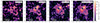 |
Fig. A.1. Mg II NB image of the nebula as constructed in Sect. 4.1 using the mosaic (10 h), udf-10 (31 h), MXDF (≈60 h) and a combination of the udf-10 and MXDF (≈90 h) MUSE data cubes. The legend is the same as in Fig. 3a. |
In the combined data, the shape of the Mg II nebula is reassuringly preserved, the S/N increased but the PSF is larger. For comparison we also show the appearance of the nebula in the ten-hour deep mosaic field, highlighting the fact that deep observations are crucial to study the CGM and IGrM of low-mass galaxies.
Appendix B: Smoothing effects on the detected nebula shape
Although our MUSE data are very deep (≈60 h, see Fig. 3b), the diffuse Mg II emission of the group revealed by such deep observations is still very faint. In order to increase the S/N, while keeping a spatial resolution that is as good as possible, we smoothed our data with a Gaussian kernel whose FWHM (3 MUSE pixels or  ) is slightly higher than the MUSE PSF FWHM (
 ).
).
Figure B.1 shows the dependence of the Mg II nebula S/N map on the smoothing kernel size. We choose to apply a smoothing as light as possible to keep an as good as possible spatial resolution.
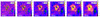 |
Fig. B.1. Mg II S/N map as constructed in Sect. 4.1 and smoothed using a 1, 2, 3, 4, 5, and 6 spaxel FWHM Gaussian from left to right, respectively. The FWHM values are indicated and shown as white circle (top right) in each panel. For comparison, the FWHM of the MUSE PSF is shown with a hatched white circle. The solid, dashed and dotted black contours correspond to a S/N of 1.5, 2 and 3, respectively. The adopted smoothing kernel has a FWHM of |

Appendix C: Spectral bandwidth effect on the Mg II nebula detection
As described in Sect. 4.1, the final Mg II NB image (Fig. 3a) has been optimized to encompass all the Mg II flux in the λ2796 and λ2803 lines while limiting the noise. The selected wavelength bands are shown by the shaded blue areas in the first panel of Fig. C.1 and indeed cover both the Mg II lines extracted in an area above the 2σ significance level (first panel). In order to emphasize the importance of optimizing the NB image and to check for any missing flux, we created a broader Mg II NB image (middle panel) encompassing the whole Mg II spectral range (2792−2806 Å in rest frame, purple shaded area in left panel). This broader-band (BB) Mg II image is noisier and the overall shape (green contour) of the nebula is lost in the noise. Looking at the residual image (i.e., the difference between the NB and BB Mg II images, right panel), we can see that, while some absorbing flux at the position of galaxy A is missed, all the emitting flux is captured by our NB construction procedure.
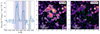 |
Fig. C.1. Spectral bandwidth effect on the Mg II nebula detection. Left: Mg II spectrum of the nebula integrated within the 2σ significance level contour (see Fig. 3a). The vertical blue shaded areas indicate the spectral widths used to construct the Mg II NB image shown in Fig. 3. The shaded purple area shows the wavelength band used to build the broader NB image shown in the middle panel. The hatched areas indicate the position of sky lines. Middle: Broader Mg II NB image extended by ±500 km s−1 on the λ2796 and λ2803 line outskirts (purple shaded area in the left panel) encompassing the whole Mg II spectral range (2792−2806 Å in rest frame). Right: Difference between the Mg II NB and broader band (blue and purple shaded areas in the left panel) images. The contours are the same as in Fig. 3 except that the green contour here shows the 1.5σ contour of the S/N-optimized Mg II NB image. |
Appendix D: Optically thin emission in the galaxy C line of sight
In Sect. 4.3 we rescaled the continuum radial SB profile to the Mg II radial SB value matching the position of galaxy C. This choice is motivated on the following basis:
-
the fact that the lines are well fitted by Gaussian functions (see Fig. D.1) indicates that the Mg II light emitted from galaxy C does not undergo strong radiative transfer (RT) effects or absorption.
-
the best-fit Mg II line flux ratio F2796/F2803 of 2.11±0.69 for galaxy C corresponds to optically thin emission and thus is in good agreement with a lack of RT effects and absorption in this line of sight.
-
as a resonant line, we can expect the so-called infilling effect to be significant for Mg II in this system. In other words, the absorbed photons can be re-emitted resonantly and escape the galaxy. As such, scattered Mg II photons can contribute to the spectrum of the galaxy by “filling” the Mg II absorption troughs. Mauerhofer et al. (2021) studied this effect for a simulated galaxy and found that it is more important for directions showing strong fluorescence lines. No fluorescent Fe II* lines are significantly detected in the galaxy C spectrum (Fig. 2, third line). The lack of infilling would reinforce the lack of scattering in the line of sight of galaxy C because the photons creating the infilling effect must have scattered at least once according to Mauerhofer et al. (2021).
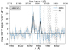 |
Fig. D.1. Mg II doublet line fitting of galaxy C. The best fit line (black) is shown along with the continuum subtracted ODHIN spectrum (blue). The uncertainties are shown in gray and the position of sky lines with gray hatches. |
To sum up, the lack of hints for absorption features and RT effects in the spectrum of galaxy C indicate that the Mg II emission is optically thin at the location of C. Those motivations justify our continuum rescaling procedure used to highlight the extended nature of the Mg II emission on radial SB profiles (Sect. 4.3).
Appendix E: Estimating the intrinsic Mg II photons budget using Cloudy modeling
E.1. Intrinsic nebular emission in H II regions
In order to predict an Mg II intrinsic stellar photon budget, we produced a grid of Cloudy models with a closed spherical geometry (Ferland et al. 2017). The input SEDs were created by combining the MAGPHYS intrinsic spectra for the group galaxies (obtained by fitting the Rafelski et al. 2015 HST photometry, see Sect. 3.2) with constant star-forming model SEDs obtained from the binary population synthesis code BPASSv2.2.1 (Eldridge et al. 2017) as shown in Fig. E.2. The BPASS SED was used to extend the MAGPHYS spectra to ionizing wavelengths. The age of the stellar population models was set to 108.75 years and the metallicity (Z) to two times solar, in accordance to the MAGPHYS best fit parameters. The stopping criteria of the calculations were set by the Hydrogen column density, with values between log10(NHstop) = 17 and 20 cm−2. This parameter cuts the calculation at some column density values inside the Stömgren Sphere. Finally, the luminosity of the models was set by the amount of hydrogen ionizing photons (log(q(H)) ≃ 51 photons s−1), constraining the ionization parameter to log⟨U⟩≃ − 2.6.
We adopt two different prescriptions for the element abundances in the cloud: (1) solar abundance ratios from Grevesse et al. (2010) where  and, (2) ISM abundances based on the mean warm and cold phases of the ISM (
 ). It is noteworthy to mention that (1) does not include grains, while (2) has a combination of silicates and graphites defined by Mathis et al. (1977). The results of these models can be seen in Figure E.1, in which we show how the intrinsic Mg II to [O II] ratio changes as a function of the stopping column density. We find that the models provide a higher intrinsic Mg II to [O II] ratio than the observed one (where dust attenuation and scattering might explain the discrepancy) when considering solar abundance ratios and ISM abundances with a stopping column density > 1018 cm−2. This suggests that the Mg II emission of the nebula can be explained by stellar processes alone through resonant scattering of photons originally produced in H II regions.
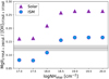 |
Fig. E.1. Predicted intrinsic nebular Mg II to [O II] ratio using Cloudy models constrained by the best fit parameters of the observations (see SEDs in the right panel). The symbols represent the chemical abundances used, triangles for solar and circles for ISM. The horizontal gray line and shaded area show the observed Mg II to [O II] ratio from the group and the 1σ uncertainties, respectively. |
E.2. Comparison between the stellar versus UVB contribution to the Mg II nebulae
In order to assess the origin of the Mg+ ionizing photons (λ < 825 Å), leading to the emission of Mg II photons, we compare the total SED of the group members (sum of the five SEDs, see Sect. E.1) with the UVB SED from Haardt & Madau (2012) at the redshift of the group (i.e., z = 1.3). Those SEDs are in rest frame and show the flux as it would be observed at a distance varying between 10 and 35 kpc of the stars. This range in radius allowed us to evaluate and compare the contributions of the stars and UVB at the edge of the detected nebula as well as closer to the galaxies. We show two models with arbitrary values of the escape fractions 0.7% and 14% (log10(NHstop) = 18 and 18.5, respectively), calculated as the transmitted to intrinsic ratio of the flux integrated < 912 Å.
In Figure E.2 we show that the contribution of the UVB to the Mg+ ionizing flux (λ < 825 Å or E > 15.04 eV) is dominant in the nebula (10 < r [kpc] < 35) only when considering an ionizing escape fraction close to zero. When getting closer to the stars (r < 10 kpc), the contribution of the UV stellar emission becomes dominant. At higher escape fractions (e.g., 14% as shown on the figure), the contribution of the UVB quickly becomes negligible, even at the outskirts of the nebula.
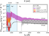 |
Fig. E.2. Comparison of the UVB vs stellar photons budget, ionizing Mg+ in Mg2+. In purple we show the intrinsic BPASS model for Z = 2 Z⊙ and age of 108.75 years for a constant SF stellar population. The transmitted BPASS model considering 0.7% and 14% ionizing escape fraction is shown in red and orange, respectively. The gray spectrum shows the attenuated spectrum of the group (sum of five SEDs, Sect. E.1). The dispersion of all spectra depends on the radius at which we estimate the flux, the lower and upper boundaries of the areas are for 35 and 10 kpc, respectively. The black dashed line shows the UVB from Haardt & Madau (2012) at z = 1.3. |
All Tables
All Figures
|
Fig. 1. Galaxy group and its environment. Left: galaxies belonging to the same structure (see Sect. 3.1) as the galaxies embedded in the z ≈ 1.31 Mg II nebula (shown as the red square) are indicated by white squares. The velocity relative to the most massive galaxy of the group (galaxy A, see middle panel) is indicated for each galaxy in km s−1. The structure spans ≈2 Mpc in projection and the galaxies appear well aligned. A ≈1 Mpc substructure extending beyond the MUSE Deep Field (big black dashed square) is also indicated. The MXDF and udf-10 fields are shown with the solid circle and small dashed square, respectively. The background image is an MPG(ESO2.2m)/WFI image (Hildebrandt et al. 2006). Middle: zoom-in window of (12 |
| In the text | |
|
Fig. 2. Integrated spectra of the five group members. Left: 2″ × 2″ HST/ACS F775W images of the five group members. The central white cross and contour indicate the HST coordinates and segmentation map from Rafelski et al. (2015). Right: integrated spectrum (units of 10−20 erg s−1 cm−2 Å−1) of the galaxy shown in the corresponding left panel extracted within the HST segmentation map contour using the ODHIN software (Bacher 2017, see Sect. 3.3) and smoothed with a 7 Å FWHM Gaussian function. The positions of several emission (absorption) lines are indicated by vertical dotted green (red) lines. The gray unsmoothed spectra show the 1σ uncertainties which have been offset for readability. The unsmoothed Mg II and [O II] lines (vertical dashed lines) are shown in the insets. The vertical blue shaded areas indicate the spectral widths used to construct the Mg II NB image shown in Fig. 3a. |
| In the text | |
|
Fig. 3. Metal-enriched intragroup medium revealed by MUSE. (a) Mg II narrow-band image of the group (see Sect. 4.1) smoothed with a 0.6″ FWHM Gaussian and plotted with a power-law stretch. The white contours correspond to Mg II significance levels of 1.5, 2 and 3σ (solid, dashed, and dotted, respectively) where 1σ corresponds to a SB level of 1 × 10⁻¹⁹ erg s−1 cm−2 arcsec−2. The blue contours indicate the negative SB values (same coding as the positive contours) corresponding to the absorbing regions (see Sect. 4.2). The green contours trace the continuum of the group members close to Mg II and the neighboring galaxies as detected in the HST/ACS F775W image. The dotted green contour corresponds to the outer HST continuum contours of the group members set at the MUSE resolution. The FWHM of the MUSE PSF and smoothing kernel are shown with a hatched and empty circle, respectively, at the bottom-right of the figure. (b) Exposure map centered on the group. The solid, dashed, and dotted black contours indicate 10, 30, and 90 h depth, respectively. The white contour corresponds to the Mg II significance level of 1.5σ. (c) Mg II absorption in the spectrum of the background galaxy BKG located at an impact parameter of 19 kpc from galaxy D in projection and at the nebula redshift. The blue line is the best-fit model of the Mg II doublet absorption (Sect. 4.2). The 1σ uncertainties are shown in gray and the hatched areas indicate the position of strong sky lines and noise peaks. The systemic redshift of galaxy D is indicated by vertical dashed lines. |
| In the text | |
|
Fig. 4. Channel maps around the Mg IIλ2796 emission. Each map corresponds to one MUSE subcube slice (1.25 Å or 58 km s−1 at the redshift of the group). The velocity window relative to the systemic redshift of galaxy A is indicated on each panel. Contours are the same as in Fig. 3a. The eight central slices (from −177 to +286 km s−1) are summed to create the optimized λ2796 Mg II NB image shown in Fig. 3a (see Sect. 4.1). |
| In the text | |
|
Fig. 5. Azimuthally averaged radial surface brightness profile of the Mg II nebula centered on galaxy A (blue data points). For comparison the profile of the Mg II continuum (±20 000 km s−1 around the Mg II doublet) shown in black is also rescaled (gray) to the Mg II SB at the location of galaxy C (where Mg II absorption is unlikely, see Appendix D). The positions of the group members are indicated with vertical dashed lines. The radial profiles have been calculated using unsmoothed Mg II and continuum images after masking the pixels outside the 1σ significance level approximated with an elliptical contour as shown in the inset (left). Middle and right panels: radial profiles after masking the pixels above and below the [A,B,C] axis, respectively. In the insets, we also show the two-pixel annuli used to construct the profiles as white circles. |
| In the text | |
|
Fig. 6. Spatially resolved Mg II and [O II] properties. Left: binned line-of-sight velocity maps of the Mg II (top) and [O II] (bottom) emission relative to the systemic redshift of galaxy A (Sects. 4.4 and 5.1). The black contours correspond to the 1.5σ significance level. The green contours trace the galaxies detected in the HST/ACS F775W image. The FWHM of the MUSE PSF and smoothing kernel are shown with a hatched and an empty circle, respectively, at the top right of the panels. The diverging Mg II and [O II] colormaps are centered on the systemic redshift of galaxy A and have the same dynamical range to ease the visual comparison (Sect. 5.1). Right: Mg II (top) and [O II] (bottom panels) doublet extracted in the elliptical areas traced in purple and designated by the same number on the map (left panels). The vertical dashed lines correspond to the systemic redshift of galaxy A. The vertical hatched bands indicate the presence of sky lines. |
| In the text | |
|
Fig. 7. [O II] and Fe II* spatial properties. First column: [O II] NB image (top, Sect. 5.1). Legend is the same as in Fig. 3a. The 1σ level corresponds to a SB of 2.5 × 10⁻¹⁹ erg s−1 cm−2 arcsec−2. Bottom panels: total and directional (below and above the [A,B,C] axis) azimuthally averaged radial SB profiles centered on galaxy A (from top to bottom, respectively, see also insets for illustration) of the [O II], [O II] continuum and rescaled [O II] continuum (orange, black and gray, respectively) emission. The radial positions of other group members with respect to galaxy A are indicated by the vertical dashed lines. Second column: same as first column but for Fe II* (purple). Third column: comparison of the Mg II, [O II] and Fe II* 2σ significance level contours (blue, orange, and purple, respectively) superimposed on the Mg II NB image (top). Bottom panels: show a comparison of the radial SB profiles where the Fe II* profile (shaded purple) has been rescaled to the [O II] profile at the SB peak and Mg II (shaded blue) at the position of galaxy C (Appendix D). For this plot the [O II] map was degraded to the resolution of the Mg II emission (Sect. 5.1). |
| In the text | |
|
Fig. A.1. Mg II NB image of the nebula as constructed in Sect. 4.1 using the mosaic (10 h), udf-10 (31 h), MXDF (≈60 h) and a combination of the udf-10 and MXDF (≈90 h) MUSE data cubes. The legend is the same as in Fig. 3a. |
| In the text | |
|
Fig. B.1. Mg II S/N map as constructed in Sect. 4.1 and smoothed using a 1, 2, 3, 4, 5, and 6 spaxel FWHM Gaussian from left to right, respectively. The FWHM values are indicated and shown as white circle (top right) in each panel. For comparison, the FWHM of the MUSE PSF is shown with a hatched white circle. The solid, dashed and dotted black contours correspond to a S/N of 1.5, 2 and 3, respectively. The adopted smoothing kernel has a FWHM of |
| In the text | |
|
Fig. C.1. Spectral bandwidth effect on the Mg II nebula detection. Left: Mg II spectrum of the nebula integrated within the 2σ significance level contour (see Fig. 3a). The vertical blue shaded areas indicate the spectral widths used to construct the Mg II NB image shown in Fig. 3. The shaded purple area shows the wavelength band used to build the broader NB image shown in the middle panel. The hatched areas indicate the position of sky lines. Middle: Broader Mg II NB image extended by ±500 km s−1 on the λ2796 and λ2803 line outskirts (purple shaded area in the left panel) encompassing the whole Mg II spectral range (2792−2806 Å in rest frame). Right: Difference between the Mg II NB and broader band (blue and purple shaded areas in the left panel) images. The contours are the same as in Fig. 3 except that the green contour here shows the 1.5σ contour of the S/N-optimized Mg II NB image. |
| In the text | |
|
Fig. D.1. Mg II doublet line fitting of galaxy C. The best fit line (black) is shown along with the continuum subtracted ODHIN spectrum (blue). The uncertainties are shown in gray and the position of sky lines with gray hatches. |
| In the text | |
|
Fig. E.1. Predicted intrinsic nebular Mg II to [O II] ratio using Cloudy models constrained by the best fit parameters of the observations (see SEDs in the right panel). The symbols represent the chemical abundances used, triangles for solar and circles for ISM. The horizontal gray line and shaded area show the observed Mg II to [O II] ratio from the group and the 1σ uncertainties, respectively. |
| In the text | |
|
Fig. E.2. Comparison of the UVB vs stellar photons budget, ionizing Mg+ in Mg2+. In purple we show the intrinsic BPASS model for Z = 2 Z⊙ and age of 108.75 years for a constant SF stellar population. The transmitted BPASS model considering 0.7% and 14% ionizing escape fraction is shown in red and orange, respectively. The gray spectrum shows the attenuated spectrum of the group (sum of five SEDs, Sect. E.1). The dispersion of all spectra depends on the radius at which we estimate the flux, the lower and upper boundaries of the areas are for 35 and 10 kpc, respectively. The black dashed line shows the UVB from Haardt & Madau (2012) at z = 1.3. |
| In the text | |
Current usage metrics show cumulative count of Article Views (full-text article views including HTML views, PDF and ePub downloads, according to the available data) and Abstracts Views on Vision4Press platform.
Data correspond to usage on the plateform after 2015. The current usage metrics is available 48-96 hours after online publication and is updated daily on week days.
Initial download of the metrics may take a while.