| Issue |
A&A
Volume 691, November 2024
|
|
|---|---|---|
| Article Number | A222 | |
| Number of page(s) | 9 | |
| Section | Extragalactic astronomy | |
| DOI | https://doi.org/10.1051/0004-6361/202450609 | |
| Published online | 15 November 2024 | |
The stellar population of a z ∼ 3.25 Lyα-emitting group associated with a damped Lyα absorber
1
Dipartimento di Fisica G. Occhialini, Università degli Studi di Milano Bicocca, Piazza della Scienza 3, 20126 Milano, Italy
2
Institute for Astronomy, University of Edinburgh, Blackford Hill, Edinburgh EH9 3HJ, UK
3
INAF – Osservatorio Astronomico di Trieste, Via G. B. Tiepolo 11, I-34143 Trieste, Italy
4
Space Telescope Science Institute, 3700 San Martin Drive, Baltimore, MD 21218, USA
5
Department of Physics and Astronomy, Johns Hopkins University, Baltimore, MD 21218, USA
6
Department of Physics, ETH Zürich, Wolfgang-Pauli-Strasse 27, Zürich 8093, Switzerland
7
Institute for Computational Cosmology, Department of Physics, Durham University, South Road, Durham DH1 3LE, UK
⋆ Corresponding authors; This email address is being protected from spambots. You need JavaScript enabled to view it.
, This email address is being protected from spambots. You need JavaScript enabled to view it.
Received:
3
May
2024
Accepted:
16
September
2024
Abstract
We present near-infrared observations, acquired with the Wide Field Camera 3 (WFC3) on board the Hubble Space Telescope (HST), of a Lyα-emitting double-clumped nebula at z ≈ 3.25 associated with a damped Lyα absorber (DLA). With the WFC3/F160W data we observe the stellar continuum around 3600 Å in the rest frame of a galaxy embedded in the west clump of the nebula, GW, for which we estimate a star formation rate (SFR) of SFRGW = 5.0 ± 0.4 M⊙ yr−1 and a maximum stellar mass MGW < 9.9 ± 0.7 × 10⁹ M⊙. With the enhanced spatial resolution of HST, we discover the presence of an additional faint source, GE, in the center of the east clump, with SFRGE = 0.70 ± 0.20 M⊙ yr−1 and a maximum stellar mass MGE < 1.4 ± 0.4 × 10⁹ M⊙. We show that the Lyα emission in the two clumps can be explained by recombination following in situ photoionization by the two galaxies, assuming escape fractions of ionizing photons of ≲0.24 for GW and ≲0.34 for GE. The fact that GW is offset by ≈8 kpc from the west clump means we cannot fully rule out the presence of additional fainter star-forming sources, which would further contribute to the photon budget inside this ≈1012 M⊙ galaxy group that extends over a region of 30 × 50 kpc.
Key words: galaxies: groups: general / galaxies: halos / galaxies: high-redshift / quasars: absorption lines
© The Authors 2024
 Open Access article, published by EDP Sciences, under the terms of the Creative Commons Attribution License (https://creativecommons.org/licenses/by/4.0), which permits unrestricted use, distribution, and reproduction in any medium, provided the original work is properly cited.
This article is published in open access under the Subscribe to Open model. This email address is being protected from spambots. You need JavaScript enabled to view it. to support open access publication.
1. Introduction
Spectroscopy with large-format integral field units (IFUs) on 8m class telescopes has rapidly transformed our view of the circumgalactic medium (CGM), the heterogeneous diffuse gas around galaxies that plays a key role in the regulation of the baryon cycle. Once the realm of absorption spectroscopy alone, the study of the CGM has rapidly progressed thanks to the Multi Unit Spectroscopic Explorer (MUSE; Bacon et al. 2010) at the Very Large Telescope (VLT) and other IFUs such as the Keck Cosmic Web Imager (KCWI; Morrissey et al. 2018). With these instruments, halo gas is routinely mapped in Lyα emission on scales of up to ≈100 kpc near star-forming galaxies (Wisotzki et al. 2016; Leclercq et al. 2017) and quasars (Borisova et al. 2016; Arrigoni et al. 2019; Fossati et al. 2021), metals in emission have been imaged in the inner CGM of both active galactic nuclei and star-forming systems (Guo et al. 2020, 2023; Fossati et al. 2021; Dutta et al. 2023), and cosmic web filaments connecting multiple galaxies have been unveiled in low-surface-brightness Lyα maps (Umehata et al. 2019; Bacon et al. 2021).
Unlike traditional techniques such as multi-object spectroscopy employed, for example, in the Keck Baryonic Structure Survey (KBSS; Rudie et al. 2012; Steidel et al. 2014) and in the VLT Lyman break galaxy Redshift Survey (VLRS; e.g., Shanks et al. 2011; Bielby et al. 2011; Crighton et al. 2011), IFUs do not require any preselection of galaxies. This advantage has made IFUs a common tool for studying galaxies associated with absorption line systems, and many sources at smaller impact parameters that went undetected when observed with other instruments have been revealed. Furthermore, thanks to dedicated surveys targeting continuum faint Lyα or [OII] emitters (e.g., Schroetter et al. 2016; Péroux et al. 2019; Lofthouse et al. 2020; Muzahid et al. 2020; Oyarzún et al. 2024), samples of absorbers and galaxy associations have increased in size from a few tens to several thousand. At z ≈ 0.5 − 1.5, the MUSE Analysis of Gas around Galaxies (MAGG) survey (Dutta et al. 2020) has expanded the results of multi-object spectrographs (Chen et al. 2018; Weiner et al. 2009) to higher redshifts (z ≈ 1.5), revealing that stellar mass is the dominant factor influencing the Mg II absorption around galaxies. By focusing on the inner CGM traced by very strong Mg II absorption systems, the MUSE Gas Flow and Wind (MEGAFLOW) survey (Schroetter et al. 2016) has provided an expanded view of the effects of inflows and outflows on the column density and kinematic distributions of the absorbing gas around the host galaxy as a function of the galaxy orientation. At higher redshifts, z ≳ 3, the MUSE Quasar Field Blind Emitter Survey (MUSEQuBES; Muzahid et al. 2020) and the MAGG survey (Lofthouse et al. 2020, 2023; Galbiati et al. 2023) have extended our view of the properties of hydrogen and metals (traced by C IV and Si IV) around continuum-faint Lyα emitters (LAEs), reaching ≈1 dex lower masses compared to previous studies that used brighter Lyman break galaxies (LBGs). These studies have revealed the presence of gas filaments that host strong hydrogen and metal absorbers and stretch across galaxies, as well as diffuse pockets of lower column densities and enriched gas.
The analysis of the galactic environment around metal absorbers has been pushed to even higher redshifts (z ≳ 4) thanks to the combined power of the Near Infrared Camera (NIRCam) slitless grism spectrograph on board the James Webb Space Telescope (JWST) and the Atacama Large Millimeter Array (ALMA). These studies revealed the presence of galaxies at impact parameters < 300 kpc from low-ionization metal absorbers, suggesting the presence of an efficient intergalactic medium enrichment mechanism during the later stages of reionization (e.g., Wu et al. 2023; Bordoloi et al. 2024).
Thanks to integral field spectroscopy, it has become clear that absorption line systems are often associated with multiple galaxies, including cases of rich galaxy groups with up to ≈10 members. These rich groups present more extended distributions of both hydrogen and metal-enriched gas (Bordoloi et al. 2011; Fossati et al. 2021; Dutta et al. 2020; Galbiati et al. 2023; Lofthouse et al. 2023; Muzahid et al. 2021), with covering factors ≈2 − 5 times higher than those of isolated galaxies. While the mechanisms responsible for this elevated gas distribution remain unconstrained, studies of individual cases in which tomography in absorption is possible or enriched gas in emission can be probed (Fossati et al. 2019; Chen et al. 2019; Leclercq et al. 2022) point to gravitational interactions and outflows as possible mechanisms that can increase the contribution arising from the superposition of halos or a more diffuse intragroup medium.
Among the first examples of absorption line systems associated with group environments observed by MUSE, Fumagalli et al. (2017) reported the detection of a damped Lyα absorber (DLA) with a column density of log NHI = 20.85 ± 0.10 cm−2 at redshift zdla = 3.2552 ± 0.0001. This DLA is associated with a UV-continuum-detected galaxy at a projected distance of 19.1 ± 0.05 kpc, embedded in an extended Lyα nebula composed of two bright clumps separated by a projected distance of 16.5 ± 0.5 kpc. The line-of-sight velocity of the two emitting Lyα clumps is aligned in velocity with the main absorption components of metal lines associated with the DLA, which suggests a link between the absorption and emission substructures. This evidence is consistent with multiple galaxies forming inside an extended gas-rich and metal-rich structure. As the two clumps were detected only via Lyα, uncertainty remained about the nature of this emitting region and the possible powering mechanisms.
To address these questions, we collected near-infrared (NIR) imaging (PID 15283; PI: Mackenzie) using the F160W filter with Wide Field Camera 3 (WFC3) on board the Hubble Space Telescope (HST) to search for rest-frame optical emission and better constrain the properties of this system through stellar population synthesis analysis. This paper discusses the HST NIR follow-up observations and expands on the conclusions presented in Fumagalli et al. (2017). The structure of the paper is as follows. In Sect. 2 we present the new observations and data reduction, followed by the analysis in Sect. 3 and a discussion on the nature of the Lyα emission origin and the associated galaxy environment in Sect. 4. The summary and conclusions are presented in Sect. 5. Unless otherwise noted, we quote magnitudes in the AB system, distances in proper units, and adopt the Planck 2015 cosmology (Ωm = 0.307, H0 = 67.7 km s−1 Mpc−1; Planck Collaboration XIII 2016).
2. MUSE and HST observations
2.1. Spectroscopy from MUSE
The quasar J0255+0048 was first observed thanks to an imaging survey aiming to probe in situ star formation associated with DLAs (O’Meara et al. 2006; Fumagalli et al. 2010). From this survey, J0255+0048 and other five quasars were selected as systems hosting DLAs at z > 3, the redshift for which Lyα enters the wavelength range covered by MUSE, allowing the gathering of additional data. MUSE observations of these six quasar fields were conducted at the VLT as part of the European Southern Observatory (ESO) programs 095.A-0051 and 096.A-0022 (PI: Fumagalli). Observations were carried out on the nights of 17−20 September 2015 in a series of 1500 s exposures, with a total of 2.5 hours under good seeing conditions (requested to be  ) and clear sky.
The detailed data reduction process is presented in Fumagalli et al. (2017); only the key steps are highlighted here. Following the standard ESO MUSE pipeline (v1.6.2; Weilbacher et al. 2014), basic corrections such as bias subtraction and flat-fielding were applied in addition to wavelength and photometry calibrations. The frames were then processed to improve the quality of sky subtraction and flat-fielding and to remove the residuals left from the ESO pipeline reduction using the CUBEXTRACTOR code (CUBEX; Cantalupo et al. 2019). Corrections for extinction were implemented. From comparisons with photometric data from the Sloan Digital Sky Survey (Eisenstein et al. 2011) a factor of 1.12 was applied to the flux calibration to consider low levels of atmospheric extinction. Following Schlafly & Finkbeiner (2011), the presence of Milky Way dust in the direction of observation was evaluated. The final IFU cube has a field of view of 1 × 1 arcmin2 composed by 0 2 pixels, covering the wavelength range 4750−9350 Å in bins of 1.25 Å. At λ ≈ 5170 Å, corresponding to the Lyα wavelength at the DLA redshift, the effective image quality is
  and the noise level ≈6 × 10⁻¹⁹ erg s−1 cm−2 Å−1 arcsec−2 (root mean square).
2.2. Near-infrared imaging from HST
The field of quasar J0255+0048 was imaged over four orbits with HST WFC3/IR F160W (PID 15283; PI: Mackenzie). Observations were obtained on 28 August 2018 and 15 September 2019. The bright quasar has H(AB) = 18.33 mag, several magnitudes brighter than the targeted nebula counterparts at a separation of 2 − 6″. Given this magnitude contrast, ensuring that the quasar did not contaminate the structure either through diffraction spikes or by dithering the structure onto pixels affected by persistence from the bright quasar was critical. To minimize the impact of diffraction spikes, we selected only ORIENT angles that place the diffraction spikes away from the structure identified in Lyα emission.
There is a bright star with H(AB)≈9.0 mag ≈45″ away from the quasar and the Lyα nebula. The star is sufficiently bright that it would quickly saturate the detector and its extended point spread function (PSF) would contaminate the object of interest. We therefore offset the exposures from the default aperture so that the star falls outside the field of view to the greatest extent possible. This resulted in our target being placed in one corner of the observed field, with diffraction spikes from the star that do not overlap with our target source.
To control persistence and dither to improve spatial sampling, we adopted the LINE dither pattern with 1.5″ point spacing to move along the line separating the quasar and the Lyα nebula. In this way, the structure never fell on pixels that the quasar had fallen on in previous exposures. The larger point spacing (≈3×) allows the removal of IR blobs and other artifacts for cleaner images. To maximize the signal-to-noise ratio for any faint counterparts of the Lyα nebula, we used SPARS50 with NSAMP = 14, resulting in four exposures per orbit over three orbits.
The observations in 2019 were repeated because observations from 2018 failed due to a guide star reacquisition failure, resulting in the loss of an exposure. The orientation constraints required to avoid the diffraction spikes delayed the repeat for a year. This provided an opportunity to further avoid the diffraction spikes of the bright nearby star for a more fully cleaned image. Thus, we slightly offset the target location of this repeated visit. We obtained an additional four exposures over one orbit with the same dither pattern and sampling as the original data, although at a different orientation (U3 = 272.2° compared to U3 = 274.0° for the original visit). In total, we obtained 9794 s of successful exposure time over 15 dithered exposures.
The data were downloaded from the Mikulski Archive for Space Telescope (MAST) in 2022 to obtain data calibrated with the IR filter-dependent delta sky flats by date of appearance of IR blobs (WFC3 ISR 2021–01; Olszewski & Mack 2021). Custom masks were created to remove the diffraction spikes from the nearby star and satellite trails. The individual exposures were first aligned to each other with TWEAKREG. Then the resultant combined image mosaic generated with ASTRODRIZZLE was aligned using Gaia Early Data Release 3 (Gaia Collaboration 2021) with uncertainties  . The following drizzle parameters were used: COMBINE_TYPE was set to “imedian”, SKYMETHOD to “globalmin+match”, FINAL_WHT_TYPE to “IVM”, FINAL_SCALE to 0.06, FINAL_PIXFRAC to 0.8, and FINAL_ROT to 0.
Root mean square (RMS) error images were created from the resultant weight (WHT) map, where  . We corrected the RMS maps for correlated pixel noise as described in Sect. 3.3.2 of the DRIZZLEPAC Handbook (v2.0, Hoffmann et al. 2021), which provides a noise scaling factor (R) based on the drizzled and native pixel scales, and the FINAL_PIXFRAC. For our drizzle parameters, the noise scaling factor is R = 1.71, yielding a correlated noise factor of 2.124.
3. Analysis of HST imaging data
With HST NIR follow-up observations, we find two sources, labeled GE and GW, detected in emission in the region of the double-clumped Lyα nebula. Here, GW is the galaxy previously named G in Fumagalli et al. (2017). The two sources are separated by a projected distance of  , ≈23 kpc at the DLA redshift zdla, with a projected distance between GE and the quasar of ≈40 kpc and between GW and the quasar of ≈19.5 kpc.
From the comparison between the Lyα emission and the HST NIR observations in Fig. 1, we find that a third (≈33% in the case of GW and ≈27% for GE) of the total Lyα emission of the nebula is detected inside the 1″ circular apertures around the two sources (solid purple circles), suggesting a connection between the star formation activity within the detected galaxies and the Lyα emission. Moreover, when comparing the centers of the two Lyα-emitting clumps, CW and CE, with the centers of the two galaxies detected in the continuum, we find an offset of ≈7.7 kpc between GW and CW and ≈1.6 kpc between GE and CE. GW has a spectrum and colors consistent with those of a z ≈ 3.2 LBG (Fumagalli et al. 2017). We do not have previous information about the second galaxy, GE, because its fainter continuum emission is not detected by MUSE. However, the fact that GE is well centered in correspondence of the Lyα-emitting clump CE is indicative of a true association rather than a spurious projection effect. For this reason, the redshift of both galaxies is assumed to be that of the DLA, zdla = 3.2552 ± 0.0001. At the estimated redshift of these galaxies, the [O III] and Hα lines could be observed at wavelengths much higher than the ones covered by the F160W filter. Other lines that can fall in the observed wavelength range generally have lower equivalent widths, and for this reason, no contribution from emission lines is included.
3.1. Photometry
Flux from the bright quasar J0255+0048 needs to be subtracted to accurately compute the flux emitted by the two sources. The quasar contribution within the circular aperture of 1″ around GE is consistent with zero within the background uncertainty and, therefore, negligible. For GW, a subtraction of the quasar PSF with a bespoke code developed for HST/WFC3 PSF modeling (Revalski 2022; Revalski et al. 2023) suppressed the quasar contamination in the circular area of 1″ radius around GW to levels comparable with zero given the background uncertainty. All the background uncertainties related to a given aperture in the science image are evaluated as the square root of the quadrature sum of the values displayed by the pixels of the RMS image inside the same aperture.
To measure the flux emitted by GW, we used the SOURCE EXTRACTOR Python library (Bertin & Arnouts 1996; Barbary 2018) and computed the signal contained inside the Kron elliptical aperture associated with the galaxy, expected to encircle 94% of the total flux (Kron 1980; Bertin & Arnouts 1996). The measured value was then divided by a factor of 0.94 to derive the total flux. Figure 2a shows in purple the measured Kron flux for GW,  erg s−1 cm−2 Å−1. The corresponding AB magnitude is m(AB)GW = 24.71 ± 0.08 mag. Uncertainties on flux measured inside a given aperture were evaluated as the square root of the quadrature sum of the Poisson uncertainty related to the measured flux and the background uncertainty from the RMS image derived above. The Kron flux is consistent with the flux estimated from the growth curve,
  erg s−1 cm−2 Å−1, indicated in yellow in Fig. 2a.
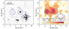 |
Fig. 1. HST data of the two continuum-emitting sources GE and GW inside the Lyα-emitting nebula observed with MUSE. Left: HST WFC3/F160W observation with the subtracted quasar PSF. The two sources GE and GW are indicated by the purple circular apertures of |


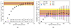 |
Fig. 2. Growth curve for galaxies GW (a) and GE (b). The black points show the resulting flux with background and shot-noise uncertainties. The Kron flux is represented in purple with the shaded 68% confidence region. The growth curve flux is marked in yellow with the shaded 68% confidence region. In panel b, the colored squares represent the flux observed inside the apertures that encircle 70.8%, 83.6%, 86.3%, and 90.0% of the total energy emitted by a point-like source. |
We repeated the analysis for GE, using both the Kron flux and the growth curve method. The purple line in Fig. 2b marks the total flux evaluated from the elliptical Kron aperture ( erg s−1 cm−2 Å−1). The source GE is much fainter and compact, and the resulting growth curve is noisier. For estimating the total flux, we therefore applied an aperture correction, relying on the values published in the WFC3/IR handbook. The flux values in the apertures encircling 70.8%, 83.6%, 86.3%, and 90% of the total energy are shown as colored squares in Fig. 2b. At radii
  the noise becomes considerable. We hence relied on the aperture at
  (blue square), obtaining a total aperture-corrected flux fGE = 8.3 ± 2.4 × 10⁻²¹ erg s−1 cm−2 Å−1.
The Kron and growth curve fluxes are consistent with each other at 1σ level, as the substantial uncertainties easily accommodate the ≈10% difference. In the following, we adopt as the best estimate the value of the flux obtained from the growth curve. The apparent magnitude of GE thus becomes m(AB)GE = 26.9 ± 0.2 mag. Information relative to the two sources is summarized in Table 1.
Properties of galaxies GW and GE.
3.2. Star formation rate and stellar mass evaluation
To evaluate the stellar mass of the two sources, we simulated the spectral evolution using the STARBURST99 software (Leitherer et al. 1999), assuming Geneva stellar tracks without rotation and a metallicity comparable to that of the DLA, Z = 0.002 (Z ≃ 0.1 Z⊙). We assumed a Kroupa (Kroupa 2001) initial mass function, represented by a double power law with index α1 = 1.3 between 0.1 and 0.5 M⊙ and α2 = 2.3 between 0.5 and 100 M⊙. Dust is not considered by STARBURST99 models; however, even if dust is not expected to significantly affect LAEs, we discuss the consequences of the presence of dust at the end of this section. Due to the limited number of photometric data points available, we are unable to accurately constrain all the necessary properties, such as dust content, age, and star formation history, required to estimate the stellar mass of the galaxies. As a result, we had to proceed with our analysis by introducing assumptions, some of which are testable, with the aim of establishing an upper limit for the stellar mass of the two sources.
To explore the properties of GW we considered the evolution of a galaxy with a constant star formation rate (SFR) ranging from 0.1 to 10 M⊙ yr−1, evaluating the flux that would produce in the F160W filter if it were observed at the DLA redshift zdla = 3.2552. The results are shown in Fig. 3a, in which the color illustrates the value of the synthetic IR flux as a function of SFR and age. The black solid and dash-dotted lines enclose the 68% and 95% confidence intervals around the measured value of  . We observe that the SFR implied by the F160W magnitude strongly depends on age for ages < 2 Gyr, but it is relatively constant thereafter. This trend arises from the fact that the F160W band has a pivot wavelength at λF160W = 15 369 Å, corresponding to a rest frame emission of λrf ≃ 3612 Å, which is at the boundary between the near-UV (NUV) and optical bands. The NUV part of the spectrum is more sensitive to the SFR of the galaxy, but the probed wavelengths are red enough to be also affected by the growth of the stellar mass. Due to the additional contribution from older stellar populations at a later time, the same flux can be obtained with a lower SFR than at earlier times. To find an upper limit for the mass of the galaxy, we formulated the hypothesis that the age of the galaxy is approximately equal to the age of the Universe at the observed redshift (i.e., t ≃ 1.97 Gyr, marked by the white vertical line in Fig. 3a), deriving an average SFRGW = 5.0 ± 0.4 M⊙ yr−1.
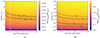 |
Fig. 3. F160W simulated flux at z = 3.25 as a function of SFR and age, assuming a constant SFR evolution. The solid and dash-dotted black lines are the 1σ and 2σ confidence intervals of the measured flux of galaxy GW (a) and GE (b). The white line marks the age of the Universe at z = 3.25 (i.e., t = 1.97 Gyr); based on this age, the average SFR of the two sources is inferred to be SFRGW = 5.0 ± 0.4 M⊙ yr−1 and SFRGE = 0.70 ± 0.20 M⊙ yr−1. |
The assumption of constant star formation history for galaxy GW can be tested using the observed r-band flux of fr = 16 ± 1 × 10⁻²⁰ erg cm−2 s−1 Å−1 computed by Fumagalli et al. (2017) through the convolution of MUSE spectroscopic data with the r filter response. The observed r-band flux, with a pivot wavelength λr ≈ 6176 Å, is more sensitive to the instantaneous SFR of the galaxy as it is probing the rest frame far-UV (FUV) flux with λr, rf ≈ 1451 Å. As before, we evaluated the synthetic r-band flux that galaxies with different values of SFR should emit and compare them with what observed for galaxy GW. The results showed in Fig. 4 demonstrate how the r-band flux can be considered independent of the age of the galaxy under the assumption of constant star formation history and the instantaneous SFR of galaxy GW is measured to be SFRGW = 4.6 ± 0.3 M⊙ yr−1. In Fig. 5, we compare the more instantaneous SFR value inferred from the r-band flux (green line) with the indicator on longer timescales from the F160W photometry (orange line). The shaded regions mark the 1σ and 2σ confidence intervals on the measured fluxes. The fact that at t ≃ 1.97 Gyr, the assumed age of GW, the instantaneous SFR is comparable with the averaged SFR obtained from F160W observations rules out significant excursions in the recent star formation history of the galaxy. The slightly lower value of the inferred instantaneous SFR could be explained by a past enhancement in the star formation activity of GW. Still, the difference is within current uncertainties.
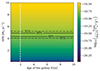 |
Fig. 4. Simulated r-band flux as a function of the galaxy age and SFR, assuming a constant star formation history. The solid and dashed black lines are the 1σ and 2σ confidence intervals of the r flux estimation measured with MUSE data by Fumagalli et al. (2017). The dashed white line marks the age of the Universe at z = 3.25, i.e., t = 1.97 Gyr. The r-band flux is more sensitive to the instantaneous SFR and, under the assumption of a constant star formation history used in this case, does not depend on the age of the galaxy. |
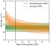 |
Fig. 5. Comparison between the inferred instantaneous SFR (green) inferred from the r-band flux and the value averaged over longer timescales (orange) from the F160W photometry of galaxy GW. The dark- and light-shaded regions mark the 68% and 95% confidence intervals. The similarity between the two values corroborates the hypothesis of a constant SFR. |
The straw-man assumption of t ≃ 1.97 Gyr can be compared to what is found in the stellar populations of LAEs. For example, recent studies suggest that LAEs have typical ages of ≲500 Myr (e.g., Matthee et al. 2021; Endsley et al. 2024). If that were the case, we would derive an average SFR for GW of ≳6.1 M⊙ yr−1, a factor of 1.3 higher than the instantaneous SFR, suggesting that the galaxy may have undergone a more significant starburst phase. Assuming a maximal age also provides an estimate for the galaxy maximum stellar mass using the relation
 (1)
(1)
This leads to a maximum stellar mass of MGW < 9.9 ± 0.7 × 10⁹ M⊙, consistent with the mass ≈5 × 10⁹ M⊙ estimated through scaling relations calibrated on known DLAs (Møller et al. 2013). If the age of the galaxy was around 500 Myr then the same argument would lead to MGW ≈ 3.1 × 10⁹ M⊙.
We repeated the analysis for source GE and show the results in Fig. 3b. The same behavior described in Fig. 3a for GW can also be observed in this case, where the increment in time of the stellar mass results in an increment of the F160W mock flux at a constant SFR. Assuming that also the age of GE is comparable with the age of the Universe at the DLA redshift, we estimated the SFR of the source to be SFRGE = 0.70 ± 0.20 M⊙ yr−1, leading to a maximum stellar mass of MGE < 1.4 ± 0.4 × 10⁹ M⊙, about one order of magnitude lower than MGW.
We do not have any other observation to test the hypothesis of a constant SFR for galaxy GE. However, when using STARBURST99 to generate mock F160W fluxes in the case of starburst, we find that to reproduce the observed photometry, the source would need to have a stellar mass 109.4 < MGE < 109.7 M⊙ when we require the galaxy to have an age between 0.5 and 1 Gyr. A single starburst with such a high mass is very unlikely, and therefore, we consider it more probable that this galaxy has a constant SFR. However, we do not exclude the possibility that the star formation history of GE could be variable, with alternate phases of intense and moderate activity as observed for stochastic star formation in low-mass systems (Fumagalli et al. 2011; Guo et al. 2016).
The SFR values that we have considered until now are the “observed” SFRs (i.e., they are not corrected for dust reddening). With the limited photometric information we currently have, we cannot derive the dust properties independently. Therefore, to estimate the impact of dust, we relied on the values observed in other LAE samples. Matthee et al. (2021) find that LAEs at z ∼ 2 have similar SFR to GW (≈6 ± 1 M⊙ yr−1) and an extinction of AV ≈ 0.7. This extinction would lead to a factor of 1.9 higher intrinsic flux. This translates to an intrinsic SFRGW ≈ 9.5 M⊙ yr−1 and SFRGE ≈ 1.33 M⊙ yr−1. Since the dust correction is not well characterized, we relied on the minimum observed SFR value in the following. As we will show, even without considering dust correction, the ionizing radiation emitted by the two sources is sufficient to power the observed Lyα luminosity, and dust correction will only strengthen this argument.
4. Discussion
4.1. What powers the Lyα emission?
Constraining the physical processes at the origin of Lyα emission in galaxies is challenging, since many plausible powering mechanisms have been suggested (e.g., Ouchi et al. 2020). The observed radiation is likely generated by a combination of them, as also shown by simulations (e.g., Mitchell et al. 2021). One possibility is that Lyα photons are produced in situ in the CGM from fluorescence after photoionization. Alternatively, radiation can be powered by cooling during the accretion of gas onto dark matter halos. Lyα photons can also be generated in H II regions of galaxies and then diffused in the CGM through scattering on the surface of neutral gas clouds. Many studies propose that this scattering process constitutes the primary mechanism, although they cannot definitively rule out the contribution of other processes (Wisotzki et al. 2016; Leclercq et al. 2017). The hypotheses about Lyα photons generated by recombination following photoionization in the CGM or in the interstellar medium (ISM) are highly plausible from an energetic point of view, even though the expected emission from theoretical models usually suffers from high uncertainties due to the unknown geometry of the neutral gas clouds. However, this is a central factor in shaping the observed radiation and understanding the amount of ionizing or Lyα photons able to escape and generate the nebula. Moreover, some Lyα photons might be produced by undetected, UV-faint satellites surrounding the central galaxy, believed to play a central role in explaining extended (≳50 kpc) asymmetric Lyα emission (e.g., Herrero Alonso et al. 2023).
With HST NIR observations, we have discovered the presence of a new UV-emitting source, GE, inside the Lyα-emitting clump CE. No other sources are detected within the nebula at the current depth, except the previously known galaxy GW that partially overlaps with the clump CW. With these data, we only wish to answer whether the UV photons produced by the two detected galaxies are enough to power the Lyα nebula via in situ photoionization? Fumagalli et al. (2017) found that galaxy GW alone was only marginally able to power the entire nebula, making it more plausible that other sources contribute to the ionization. In the following, we reassess the hypothesis of photoionization as a powering mechanism from an energetic point of view, considering both sources.
Under case-B recombination, the Lyα luminosity and the rate of hydrogen ionizing photons emitted by a galaxy are related as
 (2)
(2)
where ELyα is the energy of Lyα photons, the factor 0.68 denotes the probability under case B that a recombination event will result in the emission of a Lyα photon (Dijkstra 2014), and QHI represents the photoionization rate of the galaxy given its star formation. The fesc, LyC is a multiplicative factor that accounts for the fraction of ionizing photons that can leave the ISM and ionize the surroundings. As introduced above, there is a plethora of possible mechanisms able to power Lyα emission, and we do not exclude that some of them might play an important role even in our case. For this reason, the values of fesc, LyC that we present under the hypothesis that Lyα is only due to photoionization in the CGM should be interpreted as maximum escape fractions. In the following, we use the results of the STARBURST99 models described above to estimate the ionizing photon rate.
Based on the new estimates of SFR in Table 1 for the two sources in our field, we obtain QHI, GW = (1.44 ± 0.12)×1054 s−1 and QHI, GE = (2.0 ± 0.6)×1053 s−1. Cumulatively, the ionizing photon rate of ≈1.6 × 1054 s−1 is sufficient to power the total observed Lyα luminosity of LLyα, neb = (2.7 ± 0.1)×1042 erg s−1 if only ≈15% of the ionizing photons escape from the galaxies (fesc, LyC = 0.15). Hence, the detection of an additional galaxy GE and a revised estimate of the SFR for galaxy GW compared to Fumagalli et al. (2017) is enough to power the Lyα nebula.
Considering the two galaxies individually, the maximum Lyα luminosity that we can expect to observe under our hypothesis is the one obtained imposing the maximum escape fraction fesc, LyC = 1 (i.e., LLyα, GW(fesc, LyC = 1) = (1.60 ± 0.13)×1043 erg s−1) and LLyα, GE(fesc, LyC = 1) = (2.2 ± 0.6)×1042 erg s−1. If we attribute the photons escaping each source to the powering of each clump separately, we can estimate an escape fraction needed for each galaxy. To do so, we compared maximum luminosities above with the values observed in Fumagalli et al. (2017) for clump W, LLyα, CW = (9.5 ± 1.2)×1041 erg s−1, and clump E, LLyα, CE = (7.6 ± 0.8)×1041 erg s−1. Considering galaxy GE fully embedded within the clump, we infer an escape fraction is fesc, LyC ≈ 0.34. For galaxy GW, instead, as argued in Fumagalli et al. (2017), the spatial offset between the source and the clump can be interpreted with a geometry in which galaxy GW is not fully embedded within the emitting structure, but is shining toward the clump that receives ≈1/4 of the total photon flux. In this case, the escape fraction becomes fesc, LyC ≈ 0.24.
These escape fraction values are higher than the average fesc, LyC for LAEs at similar redshift, which is observed to be ≲10% (Marchi et al. 2017; Naidu et al. 2018), but still represent feasible values (e.g., Naidu et al. 2022). For this reason, we argue that in situ photoionization is able to power the Lyα nebula, although it is reasonable that Lyα photons generated in the ISM of galaxies and scattered outward contribute as well. Furthermore, as discussed in Sect. 3, if the galaxies were younger or if the absorption due to dust is not negligible, the SFR values would be higher and lower escape fractions would be required to explain the observed Lyα emission. Moreover, if GE with its estimated SFR and its position at the center of the clump CE is arguably powering the left clump of the nebula, because of the offset between galaxy GW and clump CW, we do not exclude the possibility that a further low-mass galaxy below the detection limit is part of this group and adds additional photons to power the Lyα line by in situ star formation. If such a source were present in the region of the nebula, it would have a maximum flux of ≲6.16 × 10⁻²¹ erg cm−2 s−1 Å−1, as inferred from the 3σ detection level in NIR/HST observations. The SFR of a further undetected source would be ≲0.5 M⊙ yr−1, and it would provide a rate of ionizing photons of ≲1.5 × 1053 s−1. Therefore, a single source near the detection limit, or multiple fainter sources, can contribute to the overall Lyα luminosity. However, the presence of the two galaxies GW and GE alone provides enough ionizing photons to generate the observed Lyα luminosity.
4.2. A mid-size nebula in an H I-rich galaxy group
The discovery of a new galaxy, GE, through HST imaging, strengthens the argument presented in previous analysis that the DLA arises from an extended structure associated with a galaxy group. Under the assumption that galaxy GW is the group central galaxy, known scaling relations would imply a maximum halo mass for the group of ≈1012 M⊙ (Moster et al. 2010). Extrapolating scaling relations from simulations (Evrard et al. 2008; Munari et al. 2013), groups in this mass range would have a 1D velocity dispersion of ≈150 − 165 km s−1. From the study of the profiles of the DLA metal lines, a velocity dispersion on the order of ≈150 km s−1 is found (Fumagalli et al. 2017), consistent with the inferred group mass, when assuming that the metal-rich gas clouds are moving in the same potential of the galaxies.
Given the configuration of the two galaxies, the brighter Lyα emission can be interpreted as halo gas illuminated by ionizing photons, as argued above. The fainter, more extended emission can instead be associated with an intragroup medium. As the two galaxies are separated by only ≈30 kpc in projection and hence interacting, it is quite likely that tidal material is present inside the group. Similar features have been observed at lower redshifts inside groups (Chen et al. 2019; Leclercq et al. 2022). At higher redshift, only a handful of systems in which Lyα emission associated with a DLA suggests the presence of a group environment (Møller et al. 2002; Weatherley et al. 2005; Fynbo et al. 2023) have been detected. The presence of substantial amounts of neutral gas at a projected impact parameter of ≈20 kpc in the southwest direction further confirms that the emission is tracing only a portion of the group environment, which is likely to extend over an area of more than 30 × 50 kpc. Hence, this mid-size nebula is the signpost of a moderate-mass group in the middle of the range bracketed by the Lyα halos of star-forming galaxies and the extended quasar nebulae. However, the lack of a significant number of such extended structures reported in the literature, particularly in light of blind and systematic searches near absorbers (e.g., Lofthouse et al. 2023; Galbiati et al. 2023), implies that these are rarely seen in emission at z ≳ 3.
4.3. Model predictions
Krogager et al. (2017) developed a model based on the earlier work by Fynbo et al. (2008) to predict the UV luminosity of possible galaxies associated with DLAs. Given our DLA metallicity and impact parameter of the galaxy GW, this model predicts an absolute UV magnitude at 1700 Å of −18.75. When we estimate the observed UV magnitude from the r-band flux we obtain −20.09. We observe a magnitude a factor of ∼1 lower than the predicted one, and in Figure 11 from Krogager et al. (2017), our source would lie in the region where other DLA-associated galaxies at z ≳ 2 have been detected (Christensen et al. 2014).
Using the Evolution and Assembly of GaLaxies and their Environments (EAGLE) cosmological simulation (Schaye et al. 2015; Crain et al. 2015), we investigated properties of galaxies similar to the sources analyzed in this work. When considering the observed SFR, our sources are found to form stars at a lower rate compared to galaxies with similar masses on the EAGLE main sequence, corroborating the hypothesis that the estimated stellar mass represents a higher limit and the true value is probably lower. We find that the expected maximum halo mass for a galaxy with a stellar mass similar to GW should be ∼1012 M⊙, as also inferred from known scaling relations. Similar galaxies usually host a central massive black hole, so we do not exclude the possibility that some of the ionizing photons could be generated through accretion onto the black hole. However, galaxies in the simulation are usually found with a higher metallicity (Z ≳ Z⊙) than the assumed one, but given the associated scatter, this difference is unlikely to play a key role in our interpretation. Our observations also offer a test for the analytic model by Theuns (2021), who predicted the properties of DLAs in the cold dark matter model. We find that given the impact parameter of GW and the halo mass, the predicted column density of the DLA is NHI ≈ 1021 cm−2, at less than 2σ from the observed value reported in Fumagalli et al. (2017). However, accounting for a slightly lower halo mass would provide a column density more consistent with the observed one, again underlining that the halo mass we estimated represents a higher limit.
5. Summary and conclusions
We present WFC3/IR observations of a double-clumped Lyα-emitting nebula (LLyα = 27 ± 1 × 1041 erg s−1) that has been detected in the field of a DLA with column density  and metallicity log Z/Z⊙ = −1.1 ± 0.1 at redshift zdla = 3.2552 ± 0.0001. Previous observations highlighted how gas in absorption is connected to the Lyα emission due to the similar line-of-sight velocity difference between the two emitting clumps and the two components in the DLA metal lines.
With new F160W observations, we unveil the presence of a faint galaxy, GE, whose center is at a projected distance of < 2 kpc from the Lyα-emitting clump CE and, hence, is considered embedded in the nebula. In addition, we measured the rest-frame continuum at 3600 Å of the previously known galaxy GW (called G in Fumagalli et al. 2017), which is offset by ≈7.7 kpc from clump CW and is consistent with being an LBG at z ∼ 3.2. Hence, we conclude that the two continuum sources are physically associated with the nebula.
Combining photometry from HST and STARBURST99 models, we inferred the SFRGW = 5.0 ± 0.4 M⊙ yr−1 and SFRGE = 0.70 ± 0.20 M⊙ yr−1 under the assumption of a constant star formation history and considering the age of the sources to be comparable to the age of the Universe at the DLA redshift (t = 1.97 Gyr). When applying typical values of dust extinction observed for LAEs at a similar redshift, the intrinsic SFR can rise up to SFRGW ≈ 9.5 M⊙ yr−1 and SFRGE ≈ 1.33 M⊙ yr−1. We also obtained an estimate of the maximum stellar masses by integrating the observed SFR values: MGW = 9.9 ± 0.7 × 10⁹ M⊙ and MGE = 1.4 ± 0.4 × 10⁹ M⊙. For galaxy GW, the assumption of a constant star formation history is corroborated by a consistent value for the instantaneous SFR, obtained from the rest-frame FUV from Fumagalli et al. (2017). For galaxy GE, undetected in the r band, the evolution of the galaxy under starburst conditions would require a mass of 109.4 < M*/M⊙ < 109.7 for a burst age of 0.5 − 1 Gyr, which we consider very unlikely for a single burst. However, the age of the galaxies remains unconstrained, and observational studies suggest that LAEs at these redshifts are usually younger. In this case, the galaxies would have a higher SFR but a lower stellar mass (if t = 500 Myr, we would obtain an SFR ≳ 6.1 M⊙ yr−1 and MGW ≈ 3.1 × 10⁹ M⊙).
With the revised values of SFRs and the detection of a new source, we revisited whether photoionization in the CGM due to the two galaxies alone could power the nebula. This option is viable if ≈15% of the ionizing photons leave the galaxies and are absorbed inside the nebula. Considered individually, both galaxies can power the respective clumps, with escape fractions of 0.24 and 0.34 for galaxies GW and GE, respectively. These values, even if similar to some observations, are above the average of fesc, LyC. For this reason, we do not exclude the possible presence of additional sources with individual observed SFRs of ≲0.5 M⊙ yr−1, nor additional Lyα-powering mechanisms inside the CGM and within groups, as well as additional contributions of Lyα photons scattered from the ISM.
The detection of a new source strengthens the argument that this DLA originates from a galaxy group, for which we inferred a maximum halo mass of ≈1012 M⊙ from both the derived stellar mass and the DLA kinematics. Also, the EAGLE cosmological simulation predicts a similar halo mass for galaxy GW, but a higher metallicity (Z ≳ Z⊙). The estimated upper limits on the properties of galaxy GW seem to consistently fit in the landscape of both analytical (Theuns 2021) and empirical (Krogager et al. 2017) models.
Given these pieces of information, we deduce that the Lyα emission traces the intergalactic medium and material displaced by the interacting galaxies in the inner part of the group. At the same time, the neutral hydrogen detected at the projected quasar position shows how the emission is tracking only a portion of a structure, which may extend for more than 30 × 50 kpc. Although such groups should already be common at z ≈ 3, the apparent scarcity of mid-size Lyα nebulae, like the one we investigated in this work, seems to suggest a gap in the distribution of sizes between individual galaxies (≲30 kpc) and bright quasar hosts (≳80 − 100 kpc). Dedicated searches for mid-sized nebulae (≈40 − 60 kpc) will help us better constrain their number density and the degree of association with galaxy groups.
Acknowledgments
We thank Lise Christensen, Palle Møller, Johan Fynbo, and the anonymous referee for constructive comments that helped to improve this work. Support for Program 15283 was provided by NASA through grants from the Space Telescope Science Institute, which is operated by the Association of Universities for Research in Astronomy, Incorporated, under NASA contract NAS5-26555. This project has received funding from the European Research Council (ERC) under the European Union’s Horizon 2020 research and innovation program (grant agreement No. 757535), by Fondazione Cariplo (grant No. 2018-2329), and is supported by the Italian Ministry for Universities and Research (MUR) program’ Dipartimenti di Eccellenza 2023-2027’, within the framework of the activities of the Centro Bicocca di Cosmologia Quantitativa (BiCoQ).
References
- Arrigoni, Battaia F., Hennawi, J. F., Prochaska, J. X., et al. 2019, MNRAS, 482, 3162 [Google Scholar]
- Bacon, R., Accardo, M., Adjali, L., et al. 2010, Proc. SPIE, 7735, 773508 [Google Scholar]
- Bacon, R., Mary, D., Garel, T., et al. 2021, A&A, 647, A107 [NASA ADS] [CrossRef] [EDP Sciences] [Google Scholar]
- Barbary, K. 2018, Astrophysics Source Code Library [record ascl:1811.004] [Google Scholar]
- Bertin, E., & Arnouts, S. 1996, A&AS, 117, 393 [NASA ADS] [CrossRef] [EDP Sciences] [Google Scholar]
- Bielby, R. M., Shanks, T., Weilbacher, P. M., et al. 2011, MNRAS, 414, 2 [Google Scholar]
- Bordoloi, R., Lilly, S. J., Knobel, C., et al. 2011, ApJ, 743, 10 [CrossRef] [Google Scholar]
- Bordoloi, R., Simcoe, R. A., Matthee, J., et al. 2024, ApJ, 963, 28 [NASA ADS] [CrossRef] [Google Scholar]
- Borisova, E., Cantalupo, S., Lilly, S. J., et al. 2016, ApJ, 831, 39 [Google Scholar]
- Cantalupo, S., Pezzulli, G., Lilly, S. J., et al. 2019, MNRAS, 483, 5188 [Google Scholar]
- Chen, H.-W., Zahedy, F. S., Johnson, S. D., et al. 2018, MNRAS, 479, 2547 [CrossRef] [Google Scholar]
- Chen, H.-W., Boettcher, E., Johnson, S. D., et al. 2019, ApJ, 878, L33 [NASA ADS] [CrossRef] [Google Scholar]
- Christensen, L., Møller, P., Fynbo, J. P. U., et al. 2014, MNRAS, 445, 225 [NASA ADS] [CrossRef] [Google Scholar]
- Crain, R. A., Schaye, J., Bower, R. G., et al. 2015, MNRAS, 450, 1937 [NASA ADS] [CrossRef] [Google Scholar]
- Crighton, N. H. M., Bielby, R., Shanks, T., et al. 2011, MNRAS, 414, 28 [NASA ADS] [CrossRef] [Google Scholar]
- Dijkstra, M. 2014, PASA, 31, e040 [Google Scholar]
- Dutta, R., Fumagalli, M., Fossati, M., et al. 2020, MNRAS, 499, 5022 [CrossRef] [Google Scholar]
- Dutta, R., Fossati, M., Fumagalli, M., et al. 2023, MNRAS, 522, 535 [NASA ADS] [CrossRef] [Google Scholar]
- Eisenstein, D. J., Weinberg, D. H., Agol, E., et al. 2011, AJ, 142, 72 [Google Scholar]
- Endsley, R., Stark, D. P., Whitler, L., et al. 2024, MNRAS, 533, 1111 [NASA ADS] [CrossRef] [Google Scholar]
- Evrard, A. E., Bialek, J., Busha, M., et al. 2008, ApJ, 672, 122 [Google Scholar]
- Fossati, M., Fumagalli, M., Lofthouse, E. K., et al. 2019, MNRAS, 490, 1451 [NASA ADS] [CrossRef] [Google Scholar]
- Fossati, M., Fumagalli, M., Lofthouse, E. K., et al. 2021, MNRAS, 503, 3044 [NASA ADS] [CrossRef] [Google Scholar]
- Fumagalli, M., O’Meara, J. M., Prochaska, J. X., et al. 2010, MNRAS, 408, 362 [CrossRef] [Google Scholar]
- Fumagalli, M., da Silva, R. L., & Krumholz, M. R. 2011, ApJ, 741, L26 [NASA ADS] [CrossRef] [Google Scholar]
- Fumagalli, M., Mackenzie, R., Trayford, J., et al. 2017, MNRAS, 471, 3686 [NASA ADS] [CrossRef] [Google Scholar]
- Fynbo, J. P. U., Prochaska, J. X., Sommer-Larsen, J., et al. 2008, ApJ, 683, 321 [NASA ADS] [CrossRef] [Google Scholar]
- Fynbo, J. P. U., Christensen, L., Geier, S. J., et al. 2023, A&A, 679, A30 [NASA ADS] [CrossRef] [EDP Sciences] [Google Scholar]
- Gaia Collaboration (Brown, A. G. A., et al.) 2021, A&A, 649, A1 [NASA ADS] [CrossRef] [EDP Sciences] [Google Scholar]
- Galbiati, M., Fumagalli, M., Fossati, M., et al. 2023, MNRAS, 524, 3474 [NASA ADS] [CrossRef] [Google Scholar]
- Guo, Y., Rafelski, M., Faber, S. M., et al. 2016, ApJ, 833, 37 [CrossRef] [Google Scholar]
- Guo, Y., Maiolino, R., Jiang, L., et al. 2020, ApJ, 898, 26 [Google Scholar]
- Guo, Y., Bacon, R., Bouché, N. F., et al. 2023, Nature, 624, 53 [NASA ADS] [CrossRef] [Google Scholar]
- Herrero Alonso, Y., Miyaji, T., Wisotzki, L., et al. 2023, A&A, 671, A5 [NASA ADS] [CrossRef] [EDP Sciences] [Google Scholar]
- Hoffmann, S. L., Mack, J., Avila, R., et al. 2021, Am. Astron. Soc., 238, 216.02 [NASA ADS] [Google Scholar]
- Krogager, J.-K., Møller, P., Fynbo, J. P. U., et al. 2017, MNRAS, 469, 2959 [NASA ADS] [CrossRef] [Google Scholar]
- Kron, R. G. 1980, ApJS, 43, 305 [Google Scholar]
- Kroupa, P. 2001, MNRAS, 322, 231 [NASA ADS] [CrossRef] [Google Scholar]
- Leclercq, F., Bacon, R., Wisotzki, L., et al. 2017, A&A, 608, A8 [NASA ADS] [CrossRef] [EDP Sciences] [Google Scholar]
- Leclercq, F., Verhamme, A., Epinat, B., et al. 2022, A&A, 663, A11 [NASA ADS] [CrossRef] [EDP Sciences] [Google Scholar]
- Leitherer, C., Schaerer, D., Goldader, J. D., et al. 1999, ApJS, 123, 3 [Google Scholar]
- Lofthouse, E. K., Fumagalli, M., Fossati, M., et al. 2020, MNRAS, 491, 2057 [NASA ADS] [CrossRef] [Google Scholar]
- Lofthouse, E. K., Fumagalli, M., Fossati, M., et al. 2023, MNRAS, 518, 305 [Google Scholar]
- Marchi, F., Pentericci, L., Guaita, L., et al. 2017, A&A, 601, A73 [NASA ADS] [CrossRef] [EDP Sciences] [Google Scholar]
- Matthee, J., Sobral, D., Hayes, M., et al. 2021, MNRAS, 505, 1382 [NASA ADS] [CrossRef] [Google Scholar]
- Mitchell, P. D., Blaizot, J., Cadiou, C., et al. 2021, MNRAS, 501, 5757 [Google Scholar]
- Møller, P., Warren, S. J., Fall, S. M., et al. 2002, ApJ, 574, 51 [CrossRef] [Google Scholar]
- Møller, P., Fynbo, J. P. U., Ledoux, C., et al. 2013, MNRAS, 430, 2680 [CrossRef] [Google Scholar]
- Morrissey, P., Matuszewski, M., Martin, D. C., et al. 2018, ApJ, 864, 93 [Google Scholar]
- Moster, B. P., Somerville, R. S., Maulbetsch, C., et al. 2010, ApJ, 710, 903 [Google Scholar]
- Munari, E., Biviano, A., Borgani, S., et al. 2013, MNRAS, 430, 2638 [NASA ADS] [CrossRef] [Google Scholar]
- Muzahid, S., Schaye, J., Marino, R. A., et al. 2020, MNRAS, 496, 1013 [Google Scholar]
- Muzahid, S., Schaye, J., Cantalupo, S., et al. 2021, MNRAS, 508, 5612 [NASA ADS] [CrossRef] [Google Scholar]
- Naidu, R. P., Forrest, B., Oesch, P. A., et al. 2018, MNRAS, 478, 791 [NASA ADS] [CrossRef] [Google Scholar]
- Naidu, R. P., Matthee, J., Oesch, P. A., et al. 2022, MNRAS, 510, 4582 [CrossRef] [Google Scholar]
- Olszewski, H., & Mack, J. 2021, Instrument Science Report WFC3 2021-10, 26 [Google Scholar]
- O’Meara, J. M., Chen, H.-W., & Kaplan, D. L. 2006, ApJ, 642, L9 [CrossRef] [Google Scholar]
- Oyarzún, G. A., Rafelski, M., Kanekar, N., et al. 2024, ApJ, 962, 72 [CrossRef] [Google Scholar]
- Ouchi, M., Ono, Y., & Shibuya, T. 2020, ARA&A, 58, 617 [Google Scholar]
- Péroux, C., Zwaan, M. A., Klitsch, A., et al. 2019, MNRAS, 485, 1595 [CrossRef] [Google Scholar]
- Planck Collaboration XIII. 2016, A&A, 594, A13 [NASA ADS] [CrossRef] [EDP Sciences] [Google Scholar]
- Revalski, M. 2022, https://doi.org/10.5281/zenodo.7458566 [Google Scholar]
- Revalski, M., Rafelski, M., Fumagalli, M., et al. 2023, ApJS, 265, 40 [NASA ADS] [CrossRef] [Google Scholar]
- Rudie, G. C., Steidel, C. C., Trainor, R. F., et al. 2012, ApJ, 750, 67 [NASA ADS] [CrossRef] [Google Scholar]
- Schaye, J., Crain, R. A., Bower, R. G., et al. 2015, MNRAS, 446, 521 [Google Scholar]
- Schlafly, E. F., & Finkbeiner, D. P. 2011, ApJ, 737, 103 [Google Scholar]
- Schroetter, I., Bouché, N., Wendt, M., et al. 2016, ApJ, 833, 39 [NASA ADS] [CrossRef] [Google Scholar]
- Shanks, T., Bielby, R., & Infante, L. 2011, The Messenger, 143, 42 [NASA ADS] [Google Scholar]
- Steidel, C. C., Rudie, G. C., Strom, A. L., et al. 2014, ApJ, 795, 165 [Google Scholar]
- Theuns, T. 2021, MNRAS, 500, 2741 [Google Scholar]
- Umehata, H., Fumagalli, M., Smail, I., et al. 2019, Science, 366, 97 [Google Scholar]
- Weatherley, S. J., Warren, S. J., Møller, P., et al. 2005, MNRAS, 358, 985 [NASA ADS] [CrossRef] [Google Scholar]
- Weilbacher, P. M., Streicher, O., Urrutia, T., et al. 2014, ASP Conf. Ser., 485, 451 [NASA ADS] [Google Scholar]
- Weiner, B. J., Coil, A. L., Prochaska, J. X., et al. 2009, ApJ, 692, 187 [Google Scholar]
- Wisotzki, L., Bacon, R., Blaizot, J., et al. 2016, A&A, 587, A98 [NASA ADS] [CrossRef] [EDP Sciences] [Google Scholar]
- Wu, Y., Cai, Z., Li, J., et al. 2023, ApJ, 958, 16 [NASA ADS] [CrossRef] [Google Scholar]
All Tables
All Figures
|
Fig. 1. HST data of the two continuum-emitting sources GE and GW inside the Lyα-emitting nebula observed with MUSE. Left: HST WFC3/F160W observation with the subtracted quasar PSF. The two sources GE and GW are indicated by the purple circular apertures of |
| In the text | |
|
Fig. 2. Growth curve for galaxies GW (a) and GE (b). The black points show the resulting flux with background and shot-noise uncertainties. The Kron flux is represented in purple with the shaded 68% confidence region. The growth curve flux is marked in yellow with the shaded 68% confidence region. In panel b, the colored squares represent the flux observed inside the apertures that encircle 70.8%, 83.6%, 86.3%, and 90.0% of the total energy emitted by a point-like source. |
| In the text | |
|
Fig. 3. F160W simulated flux at z = 3.25 as a function of SFR and age, assuming a constant SFR evolution. The solid and dash-dotted black lines are the 1σ and 2σ confidence intervals of the measured flux of galaxy GW (a) and GE (b). The white line marks the age of the Universe at z = 3.25 (i.e., t = 1.97 Gyr); based on this age, the average SFR of the two sources is inferred to be SFRGW = 5.0 ± 0.4 M⊙ yr−1 and SFRGE = 0.70 ± 0.20 M⊙ yr−1. |
| In the text | |
|
Fig. 4. Simulated r-band flux as a function of the galaxy age and SFR, assuming a constant star formation history. The solid and dashed black lines are the 1σ and 2σ confidence intervals of the r flux estimation measured with MUSE data by Fumagalli et al. (2017). The dashed white line marks the age of the Universe at z = 3.25, i.e., t = 1.97 Gyr. The r-band flux is more sensitive to the instantaneous SFR and, under the assumption of a constant star formation history used in this case, does not depend on the age of the galaxy. |
| In the text | |
|
Fig. 5. Comparison between the inferred instantaneous SFR (green) inferred from the r-band flux and the value averaged over longer timescales (orange) from the F160W photometry of galaxy GW. The dark- and light-shaded regions mark the 68% and 95% confidence intervals. The similarity between the two values corroborates the hypothesis of a constant SFR. |
| In the text | |
Current usage metrics show cumulative count of Article Views (full-text article views including HTML views, PDF and ePub downloads, according to the available data) and Abstracts Views on Vision4Press platform.
Data correspond to usage on the plateform after 2015. The current usage metrics is available 48-96 hours after online publication and is updated daily on week days.
Initial download of the metrics may take a while.