| Issue |
A&A
Volume 691, November 2024
|
|
|---|---|---|
| Article Number | A255 | |
| Number of page(s) | 16 | |
| Section | Extragalactic astronomy | |
| DOI | https://doi.org/10.1051/0004-6361/202451009 | |
| Published online | 19 November 2024 | |
The MUSE eXtremely Deep Field: Detections of circumgalactic Si II* emission at z ≳ 2⋆
1
Observatoire de Genève, Université de Genève, 51 Chemin de Pégase, 1290 Versoix, Switzerland
2
National Astronomical Observatory of Japan, 2-21-1 Osawa, Mitaka, Tokyo 181-8588, Japan
3
Kapteyn Astronomical Institute, University of Groningen, PO Box 800 9700 AV Groningen, The Netherlands
4
Univ. Lyon, Univ. Lyon1, Ens de Lyon, CNRS, Centre de Recherche Astrophysique de Lyon UMR5574, F-69230 Saint-Genis-Laval, France
5
Leibniz-Institut für Astrophysik Potsdam (AIP), An der Sternwarte 16, 14482 Potsdam, Germany
6
Max Planck Institute for Astronomy, Königstuhl 17, 69117 Heidelberg, Germany
7
Department of Astronomy, The University of Texas at Austin, 2515 Speedway, Stop C1400, Austin, TX 78712-1205, USA
8
The Oskar Klein Centre, Department of Astronomy, Stockholm University, AlbaNova, SE-10691 Stockholm, Sweden
9
Institut de Recherche en Astrophysique et Plan, Toulouse, 14 Avenue E. Belin 31400, France
10
Inter-University Centre for Astronomy and Astrophysics, Ganeshkind, Post Bag 4, Pune 41007, India
11
Department of Astronomy, University of Wisconsin-Madison, 475 N. Charter St., Madison, WI 53706, USA
12
Aix Marseille Univ, CNRS, CNES, LAM, Marseille, France
13
Centre for Astrophysics and Supercomputing, Swinburne University of Technology, Hawthorn, Victoria 3122, Australia
14
Institute for Cosmic Ray Research, The University of Tokyo, 5-1-5 Kashiwanoha, Kashiwa, Chiba 277-8582, Japan
15
Kavli Institute for the Physics and Mathematics of the Universe (WPI), University of Tokyo, Kashiwa, Chiba 277-8583, Japan
16
Department of Astronomical Science, SOKENDAI (The Graduate University for Advanced Studies), Osawa 2-21-1, Mitaka, Tokyo 181-8588, Japan
17
Leiden Observatory, Leiden University, PO Box 9513 NL-2300 RA Leiden, The Netherlands
⋆⋆ Corresponding author; This email address is being protected from spambots. You need JavaScript enabled to view it.
, This email address is being protected from spambots. You need JavaScript enabled to view it.
Received:
6
June
2024
Accepted:
17
September
2024
Abstract
Context. The circumgalactic medium (CGM) serves as a baryon reservoir that connects galaxies to the intergalactic medium and fuels star formation. The spatial distribution of the metal-enriched cool CGM has not yet been directly revealed at cosmic noon (z ≃ 2–4), as bright emission lines at these redshifts are not covered by optical integral field units.
Aims. To remedy this situation, we performed the first-ever detections and exploration of extended Si II* emission in the low-ionization state (LIS), referred to as Si II* halos, at redshifts ranging from z = 2 to 4 as a way to trace the metal-enriched cool CGM.
Methods. We used a sample of 39 galaxies with systemic redshifts of z = 2.1–3.9 measured with the [C III] doublet in the MUSE Hubble Ultra Deep Field catalog, whose integration times span from ≃30 to 140 hours. We searched for extended Si II* λ1265, 1309, 1533 emission (fluorescent lines) around individual galaxies. We also stacked a subsample of 14 UV-bright galaxies.
Results. We report five individual detections of Si II* λ1533 halos. We also confirm the presence of Si II* λ1533 halos in stacks for the subsample containing UV-bright sources. The other lines do not show secure detections of extended emission in individual or in stacking analyses. These detections may imply that the presence of metal-enriched CGM is a common characteristic for UV-bright galaxies. To investigate whether the origin of Si II* is continuum pumping, as suggested in previous studies, we checked the consistency of the equivalent width (EW) of Si II* emission and the EW of Si II absorption for the individual halo object with the most reliable detection. We confirm the equivalence, suggesting that photon conservation works for this object and points toward continuum pumping as the source of Si II*. We also investigated Si II* lines in a RAMSES-RT zoom-in simulation including continuum pumping, and find the ubiquitous presence of extended halos.
Key words: galaxies: evolution / galaxies: formation / galaxies: halos / galaxies: high-redshift
Based on observations made with ESO telescope at the La Silla Paranal Observatory under the large program 1101.A-0127.
© The Authors 2024
 Open Access article, published by EDP Sciences, under the terms of the Creative Commons Attribution License (https://creativecommons.org/licenses/by/4.0), which permits unrestricted use, distribution, and reproduction in any medium, provided the original work is properly cited.
This article is published in open access under the Subscribe to Open model. This email address is being protected from spambots. You need JavaScript enabled to view it. to support open access publication.
1. Introduction
The circumgalactic medium (CGM) is the baryonic matter that surrounds galaxies. The most common definition of the CGM is the gas outside the interstellar medium (ISM) and inside the virial radius of the host dark matter halo. This region serves as a dynamic interface connecting galaxies to the intergalactic medium (IGM). Metals are ejected from galaxies to the CGM via outflows powered by supernovae explosions, stellar winds, and active galactic nuclei (AGNs). A part of those metals may be mixed with inflowing pristine and recycled gas and accrete onto the galaxies. Hence, the CGM is a gas and metal reservoir of a galaxy and plays a pivotal role in galaxy evolution (e.g., Tumlinson et al. 2017; Péroux & Howk 2020).
Historically, the CGM has been observed in absorption imprinted on quasi-stellar object (QSO) spectra (e.g., Wolfe et al. 1986). This method can trace a wide range of column densities and ionization states of various elements. The CGM is found to be a multiphase medium in terms of its density, temperature, ionization, kinematics, metallicity, and structure (e.g., Werk et al. 2016; Steidel et al. 2016; Chen et al. 2020; Schroetter et al. 2021). However, this method is limited to the lines of sight of background sources. Large programs with recent or upcoming instruments targeting bright galaxies as background sources (tomographic mapping) can reach the IGM scale. For instance, The COSMOS Lyman-Alpha Mapping And Tomography Observations (CLAMATO) survey with Keck/LRIS (Lee et al. 2014) and the Prime Focus Spectrograph-Subaru strategic program (PFS SSP) Galaxy Evolution survey (Greene et al. 2022) have a transverse resolution of a few megaparsecs at z > 1. Higher spatial resolutions can be achieved using QSO pairs (e.g., Tytler et al. 2009; Urbano Stawinski et al. 2023), gravitationally lensed QSOs (e.g., Chen et al. 2014; Rubin et al. 2018), and gravitational arcs as background sources (e.g., Lopez et al. 2018). A galaxy-centered stacking approach is also useful to statistically map gas and metals with impact parameters ranging from ≃50 kpc to a few megaparsecs (e.g., Rakic et al. 2012; Turner et al. 2014; Dutta et al. 2024). Recently, Bordoloi et al. (2024) achieved the impact parameters of ≃20–300 kpc individually, using James Webb Space Telescope (JWST)/NIRCam slitlesss grism spectroscopy. These studies reach an outer-CGM scale, but an inner-CGM scale1 is difficult to investigate. Moreover, the identification of the host galaxies that are responsible for the absorption lines in QSO spectra is a challenging task. Hence, this method cannot provide the spatial distribution of gas and metals around individual host galaxies on an inner CGM scale.
A complementary method to absorption-line studies is direct observations of the CGM in emission, which has been challenging because of its low surface brightness (SB). Modern optical integral field units (IFUs) such as the Multi-Unit Spectroscopic Explorer (MUSE; Bacon et al. 2010) and the Keck Cosmic Web Imager (KCWI; Morrissey 2018) make it possible to detect diffuse CGM emission around individual host galaxies (e.g., Wisotzki et al. 2016). In particular, extended Lyα emission (called the Lyα halo), which traces cool and warm hydrogen CGM (e.g., Steidel et al. 2011; Momose et al. 2014; Guo et al. 2024a), has been intensively detected and studied around individual Lyα emitters (LAEs) at z ≃ 2–6 (e.g., Leclercq et al. 2017, 2020; Chen et al. 2021; Claeyssens et al. 2022; Erb et al. 2023). Their diverse profiles and statistical trends and their origins can now be discussed. Recently, a high fraction of Lyα halos around UV-continuum selected (not based on Lyα) galaxies at z ∼ 3–4 is reported (Kusakabe et al. 2022). The ubiquitous presence of resorvoirs of hydrogen in the CGM is directly confirmed at cosmic noon and earlier epochs (z > 3 with MUSE).
However, metals in the CGM at cosmic noon (z ∼ 2–4), which is the peak of star-forming activity in galaxies, have not been directly confirmed in emission, in particular for the cool phase. The CGM is known to be metal enriched even at z ∼ 2–4 from transverse absorption-line studies (e.g., Turner et al. 2014; Lehner et al. 2016, 2022; Méndez-Hernández et al. 2022; Urbano Stawinski et al. 2023; Bordoloi et al. 2024; Banerjee et al. 2023; Beckett et al. 2024). This is also suggested by outflowing metals identified by down-the-barrel analysis (e.g., Shapley et al. 2003; Steidel et al. 2010; Du et al. 2018; Sugahara et al. 2017) and by broad-line components seen in spectra (e.g., Carniani et al. 2024; Xu et al. 2023). A popular emission tracer of cool metal-enriched CGM, Mg IIλλ2796, 2803, is useful only at z ≲ 2 because at higher redshifts the observed wavelength shifts into the near-infrared, and the cosmic dimming effect is more severe (e.g., Rubin et al. 2011; Erb et al. 2012; Martin et al. 2013; Burchett et al. 2021; Zabl et al. 2021; Leclercq et al. 2022; Dutta et al. 2023; Guo et al. 2023; Pessa et al. 2024). Other possible tracers are [O II]λλ3726, 3729 (e.g., Yuma et al. 2013, 2017; Epinat et al. 2018; Johnson et al. 2018) and very faint Fe II*λ2365, λ2396, λ2612, and λ2626 (e.g., Finley et al. 2017; Shaban et al. 2022). At z ≃ 4–7, [C II]λ158 μm can be covered by sensitive ALMA bands 6 and 7 ([C II] halos; e.g., Fujimoto et al. 2019; Ginolfi et al. 2020). At z ≃ 2–4, no bright emission tracer of the cool metal-enriched CGM is available in the observed optical regime. While extremely faint, the most promising tracers are the emission lines Si II* λ1265, 1309, 1533, which are not contaminated by other line features at nearby wavelengths given the spectral resolution of current facilities (cf. C II*λ1335 emission and C IIλ1334 absorption, which cannot be resolved by the resolving power of MUSE, R = 1770–3590 for λ = 4650–9350Å, or Δλ ≃ 3 Å for C II*λ1335 line at z = 2.5).
The Si II* lines are fine-structure fluorescent emission lines from singly ionized silicon, which is a low-ionization state (LIS), with an ionization energy close to that of H I; the ionization energy for Si and Si+ are 8.1 eV and 16.4 eV, respectively. The energy levels of the Si+ ion for the three transitions this paper focuses on are shown in Fig. 1. The origin of Si II* is suggested to be continuum pumping (or continuum fluorescence) rather than collisional excitation or recombination (Shapley et al. 2003). Collisional excitations are dominant only in dense environments with high electron densities, which is higher than typical values in H II regions (Shapley et al. 2003). The recombination rates of Si2+ into the excited Si+ is of the same order as the collisional excitation rates when Si+ and Si2+ have comparable abundance with T ∼ 104 K (Shull & van Steenberg 1982; Shapley et al. 2003). Shapley et al. (2003) modeled the observed nebular emission lines using the photoionization code CLOUDY (Ferland et al. 1998). They found that any model that reproduces the line ratios of the other lines ([O III], [O II], Hβ, O III], and C III]) predicts more than one order of magnitude weaker Si II* emission by collisions and recombination. Therefore, those two processes are unlikely to be the dominant origin of Si II* emission in H II regions. As for the continuum pumping scenario, first, Si+ in neutral clouds absorbs the UV continuum and creates Si II resonant absorption features. Second, a fraction of Si+ de-excites to the fine-structure level and emits Si II* photons (see Fig. 1). Si II* lines are escape channels of resonant transitions and are expected to be as spatially extended as the resonant emission lines.
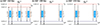 |
Fig. 1. Energy levels of Si+ ions and different channels of excitation and de-excitation from the ground-state or the fine-structure level (fluorescence) for Si II* λ1265, 1309, 1533 lines in panels (a) to (c), respectively. The probabilities (P) of related transitions and their wavelengths are also shown. The ionization energies of these LIS lines are close to that of H I. The Si II* lines can be regarded as an escape channel of photons from Si II resonant scattering. |
Fluorescent lines are extremely faint, and Si II* emission is ∼10–50 times weaker than Lyα emission of LAEs (Steidel et al. 2018). Extended Si II* emission has not been directly detected. Wang et al. (2020) found weak Si II* emission lines compared to the associated absorption line in HST/Cosmic Origins Spectrograph (COS) data for five galaxies at z = 0, which implies that the bulk of Si II* emission arises on larger scales than the COS aperture. Gazagnes et al. (2023) compare COS spectra of Si II* λ1265 for 45 local galaxies (COS Legacy Archive Spectroscopic SurveY, CLASSY) with mock spectra from zoom-in simulations (Mauerhofer et al. 2021). They find stronger Si II* emission lines in the simulations than observed, and they argue that aperture losses of COS can explain the weakness of observed Si II* and that Si II* λ1265 is spatially extended. Very recently, Keerthi Vasan et al. (2024) studied spatially resolved outflow properties for a lensed star-forming galaxy at z = 1.87 with KCWI, and show that Si II* emission is more extended than the continuum for a certain direction extracted with a pseudo slit.
For this project, we searched for Si II* halos around galaxies at cosmic noon (at z = 2–4) as a tracer of metal-enriched cool CGM using integral field unit data to remedy the problem. We used data from the MUSE Hubble Ultra Deep Field (HUDF) survey (Bacon et al. 2023) and tested the presence of Si II* halos with surface brightness profiles of Si II* and UV continuum. We report the first detections of Si II* halos. We also stacked the MUSE data for a UV-bright subsample to study the general extent of Si II* and compared it with simulations.
The paper is organized as follows. In Sect. 2 we describe the data and the sample construction. Section 3 presents methods and results of the search for individual Si II* halos and those of a stacked subsample. In Sect. 4 we discuss photon conservation for Si II, compare observed results with those of zoom-in simulations, and discuss how to increase a sample size with different selection criteria. Finally, conclusions are given in Sect. 5. Throughout this paper, we assume the Planck 2018 cosmological model (Planck Collaboration VI 2020) with a matter density of Ωm = 0.315, a dark energy density of ΩΛ = 0.685, and a Hubble constant of H0 = 67.4 km s−1 Mpc−1 (h100 = 0.67). Magnitudes are given in the AB system (Oke & Gunn 1983). All distances are in physical units (kpc), unless otherwise stated.
2. Data and sample
To search for extended Si II* emission of z ≳ 2 galaxies, we utilized deep MUSE data from data release 2 (DR2) of the MUSE HUDF surveys (Bacon et al. 2023), where rich multiwavelength data are also available (see Sect. 2.1). We constructed our sample with the DR2 catalog using the systemic redshifts for the individual search and stacking analyses (see Sects. 2.2 and 2.3). We created masks to avoid potential contaminations from neighboring galaxies (see Sect. 2.4).
2.1. Data and catalogs
The MUSE HUDF DR2 data were obtained as a part of the MUSE guaranteed time observations (GTO) program described in Bacon et al. (2023). We used two fields among the MUSE HUDF DR2 data set: a single 1 × 1 arcmin2 pointing with a 31-hour depth (udf-10; see also Bacon et al. 2017 and Inami et al. 2017), and the adaptive-optics (AO) assisted MUSE eXtremely Deep Field (mxdf), whose maximum integration time is 141 hours with a 1 arcmin diameter field of view. They are located inside the Hubble eXtreme Deep Field (XDF; Illingworth et al. 2013) with deep HST data (see Bacon et al. 2023, for more details). The mxdf is the deepest IFU survey ever performed, while the udf-10 is the second deepest available for this study, which has multiwavelength data and catalogs constructed in the same manner as mxdf. The udf-10 covers the optical wavelength range from 4750 Å to 9350 Å, while mxdf covers from 4700 Å to 9350 Å, with an AO gap from 5800 Å to 5966.25 Å. The spectral resolving power of MUSE varies from R = 1610 to 3750 at 4700 Å to 9350 Å, respectively. The full widths at half maximum (FWHMs) of the Moffat point spread function (Moffat PSF, Moffat 1969) are  (
( ) at the blue wavelength edge and
  (
( ) at the red wavelength edge for the mxdf (udf-10). The 3σ point-source flux limit for an unresolved emission line in the mxdf (the udf-10) is ≃6 × 10⁻²⁰ erg s−1 cm−2 (≃2 × 10⁻¹⁹ erg s−1 cm−2), at around 7000 Å (not affected by OH sky emission), which corresponds to a 3σ surface brightness limit for an unresolved emission line of ≃1 × 10⁻¹⁹ erg s−1 cm−2 arcsec−2 (≃2 × 10⁻¹⁹ erg s−1 cm−2 arcsec−2; see Bacon et al. 2023).
The MUSE HUDF DR2 catalog includes 2221 sources from z = 0 to 6.7, which were selected by emission-line detections and through HST priors. The details of the catalog construction are described in Bacon et al. (2023). Each MUSE object has a source file, which is in the format of MPDAF2 multifits format and is composed of various data files such as minicubes, images, and spectra. It is available on the AMUSED website3. We used 5′′ × 5′′ minicubes from each of the source files. We created continuum-subtracted minicubes following the method used in Kusakabe et al. (2022), taking the median for each pixel within a spectral window of 100 slices (masking ±400 km s−1 around the Lyα wavelength if the spectrum covers). The continuum subtraction is useful not only to investigate emission lines, but also to remove neighboring sources around a target source. In order to identify the HST counterparts, calculate UV magnitudes, and create masks, we used the HST catalog and data from Rafelski et al. (2015).
2.2. Sample selection
We constructed a sample of galaxies at z = 2.07–3.87, for which the [C III]λ1907, C III]λ1909 doublet nebular lines and at least one of the Si II* λ1265, 1309, 1533 lines are redshifted into the MUSE wavelength range. The available redshift ranges for the three Si II* lines are shown in the top panel in Fig. 2. We required sources to have a secure spectroscopic redshift with ZCONF ≥ 2 and a C III] signal-to-noise ratio (S/N) of S/N > 3. We visually inspected C III] in spectra and images extracted from MUSE cubes to ensure these criteria. We used systemic redshifts measured by the C III] line rather than reference redshifts (REFZs) in the DR2 catalog, which are given by Lyα at z ≳ 3 or absorption lines at z ≃ 2. Si II* lines are expected to be located at the systemic redshifts (e.g., France et al. 2010; Dessauges-Zavadsky et al. 2010; Jaskot & Oey 2014; Wang et al. 2020), though redshifted Si II* lines are also reported, which could be due to the contamination of the absorption at the blue edge for low-resolution spectra or stacking of spectra for different sources (e.g., Shapley et al. 2003; Erb et al. 2010; Berry et al. 2012). As Si II* lines are extremely faint, secure measurements of systemic redshifts enable us to not rely on the presence of Si II* in 1D spectra on a galaxy scale and to directly search for spatially extended Si II* in narrowband images extracted from MUSE cubes. We limited our sample to galaxies with a secure and isolated HST counterpart (based on Rafelski et al. 2015, MAG_SRC = RAF) with a high HST matching confidence level of MCONF ≥ 3 in the DR2 catalog. In total, we have 39 galaxies, which are summarized in Table A.1. Absolute UV magnitudes (MUV) and systemic redshifts (zsys) are shown in the middle panel of Fig. 2. The MUV is calculated at rest-frame 1600 Å by fitting two or three HST bands with a power-low model (with parameters being an amplitude and a UV slope β). Figure 2 also indicates the redshift coverage of the three Si II* lines (top panel) and the surface brightness limits for each field (bottom panel). The stellar masses and star formation rates (SFRs) of the sample are shown in Fig. A.1.
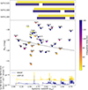 |
Fig. 2. Redshift distribution of our sample. (Top) Redshift ranges covered for the Si II* λ1265, 1309, and 1533 lines. Dark blue and yellow indicate mxdf and udf-10, respectively. The gaps between the dark blue bars are the AO gap (see Sect. 2.1). (Middle) MUV and zsys distribution of our sample with MUSE IDs. The color bar at the right indicates the integration time. The stacked subsample is enclosed by gray squares. The MUV corresponding to mUV = 26.0 (magnitude cut for the stacking sample) at each redshift is shown by the black dashed line. The individually detected Si II* halos are indicated by red crosses (see Sect. 3.2 ). (Bottom) 1σ SB limits for Si II* λ1533 in mxdf (dark blue) and udf-10 (yellow), which are converted from the median surface brightness limits on the sensitivity table in Bacon et al. (2023) using the narrow band widths for Si II* λ1533 for given redshifts (see Sect. 3.1). The Si II* halos tend to have bright MUV. |
We would like to note that our sample was constructed simply with the deepest data for this pilot study. We discuss possible strategies to extend the sample in Sect. 4.3.
2.3. Stacked sample
The subsample used for the stacking analysis is restricted to bright UV-continuum galaxies using an apparent magnitude cut of mUV = 26.0, in order to enhance the S/N of the stacked images (see Sect. 3.3 and Fig. 2). The origin of Si II* is predicted to be continuum pumping, as mentioned in Sect. 1, and a bright UV continuum is necessary to have a bright Si II* emission line. The Si II* emission lines are stronger in 1D stacked spectra for subsamples of MUSE LAEs with brighter UV continuums (such as those with higher stellar masses and with brighter UV magnitudes) than the subsample counterparts in Feltre et al. (2020). The number of sources for the stacking subsample is 14. We note that applying fainter magnitude cuts reduces the S/Ns of the Si II* lines.
2.4. Masks
In order to exclude pixels that might be affected by bright neighboring objects in Si II* narrowband images extracted from the minicubes, we created neighboring object masks. First, we defined target pixels. We used an HST segmentation map and masked pixels not corresponding to a main target on a 5′′ × 5′′ HST/F775W cutout for each object. It was convolved with the MUSE moffat PSF at the redshifted Si II* wavelength for the main target and rebinned to match the MUSE pixel scale. Then, we applied a threshold value of 0.1 to the peak-normalized convolved cutout to delimit the spaxels of the target. Lower threshold values such as 0.05 cause contamination of neighboring objects inside the target spaxels. Using a higher threshold value of 0.2 does not change the main results in this paper, but enhances the contaminated pixels outside the following neighboring object masks. Therefore, we adopted the value 0.1.
Second, we used a 5′′ × 5′′ HST/F775W cutout whose sky and the main target were masked with the HST segmentation map for each source. This cutout was convolved with the MUSE PSF and rebinned to match the MUSE pixel scale. Then, we defined pixels brighter than a certain threshold on the cutout, except for the target pixels, as masked pixels. The applied threshold value was half of the value above in the absolute sense (without normalization).
3. Results
3.1. Extracted images and surface brightness profiles
For each source we created a Si II* emission narrowband (NB) image from the continuum-subtracted minicube. We summed fluxes in a window of ±200 km s−1 around the Si II* wavelength, excluding NaN (masked) spaxels, wavelength slices affected by OH skylines, and the AO gap in the cube. The variance image of the NB was created from that of the cube with error propagation. A UV continuum broadband (BB) was created from the median filtered original minicube with a window of ±300 wavelength slices (375 Å) around the Si II* wavelength (masking below +400 km s−1 from the Lyα wavelength) to obtain a good S/N. We also excluded NaN in the cube and the AO gap. If the wavelength window was not fully covered, we used as many spectral slices as possible. The variance image of the BB was assumed to be identical to that of the mean-filtered BB created from the same cube with error propagation. We applied a neighboring object mask (see Sect. 2.4) and measured SB profiles of these two bands using PHOTUTILS (Bradley et al. 2021). The aperture and annuli were centered at the HST counterpart position with 1 pixel ( ) annuli from
  to
to  , then 2 pixel annuli at
  and
and  , followed by a 3.5 pixel annulus at
  , to enhance the S/N at outer radii. The azimuthally averaged radial SB profiles were calculated from the effective areas and the measured flux above. We normalized the SB profile of the UV continuum at the innermost radius (R =
  ) to that of Si II*.
The top panels in Fig. 3 show the Si II* emission NB, the UV-continuum BB, and the SB profile for a highlighted object, MID = 1141. The details of this object are explained in Sect. 3.2.
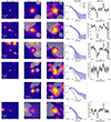 |
Fig. 3. Images and spectra for Si II* halos. (From left to right) The HST image, MUSE UV-continuum BB image, MUSE Si II* NB image, SB profile, and Si II* spectrum for the five sources with Si II* halo detections. Each row (except the fifth) shows the Si II* λ1533 line for a different object. The fifth row shows a coadded result of three Si II* lines for MID = 50 at z = 3.32, whose three Si II* lines (Si II* λ1265, Si II* λ1309, and Si II* λ1533) are covered with MUSE. The image size is five arcsec. The gray shades indicate masked spaxels. For presentation purposes, NB images are smoothed with a Gaussian kernel with σ = 1.5 spaxel. The white contours correspond to 1 × 10⁻¹⁹ erg s−1 cm−2 arcsec−2 (the typical 3σ SB limit in MXDF for an unresolved emission; Bacon et al. 2023). The cyan crosses indicate the HST center. The SB profiles of the UV continuum (black lines) are normalized at the innermost radius (R = |

3.2. Identification of Si II* halos
To identify extended Si II* emission, we compared the shape of the azimuthally averaged radial SB profiles of the UV continuum and the Si II* emission. We took account of uncertainties in SB profiles of Si II* emission only (blue shades in Fig. 3) as those of the UV continuum are negligibly small (gray shades). If more than two adjacent data points of the Si II* SB profiles deviated by more than 1σ from the normalized continuum, we identified it as extended Si II*. The significance of the presence of the halo with this criterion corresponds to more than 97.5%4. As we used circular photometry, we note that our test may have missed noncircular halos, as discussed in Kusakabe et al. (2022) for Lyα halos. Developing and testing noncircular methods requires high S/N objects for reliable assessments, which our sample was not eligible for. Our halo search was not complete in that sense, but it was secure.
Among the 39 sources, we detected five Si II* halos for the Si II* λ 1533 line (MID = 24, 35, 50, 51, 1141; see Fig. 3). These are the first detections of individual Si II* halos. The Si II* lines in the DR2 reference spectra show that there are no significant velocity shifts for the line peaks of the Si II* λ1533 (Fig. 3; the systemic redshifts are given by the [C III] λ1907, C III] λ1909 doublet nebular lines; see Sect. 2.2). Meanwhile, peaks of the Si IIλ1527 absorption lines show velocity offsets, which have often been observed in the down-the-barrel analysis and interpreted as gas flows (e.g., Du et al. 2018)5.
Among the five Si II* halo sources, MID = 1141 (shown in the top panels of Fig. 3) is the best-case object. The Si II* emission profile shows three data points that deviate by more than 1σ from the normalized continuum. This object is well-isolated and without a spatial offset of Si II* from the UV continuum. The images are not significantly affected by masks, which makes the SB profile test secure. The Si II* emission line can be clearly confirmed on the spectrum shown in Fig. 3. MID = 24 and MID = 35 are a pair of galaxies that could contaminate each other’s 5′′ × 5′′ images despite the neighboring object mask. Moreover, MID = 35 is an X-ray detected AGN (Luo et al. 2017), whose Si II* halo might have a different origin from other sources. The Si II* NB of MID = 50 shows a peak offset from the UV center measured with the HST data, with two neighboring LAEs in the DR2 catalog, which spatially overlap with the extended Si II* emission. The Si II* SB of MID = 51 is noisy even though it meets our halo criterion. Considering these details on the five sources, we highlight MID = 1141 in the following sections.
As shown in Fig. 2, the five individual halos tend to have bright UV magnitudes, which is qualitatively consistent with the continuum pumping scenario of Si II* emission. We also show the possible differences in SFRs and M⋆ between Si II* λ1533 halo sources and nondetected sources in Fig. A.1, and also examine the dependence of detections of halos on 1σ SB limits for Si II* NBs in Fig. B.1, although this discussion is beyond the scope of this paper. Overall, due to the small sample size, we cannot draw these conclusions, but the UV magnitudes and redshifts of the sources might be essential.
The redshifts of the individually detected Si II* λ1533 halos range from 2.23 to 3.32 with four of them at zsys ≲ 2.5. The nondetections at z > 3.5 would be caused by the lack of UV-bright sources (see Figs. 2 and B.1) if the origin of Si II* is continuum pumping. It could also be due to the high noise levels of MUSE data at red wavelengths (severe night sky and low sensitivity; Bacon et al. 2023) and the cosmic dimming effect on the SB profiles (by a factor of 2.7 between z = 2.5 and z = 3.5). In the case that the circumgalactic Si II* is intrinsically fainter at z ∼ 2 than at z > 3.5, it implies a rapid evolution of metal enrichment in the CGM, which is qualitatively consistent with the redshift evolution of the number density of Mg II absorbers (Matejek & Simcoe 2012; Zhu & Ménard 2013) as well as the prediction from a chemical evolution model with UniverseMachine (Behroozi & Silk 2018; Nishigaki et al. in prep.).
Another interesting result is that we cannot confirm extended emission for any of the other Si II* lines (λ1265, 1309). In the optically thin limit, the strengths of the fluorescent lines are expected to depend on the strengths of the paired absorption lines, which are determined by their oscillator strengths, f. In particular, the Si IIλ1260 resonant absorption line corresponding to the Si II* λ1265 line has a ten times higher f than that of the Si IIλ1527 resonant absorption line corresponding to the Si II* λ1533. However, in the simulations of Mauerhofer et al. (2021) there is no significant difference in the equivalent widths (EWs) of Si II* λ1265 and Si II* λ1533 absorption lines because both lines are saturated (Mauerhofer et al. in prep.). In such an optically thick regime, the equivalent widths for the corresponding fluorescent emission (Si II* λ1265 and Si II* λ1533) are similar in the simulations. Therefore, nondetections of Si II* λ1265 and Si II* λ1309 would not be due to fainter total fluxes for these lines than for the 1533 line. The reason for the nondetections of the Si II* λ1265 and Si II* λ1309 halos is not clear. The samples for Si II* λ1265, 1309 lines are limited to high redshifts (zsys > 2.8 and > 2.6, respectively), and none of them are bright in apparent UV magnitudes, which are directly related to S/N values (see Fig. 2). Bright sources would be crucial for the detection of diffuse Si II* lines if the origin of Si II* were continuum pumping. However, we cannot distinguish whether it is caused by differences in lines, samples, or noise levels. We note that the Si II* λ 1533 lines are also brighter than the other two lines in the stacked MUSE LAE spectra of Feltre et al. (2020) and Kramarenko et al. (2024), which might also be due to the difference in objects stacked for different Si II* lines.
One of the individually detected objects, MID = 50 at zsys = 3.32, has three Si II* lines covered with MUSE. We coadd the NBs and BBs for the three Si II* lines by taking the median (with the same method as used in Sect. 3.3) and show them in the fifth row of Fig. 3. Extended Si II* is confirmed with a better S/N, which implies that the Si II* λ1265, 1309 lines are also spatially extended.
3.3. Stacking analysis
To test the general presence of Si II* halos, we stacked 14 UV-bright sources (see Sect. 2.3). The numbers of sources with the magnitude cut of mUV = 26.0 available for each of the Si II* λ1265, 1309, and 1533 lines are 5, 4, and 13, respectively, which are limited by the MUSE wavelength coverage and the AO gap (see Fig. 2)6. Therefore, we only stacked a subsample for the Si II* λ1533 line and took the mean and median of the Si II* NBs and BBs without weighting, while masking neighboring objects. We also stacked 14 sources by combining the NBs and BBs for the three lines. The variance images for the mean stacking, which we used for our halo test, were created based on error propagation. Then, we applied the SB profile test for the mean-stacked images with the same method as described in Sects. 3.1 and 3.2, as the uncertainties can be calculated correctly for the mean, but not for the median.
The results of this stacking experiment are shown in Fig. 4. As shown in the top row, we confirm the existence of a Si II* λ1533 halo with five data points that deviate by more than 1σ from the normalized continuum profile. The median profile of Si II* λ1533 is consistent with the mean profile and deviates from the median continuum as well, in particular at large radii. These tests may suggest that the detected halo in the mean profile is not dominated by a few extreme objects. This is the first secure detection of a stacked Si II* halo. It may imply that the individually detected sources are not extreme cases, and that Si II* halos must be common for UV-bright galaxies at z = 2–4.
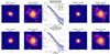 |
Fig. 4. Stacking results. From left to right, we show the mean-stacked UV continuum image, the mean-stacked Si II* emission image (5 arcsec each), the mean surface brightness profiles, the median-stacked UV continuum image, and the median-stacked Si II* emission image. The top and bottom panels represent stacking results of the Si II* λ1533 line (N = 13) and those of all Si II* lines (22 images for 14 sources), respectively. The cyan crosses indicate the HST center. The white contours correspond to 5 × 10⁻²⁰ erg s−1 cm−2 arcsec−2, which is also shown by black dotted lines on the SB profiles. The SB profiles of the mean-stacked Si II* and UV continuum are indicated by the blue and black lines, respectively, while the median-stacked Si II* and UV continuum are shown by the blue and the black crosses, respectively. The blue and gray shades represent 1σ uncertainties of the SB for Si II* emission and UV continuum, respectively. Following Fig. 3, the SB profiles for the continuum are normalized at the innermost radius (R = |

The bottom row of Fig. 4 shows the results of stacking all the Si II* narrowbands and corresponding UV continuum bands for the 14 sources (three lines; in total 22 images). We find that the mean-stacked Si II* deviates by more than 1σ from the mean-stacked UV continuum for six data points. The median-stacked Si II* is consistent with the mean-stacked Si II*, and the deviation from the normalized continuum is similarly seen with the median-stacked profiles.
We note that removing MID = 35, which is an X-ray detected AGN with extended Si II* (see Sect. 3.2), does not change the results, and that the other 13 sources do not have a counterpart in the deep X-ray catalog (Luo et al. 2017). We also note that stacking without individually detected Si II* halos results in nondetections of extended Si II*. As shown in Fig. 2, all the individually detected sources have a bright MUV (and also a bright mUV) and are located at relatively low redshifts. It is not surprising that removing these five sources results in nondetections. If the origin of the Si II* is continuum pumping, as we expect, it should then be more challenging to detect Si II* halos without these bright sources. We also stacked various subsamples including all the sources without individually detected halos and obtained nondetections of extended Si II* emission. Future instruments such as BlueMUSE (Richard et al. 2019) or a larger sample compiling MUSE and KCWI archive data will allow us to investigate the dependence of Si II* halos on sample properties such as MUV (see Sect. 4.3). It will enable us to draw a firm conclusion on whether Si II* halos are common for UV-bright galaxies at z = 2–4 or not.
4. Discussion
4.1. Testing photon conservation
Shapley et al. (2003) suggested that the origin of the Si II* is continuum pumping (see Sect. 1 for other origins). For the Si II* λ1533 line, Si+ in neutral clouds makes a Si IIλ1527 resonant absorption line, and then a fraction of Si+ de-excites to the fine-structure level, emitting Si II fluorescence photons at 1533 Å (see Fig. 1). As the Si II is a resonant line, the Si II* line can be regarded as an escape channel of photons from resonant scattering. When dust opacity is high in the ISM and the CGM, dust attenuation for Si II* can be greater than that for the UV continuum, depending on the number of scatterings. If the additional dust attenuation of Si II* is negligible and the escape is isotropic, then the EW of Si II* emission and that of the corresponding resonant absorption should be comparable because of photon conservation.
However, it is possible for the absorption and emission to have different EWs for one given direction of observations, even if the origin is continuum pumping without dust, because of the complex gas distribution in front of stars in galaxies (e.g., Prochaska et al. 2011b; Carr et al. 2018). The simulations predict that absorption lines depend sensitively on the direction of observations (Mauerhofer et al. 2021; Gazagnes et al. 2023). Below, we assume an isotropic case.
To investigate the scenario of continuum pumping, we used the isolated high S/N object MID = 1141 (see Sect. 3.2) and tested photon conservation between Si II absorption and associated Si II* emission, which is commonly assessed with the EWs of these lines (e.g., Prochaska et al. 2011a; Wang et al. 2020). First, we checked the flux curve of growth (CoG) for the continuum and the emission line to determine the spatial extent. Second, we measured the EW curve of growth for Si II* emission and compared it with the absorption EW. We measured EWs from the MUSE data (without HST), which makes the EW comparison fair. Ideally, we should measure the curve of growth for the absorption. However, due to the limited depth and spatial resolution of our data, we have to assume that the absorption follows the same spatial profile as that of the continuum. The left panel of Fig. 5 shows normalized fluxes within growing apertures for continuum (black) and Si II* λ1533 (blue). The fluxes were measured from the Si II* λ1533 NB image and the corresponding UV continuum BB image (Sect. 3.1) with PHOTUTILS and the neighboring object masked with corrections of masked areas. On a galaxy scale of  , the aperture includes about 80% of the continuum, but only 50% of the Si II*. An
  aperture captures most of the Si II* flux.
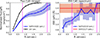 |
Fig. 5. Curve of growth (CoG) for Si II* flux and EW for MID = 1141. Left: Normalized fluxes within radius R as a function of R measured from the Si II* NB image (blue line) and the UV continuum BB image (black line). The blue shade indicates 1σ uncertainties for the Si II* flux. The vertical magenta lines show R = |


The right panel shows the rest-frame EWs for Si II* λ1533 emission within growing apertures (blue), compared with the EW for Si IIλ1527 absorption measured at  , EWabs(Si IIλ1527) = 1.6 ± 0.2 Å (red). Rest-frame EWs were measured in spectra extracted from the original minicube (to which the neighboring object mask was applied) with growing apertures. The continuum flux density was measured by the median filtering each spectrum from 50-slice shorter wavelength (62.5 Å) than the absorption to 50-slice longer wavelength than the emission. The absorption and emission fluxes were measured as differences from the continuum. The EW for Si II* λ1533 is EWem(Si II* λ1533) = 1.1 ± 0.1 Å at
  , which is smaller than EWabs(Si IIλ1527) = 1.6 ± 0.2 Å. EWem(Si II* λ1533) increases with R and reaches EWem(Si II* λ1533) = 1.8 ± 0.4 Å at
  , which is consistent with EWabs(Si IIλ1527) at
  within the 1σ uncertainties (see Fig. 6 for the spectra), although the EWs have large measurement errors. Therefore, the absorption EW on the galaxy scale and the fluorescent emission EW on the CGM scale are consistent with each other. This is compatible with photon conservation on the CGM scale, albeit with large uncertainties. It implies that the origin of extended Si II* emission can be continuum pumping, as predicted under the assumption of isotropic escape and no dust. In that case, either a small amount of dust, a low optical depth, or a combination of both are implied. Unfortunately, data for the other four sources with individual Si II* halos are either noisy or have accompanying galaxies inside their 5′′ × 5′′ minicubes, which prevents us from obtaining a firm conclusion about the mechanisms for the four sources. The trend of increasing EW of Si II* emission with radius beyond the galaxy scale is predicted by simulations (Mauerhofer et al. 2021), which are compared with the slit spectroscopy of low-redshift galaxies in Gazagnes et al. (2023, see also Wang et al. 2020).
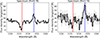 |
Fig. 6. Galaxy-scale and CGM-scale spectra for MID = 1141. Left: Spectrum extracted from the original minicube (black line) with a |


4.2. Comparisons with zoom simulations
Here we compare our stacked Si II* λ1533 profile with those from the cosmological zoom-in simulations of Mauerhofer et al. (2021), which are used in Gazagnes et al. (2023) and Blaizot et al. (2023). Mauerhofer et al. (2021) present three snapshots containing a relatively small galaxy (such as MUSE LAEs) at z = 3.0, 3.1, and 3.2. The stellar mass for the simulated galaxy is M⋆ ∼ 2 × 10⁹ M⊙, which is similar to the median value for the 14 galaxies used in the stacking analysis, M⋆ ∼ 3 × 10⁹ M⊙ (ranging M⋆ ∼ 1 × 10⁹–2 × 10¹⁰ M⊙, Bacon et al. 2023, see Fig. A.1). The SFRs of the simulated galaxy for the three snapshots are 2.2 M⊙ yr−1, 4.2 M⊙ yr−1, and 5.0 M⊙ yr−1, which are similar to the median value of the observed galaxies, 3.4 M⊙ yr−1 (ranging SFR = 1.5–24.5 M⊙ yr−1; Bacon et al. 2023, see Fig. A.1). The Si II* photons in these simulations originate from continuum pumping. We provide mock MUSE cubes for observations from 12 directions for each snapshot in the rest frame. This original mock cube has a size of 300 × 300 × 110 pixels corresponding to  Å (from 1521.83 Å to 1538.42 Å) with a spaxel scale of
  /pix. Then, to match the size of the observed and simulated galaxies, we measured the median size of the simulated galaxy from the 36 directions. A UV-continuum BB image is created from each median-filtered original cube with a window from 1528.5 Å to 1531.5 Å (the continuum between Si II absorption and Si II* emission). We defined the galaxy center by identifying the brightest pixel, as in Gazagnes et al. (2023), for each UV continuum BB image after HST PSF convolution (F606W in Rafelski et al. 2015). The half-light radius (R50) was measured around the galaxy center with the original mock cube (without HST PSF convolution) using PHOTUTILS. The median R50 for the simulated galaxy is
  (3.5 pix). This is 1.7 times smaller than the median R50 for the 14 stacked galaxies (
 with F606W after PSF correction). Since we did not have a simulated galaxy that is large enough in Mauerhofer et al. (2021), we manually rescaled the original mock cube by a factor of 1.7 by interpreting the spaxel scale as
  /pix, which is referred to as an intrinsic mock cube below. The intrinsic mock cubes were cut out around the galaxy center defined above and are 5 arcsec each. The 5″ cubes were convolved with the MUSE PSF and line spread function (LSF) described in Bacon et al. (2023) at the median redshift of the stacked sample (z = 2.68). Then the convolved mock cubes were rebinned to match the MUSE cubes in the rest frame. We applied similar analyses to the 36 mock MUSE cubes used for the observational data (see Sect. 3). A slight difference from the method for the MUSE data is continuum subtraction. Continuum cubes used for continuum subtraction were created using median filtering from 1528.5 Å to 1531.5 Å, which were also used for the UV-continuum BB images. The 1σ uncertainties for stacked mock data were derived from 15.87 to 84.12 percentiles of SB profiles among individual mocks. We note that the simulations assume the cosmological parameters of H0 = 67.11 km s−1 Mpc−1 and Ωm = 0.3175, which should not have a significant impact on the results below. We converted distances in units of arcseconds for the simulated data into kiloparsec at z = 2.68 with the Planck 2018 cosmological model (Planck Collaboration VI 2020) as the galaxy sizes are matched and MUSE PSF are convolved in units of arcseconds.
The left panel of Fig. 7 shows a comparison of the observed and simulated mean-stacked SB profiles. The simulated UV continuum (gray dotted line) is well matched with the observations (black solid line), thanks to our manual 1.7 times expansion. The simulated Si II* λ1533 profile (green dotted line) is more extended than the simulated UV continuum (gray dotted line) and consistent with the observed Si II* λ1533 (blue solid line), though the simulated Si II* halo is slightly less extended than the observed halo within 1σ uncertainties.
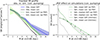 |
Fig. 7. Stacked SB profiles of our observations and of zoom-in simulations from Mauerhofer et al. (2021). Left: Comparison of stacked SB profiles. The blue and black solid lines show the observed mean-stacked SB profiles of Si II* λ1533 and the continuum, respectively. The blue shade indicates 1σ uncertainties for Si II* λ1533. The observed continuum is normalized at R = 0 to the peak of the observed Si II* λ1533. The green and gray dotted lines (shades) show the mean-stacked SB profiles of Si II* λ1533 and the continuum, respectively, for the simulations after PSF and LSF convolution (their 1σ uncertainties, which correspond to the 15.87 to 84.13 percentiles of SB profiles for individual mocks). They are normalized at R = 0 to the peak of the observed Si II* profile. Right: Stacked SB profiles for simulations. The green and gray dotted (solid) lines show the mean-stacked SB profiles of Si II* λ1533 and continuum, respectively, with (without) PSF and LSF convolution. The green and gray crosses show the median-stacked SB profiles of Si II* λ1533 and the continuum, respectively, with PSF and LSF convolution. They are scaled by the same factor as used in the left panel. The left panel shows that the observed stacked SB profiles can be reproduced within the 1σ uncertainties by the simulations, which account for continuum pumping. |
The mean profiles can be biased toward bright halo sources, so we checked whether the mean-stacked profiles are consistent with the median-stacked profiles for the Si II* and the continuum (green and gray crosses, respectively; see the right panel of Fig. 7). We confirm that they are consistent with each other, as for the MUSE observations of Si II* λ1533. The right panel also compares simulated mean-stacked SB profiles with PSF and LSF convolution versus without convolution, indicated by the dotted and solid lines, respectively. The simulated galaxy has significantly more extended Si II* λ1533 than the UV continuum in the intrinsic mock cubes, but the difference is mostly hidden by the MUSE PSF convolution7.
We also checked the EW CoG of Si II* λ1533 emission and Si IIλ1527 absorption lines for the simulations, as shown in the left panel of Fig. 8. The EWs of Si II* λ1533 emission and Si IIλ1527 absorption are consistent at a CGM scale for both intrinsic cubes and PSF-convolved cubes, which are also seen in the mock spectra (see the middle and right panels of Fig. 8). This means that the photon conservation works for the simulations with continuum pumping, in the sense that the scattered photons are not more attenuated by dust than the stellar continuum. This is consistent with our observations for MID = 1141.
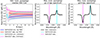 |
Fig. 8. EW CoG and spectra of the simulations with continuum pumping. Left: Median cumulative EW in rest-frame as a function or R. The blue and red solid lines (shades) indicate the EW of Si II* λ1533 emission and Si IIλ1527 absorption lines (their 1σ uncertainties) with MUSE PSF convolution, respectively. The cyan and magenta dashed lines (shades) show the intrinsic EW of Si II* λ1533 emission and the Si IIλ1527 absorption lines (their 1σ uncertainties). Middle: Median spectrum extracted from the intrinsic mock cube with a 1.2 kpc aperture (galaxy scale) shown by the black line. The cyan and magenta lines show the wavelength of Si II* λ1533 emission and Si IIλ1527 absorption lines, respectively. Right: Median spectrum extracted from the intrinsic mock cube with a 19 kpc aperture (CGM scale). The EWs of the Si II* λ1533 emission and Si IIλ1527 absorption are consistent on a CGM scale for both intrinsic cubes and PSF-convolved cubes, which are also seen on the mock spectra. |
From these comparisons, we conclude that our simulations with the continuum pumping scenario can reproduce the observations. This lends additional support for the interpretation of Si II* emission as a signature of continuum pumping. We note that the selection bias with the UV magnitude cut may have an impact on the observed result and this comparison. The mock observations are re-scaled by a factor of 1.7 to correct for the fact that the simulated galaxy is smaller than the observed ones (see above). The simulated galaxy is fainter than the observed one, though the range of absolute magnitudes overlaps (MUV from −18 to −19). It would be interesting to test the selection bias with a larger and brighter simulated galaxy, or several, perhaps at a slightly lower redshift.
4.3. Possible extension of the sample
In this section we discuss the possible strategies to extend the sample with the existing data. There are a few ways to increase the sample size: (1) using sources at z > 3.87, which have other nebular line detections such as the O III] λλ1661, 1666 doublet, and He IIλ1640 in the same catalog and the same field (with the same integration time), (2) using sources located in shallower fields, such as mosaic field (9 × 9 pointing with ten-hour integration, in the same catalog as Bacon et al. 2023) and MUSE-WIDE field (one-hour integration Herenz et al. 2017; Urrutia et al. 2019; Kerutt et al. 2022), (3) using UV-bright sources at the same redshifts in other fields with similarly long integration times (> 30 hours) in the MUSE archival data (e.g., Fossati et al. 2019; Lofthouse et al. 2020). Samples (1) and (2) were tested with the MUSE DR2 catalog (not including MUSE WIDE) in the same manner. We find that these less restrictive selection criteria do not help increase the number of detections of Si II* halos. Therefore, method (3) using deep MUSE archival data for UV-bright galaxies with the same selection criteria would be the best way to extend the sample in the future.
There are some additional ways to increase the sample size: (4) using gravitationally lensed sources observed with MUSE (e.g., Richard et al. 2021; Claeyssens et al. 2022, Claeyssens et al. in prep.) would be useful to investigate more compact Si II* halos in the future (see the right panel of Fig. 7), which would be hidden by the PSF without the power of the magnification. We note that they are not included in this pilot study as magnification can add complications and uncertainties. To investigate Si II* halos at higher redshifts (z ∼ 3–6), whose Si II* lines are covered with MUSE, is possible (5) using sources with systemic redshifts measured by nebular lines with JWST, and (6) using MUSE LAEs, whose systemic redshifts can be estimated by empirical relationships based on the Lyα line (Verhamme et al. 2018). We do not include these sources in this pilot study, considering uncertainties in wavelength calibration (e.g., Maseda et al. 2023; D’Eugenio et al. 2024; Meyer et al. 2024) and more severe cosmic dimming effects. We leave the investigation of higher-z sources to a future work.
5. Conclusions
To study the spatial distribution of the metal-enriched cool CGM at cosmic noon in emission, we search for extended Si II* emission (fluorescent lines) using the MUSE HUDF data and catalog with 30–140 hour integration times. We construct a sample of 39 galaxies with systemic redshifts at z = 2.07–3.87, at which the [C III]λ1907, C III]λ1909 doublet nebular lines and at least one of the Si II* λ1265, 1309, 1533 lines are redshifted into the MUSE wavelength range. Our major results are summarized as follows:
-
Five individual Si II* λ1533 halos are confirmed to be present from statistical tests with surface brightness profiles. These are the first detections of extended Si II* emission.
-
We stacked images of the Si II* λ1533 line for a subsample of 13 UV-bright galaxies. We confirm the presence of stacked Si II* λ1533 halos, which may imply that metal-enriched CGM is common for UV-bright galaxies. We also stacked images of Si II* λ1265, 1309, and 1533 for 14 UV-bright galaxies and detected a Si II* halo. If we stack fainter galaxies or remove the five individually detected halos from the stacking, we get nondetections of Si II* halos. We need a larger sample to draw a firm conclusion.
-
We find that the EW of the absorption line and fluorescent emission line are roughly equal when integrated out to large distances for MID = 1141. This suggests that photons are conserved and that the emission line is mostly due to pumping from the stellar continuum.
-
We tested for the presence of Si II* halos in zoom-in simulations, which account only for continuum pumping. After re-scaling the mock observations to correct for the fact that the simulated galaxy is smaller than the observed one, we find that the simulated halos are consistent with the observed stacked halo within 1σ uncertainties. This trend gives additional support for the interpretation of Si II* emission as a signature of continuum pumping.
-
The best way to extend our sample with existing data in the future is using deep MUSE and KCWI archival data for UV-bright galaxies with the same selection criteria.
KCWI or BlueMUSE (Richard et al. 2019) will allow us to investigate HI Lyα halos for Si II* halos detected with MUSE. BlueMUSE will also make it possible to individually detect Si II* halos of more diverse sources and to study their statistical properties thanks to a more moderate cosmic dimming effect at z ≃ 2 (by a factor of three, compared to z ≃ 3). These larger samples would be useful to improve the stacking experiments (see also Sect. 4.3) and to study spectral variations at different radii from the centers of galaxies as done for Lyα (Wisotzki et al. 2018; Guo et al. 2024a,b). Such studies will advance more with better sensitivities and higher spatial resolutios achieved by extremely large telescopes such as the Thirty Meter Telescope (TMT), one of whose key science cases is CGM mapping with Wide-Field Optical Spectrometer (WFOS, Skidmore et al. 2015), as well as the European-Extremely large telescope (E-ELT).
Roughly within radii of R ≲ 0.2Rvir, where Rvir is virial radius. The inner CGM is defined as R < 50 kpc in Tumlinson et al. (2017) for L* galaxies at z = 0.2 (with a median Rvir ≃ 320 kpc in Werk et al. 2014).
The probability for two adjacent data points with > 1σ, which is caused by chance due to noise (i.e., fake detections), is  % with an assumption that the noise follows the normal distribution.
The Si IIλ1527 line is a commonly used tracer of outflows seen along the line of sight. Due to the resonant scattering involved in the 1527 transition (see Fig. 1), the observed Si II* λ1533 has information on the other line of sight directions. Therefore, these two lines may exhibit different velocity offsets, even if the origin of Si II* λ1533 is continuum pumping influenced by resonant scattering.
The MIDs for the Si II* λ1265 subsample are 50, 76, 6666, 6700, and 8048. Those for the Si II* λ1309 are 50, 76, 6700, and 8048. Those for the Si II* λ1533 are 24, 35, 50, 51, 76, 1141, 1316, 1395, 6664, 6666, 6700, 7600, and 8513.
We checked the individual mocks and find that the shapes of the individual SB profiles (green dotted line) are fully dominated by the PSF.
Acknowledgments
We thank the anonymous referee for constructive comments and suggestions. We would like to express our gratitude to Charlotte Simmonds for useful comments and suggestions. HK acknowledges support from the Japan Society for the Promotion of Science (JSPS) Overseas Research Fellowship (202160056) as well as JSPS Research Fellowships for Young Scientists (202300224, 23KJ2148). HK thanks Yuri Nagai, an academic assistant at NAOJ, for her wonderful support. VM acknowledges support from the Nederlandse Organisatie voor Wetenschappelijk Onderzoek (NWO) grant 016.VIDI.189.162 (‘ODIN’). AV and TG are supported by the SNF grant PP00P2 211023. T.N. acknowledges support from Australian Research Council Laureate Fellowship FL180100060. I.P. acknowledges funding by the European Research Council through ERC-AdG SPECMAP-CGM, GA 101020943. This work is based on observations taken by VLT, which is operated by European Southern Observatory. This research made use of Astropy (http://www.astropy.org), which is a community-developed core Python package for Astronomy (Astropy Collaboration 2013, 2018), and other software and packages:MPDAF (Piqueras et al. 2019), PHOTUTILS, Numpy (Harris et al. 2020), Scipy (Virtanen et al. 2020), and matplotlib (Hunter 2007).
References
- Astropy Collaboration (Robitaille, T. P., et al.) 2013, A&A, 558, A33 [NASA ADS] [CrossRef] [EDP Sciences] [Google Scholar]
- Astropy Collaboration (Price-Whelan, A. M., et al.) 2018, ApJ, 156, 123 [CrossRef] [Google Scholar]
- Bacon, R., Accardo, M., Adjali, L., et al. 2010, Proc. SPIE, 7735, 773508 [Google Scholar]
- Bacon, R., Conseil, S., Mary, D., et al. 2017, A&A, 608, A1 [NASA ADS] [CrossRef] [EDP Sciences] [Google Scholar]
- Bacon, R., Brinchmann, J., Conseil, S., et al. 2023, A&A, 670, A4 [NASA ADS] [CrossRef] [EDP Sciences] [Google Scholar]
- Banerjee, E., Muzahid, S., Schaye, J., Johnson, S. D., & Cantalupo, S. 2023, MNRAS, 524, 5148 [NASA ADS] [CrossRef] [Google Scholar]
- Beckett, A., Rafelski, M., Revalski, M., et al. 2024, ArXiv eprints [arXiv:2408.11914] [Google Scholar]
- Behroozi, P., & Silk, J. 2018, MNRAS, 477, 5382 [Google Scholar]
- Berry, M., Gawiser, E., Guaita, L., et al. 2012, ApJ, 749, 4 [NASA ADS] [CrossRef] [Google Scholar]
- Blaizot, J., Garel, T., Verhamme, A., et al. 2023, MNRAS, 523, 3749 [NASA ADS] [CrossRef] [Google Scholar]
- Bordoloi, R., Simcoe, R. A., Matthee, J., et al. 2024, ApJ, 963, 28 [NASA ADS] [CrossRef] [Google Scholar]
- Bradley, L., Sipőcz, B., Robitaille, T., et al. 2021, https://doi.org/10.5281/zenodo.5796924 [Google Scholar]
- Burchett, J. N., Rubin, K. H. R., Prochaska, J. X., et al. 2021, ApJ, 909, 151 [NASA ADS] [CrossRef] [Google Scholar]
- Carniani, S., Venturi, G., Parlanti, E., et al. 2024, A&A, 685, A99 [NASA ADS] [CrossRef] [EDP Sciences] [Google Scholar]
- Carr, C., Scarlata, C., Panagia, N., & Henry, A. 2018, ApJ, 860, 143 [Google Scholar]
- Chen, H.-W., Gauthier, J.-R., Sharon, K., et al. 2014, MNRAS, 438, 1435 [NASA ADS] [CrossRef] [Google Scholar]
- Chen, H.-W., Zahedy, F. S., Boettcher, E., et al. 2020, MNRAS, 497, 498 [NASA ADS] [CrossRef] [Google Scholar]
- Chen, Y., Steidel, C. C., Erb, D. K., et al. 2021, MNRAS, 508, 19 [NASA ADS] [CrossRef] [Google Scholar]
- Claeyssens, A., Richard, J., Blaizot, J., et al. 2022, A&A, 666, A78 [NASA ADS] [CrossRef] [EDP Sciences] [Google Scholar]
- Dessauges-Zavadsky, M., D’Odorico, S., Schaerer, D., et al. 2010, A&A, 510, A26 [NASA ADS] [CrossRef] [EDP Sciences] [Google Scholar]
- D’Eugenio, F., Cameron, A. J., Scholtz, J., et al. 2024, ArXiv e-prints [arXiv:2404.06531] [Google Scholar]
- Du, X., Shapley, A. E., Reddy, N. A., et al. 2018, ApJ, 860, 75 [NASA ADS] [CrossRef] [Google Scholar]
- Dutta, R., Fossati, M., Fumagalli, M., et al. 2023, MNRAS, 522, 535 [NASA ADS] [CrossRef] [Google Scholar]
- Dutta, S., Muzahid, S., Schaye, J., et al. 2024, MNRAS, 528, 3745 [NASA ADS] [CrossRef] [Google Scholar]
- Epinat, B., Contini, T., Finley, H., et al. 2018, A&A, 609, A40 [NASA ADS] [CrossRef] [EDP Sciences] [Google Scholar]
- Erb, D. K., Pettini, M., Shapley, A. E., et al. 2010, ApJ, 719, 1168 [Google Scholar]
- Erb, D. K., Quider, A. M., Henry, A. L., & Martin, C. L. 2012, ApJ, 759, 26 [CrossRef] [Google Scholar]
- Erb, D. K., Li, Z., Steidel, C. C., et al. 2023, ApJ, 953, 118 [NASA ADS] [CrossRef] [Google Scholar]
- Feltre, A., Maseda, M. V., Bacon, R., et al. 2020, A&A, 641, A118 [EDP Sciences] [Google Scholar]
- Ferland, G. J., Korista, K. T., Verner, D. A., et al. 1998, PASP, 110, 761 [Google Scholar]
- Finley, H., Bouché, N., Contini, T., et al. 2017, A&A, 605, A118 [NASA ADS] [CrossRef] [EDP Sciences] [Google Scholar]
- Fossati, M., Fumagalli, M., Lofthouse, E. K., et al. 2019, MNRAS, 490, 1451 [NASA ADS] [CrossRef] [Google Scholar]
- France, K., Nell, N., Green, J. C., & Leitherer, C. 2010, ApJ, 722, L80 [NASA ADS] [CrossRef] [Google Scholar]
- Fujimoto, S., Ouchi, M., Ferrara, A., et al. 2019, ApJ, 887, 107 [Google Scholar]
- Gazagnes, S., Mauerhofer, V., Berg, D. A., et al. 2023, ApJ, 952, 164 [NASA ADS] [CrossRef] [Google Scholar]
- Ginolfi, M., Jones, G. C., Béthermin, M., et al. 2020, A&A, 633, A90 [NASA ADS] [CrossRef] [EDP Sciences] [Google Scholar]
- Greene, J., Bezanson, R., Ouchi, M., Silverman, J., & Group, t. P. G. E. W. 2022, ArXiv eprints [arXiv:2206.14908] [Google Scholar]
- Guo, Y., Bacon, R., Bouché, N. F., et al. 2023, Nature, 624, 53 [NASA ADS] [CrossRef] [Google Scholar]
- Guo, Y., Bacon, R., Wisotzki, L., et al. 2024a, A&A, 688, A37 [NASA ADS] [CrossRef] [EDP Sciences] [Google Scholar]
- Guo, Y., Bacon, R., Wisotzki, L., et al. 2024b, A&A, 691, A66 [NASA ADS] [CrossRef] [EDP Sciences] [Google Scholar]
- Harris, C. R., Millman, K. J., Van Der Walt, S. J., et al. 2020, Nature, 585, 357 [NASA ADS] [CrossRef] [Google Scholar]
- Herenz, E. C., Urrutia, T., Wisotzki, L., et al. 2017, A&A, 606, A12 [NASA ADS] [CrossRef] [EDP Sciences] [Google Scholar]
- Hunter, J. D. 2007, Comput. Sci. Eng., 9, 90 [NASA ADS] [CrossRef] [Google Scholar]
- Illingworth, G. D., Magee, D., Oesch, P. A., et al. 2013, ApJS, 209, 6 [Google Scholar]
- Inami, H., Bacon, R., Brinchmann, J., et al. 2017, A&A, 608, A2 [NASA ADS] [CrossRef] [EDP Sciences] [Google Scholar]
- Jaskot, A. E., & Oey, M. S. 2014, ApJ, 791, L19 [Google Scholar]
- Johnson, S. D., Chen, H.-W., Straka, L. A., et al. 2018, ApJ, 869, L1 [Google Scholar]
- Keerthi Vasan, G. C., Jones, T., Shajib, A. J., et al. 2024, ArXiv eprints [arXiv:2402.00942] [Google Scholar]
- Kerutt, J., Wisotzki, L., Verhamme, A., et al. 2022, A&A, 659, A183 [NASA ADS] [CrossRef] [EDP Sciences] [Google Scholar]
- Kramarenko, I. G., Kerutt, J., Verhamme, A., et al. 2024, MNRAS, 527, 9853 [Google Scholar]
- Kusakabe, H., Verhamme, A., Blaizot, J., et al. 2022, A&A, 660, A44 [NASA ADS] [CrossRef] [EDP Sciences] [Google Scholar]
- Leclercq, F., Bacon, R., Wisotzki, L., et al. 2017, A&A, 608, A8 [NASA ADS] [CrossRef] [EDP Sciences] [Google Scholar]
- Leclercq, F., Bacon, R., Verhamme, A., et al. 2020, A&A, 635, A82 [NASA ADS] [CrossRef] [EDP Sciences] [Google Scholar]
- Leclercq, F., Verhamme, A., Epinat, B., et al. 2022, A&A, 663, A11 [NASA ADS] [CrossRef] [EDP Sciences] [Google Scholar]
- Lee, K.-G., Hennawi, J. F., Stark, C., et al. 2014, ApJ, 795, L12 [NASA ADS] [CrossRef] [Google Scholar]
- Lehner, N., O’Meara, J. M., Howk, J. C., Prochaska, J. X., & Fumagalli, M. 2016, ApJ, 833, 283 [NASA ADS] [CrossRef] [Google Scholar]
- Lehner, N., Kopenhafer, C., O’Meara, J. M., et al. 2022, ApJ, 936, 156 [NASA ADS] [CrossRef] [Google Scholar]
- Lofthouse, E. K., Fumagalli, M., Fossati, M., et al. 2020, MNRAS, 491, 2057 [NASA ADS] [CrossRef] [Google Scholar]
- Lopez, S., Tejos, N., Ledoux, C., et al. 2018, Nature, 554, 493 [NASA ADS] [CrossRef] [Google Scholar]
- Luo, B., Brandt, W. N., Xue, Y. Q., et al. 2017, ApJS, 228, 2 [Google Scholar]
- Martin, C. L., Shapley, A. E., Coil, A. L., et al. 2013, ApJ, 770, 41 [NASA ADS] [CrossRef] [Google Scholar]
- Maseda, M. V., Lewis, Z., Matthee, J., et al. 2023, ApJ, 956, 11 [NASA ADS] [CrossRef] [Google Scholar]
- Matejek, M. S., & Simcoe, R. A. 2012, ApJ, 761, 112 [NASA ADS] [CrossRef] [Google Scholar]
- Mauerhofer, V., Verhamme, A., Blaizot, J., et al. 2021, A&A, 646, A80 [NASA ADS] [CrossRef] [EDP Sciences] [Google Scholar]
- Méndez-Hernández, H., Cassata, P., Ibar, E., et al. 2022, A&A, 666, A56 [NASA ADS] [CrossRef] [EDP Sciences] [Google Scholar]
- Meyer, R. A., Oesch, P. A., Giovinazzo, E., et al. 2024, ArXiv eprints [arXiv:2405.05111] [Google Scholar]
- Moffat, A. F. J. 1969, A&A, 3, 455 [NASA ADS] [Google Scholar]
- Momose, R., Ouchi, M., Nakajima, K., et al. 2014, MNRAS, 442, 110 [NASA ADS] [CrossRef] [Google Scholar]
- Morrissey, P. 2018, ApJ, 864, 93 [NASA ADS] [CrossRef] [Google Scholar]
- Oke, J. B., & Gunn, J. E. 1983, ApJ, 266, 713 [NASA ADS] [CrossRef] [Google Scholar]
- Péroux, C., & Howk, J. C. 2020, ARA&A, 58, 363 [CrossRef] [Google Scholar]
- Pessa, I., Wisotzki, L., Urrutia, T., et al. 2024, A&A, 691, A5 [NASA ADS] [CrossRef] [EDP Sciences] [Google Scholar]
- Piqueras, L., Conseil, S., Shepherd, M., et al. 2019, ASP Conf. Ser., 521, 545 [Google Scholar]
- Planck Collaboration VI. 2020, A&A, 641, A6 [NASA ADS] [CrossRef] [EDP Sciences] [Google Scholar]
- Prochaska, J. X., Kasen, D., & Rubin, K. 2011a, ApJ, 734, 24 [Google Scholar]
- Prochaska, J. X., Weiner, B., Chen, H.-W., Mulchaey, J., & Cooksey, K. 2011b, ApJ, 740, 91 [NASA ADS] [CrossRef] [Google Scholar]
- Rafelski, M., Teplitz, H. I., Gardner, J. P., et al. 2015, ApJ, 150, 31 [Google Scholar]
- Rakic, O., Schaye, J., Steidel, C. C., & Rudie, G. C. 2012, ApJ, 751, 94 [NASA ADS] [CrossRef] [Google Scholar]
- Richard, J., Bacon, R., Blaizot, J., et al. 2019, ArXiv eprints [arXiv:1906.01657] [Google Scholar]
- Richard, J., Claeyssens, A., Lagattuta, D., et al. 2021, A&A, 646, A83 [EDP Sciences] [Google Scholar]
- Rubin, K. H. R., Prochaska, J. X., Ménard, B., et al. 2011, ApJ, 728, 55 [NASA ADS] [CrossRef] [Google Scholar]
- Rubin, K. H. R., O’Meara, J. M., Cooksey, K. L., et al. 2018, ApJ, 859, 146 [NASA ADS] [CrossRef] [Google Scholar]
- Schroetter, I., Bouché, N. F., Zabl, J., et al. 2021, MNRAS, 506, 1355 [NASA ADS] [CrossRef] [Google Scholar]
- Shaban, A., Bordoloi, R., Chisholm, J., et al. 2022, ApJ, 936, 77 [NASA ADS] [CrossRef] [Google Scholar]
- Shapley, A. E., Steidel, C. C., & Pettini, M. 2003, ApJ, 588, 45 [Google Scholar]
- Shull, J. M., & van Steenberg, M. 1982, ApJS, 48, 95 [NASA ADS] [CrossRef] [Google Scholar]
- Skidmore, W., Dell’Antonio, I., Fukugawa, M., et al. 2015, Thirty Meter Telescope Detailed Science Case: 2015 [Google Scholar]
- Steidel, C. C., Erb, D. K., Shapley, A. E., et al. 2010, ApJ, 717, 289 [Google Scholar]
- Steidel, C. C., Bogosavljević, M., Shapley, A. E., et al. 2011, ApJ, 736, 160 [NASA ADS] [CrossRef] [Google Scholar]
- Steidel, C. C., Strom, A. L., Pettini, M., et al. 2016, ApJ, 826, 159 [NASA ADS] [CrossRef] [Google Scholar]
- Steidel, C. C., Bogosavljević, M., Shapley, A. E., et al. 2018, ApJ, 869, 123 [Google Scholar]
- Sugahara, Y., Ouchi, M., Lin, L., et al. 2017, ApJ, 850, 51 [NASA ADS] [CrossRef] [Google Scholar]
- Tumlinson, J., Peeples, M. S., & Werk, J. K. 2017, ARA&A, 55, 389 [Google Scholar]
- Turner, M. L., Schaye, J., Steidel, C. C., Rudie, G. C., & Strom, A. L. 2014, MNRAS, 445, 794 [NASA ADS] [CrossRef] [Google Scholar]
- Tytler, D., Gleed, M., Melis, C., et al. 2009, Metal absorption systems in pairs of QSOs [Google Scholar]
- Urbano Stawinski, S. M., Rubin, K. H. R., Prochaska, J. X., et al. 2023, ApJ, 951, 135 [NASA ADS] [CrossRef] [Google Scholar]
- Urrutia, T., Wisotzki, L., Kerutt, J., et al. 2019, A&A, 624, A141 [NASA ADS] [CrossRef] [EDP Sciences] [Google Scholar]
- Verhamme, A., Garel, T., Ventou, E., et al. 2018, MNRAS, 478, L60 [Google Scholar]
- Virtanen, P., Gommers, R., Oliphant, T. E., et al. 2020, Nat. Methods, 17, 261 [Google Scholar]
- Wang, B., Heckman, T. M., Zhu, G., & Norman, C. A. 2020, ApJ, 894, 149 [NASA ADS] [CrossRef] [Google Scholar]
- Werk, J. K., Prochaska, J. X., Tumlinson, J., et al. 2014, ApJ, 792, 8 [NASA ADS] [CrossRef] [Google Scholar]
- Werk, J. K., Prochaska, J. X., Cantalupo, S., et al. 2016, ApJ, 833, 54 [NASA ADS] [CrossRef] [Google Scholar]
- Wisotzki, L., Bacon, R., Blaizot, J., et al. 2016, A&A, 587, A98 [NASA ADS] [CrossRef] [EDP Sciences] [Google Scholar]
- Wisotzki, L., Bacon, R., Brinchmann, J., et al. 2018, Nature, 562, 229 [Google Scholar]
- Wolfe, A. M., Turnshek, D. A., Smith, H. E., & Cohen, R. D. 1986, ApJS, 61, 249 [NASA ADS] [CrossRef] [Google Scholar]
- Xu, Y., Ouchi, M., Nakajima, K., et al. 2023, ArXiv eprints [arXiv:2310.06614] [Google Scholar]
- Yuma, S., Ouchi, M., Drake, A. B., et al. 2013, ApJ, 779, 53 [NASA ADS] [CrossRef] [Google Scholar]
- Yuma, S., Ouchi, M., Drake, A. B., et al. 2017, ApJ, 841, 93 [NASA ADS] [CrossRef] [Google Scholar]
- Zabl, J., Bouché, N. F., Wisotzki, L., et al. 2021, MNRAS, 507, 4294 [NASA ADS] [CrossRef] [Google Scholar]
- Zhu, G., & Ménard, B. 2013, ApJ, 770, 130 [NASA ADS] [CrossRef] [Google Scholar]
Appendix A: Overview of the sample
The basic information about our sample is summarized in A.1. Among the 39 sources, only three sources are selected from udf-10 with an integration time of 31 hours (ID=35*, 50, and 231), and the remaining 36 are from mxdf with integration times ranging from 32 hours to 141 hours. The small number of udf-10 sources is due to the overlaps between mxdf field with udf-10 (see figure 2 in Bacon et al. 2023). The mxdf data are assigned to most of the sources observed both in mxdf and udf-10 because of higher qualities (except for ID=35* in our sample).
Figure A.1 shows the distribution of the SFRs and the M⋆ of our sample, which are derived from spectral energy distribution (SED) fitting in the DR2 catalog (using Prospector; see Sect. 6.4 more details Bacon et al. 2023). Although the 1σ uncertainties in SFR and M⋆ are large, the 39 sources (black circles) lie along the relation for galaxies at z = 2.1–3.9 in the same catalog (gray dots, star formation main sequence). This suggests that our sample is not biased toward starburst galaxies. The 14 sources used in the stacking analysis (black circles without gray squares with error bars) tend to have higher SFR and M⋆ than the other sources (black circles without enclosed by gray squares), which are expected from the selection criteria with UV magnitudes for the stacked sample.
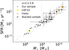 |
Fig. A.1. SFR and M⋆ for the full sample (black circles), the stacked sample (gray squares with error bars), the three sources in udf-10 (yellow circles), and the individual Si II* halos (red crosses), compared to those of galaxies z = 2.1–3.9 in the DR2 catalog (gray dots). Due to the large 1σ uncertainties in SFR and M⋆ (Bacon et al. 2023), error bars are shown only for the stacked sample" for clarity and conciseness. The full sample lies along the relation for the galaxies at z = 2.1–3.9 in the same catalog, which suggests that our sample is not biased toward starburst galaxies. |
Next, we examine potential differences between the two fields. Sources in mxdf are widely distributed and include low-mass sources with faint magnitudes (see also Fig. 2). Among the three sources in udf-10 (yellow circles), two are located at the massive end of the sequence in Fig. A.1, while the remaining one has a low stellar mass. As expected from the depth of the MUSE data, the fractions of low-mass sources with low SFRs and faint magnitudes in mxdf are higher than those in udf-10, regardless of thresholds. However, because of the small sample size in udf-10 (N = 3), our main results are unlikely to be significantly affected by the depth of udf-10. Studying the fractions and extents of halos is beyond the scope of this paper, which requires a larger sample and careful assessment of the inhomogeneous data set (see Appendix B.1 for the examination of the SB limits for our sources). In Appendix B.2, we discuss potential differences in SFR and M⋆ for individually detected halos and nonhalos.
Overview of the sample
Appendix B: Potential effects of different depths and sample properties
B.1. Potential effects of different depths of the MUSE data for our sample
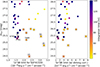 |
Fig. B.1. Distributions of 1σ SB limits of Si II* λ1533 and apparent UV magnitudes for our sample. The left panel shows 1σ SB limits on a 1-arcsec2 scale for the Si II* λ1533 NBs, while the right panel shows 1σ SB limits multiplied by (1+z)4/(1+z1141)4 to account for the effect of cosmic dimming in a relative manner. The color bar indicates the integration time. The stacked subsample is enclosed by gray squares, and the individually detected Si II* halos are indicated by red crosses (see Sect. 3.2 ). The MUSE IDs for the seven objects with mUV ≲ 25.5, which are brighter than the faintest individually detected halo (ID=51) are shown in the left panel. Detection rates of halos are expected to depend on the SB limits of the data set, but the panels do not show any clear trend, likely due to the limited sample size and different sample properties. |
As mentioned in Sect. 3.2, we have five individual detections of Si II* λ1533 halos. Three of these sources are located in udf-10 with the integration time of 31 hours, while the remaining two are in mxdf with the integration times ranging from 32 hours to 141 hours (see Fig. 2 and Table A.1). The SB limits of the NBs used in this work depend not only on the integration time but also on the observed wavelength (i.e., redshifts of the sample). The effect of cosmic dimming is also significant and cannot be ignored. Therefore, we discuss potential effects of 1σ SB limits and cosmic dimmings on the detectability. If the origin of Si II* emission is continuum pumping as suggested in this paper, bright UV magnitudes are necessary to produce bright Si II* emission (in terms of observed, apparent magnitudes). We examine distributions of 1σ SB limits on a 1-arcsec2 scale for the Si II* λ1533 NBs and apparent UV magnitudes for our sources in Fig. B.1 (with integration times indicated by the color bar). We estimate the 1σ SB limits for each object from a sensitivity table for mxdf and udf-10 in Bacon et al. (2023), considering the narrow-band widths and integration times (see the left panel). The right panel shows the 1σ SB limits multiplied by (1+z)4/(1+z1141)4 to account for the effect of cosmic dimming in a relative manner, where z1141 is the systemic redshift of our best-case object, ID=1141 (zsys = 2.34). For instance, the actual depth of the Si II* NB of ID=50 is 3 × 10⁻¹⁹ erg s−1 cm−2 arcsec−2 (1σ, left panel). Additionally, because of the cosmic dimming effect, the SB level of ID=50 at zsys = 3.32 becomes 3.3 times fainter compared to the case where it was located at zsys = 2.34. In relative terms, it corresponds to the 1σ SB limit of 9 × 10⁻¹⁹ erg s−1 cm−2 arcsec−2 (right panel). Considering these two effects, the corresponding noise level of ID = 50 is seven times higher than that of ID = 1141, which is presented relatively as a correction in the right panel. The noise levels shown in the right panel are less dependent on the integration time (different fields) than those in the left panel. This exercise indicates that the depth of the data indeed depends on the redshifts as well as integration times.
As shown in Fig. B.1, we cannot conclude any dependence of Si II* halo detections (red crosses) and nondetections on the SB limits as well as integration times. Even when focusing on bright objects with mUV ≲ 25.5, which are brighter than the faintest individually detected halo (ID=51), and whose IDs are shown in the left panel, no clear trends are observed. The SB limits of two nonhalos (ID=6700 at zsys = 2.99 and ID=7600 at zsys = 2.57 in mxdf) are deeper than that of ID=50 at zsys = 3.32 in udf-10. We note that the Si II* λ1533 of one of the UV brightest objects, ID=8048, drops in the AO gap in the MXDF and is not included in this plot. A larger sample is needed to rigorously test the detectability depending on the depth of the data set. In the next section we discuss the differences in sample properties.
B.2. Potential differences in properties between Si II* halo sources and nonhalo sources
We check potential differences in SFR and M⋆ between Si II*-halo sources (red crosses) and nonhalo sources (black circles) shown in Fig. A.1, though their uncertainties are large. We find that halos tend to have high SFR and M⋆, which is expected from the trend with UV magnitudes (Figs. 2 and B.1). However, not all the sources with high SFR, high M⋆, or high MUV (mUV) show a clear Si II* halo. Among them, apparent UV magnitudes (i.e., MUV and redshifts) would be most strongly related to the detection of the halos. It is indeed consistent with the continuum pumping as the mechanism of Si II* emission. We need a larger sample to investigate the dependence of the detectability and existence of halos on data qualities and sample properties.
All Tables
All Figures
|
Fig. 1. Energy levels of Si+ ions and different channels of excitation and de-excitation from the ground-state or the fine-structure level (fluorescence) for Si II* λ1265, 1309, 1533 lines in panels (a) to (c), respectively. The probabilities (P) of related transitions and their wavelengths are also shown. The ionization energies of these LIS lines are close to that of H I. The Si II* lines can be regarded as an escape channel of photons from Si II resonant scattering. |
| In the text | |
|
Fig. 2. Redshift distribution of our sample. (Top) Redshift ranges covered for the Si II* λ1265, 1309, and 1533 lines. Dark blue and yellow indicate mxdf and udf-10, respectively. The gaps between the dark blue bars are the AO gap (see Sect. 2.1). (Middle) MUV and zsys distribution of our sample with MUSE IDs. The color bar at the right indicates the integration time. The stacked subsample is enclosed by gray squares. The MUV corresponding to mUV = 26.0 (magnitude cut for the stacking sample) at each redshift is shown by the black dashed line. The individually detected Si II* halos are indicated by red crosses (see Sect. 3.2 ). (Bottom) 1σ SB limits for Si II* λ1533 in mxdf (dark blue) and udf-10 (yellow), which are converted from the median surface brightness limits on the sensitivity table in Bacon et al. (2023) using the narrow band widths for Si II* λ1533 for given redshifts (see Sect. 3.1). The Si II* halos tend to have bright MUV. |
| In the text | |
|
Fig. 3. Images and spectra for Si II* halos. (From left to right) The HST image, MUSE UV-continuum BB image, MUSE Si II* NB image, SB profile, and Si II* spectrum for the five sources with Si II* halo detections. Each row (except the fifth) shows the Si II* λ1533 line for a different object. The fifth row shows a coadded result of three Si II* lines for MID = 50 at z = 3.32, whose three Si II* lines (Si II* λ1265, Si II* λ1309, and Si II* λ1533) are covered with MUSE. The image size is five arcsec. The gray shades indicate masked spaxels. For presentation purposes, NB images are smoothed with a Gaussian kernel with σ = 1.5 spaxel. The white contours correspond to 1 × 10⁻¹⁹ erg s−1 cm−2 arcsec−2 (the typical 3σ SB limit in MXDF for an unresolved emission; Bacon et al. 2023). The cyan crosses indicate the HST center. The SB profiles of the UV continuum (black lines) are normalized at the innermost radius (R = |
| In the text | |
|
Fig. 4. Stacking results. From left to right, we show the mean-stacked UV continuum image, the mean-stacked Si II* emission image (5 arcsec each), the mean surface brightness profiles, the median-stacked UV continuum image, and the median-stacked Si II* emission image. The top and bottom panels represent stacking results of the Si II* λ1533 line (N = 13) and those of all Si II* lines (22 images for 14 sources), respectively. The cyan crosses indicate the HST center. The white contours correspond to 5 × 10⁻²⁰ erg s−1 cm−2 arcsec−2, which is also shown by black dotted lines on the SB profiles. The SB profiles of the mean-stacked Si II* and UV continuum are indicated by the blue and black lines, respectively, while the median-stacked Si II* and UV continuum are shown by the blue and the black crosses, respectively. The blue and gray shades represent 1σ uncertainties of the SB for Si II* emission and UV continuum, respectively. Following Fig. 3, the SB profiles for the continuum are normalized at the innermost radius (R = |
| In the text | |
|
Fig. 5. Curve of growth (CoG) for Si II* flux and EW for MID = 1141. Left: Normalized fluxes within radius R as a function of R measured from the Si II* NB image (blue line) and the UV continuum BB image (black line). The blue shade indicates 1σ uncertainties for the Si II* flux. The vertical magenta lines show R = |
| In the text | |
|
Fig. 6. Galaxy-scale and CGM-scale spectra for MID = 1141. Left: Spectrum extracted from the original minicube (black line) with a |
| In the text | |
|
Fig. 7. Stacked SB profiles of our observations and of zoom-in simulations from Mauerhofer et al. (2021). Left: Comparison of stacked SB profiles. The blue and black solid lines show the observed mean-stacked SB profiles of Si II* λ1533 and the continuum, respectively. The blue shade indicates 1σ uncertainties for Si II* λ1533. The observed continuum is normalized at R = 0 to the peak of the observed Si II* λ1533. The green and gray dotted lines (shades) show the mean-stacked SB profiles of Si II* λ1533 and the continuum, respectively, for the simulations after PSF and LSF convolution (their 1σ uncertainties, which correspond to the 15.87 to 84.13 percentiles of SB profiles for individual mocks). They are normalized at R = 0 to the peak of the observed Si II* profile. Right: Stacked SB profiles for simulations. The green and gray dotted (solid) lines show the mean-stacked SB profiles of Si II* λ1533 and continuum, respectively, with (without) PSF and LSF convolution. The green and gray crosses show the median-stacked SB profiles of Si II* λ1533 and the continuum, respectively, with PSF and LSF convolution. They are scaled by the same factor as used in the left panel. The left panel shows that the observed stacked SB profiles can be reproduced within the 1σ uncertainties by the simulations, which account for continuum pumping. |
| In the text | |
|
Fig. 8. EW CoG and spectra of the simulations with continuum pumping. Left: Median cumulative EW in rest-frame as a function or R. The blue and red solid lines (shades) indicate the EW of Si II* λ1533 emission and Si IIλ1527 absorption lines (their 1σ uncertainties) with MUSE PSF convolution, respectively. The cyan and magenta dashed lines (shades) show the intrinsic EW of Si II* λ1533 emission and the Si IIλ1527 absorption lines (their 1σ uncertainties). Middle: Median spectrum extracted from the intrinsic mock cube with a 1.2 kpc aperture (galaxy scale) shown by the black line. The cyan and magenta lines show the wavelength of Si II* λ1533 emission and Si IIλ1527 absorption lines, respectively. Right: Median spectrum extracted from the intrinsic mock cube with a 19 kpc aperture (CGM scale). The EWs of the Si II* λ1533 emission and Si IIλ1527 absorption are consistent on a CGM scale for both intrinsic cubes and PSF-convolved cubes, which are also seen on the mock spectra. |
| In the text | |
|
Fig. A.1. SFR and M⋆ for the full sample (black circles), the stacked sample (gray squares with error bars), the three sources in udf-10 (yellow circles), and the individual Si II* halos (red crosses), compared to those of galaxies z = 2.1–3.9 in the DR2 catalog (gray dots). Due to the large 1σ uncertainties in SFR and M⋆ (Bacon et al. 2023), error bars are shown only for the stacked sample" for clarity and conciseness. The full sample lies along the relation for the galaxies at z = 2.1–3.9 in the same catalog, which suggests that our sample is not biased toward starburst galaxies. |
| In the text | |
|
Fig. B.1. Distributions of 1σ SB limits of Si II* λ1533 and apparent UV magnitudes for our sample. The left panel shows 1σ SB limits on a 1-arcsec2 scale for the Si II* λ1533 NBs, while the right panel shows 1σ SB limits multiplied by (1+z)4/(1+z1141)4 to account for the effect of cosmic dimming in a relative manner. The color bar indicates the integration time. The stacked subsample is enclosed by gray squares, and the individually detected Si II* halos are indicated by red crosses (see Sect. 3.2 ). The MUSE IDs for the seven objects with mUV ≲ 25.5, which are brighter than the faintest individually detected halo (ID=51) are shown in the left panel. Detection rates of halos are expected to depend on the SB limits of the data set, but the panels do not show any clear trend, likely due to the limited sample size and different sample properties. |
| In the text | |
Current usage metrics show cumulative count of Article Views (full-text article views including HTML views, PDF and ePub downloads, according to the available data) and Abstracts Views on Vision4Press platform.
Data correspond to usage on the plateform after 2015. The current usage metrics is available 48-96 hours after online publication and is updated daily on week days.
Initial download of the metrics may take a while.