| Issue |
A&A
Volume 696, April 2025
|
|
|---|---|---|
| Article Number | A95 | |
| Number of page(s) | 20 | |
| Section | Extragalactic astronomy | |
| DOI | https://doi.org/10.1051/0004-6361/202452493 | |
| Published online | 08 April 2025 | |
Connecting the growth of galaxies to the large-scale environment in a massive node of the Cosmic Web at z ∼ 3
1
Dipartimento di Fisica G. Occhialini, Università degli Studi di Milano Bicocca, Piazza della Scienza 3, 20126 Milano, Italy
2
Department of Astronomy, California Institute of Technology, 1200 E. California Boulevard, MC 249-17, Pasadena, CA 91125, USA
3
INAF – Osservatorio Astronomico di Brera, Via Brera 28, I-21021 Milano, Italy
4
INAF – Osservatorio Astronomico di Trieste, Via G. B. Tiepolo 11, I-34143 Trieste, Italy
5
The Carnegie Science Observatories, 813 Santa Barbara Street, Pasadena, California 91101, USA
⋆ Corresponding author; This email address is being protected from spambots. You need JavaScript enabled to view it.
Received:
4
October
2024
Accepted:
5
February
2025
Abstract
A direct link between the large-scale environment and galaxy properties is very well established in the local Universe. However, very little is known about the role of the environment for galaxy growth before the peak of the cosmic star formation history at z > 3 due to the rarity of high-redshift, overdense structures. Using a combination of deep, multiwavelength observations, including MUSE, JWST, Chandra, HST, and ground-based imaging, we detected and studied the properties of a population of star-forming galaxies in the field of a hyperluminous quasar at z ≈ 3.25 associated with the giant Lyα nebula MQN01. We find that this region hosts one of the largest overdensities of galaxies discovered so far at z > 3, with ρ/ρ̄ = 53 ± 17 within 4 × 4 cMpc2 and |Δv|≤1000 km s−1 from the quasar, providing a unique laboratory for studying the link between overdense regions and galaxy properties at high redshift. Even in these rare overdense regions, galaxies form stars at a rate consistent with the main sequence at z ≈ 3, demonstrating that their star formation rate (SFR) is regulated by local properties correlated with their stellar mass rather than by their environment. However, the high-mass end of the stellar mass function is significantly elevated with respect to that of galaxies in the field at log(M⋆/M⊙)≳10.5, suggesting that massive galaxies in overdense regions build up their stellar mass earlier or more efficiently than in average regions of the Universe. Finally, the overdensity of color-selected Lyman break galaxies observed on larger scales, across ≈24 × 24 cMpc2, is found to be aligned toward the structure traced by the spectroscopically confirmed galaxies identified with MUSE in the inner 4 × 4 cMpc2, suggesting that this highly overdense region could extend further, up to a few tens of comoving megaparsecs.
Key words: galaxies: evolution / galaxies: high-redshift / galaxies: star formation / large-scale structure of Universe
© The Authors 2025
 Open Access article, published by EDP Sciences, under the terms of the Creative Commons Attribution License (https://creativecommons.org/licenses/by/4.0), which permits unrestricted use, distribution, and reproduction in any medium, provided the original work is properly cited.
This article is published in open access under the Subscribe to Open model. This email address is being protected from spambots. You need JavaScript enabled to view it. to support open access publication.
1. Introduction
According to the current cosmological model, most of the inter-galactic gas is distributed in a network of filaments and sheets, called the Cosmic Web, formed through gravitational collapse of the initial density fluctuations (Bond et al. 1996). Structures form in the densest part of the Cosmic Web and grow hierarchically, merging into the massive virialized groups and clusters we observe in today’s Universe at the intersection of filaments (see e.g., de Lapparent et al. 1986; Geller & Huchra 1989; Alpaslan et al. 2014; Libeskind et al. 2018). This large-scale environment is thought to play a key role in regulating how the embedded galaxies form and evolve across cosmic time. In fact, galaxies found in virialized clusters at z ≲ 1 are more massive and form stars at a lower rate than the galaxies living in the field (see e.g., Baldry et al. 2006; Bamford et al. 2009; Peng et al. 2010; Calvi et al. 2013; Tomczak et al. 2017, 2019; Lemaux et al. 2019; Old et al. 2020; Chartab et al. 2020; van der Burg et al. 2020; McNab et al. 2021). Thus, it is implied that galaxies inhabiting extremely overdense regions assemble their mass either more rapidly or at earlier times than those in the field and undergo intense episodes of star formation (see e.g., Thomas et al. 2005; Raichoor et al. 2011; Gu et al. 2018). Therefore, the z ≳ 2 progenitors of present-day clusters, often referred to as protoclusters (Sunyaev & Zeldovich 1972; Cen & Ostriker 2000; Overzier 2016; Alberts & Noble 2022), are an ideal laboratory within which we can study the fundamental link between galaxies and their large-scale environment.
Overdensities of Lyα and Hα emitters, Lyman break galaxies (LBGs) or dusty star-forming galaxies, are commonly used as a tracer for candidate cluster progenitors (see e.g., Steidel et al. 1998, 2000; Kurk et al. 2000, 2004; Hayashino et al. 2004; Chapman et al. 2009; Tanaka et al. 2011; Lee et al. 2014; Casey et al. 2015; Oteo et al. 2018; Shi et al. 2019a,b), although their spatial distribution does not necessarily follow fully virialized structures (Lovell et al. 2018; Toshikawa et al. 2020), unlike z ≈ 0 clusters. Indeed, at z ≳ 2, Chiang et al. (2013) predicted protoclusters to extend over ≈10 − 20 cMpc, while some well-studied structures show multiple peaks in their galaxies’ overdensity and extend on even much larger scales (see e.g., Steidel et al. 1998; Pentericci et al. 2000; Cucciati et al. 2018). In similar z ≳ 2 overdense environments, galaxies are found to be sites of higher star formation activity and their stellar mass function shows an excess at the high-mass end compared to the field (see e.g., Kodama et al. 2007; Koyama et al. 2013a,b; Shimakawa et al. 2018a,b; Greenslade et al. 2018; Miller et al. 2018; Ito et al. 2020; Lemaux et al. 2022; Taamoli et al. 2024; Toshikawa et al. 2024) as well as enhanced active galactic nuclei (AGN) activity (e.g., Lehmer et al. 2009; Tozzi et al. 2022; Gatica et al. 2024). A high rate of mergers (Alonso et al. 2012; Mei et al. 2023), efficient gas accretion (e.g., D’Amato et al. 2020), and interactions with a proto-intracluster medium (Di Mascolo et al. 2023) are expected to play a key role in regulating galaxy growth and activity in these high-redshift overdensities. Although star-forming galaxies are observed to be the dominant population in clusters’ progenitors (Kuiper et al. 2010; Spitler et al. 2012; Contini et al. 2016), the detections of quiescent galaxies have been reported in some structures (Kodama et al. 2007; Kubo et al. 2013; Shi et al. 2019b). These observations suggest that protoclusters could be ideal environments to study the onset of environmental quenching and the processes driving the suppression of the star formation activity observed in z ≈ 0 clusters galaxies. Theoretical works (e.g., Muldrew et al. 2015; Chiang et al. 2017; Lovell et al. 2018) are consistent with these observational results, and both support a picture in which galaxies in protoclusters have assembled their masses and rapidly grown at earlier times than those in the field.
Complementary to blind searches, overdense structures of the inter-galactic medium (IGM) itself (mapped via three dimensional Lyα tomography, see e.g., Lee et al. 2018; Newman et al. 2020, 2022), as well as the surroundings of highly biased objects, such as high-redshift radio galaxies (HzRGs; e.g., Roettgering et al. 1994; Pentericci et al. 2000; Hayashi et al. 2012; Hatch et al. 2014; Rigby et al. 2014; Orsi et al. 2016; Pérez-Martínez et al. 2023), hot dust-obscured galaxies (Hot DOGs; Jones et al. 2014; Assef et al. 2015; Penney et al. 2019; Luo et al. 2022; Ginolfi et al. 2022; Zewdie et al. 2023), and luminous quasars (QSOs; e.g., Kashikawa et al. 2007; Venemans et al. 2007; Overzier et al. 2008; Priddey et al. 2008; Kim et al. 2009; Utsumi et al. 2010; Bañados et al. 2013; Husband et al. 2013; Adams et al. 2015; Mignoli et al. 2020; Kashino et al. 2023) have been typically explored as signposts of galaxy overdensities. In particular, high-redshift QSOs are among the brightest objects in the z ≳ 2 Universe and are thus expected to trace overdense structures. Indeed, a hyperluminous QSO at z ≈ 2.84 was found at the center of a large overdensity of LBGs (Steidel et al. 2011), Lyα emitters (Kikuta et al. 2019), and submillimeter galaxies (Lacaille et al. 2019; Wang et al. 2024a), tracing a large-scale structure extending across ≈100 cMpc. Garcia-Vergara (2021) explored the galaxy clustering around z ≈ 4 QSOs and found a large overdensity of different galaxy populations, that is, CO(4–3) line emitters and Lyα emitting galaxies. On the other hand, Falder et al. (2011), Trainor & Steidel (2012), Adams et al. (2015), and Hennawi et al. (2015) reported the detection of galaxy overdensities in the environment of luminous QSOs in only ≈10% of the cases.
Despite the increasing number of z ≳ 2 galaxy overdensities and candidate protoclusters discovered in the literature, the heterogeneity of the tracers and the methods adopted to identify the galaxies in their surroundings makes it challenging to draw a unified picture and to consistently trace the assembly and the evolution of the overdense structures down to present-day clusters. Comparing the galaxy environment around radio-loud AGNs from the Clusters Around Radio-Loud AGNs (CARLA; Wylezalek et al. 2013) program and radio-quiet QSOs with similar masses and redshifts, Hatch et al. (2014) found that the choice of the biased tracer itself has an effect on the large-scale galaxy environment identified in its surroundings. Indeed, on average, radio-loud AGNs are observed to be surrounded by larger overdensities and to trace larger structures than radio-quiet QSOs. Additionally, differences among overdensities of galaxies selected with a similar criterion around the same biased tracer may arise as a consequence of these structures being in a different evolutionary stage, as shown by, e.g., Shimakawa et al. (2018b).
We present in this work a multiwavelength survey of the large-scale galaxy environment around the z ≈ 3.25 QSO CTS G18.01, which has been preselected for being surrounded by extended and filamentary-shaped Lyα emission from the cosmic gas (named MQN01), as discovered by Borisova et al. (2016) and as confirmed later by deeper observations covering a wider area (Cantalupo et al., in prep.). In particular, we targeted the field with a mosaic of observations taken with the Multi Unit Spectroscopic Explorer (MUSE; Bacon et al. 2010) at the Very Large Telescope (VLT), the FOcal Reducer and low dispersion Spectrograph 2 (FORS2; Appenzeller et al. 1998) and the High Acuity Wide field K-band Imager (HAWK-I; Pirard et al. 2004; Casali et al. 2006; Kissler-Patig et al. 2008; Siebenmorgen et al. 2011) at the VLT. The combination of these datasets aims at selecting star forming galaxies at the redshift of the QSO across 24 × 24 cMpc2 and provides spectroscopic confirmation within an area of 4 × 4 cMpc2 that is covered by MUSE. Additional ALMA, HST/ACS, JWST/NIRCam and Chandra observation are used to derive star formation rates and stellar masses by modeling the galaxies’ spectral energy distribution (SED) and to explore this peculiar environment in the context of galaxy formation and evolution. The goal of this work is thus to exploit this rich multiwavelength dataset to explore an overdense region at z ≈ 3 (Pensabene et al. 2024) and unveil the roles of both the local and large-scale environment on the stellar mass assembly and star formation activity of the galaxies populating this unique field.
We describe the data in Section 2 and present in Section 3 the samples of galaxies identified around the target QSO. In Sections 4.1–4.3 we investigate the overdensity of star-forming galaxies within 4 × 4 cMpc2 around the QSO and explore their properties, compared to galaxies in the field, in Sections 4.4–4.6. We then explore the overdensity of LBGs across 24 × 24 cMpc2 in Section 4.7. Finally, we discuss this structure in the context of galaxy formation and evolution in Section 5. Throughout, unless otherwise noted, we quote magnitudes in the AB system, distances in physical units, and adopt Planck 2015 cosmology (Ωm = 0.307, H0 = 67.7 km s−1 Mpc−1; Planck Collaboration I 2016).
2. Observations and data reduction
2.1. MUSE observations
The main dataset consists of a mosaic of four VLT/MUSE pointings around the QSO CTS G18.01. The observations are part of the MUSE Guaranteed Time Observations (GTO) programme ID 0102.A-0448(A), PI S. Cantalupo. They were all conducted in October 2018 in visitor mode with an integration time of, on average1, ≈10 hours per pointing using MUSE with AO in Wide-Field mode. Data were taken on clear nights, at airmass ≤2.8, angular distance from the moon ≥30 deg, lunar illumination ≤20% and requiring an image quality better than FWHM ≤ 0.8 arcsec. The different frames of each pointing were observed with a relative orientation of 90 degrees and small dithers (≲1 arcsec) to mitigate the differences in the performance of the 24 IFUs (see e.g., Borisova et al. 2016; Marino et al. 2018). Each of the pointings covers 1 × 1 arcmin2, resulting in a final mosaic with a Field-of-View (FoV) of ≈2 × 2 arcmin2 which corresponds to 4 × 4 cMpc2 at the redshift of the central QSO, z ≈ 3.25.
The raw data were initially reduced with the ESO MUSE pipeline (Weilbacher et al. 2014, version 2.8.1). The SCIBASIC routine of the ESO MUSE pipeline was used to subtract bias, apply flat fielding, perform twilight and illumination corrections, calibrate the wavelengths and the line spread function using arcs, and reduce the sky flats. The same calibrations are applied to the field targeting the standard star, which is then used to calibrate the flux. The known astrometric offsets (Bacon et al. 2015) are corrected by registering the datacubes using the point sources identified in each collapsed individual frame. Once aligned, all individual frames are combined in a final datacube by using a 3D drizzling interpolation process. The final stacked datacubes produced by the ESO pipeline are known (see e.g., Borisova et al. 2016; Bacon et al. 2017; Marino et al. 2018; Cantalupo et al. 2019) to be affected by imperfections in the flat fielding process and instabilities of the detector. To correct for these effects and improve the quality of the datacubes, we post-process the final products using the CUBEXTRACTOR (CUBEX hereafter, see, de Beer et al. 2023 and Cantalupo et al., in prep.) package, version 1.8, and its subroutines (see Figure 1 in Lofthouse et al. 2020 for an example of the post-processing results compared to the science products reduced by the ESO pipeline). In detail, CUBEF IX applies the flat-fielding correction by using the observed sky to self-calibrate the exposures. This process is applied iteratively after masking the continuum-detected sources to avoid contamination. The result is an optimal realignment of the relative illumination between the stacks and slices of each IFU, which are not completely corrected by the daily flats. CUBESHARP performs flux-conserving sky subtraction by including empirical corrections of the line spread function. By means of the CUBECOMBINE tool, we then combined the individual exposures into a single datacube. This cube is then used to mask continuum sources detected in the collapsed white-light image to optimize a second iteration of CUBEF IX and CUBESHARP. Finally, CUBECOMBINE is used to produce the final and fully reduced datacube.
2.2. FORS2 and HAWK-I mosaics
We followed up the MUSE observations with a joint VLT/FORS2 and VLT/HAWK-I programme (ID 110.23ZX, PI S. Cantalupo). The FORS2 mosaic is designed to cover an area of ≈24 × 24 cMpc2, which corresponds to a FoV that is ≈6 × 6 larger than the MUSE one and to overlap in the same area covered by MUSE. The observations were executed during ESO Cycle 110-111 in both visitor and service mode, as detailed below, and consist of imaging in three different filters: UHigh (7 h on source, λeff = 361 nm), BHigh (5 h on source, λeff = 437 nm) and RSpecial (45 minutes on source, λeff = 655 nm). The U-band data were taken in visitor mode during two half-nights in October 2022 (Run ID 110.23ZX.001) with the blue-sensitive E2V FORS2 CCD. The B-band and R-band observations were taken in service mode with the MIT CCD. The observations in all three filters were executed with the default CCD read-out mode for imaging, 2 × 2 binning, and low gain. Our observational constraints include clear nights, airmass ≤1.5, ≤20% lunar illumination, and a seeing better than 0.8 arcsec FWHM. We observed each mosaic position twice and applied small dithers between the individual frames in each individual OB to improve contamination removal, background subtraction and to cover the gap between the two chips. To reduce the data, we used the ESO pipeline recipes for FORS2 (Izzo et al. 2010, version 5.6.2) to apply standard bias, flat, and flux calibrations2. The 2D background was locally modeled and subtracted using the python package PHOTUTILS (Bradley et al. 2023, version 1.9.0). Finally, we aligned the astrometry of each individual frame with stars from Gaia DR3 catalog (Gaia Collaboration 2016, 2023) by using the SCAMP package (Bertin 2006, version 1.20). The reduced and registered frames are sigma-clipped and combined into a large-scale mosaic using SWARP (Bertin 2010, version 2.21).
To characterize the depth of the final mosaics, we measured the 3σ limiting magnitude of each image (see Table 1) within apertures of radius r = 4 pixels ≈ 1 arcsec, corresponding to twice the maximum value of the PSF, and placed in 5000 random positions in blank regions, with all sources masked to avoid contamination. To estimate the image quality of the science products, we used the software PSFEX (Bertin et al. 2011) that extracts a sample of unsaturated stars to measure the Point Spread Function (PSF) across the entire FoV accounting for spatial variations. We report the mean value across the FoV in Table 1, which will also be used to perform accurate photometry later in the analysis: the variation between the minimum and maximum PSF across the FoV is ≲10% for all images.
Depth and PSF FWHM of the VLT/FORS2 imaging observations.
As a final step, we performed injection and recovery experiments to estimate the completeness of the science mosaics. We first created background-only versions of the images by replacing each pixel belonging to known sources, as identified by SEXTRACTOR (Bertin & Arnouts 1996, version 2.24.2) using the same parameters listed in Section 3.1, with a value randomly extracted from a normal distribution centered on the median value of the background. To create artificial sources, we convolved point sources with the PSF and randomly injected 1500 mocks for each Δm = 0.025 mag bin of magnitude, from m = 24 mag to m = 31 mag, in the background-only mosaics. The number of mocks is carefully chosen to avoid overlap and deblending issues. We then run SEXTRACTOR and measured the fraction of sources we can recover as a function of magnitude. We computed the results (see Figure 1 and Table 1) for the full mosaic, distinguishing three different regions (the deepest one is designed to overlap with the MUSE FoV in the center of the mosaic) depending on the number of exposures.
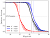 |
Fig. 1. Completeness estimated for the VLT/FORS2 images in the U (blue), B (black), and R band (red). The solid line is the result across the entire FoV, while the shaded regions reproduce the variation from the shallower to the deepest regions of each mosaic. The vertical dotted lines mark the magnitudes corresponding to the 50% completeness limit (black horizontal line). |
The survey strategy described above for the FORS2 observations was employed to image the same area of ≈24 × 24 cMpc2 around the target QSO with VLT/HAWK-I. We observed the field with a set of three filters: CH4 (1 h on source, λeff = 1.575 μm), H (2 h on source, λeff = 1.620 μm) and Ks (2 h on source, λeff = 2.146 μm). The observations were executed in October-December 2022 with AO requiring the same constraints listed for FORS2. The raw data were bias subtracted, flat fielded and flux calibrated by using the ESO Pipeline recipes for HAWK-I imaging (version 2.4.13) implemented in ESOREX (ESO CPL Development Team 2015, version 3.13.6). The 2MASS (Skrutskie et al. 2006) catalog is used to measure the flux zero-point. After subtracting the background, we used the HAWKI_SCIENCE_POSTPROCESS recipe in the ESO Pipeline to combine the exposures into the final science mosaic. As a final step, we registered the astrometry of the final mosaic to Gaia by using the DRIZZLEPAC package3 (Gonzaga et al. 2012; Hoffmann et al. 2021). We report the 3σ magnitude limit and the PSF FWHM in Table 2.
Depth and PSF FWHM of the HST/ACS, VLT/HAWK-I, and JWST/NIRCam observations.
2.3. Multiwavelength photometry and ancillary data
This field has also been targeted by a multiwavelength campaign spanning from the X-Ray to millimeter wavelengths (see the left panel in Figure 2), which enables us to perform a complete census of the different populations of sources in the environment of the central QSO, including AGN and dusty star-forming galaxies, which may be elusive in optical observations. Travascio et al. (2025) collected 600ks of broadband (0.5–7.0 KeV) observations with the Advanced CCD Imaging Spectrometer (ACIS) mounted onboard the Chandra spacecraft (Weisskopf et al. 2000) during Cycle 23 (PI: S. Cantalupo). The final FoV extends above the 24 × 24 cMpc2 observed by FORS2 and HAWK-I and provides ≈1 arcsec resolution imaging and moderate resolution spectroscopy. We also observed the field with the Hubble Space Telescope (HST) for a total of 22 orbits in Cycle 30 (PID: 17065, PI: S. Cantalupo) and used the HST/ACS (Advanced Camera for Survey, Ford et al. 1998) instrument to image a ≈3.4 × 3.4 arcmin2 FoV around the central QSO with the filters ACS F625W (25 397 s) and ACS F814W (30 238 s). We complemented our multiwavelength dataset with the James Webb Space Telescope (JWST, Rigby et al. 2023) pre-imaging observations associated with the GO Cycle 1 programme ID 1835 (Cantalupo et al. 2021, PI S. Cantalupo). With an on-source exposure time of ≈2 × 27 minutes, we pointed JWST/NIRCam to image a 2 × 5 arcmin2 FoV with the extra-wide filters F150W2 (in the short wavelength channel, 0.6 − 2.3 μm) and F322W2 (in the long wavelength channel, 2.4 − 5.0 μm). Details on the data reduction are reported in Wang et al. (2024b). In Table 2 we report the depth, in terms of 3σ magnitude limit, and the PSF FWHM of all these observations. Finally, Pensabene et al. (2024) targeted the field with a Cycle 8 ALMA programme (ID 2021.1.00793.S, PI S. Cantalupo) surveying the 4 × 4 cMpc2 MUSE FoV with Band 3 and Band 6 mosaics to detect dusty star forming galaxies via their 1.2 mm continuum emission or CO(4–3) emission lines. The data and the reduction steps are detailed in Pensabene et al. (2024).
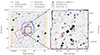 |
Fig. 2. Visualization of the multiwavelength data explored in this work. Left panel: FORS2/R-band image with overlaid the footprint of the MUSE (purple), FORS2 and HAWK-I (orange), HST/ACS F625W (blue), HST/ACS F814W (light-blue), JWST/NIRCam (red) and ALMA/Band3 and Band6 (green) observations. Right panel: the zoom-in shows the MUSE White-Light image in the background with highlighted the MQN01 high-confidence sample of galaxies found in the MUSE FoV within a line-of-sight separation |Δv|≤1000 km s−1 around the QSO (blue squares), the cross-matched CO(4–3) line-emitters found by ALMA (green diamonds, see Pensabene et al. 2024) and X-Ray sources detected by Chandra (red circles, see Travascio et al. 2025). The target QSO is marked by a gold star. |
3. Data analysis
We describe in this section the methods we adopted to search for galaxies around the target QSO. The rest-frame UV color selections used to identify LBGs in the FORS2 images are detailed in Section 3.1 and Appendix A. The sample of continuum-selected galaxies identified in the MUSE mosaic, as well as their spectroscopic redshift measurements, is described in Section 3.2.
3.1. Photometric selection of Lyman break galaxies
To identify the LBGs at z ≈ 3 − 3.5 across the FORS2 FoV, we calibrated a selection based on U − B and B − R colors (see e.g., Bielby et al. 2011). We carefully choose those photometric bands to avoid any possible contamination due to the presence of bright Lyα emission which may be arising from the recombination of the ionizing radiation emitted by the central QSO, rather than from the galaxies’ activity. To calibrate the selection region, we used BPASS SPS models (Stanway & Eldridge 2018, v2.2-100bin-t8.0-Z001) with a Salpeter IMF (Salpeter 1955) up to a stellar mass limit of M⋆ = 100 M⊙, binary evolution and stellar metallicity Z⋆ = 0.001 (corresponding to Z⋆ ≈ 0.07 Z⊙ with solar abundances from Asplund et al. 2009). We assumed a constant star formation history and stellar age of t = 100 Myr, chosen to be consistent with the median age of the stellar population of the galaxies identified in MUSE (see Section 3.4 and also Steidel et al. 2018 for a similar approach). We also considered discrete values of reddening: E(B − V) = 0, 0.05, 0.10, 0.15, 0.20, which are typical values for LBGs at z ≈ 3 (see e.g., Shapley et al. 2003). The models are then post-processed to account for the attenuation due to the absorption from the inter-galactic medium. We thus generated 500 IGM realizations randomly extracted from 1000 sightlines from Steidel et al. (2018) and produced by inserting along each line-of-sight intervening H I absorption-line systems, based on their column density distribution function reported in Rudie et al. (2013), to reproduce the stochastic nature of the IGM absorption. Finally, the color criterion requires the following:
-

-
U−B > 1.00
-
B−R < 1.74 ×(U−B)−1.24
-
0.31 < B−R < 2.20.
The first condition corresponds to requiring that the source is not detected in U-band above 3σBKG, where σBKG is the RMS of the background measured within the same aperture used for colors, and is added to avoid contamination from sources at lower redshift and stars (see an application of this same criterion to select U-dropout galaxies at z ≈ 3 in van der Burg et al. 2010).
We choose the R-band as the detection image and run SEXTRACTOR with the following parameters: (i) THRESHOLD = 1.5 weighted on the mosaic exposure map to ensure a uniform threshold throughout the FoV; (ii) MINAREA = 5 pixels, corresponding to ≈1.3 arcsec2; (iii) default deblending parameters. The image is also filtered with a 3 × 3 Gaussian kernel to optimize the detection of faint objects. Colors are measured within a fixed circular aperture of d = 5 pixels ≈ 1.26 arcsec, although we found that the results do not depend on the radius of the aperture by varying this within the range 0.5 − 2.0 arcsec. The radius is then rescaled for the variations of the PSF between the different images, as listed in Table 1. The results are reported in Figure 3. All candidates have been visually inspected to remove the objects that lie partially outside the edge of the FoV, the photometry of which cannot be performed on the full size of the source. As a result, we identified 535 z ≈ 3.0 − 3.5 LBGs across 24 × 24 cMpc2. The quality of the color selections is tested by cross-matching the catalog of LBG candidates with the spectroscopic sample of galaxies identified in MUSE (Section 3.2), as reported in Table 3.
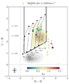 |
Fig. 3. UBR color selection of LBGs. The selection region (delimited by solid black lines) is calibrated based on the redshift tracks of typical LBG templates (dashed lines). The orange density contours show the LBGs candidates at z ≈ 3.0 − 3.5 that are selected by our criterion. The sources with spectroscopic redshift from MUSE and found within |Δv|≤1000 km s−1 from the central QSO are shown as stars and are color-coded by their visual extinction, Av, estimated by fitting their SEDs (see Section 3.4). The gray density contours mark all the R-band detection within the FORS2 FoV. Typical errors on the colors are shown in the lower-left corner. |
Report of UBR and UGR color selections calibrated to identify 3.0 < z < 3.5 LBGs around the central QSO.
3.2. MUSE spectroscopic sample of galaxies
By leveraging the deep MUSE observations, we searched (i) for a spectroscopic confirmation of the color-selected LBGs; (ii) additional continuum-selected sources in proximity to the central QSO that are not detected in the shallower FORS2/R-band nor color-selected as LBGs. To this end, we run SEXTRACTOR in the MUSE white-light image, obtained by collapsing the datacube along the wavelength direction, with the parameters: (i) THRESHOLD = 2.5 rescaled by the RMS of the background to guarantee a uniform threshold across the FoV; (ii) MINAREA = 6 pixels, corresponding to ≈1.2 arcsec2; (iii) minimum deblending parameter DEBLEND_MINCONT = 0.0001. The spectra are extracted within an aperture r = 2.5 × RKron to collect the total flux of the sources. We assign a spectroscopic redshift to the continuum-detected sources using M. Fossati fork4 of MARZ tool (Hinton et al. 2016), which includes additional high-resolution templates suitable for high-redshift galaxies. We attribute confidence scores to the redshift measurements following the method illustrated in Bielby et al. (2019). Figure 4 illustrates examples of sources with high and low confidence levels in their spectroscopic redshift measurements.
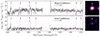 |
Fig. 4. Examples of source classification based on the quality of spectroscopic redshift constraints in MUSE. Left panels: spectra (black) and errors (violet) extracted from MUSE datacubes up to the rest-frame wavelength of the C IV transition (corresponding to observed 6580 Å at z = 3.25), with major spectral features highlighted by vertical dotted lines, as discussed in Section 2.1. When these features are clearly visible, the source is assigned a high-confidence redshift (upper panel). In contrast, when only the Lyα emission line is detected, the redshift measurement is considered low confidence (lower panel). Right panels: 2″ × 2″ cutouts of the MUSE white-light image used for source detection, with the sources indicated by white arrows. |
We are able to assign a high-confidence spectroscopic redshift to ≈38% of the sources. We attribute low confidence to all the sources that exhibit bright Lyα emission at z ≈ zQSO on top of a low signal-to-noise continuum and in the absence of other spectral features. This choice is motivated by the presence of the bright target QSO, which prevents us from ruling out whether the Lyα emission is powered by a z ≈ zQSO galaxy or arises from recombination emission of the QSO radiation on top of a featureless continuum emitted by a foreground or background object. We thus require at least two of the following stellar and interstellar absorption or nebular emission lines to be clearly recognizable in the rest-frame UV spectra: Lyα 1216 Å, N V λ1240 Å, Si II λ1260 Å, O I+Si II λ1303 Å, C II λ1334 Å, Si II λ1526 Å, C IV λλ1548,1550 Å, Fe II λ1608 Å, He II λ1640 Å, Al II λλλ1670, 1854,1862 Å, C III λλ1906, 1908 Å.
With this method, we identify 21 galaxies with high-confidence spectroscopic redshifts lying within a line-of-sight separation |Δv|≤1000 km s−1 from the central QSO (right panel in Figure 2). To prove that our selection of galaxies associated with the QSO is robust against the choice of velocity window, we searched for galaxies within a larger range |Δv|≤2500 km s−1 in the MUSE cube and found that the number of sources increases only marginally, by ≲10%. To complete the characterization of the galaxy population around the central QSO, we cross-match the catalog of MUSE galaxies with the sample of X-Ray emitting AGN observed with Chandra (Travascio et al. 2025) and to that of dusty star-forming galaxies detected with ALMA by Pensabene et al. (2024). We identified a total of five AGN detected in X-Ray, three of which are also CO(4–3) line emitters (see Figure 2).
As a final step, we cross-match the catalog of color-selected LBGs with the spectroscopic sample assembled in MUSE and report the results in Table 3. Most of the LBG candidates (≳45%) are found within |Δv|≤1000 km s−1 from the QSO. Only ≈15% has a redshift outside this narrow window, but within the range 2.8 < z < 3.5 the color selection is calibrated on. The remaining sources have insufficient spectroscopic information to confidently constrain their redshifts. Compared with the spectroscopic sample, the galaxies that are not color-selected are on average ×1.2 more massive (stellar mass log(M⋆/M⊙)≳10), and ×2.4 more dust extincted (visual extinction Av ≳ 0.5) than those classified as LBGs.
3.3. Control-field samples
We describe in this section the two independent control samples we built to properly compare the properties of the galaxies identified near the QSO to the expectations for random regions of the Universe. To guarantee a consistent comparison, we make sure that these control samples have a similar selection function to the spectroscopic sample of galaxies identified in MUSE.
We first explored publicly available MUSE datacubes. We selected fields observed with 10 hours of exposure time and reduced using both the standard ESO pipeline for MUSE and the tools provided by the CUBEX package, similarly to what it is done in this work (see Section 2.1), to ensure consistency in comparing the results. In addition, we require the absence of any bright QSO to be present at z ≈ 3.0 − 3.5, which are known to be biased tracers of galaxies overdensities (see e.g., García-Vergara et al. 2017). In the final sample, we included the most recent data release (Bacon et al. 2023) of the MUSE-Hubble Ultra Deep Field (UDF, Bacon et al. 2017), Q0055–269 and Q1317–0507 from the MUSEQuBES survey (Muzahid et al. 2020), which were all observed as part of the MUSE-GTO programme, and the archived J162116+004823 and J200324–325144 (Muzahid et al. 2020) from the MAGG survey (Lofthouse et al. 2020; Fossati et al. 2021; Galbiati et al. 2023, 2024). To be fully consistent with the selection function of this work, we searched these datacubes for continuum-detected galaxies and required high-confidence spectroscopic redshifts to be measured with the same criterion adopted in Section 3.2. As a result, we identify 43 galaxies (hereafter called “MUSE-FIELD” sample) with spectroscopic redshift in the range 2.5 < z < 4.5 spread across an area over three times larger than the MQN01 MUSE FoV. As a complementary analysis, we also identified a control sample from our own MUSE datacube of the MQN01 including 11 continuum-detected galaxies within the range 2.5 ≲ z ≲ 4.5, excluding those with velocity separation |Δv|≤1500 km s−1 from the QSO’s redshift to avoid contamination due to the proximity to the central QSO.
3.4. Galaxies’ physical properties and SED fitting
We aggregated all the photometric measurements from the multiwavelength data described in Section 2 to derive the properties of all the galaxies confidently identified within the redshift range 2.5 ≲ z ≲ 4.5 in the MQN01 MUSE mosaic, that is, those around the central QSO as well as those in the control-field sample. Specifically, we aim at constraining the stellar mass (M⋆), star formation rate (SFR) and dust extinction (Av) of each source.
As five of the 21 sources included in the MUSE spectroscopic sample are X-Ray detected AGN, we use the publicly available code CIGALE (Burgarella et al. 2005; Noll et al. 2009; Boquien et al. 2019, version 2022.1, which includes X-Ray implementation by Yang et al. 2020, 2022) to separate the contribution of the AGN from that of the host and derive a reliable estimate of the galaxies’ SFR and stellar mass. We chose high-resolution Bruzual & Charlot (2003) stellar population models, Chabrier (2003) initial mass function and Calzetti et al. (2000) dust law. We fixed both the stellar and the gas-phase metallicity to 0.20 (solar), 0.08 and 0.04 in separate runs. Similarly, we also performed different runs with an exponentially declining, a delayed exponentially declining or an effectively constant (τ = 10 Gyr) star formation history. We notice that such different assumptions on the metallicity and star formation histories lead to results that are consistent within 1σ with each other, and thus consider the output obtained assuming solar metallicity and exponentially declining star formation history across the paper. The AGN and the X-ray emissions are modeled following Fritz et al. (2006) and Yang et al. (2022), respectively. The complete input grid of parameters is adapted from Barrufet et al. (2020) and Riccio et al. (2023), and listed in Table E.1. To estimate realistic uncertainties on the best-fit stellar mass and SFR, we follow Pacifici et al. (2023) and combine the observed uncertainties inherited from photometry, with those related to the choice of the models (e.g., star formation history and stellar physics). We adopted an uncertainty value of 0.2 dex for the stellar mass (see also, Conroy 2013) and of 0.3 dex for the SFR. Compared to the typical errors returned by the fitting code (≈0.09 dex for the stellar masses and ≈0.04 dex for the SFR), the dispersion due to systematics is the dominant source of uncertainty. The properties estimated for each galaxy are listed in Table E.2. We also prove that these results are independent of the code used to fit the galaxies’ SED in the Appendix E.
4. Results
4.1. A large overdensity of star-forming galaxies clustered around the QSO
To characterize the large-scale environment around the central QSO, we first investigate the clustering of the galaxies relative to the QSO along the line-of-sight. We reproduce in Figure 5 the redshift distribution of the MQN01 high-confidence spectroscopic sample of galaxies identified in the MUSE FoV (black) and of the LBGs selected via UBR colors (Section 3.1) for which a secure measurement of the spectroscopic redshift is available from MUSE (hatched gray histogram). The histogram is normalized by the different areas we surveyed to assemble the samples. An excess of galaxies peaked within the redshift interval 3.15 ≲ z ≲ 3.35 clearly emerges. To derive an initial estimate of the amplitude of local clustering, we measured the surface density of galaxies within this redshift interval. In the MQN01 field, the surface density is found to be ΣMQN01 = 6.12 ± 1.25 arcmin−2, while for the subset of UBR-selected LBGs with secure spectroscopic redshifts, it is ΣUBR+spce−z = 3.06 ± 0.88 arcmin−2. These values are significantly higher than the surface density of the MUSE-FIELD sample, measured to be ΣMUSE−FIELD = 0.78 ± 2.25 arcmin−2, which ranges between 0 and 1 arcmin−2 across the individual fields included in the sample. These measurements correspond to an overdensity of 7.85 ± 2.98 for the MQN01 field and 3.92 ± 1.69 for the subset of LBGs with spectroscopic redshift. Zooming in around the QSO in terms of line-of-sight velocity, we observe that the majority of the sources are clustered within an even narrower velocity range (see the inset in Figure 5), corresponding to ±1000 km s−1. We thus select it as a linking window to identify the galaxies connected to the central QSO throughout the following analysis. It is important to note that this represents only a rough estimate of the amplitude of the clustering of galaxies around the QSO. We subsequently demonstrate the peculiarity of this overdensity more rigorously and on a firmer statistical basis in Section 4.2, where we use the luminosity function to study the clustering as a function of the galaxies’ rest-frame UV luminosity. Furthermore, in Section 4.3, we explain how we employed correlation functions to analyze the amplitude and radial profile of the clustering as a function of the projected separation from the QSO.
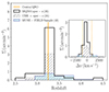 |
Fig. 5. Redshift distributions of the MQN01 high-confidence spectroscopic sample (black histogram) and of the UBR-selected LBGs with secure spectroscopic redshift from MUSE (hatched gray histogram). These are compared to the “MUSE-FIELD” sample and normalized by the surveyed area. The redshift of the central QSO is marked by an orange vertical line. The inset shows the velocity distribution of the MUSE galaxies and of the LBGs relative to the redshift of the QSO. The line-of-sight velocity window corresponding to |Δv|≤1000 km s−1 is highlighted by dotted vertical lines. |
4.2. Luminosity function and amplitude of the overdensity
Once established that an excess of star-forming galaxies is found in proximity to the QSO, we now provide a more statistical argument to investigate the amplitude of the overdensity relative to blank fields. We thus compute the cumulative luminosity function (LF), ϕc(< MR), defined as the number density of galaxies as a function of their luminosity. To account for the difference in redshift compared to the surveys available in the literature, we convert the flux measured in the R-band into absolute magnitude, MR. To obtain the cumulative luminosity function, we first compute the differential number of galaxies at a given magnitude and per unit volume within nine intervals of ΔMR = 0.175 mag and associate uncertainties from Poisson statistics. The differential measure is then integrated along the magnitude axis. We apply this procedure for the sample of 21 galaxies spectroscopically identified to lie within |Δv|≤1000 km s−1 around the redshift of the QSO. The results are shown in Figure 6. We produce the cumulative luminosity function also for the “MUSE-FIELD” sample of galaxies in the range 3.0 ≤ z ≤ 3.5 following the same steps described above. For these galaxies, the MR magnitude is estimated by convolving their spectra with the transmission curve of the FORS2/Rspecial filter. Similarly, we also produce the cumulative luminosity function for all the galaxies identified in the MUSE mosaic within 2.5 < z < 4.5, masking the peak of the overdensity in velocity space around the QSO. The luminosity functions of these two independent field samples are consistent with each other, both in shape and normalization. The consistency of the comparison is achieved by having searched for the galaxies in the same MUSE datacube or in those with similar exposure time, ≈10 h, and applying the same method and constraints to select only the sources with a precise measure of their spectroscopic redshift. On these bases, we assume the selection function to be the same across the samples and do not apply any completeness corrections to the above luminosity functions. In addition, we show that the normalization of the luminosity function of the field and control sample is consistent with results derived in the ℛ-band by Reddy & Steidel (2009) for a sample of color-selected LBGs with a spectroscopic redshift in the range 2.7 ≤ z < 3.4. However, our luminosity function is flatter due to the lack of corrections for completeness and selection effects. Specifically, requiring rest-frame UV absorption lines in the spectra biases against faint galaxies, which are underrepresented in our field and control samples compared to Reddy & Steidel (2009).
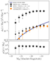 |
Fig. 6. Luminosity functions and overdensity of galaxies identified around the central QSO. Upper panel: cumulative R-band luminosity function of the MQN01 galaxies found within |Δv|≤1000 km s−1 from the redshift of the QSO (black stars), compared to that of the “MUSE-FIELD” sample (black pentagons) and of the control sample of sources found in the MQN01 MUSE FoV within 2.5 < z < 4.5, masking |Δv|≤1500 km s−1 around the QSO (orange diamonds). The vertical dotted line shows the magnitude at which the luminosity function of the spectroscopic samples flattens relative to the completeness-corrected one from Reddy & Steidel (2009). Lower panel: overdensity as a function of the R-band magnitude. |
To statistically measure the amplitude of the overdensity around the QSO, we take the ratio5 between the cumulative luminosity function and the one from Reddy & Steidel (2009). As shown in Figure 6 (lower panel), we measure an overdensity  at MR ≤ −19.25 mag. We also note that the overdensity is flat as a function of the magnitude threshold up to MR = −19.5 mag and declines at fainter magnitudes due to the incompleteness of the sample. This suggests that, on average, we only find a shift in the normalization of the luminosity function and do not observe any excess of bright or faint galaxies in the environment around the QSO compared to the field. We also performed the same analysis for the sample of color-selected LBGs and show the derived rest-frame UV luminosity functions in Appendix B.
4.3. Clustering analysis
Comparing the correlation length of the galaxies clustered around different QSOs at similar redshifts encodes key information about the structures in which they are hosted. We follow the formalism from Trainor & Steidel (2012), TS12 hereafter, and derive the galaxy-galaxy auto-correlation function, wGG, and the QSO-galaxies cross-correlation function, wQG. In three dimensions, the correlation functions are typically modeled by a power law, ξ = (r/r0)−γ, where γ is the slope and r0 is the correlation length. Once integrated in the redshift direction, the projected correlation functions take a functional form that still depends on the parameters γ and r0 (see Eq. (10) in TS12). In each radial bin, we compute wGG, QG(R) = (Nobs/Nexp)−1, where Nobs is the observed number of galaxies identified within a radial bin and Nexp is the expected one, derived from the luminosity functions of the field sample from Section 4.2. To compute the galaxy-galaxy auto-correlation function without being affected by the presence of the QSO in our field, we took the 2.5 < z < 4.5 galaxies with spectroscopic redshift measured from rest-frame UV absorption lines, that is, similar to our selection in Section 3.2, from the UDF catalog (Bacon et al. 2023). In addition, we proved this result to be consistent with upper limits for the auto-correlation of the galaxies identified in our field at 2.5 < z < 4.5, masking |Δv|≤1500 km s−1 around the redshift of the QSO. The results are shown in Figure 7, with the horizontal errorbars marking the width of each radial bin and the vertical ones derived from the 16th and 84th percentile of the distributions obtained by bootstrapping over the sample of galaxies. We derive the correlation length by fitting the equation 10 from TS12 to the data. The slope, γ, is degenerate with the correlation length and therefore fixed to different values to facilitate consistent comparisons with the literature. The best-fit results are shown in Figure 7 and listed in Table 4. The uncertainties are obtained from the 16th and 84th percentiles of the bootstrap distributions. The cross-correlation length estimated for spectroscopically selected star forming galaxies in MQN01 is substantially higher than the galaxy-galaxy correlation lengths obtained using the same selection and higher than the values found around other QSOs in the literature at similar times, e.g. compared to TS12. In Section 5.1, we discuss the implications of these results.
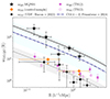 |
Fig. 7. Projected correlation functions assuming fixed γ = 1.8 and linking window |Δv|≤1000 km s−1. The QSO-galaxy cross-correlation function for the MUSE spectroscopic sample (black stars) is similar to that of CO(4–3) line emitters identified by Pensabene et al. (2024) in the same volume (blue line and shaded area), but significantly above that of Trainor & Steidel (2012) (purple, filled points). The galaxy-galaxy auto-correlation function is shown for the control-field sample of z = 2.5 − 4.5 galaxies identified in the UDF (black pentagons, Bacon et al. 2023), together with upper limits for the galaxies in our field within the same redshift range, but masking |Δv|≤1500 km s−1 around the redshift of the QSO (orange diamonds). Both the estimates are consistent with Trainor & Steidel (2012) (purple, empty points). The best-fit results are shown as dotted and solid lines for the auto and cross-correlation functions, respectively. All the uncertainties are derived from the 16th and 84th percentiles from bootstrap distributions. |
QSO-galaxies cross-correlation and galaxy-galaxy auto-correlation lengths.
4.4. Galaxies’ star formation activity compared to the field
How the large-scale environment affects galaxy growth is a key question within the framework of galaxy evolution in a hierarchical universe, especially in overdense regions throughout cosmic time. A useful approach to gauge galaxies’ ability to accrete cold gas and sustain star formation is by looking at their positioning in the stellar mass versus star formation rate (or specific star formation rate, sSFR) plane relative to the “main sequence” (see e.g., Brinchmann et al. 2004; Daddi et al. 2007; Elbaz et al. 2007; Noeske et al. 2007; Salim et al. 2007).
In Figure 8 we directly compare the SFR (left panel) and the sSFR (right panel) as a function of galaxies’ stellar mass derived for the galaxies clustered around the QSO with the star-forming main sequence at z ≈ 3.25. We parametrized the main sequence with the functional forms from Speagle et al. (2014) (blue), Popesso et al. (2023) (green) and Koprowski et al. (2024) (purple) at the QSO redshift, allowing for a 0.3 dex dispersion. The method we used to identify the galaxies (Section 3.2) selects rest-frame UV bright sources, that is, actively star forming and not too heavily obscured by dust. In other words, our selection tends to exclude passive or extremely red galaxies. As a result, at a given stellar mass, we do not observe any significant offset from the main sequence calibrated on blank fields at z ≈ 3 for the clustered galaxies, nor for the AGNs detected by Chandra (yellow squares in Figure 8). However, we notice that most massive galaxies clustered around the QSO host an AGN. Discussing the details and the implications of this finding are beyond the scope of this paper, and we refer the reader to Travascio et al. (2025) for a detailed study of the AGNs populating this structure. The evidence that galaxies form stars at main sequence rates seems to be a recurrent feature in some of the known z ≈ 2 − 3 protoclusters (see e.g., Koyama et al. 2013a,b; Cooke et al. 2014; Shimakawa et al. 2018a,b; Shi et al. 2019a,b, 2020; Toshikawa et al. 2024).
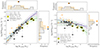 |
Fig. 8. Star-forming main sequence, in terms of SFR (left panel) and sSFR (right panel), of the MQN01 galaxies clustered around the QSO (black stars), compared to the control-field sample (orange diamonds). The data are compared to the main sequence at z ≈ 3.25 derived from Speagle et al. (2014) (blue), Popesso et al. (2023) (green) and Koprowski et al. (2024) (purple). The X-Ray detected AGN are marked by yellow squares. The histograms on the top and right panels show the distribution of the SFR or sSFR and galaxies’ stellar mass, respectively, of the MQN01 galaxies (black) and of the control-field sample, together with their median values on top. |
Due to the differences in the selection function and in the SFR estimates between the sample of MQN01 galaxies and the ones used to calibrate the parametrizations of the main sequence, it is more informative to directly compare the properties of the galaxies in the overdensity to those included in a field sample with a similar selection function. To this end, we consider the control-field sample of 11 galaxies identified in the MUSE FoV (see Section 3.3). All these galaxies are scattered along the expected main sequence. In addition, we compare the distributions of stellar mass (top panels), SFR and sSFR (right panels) shown in Figure 8 by performing a KS test (significant at 2σ level for p-values ≤ 0.05). While the distributions of sSFR are unlikely drawn from the same parent one, p−value ≈ 0.01, there is no statistical difference in those of stellar mass and SFR (p-value ≈ 0.35 and p−value ≈ 0.45, respectively). Nonetheless, we notice that we find only one galaxy in the field sample located in the log(M⋆/M⊙) ≳ 10.5 region of the main sequence, and it is possibly the excess of galaxies in the high-mass tail of the distribution that is driving the difference in the sSFR. The direct comparison between the distributions of the two samples does not take into account the different encompassing co-moving volume (≈2 × 10⁴ cMpc3 for the field sample, which is more than 50 times larger compared to that of the sample of galaxies clustered around the QSO). Normalizing the number of sources by the co-moving volume, we find that the number density of massive (M⋆ ≳ 1010.5 M⊙) star forming galaxies is  times higher around the QSO than in a blank field. Even accounting for the overdensity of ≈53 measured around the QSO in Section 4.2, the presence of massive galaxies exceeds by a factor of
  the expectations for the field (see, Section 9 for details). On the other hand, the incidence of M⋆ ≲ 1010.5 M⊙ galaxies around the QSO is
  times larger than in the field sample, which corresponds to a factor of
  once accounting for the overdensity. These results also corresponds to a factor of
  more galaxies forming stars at a rate log[SFR/(M⊙ yr−1)] ≥ 1.7 around the QSO compared to blank fields. In terms of sSFR, the massive star-forming galaxies discussed above reside at log(sSFR/yr−1) < −8.5, leading to a large overdensity (
 ) in this sSFR range as well. This scenario is thus consistent with a picture where a consistent fraction of galaxies in this overdense environment is experiencing a phase of accelerated mass assembly and is rapidly consuming its gas content.
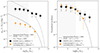 |
Fig. 9. Excess of massive log(M⋆/M⊙)≳10.5 galaxies around the MQN01 QSO. Left panel: cumulative stellar mass function of the MQN01 spectroscopic sample in proximity to the QSO (black stars) compared to the control-field sample (orange diamonds) and the expectations for blank fields from the COSMOS survey (3.0 < z < 3.5, Weaver et al. 2023, gray). Right panel: same as the left panel, but normalized to the value of the cumulative mass function at M⋆ = 109.8 M⊙, corresponding to the 90% completeness limit of the MQN01 spectroscopic sample. |
4.5. Galaxies’ stellar mass function
Motivated by the results obtained in Section 4.4, we now compute the galaxies’ number density as a function of their stellar mass by integrating the differential stellar mass function and propagating the Poisson errors arising in each interval of masses. To also take into account the errors in the measure of the stellar mass itself, we bootstrap varying the fiducial values within the uncertainties derived from the galaxies’ SED fitting 1000 times. The standard deviation from the 16th and 84th percentiles of the resulting bootstrap distribution is then squared and summed with errors propagated from the integral above. In the left panel in Figure 9 we show the resulting cumulative stellar mass function, while in the right panel we normalize it at the stellar mass completeness limit6 to better capture any difference in shape. The estimate for the galaxies around the QSO (black stars) is compared to the expectations for different field samples. We thus take as a reference the stellar mass function computed by Weaver et al. (2023) in the COSMOS2020 field within the redshift range 3.0 < z < 3.5 and rescale it by the MQN01 overdensity  . This is also consistent with what we obtained for the galaxies included in the control-field sample and identified within the redshift range 2.5 < z < 4.5, masking the peak of the overdensity in velocity space (orange diamonds). While both the stellar mass functions flatten and deviate from Weaver et al. (2023) field expectations at log(M⋆/M⊙)≲9.5, likely due to the incompleteness of the samples, that of star-forming galaxies clustered with the QSO is also flatter at masses log(M⋆/M⊙)≳10.5. In other words, this change in the shape of the stellar mass function provides evidence that the surroundings of the QSO are richer in massive galaxies compared to the field, with 4 ± 2 and 24 ± 11 times more sources in the two bins at log(M⋆/M⊙)≳10.5, respectively, once accounted for the overdensity.
4.6. Connecting the local overdense environment to the galaxy properties
We now turn to investigate how the properties of the galaxies depend on the local overdensity. We thus employ a scale-independent Voronoi Tessellation (one element per cell) to parametrize the local density of galaxies clustered around the QSO. According to this criterion, the size of each cell is, by construction, inversely proportional to the local galaxy surface density (i.e., small cells correspond to crowded environments). Open cells at the edge of the FoV (7/21) are excluded from the analysis due to the unavailable information about the objects located outside the MUSE mosaic. The overdensity is then defined as  (so that log(1 + Δ) = 0 corresponds to the case in which the galaxy density is the same as the field, i.e.,
  ). We show in Figure 10 how the SFR, stellar mass and sSFR correlate with the local galaxy density. To address this analysis on a more statistical basis, we also performed a Spearman-rank correlation test and report in Table 5 the strength of the correlation, ρspearman, and the probability that no monotonic relation exists between the two variables, p-value. We require p-value ≤ 0.05 for a correlation to be significant at least at 2σ confidence level. As a result, we observe that the galaxies’ stellar mass and sSFR are positively and negatively, respectively, correlated (|ρspearman|≳0.45 and p-value ≈ 0.05) with the local density at 2σ significance. On the other hand, we do not observe any significant environmental effect on the SFR itself (p−value ≈ 0.29).
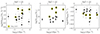 |
Fig. 10. MQN01 galaxies’ SFR (1st panel), stellar mass (2nd panel) and sSFR (3rd panel) as a function of the co-moving local galaxy density (bottom x-axis) and overdensity (top x-axis) with respect to the field. X-Ray emitting AGN detected in Chandra observations are highlighted as yellow squares. |
Results of the Spearman-rank test on the correlations between the properties of the MQN01 galaxies and the local overdensity.
4.7. Probing the structure on larger scales
The large-scale structures in which galaxies are embedded are expected to extend well beyond the ≈4 × 4 cMpc2 we are able to trace with the star-forming galaxies identified within the FoV of the MUSE mosaic. We thus model the 2D spatial distribution of the UBR-selected LBGs across the ≈24 × 24 cMpc2 FoV of FORS2 and compare it to that of the spectroscopically selected sources lying within |Δv|≤1000 km s−1 from the QSO in the 4 × 4 cMpc2 FoV of the MUSE mosaic. This is done by creating an evenly spaced grid of 7″ × 7″ and 5″ × 5″ cells covering the entire FORS2 and MUSE FoV, respectively. The number of galaxies identified within each cell is then normalized by the volume of the cell and compared to the co-moving density expected for the field sample (see Section 4.2). The grid is then oversampled (by a factor of 3 and 2, respectively) and smoothed with a Gaussian Kernel (σ = 6, 5, respectively, corresponding to ≈0.5″). Results are shown in Figure 11.
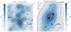 |
Fig. 11. 2D overdensity maps of the LBGs and of the spectroscopically selected galaxies found to be clustered with the QSO. Left panel: Overdensity map of the LBGs identified within the 24 × 24 cMpc2 FORS2 FoV. The amplitude of the overdensity is shown in shades of blue scaling with the colormap. Contours are shown for |

The LBGs appear to be mildly overdense ( ) across a large fraction of the ≈24 × 24 cMpc2 FoV, even at large distances from the central QSO. The overdense regions
  are concentrated closer to the center of the field and show a preferential vertical orientation, which corresponds to the north-south direction on the sky, and is also aligned with both the overdensity of spectroscopically selected galaxies that we observe in MUSE (right panel) and the extended Lyα emitting gas observed by Borisova et al. (2016) and Cantalupo et al. (in prep.). This evidence supports a picture in which the large-scale structure traced by the galaxies clustered with the QSO extends well beyond the FoV of the MUSE mosaic, for tens of comoving megaparsecs. We reserve a more statistical treatment of the LBGs alignment as a function of the local overdensity to Appendix C. On the other hand, when looking at this structure on scales of 24 × 24 cMpc2, we observe that the most overdense regions,
  , are not found within the FoV of the MUSE mosaic, but are mostly concentrated in the southern part of the field. Some possible scenarios, or a combination of them, should be tested to explain this evidence: (i) they are part of a foreground or background structure; (ii) the structure surrounding the QSO itself extends in the southern direction; (iii) despite being close to the peak of the overdensity in the MUSE FoV, the QSO is not the center of the structure, which is instead in the South; (iv) they are tracing two merging or interacting structures. Spectroscopic confirmation of LBGs would be essential to discriminate between these scenarios.
5. Discussion
In this section, we put the results presented above into a broader context by comparing them to previous results available in the literature. In particular, in Section 5.1 we discuss the overdensity and clustering measurements in MQN01 in light of other studies targeting QSOs and overdense regions at z > 2. In Section 5.2, we focus on the galaxies’ sSFR and stellar mass function in MQN01 comparing them to other works from the literature, both in the field and in overdense regions, to reveal the possible role of the local environment on galaxy formation and evolution.
5.1. MQN01 overdensity and clustering compared to other fields
The number of galaxies spectroscopically confirmed to be within |Δv|≤1000 km s−1 and in an area of ≈4 × 4 cMpc2 (≈ 2 × 2 arcmin2) around the MQN01 QSO results in an overdensity of  which corresponds to a surface density of ≈1.3 cMpc−2. At a redshift similar to that of MQN01, several galaxy overdensities and protoclusters have been studied in the literature, such as SSA22 at z ≈ 3.08 (Steidel et al. 1998, 2003), Hyperion at z ≈ 2.47 (Cucciati et al. 2018) and Spiderweb at z ≈ 2.15 (Roettgering et al. 1994; Pentericci et al. 1997). In particular, Topping et al. (2016) found 40 LBGs in SSA22 with spectroscopic redshift in the range z = 3.05 − 3.12 across 17.25 × 17.25 cMpc2, which result in a surface density of ≈0.13 cMpc−2. Huang et al. (2022) discovered 53 Lyα emitters in a region extended over ≈30 × 20 cMpc2 in Hyperion, with a surface density of ≈0.08 cMpc−1. In Spiderweb, Pérez-Martínez et al. (2023) found 39 spectroscopically confirmed Hα emitters across 13.7 × 19.3 cMpc2, corresponding to a surface density of ≈0.15 cMpc−1. Notably, the surface density measured in the MQN01 field is ≈10 − 20 times higher with respect to these structures. A direct comparison, however, is not straightforward given the different galaxy populations selected in these works, the different levels of completeness reached and the surveyed volumes. A detailed comparison would require, for instance, a MUSE (or KCWI) survey in these proto-cluster fields, similar to the one performed around MQN01.
Besides the large overdensity of star-forming galaxies in the field, a significant excess of galaxies in MQN01 obtained with different tracers has been reported. In particular, Pensabene et al. (2024) found ≈18 times more CO(4–3) line emitters and higher 1.2mm source number counts compared to blank fields, with the latter result that is similar to the findings in SSA22. Exploring Chandra X-Ray data, an overdensity of  of AGNs has recently been unveiled by Travascio et al. (2025) and found to exceed that observed in SSA22 and Spiderweb protoclusters. These studies support the peculiarity of the MQN01 field in terms of galaxy overdensity as suggested by our spectroscopic study in the rest-frame UV.
Stronger evidence about the rarity of the MQN01 structure is obtained by the cross-correlation function presented in Section 4.3. In particular, we obtained a QSO-galaxy cross-correlation length of  , which is significantly higher than the galaxy-galaxy correlation length of
  for fixed γ = 1.8. Despite the limited statistics, the cross-correlation lengths obtained using CO(4–3) line emitters around the MQN01 by Pensabene et al. (2024),
  , are also consistent with these values. These values clearly indicate that galaxies in the MQN01 structure are more clustered around the QSO compared to both the average fields and other QSOs at similar redshifts (see, e.g., Trainor & Steidel 2012; Garcia-Vergara 2021). For consistency and to control for the effects of different selection functions, we compare our results with works that studied the clustering of similar samples of galaxies, within similar volumes and at similar redshifts. TS12 measured an auto-correlation length r0 = (5.8 ± 1.3) h−1 cMpc and a cross-correlation length r0 = (7.1 ± 1.3) h−1 cMpc (once rescaled to the cosmology adopted in this paper, which corresponds to a correction factor of 1.03), assuming γ = 1.5, for a spectroscopic sample of galaxies identified within ±1500 km s−1 from 15 QSOs at z ≈ 2.7. The auto-correlation functions of galaxies selected as those found in MQN01, are consistent with that of TS12 (see Table 4). On the other hand, the cross-correlation lengths of the galaxies identified within |Δv|≤1500 km s−1 around the QSO is ≈3.2 times larger compared to TS12. We also measured the QSO-galaxy cross-correlation function in the MAGG survey (Lofthouse et al. 2020), which includes 28 fields centered on QSOs and observed with MUSE (see Appendix D for more details). For consistency with the sample of galaxies used in this work, we considered only those that have been continuum-selected, as described in Lofthouse et al. (2020), brighter than mR ≤ 26.5 mag, with a secure measure of their spectroscopic redshifts and found within |Δv|≤1500 km s−1 from the redshift of each MAGG QSO (median z ≈ 3.7). We derived a cross-correlation length of r0 = (3.8 ± 0.8) h−1 cMpc for fixed γ = 1.5. Interestingly, the one measured in the MQN01 field is ≈6 times larger. Altogether, these pieces of evidence suggest that the MQN01 QSO could possibly be associated with a much larger halo than the typical QSO host at these redshifts, which is estimated to be around log(Mh/M⊙)≈12 − 12.5 (TS12, see also, Fossati et al. 2021; Arrigoni Battaia et al. 2022; de Beer et al. 2023).
5.2. The role of the local environment on galaxy formation and evolution
One of the key results presented in Section 4.5 is the fact that the galaxy overdensity in the MQN01 field depends on the galaxy stellar mass. In particular, Figure 9 shows that there is an elevated fraction of massive galaxies compared to the expectations from average regions of the Universe, suggesting a possible link between the environment and galaxy growth. Indeed, despite the limited statistics, we find a hint that the local galaxy overdensity is positively correlated with the galaxies’ stellar mass (and negatively correlated with their sSFR) as shown in Figure 10. Our results reinforce previous findings in the literature (see e.g., Darvish et al. 2016; Chartab et al. 2020; Lemaux et al. 2022; Taamoli et al. 2024), which did not have the large dynamic range in overdensity as provided by our sample.
For instance, by using a large sample of protocluster candidates, Toshikawa et al. (2024) found that U-dropout galaxies living in overdense regions at z ≈ 3 show a cumulative stellar mass function that is flatter at the massive end compared to the field. Similarly, Shimakawa et al. (2018a,b) found a statistically significant excess of massive galaxies in two z ≈ 2 protoclusters, broadly consistent with other studies of continuum-selected galaxies and Hα emitters in overdense regions at similar redshifts (see e.g., Steidel et al. 2005; Koyama et al. 2013a,b; Cooke et al. 2014). However, they also observe that such massive galaxies are mostly located in the densest regions of the protocluster, while sources in less dense areas have a stellar mass function distribution that is more similar to that of the field (see also, Forrest et al. 2024, at 3.20 < z < 3.45).
The presence of an excess of massive galaxies in overdense regions, such as protoclusters, can be supported by different scenarios: (i) the high density environment can trigger mergers as well as boost the rate of interactions between galaxies (e.g., Alonso et al. 2012; Cooke et al. 2014; D’Amato et al. 2020; ii) the access to a large gas reservoir that is efficiently accreted from the cosmic web onto the galaxies (see e.g., Shimakawa et al. 2018a). Indeed, Umehata et al. (2019) found that AGNs and submillimeter galaxies in the SSA22 protocluster are located within filaments of gas, which can potentially be accreted by these sources fuelling their star formation and driving their growth. On the other hand, there is also evidence that overdensities play a minor role in shaping the scaling relations of galaxies at z > 2 (see e.g., McGee et al. 2009; Fossati et al. 2017), which requires further investigation to be conducted in similar regions of the Universe. Altogether, these possible scenarios suggest that these galaxies grew rapidly, either assembling their masses earlier or more efficiently than those in the field.
5.3. Caveats and future prospects
The most important step for a more complete view of the galaxy population in MQN01 is the inclusion of the passive galaxies. One possibility to select them would require, for instance, properly sampling the Balmer break, expected to be in the H-band at the MQN01 redshift. Photometric data obtained with VLT/HAWK-I are currently available and will be used in a future study to complement the dataset presented here. In addition, JWST spectra covering the Balmer lines at rest-frame wavelengths from 400 to 700 nm are available for some galaxies in the field (Cantalupo et al. 2021; Wang et al. 2024b). However, for a more complete view of the passive galaxy population, grism JWST spectroscopy would be necessary. Only a small area of the MQN01 structure, as probed through our LBG survey, currently has MUSE coverage and thus spectroscopic confirmation. An ongoing MUSE survey (Program ID 112.25N3, PI S. Cantalupo) is covering ≈14 cMpc in the north-south direction and will be used to extend the study of the clustering and the galaxies’ properties up to the outskirt of the structure. Finally, our findings are limited to one individual and rare structure, which prevents us from generalizing them to the broader population of protoclusters. To identify a larger number of systems similar to MQN01 and study their galaxy populations, it would be necessary to conduct systematic deep and wide surveys, for instance with MUSE or KCWI, targeting extended QSO nebulae as signposts for these structures.
6. Summary and conclusions
We detected and studied a population of star-forming galaxies clustered within ≈4 × 4 cMpc2 around the z ≈ 3.25 QSO CTS G18.01, known as MQN01 field. The QSO is surrounded by a giant Lyα emitting nebula discovered by Borisova et al. (2016) and Cantalupo et al. (in prep.), and the field hosts a large overdensity of dusty star-forming galaxies (Pensabene et al. 2024) and AGNs (Travascio et al. 2025). By leveraging a rich set of multiwavelength data, including MUSE, FORS2, HAWK-I, HST, JWST and Chandra, we derived the SFRs and the stellar masses of these galaxies and explored their connection to the local and large-scale overdense environment. The key results are summarized below:
-
We discovered an overdensity of star forming galaxies of
 clustered within 4 × 4 cMpc2 and |Δv|≤1000 km s−1 around the central QSO. Measuring the amplitude of the clustering as a function of the projected distance from the QSO, we derived a cross-correlation length that is ≈3.2 times larger than the average value found by Trainor & Steidel (2012) for z ≈ 2.7 QSOs. Galaxies in this structure are thus either more clustered or living in a more massive structure than those observed around average QSOs at similar times.
 -
We found that the galaxies in the overdensity are forming stars at a rate consistent with the expected main sequence at z ≈ 3.25. In addition, the ability of these galaxies to form stars appears to be more sensitive to the gas and baryon content of the galaxies, probed by their stellar masses, rather than to the local overdensities and the large-scale environment in which they reside.
-
At the high-mass end, the cumulative stellar mass function is flatter compared to the field. This suggests the presence of an excess of massive galaxies in the structure, with ≈4 times higher number density than in the field at log(M⋆/M⊙)≥10.5. In addition, all the massive galaxies are also X-Ray AGNs. Such an excess of massive star forming galaxies may be due to a higher merger rate or efficient accretion that allows the galaxies to assemble their mass at earlier times or more efficiently than in the field and provide them enough fuel to continue forming stars at main sequence rates.
-
The distribution of color-selected LBGs on scales ×36 larger than the original FoV of the MUSE mosaic suggests that the overdensity extends along the north-south direction and is thus aligned with the Lyα emitting gas detected by Borisova et al. (2016) around the QSO and to the ≈4 cMpc filamentary structure observed in emission by Cantalupo et al. (in prep.) This may be a hint that the gaseous structure in which galaxies are embedded extends for tens of comoving megaparsecs.
Overdense structures, such as MQN01, are ideal places to explore the possible connection between the environment and the properties of galaxies at high redshift. The advancement in the study of overdensities at z > 2 made it possible to explore a wide range of environments, even at cosmic noon. However, given their rarity, it is still challenging to build a large sample of such structures, and thus to increase the statistical significance of any possible connection between galaxies and the environment. As such, even if based on a single field, our study provides important clues for future investigations to piece together the coevolution of galaxies and their large-scale environments from the very early epochs to the late times.
The final, combined cube consists of a 2 × 2 mosaic of 4 pointings. All of these overlap in a small region ≈60 kpc away from the QSO, where the integrated exposure time is 20 h. In all the other regions it ranges from 8 h, at the edges, to 12 h.
The photometric calibration of the B-band and R-band observations is done with the extinction-corrected instrumental zero-point available on the ESO data quality-control database (http://archive.eso.org/qc1/qc1_cgi). These measurements were processed using the ESO pipeline by combining standard star observations taken for at least 7 stable nights around the nights of the observations. For the U-band images, instead, we run the ESO pipeline on the daily standard frames to measure the zero-point.
We employed the luminosity functions to measure the expected number density of galaxies for blank fields. For the sample of LBGs, we integrated R-band luminosity function of Reddy et al. (2008) and multiplied it by the completeness curve of the FORS2/R-band (see Figure 1) to account for the selection function of our sample. For the sample of spectroscopically selected galaxies, instead, such value was directly taken from the luminosity function of the “MUSE-FIELD” sample (which is also consistent, within 1σ uncertainty, to the estimates from the luminosity function of Reddy & Steidel (2009) and that of the control-field sample we built masking the overdensity around the QSO). As a result, we measured a co-moving density in blank fields to be  and
and  for the color-selected LBGs and the MUSE spectroscopic sample, respectively.
To estimate an order-of-magnitude completeness for the MUSE spectroscopic samples, we adopt the empirical method from Pozzetti et al. (2010), Davidzon et al. (2013), Ilbert et al. (2013), Moustakas et al. (2013), Laigle et al. (2016), which has already been applied by Toshikawa et al. (2024) on U-dropout galaxies at z ≈ 3. With a K-band magnitude limit of 25.5 mag (see Section 2.3), we estimate that our sample is 90% complete at log(M⋆/M⊙)≈9.8.
The set of models is publicly available at http://www.bruzual.org/CB19/. A detailed description is provided in Appendix A of Sánchez et al. (2022).
Acknowledgments
We thank the anonymous referee for the careful reading of the paper and for useful suggestions that improved the manuscript. This project was supported by the European Research Council (ERC) Consolidator Grant 864361 (CosmicWeb) and by Fondazione Cariplo grant no. 2020-0902. MiF gratefully acknowledges support from the European Research Council (ERC) under the European Union’s Horizon 2020 research and innovation programme (grant agreement no. 757535) and by Fondazione Cariplo, grant no. 2018-2329. This work is based on observations collected at the European Southern Observatory under ESO programmes IDs 102.A-0448(A), and 110.23ZX. This work made use of Astropy (http://www.astropy.org) a community-developed core Python package and an ecosystem of tools and resources for astronomy (Astropy Collaboration 2013, 2018, 2022), Numpy (Harris et al. 2020), SciPy (Virtanen et al. 2020), and Matplotlib (Hunter 2007).
References
- Adams, S. M., Martini, P., Croxall, K. V., Overzier, R. A., & Silverman, J. D. 2015, MNRAS, 448, 1335 [NASA ADS] [CrossRef] [Google Scholar]
- Alberts, S., & Noble, A. 2022, Universe, 8, 554 [Google Scholar]
- Alonso, S., Mesa, V., Padilla, N., & Lambas, D. G. 2012, A&A, 539, A46 [NASA ADS] [CrossRef] [EDP Sciences] [Google Scholar]
- Alpaslan, M., Robotham, A. S. G., Driver, S., et al. 2014, MNRAS, 438, 177 [Google Scholar]
- Appenzeller, I., Fricke, K., Fürtig, W., et al. 1998, The Messenger, 94, 1 [NASA ADS] [Google Scholar]
- Arrigoni Battaia, F., Chen, C.-C., Liu, H.-Y. B., et al. 2022, ApJ, 930, 72 [NASA ADS] [CrossRef] [Google Scholar]
- Asplund, M., Grevesse, N., Sauval, A. J., & Scott, P. 2009, ARA&A, 47, 481 [NASA ADS] [CrossRef] [Google Scholar]
- Assef, R. J., Eisenhardt, P. R. M., Stern, D., et al. 2015, ApJ, 804, 27 [Google Scholar]
- Astropy Collaboration (Robitaille, T. P., et al.) 2013, A&A, 558, A33 [NASA ADS] [CrossRef] [EDP Sciences] [Google Scholar]
- Astropy Collaboration (Price-Whelan, A. M., et al.) 2018, AJ, 156, 123 [Google Scholar]
- Astropy Collaboration (Price-Whelan, A. M., et al.) 2022, ApJ, 935, 167 [NASA ADS] [CrossRef] [Google Scholar]
- Bacon, R., Accardo, M., Adjali, L., et al. 2010, in Ground-based and Airborne Instrumentation for Astronomy III, eds. I. S. McLean, S. K. Ramsay, & H. Takami, Society of Photo-Optical Instrumentation Engineers (SPIE) Conference Series, 7735, 773508 [Google Scholar]
- Bacon, R., Brinchmann, J., Richard, J., et al. 2015, A&A, 575, A75 [NASA ADS] [CrossRef] [EDP Sciences] [Google Scholar]
- Bacon, R., Conseil, S., Mary, D., et al. 2017, A&A, 608, A1 [NASA ADS] [CrossRef] [EDP Sciences] [Google Scholar]
- Bacon, R., Brinchmann, J., Conseil, S., et al. 2023, A&A, 670, A4 [NASA ADS] [CrossRef] [EDP Sciences] [Google Scholar]
- Baldry, I. K., Balogh, M. L., Bower, R. G., et al. 2006, MNRAS, 373, 469 [Google Scholar]
- Bamford, S. P., Nichol, R. C., Baldry, I. K., et al. 2009, MNRAS, 393, 1324 [NASA ADS] [CrossRef] [Google Scholar]
- Bañados, E., Venemans, B., Walter, F., et al. 2013, ApJ, 773, 178 [CrossRef] [Google Scholar]
- Barrufet, L., Pearson, C., Serjeant, S., et al. 2020, A&A, 641, A129 [NASA ADS] [CrossRef] [EDP Sciences] [Google Scholar]
- Bertin, E. 2006, in Astronomical Data Analysis Software and Systems XV, 351, 112 [NASA ADS] [Google Scholar]
- Bertin, E. 2010, Astrophysics Source Code Library [record ascl:1010.068] [Google Scholar]
- Bertin, E. 2011, in Astronomical Data Analysis Software and Systems XX, eds. I. N. Evans, A. Accomazzi, D. J. Mink, & A. H. Rots, Astronomical Society of the Pacific Conference Series, 442, 435 [Google Scholar]
- Bertin, E., & Arnouts, S. 1996, A&AS, 117, 393 [NASA ADS] [CrossRef] [EDP Sciences] [Google Scholar]
- Bielby, R. M., Shanks, T., Weilbacher, P. M., et al. 2011, MNRAS, 414, 2 [Google Scholar]
- Bielby, R. M., Stott, J. P., Cullen, F., et al. 2019, MNRAS, 486, 21 [CrossRef] [Google Scholar]
- Bond, J. R., Kofman, L., & Pogosyan, D. 1996, Nature, 380, 603 [NASA ADS] [CrossRef] [Google Scholar]
- Boquien, M., Burgarella, D., Roehlly, Y., et al. 2019, A&A, 622, A103 [NASA ADS] [CrossRef] [EDP Sciences] [Google Scholar]
- Borisova, E., Cantalupo, S., Lilly, S. J., et al. 2016, ApJ, 831, 39 [Google Scholar]
- Bradley, L., Sipőcz, B., Robitaille, T., et al. 2023, https://doi.org/10.5281/zenodo.1035865 [Google Scholar]
- Brinchmann, J., Charlot, S., White, S. D. M., et al. 2004, MNRAS, 351, 1151 [Google Scholar]
- Bruzual, G., & Charlot, S. 2003, MNRAS, 344, 1000 [NASA ADS] [CrossRef] [Google Scholar]
- Burgarella, D., Buat, V., & Iglesias-Páramo, J. 2005, MNRAS, 360, 1413 [NASA ADS] [CrossRef] [Google Scholar]
- Byler, N., Dalcanton, J. J., Conroy, C., et al. 2018, ApJ, 863, 14 [NASA ADS] [CrossRef] [Google Scholar]
- Calvi, R., Poggianti, B. M., Vulcani, B., & Fasano, G. 2013, MNRAS, 432, 3141 [NASA ADS] [CrossRef] [Google Scholar]
- Calzetti, D., Armus, L., Bohlin, R. C., et al. 2000, ApJ, 533, 682 [NASA ADS] [CrossRef] [Google Scholar]
- Cantalupo, S., Pezzulli, G., Lilly, S. J., et al. 2019, MNRAS, 483, 5188 [Google Scholar]
- Cantalupo, S., Fossati, M., Fumagalli, M., et al. 2021, Unraveling the knots of gaseous Cosmic Web filaments at z 3 through H-alpha emission observations JWST Proposal. Cycle 1, ID. #1835 [Google Scholar]
- Casali, M., Pirard, J. F., Kissler-Patig, M., et al. 2006, in Ground-based and Airborne Instrumentation for Astronomy, eds. I. S. McLean, & M. Iye, Society of Photo-Optical Instrumentation Engineers (SPIE) Conference Series, 6269, 62690W [NASA ADS] [CrossRef] [Google Scholar]
- Casey, C. M., Cooray, A., Capak, P., et al. 2015, ApJ, 808, L33 [NASA ADS] [CrossRef] [Google Scholar]
- Cen, R., & Ostriker, J. P. 2000, ApJ, 538, 83 [Google Scholar]
- Chabrier, G. 2003, PASP, 115, 763 [Google Scholar]
- Chapman, S. C., Blain, A., Ibata, R., et al. 2009, ApJ, 691, 560 [NASA ADS] [CrossRef] [Google Scholar]
- Chartab, N., Mobasher, B., Darvish, B., et al. 2020, ApJ, 890, 7 [NASA ADS] [CrossRef] [Google Scholar]
- Chiang, Y.-K., Overzier, R., & Gebhardt, K. 2013, ApJ, 779, 127 [Google Scholar]
- Chiang, Y.-K., Overzier, R. A., Gebhardt, K., & Henriques, B. 2017, ApJ, 844, L23 [Google Scholar]
- Conroy, C. 2013, ARA&A, 51, 393 [NASA ADS] [CrossRef] [Google Scholar]
- Contini, E., De Lucia, G., Hatch, N., Borgani, S., & Kang, X. 2016, MNRAS, 456, 1924 [NASA ADS] [CrossRef] [Google Scholar]
- Cooke, E. A., Hatch, N. A., Muldrew, S. I., Rigby, E. E., & Kurk, J. D. 2014, MNRAS, 440, 3262 [NASA ADS] [CrossRef] [Google Scholar]
- Cucciati, O., Lemaux, B. C., Zamorani, G., et al. 2018, A&A, 619, A49 [NASA ADS] [CrossRef] [EDP Sciences] [Google Scholar]
- Daddi, E., Dickinson, M., Morrison, G., et al. 2007, ApJ, 670, 156 [NASA ADS] [CrossRef] [Google Scholar]
- D’Amato, Q., Gilli, R., Prandoni, I., et al. 2020, A&A, 641, L6 [NASA ADS] [CrossRef] [EDP Sciences] [Google Scholar]
- Darvish, B., Mobasher, B., Sobral, D., et al. 2016, ApJ, 825, 113 [NASA ADS] [CrossRef] [Google Scholar]
- Davidzon, I., Bolzonella, M., Coupon, J., et al. 2013, A&A, 558, A23 [NASA ADS] [CrossRef] [EDP Sciences] [Google Scholar]
- de Beer, S., Cantalupo, S., Travascio, A., et al. 2023, MNRAS, 526, 1850 [NASA ADS] [CrossRef] [Google Scholar]
- de Lapparent, V., Geller, M. J., & Huchra, J. P. 1986, ApJ, 302, L1 [Google Scholar]
- Di Mascolo, L., Saro, A., Mroczkowski, T., et al. 2023, Nature, 615, 809 [NASA ADS] [CrossRef] [Google Scholar]
- Elbaz, D., Daddi, E., Le Borgne, D., et al. 2007, A&A, 468, 33 [NASA ADS] [CrossRef] [EDP Sciences] [Google Scholar]
- ESO CPL Development Team 2015, Astrophysics Source Code Library [record ascl:1504.003] [Google Scholar]
- Falder, J. T., Stevens, J. A., Jarvis, M. J., et al. 2011, ApJ, 735, 123 [NASA ADS] [CrossRef] [Google Scholar]
- Ford, H. C., Bartko, F., Bely, P. Y., et al. 1998, in Space Telescopes and Instruments V, eds. P. Y. Bely, & J. B. Breckinridge, Society of Photo-Optical Instrumentation Engineers (SPIE) Conference Series, 3356, 234 [NASA ADS] [CrossRef] [Google Scholar]
- Forrest, B., Lemaux, B. C., Shah, E. A., et al. 2024, ApJ, 971, 169 [NASA ADS] [Google Scholar]
- Fossati, M., Wilman, D. J., Mendel, J. T., et al. 2017, ApJ, 835, 153 [Google Scholar]
- Fossati, M., Mendel, J. T., Boselli, A., et al. 2018, A&A, 614, A57 [NASA ADS] [CrossRef] [EDP Sciences] [Google Scholar]
- Fossati, M., Fumagalli, M., Lofthouse, E. K., et al. 2019, MNRAS, 490, 1451 [NASA ADS] [CrossRef] [Google Scholar]
- Fossati, M., Fumagalli, M., Lofthouse, E. K., et al. 2021, MNRAS, 503, 3044 [NASA ADS] [CrossRef] [Google Scholar]
- Fritz, J., Franceschini, A., & Hatziminaoglou, E. 2006, MNRAS, 366, 767 [Google Scholar]
- Gaia Collaboration (Prusti, T., et al.) 2016, A&A, 595, A1 [NASA ADS] [CrossRef] [EDP Sciences] [Google Scholar]
- Gaia Collaboration (Vallenari, A., et al.) 2023, A&A, 674, A1 [NASA ADS] [CrossRef] [EDP Sciences] [Google Scholar]
- Galbiati, M., Fumagalli, M., Fossati, M., et al. 2023, MNRAS, 524, 3474 [NASA ADS] [CrossRef] [Google Scholar]
- Galbiati, M., Dutta, R., Fumagalli, M., Fossati, M., & Cantalupo, S. 2024, A&A, 690, A7 [NASA ADS] [CrossRef] [EDP Sciences] [Google Scholar]
- Garcia-Vergara, C. 2021, https://doi.org/10.5281/zenodo.5005051 [Google Scholar]
- García-Vergara, C., Hennawi, J. F., Barrientos, L. F., & Rix, H.-W. 2017, ApJ, 848, 7 [CrossRef] [Google Scholar]
- Gatica, C., Demarco, R., Dole, H., et al. 2024, MNRAS, 527, 3006 [Google Scholar]
- Geller, M. J., & Huchra, J. P. 1989, Science, 246, 897 [NASA ADS] [CrossRef] [Google Scholar]
- Ginolfi, M., Piconcelli, E., Zappacosta, L., et al. 2022, Nat. Commun., 13, 4574 [NASA ADS] [CrossRef] [Google Scholar]
- Gonzaga, S., Hack, W., Fruchter, A., & Mack, J. 2012, The DrizzlePac Handbook (HST Data Handbook) [Google Scholar]
- Greenslade, J., Clements, D. L., Cheng, T., et al. 2018, MNRAS, 476, 3336 [NASA ADS] [CrossRef] [Google Scholar]
- Gu, M., Conroy, C., & Brammer, G. 2018, ApJ, 862, L18 [Google Scholar]
- Harris, C. R., Millman, K. J., van der Walt, S. J., et al. 2020, Nature, 585, 357 [NASA ADS] [CrossRef] [Google Scholar]
- Hatch, N. A., Wylezalek, D., Kurk, J. D., et al. 2014, MNRAS, 445, 280 [NASA ADS] [CrossRef] [Google Scholar]
- Hayashi, M., Kodama, T., Tadaki, K.-I., Koyama, Y., & Tanaka, I. 2012, ApJ, 757, 15 [NASA ADS] [CrossRef] [Google Scholar]
- Hayashino, T., Matsuda, Y., Tamura, H., et al. 2004, AJ, 128, 2073 [Google Scholar]
- Hennawi, J. F., Prochaska, J. X., Cantalupo, S., & Arrigoni-Battaia, F. 2015, Science, 348, 779 [Google Scholar]
- Hinton, S. R., Davis, T. M., Lidman, C., Glazebrook, K., & Lewis, G. F. 2016, Astron. Comput., 15, 61 [Google Scholar]
- Hoffmann, S. L., Mack, J., Avila, R., et al. 2021, in New Drizzlepac Handbook Version 2.0 Released In Hdox: Updated Documentation For HST Image Analysis, American Astronomical Society Meeting Abstracts, 238, 216.02 [Google Scholar]
- Huang, Y., Lee, K.-S., Cucciati, O., et al. 2022, ApJ, 941, 134 [Google Scholar]
- Hunter, J. D. 2007, Comput. Sci. Eng., 9, 90 [NASA ADS] [CrossRef] [Google Scholar]
- Husband, K., Bremer, M. N., Stanway, E. R., et al. 2013, MNRAS, 432, 2869 [NASA ADS] [CrossRef] [Google Scholar]
- Ilbert, O., McCracken, H. J., Le Fèvre, O., et al. 2013, A&A, 556, A55 [NASA ADS] [CrossRef] [EDP Sciences] [Google Scholar]
- Inoue, A. K. 2011, MNRAS, 415, 2920 [NASA ADS] [CrossRef] [Google Scholar]
- Ito, K., Kashikawa, N., Toshikawa, J., et al. 2020, ApJ, 899, 5 [NASA ADS] [CrossRef] [Google Scholar]
- Izzo, C., de Bilbao, L., Larsen, J., et al. 2010, in Observatory Operations: Strategies, Processes, and Systems III, eds. D. R. Silva, A. B. Peck, & B. T. Soifer, Society of Photo-Optical Instrumentation Engineers (SPIE) Conference Series, 7737, 773729 [CrossRef] [Google Scholar]
- Jones, S. F., Blain, A. W., Stern, D., et al. 2014, MNRAS, 443, 146 [Google Scholar]
- Kashikawa, N., Kitayama, T., Doi, M., et al. 2007, ApJ, 663, 765 [NASA ADS] [CrossRef] [Google Scholar]
- Kashino, D., Lilly, S. J., Matthee, J., et al. 2023, ApJ, 950, 66 [CrossRef] [Google Scholar]
- Kikuta, S., Matsuda, Y., Cen, R., et al. 2019, PASJ, 71, L2 [Google Scholar]
- Kim, S., Stiavelli, M., Trenti, M., et al. 2009, ApJ, 695, 809 [NASA ADS] [CrossRef] [Google Scholar]
- Kissler-Patig, M., Pirard, J. F., Casali, M., et al. 2008, A&A, 491, 941 [NASA ADS] [CrossRef] [EDP Sciences] [Google Scholar]
- Kodama, T., Tanaka, I., Kajisawa, M., et al. 2007, MNRAS, 377, 1717 [NASA ADS] [CrossRef] [Google Scholar]
- Koprowski, M. P., Wijesekera, J. V., Dunlop, J. S., et al. 2024, A&A, 691, A164 [NASA ADS] [CrossRef] [EDP Sciences] [Google Scholar]
- Koyama, Y., Kodama, T., Tadaki, K.-I., et al. 2013a, MNRAS, 428, 1551 [NASA ADS] [CrossRef] [Google Scholar]
- Koyama, Y., Smail, I., Kurk, J., et al. 2013b, MNRAS, 434, 423 [CrossRef] [Google Scholar]
- Kubo, M., Uchimoto, Y. K., Yamada, T., et al. 2013, ApJ, 778, 170 [NASA ADS] [CrossRef] [Google Scholar]
- Kuiper, E., Hatch, N. A., Röttgering, H. J. A., et al. 2010, MNRAS, 405, 969 [NASA ADS] [Google Scholar]
- Kurk, J. D., Röttgering, H. J. A., Pentericci, L., et al. 2000, A&A, 358, L1 [NASA ADS] [Google Scholar]
- Kurk, J. D., Pentericci, L., Röttgering, H. J. A., & Miley, G. K. 2004, A&A, 428, 793 [NASA ADS] [CrossRef] [EDP Sciences] [Google Scholar]
- Lacaille, K. M., Chapman, S. C., Smail, I., et al. 2019, MNRAS, 488, 1790 [NASA ADS] [CrossRef] [Google Scholar]
- Laigle, C., McCracken, H. J., Ilbert, O., et al. 2016, ApJS, 224, 24 [Google Scholar]
- Lee, K.-S., Dey, A., Hong, S., et al. 2014, ApJ, 796, 126 [Google Scholar]
- Lee, K.-G., Krolewski, A., White, M., et al. 2018, ApJS, 237, 31 [Google Scholar]
- Lehmer, B. D., Alexander, D. M., Geach, J. E., et al. 2009, ApJ, 691, 687 [Google Scholar]
- Lemaux, B. C., Tomczak, A. R., Lubin, L. M., et al. 2019, MNRAS, 490, 1231 [NASA ADS] [CrossRef] [Google Scholar]
- Lemaux, B. C., Cucciati, O., Le Fèvre, O., et al. 2022, A&A, 662, A33 [NASA ADS] [CrossRef] [EDP Sciences] [Google Scholar]
- Libeskind, N. I., van de Weygaert, R., Cautun, M., et al. 2018, MNRAS, 473, 1195 [NASA ADS] [CrossRef] [Google Scholar]
- Lofthouse, E. K., Fumagalli, M., Fossati, M., et al. 2020, MNRAS, 491, 2057 [NASA ADS] [CrossRef] [Google Scholar]
- Lovell, C. C., Thomas, P. A., & Wilkins, S. M. 2018, MNRAS, 474, 4612 [NASA ADS] [CrossRef] [Google Scholar]
- Luo, Y., Fan, L., Zou, H., et al. 2022, ApJ, 935, 80 [NASA ADS] [CrossRef] [Google Scholar]
- Marino, R. A., Cantalupo, S., Lilly, S. J., et al. 2018, ApJ, 859, 53 [Google Scholar]
- McGee, S. L., Balogh, M. L., Bower, R. G., Font, A. S., & McCarthy, I. G. 2009, MNRAS, 400, 937 [Google Scholar]
- McNab, K., Balogh, M. L., van der Burg, R. F. J., et al. 2021, MNRAS, 508, 157 [CrossRef] [Google Scholar]
- Mei, S., Hatch, N. A., Amodeo, S., et al. 2023, A&A, 670, A58 [NASA ADS] [CrossRef] [EDP Sciences] [Google Scholar]
- Mignoli, M., Gilli, R., Decarli, R., et al. 2020, A&A, 642, L1 [EDP Sciences] [Google Scholar]
- Miller, T. B., Chapman, S. C., Aravena, M., et al. 2018, Nature, 556, 469 [CrossRef] [Google Scholar]
- Moustakas, J., Coil, A. L., Aird, J., et al. 2013, ApJ, 767, 50 [NASA ADS] [CrossRef] [Google Scholar]
- Muldrew, S. I., Hatch, N. A., & Cooke, E. A. 2015, MNRAS, 452, 2528 [NASA ADS] [CrossRef] [Google Scholar]
- Muzahid, S., Schaye, J., Marino, R. A., et al. 2020, MNRAS, 496, 1013 [Google Scholar]
- Newman, A. B., Rudie, G. C., Blanc, G. A., et al. 2020, ApJ, 891, 147 [NASA ADS] [CrossRef] [Google Scholar]
- Newman, A. B., Rudie, G. C., Blanc, G. A., et al. 2022, Nature, 606, 475 [NASA ADS] [CrossRef] [Google Scholar]
- Noeske, K. G., Faber, S. M., Weiner, B. J., et al. 2007, ApJ, 660, L47 [NASA ADS] [CrossRef] [Google Scholar]
- Noll, S., Burgarella, D., Giovannoli, E., et al. 2009, A&A, 507, 1793 [NASA ADS] [CrossRef] [EDP Sciences] [Google Scholar]
- Old, L. J., Balogh, M. L., van der Burg, R. F. J., et al. 2020, MNRAS, 493, 5987 [NASA ADS] [CrossRef] [Google Scholar]
- Orsi, Á. A., Fanidakis, N., Lacey, C. G., & Baugh, C. M. 2016, MNRAS, 456, 3827 [NASA ADS] [CrossRef] [Google Scholar]
- Oteo, I., Ivison, R. J., Dunne, L., et al. 2018, ApJ, 856, 72 [Google Scholar]
- Overzier, R. A. 2016, A&ARv, 24, 14 [Google Scholar]
- Overzier, R. A., Bouwens, R. J., Cross, N. J. G., et al. 2008, ApJ, 673, 143 [NASA ADS] [CrossRef] [Google Scholar]
- Pacifici, C., Iyer, K. G., Mobasher, B., et al. 2023, ApJ, 944, 141 [NASA ADS] [CrossRef] [Google Scholar]
- Peng, Y.-J., Lilly, S. J., Kovač, K., et al. 2010, ApJ, 721, 193 [Google Scholar]
- Penney, J. I., Blain, A. W., Wylezalek, D., et al. 2019, MNRAS, 483, 514 [NASA ADS] [CrossRef] [Google Scholar]
- Pensabene, A., Cantalupo, S., Cicone, C., et al. 2024, A&A, 684, A119 [NASA ADS] [CrossRef] [EDP Sciences] [Google Scholar]
- Pentericci, L., Roettgering, H. J. A., Miley, G. K., Carilli, C. L., & McCarthy, P. 1997, A&A, 326, 580 [Google Scholar]
- Pentericci, L., Kurk, J. D., Röttgering, H. J. A., et al. 2000, A&A, 361, L25 [NASA ADS] [Google Scholar]
- Pérez-Martínez, J. M., Dannerbauer, H., Kodama, T., et al. 2023, MNRAS, 518, 1707 [Google Scholar]
- Pirard, J. F., Kissler-Patig, M., Moorwood, A., et al. 2004, in Ground-based Instrumentation for Astronomy, eds. A. F. M. Moorwood, & M. Iye, Society of Photo-Optical Instrumentation Engineers (SPIE) Conference Series, 5492, 1763 [NASA ADS] [CrossRef] [Google Scholar]
- Planck Collaboration I. 2016, A&A, 594, A1 [NASA ADS] [CrossRef] [EDP Sciences] [Google Scholar]
- Popesso, P., Concas, A., Cresci, G., et al. 2023, MNRAS, 519, 1526 [Google Scholar]
- Pozzetti, L., Bolzonella, M., Zucca, E., et al. 2010, A&A, 523, A13 [NASA ADS] [CrossRef] [EDP Sciences] [Google Scholar]
- Priddey, R. S., Ivison, R. J., & Isaak, K. G. 2008, MNRAS, 383, 289 [NASA ADS] [CrossRef] [Google Scholar]
- Raichoor, A., Mei, S., Nakata, F., et al. 2011, ApJ, 732, 12 [NASA ADS] [CrossRef] [Google Scholar]
- Reddy, N. A., & Steidel, C. C. 2009, ApJ, 692, 778 [Google Scholar]
- Reddy, N. A., Steidel, C. C., Pettini, M., et al. 2008, ApJS, 175, 48 [CrossRef] [Google Scholar]
- Riccio, G., Yang, G., Małek, K., et al. 2023, A&A, 678, A164 [NASA ADS] [CrossRef] [EDP Sciences] [Google Scholar]
- Rigby, E. E., Hatch, N. A., Röttgering, H. J. A., et al. 2014, MNRAS, 437, 1882 [NASA ADS] [CrossRef] [Google Scholar]
- Rigby, J., Perrin, M., McElwain, M., et al. 2023, PASP, 135, 048001 [NASA ADS] [CrossRef] [Google Scholar]
- Roettgering, H. J. A., Lacy, M., Miley, G. K., Chambers, K. C., & Saunders, R. 1994, A&AS, 108, 79 [NASA ADS] [Google Scholar]
- Rudie, G. C., Steidel, C. C., Shapley, A. E., & Pettini, M. 2013, ApJ, 769, 146 [Google Scholar]
- Salim, S., Rich, R. M., Charlot, S., et al. 2007, ApJS, 173, 267 [NASA ADS] [CrossRef] [Google Scholar]
- Salpeter, E. E. 1955, ApJ, 121, 161 [Google Scholar]
- Sánchez, S. F., Barrera-Ballesteros, J. K., Lacerda, E., et al. 2022, ApJS, 262, 36 [CrossRef] [Google Scholar]
- Shapley, A. E., Steidel, C. C., Pettini, M., & Adelberger, K. L. 2003, ApJ, 588, 65 [Google Scholar]
- Shi, K., Lee, K.-S., Dey, A., et al. 2019a, ApJ, 871, 83 [NASA ADS] [CrossRef] [Google Scholar]
- Shi, K., Huang, Y., Lee, K.-S., et al. 2019b, ApJ, 879, 9 [NASA ADS] [CrossRef] [Google Scholar]
- Shi, K., Toshikawa, J., Cai, Z., Lee, K.-S., & Fang, T. 2020, ApJ, 899, 79 [Google Scholar]
- Shimakawa, R., Kodama, T., Hayashi, M., et al. 2018a, MNRAS, 473, 1977 [NASA ADS] [CrossRef] [Google Scholar]
- Shimakawa, R., Koyama, Y., Röttgering, H. J. A., et al. 2018b, MNRAS, 481, 5630 [NASA ADS] [CrossRef] [Google Scholar]
- Siebenmorgen, R., Carraro, G., Valenti, E., et al. 2011, Messenger, 144, 9 [NASA ADS] [Google Scholar]
- Skrutskie, M. F., Cutri, R. M., Stiening, R., et al. 2006, AJ, 131, 1163 [NASA ADS] [CrossRef] [Google Scholar]
- Speagle, J. S., Steinhardt, C. L., Capak, P. L., & Silverman, J. D. 2014, ApJS, 214, 15 [Google Scholar]
- Spitler, L. R., Labbé, I., Glazebrook, K., et al. 2012, ApJ, 748, L21 [NASA ADS] [CrossRef] [Google Scholar]
- Stanway, E. R., & Eldridge, J. J. 2018, MNRAS, 479, 75 [NASA ADS] [CrossRef] [Google Scholar]
- Steidel, C. C., Giavalisco, M., Pettini, M., Dickinson, M., & Adelberger, K. L. 1996, ApJ, 462, L17 [Google Scholar]
- Steidel, C. C., Adelberger, K. L., Dickinson, M., et al. 1998, ApJ, 492, 428 [Google Scholar]
- Steidel, C. C., Adelberger, K. L., Shapley, A. E., et al. 2000, ApJ, 532, 170 [NASA ADS] [CrossRef] [Google Scholar]
- Steidel, C. C., Adelberger, K. L., Shapley, A. E., et al. 2003, ApJ, 592, 728 [Google Scholar]
- Steidel, C. C., Adelberger, K. L., Shapley, A. E., et al. 2005, ApJ, 626, 44 [NASA ADS] [CrossRef] [Google Scholar]
- Steidel, C. C., Bogosavljević, M., Shapley, A. E., et al. 2011, ApJ, 736, 160 [NASA ADS] [CrossRef] [Google Scholar]
- Steidel, C. C., Bogosavljević, M., Shapley, A. E., et al. 2018, ApJ, 869, 123 [Google Scholar]
- Sunyaev, R. A., & Zeldovich, Y. B. 1972, A&A, 20, 189 [NASA ADS] [Google Scholar]
- Taamoli, S., Mobasher, B., Chartab, N., et al. 2024, ApJ, 966, 18 [NASA ADS] [CrossRef] [Google Scholar]
- Tanaka, I., De Breuck, C., Kurk, J. D., et al. 2011, PASJ, 63, 415 [Google Scholar]
- Thomas, D., Maraston, C., Bender, R., & Mendes de Oliveira, C. 2005, ApJ, 621, 673 [Google Scholar]
- Tomczak, A. R., Lemaux, B. C., Lubin, L. M., et al. 2017, MNRAS, 472, 3512 [NASA ADS] [CrossRef] [Google Scholar]
- Tomczak, A. R., Lemaux, B. C., Lubin, L. M., et al. 2019, MNRAS, 484, 4695 [Google Scholar]
- Topping, M. W., Shapley, A. E., & Steidel, C. C. 2016, ApJ, 824, L11 [NASA ADS] [CrossRef] [Google Scholar]
- Toshikawa, J., Malkan, M. A., Kashikawa, N., et al. 2020, ApJ, 888, 89 [Google Scholar]
- Toshikawa, J., Wuyts, S., Kashikawa, N., et al. 2024, MNRAS, 527, 6276 [Google Scholar]
- Tozzi, P., Pentericci, L., Gilli, R., et al. 2022, A&A, 662, A54 [NASA ADS] [CrossRef] [EDP Sciences] [Google Scholar]
- Trainor, R. F., & Steidel, C. C. 2012, ApJ, 752, 39 [NASA ADS] [CrossRef] [Google Scholar]
- Travascio, A., Cantalupo, S., Tozzi, P., et al. 2025, A&A, 694, A165 [NASA ADS] [CrossRef] [EDP Sciences] [Google Scholar]
- Umehata, H., Fumagalli, M., Smail, I., et al. 2019, Science, 366, 97 [Google Scholar]
- Utsumi, Y., Goto, T., Kashikawa, N., et al. 2010, ApJ, 721, 1680 [NASA ADS] [CrossRef] [Google Scholar]
- van der Burg, R. F. J., Hildebrandt, H., & Erben, T. 2010, A&A, 523, A74 [NASA ADS] [CrossRef] [EDP Sciences] [Google Scholar]
- van der Burg, R. F. J., Rudnick, G., Balogh, M. L., et al. 2020, A&A, 638, A112 [NASA ADS] [CrossRef] [EDP Sciences] [Google Scholar]
- Venemans, B. P., Röttgering, H. J. A., Miley, G. K., et al. 2007, A&A, 461, 823 [NASA ADS] [CrossRef] [EDP Sciences] [Google Scholar]
- Virtanen, P., Gommers, R., Oliphant, T. E., et al. 2020, Nat. Methods, 17, 261 [Google Scholar]
- Wang, G. C. P., Chapman, S. C., Sulzenauer, N., et al. 2024a, arXiv e-prints [arXiv:2406.16637] [Google Scholar]
- Wang, W., Cantalupo, S., Pensabene, A., et al. 2024b, arXiv e-prints [arXiv:2409.17956] [Google Scholar]
- Weaver, J. R., Davidzon, I., Toft, S., et al. 2023, A&A, 677, A184 [NASA ADS] [CrossRef] [EDP Sciences] [Google Scholar]
- Weilbacher, P. M., Streicher, O., Urrutia, T., et al. 2014, in Astronomical Data Analysis Software and Systems XXIII, eds. N. Manset, & P. Forshay, Astronomical Society of the Pacific Conference Series, 485, 451 [Google Scholar]
- Weisskopf, M. C., Tananbaum, H. D., Van Speybroeck, L. P., & O’Dell, S. L. 2000, in X-Ray Optics, Instruments, and Missions III, eds. J. E. Truemper, & B. Aschenbach, Society of Photo-Optical Instrumentation Engineers (SPIE) Conference Series, 4012, 2 [NASA ADS] [CrossRef] [Google Scholar]
- Wylezalek, D., Galametz, A., Stern, D., et al. 2013, ApJ, 769, 79 [NASA ADS] [CrossRef] [Google Scholar]
- Yang, G., Boquien, M., Buat, V., et al. 2020, MNRAS, 491, 740 [Google Scholar]
- Yang, G., Boquien, M., Brandt, W. N., et al. 2022, ApJ, 927, 192 [NASA ADS] [CrossRef] [Google Scholar]
- Zewdie, D., Assef, R. J., Mazzucchelli, C., et al. 2023, A&A, 677, A54 [NASA ADS] [CrossRef] [EDP Sciences] [Google Scholar]
Appendix A: Custom G-band and UGR selection
As described in Section 3.1, we measured U − B and B − R colors to select LBGs within the redshift range z ≈ 3 − 3.5 across a much larger FoV compared to that of the MUSE mosaic. In order to be able to compare our results with other samples in the literature, it is essential to keep the selection function between different studies as similar as possible. Taking advantage of the MUSE data, we restricted to the 4 × 4 cMpc2 FoV of the MUSE mosaic and identify the LBG candidates using a UGR (that is, based on U − G and G − R colors) color selection (Steidel et al. 1996, 2003). To this end, we constructed a custom-made G-band image covering the FoV of the MUSE mosaic by combining the B-band image taken with FORS2 with a top-hat medium-band image built out of the MUSE data, producing a custom G-band image with effective wavelength λeff = 4727.3 Å. The MUSE top-hat filter spans a wavelength range from 4920 Å, corresponding to a transmission of 5% for the FORS2 BHigh filter, to 5510 Å, which corresponds to the maximum wavelength of the FORS2 GHigh filter.
To calibrate the color selection, we used the same SPS models described in Section 3.1 convolved for the transmission functions of the FORS2 filters and of the custom G-band. As a result, the selection criterion reads as follows:
-

-
U−G > 1.22
-
G−R < 0.88 ×(U−G)−0.81
-
0.21 < G-R < 1.75
Finally, the results of this alternative color selection are shown in Figure 3, while the success rate for the sample of spectroscopically selected galaxies clustered around the QSO is reported in Table 3. In details, within the  FoV of the MUSE mosaic, we selected 33 candidate LBGs at z ≈ 3.0 − 3.5, 23 of them also selected by the UBR criterion.
Appendix B: The UV luminosity function of LBGs
Here, we estimate the overdensity of UBR color-selected LBGs by applying the same method described in Section 4.2 and thus deriving the rest-frame UV cumulative luminosity functions in the FoV of MUSE and FORS2 (see Figure B.1). These are corrected for the completeness of the R-band, which is used for the detection of the galaxies (see Figure 1). The highest normalization is observed for the LBGs with spectroscopic redshift within |Δv| ≤ 1000 km s−1 around the QSO in the FoV of the MUSE mosaic. This sample mimics a selection based on photometry and a spectroscopic follow-up, but fails to select massive and dusty galaxies with log(M⋆/M⊙)≳10 and Av ≳ 0.5 (as reported in Section 3.1). In this case, the overdensity estimated relative to the completeness corrected luminosity function from Reddy & Steidel (2009), is  at MR ≤ −19.25 mag and thus consistent within the uncertainties with the results we obtained for the main spectroscopic sample. An overdensity
  is observed even when considering a ×6 larger volume in redshift. However, the luminosity function becomes fully consistent with Reddy & Steidel (2009) once computed for all the LBGs detected across the ×36 larger area sampled by FORS2, suggesting that the overdensity is diluted in such a large volume. This provides evidence that the 3D distribution of the star-forming galaxies is significantly peaked not only along the line of sight but also spatially around the QSO.
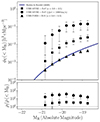 |
Fig. B.1. Rest-frame UV luminosity function for the sample of UBR color-selected LBGs. Upper panel: cumulative luminosity function of the LBGs identified within the FoV of MUSE (squares) and FORS2 (triangles), and of those galaxies with spectroscopic redshift within |Δv| ≤ 1000 km s−1 around the central QSO (points). The LBGs’ luminosity functions are corrected for the 1D completeness of the R-band that is used for the detection (see Figure 1). Lower panel: overdensity as a function of the R-band magnitude. |
Appendix C: Alignment of the LBGs with the large-scale overdensity
Assuming the LBGs span the entire redshift range 3.0 < z < 3.5 (see Section 3.1), we measured the local co-moving galaxy density by using the Nth neighbor estimator with the same formalism presented by Shimakawa et al. (2018a). We choose N = 5. Although we expect this method to not be efficient at the edges of the FoV, these galaxies should not affect the statistics significantly and are mostly limited to R ≳ 11 cMpc. Furthermore, we validate the choice of the estimator by comparing the Nth neighbor results to the co-moving density obtained by the scale independent the Voronoi Tessellation, described in Section 4.6. We observe that the 3rd neighbor systematically over-estimate the density by a factor of ≈1.5 compared to the Voronoi Tessellation, but the two methods turn out to be consistent for N ≥ 5. The local density is finally converted into a co-moving overdensity  against the expected density of galaxies in a blank field (see Section 4.2).
We then measured the orientation of each galaxy with respect to the north-south direction and the central QSO. In bins of co-moving overdensity defined to contain roughly the same number of galaxies, we measured the fraction of LBGs oriented along the north-south direction around the QSO as a function of the environment (see Figure C.1). We require a galaxy for being aligned to the north-south direction to be offset by an angle within ±25° (black, corresponding to 0° −25° or 155° −180°) or ±45° (magenta, corresponding to 0° −45° or 135° −180°), chosen so that ≳40% and 100%, respectively, of the MUSE spectroscopic sample is found to be aligned.
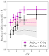 |
Fig. C.1. Fraction of LBGs aligned with respect to the north-south direction, relative to the QSO, as a function of the local overdensity. We require a galaxy to be aligned if found within ±25° (black, corresponding to 0° −25° or 155° −180°) or ±45° (magenta, corresponding to 0° −45° or 135° −180°) the north-south direction. The shaded area shows the 16th and 84th percentiles of the distribution expected for random samples of 1, 000 bootstrap realizations. |
Figure C.1 shows that the fraction of LBGs oriented along the north-south direction steeply increases with the local co-moving density. In other words, the regions that overdense in LBGs are not sparsely distributed across the large area we surveyed, but instead do preferentially follow the same orientation as the spectroscopically selected galaxies within 4 × 4 cMpc2 and Δv = ± 1000 km s−1 from the central QSO. To further support this result, we reproduce the expectations for a sample of randomly distributed galaxies by injecting the same number of LBGs of the real data in random positions across the FoV. We repeat the injection 1, 000 times and show, despite the large uncertainties derived from the 16th and 84th percentile of the bootstrap distribution, that the fraction of aligned galaxies is flat as a function of the co-moving galaxy overdensity. To support this argument on a more statistical ground, we performed a Spearman’s rank correlation test on both the data and the bootstrap results. For the data we found a positive correlation that is significant well above 2σ, as given by ρspearman = 0.93, p−value = 0.003 for the threshold ±45°, and ρspearman = 0.97, p−value = 0.0005 for ±25°. On the other hand, for the random-like samples we find ρspearman = 0.01, p−value = 0.78 for the threshold ±45°, and ρspearman = 0.02, p−value = 0.86 for ±25°. Altogether, this analysis provides a piece of strong evidence for the distribution of massive LBGs to be preferentially aligned along the direction of the overdensity of star-forming galaxies observed in a much smaller volume around the central QSO and thus further supports a picture in which the gaseous structure embedding these galaxies extends for several tens of comoving megaparsecs.
Appendix D: MQN01 clustering compared to the MAGG survey
The clustering analysis presented in Section 4.3 and discussed in Section 5.1 provides hints that the MQN01 QSO can possibly be associated to a halo that is much larger compared to those of average QSOs at similar redshifts. To further support this conclusion, we here give the details of the QSO-galaxy cross-correlation function we derived for continuum-selected galaxies clustered around the 28 QSOs included in the MAGG survey. Such galaxies have been identified by Lofthouse et al. (2020) running SEXTRACTOR (Bertin & Arnouts 1996) on the MUSE white-light images obtained for each of the 28 cubes centered on a 3.2 ≲ z ≲ 4.5 QSO (median z ≈ 3.7). This software outputs a segmentation map that is used to extract the spectra of all sources, which are finally inspected using MARZ Hinton et al. (2016) to assign a reliable spectroscopic redshift. As a final step, to produce a sample with a selection function that is as similar as possible to that of the MQN01 galaxies, we selected 20 galaxies with R-band magnitude mR ≲ 26.5 mag, high-quality spectroscopic redshift, and found within a line-of-sight separation |Δv| ≤ 1500 km s−1 from the central QSO of the respective field. We finally derived the projected QSO-galaxy cross-correlation function by using the same procedure described in Section 4.3. The results are shown in Figure D.1. We measured a cross-correlation length r0 = (3.8 ± 0.8) h−1cMpc for fixed γ = 1.5. Although the different sizes of the FoV, as well as the different selection and average redshift of the samples, make it difficult to compare this result with TS12, the fact that the cross-correlation in MAGG is ≈6 times smaller than that of MQN01 remains an important indicator of the rare and massive nature of the QSO host halo, as discussed in Section 5.1.
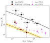 |
Fig. D.1. Projected QSO-galaxy cross-correlation functions for the continuum-selected galaxies identified in the MAGG survey (darkred and gold-shaded region). Results for the MQN01 galaxies and from TS12 are shown as in Figure 7. |
Appendix E: Results from SED fitting
We provide in this section further details and results on the galaxies’ SED fitting process. The parameters we set in the initial file of CIGALE are listed below in Table E.1, while Table E.2 shows the properties estimated for each of the 21 galaxies included in the main spectroscopic sample, as well as their redshift and results of the color-selections employed to identify the LBGs. For the sources detected in X-Ray, the derived SFR and stellar mass may be significantly affected by the contribution of the AGN emission to the total SED. We have thus investigated the morphology of these sources in the JWST/NIRCam data and verified that none of them shows compact bright emission in the center, suggesting that the contribution of the AGN emission does not outshine that of the stellar continuum. Furthermore, according to the best-fit model obtained by running CIGALE, the contribution of the AGN emission to the total galaxies’ SED is, in terms of flux density, ≳ 1 dex smaller compared to the stellar continuum. Based on these considerations, we conclude that the properties we derived for these sources are reliable and are not dominated by the presence of an AGN.
We also tested the results of the SED modeling to be independent of the code we used. To this end, we fit the observed galaxies’ photometry using the Monte Carlo Spectro-Photometric Fitter (MC-SPF, Fossati et al. 2018, 2019). The grid of stellar spectra is built upon the updated version7 of the Bruzual & Charlot (2003) high-resolution models at solar metallicity assuming an exponentially declining star formation history and the Chabrier (2003) initial mass function. A grid of nebular emission lines models from Byler et al. (2018) is scaled to the number of Lyman continuum photons from the stellar models, converted into flux at the redshift of the galaxies, and then added to templates. To model the dust attenuation, we assume the double attenuation law from Calzetti et al. (2000), which includes extra extinction of the young stars compared to those older than 10 Myr. Comparing the two SED fitting codes, the median difference we observe in the galaxies’ properties is 0.048 ± 0.050 dex for the stellar mass and 0.054 ± 0.055 dex for the SFR, which is in both the cases substantially smaller than other uncertainties associated to these parameters.
Input parameters for the SED fitting code CIGALE.
Detailed results of the galaxies’ SED fitting.
All Tables
Report of UBR and UGR color selections calibrated to identify 3.0 < z < 3.5 LBGs around the central QSO.
Results of the Spearman-rank test on the correlations between the properties of the MQN01 galaxies and the local overdensity.
All Figures
|
Fig. 1. Completeness estimated for the VLT/FORS2 images in the U (blue), B (black), and R band (red). The solid line is the result across the entire FoV, while the shaded regions reproduce the variation from the shallower to the deepest regions of each mosaic. The vertical dotted lines mark the magnitudes corresponding to the 50% completeness limit (black horizontal line). |
| In the text | |
|
Fig. 2. Visualization of the multiwavelength data explored in this work. Left panel: FORS2/R-band image with overlaid the footprint of the MUSE (purple), FORS2 and HAWK-I (orange), HST/ACS F625W (blue), HST/ACS F814W (light-blue), JWST/NIRCam (red) and ALMA/Band3 and Band6 (green) observations. Right panel: the zoom-in shows the MUSE White-Light image in the background with highlighted the MQN01 high-confidence sample of galaxies found in the MUSE FoV within a line-of-sight separation |Δv|≤1000 km s−1 around the QSO (blue squares), the cross-matched CO(4–3) line-emitters found by ALMA (green diamonds, see Pensabene et al. 2024) and X-Ray sources detected by Chandra (red circles, see Travascio et al. 2025). The target QSO is marked by a gold star. |
| In the text | |
|
Fig. 3. UBR color selection of LBGs. The selection region (delimited by solid black lines) is calibrated based on the redshift tracks of typical LBG templates (dashed lines). The orange density contours show the LBGs candidates at z ≈ 3.0 − 3.5 that are selected by our criterion. The sources with spectroscopic redshift from MUSE and found within |Δv|≤1000 km s−1 from the central QSO are shown as stars and are color-coded by their visual extinction, Av, estimated by fitting their SEDs (see Section 3.4). The gray density contours mark all the R-band detection within the FORS2 FoV. Typical errors on the colors are shown in the lower-left corner. |
| In the text | |
|
Fig. 4. Examples of source classification based on the quality of spectroscopic redshift constraints in MUSE. Left panels: spectra (black) and errors (violet) extracted from MUSE datacubes up to the rest-frame wavelength of the C IV transition (corresponding to observed 6580 Å at z = 3.25), with major spectral features highlighted by vertical dotted lines, as discussed in Section 2.1. When these features are clearly visible, the source is assigned a high-confidence redshift (upper panel). In contrast, when only the Lyα emission line is detected, the redshift measurement is considered low confidence (lower panel). Right panels: 2″ × 2″ cutouts of the MUSE white-light image used for source detection, with the sources indicated by white arrows. |
| In the text | |
|
Fig. 5. Redshift distributions of the MQN01 high-confidence spectroscopic sample (black histogram) and of the UBR-selected LBGs with secure spectroscopic redshift from MUSE (hatched gray histogram). These are compared to the “MUSE-FIELD” sample and normalized by the surveyed area. The redshift of the central QSO is marked by an orange vertical line. The inset shows the velocity distribution of the MUSE galaxies and of the LBGs relative to the redshift of the QSO. The line-of-sight velocity window corresponding to |Δv|≤1000 km s−1 is highlighted by dotted vertical lines. |
| In the text | |
|
Fig. 6. Luminosity functions and overdensity of galaxies identified around the central QSO. Upper panel: cumulative R-band luminosity function of the MQN01 galaxies found within |Δv|≤1000 km s−1 from the redshift of the QSO (black stars), compared to that of the “MUSE-FIELD” sample (black pentagons) and of the control sample of sources found in the MQN01 MUSE FoV within 2.5 < z < 4.5, masking |Δv|≤1500 km s−1 around the QSO (orange diamonds). The vertical dotted line shows the magnitude at which the luminosity function of the spectroscopic samples flattens relative to the completeness-corrected one from Reddy & Steidel (2009). Lower panel: overdensity as a function of the R-band magnitude. |
| In the text | |
|
Fig. 7. Projected correlation functions assuming fixed γ = 1.8 and linking window |Δv|≤1000 km s−1. The QSO-galaxy cross-correlation function for the MUSE spectroscopic sample (black stars) is similar to that of CO(4–3) line emitters identified by Pensabene et al. (2024) in the same volume (blue line and shaded area), but significantly above that of Trainor & Steidel (2012) (purple, filled points). The galaxy-galaxy auto-correlation function is shown for the control-field sample of z = 2.5 − 4.5 galaxies identified in the UDF (black pentagons, Bacon et al. 2023), together with upper limits for the galaxies in our field within the same redshift range, but masking |Δv|≤1500 km s−1 around the redshift of the QSO (orange diamonds). Both the estimates are consistent with Trainor & Steidel (2012) (purple, empty points). The best-fit results are shown as dotted and solid lines for the auto and cross-correlation functions, respectively. All the uncertainties are derived from the 16th and 84th percentiles from bootstrap distributions. |
| In the text | |
|
Fig. 8. Star-forming main sequence, in terms of SFR (left panel) and sSFR (right panel), of the MQN01 galaxies clustered around the QSO (black stars), compared to the control-field sample (orange diamonds). The data are compared to the main sequence at z ≈ 3.25 derived from Speagle et al. (2014) (blue), Popesso et al. (2023) (green) and Koprowski et al. (2024) (purple). The X-Ray detected AGN are marked by yellow squares. The histograms on the top and right panels show the distribution of the SFR or sSFR and galaxies’ stellar mass, respectively, of the MQN01 galaxies (black) and of the control-field sample, together with their median values on top. |
| In the text | |
|
Fig. 9. Excess of massive log(M⋆/M⊙)≳10.5 galaxies around the MQN01 QSO. Left panel: cumulative stellar mass function of the MQN01 spectroscopic sample in proximity to the QSO (black stars) compared to the control-field sample (orange diamonds) and the expectations for blank fields from the COSMOS survey (3.0 < z < 3.5, Weaver et al. 2023, gray). Right panel: same as the left panel, but normalized to the value of the cumulative mass function at M⋆ = 109.8 M⊙, corresponding to the 90% completeness limit of the MQN01 spectroscopic sample. |
| In the text | |
|
Fig. 10. MQN01 galaxies’ SFR (1st panel), stellar mass (2nd panel) and sSFR (3rd panel) as a function of the co-moving local galaxy density (bottom x-axis) and overdensity (top x-axis) with respect to the field. X-Ray emitting AGN detected in Chandra observations are highlighted as yellow squares. |
| In the text | |
|
Fig. 11. 2D overdensity maps of the LBGs and of the spectroscopically selected galaxies found to be clustered with the QSO. Left panel: Overdensity map of the LBGs identified within the 24 × 24 cMpc2 FORS2 FoV. The amplitude of the overdensity is shown in shades of blue scaling with the colormap. Contours are shown for |
| In the text | |
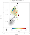 |
Fig. A.1. Same as Figure 3, but showing the results of the UGR color selection of LBGs. |
| In the text | |
|
Fig. B.1. Rest-frame UV luminosity function for the sample of UBR color-selected LBGs. Upper panel: cumulative luminosity function of the LBGs identified within the FoV of MUSE (squares) and FORS2 (triangles), and of those galaxies with spectroscopic redshift within |Δv| ≤ 1000 km s−1 around the central QSO (points). The LBGs’ luminosity functions are corrected for the 1D completeness of the R-band that is used for the detection (see Figure 1). Lower panel: overdensity as a function of the R-band magnitude. |
| In the text | |
|
Fig. C.1. Fraction of LBGs aligned with respect to the north-south direction, relative to the QSO, as a function of the local overdensity. We require a galaxy to be aligned if found within ±25° (black, corresponding to 0° −25° or 155° −180°) or ±45° (magenta, corresponding to 0° −45° or 135° −180°) the north-south direction. The shaded area shows the 16th and 84th percentiles of the distribution expected for random samples of 1, 000 bootstrap realizations. |
| In the text | |
|
Fig. D.1. Projected QSO-galaxy cross-correlation functions for the continuum-selected galaxies identified in the MAGG survey (darkred and gold-shaded region). Results for the MQN01 galaxies and from TS12 are shown as in Figure 7. |
| In the text | |
Current usage metrics show cumulative count of Article Views (full-text article views including HTML views, PDF and ePub downloads, according to the available data) and Abstracts Views on Vision4Press platform.
Data correspond to usage on the plateform after 2015. The current usage metrics is available 48-96 hours after online publication and is updated daily on week days.
Initial download of the metrics may take a while.