| Issue |
A&A
Volume 683, March 2024
|
|
|---|---|---|
| Article Number | A223 | |
| Number of page(s) | 47 | |
| Section | Extragalactic astronomy | |
| DOI | https://doi.org/10.1051/0004-6361/202346855 | |
| Published online | 21 March 2024 | |
1100 days in the life of the supernova 2018ibb
The best pair-instability supernova candidate, to date⋆
1
The Oskar Klein Centre, Department of Physics, Stockholm University, Albanova University Center, 106 91 Stockholm, Sweden
e-mail: This email address is being protected from spambots. You need JavaScript enabled to view it.
2
The Oskar Klein Centre, Department of Astronomy, Stockholm University, Albanova University Center, 106 91 Stockholm, Sweden
3
Heidelberger Institut für Theoretische Studien, Schloss-Wolfsbrunnenweg 35, 69118 Heidelberg, Germany
4
Technische Universität München, TUM School of Natural Sciences, Physik-Department, James-Franck-Straße 1, 85748 Garching, Germany
5
Max-Planck-Institut für Astrophysik, Karl-Schwarzschild Straße 1, 85748 Garching, Germany
6
Max-Planck-Institut für Extraterrestrische Physik, Giessenbachstraße 1, 85748 Garching, Germany
7
Department of Particle Physics and Astrophysics, Weizmann Institute of Science, 234 Herzl St, 76100 Rehovot, Israel
8
The Caltech Optical Observatories, California Institute of Technology, Pasadena, CA 91125, USA
9
Finnish Centre for Astronomy with ESO (FINCA), 20014 University of Turku, Turku, Finland
10
Tuorla Observatory, Department of Physics and Astronomy, University of Turku, 20014 Turku, Finland
11
DTU Space, National Space Institute, Technical University of Denmark, Elektrovej 327, 2800 Kgs. Lyngby, Denmark
12
Department of Physics, University of Oxford, Denys Wilkinson Building, Keble Road, Oxford OX1 3RH, UK
13
Astrophysics Research Centre, School of Mathematics and Physics, Queen’s University Belfast, Belfast BT7 1NN, UK
14
Department of Astronomy, University of California, Berkeley, CA 94720-3411, USA
15
Birmingham Institute for Gravitational Wave Astronomy and School of Physics and Astronomy, University of Birmingham, Birmingham B15 2TT, UK
16
Nordita, Stockholm University and KTH Royal Institute of Technology Hannes Alfvéns väg 12, 106 91 Stockholm, Sweden
17
Division of Physics, Mathematics and Astronomy, California Institute of Technology, Pasadena, CA 91125, USA
18
INAF – Osservatorio di Astrofisica e Scienza dello Spazio, Via Piero Gobetti 93/3, 40129 Bologna, Italy
19
Physics Department and Tsinghua Center for Astrophysics (THCA), Tsinghua University, Beijing 100084, PR China
20
Gemini Observatory/NSF’s NOIRLab, Casilla 603, La Serena, Chile
21
MIT-Kavli Institute for Astrophysics and Space Research, 77 Massachusetts Ave., Cambridge, MA 02139, USA
22
Department of Astrophysics, University of Vienna, Türkenschanzstraße 17, 1180 Vienna, Austria
23
Cosmic Dawn Center (DAWN), Denmark; Niels Bohr Institute, Copenhagen University, Jagtvej 128, 2200 Copenhagen N, Denmark
24
Department of Astronomy, Cornell University, Ithaca, NY 14853, USA
25
Cardiff Hub for Astrophysics Research and Technology, School of Physics & Astronomy, Cardiff University, Queens Buildings, The Parade, Cardiff CF24 3AA, UK
26
Tuorla Observatory, Department of Physics and Astronomy, University of Turku, 20014 Turku, Finland
27
Finnish Centre for Astronomy with ESO (FINCA), University of Turku, 20014 Turku, Finland
28
Astrophysics Research Institute, Liverpool John Moores University, Liverpool Science Park, 146 Brownlow Hill, Liverpool L3 5RF, UK
29
Large Binocular Telescope Observatory, University of Arizona, 933 N. Cherry Ave., Tucson, AZ 85721, USA
30
George Mason University, Department of Physics & Astronomy, MS 3F3, 4400 University Dr., Fairfax, VA 22030, USA
31
GSI Helmholtzzentrum für Schwerionenforschung, Planckstraße 1, 64291 Darmstadt, Germany
32
Department of Astronomy and Astrophysics, University of California, Santa Cruz, CA 95064, USA
33
INAF – Osservatorio Astronomico di Padova, vicolo dell’Osservatorio 5, 35122 Padova, Italy
34
INAF – Osservatorio Astronomico d’Abruzzo, Via M. Maggini snc, 64100 Teramo, Italy
35
European Southern Observatory, Alonso de Córdova 3107, Casilla 19, Santiago, Chile
36
Millennium Institute of Astrophysics MAS, Nuncio Monsenor Sotero Sanz 100, Off. 104, Providencia, Santiago, Chile
37
INAF – Istituto di Astrofisica Spaziale e Fisica cosmica Milano (IASF), Via Alfonso Corti 12, 20133 Milano, Italy
38
Institute of Space Sciences (ICE, CSIC), Campus UAB, Carrer de Can Magrans, s/n, 08193 Barcelona, Spain
39
Institut d’Estudis Espacials de Catalunya (IEEC), 08034 Barcelona, Spain
40
Astronomical Observatory, University of Warsaw, Al. Ujazdowskie 4, 00-478 Warszawa, Poland
41
IPAC, California Institute of Technology, 1200 E. California Blvd, Pasadena, CA 91125, USA
42
Center for Astrophysics, Harvard & Smithsonian, 60 Garden Street, Cambridge, MA 02138-1516, USA
43
Las Cumbres Observatory, 6740 Cortona Dr. Suite 102, Goleta, CA 93117, USA
44
Department of Physics, University of California, Santa Barbara, CA 93106-9530, USA
45
Department of Physics, University of California, 1 Shields Avenue, Davis, CA 95616-5270, USA
46
Université de Lyon, Université Claude-Bernard Lyon 1, CNRS/IN2P3, IP2I Lyon, 69622 Villeurbanne, France
47
Lunar and Planetary Laboratory, University of Arizona, Tucson, AZ 85721, USA
48
The NSF AI Institute for Artificial Intelligence and Fundamental Interactions, Cambridge, USA
Received:
9
May
2023
Accepted:
11
October
2023
Abstract
Stars with zero-age main sequence masses between 140 and 260 M⊙ are thought to explode as pair-instability supernovae (PISNe). During their thermonuclear runaway, PISNe can produce up to several tens of solar masses of radioactive nickel, resulting in luminous transients similar to some superluminous supernovae (SLSNe). Yet, no unambiguous PISN has been discovered so far. SN 2018ibb is a hydrogen-poor SLSN at z = 0.166 that evolves extremely slowly compared to the hundreds of known SLSNe. Between mid 2018 and early 2022, we monitored its photometric and spectroscopic evolution from the UV to the near-infrared (NIR) with 2–10 m class telescopes. SN 2018ibb radiated > 3 × 1051 erg during its evolution, and its bolometric light curve reached > 2 × 1044 erg s−1 at its peak. The long-lasting rise of > 93 rest-frame days implies a long diffusion time, which requires a very high total ejected mass. The PISN mechanism naturally provides both the energy source (56Ni) and the long diffusion time. Theoretical models of PISNe make clear predictions as to their photometric and spectroscopic properties. SN 2018ibb complies with most tests on the light curves, nebular spectra and host galaxy, and potentially all tests with the interpretation we propose. Both the light curve and the spectra require 25–44 M⊙ of freshly nucleosynthesised 56Ni, pointing to the explosion of a metal-poor star with a helium core mass of 120–130 M⊙ at the time of death. This interpretation is also supported by the tentative detection of [Co II] λ 1.025 μm, which has never been observed in any other PISN candidate or SLSN before. We observe a significant excess in the blue part of the optical spectrum during the nebular phase, which is in tension with predictions of existing PISN models. However, we have compelling observational evidence for an eruptive mass-loss episode of the progenitor of SN 2018ibb shortly before the explosion, and our dataset reveals that the interaction of the SN ejecta with this oxygen-rich circumstellar material contributed to the observed emission. That may explain this specific discrepancy with PISN models. Powering by a central engine, such as a magnetar or a black hole, can be excluded with high confidence. This makes SN 2018ibb by far the best candidate for being a PISN, to date.
Key words: supernovae: individual: SN 2018ibb / supernovae: individual: ATLAS18unu / supernovae: individual: Gaia19cvo / supernovae: individual: PS19crg / supernovae: individual: ZTF18acenqto
Tables 1 and C.1 and SN 2018ibb: multi-band and bolometric light curves, and blackbody properties are available at the CDS via anonymous ftp to cdsarc.cds.unistra.fr (130.79.128.5) or via https://cdsarc.cds.unistra.fr/viz-bin/cat/J/A+A/683/A223
NASA Einstein Fellow.
© The Authors 2024
 Open Access article, published by EDP Sciences, under the terms of the Creative Commons Attribution License (https://creativecommons.org/licenses/by/4.0), which permits unrestricted use, distribution, and reproduction in any medium, provided the original work is properly cited.
This article is published in open access under the Subscribe to Open model. This email address is being protected from spambots. You need JavaScript enabled to view it. to support open access publication.
1. Introduction
Observations of stellar nurseries (e.g. Krumholz et al. 2019), as well as massive stars (e.g. Crowther 2007) and their fates (e.g. Filippenko 1997; Gal-Yam 2017) have led to stellar evolution models of an ever-increasing complexity (e.g. McKee & Ostriker 2007). These models also predict the existence of stars with ≳100 M⊙ (e.g. Heger & Woosley 2002; Heger et al. 2003), which may have no analogues in the local Universe (Mackey et al. 2003; Bromm & Larson 2004; Langer et al. 2007, but see Brands et al. 2022), and exotic types of stellar explosions (Fowler & Hoyle 1964; Rakavy et al. 1967; Woosley et al. 2007; Sakstein et al. 2022).
One of those predicted, yet not securely discovered object classes, is pair-instability supernovae (PISNe). This SN class is produced by the thermonuclear runaway of metal-poor stars with zero-age main sequence (ZAMS) masses between 140 and 260 M⊙ (Fowler & Hoyle 1964; Barkat et al. 1967; Rakavy et al. 1967). When such a massive star dies, its helium core would have grown to 65–130 M⊙ (Heger & Woosley 2002). The combination of a relatively low matter density and high temperature leads to the production of e−e+ pairs, reducing the radiation pressure that supports the star against the gravitational collapse. As a result, implosive oxygen and silicon burning produce enough energy to revert the collapse and obliterate the entire star, leaving no remnant behind.
During the past 15 yr, PISNe have been a focus of fundamental physics and SN science. Stars with helium-topped cores slightly less massive than ∼65 M⊙ presumably leave black holes behind, and stars whose helium-topped cores exceed ∼130 M⊙ are thought to collapse directly into black holes. In this paradigm, there should be a dearth of black holes with masses between ∼50 and ∼120 M⊙ (Farmer et al. 2019; Renzo et al. 2020). Observations by the Laser Interferometer Gravitational-Wave Observatory (LIGO) and the Virgo interferometer found tentative evidence for the existence of such a drop in the black-hole mass function (The LIGO Scientific Collaboration 2021). A more recent study by the LIGO–Virgo collaboration using the larger Gravitational-Wave Transient Catalog 3 shows that the evidence of a mass gap at ∼50 M⊙ is inconclusive (The LIGO Scientific Collaboration 2023). However, this could be due to the inclusion of binary black holes that formed through dynamical channels involving repeated mergers rather than evidence for the lack of a mass gap (e.g. Belczynski et al. 2020; Gerosa & Fishbach 2021, and references therein). A further consequence of the PISN model is its peculiar nucleosynthetic pattern. In the case of an extremely metal-poor star being formed from the gas of PISN ejecta, its chemical composition should show a strong variance between elements with an odd and even nuclear charge (Heger & Woosley 2002; Umeda & Nomoto 2002). Xing et al. (2023) recently reported the discovery of a very metal-poor star with such a chemical signature (for additional candidates see also Aoki et al. 2014; Salvadori et al. 2019), lending support to the first stars having been very massive and exploding as PISNe.
Finding PISNe is one of the main challenges in the SN field. PISN models predict that up to ∼57 M⊙ of radioactive 56Ni are produced during the thermonuclear runaway (Heger & Woosley 2002). Such high Ni-yield PISNe are thought to produce long-lived (rise times > 80 days), luminous (Mpeak < −21 mag) transients (Kasen et al. 2011; Kozyreva et al. 2017) in the regime of superluminous supernovae (SLSNe; Quimby et al. 2011; Gal-Yam 2012, 2019a). Although the powering mechanism of SLSNe is debated (Gal-Yam et al. 2009; Blinnikov & Sorokina 2010; Inserra et al. 2013), numerous studies of both H-poor and H-rich SLSNe have revealed that nickel is not the primary source of energy (e.g. Chatzopoulos & Wheeler 2012; Chen et al. 2013, 2023a; Inserra et al. 2013, 2018; Nicholl et al. 2017; Moriya et al. 2018a; Gal-Yam 2019a; Inserra 2019; Kangas et al. 2022). Yet, a few SLSNe had markedly broad and luminous light curves similar to predictions of PISN models, for example, SN 1999as, SN 2007bi, PTF12dam, PS1-14bj, and SN 2015bn (Hatano et al. 2001; Gal-Yam et al. 2009; Nicholl et al. 2013, 2016a; Chen et al. 2015; Lunnan et al. 2016; Kozyreva et al. 2017). However, the published candidates either had incomplete datasets, not long enough rise times, too high ejecta velocities, too blue spectra, or exploded in galaxies with a metallicity that is too high to conclusively argue for the discovery of a PISN (e.g. Nicholl et al. 2013; Jerkstrand et al. 2017).
Not all PISNe are expected to be superluminous. The stars at the low-mass end of the PISN range (M(ZAMS)≳140 M⊙ equivalent to a He-core mass of ≳65 M⊙ at the end of their evolution) are thought to produce a small-to-no-mass of 56Ni (Kasen et al. 2011; Kozyreva et al. 2014; Gilmer et al. 2017). The bright supernova OGLE-2014-SN-073 is a candidate for a low-mass PISN, as its light curve would require only ∼1 M⊙ of 56Ni (Terreran et al. 2017; Kozyreva et al. 2018, but see also Dessart & Audit 2018 and Moriya et al. 2018b for alternative interpretations). However, also in that case, there is still some tension between observations and theoretical models due to the unknown explosion date and the lack of sufficiently early data to search for the luminous shock-breakout predicted by PISN models (Kozyreva et al. 2018). The Type I SN 2016iet is another candidate for a lower-mass PISN. Gomez et al. (2019) concluded that the light curve could be powered by a few M⊙ of 56Ni. However, the SN was discovered only around maximum light. Furthermore, its nebular spectra are very different to the PISN model spectra from Mazzali et al. (2019) as pointed out by Gomez et al. (2019). While the inferred nickel mass of a few M⊙ and ejecta mass of ∼64 M⊙ could point to a PISN explosion, other powering mechanisms are also possible (Gomez et al. 2019).
In June 2018, the Zwicky Transient Facility (ZTF; Bellm et al. 2019a; Graham et al. 2019) started to survey the northern sky every 2–3 nights in two filters and detects thousands of supernovae every year (Fremling et al. 2020; Perley et al. 2020). Until autumn 2021, we carried out a systematic survey for SLSNe in ZTF (Chen et al. 2023a,b). SN 2018ibb, the slowest evolving SLSN in our sample, has several properties that match predictions of PISN models. Between mid 2018 and early 2022, we built a comprehensive photometric and spectroscopic dataset covering the evolution from tmax–93 to tmax+1000 rest-frame days to scrutinise SLSN and PISN models. In this paper, we present this dataset along with our conclusions on SN 2018ibb’s source of energy and progenitor. The paper is structured as follows: we report the SN discovery in Sect. 2 and describe the observations in Sect. 3. In Sect. 4, we derive the properties of SN 2018ibb’s light curve, spectra and host galaxy and in Sect. 5 we contrast SLSN and PISN models with our dataset. Finally, in Sect. 6 we summarise our findings and present our conclusions on the nature of SN 2018ibb and its connection to PISNe.
Throughout the paper, we provide all uncertainties at 1σ confidence. The photometry is reported in the AB system. We assume ΛCDM cosmology with H0 = 67.8 km s−1 Mpc−1, ΩM = 0.308, and ΩΛ = 0.692 (Planck Collaboration XIII 2016). Phase information is reported in the rest-frame with respect to the g|r-band maximum (tmax) at MJD = 58455.
2. Discovery
SN 2018ibb, located at α = 04:38:56.950, δ = –20:39:44.10 (J2000), was discovered by the Asteroid Terrestrial-impact Last Alert System (ATLAS; Tonry 2011; Smith et al. 2020) survey as ATLAS18unu on 10 September 2018 with an apparent magnitude of o = 18.89 mag (wavelength range 5600–8200 Å; Tonry et al. 2018). Later detections were reported by the public northern sky survey of the Zwicky Transient Facility (Bellm et al. 2019b) on 16 November 2018 (internal name: ZTF18acenqto), the Pan-STARRS Survey for Transients (Huber et al. 2015) on 8 January 2019 (internal name: PS19crg) and the Gaia Photometric Science Alerts transient survey (Hodgkin et al. 2021) on 4 July 2019 (internal name: Gaia19cvo). A false-colour image of the field when SN 2018ibb was bright and after it had faded is shown in Fig. 1. Fremling et al. (2018a) initially classified SN 2018ibb as a Type Ia SN on 5 December 2018 but retracted this classification on 6 December 2018 and set a new classification to “supernova” on 6 December 2018 (Fremling et al. 2018b). Pursiainen et al. (2018) obtained a spectrum with the 3.58 m New Technology Telescope at La Silla Observatory (Chile) as a part of the Extended Public ESO Spectroscopic Survey of Transient Objects (ePESSTO; Smartt et al. 2015) on 14 December 2018 and classified SN 2018ibb as a H-poor SLSN at z = 0.16.
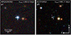 |
Fig. 1. False-colour image of the field when SN 2018ibb was bright (left) and after it had faded below the host level (right). The SN position, marked by the crosshair, is located ∼1 kpc from the centre of its star-forming dwarf host galaxy ( |
3. Observations and data reduction
3.1. Supernova photometry
Our imaging campaign had three tiers: (i) all-sky surveys with sufficient depth and cadence to monitor the evolution from tmax–93 to tmax+306 days; (ii) dedicated follow-up campaigns to expand the wavelength coverage to the UV and near-IR and to extend the light curve coverage to tmax+1000 days; and (iii) smaller targeted campaigns to mitigate data gaps, expand the wavelength coverage to the near-IR, and ensure a good flux calibration of the photometric and spectroscopic data. Owing to the large number of facilities involved in this effort, we present the details of each campaign and the data reduction in Appendix A.
The ground-based photometry was calibrated with field stars from PanSTARRS1 (Chambers et al. 2016, PS1), the Dark Energy Survey (DES; The Dark Energy Survey Collaboration 2005), the Dark Energy Spectroscopic Instrument (DESI) Legacy Imaging survey (LS; Dey et al. 2019), and the Two Micron All-Sky Survey (2MASS; Skrutskie et al. 2006). We applied known colour equations between PS1/DES and Bessell/GROND/SDSS/ZTF filters (Finkbeiner et al. 2016; Drlica-Wagner et al. 2018; Greiner et al. 2008; Medford et al. 2020) and Lupton1, to account for differences in the filter response function. We applied the offsets from Blanton & Roweis (2007) to convert all measurements to the AB photometric system. The Swift/UVOT data were calibrated with zeropoints from the Swift pipeline and converted to the AB system following Breeveld et al. (2011). The HST photometry was done with a custom-made aperture photometry tool, based on the python package PHOTUTILS (Bradley et al. 2020) version 1.5, using an aperture with a diameter of 0 5 and calibrated against tabulated zeropoints in PYSYNPHOT version 2.0.0 (STScI Development Team 2013).
SN spectra are characterised by strong absorption and emission features that evolve with time. This can lead to time-dependent colour terms between similar but not identical filters (e.g. Stritzinger et al. 2002) and add a non-negligible systematic scatter to the light curves if these differences are not corrected. To illustrate this issue, we compute the synthetic magnitude in ZTF/g, GROND/g and EFOSC2/g at tmax and tmax+210 days2. At tmax, the colour term between the EFOSC2/GROND and ZTF filters is −0.01 and +0.04 mag, respectively, but at tmax+210 days the differences increased to −0.13 and +0.12 mag. Since the EFOSC2 and GROND data cover the late-time evolution, the differences in the filters would be well visible in the final light curve if they remained uncorrected.
To calibrate the various datasets into the same photometric system, we defined a set of reference filters consisting of the Swift filters, ZTF/gr, GROND/izJH and 2MASS/K. Then, we extracted synthetic photometry of all ground-based filters used in our campaign from the Keck and VLT spectra (Sect. 3.3), which were obtained in clear/photometric conditions, and measured the expected colours with respect to our reference filter system as a function of time. After applying this s-correction (Stritzinger et al. 2002), we merged the different datasets to build a photometric sequence of SN 2018ibb from tmax–93 to tmax+706 days. We omitted these corrections for the BVJHK data because most observations in these filters were done with the same instrument. We also skipped applying an s-correction on the HST observations in F336W at tmax+1645 days as the SN was not detected anymore. Table A.1 summarises the homogenised SN photometry. The measurements are not corrected for Galactic extinction along the line of sight [E(B − V)=0.03 mag; Schlafly & Finkbeiner 2011], but this correction is applied to all derived properties and photometric data presented in this paper.
The photometry is available on WISeREP3 (Yaron & Gal-Yam 2012). It is also available as a machine-readable table in the electronic version of this paper.
3.2. Host galaxy photometry
We obtained additional photometry with the ESO VLT, the 3.58 m New Technology Telescope and the Hubble Space Telescope approximately 1000 days after maximum (Appendix A). The brightness of the host galaxy was measured with elliptical apertures encircling the entire host galaxy and calibrated in the same way as the SN photometry. The HST photometry was done with a custom-made aperture photometry tool, based on the python package PHOTUTILS, using an aperture comparable in area to the ground-based images and calibrated against tabulated zeropoints in PYSYNPHOT. In the R-band, we measure a brightness of 24.39 ± 0.05 mag. The brightness in the other filters is reported in Table 1.
Photometry of the host galaxy.
Log of spectroscopic observations.
3.3. Spectroscopy
We collected a series of spectra spanning from the time of maximum to tmax+989.2 days. Similarly to the imaging campaign, we utilised a large number of 2–10 m class telescopes. A brief summary of the observations is provided in Table 2. The details of the observations and data reduction are presented in Appendix B. All spectra were absolute-flux-calibrated with multi-band photometry. Since the photometry was not obtained contemporaneously with the spectroscopic observation, we linearly interpolated between adjacent observations.
The spectra obtained after August 2021 have an increasing contribution from the host galaxy. The host contamination was removed with the FORS2 spectrum from January 2022 (tmax+989.2 days). The slit did not cover the entire host galaxy. We scaled the spectrum to the flux encircled by the slit. We note that to determine whether SN 2018ibb contributed to the observed spectrum from January 2022, we compared the observed spectrum to the fit of the spectral energy distribution (SED) of the entire host galaxy. The continuum level of the January 2022 spectrum is fully consistent with the best fit to the host galaxy SED (Fig. D.1). The only remaining SN feature is broad [O III] λλ 4959,5007 in emission, produced by the interaction of the SN ejecta with circumstellar material (Sect. 5.1). Owing to that, we masked the region and estimated the host galaxy flux with linear interpolation. To recover the host-subtracted spectrum of SN 2018ibb from the January 2022 epoch, we utilised the best fit to the galaxy SED.
All data were also corrected for Milky-Way (MW) extinction. We note that a few spectra were affected by adverse weather conditions. The absolute-flux calibrated spectra without MW extinction correction are available on WISeREP.
3.4. Imaging polarimetry
To measure the ejecta geometry, we acquired four epochs of imaging polarimetry in the v_HIGH filter with VLT/FORS2 between tmax+31.9 and tmax+94.4 days (Table 3). In addition, we got one epoch with the R_SPECIAL filter at tmax+94.4 days. Each polarisation measurement required four exposures at four different retarder-plate angles: 0°,  , 45°, and
  . The beam was split with a Wollaston prism into the ordinary (o) and the extraordinary (e) ray. The o-ray and the e-ray were placed at the 7th and the 8th multi-object spectroscopy (MOS) stripes, respectively.
Log of polarimetric observations.
We reduced the data in a standard manner using IRAF (Tody 1993) tasks. The flux of the SN in the o-ray and e-ray were measured through aperture photometry at all four retarder-plate angles using the DAOPHOT.PHOT package (Stetson 1987). Stokes parameters and polarisation of the target were derived based on the FORS2 manual (Anderson et al. 2018), and the polarisation degrees were corrected for polarisation bias, caused by the non-negativity nature of the polarisation degree, following Wang et al. (1997). The extracted, debiased polarisation properties are summarised in Table 3.
These values need to be corrected for polarisation induced by dichroic extinction from non-spherical dust grains that aligned with the magnetic field of the interstellar medium of the Milky Way (MW) and the host galaxy. Following Serkowski et al. (1975), the polarisation level from the Milky Way can be as high as ≲9%×E(B − V). With a Galactic extinction of E(B − V)=0.03 mag towards SN 2018ibb, the MW polarisation level could be up to 0.26%. The determination of the interstellar polarisation from SN 2018ibb’s host galaxy is not feasible. We note that the polarisation degree is only p≲0.3% in v_HIGH between tmax+32 and tmax+94 days (see Table 3). Such a low level of polarisation is very unlikely to be caused by a high intrinsic polarisation aligned and cancelled to a comparable level of significant interstellar polarisation. Therefore, without correcting for the polarisation from the host galaxy, the observations point to a high degree of spherical symmetry of SN 2018ibb during the phase of our polarisation measurement.
3.5. X-ray observations
3.5.1. Swift/XRT
While monitoring SN 2018ibb with UVOT between tmax+8.4 and tmax+224 days, Swift also observed the field with the X-ray telescope XRT between 0.3 and 10 keV in photon-counting mode (Burrows et al. 2005). We analysed these data with the online-tools of the UK Swift team4 that use the software package HEASOFT version 6.26.1 and methods described in Evans et al. (2007, 2009).
SN 2018ibb evaded detection in all epochs. The median 3σ count-rate limit of all observing blocks is 0.005 ct s−1 (0.3–10 keV). Using the dynamic rebinning option in the Swift online tools pushes the 3σ count-rate limits to 0.002 ct s−1 (median value). A list of the limits from the stacking analysis is shown in Table 4. To convert the count-rate limits into a flux, we used WEBPIMMS5 and assumed a power-law spectrum with a photon index6 of Γ = 2 and a Galactic neutral hydrogen column density of 1.97 × 1020 cm−2 (HI4PI Collaboration 2016). The average energy conversion factor for the unabsorbed flux is 3.66 × 10⁻¹¹ (erg s−1 cm−2)/(ct s−1). The median count-rate limit corresponds to an unabsorbed flux of < 7.4 × 10⁻¹⁴ erg cm−2 s−1 between 0.3–10 keV and a luminosity of < 4.9 × 1042 erg s−1. The flux and luminosity limits of the individual bins are shown in Table 4.
Log of X-ray observations.
3.5.2. XMM-Newton
The field of SN 2018ibb was also observed by XMM-Newton (Jansen et al. 2001, Principal Investigator: R. Margutti, University of California, Berkeley, USA). Four epochs were taken with the European Photon Imaging Camera (EPIC) with the pn (Strüder et al. 2001) and MOS1|2 cameras (Turner et al. 2001) between 28 January 2019 and 28 August 2019 (tmax+48.5 – tmax+230.4). We reduced the XMM-Newton/EPIC pn data using the XMM-Newton Science Analysis System7 (SAS) following standard procedures. We extracted the source using a circular region with a radius of 32″, and the background from a source-free region on the same CCD. The MOS data are shallower than the pn data, so we omit reporting them in this paper.
All XMM-Newton observations led to non-detections with count rate limits between 0.009 and 0.020 ct s−1 between 0.3 and 10 keV. Using the same spectral model as for XRT and an energy conversion factor of 1.88 × 10⁻¹² (erg s−1 cm−2)/(ct s−1), these limits translate to unabsorbed flux limits between 1.6 and 3.7 × 10⁻¹⁴ erg cm−2 s−1. Table 4 summarises the measurements.
3.6. Radio observations
The field was observed by the VLA Sky Survey (Lacy et al. 2020) between 2 and 4 GHz on 27 October 2020 (tmax+595 days). No source was detected. The flux at the SN position is −47 ± 223 μJy, translating to a 3σ flux limit of 622 μJy and a luminosity of 2 × 1039 erg s−1. Eftekhari et al. (2021) presented sub-mm observations at 100 GHz obtained with the Atacama Large Millimeter Array on 24 December 2019 (tmax+331 days). These authors also reported a non-detection with an r.m.s. of 19 μJy, translating to a 3σ flux limit of 58 μJy and a luminosity of 5 × 1039 erg s−1.
4. Results
4.1. Redshift
The X-shooter spectra between tmax+32.7 and tmax+94.3 days show narrow absorption lines of Mg Iλ 2852 and Mg IIλλ 2796,2803 from the host galaxy at a common redshift of z = 0.1660 (Fig. 2, top panel). The low-resolution FORS2 spectrum obtained at tmax+565.3 days, shown in the bottom panel of Fig. 2, reveals narrow emission lines from hydrogen and oxygen from the H II regions in the host galaxy at the same redshift as the absorption-line redshift. This redshift translates to a luminosity distance of 822.6 Mpc using the cosmological parameters from Planck Collaboration XIII (2016).
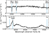 |
Fig. 2. Galaxy absorption and emission lines at a common redshift of z = 0.166 in the supernova spectra at tmax+32.7 days (top) and at tmax+565.3 days (bottom). The error spectrum of each epoch is shown in grey. |
4.2. Light curve
4.2.1. General properties
Figure 3 shows the evolution of SN 2018ibb from tmax–93 to tmax+706 rest-frame days. The early-time evolution was captured by the ATLAS, Gaia and ZTF surveys. Human scanners discovered SN 2018ibb shortly before maximum light, which triggered our large monitoring campaign from UV to NIR wavelengths. The g, r and o band light curves cover the evolution from early to late times. We use these datasets to infer the time of maximum light and the rise and decline time scales. Fitting the light curves with 3rd order polynomials between MJD = 58425 and MJD = 58485 returns the time of maximum light at MJD = 58458 ± 2, 58454 ± 2 and 58452 ± 4 in g, r and o, respectively. Throughout the paper, we adopt the weighted mean MJD 58455 ± 2 as the time of maximum light. At the time of peak, SN 2018ibb reached a brightness of 17.54 ± 0.02, 17.65 ± 0.01 and 17.92 ± 0.04 in g, r and o band, respectively (all corrected for MW extinction; Table 5)8. Using the Keck spectrum at tmax–1.4 days, we infer k-corrected absolute magnitudes of −21.79 ± 0.02, −21.66 ± 0.01 and −21.43 ± 0.04 mag in the aforementioned bands (Table 5) and a k-corrected g − r colour of −0.12 ± 0.02 mag at peak (corrected for MW extinction), a typical luminosity and colour for a H-poor SLSN (Nicholl et al. 2015a; De Cia et al. 2018; Lunnan et al. 2018a; Angus et al. 2019; Chen et al. 2023b).
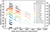 |
Fig. 3. Multi-band light curve of SN 2018ibb from 1800 to 18 500 Å (rest-frame) after correcting for the Galactic extinction. SN 2018ibb was first detected by Gaia. The last non-detections before the first detection by Gaia and ATLAS are shown by the downward-pointing triangles. With a rise time of > 93 rest-frame days, SN 2018ibb is one of the slowest evolving SLSN known. The decline of 1.1 mag (100 days)−1 is similar to the decay time of radioactive 56Co. After tmax+575 days, the decline steepened to 1.5 mag (100 days)−1. The light curve shows undulations up to tmax+100 days and a longer-lasting bump at ∼300 rest-frame days. Vertical bars represent the epochs of spectroscopy and imaging polarimetry. The absolute magnitude is computed with M = m − DM(z)+2.5 log(1+z), where DM is the distance modulus and z the redshift. |
Light curve properties.
Similar to Chen et al. (2023b), we measure the rise and decline time scales from 10% and 50% peak flux to peak in all three bands. In the g band, we obtain t1/2, rise = 52 ± 1 days,  days, t1/10, rise > 79.3 days, and t1/10, decline = 242 ± 1 days, that is, 1 mag (100 days)−1 (all measured in the rest-frame). The light curve parameters in the other bands are summarised in Table 5. Although the Gaia light curve is poorly sampled, the data are of sufficient quality to improve the lower limit on the rise timescale t1/10, rise. The Gaia alert database reports the first detection on MJD = 58346.11 (16 August 2018), 11.5 and 13.3 rest-frame days before the first ZTF and ATLAS9 detection, respectively. At the time of discovery, SN 2018ibb had a brightness of 19.8 mag; around the time of maximum light, the brightness reached 17.7 mag. This sets a lower limit of > 93.4 days on t1/10, rise.
Between July 2018 and the date of the first Gaia detection (16 August 2018), the field was visible to observing facilities in the southern hemisphere. We searched the data archives of the Australian Astronomical Observatory, the European Southern Observatory, the Gemini Observatory, and the Las Cumbres Observatory for serendipitous observations of this field but found no relevant data. We conclude that SN 2018ibb’s progenitor exploded > 93 rest-frame days before the maximum light, but we have no firm constraint on the explosion date10.
We obtained a final epoch of photometry with HST/WFC3 in u band at tmax+1165 days as a part of an HST Snapshot programme to search for signs of late-time CSM interaction in SNe (Fremling et al. 2021). SN 2018ibb evaded detection. We place an upper limit of u = 26.2 (3σ confidence), shown as a downward pointing triangle in Fig. 3.
SN 2018ibb’s light curve exhibits several peculiar properties. Figure 4 compares the absolute magnitude versus the rest-frame phase of SN 2018ibb to the light curves of the 78 H-poor SLSNe from ZTF-I presented in Chen et al. (2023b). The absolute magnitude of all objects is computed with M = m − DM(z)+2.5 log(1+z), where DM is the distance modulus and z the redshift. SN 2018ibb has the longest rise in the ZTF sample. The g-band rise time t1/10, rise exceeds the sample mean value (41.9 days) by a factor of 2.1 times the sample standard deviation (σ(t1/10, rise)=17.8 days; Chen et al. 2023b). This factor could increase to even 4.9σ if the Gaia data are a good proxy of the rise time in ZTF/g. The light curve fades by 1.1 mag (100 days)−1 for 500–600 days before the decline steepens to 1.5 mag (100 days)−1. The decline time scale is slower than for any of the other H-poor SLSNe from the ZTF-I sample. The rise is even slower than any of the > 100 H-poor SLSNe found by other surveys (as queried from the Transient Name Server11 and ADS Abstract Service12). Only the H-poor SLSN PS1-14bj (Lunnan et al. 2016) had a longer rise. We discuss this in more detail in Sect. 5.4.
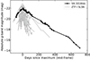 |
Fig. 4. g-band light curve of SN 2018ibb in the context of the homogeneous ZTF-I SLSN sample. SN 2018ibb has a typical peak absolute magnitude. The rise of > 93 rest-frame days is significantly longer than of the average ZTF SLSN. The long-lasting rise implies a long diffusion time, which requires a very high total ejected mass. The high peak luminosity requires a very energetic explosion. Both properties together hint to an explosion mechanism that might be different from that of regular SLSNe. |
A number of SNe have shown a pre-bump with observed peak luminosities between Mg ∼ −18 and −23 mag (Leloudas et al. 2012; Nicholl et al. 2015b; Smith et al. 2016; Angus et al. 2019). Such a bump is not visible in the light curve of SN 2018ibb (Figs. 3 and 4). However, the progenitor of SN 2018ibb exploded before the field came from behind the sun, precluding drawing a firm conclusion on the absence or presence of a pre-bump.
4.2.2. Bolometric light curve
We compute the bolometric luminosity of SN 2018ibb over a wavelength range from ∼1800 to ∼14 300 Å (rest-frame), which is defined by the wavelength coverage of our photometric dataset. However, our dataset does not have the same wavelength coverage throughout the entire duration of the observations. In the following, we describe how the bolometric light curve is constructed and discuss the bolometric corrections that we derived for time intervals with incomplete spectral information.
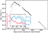 |
Fig. 5. Bolometric light curve of SN 2018ibb from 1800 to 14 300 Å (rest-frame). The dotted lines indicate time segments with partial wavelength coverage. At peak SN 2018ibb reached a luminosity of > 2 × 1044 erg s−1. Integrating over the light curve from tmax–93 to tmax+706 days yields a radiated energy of 3 > ×1051 erg. Both values are conservative lower limits. The inset shows the evolution of the blackbody temperature and radius of the photospheric phase where photometry has been carried out from the u to H bands. The shaded regions indicate the 1σ statistical uncertainties. |
The bolometric light curve is built as follows: (i) correcting all photometric data for the MW extinction, (ii) dividing the entire dataset into segments defined by the observing seasons, (iii) interpolating the light curve in each band of each observing season with a Gaussian process with the python package GEORGE version 0.4.0 (Ambikasaran et al. 2015)13, (iv) constructing the spectral energy distributions for every time step, (v) calculating the bolometric flux by numerical integration of each SED, and (vi) multiplying the bolometric flux by  , where dL is the luminosity distance, to obtain the bolometric luminosity.
Our dataset has the best spectral coverage between tmax and tmax+375 days: 1800–14 300 Å between tmax to tmax+100 days and 3000 to 14 300 Å between tmax+200 to tmax+375 days. The bolometric light curve for these time intervals are shown as solid lines in Fig. 5 and their 1σ confidence intervals as a shaded region. A tabulated version can be found in Table C.1. Based on the blackbody fits to the data from u to H band, we estimate that ≲3% of the observed bolometric flux is emitted at longer wavelengths between tmax and tmax+100 days. Linearly extrapolating the observed SED from 1800 to 14 300 Å towards shorter wavelengths yields a missing UV contribution of ≪1%. Hence, we omit to correct the observed bolometric flux. At later phases, the spectrum does not resemble a blackbody anymore (Fig. 6), and we cannot quantify the missing flux at longer and shorter wavelengths.
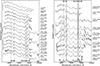 |
Fig. 6. Spectroscopic sequence from 2500 Å to 10 000 Å and from the time of maximum to tmax+1000 days (rebinned to 5 Å and smoothed with a Savitzky–Golay filter). Spectra up to tmax+100 days (left panel) are characterised by a blackbody continuum with superimposed absorption lines from the SN ejecta, expanding with a velocity of ∼8500 km s−1. Between tmax+100 and tmax+225 days (while SN 2018ibb was behind the sun), the spectroscopic behaviour of SN 2018ibb evolved drastically. The late-time spectra (right panel) are characterised in the blue (< 5000 Å) by a pseudo-continuum and emission lines produced by the interaction of the SN ejecta with circumstellar material and in the red (> 5000 Å) by nebular emission lines from the 56Ni-heated SN core. The regions with the fastest evolution are highlighted by the grey-shaded regions. Figure 7 shows the identification of the most prominent features of the photospheric and nebular phases. Regions affected by strong telluric absorption were clipped. Their locations are indicated in Fig. 7. |
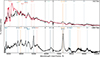 |
Fig. 7. Line identification of the photospheric-phase spectrum (top) and nebular-phase spectrum (bottom). Top: The photospheric phase spectrum was fitted with the parameterised spectral synthesis code SYNOW (red curve). Most of the spectral features can be attributed to O I, Mg II, Si II, Ca II, and Fe II as seen in other SLSNe during their cool photospheric phase (Gal-Yam 2019a). In addition to the absorption lines in the SN ejecta, the photospheric phase spectrum shows conspicuous [Ca II] λλ 7291,7324, a feature that gets dominated by [O II] λλ 7320,7330 at about tmax+30 days. Bottom: The spectrum of the nebular phase consists of a blue pseudo-continuum and a series of allowed and forbidden emission lines from singly and doubly ionised oxygen, calcium, magnesium and iron. Remarkable is the presence of [O II] and [O III] in emission (as early as tmax+30 days), indicating ionising radiation from shock interactions (Sect. 5.1). SN absorption lines are indicated by dashed lines, and the locations mark the absorption trough minima (blueshifted by 8500 km s−1 from their rest wavelengths). SN emission lines are indicated by solid lines; their line centres are at the velocity coordinate v = 0. Regions of strong atmospheric absorption are grey-shaded. |
For the other epochs, we used these time intervals (tmax to tmax+100 days and tmax+200 to tmax+375 days) to estimate bolometric corrections. The pre-max dataset consists of photometry in ZTF g and r, and ATLAS c and o filters, and the Gaia white band. We only use the ZTF data when computing the bolometric luminosity because the ATLAS and Gaia filters are too broad for building SEDs. At the time of the first epoch with coverage from w2 to H, ∼26% of the bolometric flux was emitted in g + r band. We use this flux ratio as an estimate of the missing flux. Since SN ejecta cool with time, such a universal correction will progressively underestimate the bolometric flux towards earlier epochs. Between the first and second observing seasons, we continued the follow-up with Swift/UVOT in ubv when SN 2018ibb was no longer visible from the ground. Similar to the pre-max data, we chose time intervals with data from w2 to H or u to H band to correct for the missing flux. At phases later than tmax+500 days, photometric data are only available from g to z band. We omit to apply any bolometric correction for this time interval because we have no good estimate of the missing bolometric flux.
SN 2018ibb reached a peak luminosity of Lbol, peak ≥ 2 × 1044 erg s−1. Integrating the light curve from tmax–93 to tmax+706 days yields ≥3 × 1051 erg for the total radiated energy Erad. We emphasise that both values are strict lower limits. Our multi-band campaign only started when SN 2018ibb peaked in the g and r bands, which was likely after the bolometric peak.
Between tmax and tmax+100 days, the spectra of SN 2018ibb are characterised by a cooling photosphere (Fig. 6), and the spectral energy distributions from the u to H band are adequately fitted with a Planck function. The red and blue curves in the inset of Fig. 5 show the evolution of the blackbody temperature and radius (see also Table C.1), respectively. The photosphere has a temperature of 12 000 K at the time of maximum light and cools by 3000 K in 100 rest-frame days. During the same time interval, the location of the photosphere hardly changes from its mean value of 5 × 1015 cm. The values of the blackbody radius and temperature are comparable to regular SLSNe (Chen et al. 2023b) and the slow-evolving SLSN 2015bn (Nicholl et al. 2016a), which have observations in the UV. The blackbody temperature of SN 2018ibb evolves slower than for regular SLSNe (Chen et al. 2023b), mirroring its slowly evolving light curve. We remark that including data at shorter wavelengths would have led to lower temperatures (≈0.1 dex at tmax) and larger radii (≈0.12 dex at tmax) due to absorption lines in the UV (Yan et al. 2017; Lunnan et al. 2018a; Angus et al. 2019). Owing to this, we omit these data to infer the blackbody radius and temperature.
4.3. Spectroscopy
4.3.1. Spectroscopic sequence
Figure 6 shows the spectral evolution between ∼2800 Å to ∼10, 000 Å from the time of maximum to tmax+990 days (all rest-frame). The spectra up to tmax+100 days capture the photospheric phase. To identify the elements and ions responsible for the most prominent features, we model the spectrum at tmax+32.7 days with the spectrum synthesis code SYNOW (Branch et al. 2005). The SYNOW fit, shown in the top panel of Fig. 7, was obtained for a photospheric expansion velocity of 8000 km s−1 (Sect. 4.3.2) and for a blackbody temperature of 12 000 K (Sect. 4.2.2; a range in the order of ±500 is applicable for both properties). The major ions that are securely identified and match the spectrum well are those of: O I, Mg II, Si II, Ca II, and Fe II (the Mg II mainly improves the match of the feature around 4400 Å, together with the Fe II line), in agreement with Könyves-Tóth & Vinkó (2021). Various additional iron group elements, such as Ti II, clearly help to lower the model flux on the blue side (3000–4000 Å). However, we do not include those in the final SYNOW fit because the overall fit was not convincingly improved. Intriguingly, the spectrum shows narrow absorption lines from Fe IIλλ 4924,5018,5169 (half-width at zero intensity ≈1500 km s−1), reminiscent of the H-poor SLSNe 1999as and 2007bi. Modelling the photospheric-phase spectra of these two SLSNe revealed that such narrow features are challenging for existing SLSN models (Moriya et al. 2019). These narrow features could point to a velocity cut in the density structure of the SN ejecta. This could be related to the density structure of the progenitor or possibly point to the deceleration of the outermost layer of the ejecta by the collision with dense circumstellar material (Kasen 2004; Moriya et al. 2019). To differentiate between these scenarios, spectral modelling is required. This is beyond the scope of this paper. Absorption from O II between 3700 Å and 4700 Å, as seen in many SLSN spectra around peak (Quimby et al. 2018), is not present.
Owing to the limitations of the SYNOW approach, for instance, the simplifying underlying assumptions such as spherical, homologous expansion, resonant scattering line formation above a sharp blackbody spectrum-emitting photosphere, we perform this modelling only for the identification and verification of the major features. We avoid any fine-tuning of the different ion parameters and assessing the elemental abundances or relative mass fractions.
A complementary analysis with the National Institute of Standards and Technology (NIST) Atomic Spectra Database (Kramida et al. 2018), following the methodology described in Gal-Yam (2019b), which includes the same elements as above for relative intensities ≥0.5 in the range 2000–10 000 Å (and ≥0.2 in the range 3000–6000 Å for the Fe II lines), reveals additional possible identification of features that are not accounted for by the SYNOW fit. For instance, lines of Mg II and/or Si II may contribute to the small dip redwards of the ∼7773 Å (rest-frame) O I triplet. Also, numerous Fe II lines may contribute to the valley around 3000–3200 Å as well as additional Mg II lines accounting for the dips around 4300 Å. Remarkably, in addition to absorption lines from the SN ejecta, the first spectrum at tmax–1.4 days shows conspicuous [Ca II] λλ 7291,7323 in emission. This is one of the strongest forbidden emission lines seen in nebular SN spectra (Filippenko 1997; Gal-Yam 2017). The only SLSNe that show [Ca II] during the photospheric phase are slow-evolving SLSNe (e.g. SN 2007bi, LSQ14an and SN 2015bn; Gal-Yam et al. 2009; Nicholl et al. 2019; Inserra et al. 2017).
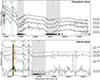 |
Fig. 8. Spectroscopic sequence from 9500 to 21 500 Å. The spectral sequence covers the evolution of the photospheric (top) and nebular (bottom) phases. The NIR spectra at > 1 μm show only a few features in contrast to the optical spectra (Fig. 6). The most prominent features are labelled. All spectra were rebinned to 5 Å and smoothed with a Savitzky–Golay filter, except the spectrum at tmax+361.6 days that was rebinned to 10 Å. The grey scale at the bottom of each panel displays the strength of telluric features (white = transparent, black = opaque). In addition, regions of strong atmospheric absorption are grey-shaded. |
During the first seasonal observing gap, the photosphere recedes and we start to see the core of the explosion. The nebular spectra (right panel in Fig. 6) are dominated by emission lines with widths up to 10 000 km s−1 and a blue pseudo-continuum, similar to that seen in SNe Ia-CSM, Ibn, and Icn and some SNe IIn (e.g. Silverman et al. 2013; Hosseinzadeh et al. 2017; Gal-Yam et al. 2022; Perley et al. 2022). Following previous observations of slow-evolving SLSNe (Nicholl et al. 2016b; Lunnan et al. 2016) and theoretical models by Jerkstrand et al. (2016), we identify the most conspicuous emission lines as allowed and forbidden transitions from neutral and ionised calcium, iron, magnesium, and oxygen (Fig. 7).
Common to both the photospheric and the nebular phase is that the evolution is very slow with the exceptions of the regions at ∼4360, ∼5000 and 7300 Å (highlighted in grey in Fig. 6). At about 30 days after maximum, the region at ∼5000 Å shows a rapidly growing emission feature. A weak emission line at ∼4360 Å also emerges and reveals a similar trend to the ∼5000 Å feature. Owing to this, we identify the two features as [O III] λ 4363 and [O III] λλ 4959,5007, respectively. Most remarkably, the [O III] λλ 4959,5007 emission lines are present throughout the entire post-max evolution, even in the spectrum at tmax+989.2 days after all other SN features faded below the detection threshold of the 4-h VLT spectrum. This has never been observed in any SLSN before. Simultaneous with the rise of [O III], the centre of the 7300 Å feature moves a few Å to longer wavelengths, the line profile changes from roughly top-hat to bell-shaped, the width decreases and the peak flux increases by a factor ∼2 within < 60 days (Fig. 6, left panel). This suggests that this line complex, commonly identified as [Ca II] λλ 7291,7324, gets dominated by [O II] λλ 7320,7330.
[O II] and even more so [O III] are not common features for SNe. [O III] was only observed in the slow-evolving H-poor SLSNe LSQ14an (Inserra et al. 2017) and PS1-14bj (Lunnan et al. 2016) during the photospheric phase and in SN 2015bn in the nebular phase (Nicholl et al. 2016b; Jerkstrand et al. 2017). Occasionally, it is also seen in regular H-poor and H-rich SNe predominantly years after the explosion (e.g. SNe II 1979C and 1980K, Milisavljevic et al. 2009 and Fesen et al. 1999; SN IIb 1993J, Milisavljevic et al. 2012; SNe IIn 1995N, 1996cr, 2010jl, Fransson et al. 2002, 2014; Bauer et al. 2008; Milisavljevic et al. 2012; SN Ib 2012au, Milisavljevic et al. 2018), and even more rarely during the photospheric phase of regular SNe (e.g. Type Ic SN 2021ocs; Kuncarayakti et al. 2022). Possible mechanisms to produce [O II] and [O III] are (i) excitation by CSM interaction (Chevalier & Fransson 1994), (ii) photoionisation by the interaction of the pulsar wind nebula with the SN ejecta (Chevalier & Fransson 1992; Omand & Jerkstrand 2023), and (iii) radioactivity (for high ratios of deposited energy to O-density; Jerkstrand et al. 2017). In Sect. 5.1, we show that [O II] and [O III] are produced by the interaction of the SN ejecta with circumstellar material.
Our series of NIR spectra (shown in Fig. 8) covers the photospheric phase from tmax+33 to tmax+94 days, and the nebular phase from tmax+276 to tmax+378 days. The NIR spectra show a limited number of absorption and emission lines. The photospheric-phase spectra show two features at 1.093 and 1.13 μm. Following Jerkstrand et al. (2015), Hsiao et al. (2019) and Shahbandeh et al. (2022), we tentatively identify the former as an absorption line of Mg IIλ 1.092 μm blueshifted by ∼8500 km s−1, and the latter as the recombination line O Iλ 1.13 μm. These features can also be blended with emission lines from sulphur. The emission lines clearly stand out in the nebular-phase spectra. Our NIR spectra at tmax+378 days show a prominent emission line at 1.025 μm that we tentatively identify as [Co II] λ 1.025. This is the first time that a cobalt line has been detected in a SLSN spectrum. In Sect. 5.2.5, we examine this detection in more detail.
4.3.2. Ejecta velocity
The photospheric-phase spectra of SN 2018ibb show a large number of narrow absorption lines, mirroring a low ejecta velocity and the slow light curve evolution. The ejecta velocities are commonly measured from Fe IIλ 5169. Owing to the high velocities of SLSNe (e.g. Liu et al. 2017; Chen et al. 2023a), this line is usually blended with Fe IIλ 4924 and Fe IIλ 5018, necessitating template matching techniques to extract the velocities (Modjaz et al. 2016; Liu et al. 2017). However, the ejecta velocity of SN 2018ibb is slow, and the Fe IIλ 5169 region is not blended and resolves into three absorption lines that we identify as Fe IIλλ 4924,5018 and 5169 (Fig. 9). By measuring the minima of the three absorption lines, we extract a photospheric velocity of ≈8500 km s−1 that remains constant between tmax and tmax+100 days as demonstrated in Fig. 9 (all measurements are summarised in Table 6).
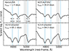 |
Fig. 9. Zoom-in onto the Fe II absorption lines from the SN ejecta at selected epochs of the photospheric phase. The SN photosphere expands with a velocity of merely ≈8500 km s−1. There are no signs of deceleration between tmax and tmax+100 days. Starting at about tmax+30 days, emission from [O III] λλ 4959,5007 (grey shaded region), produced by the interaction of the SN ejecta with circumstellar material, contaminates the blue wing of Fe IIλ 5169. |
Fe II absorption line velocities during the photospheric phase.
The maximum ejecta velocity is best determined from the blue edge of the strong Mg IIλλ 2796,2803 and Ca IIλλ 3934,3968 resonance lines. In Fig. 10, we show the regions around the two features at tmax+32.7 days, centred on the blue doublet components. Because of the complexity of line features, we omit to subtract any continuum. For illustration purposes, we normalise the spectral regions so that the peak intensity and maximum absorption approximately match both lines. The blue components of the doublets exhibit complex profiles at low velocities because of the superposition with the wings of the red doublet components. The highest velocities are less affected by this. The Ca IIλ 3934 line gives the best estimate for the maximum ejecta velocity, ∼ 12 500 km s−1. This is consistent with the extent of the absorption component of Mg IIλ 2796, which, however, is more affected by other SN lines. The absorption minima of Mg IIλ 2796 and Ca IIλ 3934 are at ∼ 8000 km s−1, but are affected by the doublet nature of the lines. Nonetheless, the locations of the absorption minima are consistent with the photospheric velocity determined from the absorption minima of Fe IIλλ 4924,5018,5169.
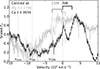 |
Fig. 10. Maximum ejecta velocity. The extent of the Ca IIλ 3934 (black) absorption on the blue side can be traced to ∼ 12 500 km s−1 at tmax+32.7 days. Mg IIλ 2796 (dark grey) has a comparable maximum velocity, albeit this region is affected by additional SN features. The location of the blue and red doublet components of Mg IIλλ 2796,2803 and Ca IIλλ 3934,3968 of the host galaxy ISM are indicated by brackets in a darker shade at the top of the figure. We also mark the position of the doublets of the CSM shell with brackets in a lighter shade. The CSM shell is detected through an additional Mg II absorption-line system blueshifted by 2918 km s−1. The CSM shell is not detected in Ca II. |
To put the measurements in the context of other SLSNe, we first compare the velocity of SN 2018ibb at maximum light to those of SLSNe in the ZTF-I sample (Chen et al. 2023a). The histogram in the top panel of Fig. 11 shows a kernel density estimate of the velocity distribution of the 27 SLSNe from the ZTF-I sample with Fe II velocities measured within ±20 rest-frame days from maximum light. After bootstrapping the sample and propagating the measurement uncertainties with a Monte Carlo simulation, the median velocity of the ZTF-I sample is 14 800 km s−1 and its 1σ confidence region extends from 10 500 to 19 000 km s−1. SN 2018ibb lies in the bottom 8% of this sample, but its velocity is not unparalleled. SN 2019aamu had a lower photospheric velocity at peak, but the measurement is poorly constrained ( ; Chen et al. 2023a). In the bottom panel of Fig. 11, we show the evolution of the Fe II velocities of SN 2018ibb together with those of H-poor SLSNe from Liu et al. (2017; in grey). Within 50 days after maximum, the ejecta usually decelerate from ∼15 000 km s−1 to ≲10 000 km s−1, whereas SN 2018ibb shows no evolution.
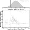 |
Fig. 11. Fe II ejecta velocities of SN 2018ibb and general SLSN samples (grey) at the time of maximum (top panel) and as a function of time (bottom panel). SN 2018ibb has a remarkably low velocity at the time of maximum and an unprecedentedly flat velocity evolution, which is in stark contrast to known SLSNe. |
4.3.3. A CSM shell around the progenitor of SN 2018ibb
The X-shooter spectra between tmax+32.7 days and tmax+94.3 days show two Mg II absorption line systems (Fig. 12). The narrow component is associated with the gas in the SLSN host galaxy (Sect. 4.6). The lines of the broader component have a full width at half maximum (FWHM) of 406 km s−1 and are blueshifted by 2918 km s−1 (not varying between tmax and tmax+90 days; upper panels in Fig. 12). They are significantly broader than expected for the interstellar medium in the dwarf host galaxy or any intervening dwarf galaxy14 but also significantly narrower than the narrowest SN features (∼1900 km s−1; measured from Fe II). The equivalent widths are 2.00 ± 0.09 and 1.27 ± 0.08 Å for Mg IIλ 2796 and Mg IIλ 2803, respectively. The observed line ratio is 1.57 ± 0.12 in tension with the predicted value of 2 for unsaturated lines. Assuming that the Mg II lines are unsaturated, we can convert their equivalent widths to a lower limit on the column density of singly ionised magnesium in the CSM shell. The rest-frame equivalent width EWr is related to the column density N, in units of atoms per cm2, via  where λr is the rest-frame wavelength, in units of Å, and f the oscillator strength (Ellison et al. 2004). Using the oscillator strengths from Theodosiou & Federman (1999) for Mg IIλ 2796 and Mg IIλ 2803, we derive a lower limit of N > 5 × 1013 cm−2.
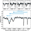 |
Fig. 12. Normalised X-shooter spectra from tmax+32.7 days to tmax+94.3 days (top panels) and their inverse-variance weighted co-added spectrum (bottom panel). The individual and stacked spectra show barely resolved, narrow absorption lines from the host ISM (marked by the solid vertical lines). In addition, a blue-shifted (2918 km s−1) absorption line system is visible (marked by the dashed vertical lines). The FWHMs of the blue-shifted component are 406 km s−1, significantly larger than the ISM lines but significantly smaller than the SN lines. This blue-shifted absorption-line system is connected with a shell of circumstellar material expelled by the progenitor star shortly before the explosion. No significant evolution in the position or shape of the absorption lines can be seen in the individual spectra (upper panels). The error spectrum is shown in grey. |
The only other SLSN that showed such a blueshifted Mg II component was the H-poor SLSN iPTF16eh (Lunnan et al. 2018b). For that SLSN, the Mg II doublet was blueshifted by 3300 km s−1. Lunnan et al. (2018b) also detected Mg II in emission between 100 and 300 days after maximum light. Moreover, the line centre of the emission lines moved from –1600 to +2900 km s−1 during that time interval. These authors attributed the blueshifted Mg II absorption line system with a CSM shell expelled decades before the explosion and the time and frequency variable Mg II emission lines with a light echo from that shell. How such a light echo evolves depends mainly on its distance to the progenitor star. With that in mind, we analyse the Keck and X-shooter spectra between tmax+230 and tmax+378 days to constrain the properties of the CSM shell. Rebinning the spectra reveals Mg II in emission (Figs. 6 and 7). However, due to heavy rebinning, the information about the variability of the line centre was lost. We can, therefore, not ascertain whether the Mg II emission is connected with illuminated magnesium in the CSM shell or produced by the interaction of the SN ejecta with circumstellar material.
Motivated by the discovery of a CSM shell around SN 2018ibb, we next search for corresponding Ca IIλλ 3934,3969 absorption in the X-shooter spectrum from tmax+32.7 (Fig. 10). The search is aggravated by how the two Ca II doublets (CSM shell and SN ejecta) overlap in contrast to the Mg II doublets. Using the wavelength of Ca IIλ 3934 as the velocity reference, the blue doublet absorption of Ca II should be at the same velocity as the Mg II doublet (− 2918 km s−1). The red component of the Ca II doublet will, however, be displaced by 34.8 Å, or 2653 km s−1, to − ∼ 265 km s−1. The position of a possible Ca II CSM component is marked with the light grey bracket in Fig. 10. We do indeed see a sharp drop in the Ca II profile at zero velocity, which could be the result of a red CSM absorption. For the blue component, it is more difficult because we do not know the line profile of the Ca II absorption from the SN ejecta. Therefore, it is difficult to assess the significance of this. However, we conclude that there is no evidence for Ca II absorption from the CSM shell.
4.3.4. Circumstellar interaction – bumps and undulations in the light curve
The multi-band light curves show a series of bumps and wiggles throughout the entire evolution of SN 2018ibb (Figs. 3 and 5). Between tmax and tmax+100 days, the bumps are well visible from u to H band (luminosity increases by a few 0.1 mag). The amplitudes of the bumps in SN 2018ibb are comparable to the bumps seen in light curves of the other SLSNe (e.g. Nicholl et al. 2016a; Inserra et al. 2017; Fiore et al. 2021; Hosseinzadeh et al. 2022; Chen et al. 2023a). Following the nomenclature in Chen et al. (2023a), these bumps fall in the “weak” category. The bumps in SN 2018ibb also introduce wiggles in the evolution of its blackbody radius and temperature (Fig. 5). These modulations are well within the measurement uncertainties of the long-term trends of these parameters, hindering a more in-depth analysis of these features.
The late-time photometric evolution of SN 2018ibb reveals an increase in luminosity of 0.2 dex between tmax+240 and tmax+340 days (Figs. 3 and 5) that is well isolated allowing for a more in-depth analysis. The bolometric light curve before and after this bump exhibits a decline rate of 1.18 mag (100 days)−1. After subtracting the underlying fading light curve, we conclude that the light curve bump lasted for ∼80 days (measured between zero intensity) and reached its highest luminosity at tmax+300 days. In total, 6.7 ± 0.8 × 1048 erg are radiated in excess to the 8.1 × 1049 erg that SN 2018ibb would have emitted without the bump during this time.
Figure 13 presents the spectroscopic evolution of SN 2018ibb during the bump phase. Assuming that all spectral features fade on exponential timescales similar to the multi-band and bolometric light curves, we use the spectra obtained before (blue) and after (yellow) the light curve bump to interpolate the spectrum at tmax+286.7 days (black). Such an approach estimates the spectroscopic behaviour of SN 2018ibb in the absence of the bump. The bottom panel of Fig. 13 shows the observed spectrum at tmax+286.7 days in black and the estimated spectrum without the bump in red. The difference spectrum (blue) reveals substantially enhanced line fluxes in [O II] and [O III] but no change in [O I]. The light-curve bump might also have increased the flux of the continuum level bluewards of 5000 Å. Its shape is reminiscent of the blue pseudo-continuum seen in interaction-powered SNe (Silverman et al. 2013; Hosseinzadeh et al. 2017; Gal-Yam et al. 2022; Perley et al. 2022). Considering the similarity of the difference spectrum to the spectrum before and after the bump raises the question of whether a larger fraction of the emission bluewards of 5000 Å in all nebular spectra is due to CSM interaction. We investigate that further in Sect. 5.2.4.
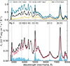 |
Fig. 13. Impact of the light curve bump between tmax+240 and tmax+340 days on the SN spectrum at tmax+286.7 days. Top: The spectra before, during and after the light curve bump. Bottom: The observed spectrum at tmax+286.7 days (≈13 days before the peak of the bump) is shown in black. We estimate the “bump-free” spectrum of SN 2018ibb at tmax+286.7 days (red) based on the spectra obtained before and after the bump. The difference between the observed (black) and interpolated (red) spectra at tmax+286.7 days is shown in blue. It reveals a series of emission lines that can be attributed to [O II] and [O III]. An excess bluewards of 5000 Å is also visible, while no apparent residual can be seen at the location of [O I]. |
4.4. Radio and X-ray emission
The interaction of the SN ejecta with circumstellar material and heating of the SN ejecta by a central engine (e.g. magnetar or a black hole) can produce thermal X-ray emission and non-thermal radio emission (Chevalier & Fransson 1992, 1994). SN 2018ibb was observed in the X-rays and radio between tmax+13 and tmax+246 days (Sects. 3.5 and 3.6). All observations led to non-detections with detection limits between 1 and 6 × 1041 erg s−1 in the X-rays and between 1039 and 1040 erg s−1 in the radio. To put those measurements in the context of the UV-to-NIR bolometric light curve, we show the radio and X-ray measurements together with the bolometric light curve in Fig. 14. From that, we conclude that < 2% and < 10% of the total emission are radiated in the radio and X-rays, respectively.
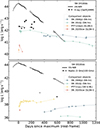 |
Fig. 14. Thermal and non-thermal emission of SN 2018ibb. Less than a few percent of the total radiated energy is emitted in the radio and X-rays. The luminosity limits lie in the ballpark of non-detections of other SLSNe, and they are a factor of 50 larger than the luminosity of the four H-poor SLSNe with either radio or X-ray detection. The limits of SN 2018ibb are larger than the most luminous radio and X-ray SNe. |
The non-detection limits are in the observed range of other SLSNe with X-ray and radio observations (Levan et al. 2013; Coppejans et al. 2018; Margutti et al. 2018; Law et al. 2019; Eftekhari et al. 2021; Murase et al. 2021). Only four SLSNe were detected at X-ray or radio frequencies: PTF10hgi (radio; Eftekhari et al. 2019; Law et al. 2019), PTF12dam (X-ray; Margutti et al. 2018; Eftekhari et al. 2021), SCP06P6 (X-ray; Levan et al. 2013), and SN 2020tcw (radio and X-ray; Coppejans et al. 2021; Matthews et al. 2021). Their measurements15, shown in Fig. 14, are a factor of > 50 smaller than the detection limits of SN 2018ibb.
To put the radio and X-ray properties of SN 2018ibb in the context of interaction-powered SNe, we also show the light curves of the most luminous X-ray and radio SNe in Fig. 14. The Type IIn SNe 2006jd and 2010jl are the most luminous X-ray SNe with absorption-corrected luminosities of ∼1042 erg s−1 (Chandra et al. 2012, 2015). The radio-loudest SNe (e.g. SN Ic-BL PTF11qcj Corsi et al. 2014) reached luminosities of ∼1038 erg s−1, i.e. ≲10 times fainter than the limits for SN 2018ibb. Their observed luminosities before correcting for host absorption can be significantly dimmer for hundreds of days (Chandra et al. 2015).
In conclusion, the non-detection of SN 2018ibb neither rules out CSM interaction nor a central engine as the dominant powering mechanism. Furthermore, the non-detection of SN 2018ibb also agrees with theoretical models of magnetar- and interaction-powered SLSNe that predict no bright radio and X-ray emission for years after the SN explosion (Murase et al. 2016; Margalit et al. 2018; Omand et al. 2018).
4.5. Imaging polarimetry
Our polarimetric observations between tmax+31.9 days and tmax+94.4 days revealed a polarisation signal of 0.27 ± 0.04% in V (weighted average of all epochs) and 0.48 ± 0.07% in the R band (Table 3). Dust grains in the Milky Way and the host galaxy could introduce a polarisation signal. As detailed in Sect. 3.4, the polarisation level of the MW could be up to 0.26%. The level of polarisation from the SN host galaxy is unknown, meaning that all reported measurements are upper limits.
Considering the observed low degree of polarisation and the consistent levels of Stokes parameters measured from SN 2018ibb (Table 3), we conclude that the continuum polarisation intrinsic to SN 2018ibb is ≲0.3% in V band between tmax+31.9 days and tmax+94.4 days. To convert this measurement into an asphericity of the ejecta, we assume an oblate ellipsoidal ejecta with a Thomson scattering atmosphere and a number density distribution of N(r)∝r−n, where r is the ejecta radius and n is the power-law index. Adopting p ≲ 0.3%, we infer an axis ratio B/A (minor axis vs. major axis) of ≳0.9 for an optical depth of τ = 1 and a power-law index of n = 2, and B/A of ≳0.8 for τ = 5 and n = 3 − 5 (Höflich 1991). The degree of polarisation in the R band is slightly higher (p ≈ 0.5%). Therefore, we cannot exclude that the continuum polarisation is p > 0.3%. A polarisation degree p ∼ 0.5% implies an axis ratio B/A of ∼0.88 for τ = 1 and n = 2 (Höflich 1991).
Therefore, we suggest that SN 2018ibb’s photosphere exhibits a high degree of spherical symmetry. Pursiainen et al. (2023) analysed the data of the 16 SLSNe-I with polarimetric observations, including SN 2018ibb. After correcting the phases of all objects for the diverse photometric decline rates, the properties of SN 2018ibb are well within the observed distribution. While some of the events exhibit a non-zero level of polarisation at similar phases to SN 2018ibb (e.g. SN 2015bn and SN 2021fpl; Leloudas et al. 2017; Inserra et al. 2016; Poidevin et al. 2023), most SLSNe show a consistently low polarisation degree at comparable normalised phases (see Fig. 6 in Pursiainen et al. 2023).
The presence of any component in the atmosphere of SN 2018ibb significantly deviating from spherical symmetry is thus unlikely within the photospheric phases covered by VLT polarimetry observations. Although Thomson scattering is wavelength independent, broad emission lines (see spectra in Fig. 6), which are in general not polarised, may dominate the polarisation spectrum in the V band and produce the apparent low polarisation values. Furthermore, iron-group elements in the ejecta (Fig. 7) have a large number of bound-bound transitions in the blue and UV part of the spectrum, which can also depolarise the signal (e.g. Chornock & Filippenko 2008), accounting for the slightly different polarisation levels measured in V and R bands.
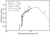 |
Fig. 15. Spectral energy distribution of the host galaxy from 1000 to 60 000 Å (black dots). The solid line displays the best-fitting model of the SED. The red squares represent the model-predicted magnitudes. The fitting parameters are shown in the upper-left corner. The abbreviation “n.o.f.” stands for the number of filters. |
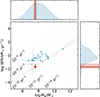 |
Fig. 16. Star-formation rate and stellar mass of the host galaxy of SN 2018ibb in the context of SLSN-I host galaxies from the PTF survey (Schulze et al. 2021). The host galaxy of SN 2018ibb lies in the expected parameter space of SLSN host galaxies but in the lower half of the mass and SFR distributions (kernel density estimates of the observed distributions are shown at the top and to the right of the figure). Its specific star-formation rate (SFR/mass) is comparable to the typical star-forming galaxies (grey band) but lower than for an average SLSN host galaxy. |
4.6. Host galaxy
SN 2018ibb’s host galaxy was detected in several optical broad-band filters (mR ∼ 24.4 mag; Table 1). A false colour image of the field is shown in Fig. 1. The SN explosion site, marked by the crosshair, is ≈1 kpc from the centre of its host galaxy, a common offset for SLSNe (Lunnan et al. 2014; Schulze et al. 2018, 2021). To infer the mass and star-formation rate of the host, we model the observed spectral energy distribution (black data points in Fig. 15) with the software package PROSPECTOR version 1.1 (Johnson et al. 2021)16. We assume a Chabrier IMF (Chabrier 2003) and approximate the star formation history (SFH) by a linearly increasing SFH at early times followed by an exponential decline at late times [functional form t × exp(−t/t1/e), where t is the age of the SFH episode and t1/e is the e-folding timescale]. The model is attenuated with the Calzetti et al. (2000) model. The priors of the model parameters are set identical to those used by Schulze et al. (2021). The observed SED is adequately described by a galaxy model with a stellar mass of  and star-formation rate of
  (grey curve in Fig. 15).
The mass and the star-formation rate of the host of SN 2018ibb agree with the expected values of SLSNe-I host galaxies at z < 0.3 (Leloudas et al. 2015; Perley et al. 2016a; Chen et al. 2017; Schulze et al. 2018, 2021), although both fall in the lower half of the distributions. The specific star-formation rate (SFR normalised by the stellar mass of the host) is comparable to a common star-forming galaxy of that stellar mass (grey band in Fig. 16; Elbaz et al. 2007) but in the lower half of the observed distribution of SLSN host galaxies (Schulze et al. 2021). We caution that specific SFRs are notoriously difficult to measure (e.g. see Fig. 3 in Schulze et al. 2021) as they rely on well-sampled SEDs from the UV to the NIR.
The X-shooter spectra up until Tmax+80 days reveal narrow absorption lines from Mg I and Mg II from the interstellar medium in the host galaxy but no absorption features from Ca II, Fe II, and Mn II, which have prominent features in the wavelength range accessible with X-shooter and are typically seen in low-mass star-forming galaxies, e.g. Prochaska et al. (2007) and Fynbo et al. (2009). The equivalent widths of the detected lines and the upper limits of the strongest expected absorption features are reported in Table 7. The measurements of Mg Iλ 2852 and Mg IIλλ 2796,2804 are comparable to those of the SLSN host galaxies reported in Vreeswijk et al. (2014). Following the methodology of de Ugarte Postigo et al. (2012), we infer an absorption-line strength parameter of ∼ − 3.5 from Ca II, Mg I and Mg II, putting the host of SN 2018ibb at the low-metallicity end of the distribution (albeit the diagnostic is tailored to host galaxies of long-duration gamma-ray bursts, which are also connected with the death of very massive stars but which prefer galaxies with slightly higher metallicities and slightly older stellar populations than SLSNe-I; Hjorth & Bloom 2012; Leloudas et al. 2015; Vergani et al. 2015; Perley et al. 2016b; Schulze et al. 2018).
Properties of the interstellar medium in the host galaxy.
SN 2018ibb’s nebular spectra exhibit emission lines from hydrogen and oxygen from H II regions in the host galaxy. We measure their intensities by integrating over their line profiles. To apply emission-line diagnostics for measuring the oxygen abundance, we also need the flux of [N II] λ 6584, which evaded detection. Using the Hα line profile as a template of the [N II] λ 6584 line profile, we measure the nominal flux and its uncertainty. Table 7 summarises all measurements. Using the O3N2 metallicity indicator with the calibration from Marino et al. (2013) yields a low oxygen abundance of  in accordance with the low value from the absorption-line strength parameter. The oxygen abundance is comparable to the mean of SLSN host galaxies at similar redshifts (Leloudas et al. 2015; Perley et al. 2016a; Chen et al. 2017). The non-detection of [N II] λ 6584 and [O III] λ 4363 adds a systematic uncertainty to the inferred metallicity. However, the average metallicity of a galaxy is correlated with its mass. Andrews & Martini (2013) reported the mass-metallicity relation for star-forming galaxies between z = 0.027 and 0.25, a stellar mass of log M⋆/M⊙ = 7.4–10.5, and metallicities measured with the Te method. Using this mass-metallicity relation yields an oxygen abundance of
  , identical to the value inferred from the galaxy emission lines. Assuming a solar oxygen abundance of 8.67 (Asplund et al. 2009), the host galaxy metallicity is
  solar.
The flux ratio between Hα and Hβ is 2.76 ± 0.62, which is consistent within 1σ with the theoretically expected value of 2.86 for no extinction (assuming a temperature of 104 K and an electron density of 102 cm−3 for Case B recombination; Osterbrock 1989). We conclude that the host attenuation is negligible. The Hα flux translates to a star-formation rate of SFR = 4.4 ± 0.3 × 10⁻³ M⊙ yr−1 using Kennicutt (1998) and the relation from Madau & Dickinson (2014) to convert from the Salpeter to the Chabrier IMF in the Kennicutt (1998) relation. This value is lower than the SFR estimated from the host SED fitting but consistent within 2σ.
5. Discussion
5.1. SN ejecta emission vs. CSM interaction
In Sect. 4.3.3, we have shown that the progenitor of SN 2018ibb is embedded in circumstellar material ejected shortly before the explosion. In this section, we examine the line profiles and evolution of selected oxygen and metal lines to infer the physical conditions of the SN ejecta and the CSM.
The line profiles are most clear in the nebular phase. Figure 17 shows the continuum-subtracted Mg I] λ 4571 line with the [O I] λλ 6300,6364 doublet at tmax+286.7 days. Both lines extend to ∼ 10 000 km s−1. Their maximum velocity hardly changes up to the last well-observed epoch at tmax+637.3 days. Its similarity to the maximum velocity of the Ca IIλ 3934 absorption line (Fig. 10) suggests Mg I] and [O I] are produced in the high-velocity ejecta. The Mg I] line is well fitted with a parabolic line profile with similar maximum velocity, shown by the dark-blue line in Fig. 17. This indicates emission from an optically thick shell with constant velocity (e.g. Fransson 1984).
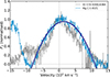 |
Fig. 17. [O I] λλ 6300,6364 and Mg I] λ 4571 lines at tmax+286.7 days. The Mg I] line is well fitted with a parabolic shape (dark blue), expected from an optically thick expanding shell (e.g. swept up CSM and unshocked SN ejecta), while the [O I] lines show a strong blue deficit because the line-forming region is still optically thick. The [O I] doublet is centred on the 6364 Å doublet component. |
A similar parabolic line profile is consistent with the red side of the [O I] λ 6364 doublet component. However, the blue side of the doublet, dominated by the 6300 Å component, lacks most of the emission compared to the Mg I] line. By tmax+637.3 days (Fig. 18), the blue doublet component has grown and is now the stronger of the two lines. The evolution of the [O I] line profile may be explained if both doublet components are optically thick to at least tmax+286.7 days. In that case, the blue component will be scattered by the red component, which extends over most of the blue component (the velocity difference between the two components is 3016 km s−1). These photons will either be thermalised or emerge on the red side of the 6364 Å doublet component. Emission from the front side of the ejecta with velocities ≲ −(v − 3016 km s−1 ) are only partially scattered, and some of this emission may leak out, explaining the “bump” at ∼ −7500 km s−1. At tmax+565.0 days, the blue doublet component has grown, and the blue wing is equally bright, or somewhat brighter, compared to the 6364 Å component. This trend continues at tmax+637.3 days. The expected 3:1 ratio is still not reached, indicating that the ejecta is not optically thin, yet.
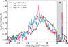 |
Fig. 18. Late-time evolution of the [O I] λλ 6300,6364 doublet. Note the strong evolution on the blue side, while the red side of the lines is evolving slower. This indicates a transition from optically thick to optically thin [O I] lines, implying that the scattering in the absorption part of the P Cygni profile is decreasing. Regions of strong atmospheric absorption are grey-shaded. |
Using the Sobolev (1957) theory for the line formation, we can estimate the optical depth τ for a given O I density n(O I) in the ejecta (e.g. Li & McCray 1992). Assuming LTE among the 3P ground state levels, the optical depth of each line of the [O I] doublet is given by
where A(1D2, 3PJ) with J = 2, 1 are the transition probabilities for the 6300 Å and 6364 Å lines, respectively,  is the wavelength of blue and red doublet component, respectively, gtot = 9 is the total statistical weight to the ground multiplet, and t is the time since the explosion, in units of day. Putting in the atomic constants, we get an optical depth for the 6364 Å line of
and a depth that is a factor of 2.9 larger for the 6300 Å line. The typical O I density needed to get an optically thick line is, therefore, ≳109 cm−3. This can be compared to the mean oxygen density of the core. Assuming O I is the dominant species of oxygen in the core, the number density is
 (1)
(1)
where M(O) is the mass of oxygen in the core, f is the filling factor, and vej the ejecta velocity. To get an optically thick 6364 Å line at tmax+286.7 days, in other words a density ≳1010 cm−3, requires a very small oxygen filling factor, ≲10−3 (i.e. a highly clumped medium), or an unphysically large oxygen mass of ≳103 M⊙.
In a CSM and PPISN interaction scenario, the continued high optical depth at late times could point to a highly compressed cool dense shell (CDS). A CDS will form from the compression behind the shock, which results from the interaction between the ejecta and the CSM (for a discussion see, e.g. Chevalier & Fransson 2017). If the density of the CSM is large, the forward shock will be radiative and dominate the emission, which will then have the composition of the CSM. In the opposite case, the reverse shock dominates with a composition typical of the outer ejecta. The latter case is more relevant for lower mass loss rates. In both cases, the density enhancement behind the cooling shock will be very large. Assuming an approximate pressure balance behind the shock, the density enhancement will be of the order of  , where μ is the mean molecular weight (∼1.7 for a fully ionised oxygen gas), mu the atomic mass unit, vrel the relative velocity between the CSM shell and the ejecta, Tshock the temperature immediately behind the shock, and Tps the post-shock temperature in the CDS (∼104 K). With vrel ≈ 5000 km s−1 17, the compression is of the order of 105. Both vrel and Tps are uncertain and magnetic pressure could limit the compression. The CDS is also most likely unstable (Chevalier & Blondin 1995), leading to clumping of the shell and limiting of the compression. However, the estimate shows that a very large density could result in the CDS, making the line optically thick, equivalent to a low filling factor. In the PISN scenario, strong clumping in the ejecta is needed. This is, however, not indicated from simulations of PISN models without CSM by Chen et al. (2020).
We now turn to the origin of the higher ionisation [O II] and [O III] lines. Figure 19 shows the line profiles of the [O I], [O II] and [O III] lines after subtracting the continuum. Owing to the doublet nature of the lines, we centre the line profiles on the blue component in the left panel and on the red component in the right panel. These line widths can be compared to the velocity of the CSM shell, the photospheric velocity, and the maximum velocity of the ejecta (vertical lines in Fig. 19). It is clear that the [O II] and [O III] line widths are closer to the velocity of the CSM shell than to the photospheric velocity of the SN ejecta; in contrast to the [O I] line, which extends to the maximum velocity of the SN ejecta.
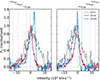 |
Fig. 19. [O I] λλ 6300,6364, [O II] λλ 7320,7330, and [O III] λλ 4959,5007 line profiles at tmax+565.0 days. The velocity scale is centred on the blue doublet component in the left panel and on the red component in the right panel. [O II] and [O III] only reach out to approximately the velocity of the CSM shell (vCSM), much less than the photospheric velocity (vFeII) and the maximum velocity of the ejecta (vmax). In contrast to that, the [O I] profile extends to ⊈ 12 500 km s−1. This points to [O II] and [O III] being produced close to the CSM shell whereas [O I] is produced in the SN ejecta. |
The differences in the origin of the forbidden oxygen lines are corroborated by the O I–O III line profiles (Figs. 19 and 20). The asymmetric [O III] λ 4363 and [O III] λλ 4959,5007 lines have little emission in the red wings indicative of emission from a thin shell, where most of the red emission is absorbed by the photosphere. Examples of this can be seen in Fig. 4b in Fransson (1984). That scenario is also consistent with the evolution of the [O II] λλ 7320,7330 doublet. The 7300 Å line, which may be a blend of the [O II] λλ 7320,7330 lines and [Ca II] λλ 7291,7324, is shown in Fig. 21, centred on the [O II] λ 7320 line. Focusing on the [O II] lines (left panel), the blue wing has a nearly constant line profile between tmax+231.2 and tmax+565.0 days. The red wing of the [O II] λ 7330 doublet component gets considerably narrower during the same time interval. At tmax+637.3 days (right panel), the entire 7300 Å line profile changes quite dramatically, becoming flat-topped and broader. This is a result of the [Ca II] λλ 7291,7324 lines becoming strong, while the [O II] lines get weaker.
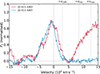 |
Fig. 20. Comparison of the [O III] λλ 4959,5007 lines with the [O III]λ 4363 line. These lines are produced by the interaction of the SN ejecta with circumstellar material. Due to the occulation of the CSM by an optically thick SN ejecta, less of the “backside” of the CSM is seen. The velocities of the CSM shell (vCSM), the photospheric velocity (vFeII) and the maximum velocity of the ejecta (vmax) are indicated. |
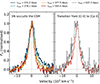 |
Fig. 21. Evolution of the [O II] λλ 7320,7330 + [Ca II] λλ 7291,7324 line complex. Left: Up to tmax+565.0 days, the line complex is dominated by [O II]. The red wing narrows due to an increasing occultation of the CSM shell by the optically thick expanding SN photosphere. Right: Between tmax+565.0 days and tmax+637.2 days, the line complex shifts to the blue, consistent with the [Ca II] line becoming more dominant. All profiles are centred on [O II] λ 7320. |
The increasing asymmetry of the [O II] doublet may be qualitatively understood by the CSM being occulted by the SN ejecta. Assuming that the optically thick SN ejecta with the velocity vej slams into the CSM shell with a low velocity (ideally v ≈ 0) located at a distance Rs from the progenitor star, the maximum velocity of the red wing vred is (a pure geometric effect)
where Δt is the time between the shell ejection and the explosion and t the time since explosion. (We have assumed that t ≪ Δt.) Because the ejecta with the CDS, which may define the photosphere, expands with a much higher velocity (∼ 8500 km s−1 vs. ∼ 3000 km s−1) a progressively increasing portion of the dense CSM will be occulted by the photosphere and less of the “backside” of the CSM will be seen. This would lead to the red side getting narrower with time. At the same time, an increasing portion of the dense CSM will be shocked, leading to a decreasing luminosity from the dense CSM, including the [OII–III] emission.
The fact that the forbidden [O II] and [O III] lines are seen at about tmax+30 days adds additional constraints on the physical conditions where they originate. The critical densities, above which collisional de-excitation becomes important, are less than ∼2 × 106 cm−3 for [O II] and [O III] (Osterbrock & Ferland 2006). This is much lower than the densities expected in the ejecta (Eq. (1)). Therefore, the [O II] and [O III] lines would be severely suppressed if they were coming from the ejecta. Not only do [O II] and [O III] originate from the CSM, but also the recombination lines O Iλ 7773 and O Iλ 9263. The blue wings of their line profiles are similar to [O II] λ 7320, extending to ∼ 5000 km s−1 (Fig. 22).
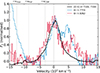 |
Fig. 22. Comparison of the [O II] λλ 7320,7330 lines with the O Iλ 7773 and O Iλ 9263 recombination lines. The similar line profiles, extending to ≲ 5000 km s−1 indicates an origin in a highly processed CSM shell. |
In summary, we propose a two-component scenario where the broad component, seen in particular in the [O I] λλ 6300,6364 and Mg I] λ 4571 lines as well as the broad absorption in Mg IIλ 2800 and Ca IIλ 3934 come from either the CDS or possibly the unshocked ejecta. The low-velocity component seen in the [O III] lines, as well as the [O II] and O I recombination lines come from the CSM shell at ∼ 3000 km s−1. The fact that we see [O III] λλ 4959,5007 emission even at tmax+989.2 days means that the dense CSM must extend out to at least a few ≈1017 cm. The velocity width of the Mg II absorption of the CSM shell of 406 km s−1 (Sect. 4.3.3; Fig. 12) may correspond to the velocity gradient over the CSM shell. That we do not see any change in the width with time suggests that this gradient must be small enough so that the velocity close to the shock is nearly constant. The origin of this gradient is not clear, though. One explanation could be that this is the result of a time-limited eruption, where a Hubble-like outflow is expected after a few dynamical time scales. This has been observed, for instance, in the Eta Carinae Homunculus nebula produced during the great eruption in 1843 (e.g. Smith 2006). The absence of H and He lines throughout the entire evolution reveals (Fig. 6) that the CSM shell must be processed gas from the stripped progenitor. Any hydrogen and helium must have been lost before this eruption and reside at much larger radii.
Among the > 200 H-poor SLSNe known, SN 2018ibb is only the seventh object with spectroscopic evidence of CSM interaction. In previous cases, CSM interaction did not manifest itself via [O III] in emission (a possible candidate for CSM interaction with O-rich material is PS1-14bj; Lunnan et al. 2016). iPTF16eh revealed CSM interaction through a light echo produced in a shell of H-poor and He-poor material (Lunnan et al. 2016). Late-time spectra of iPTF10aagc, 13ehe, 15esb and 16bad (Yan et al. 2015, 2017) and SN 2018bsz (Pursiainen et al. 2022) showed broad Balmer emission lines, suggesting that their progenitors lost their hydrogen envelopes much closer to the time of the terminal explosion than SN 2018ibb and iPTF16eh.
5.2. Constraints on the powering mechanism and progenitor
In the following, we contrast SLSN and PISN models with our photometric and spectroscopic datasets and discuss the most likely powering mechanism and progenitor of SN 2018ibb.
5.2.1. Modelling the bolometric light curve
We first analyse the bolometric light curve. Katz et al. (2013) proposed an exact method for testing whether a light curve is powered by the decay of radioactive material and, therefore, allows us to place an upper limit on any 56Ni produced during the explosion of SN 2018ibb’s progenitor. This method is independent of details in the radiative transport, including the highly uncertain opacity, the velocity distribution and the ejecta geometry. The method is described in detail in Wygoda et al. (2019) and Sharon & Kushnir (2020). In brief, the Katz integral is given by
and ET is the integrated time-weighted luminosity that would be emitted if no 56Ni were produced. Assuming that there is no additional source of energy, ET can be assumed to be negligible. The total energy deposition rate from radioactive decay of 56Ni, Qdep, is given by Jeffery (1999)
where t0 is the γ-ray escape time. The deposition rates from γ-ray photons and positrons are
where the mean lifetimes of 56Ni and 56Co are t1/2,Ni = 8.76 days and t1/2,Coi = 111.4 days, respectively (Junde 1999).
Since the explosion time is not well known, we vary the explosion time between 0 and 50 rest-frame days before the first detection and use the relation L/LT = Q/QT to determine the γ-ray escape time. We measure a range of 600–700 rest-frame days for t0. After the γ-ray escape time is determined, we infer the nickel mass by comparing the luminosity in the fitted range to the deposited radioactive energy. The best fit for each point in the texp grid is shown in Fig. 23. Indeed, the declining light curve is fully consistent with being powered by 24–35 M⊙ of 56Ni. The upper bound could be even larger if the SN explosion happened more than 50 rest-frame days before the detection by Gaia.
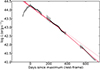 |
Fig. 23. The bolometric light curve of SN 2018ibb from 1800 to 14 300 Å (rest-frame) and light-curve fits to the fading light curve using the Katz et al. (2013) method. The entire fading light curve from up to 706 days after peak is fully consistent by being powered 24–35 M⊙ of 56Ni (dark red), suggesting that SN 2018ibb could be a pair-instability supernova. At about 300 days after peak (i.e. ≳400 days after the explosion), the γ-ray trapping decreases with time. The loss of trapping is indicated by the difference between the light-red (100% trapping) and dark-red (< 100% trapping) curves. |
The rise time of 90–140 days, the range of γ-ray escape times and the range of nickel masses are consistent with expectations from PISN models (Kasen et al. 2011; Kozyreva & Blinnikov 2015; Kozyreva et al. 2017) and SN Ia18 (another class of thermonuclear explosions; e.g. Wygoda et al. 2019; Sharon & Kushnir 2020), after scaling their average nickel mass to the nickel mass of SN 2018ibb. Both the excellent match with nickel powering and coverage of the fading light curve for 706 days is unprecedented for any of the > 200 SLSNe known, suggesting that SN 2018ibb could indeed be a PISN.
5.2.2. Modelling the broadband light curve
Next, we fit the multi-band light curve with the Modular Open-Source Fitter for Transients MOSF IT software tool (Guillochon et al. 2018). In addition to the MOSF IT NICKEL model that is based on the parameterisation by Nadyozhin (1994), we also select the central-engine models SLSN (describing powering by a spin down of a magnetar; Nicholl et al. 2017) and FALLBACK (describing powering by a black hole accreting fallback material; Moriya et al. 2018c), and the Chatzopoulos et al. (2012) model to characterise the powering by CSM interaction. We also utilise the more complex models MAGNI combining powering by a magnetar and radioactive 56Ni (Blanchard et al. 2019) and CSMNI which combines powering by CSM interaction and 56Ni. In all models, the photosphere is assumed to have a blackbody spectral energy distribution at all times. While this approximation is adequate during the photospheric phase, it is inadequate at later times when the spectrum is dominated by emission lines and an interaction-powered pseudo-continuum. The spectral energy distribution of the model SLSN is modified in the UV to account for absorption by the SN ejecta. As our dataset covers a very long time span, the trapping of γ-ray photons will eventually decrease, which accelerates the fading. All chosen models include a component to account for the loss of trapping (Nicholl et al. 2017).
The priors of the model parameters are chosen to cover a broad range of the physically allowed parameter spaces. Their ranges and shapes are similar to Nicholl et al. (2017), Kangas et al. (2022) and Chen et al. (2023b), and they are summarised in Table 8. For the pure nickel model, we set the opacities κ and κγ to 0.07 and 0.027 g cm−2, respectively (Swartz et al. 1995; Wang et al. 2015, and references therein). For the models that include two sources of energy, in which one of the energy sources is 56Ni, we perform fits with unconstrained opacities as well as fits with the opacities set to κ = 0.07 g cm−2 and κγ = 0.03 g cm−2. The model parameters are inferred in a Bayesian way using the nested sampler DYNESTY. The fits of each model are shown in Fig. 24. As the fit covers a wide time interval, each panel in Fig. 24 also contains a window zooming in onto the region of maximum light. The marginalised posteriors of the model parameters are summarised in Table 8.
Light-curve fits with MOSF IT: models, parameters, priors and marginalised posteriors.
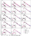 |
Fig. 24. Modelling of the light curves from the rest-frame UV to the NIR with MOSFiT. All models provide an adequate description of the data up to tmax+400 days, though with differences in the fit quality. At later times, the models diverge. The pure nickel model is the only model that captures the evolution after tmax+500 days and has physically meaningful parameters. The central engine models (magnetar and fallback) predict a flattening of the light curve due to a power-law-shaped heating rate in contrast to powering by 56Ni that has an exponential energy deposition rate. The magnetar+nickel model also captures the full evolution. However, the inferred model parameters would be either physically implausible or require an exotic star, which we deem not viable. We note that the Keck photometry at tmax+539 days and tmax+562 days is not corrected for host contamination owing to the lack of Keck reference images to perform image subtraction. The expected host contribution is ≈10%. |
Visually, all models capture the rise, peak and decline up to tmax+400 days. There are noticeable differences between the fits and the data because of (i) not all models can be correct, (ii) the inherent assumptions of each model, and (iii) the assumption of a blackbody photosphere at all times. Owing to this, none of the models can capture the bumps and undulations (see inset in Fig. 24). The significant deviation in the z band at > tmax+200 days is due to the assumption of a blackbody photosphere. The late-time spectra reveal a blue pseudo-continuum with super-imposed emission lines. The luminescent [O II] λλ 7320,7330 emission lines are redshifted to the z band and cause the apparent discrepancy between the data and the models (Fig. 6).
Besides these general caveats, differences in the fit qualities between the models are visible. At epochs later than tmax+500 days, the pure central engine models fail to describe the data. The discrepancies grow with time and reach ∼2 mag per band at tmax+706 days. In contrast to that, all nickel and CSM models are able to describe the entire light curve from tmax–93 days to tmax+706 days. The fundamental difference in the late-time behaviour of the central-engine and nickel models lies in how the models deposit energy into the ejecta (and hence the SN luminosity). In the pure central engine models, the energy deposition evolves as a power law in time. This leads to a decrease in the decline rate of the SN brightness in the time vs. magnitude space. In contrast to that, radioactive material has an exponentially declining energy deposition rate. This results in a linear decline in the time vs. magnitude space, which fits our observations well. The loss of γ-ray trapping accelerates the fading independent of the powering mechanism, but it only modifies the light curve without altering its general shape. In other words, the loss of gamma-ray trapping cannot convert a power-law decline into an exponential decline (e.g. Chen et al. 2015; Wang et al. 2015; Nicholl et al. 2018).
The nickel models (56Ni and 56Ni+CSM|magnetar) provide an adequate fit to the entire light curve. All models require ≈35 M⊙ (spread in the median values: 20–63 M⊙; statistical error of the individual measurements: 7–67%; Table 8) of freshly synthesised nickel, consistent with our conclusions on the bolometric light curve (Sect. 5.2.1). The pure 56Ni has a worse fit statistic because of the loss of γ-ray trapping. This leads to underpredicting the expected brightness. This is not a critical issue. The modelling assumes that the SED is still a blackbody, which is not the case anymore (Sect. 5.2.4). Furthermore, fitting the bolometric light curve with 56Ni gave an excellent fit (Sect. 5.2.1. Such large nickel masses can only be produced in a PISN explosion. PISN models predict no remnant after the entire star is obliterated (Fowler & Hoyle 1964; Barkat et al. 1967; Rakavy et al. 1967), eliminating the magnetar + 56Ni model. If we were to ignore stellar evolution theory, the rotational energy of the magnetar, which defines how much energy could be converted into radiation, would contribute < 1% to the total radiated energy (∼1 × 1050 erg), whereas > 99% of the radiated energy would come from the radioactive decay of 56Ni and its daughter products (Table 8). Moreover, the inferred spin period of ∼15 ms is much larger than the median spin period of ∼2.6 ms from the ZTF-I SLSN sample (Chen et al. 2023b, see also Nicholl et al. 2017 and Blanchard et al. 2020). Even the slowest spinning SLSN magnetars never exceeded 6–7 ms (Nicholl et al. 2017; Blanchard et al. 2020; Chen et al. 2023a)19.
The CSM + 56Ni model might be viable. However, the inferred nickel fraction and CSM parameters are very sensitive to the a priori unknown effective opacities κ and κγ. The two parameters are different for each radiation component and come with their own uncertainties. Furthermore, the contribution of CSM interaction and 56Ni to the observed light curve changes with time resulting in a time-variable κ and κγ. Capturing these complexities is not possible with that particular CSM + 56Ni model. Furthermore, the Chatzopoulos et al. (2012) CSM model used in MOSF IT is debated (see the discussion in Sorokina et al. 2016; Moriya et al. 2018a), limiting the interpretability of the results. More sophisticated CSM + 56Ni models are needed to disentangle the two sources of energy (e.g. Chevalier & Fransson 2017; Tolstov et al. 2017a; Suzuki & Maeda 2021; Takei et al. 2022).
The pure magnetar model can be rejected on physical and statistical grounds. The aforementioned increased over-prediction of observed flux at late time makes this model unviable. Furthermore, the magnetar model requires extreme conditions (MNS ∼ 2.1 M⊙, P0 = 1 ms and Mej ∼ 81 M⊙) to squeeze out as much energy as possible from the neutron star. The lower limit on the progenitor mass (Mprogenitor > Mej + MNS) exceeds 83 M⊙. Explosion models predict that such a massive star leaves behind a black hole but not a neutron star (Heger & Woosley 2002). From an empirical point of view, the H-poor SLSNe, which are thought to be powered by a magnetar, have ejecta masses of only ∼5 M⊙. The most massive ejecta reach a few 10 M⊙ but never exceed 50 M⊙ (Nicholl et al. 2017; Blanchard et al. 2020; Tinyanont et al. 2023; Chen et al. 2023a; West et al. 2023), in stark contrast to the ∼81 M⊙ required to power SN 2018ibb. Previously, Eftekhari et al. (2021) reported that SN 2018ibb is powered by a magnetar (using the same magnetar model) but using a very sparse data set. We caution against this practice. Even with our comprehensive data set, only the data after tmax+600 days broke the degeneracy between the central-engine models and the nickel-powered models. Furthermore, the best-fit magnetar properties presented here and in Eftekhari et al. (2021) are significantly different, demonstrating that datasets with a large wavelength coverage and a wide time span are required to determine the powering mechanism of SLSNe. Our results echo the conclusions from Moriya et al. (2017), who performed a parameter study of magnetar and nickel models, that the two models could produce indistinguishable light curves if the data set covers only a limited time interval. Very late-time observations, such as those presented here, are critical to break the degeneracy in the light curve modelling (Moriya et al. 2017).
The fallback model has implausible parameters. The total energy input from the fallback accretion required to power the light curve is given by  (Moriya et al. 2018c). For the best-fit values (Table 8), we infer a total energy input of 0.9–4.4 M⊙ c2. Assuming a realistic conversion efficiency from the fallback accretion disk to the large-scale outflow of 10−3 (i.e. the SN luminosity; Dexter & Kasen 2013), the mass of the accretion disk would have to be 900–4400 M⊙, which is unphysical. In the case of a jet forming during the accretion process, the conversion efficiency could be ∼10% (McKinney 2005; Kumar et al. 2008; Gilkis et al. 2016) and the mass of the accretion disk would only have to be 9–44 M⊙. Irrespective of the accretion efficiency, the fallback model always over-predicts the brightness by ∼2 mag at late times. To mitigate this issue, the accretion rate would also have to be fine-tuned to match observations. Owing to these issues, we do not deem the fallback model to be viable for SN 2018ibb.
To strengthen our conclusions on the model selection, we also fit the observations using the software package REDBACK (Sarin et al. 2023), which implements these different models. We fit the multi-band data in magnitude space with a Gaussian likelihood function and the exact same priors, and utilise the NESTLE 20 sampler implemented in BILBY (Ashton et al. 2019; Romero-Shaw et al. 2020). The fit parameters of the pure magnetar and nickel models as well as the magnetar + nickel model are consistent with the results from MOSF IT (Table E.1). The pure nickel model is the only viable model. Furthermore, the necessity for a large ejecta is solely determined by the long rise. It does not depend on the availability of the data in the blue bands. We verified that by fitting the data in the r band and in redder filters with MOSF IT and REDBACK (Tables 8 and E.1).
In summary, the multi-band light curve is consistent with being powered by radioactive 56Ni. The undulations, visible in several bands, are not captured by this nickel model. This could point to an additional source of energy, for example, interaction with circumstellar material. The required 56Ni mass of ∼35 M⊙ can only be produced during a PISN explosion. Central engine models can be excluded with high confidence. The necessity for a large ejecta and nickel mass is solely determined by the long rise, the high peak luminosity and the slow decline. It does not depend on the availability of the data in particular filters.
Due to this extraordinary result, we want to briefly comment on whether the derived ejecta mass (Mej ∼ 83 M⊙), nickel fraction (∼50%), velocity (∼ 4000 km s−1) and kinetic energy (14 × 1051 erg) are sensible for PISN models (values taken from Table 8). The PISN models by Kozyreva et al. (2017), Gilmer et al. (2017) and Heger & Woosley (2002) predict for a progenitor with a nickel yield of ∼35 M⊙ an ejecta mass of ∼130 M⊙, a nickel fraction of ∼30%, an ejecta velocity of 9000–11 000 km s−1 and a kinetic energy of 80–90 × 1051 erg. The model-predicted ejecta velocities, kinetic energy and nickel fractions appear to be in tension with our results, but that is not critical for the following reasons. (i) The nickel model used in the light-curve fitting is an analytical one-dimensional model, but not a PISN model. (ii) The velocity of the nickel model is a scaling velocity, which is not the ejecta velocity. In Sect. 4.3.2, we showed that the ejecta velocity is 8500 km s−1. The fastest portions of the ejecta move at ∼ 12 500 km s−1. These velocities yield a more realistic kinetic energy of 60–130 × 1051 erg, consistent with PISN model predictions. (iii) Different light-curve fitting codes give slightly different results. (iv) PISN models have large uncertainties in predicting the energy release and the amount of 56Ni. They depend on the nuclear network and assumptions of a given stellar evolution code, such as convection, details of the solution of the stellar structure equations and the dynamical phase of the pair-instability explosion, etc. For example, 56Ni masses calculated by Takahashi (2018) and Umeda & Nomoto (2002) differ significantly from Heger & Woosley (2002). In Umeda & Nomoto (2002), a 270 M⊙ star would produce 10 M⊙ of 56Ni and a similar star in Takahashi (2018) would produce between a few M⊙ masses and > 30 M⊙ of 56Ni. In contrast to that, a 250 M⊙ star in Heger & Woosley (2002) yields ∼55 M⊙ of 56Ni. As shown by Farmer et al. (2019, 2020) and Kawashimo et al. (2023), the choice of the 12C(α, γ)16O reaction rate leads to the scatter in the final 56Ni mass between 10M⊙ and 70 M⊙ for the He-core stellar model of 130 M⊙, and a factor of 2 in the amount of the released explosion energy.
5.2.3. Matching the light curve with PISN templates
Motivated by the light-curve fits, we compare the bolometric light curve to the PISN templates from Kasen et al. (2011), Gilmer et al. (2017) and Kozyreva et al. (2017). The grid of models from Kasen et al. (2011) are the metal-free helium models from Heger & Woosley (2002). The Gilmer et al. (2017) and Kozyreva et al. (2017) models assume a metallicity of 7% solar. Very massive stars in low-metallicity environments (Z ∼ 0.07 Z⊙) lose their hydrogen envelopes during the early evolution, assuming up-to-date wind mass-loss rates. The details about the used mass-loss rates are described in Ekström et al. (2012) and Yusof et al. (2013). Therefore, these stars are hydrogen-free by the time of the pair-instability episode, and the helium-core models from Heger & Woosley (2002) are a good representation of these explosions. This is in agreement with the models from Gilmer et al. (2017). Their suite of models, which were computed self-consistently, are initially hydrogen-rich models; however, owing to mass loss, the highest-mass models become hydrogen-free by the time of the explosion.
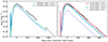 |
Fig. 25. Comparison of SN 2018ibb with the PISN models P250Ni25 and P250Ni34 from Kozyreva et al. (2017; left panel) and the He100, He125, and He130 from Heger & Woosley (2002; right panel). Templates with nickel masses of 34–44 M⊙ are required to describe the entire bolometric light curve from tmax–93 to tmax+706 days. Models with M(Ni)=25 M⊙ systematically underestimate the observed bolometric light curve, but they could still be viable if CSM interaction contributes significantly throughout the evolution. |
Among the suitable models, we chose the P250Ni25 and P250Ni34 templates from Gilmer et al. (2017), and the He100, He120, He125 and He130 templates from Kasen et al. (2011; where the number stands for the helium core mass in M⊙). The models have nickel yields between 5.8 and 40 M⊙. The vital properties of these models are presented in Table 9. The P250Ni25 model starts with an initial mass of 250 M⊙. At the time of the explosion, a helium core of 127 M⊙ has formed, which is similar to the helium models He125 and He130. We note that the P250Ni25 model not only loses its hydrogen envelope but also most of its helium layer (total mass of 2.6 M⊙ before the loss of the He layer) and ends up as a bare carbon-oxygen core with a tiny helium fraction by the time of the pair-instability explosion. In contrast to that, the He125 and He130 models evolve without mass losses and retain 2.4 M⊙ and 2.8 M⊙ of helium, respectively.
Summary of PISN model parameters.
To build the bolometric light curves of the PISN models, we use the hydrodynamics radiative transfer code STELLA (Blinnikov et al. 2006). The slight difference of the P250Ni34 light curve between our calculation and that in Gilmer et al. (2017) and Kozyreva et al. (2017) is caused by the different versions of STELLA used in the two studies. A relevant discussion can be found in Kozyreva et al. (2020). The re-calculated light curves of the helium models are consistent with those calculated with the spectral synthesis code SEDONA (Kasen et al. 2011). In Fig. 25, we compare the bolometric light curve of SN 2018ibb to those computed for a series of PISN models. The PISN templates with nickel yields between 34 and 44 M⊙ (He125, He130, P250Ni34) provide excellent matches to the rise, the peak, and the fading parts of the bolometric light curve of SN 2018ibb. While the He125 and P250Ni34 models describe the rise and peak well, they systematically underestimate the late-time flux. Such a deviation at the late epochs may not necessarily refute these two models since the observed bolometric flux of SN 2018ibb may include a time-varying contribution from CSM interaction. As we show in Sect. 5.2.4, this contribution is not negligible and could boost the luminosity by a few 0.1 dex.
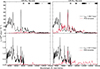 |
Fig. 26. Late-time spectra of SN 2018ibb at 287 and 637 days after its maximum. Overlaid are the computed PISN spectra from Jerkstrand et al. (2016) scaled to these epochs. The shaded region indicates the uncertainty of the explosion time. The He130 model provides an adequate description of the emission redwards of 6000 Å at tmax+286.7 days, but a worse match for the second epoch. The observed spectra show a considerable excess at shorter wavelengths that is not expected from the model spectra. We argue that the blue excess is due to the interaction of the SN ejecta with circumstellar material, which is not included in existing PISN models. The He100 model matches the observation of neither epoch. The vertical bars at the top of each panel indicate the location of telluric features. |
The templates with M(Ni)∼25 M⊙ (He120 and P250Ni25) also provide reasonable matches to the data, even though they exhibit a faster rise and produce peak luminosities that are ≈0.3 dex fainter. In the case that CSM interaction contributes at all times, the apparent tension might be alleviated. The PISN model He100, which produces the smallest amount of Ni in our set, generates a light curve that is incompatible with observations. The peak bolometric luminosity of such a model is 0.8 dex lower compared to the observed value, implying that a different energy source must account for > 84% of the observed peak luminosity.
5.2.4. Late-time spectra of SN 2018ibb compared to PISN models
Jerkstrand et al. (2016) computed spectra of the He100 [M(Ni)=5.8 M⊙] and He130 [M(Ni)=44 M⊙] PISN models at 400 and 700 days after the explosion21. To compare these spectra with the observations, we need to constrain the poorly measured explosion date of SN 2018ibb. The bolometric light curve of the He100 and He130 models peaked at ≈130 rest-frame days. Assuming that SN 2018ibb’s bolometric light curve peaked up to 20 days before the peak in the g|r band, we can scale the computed spectra to the epochs of the observed spectra via exp(Δt/t1/2, Co), where Δt is the phase difference between the observed and computed spectra and t1/2, Co is the mean lifetime of 56Co.
Figure 26 shows the observed spectra of SN 2018ibb at tmax+286.7 (top row) and tmax+637.3 days (bottom row) in black. The upper left and the bottom left panels compare the earlier and the later spectra with the phase-adjusted He100 model (red) at tmax+400 days and tmax+700 days, respectively. The right column presents the same comparison to the He130 model spectra. The phase-adjusted spectra have a shaded band to indicate the impact of the uncertain peak time of the bolometric light curve on the model flux. We selected the observed spectra at these specific epochs to minimise the phase correction and cover a wide wavelength range.
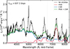 |
Fig. 27. Nebular spectrum of SN 2018ibb (black) at tmax+637.3 days and its decomposition into a CSM interaction (blue) and PISN component (red). This decomposition reveals that the shape of the spectrum in the blue is similar to the pseudo-continuum seen in interaction-powered SNe (Type Ia-CSM, Ibn, Icn and IIn). The emission lines in the blue arise either from CSM interaction or from material in the CSM shell excited by the SN light. The dotted vertical lines indicate the location of strong galaxy emission lines. |
The He100 model fails to match the spectra of SN 2018ibb at both tmax+286.7 and tmax+637.3 days. The predicted emission lines are significantly weaker compared to the data, and the relative strength of the features does not match the shape of the observed spectra. In addition, the model spectra also exhibit lines that are significantly narrower compared to the observed spectra since the He100 model yields a lower ejecta velocity (Table 9). The He130 model provides a better match. At tmax+286.7 days, the model spectrum describes the observed spectrum redwards of 6000 Å well, in terms of the absolute and relative strength of the features as well as the line widths. The computed spectrum also matches the observed NIR spectrum, albeit the strongest predicted feature at 1.2 μm (Fe I and Si I) is redshifted to a region that is strongly affected by atmospheric absorption (indicated by the black-shaded region in the upper half of the figure). The match at tmax+637.3 days appears to be less plausible compared to that at tmax+286.7 days. While the model reproduces the [O II]+[Ca II] at 7300 Å, the observed spectrum shows an elevated continuum level and stronger [O I] λλ 6300,6364 in emission. The observed spectrum also shows prominent O Iλ 7773 in emission that is not generated by the model. However, in Sect. 5.1 we showed that O Iλ 7773 is produced by the CSM interaction.
Bluewards of 6000 Å, the discrepancy between the observed and computed spectra is considerable in both epochs. A similar excess in the blue part of the spectrum was observed in other slow-evolving SLSNe (e.g. Jerkstrand et al. 2017), and it was used as a critical piece of evidence against the PISN interpretation (e.g. Dessart et al. 2013; Nicholl et al. 2013). Mazzali et al. (2019) performed detailed modelling of a nebular phase spectrum of the candidate PISN 2007bi and confirmed these conclusion from Dessart et al. (2013), Nicholl et al. (2013) and Jerkstrand et al. (2017). In addition, these authors put forward the idea that if the core of the explosion was mixed, Ca, Mg and O would become efficient coolants and would produce conspicuous emission lines at 4570 Å (Mg), 6300,6363 Å (O), and 7291,7324 Å (Ca). However, PISN calculations do not support the notion of mixing in the inner ejecta (Mazzali et al. 2019; Chen et al. 2020).
This blue excess is not a critical piece of evidence against the PISN interpretation for SN 2018ibb. In Sects. 4.3.3, 4.3.4 and 5.1, we showed that SN 2018ibb is not solely powered by 56Ni. SN 2018ibb’s progenitor had an eruptive mass-loss episode shortly before the explosion. The interaction of the SN ejecta with CSM contributes to the observed light curve via discrete emission lines, and it could even produce a blue pseudo-continuum similar to that seen in interaction-powered SNe (Silverman et al. 2013; Hosseinzadeh et al. 2017; Perley et al. 2022)22. This raises the questions of whether the blue excess in SN 2018ibb is similar to that seen in interaction-powered SNe and how large the contribution of CSM interaction is to the bolometric light curve.
In Fig. 27, we further inspect the spectrum of SN 2018ibb at tmax+637 days against the phase-adjusted spectrum of the He130 model. We attempt to decompose the spectrum of SN 2018ibb into two elements, namely a PISN and an ejecta-CSM interaction component. The CSM component is represented by a spectrum of the Type Icn SN 2021csp obtained at ∼52.7 days after the explosion from Perley et al. (2022) 23. Its flux scale is scaled so that the sum of the PISN and CSM components (green) matches the shape of SN 2018ibb’s pseudo-continuum. This approach is similar to that in Ben-Ami et al. (2014), where these authors used a spectrum of a Type IIn SN to deduce that the ejecta of the Type Ic SN 2010mb interacted with a large amount of H-free circumstellar material. Indeed, this toy model captures the general shape of SN 2018ibb, suggesting that a considerable fraction of the flux bluewards of 6000 Å is produced by the CSM interaction. Most of the emission lines in the blue and O Iλ 7773 feature were not observed in the spectrum of SN 2021csp. However, we have shown that some of the observed lines in SN 2018ibb, for example, O Iλ 7773,9262, [O II] λλ 7320,7330 and [O III] λλ 4959,5007, are generated by the CSM interaction. Others, such as [O I] λλ 6300,6364 and Mg I] λ 4571, are likely formed in the unshocked SN ejecta or the contact discontinuity (cool-dense shell) between the SN ejecta and the CSM (Sect. 5.1).
Assuming SN 2018ibb’s progenitor is similar to the He130 star model, we can roughly estimate the fractions of the observed bolometric flux that have been produced by the nickel decay and the CSM interaction. The bolometric luminosity calculated at tmax+286.7 days covers the wavelength range from 3020 to 14 250 Å (rest-frame). The phase-adjusted model spectrum from Jerkstrand et al. (2016) accounts for 70% of the bolometric flux. In other words, the nickel-powered light curve would be 0.1 dex fainter than the observed bolometric light curve. At tmax+637.3 days, the observed bolometric luminosity covers the range from 3930 Å to 8500 Å (rest-frame). The phase-adjusted PISN spectrum accounts for only 21% of the observed bolometric flux. This means that the Ni-powered light curve would be 0.7 dex fainter. To illustrate that, we show in Fig. 28 the observed bolometric light curve (solid blue lines) and the fraction of the observed bolometric light curve that can be attributed to the He130 model (dashed red lines).
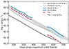 |
Fig. 28. Observed late-time bolometric light curve (solid blue lines) and the fraction of light that could be attributed to 56Ni after accounting for CSM interaction (dashed, red). The dotted green curves show the 56Ni light curve after adding the missing IR flux (up to 5 μm). The IR correction pushes the light curves back to the regime of PISN models that produce 25–44 M⊙ of 56Ni. Even in the case of a substantial contribution from CSM interaction, a total amount of 25–44 M⊙ of 56Ni appears to be essential to power SN 2018ibb. |
However, there is a critical detail that we need to take into account before drawing a conclusion. The bolometric light curves of the P250Ni25|34 and He100–He130 models extend to 50 000 Å. Therefore, our observed bolometric light curve could miss a substantial fraction of the true bolometric flux. The Jerkstrand et al. (2016) model spectra cover the wavelength range from the far UV to 25 000 Å, and Fig. 13 in Jerkstrand et al. (2016) shows the fraction of light emitted between 25 000 Å and 50 000 Å, allowing us to estimate the missing IR fractions. At tmax+286.7 days, the missing IR fraction is 0.14 dex. This fraction increases to ∼0.39 dex at tmax+637.3 days, due to the shorter wavelength coverage of the observed bolometric light curve and an increased mid-IR contribution from the PISN model. The dotted green line in Fig. 28 shows the estimated Ni-powered light curve of SN 2018ibb after correcting for the missing IR flux. The IR correction fortuitously compensates for most of the observed bolometric flux lost to CSM interaction, corroborating that even with significant CSM interaction a total mass of 25–44 M⊙ of 56Ni is still needed to power the light curve and spectra.
A progressively increasing contribution from CSM interaction to the bolometric flux is not a contrived scenario. If the shock is radiative, as is expected for a high metallicity and dense CSM, then the luminosity from the shock is  , where Δvrel is the relative velocity of the ejecta and the CSM. If the density gradient, n, of the ejecta is steep, the shock velocity is only slowly decreasing, vs ∝ t−1/(n − s) for a CSM with r−s density profile, and the shock luminosity will only be a slowly decreasing function of time (Chevalier & Fransson 2017). Because the radioactive input decreases exponentially, it is expected that the shock contribution will increase relative to the radioactively powered input.
5.2.5. [Co II] λ 1.025 μm
The NIR spectra of SN 2018ibb after tmax+300 days reveal an emission line at 1.025 μm that we interpret as [Co II] (a triplet of individual lines at 1.019, 1.025 and 1.028 μm, which result from the 9-1, 10-2, and 11-3 transitions as sorted from higher to lower energies, respectively; Fig. 29). The line luminosities are (2.9 ± 0.8)×1040 erg s−1 and (5.4 ± 1.4)×1040 erg s−1 at tmax+352.6 and tmax+377.5 days, respectively. Assuming optically thin LTE, we can convert the line luminosity to a (temperature-dependent) Co II mass. The line luminosity of the [Co II] λ 1.025 μm multiplet can be written as the sum of the individual transitions

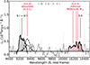 |
Fig. 29. Zoom-in of the region from 9000 Å to 10 500 Å at tmax+377.5 days. Cobalt has its strongest feature at 1.025 μm. Its tentative detection translates to 56Ni mass of ≳30 M⊙, consistent with the light curve modelling. The second strongest cobalt feature is at 9340 Å. Its location is indicated by a fiducial Gaussian centred 9340 Å. Its integrated luminosity is expected to be between 50 and 100% of [Co II] λ 1.025 μm. The absence of [Co II]λ 9340 is not an argument against the discovery of [Co II] λ 1.025 μm (see Sect. 5.2.5 for details). Lines from other elements that could blend with the [Co II] lines are marked. Regions of strong atmospheric absorption are indicated by vertical bars at the top of the figure. |
where Nu is the total number of ions in the upper state u, Au − l the transition rate for spontaneous emission from the upper state u to the lower state l, and Eu − l the energy level of the transition. We use Quinet (1998) for the values of the Einstein coefficients and the energy levels. The partition function can be taken as 20, with an error less than a factor of 2 for reasonable temperatures. Then, using Eq. (42) in Jerkstrand (2017), the cobalt mass is given by
![Mathematical equation: $$ \begin{aligned} M\left(\mathrm{{\text{Co}}{\small {{\text{ II}}}}}\right) \gtrsim 0.5\,M_\odot \,\times \,\left[\frac{L\left(\mathrm{{\text{Co}}{\small {{\text{ II}}}}}\right)}{5\times 10^{40}\,\mathrm{erg\,s^{-1}}}\right] \times \frac{\exp {\left(15410/T\right)}}{\exp {\left(15\,410/5000\right)}}, \end{aligned} $$](/articles/aa/full_html/2024/03/aa46855-23/aa46855-23-eq91.gif)
where T is the temperature of the ejecta, in units of K. The temperature factor (the ratio of exponentials) varies from 0.2 at T = 10 000 K to 100 at T = 2000 K.
To calculate the initial nickel mass, we need to account for the amount that has decayed over time. The initial nickel mass is a factor of exp(t/t1/2, Co) ≳ exp(450/111) ≃ 60 larger, where t is the time since explosion and t1/2, Co is the mean lifetime of 56Co. Averaging over the line luminosities of the two epochs, the inferred 56Ni mass is ≳30 M⊙ if T ≈ 5000 K. This estimate is consistent with the inferred 56Ni mass from the light-curve modelling (Sects. 5.2.1–5.2.3). However, lower values of the nickel mass would be expected if the temperature is higher (6 M⊙ at T = 10 000 K). For temperatures below ∼3500 K, the nickel mass becomes unphysically large, > 100 M⊙. We note that [Co II] λ 1.025 μm can be blended with S IIλ 1.032 μm24, indicated by the hatched region in Fig. 29.
This Ni-mass estimate assumes that the transitions are optically thin. The Sobolev optical depth of the 9-1 transition line in LTE is (Jerkstrand et al. 2017, ignoring stimulated emission):
![Mathematical equation: $$ \begin{aligned} \tau _{9,1} &= A_{9,1}\,\lambda _{9,1}^3\,\frac{1}{8 \pi } \frac{g_9}{g_1}\,n_1 t\\&\approx 0.08 \times \left(\frac{M\left(\mathrm{{\text{Co}}{\small {{\text{ II}}}}}\right)[450d]}{1\,M_\odot }\right) \frac{x_1}{f}, \end{aligned} $$](/articles/aa/full_html/2024/03/aa46855-23/aa46855-23-eq92.gif)
where λ9, 1 is the wavelength of the emitted photon, gn is the multiplicity of the nth state, n1 is the number density of atoms in the ground state, x1 is the fraction of Co II ions in the ground state, and f is the filling factor for the 56Ni zone. In LTE at 5000 K x1 is ≈0.5, whereas at lower temperatures and/or in NLTE x1 is typically higher (towards unity). A typical CCSN has a characteristic filling factor of f ∼ 0.1 for any given zone, which means that 0.5 M⊙ of 56Co are optically thin at ∼450 days. For SLSNe, filling factors for the oxygen zones have been derived to be f ≈ 10−3 − 10−2 (Jerkstrand et al. 2017). If these filling factors also hold for the 56Ni zone of SN 2018ibb, then the Co II lines would be optically thick at ∼450 days, and determining a mass from them would be impossible at that time (Jerkstrand 2017). One may note that numerical simulations of PISNe show little clumping or mixing of the inner material (Chen et al. 2020), and the low filling factors derived for other SLSNe may be due to mixing from the central engine (e.g. Suzuki & Maeda 2021) or compression by circumstellar interaction (van Marle et al. 2010).
In the stripped-envelope-supernova models from Jerkstrand et al. (2015), [Co II] λ 1.025 μm is the strongest predicted line from cobalt. The second strongest Co feature is a blend of two lines at 9338 and 9344 Å. This [Co II] feature could be blended with the red wing of the O Iλ 9263 recombination line. In optically thin LTE, the expected line ratio between [Co II] λ 9340 and [Co II] λ 1.025 μm is between 0.5 − 1 for a wide range of plausible temperatures. To examine whether [Co II] λ 9340 could be present in the spectrum at tmax+387 days, we show in Fig. 29 a Gaussian centred at 9340 Å that has either the same integrated luminosity as [Co II] λ 1.025 μm or a luminosity that is 50% smaller. Clearly, [Co II] λ 9340 is not present in our data at those luminosities.
In the He130 model of Jerkstrand et al. (2016) at 400 days after the explosion, neither of the [Co II] lines are present in any significant strength as they are absorbed by line blocking extending into the NIR. Under conditions with less line blocking (as in the Jerkstrand et al. 2015 CCSN models), the [Co II] λ 1.025 μm line can still be visible, also as iron has few strong emission lines around this particular wavelength. The same cannot be said about the 9340 Å region where iron is stronger. In a PISN ejecta, the densities are about 100-times higher for a given epoch, and the NIR region is still largely opaque at 400 days after the explosion. To explain the observed [Co II] λ 1.025 μm line but the absence of the [Co II] λ 9340 feature, we need to call upon absorption of the 9340 Å line but not the 1.025-μm line. In other words, the He130 model reproduces the spectral shape near 9340 Å but not at 1.025 μm if SN 2018ibb is a PISN.
While the association of [Co II] λ 1.025 μm could be the smoking gun signature that SN 2018ibb is a PISN, we caution that the interpretation hinges on the detection of a single line. An IR spectrum with NIRSpec (Jakobsen et al. 2022) aboard the James Webb Space Telescope could resolve such ambiguity. It is the only instrument that can provide an uncensored view from 1 to 5 μm. Such a spectrum could reveal, for instance, Co, Fe and Ni lines at > 2.7 μm as seen in the Type Ia SN 2021aefx (Kwok et al. 2023).
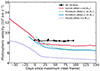 |
Fig. 30. Photospheric velocity evolution of SN 2018ibb (probed with Fe II) and the predicted evolution from different PISN models. The synthetic velocities of the P250Ni25|34 and He130 models are very similar to the observed velocities and velocity evolution. These are also the models that match the observed bolometric light curve well, in particular the He130 model. |
5.3. Velocity evolution
In Sect. 4.3.2, we showed that the photospheric velocity is ≈ 8500 km s−1 and remained constant between tmax and tmax+100 days. Here, we contrast our observations with predictions of PISN models.
From the observational point of view, the photospheric velocity is defined via the minimum of the Fe IIλλ 4924,5018,5169 P Cygni profiles, which serve as a good proxy of the photospheric velocity (Dessart & Hillier 2005). In contrast to that, there is no specific location of the photosphere from the radiative transfer point of view, because its location is wavelength dependent. An average photosphere could be estimated, for instance, via the Rosseland mean optical depth (Rybicki & Lightman 1986) and electron scattering.
The photospheric velocity of the light curves simulated with STELLA is defined as the velocity of the mass shell where the integrated optical depth in the B band is equal to 2/3. The integrated optical depth accounts for the total opacity, which includes contributions from continuum opacity (photoionisation, free-free absorption, and electron scattering processes assuming local thermodynamical equilibrium in the plasma) and line interactions. The location of the photosphere defined with this method coincides to a large extent with the location of the electron-scattering photosphere (Kozyreva et al. 2022) and permits a direct comparison with our observations.
The velocity evolution of the P250Ni25, P250Ni34, He100, and He130 PISN models together with the observed Fe II velocities are shown in Fig. 30. The match between the observed and predicted velocity tracks of the P250Ni25|34 and He130 models is very good in both the predicted velocities and the velocity evolution, in particular the He130 model. Small deviations exist in the absolute values of the velocities (He130: |vobs − vpredicted| ≲ 1000 km s−1 and P250Ni25|34: |vobs − vpredicted| ∼ +2000 km s−1) but not the velocity evolution. These discrepancies are in part due to differences in the definitions of the synthetic velocity and the physical model used in STELLA. Furthermore, none of the parameters of the PISN models were tuned to fit the observations. The velocity track of the He100 model is inconsistent with the observations (|vobs − vpredicted| ≳ +3000 km s−1). As shown in Sect. 5.2.3, the predicted bolometric light curve of this model also does not match the observations.
5.4. Comparison to other slow-evolving SLSNe
Among the ≳200 H-poor SLSNe known, only eight objects belong to such a phenomenological subclass of slow-evolving SLSNe: SN 1999as (Hatano et al. 2001), SN 2007bi (Gal-Yam et al. 2009), PS1-11ap (McCrum et al. 2014), PTF12dam (Nicholl et al. 2013), LSQ14an (Inserra et al. 2016), PS1-14bj (Lunnan et al. 2016), SN 2015bn (Nicholl et al. 2016a) and SN 2018ibb.25 In the following sections, we compare the photometric and spectroscopic properties of SN 2018ibb to those of the historical slow-evolving SLSNe to comprehensively examine its exceptional properties. We omit SN 1999as from this analysis because its light curve and spectra were never published.
We utilise the multi-band and bolometric light curves and host-subtracted spectra of LSQ14an presented in Inserra et al. (2017) and Jerkstrand et al. (2017), PS1-11ap from McCrum et al. (2014), PS1-14bj from Lunnan et al. (2016), PTF12dam from Nicholl et al. (2013), Chen et al. (2015) and Quimby et al. (2018), SN 2007bi from Gal-Yam et al. (2009), Young et al. (2010) and Jerkstrand et al. (2017), and SN 2015bn from Nicholl et al. (2016a,b, 2018) and Jerkstrand et al. (2017). Furthermore, we use the Fe II velocity measurements from Liu et al. (2017) and Lunnan et al. (2016). All light curves and spectra were corrected for MW extinction. The spectrum of SN 2015bn in Nicholl et al. (2018) is not corrected for any host contribution. In Appendix F, we describe our approach to subtract the host contamination for SN 2015bn.
Light-curve properties of slow-evolving SLSNe.
5.4.1. Light curves
Following the methodology of Chen et al. (2023b), we measure for each slow-evolving SLSN the k-corrected peak absolute magnitude in the g band, the k-corrected rest-frame g − r colour, and the 1/e rise and decline time-scales of the g-band light curves26. All measurements are summarised in Table 10. We also report in that table the measurements of SN 2018ibb and, for a broader comparison, the median values of the homogeneous ZTF SLSN sample (Chen et al. 2023b).
Slow-evolving SLSNe, including SN 2018ibb, have peak absolute magnitudes between ∼ − 20.8 and −22 mag in the g band and k-corrected g − r colours between −0.2 and 0 at peak (Table 10). Both their absolute peak magnitudes and the peak g − r-colours are comparable to the median values of the ZTF SLSN sample (median values being Mg, peak − 21.5 mag and g − r = −0.12 mag; Table 10). The rising parts of the light curves of the historical slow-evolving SLSNe are not well sampled, limiting the comparison with SN 2018ibb and the ZTF SLSN-I sample. Only PS1-14bj has a rise time that is at least as long as that of SN 2018ibb and even 30 days longer than that of SN 2018ibb. The decline time scales of the historical slow-evolving SLSNe are well measured. They vary between 38 and 130 days, placing those events above the average of the ZTF-I sample (Table 10). Yet, only one historical slow-evolving SLSN had a decline time-scale as extreme as SN 2018ibb. With a decline time scale of 130 days, PS1-14bj evolves even slower than SN 2018ibb but its peak luminosity in the rest-frame g-band was 1.2 mag fainter than that of SN 2018ibb. This makes SN 2018ibb an unprecedented case even among the most extreme SLSNe known. LSQ14an also has a decline time scale of 100 days, but the observed light curve only covers the declining light curve, adding an unknown systematic error to its time scale measurement.
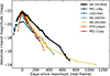 |
Fig. 31. SN 2018ibb in the context of the phenomenological sub-class of slow-evolving SLSNe. Even among this rare sub-class of SLSNe, SN 2018ibb with its exceptionally broad light curve and high peak luminosity is an extreme object with unprecedented properties. |
Figure 31 shows the r-band absolute magnitude light curves of all slow-evolving SLSNe. The supernovae 2015bn and 2018ibb are the only SLSNe with observations extending beyond 500 rest-frame days after maximum light. The light curve of SN 2015bn faded much faster than that of SN 2018ibb. At about 400 days after peak, the decline slowed down and became very gradual. In contrast, SN 2018ibb’s light curve faded linearly with a decline slope of ∼1.1 mag (100 days)−1 that steepened to ∼1.5 mag (100 days)−1 at 500 days after maximum. These differences translate into differences in the powering mechanisms. Magnetars lose their rotational energy efficiently through dipole radiation, which scales as Ėrot ∝ t−2. The energy deposition (and henceforth the SN luminosity) evolves as a power law. Therefore, the light curve is expected to flatten at later times (in the time vs. magnitude space). Radioactive material has an exponentially declining energy deposition rate, which results in a linear decline in the time vs. magnitude space. The loss of γ-ray trapping accelerates the fading independently of the powering mechanism, but it only modifies the light curve without altering its general shape, i.e. the loss of gamma-ray trapping cannot convert a power-law decline into an exponential decline (e.g. Chen et al. 2015; Wang et al. 2015; Nicholl et al. 2018). Therefore, the power-law-shaped decline of SN 2015bn could point to magnetar powering, as concluded in Nicholl et al. (2018). In return, SN 2018ibb’s continued linear decline excludes powering by a magnetar.
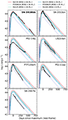 |
Fig. 32. The bolometric light curves of SN 2018ibb and historical slow-evolving SLSNe in the context of PISN models with nickel masses between 5 and 44 M⊙. SN 2018ibb is the only SLSN whose entire light curve from tmax–93 to tmax+706 days is consistent with PISN templates. The other SLSNe have either too fast declining light curves, light curve shapes inconsistent with PISN models, or their light curves are poorly sampled, hindering a comparison with PISN templates. The grey-shaded region indicates the 1σ uncertainty. |
Nicholl et al. (2017) fitted the multi-band data of the slow-evolving SLSNe with the SLSN magnetar model in MOSF IT. This model provides an adequate description of the observations, even to the data of SN 2015bn at 1000 rest-frame days after maximum (Nicholl et al. 2018). The best-fit parameters cover the range from 5.3 to 14 M⊙ for the ejecta mass Mej (median being 6.3 M⊙), 0.1 to 0.8 × 10¹⁴ G for the orthogonal component of the magnetic field strength B (median being 0.3 × 10¹⁴ G), and 2.3 to 3.9 ms for the initial spin period P0 (median being 2.8 ms). These values are typical for SLSN light curves fitted with that particular magnetar model (Nicholl et al. 2017; Chen et al. 2023a). SN 2018ibb has starkly different values (Sect. 5.2.2; Table 8). The best fit requires a magnetar with an initial spin period of 1 ms and an ejecta mass of 86 M⊙, to squeeze out as much energy as possible from the magnetar model. As alluded to in Sect. 5.2.2, such massive stars do not have neutron star remnants. Furthermore, the magnetar model overpredicts the late-time flux significantly due to its power-law-shaped energy deposition.
In Fig. 32, we compare the bolometric light curves of the slow-evolving SLSNe to the suite of PISN models used for SN 2018ibb in Sect. 5.2.3. The bolometric light curves of all historical slow-evolving SLSNe are either inconsistent with the PISN models or the comparison is inconclusive: PTF12dam evolves too fast, the light curves of PS1-11ap and SN 2015bn have a different shape to PISN templates, PS1-14bj shows a flattening at late times, and the bolometric light curves of SN 2007bi and LSQ14an have no pre-max data. The lack of an estimate of the rising bolometric light curve for the latter two objects precludes concluding whether the two SLSNe could be PISNe or not. Dedicated studies on PS1-11ap, PS1-14bj, PTF12dam and SN 2015bn revealed that the magnetar model provides an adequate description of the light curves (Nicholl et al. 2013, 2018; McCrum et al. 2014; Lunnan et al. 2016; Vurm & Metzger 2021).
In conclusion, SN 2018ibb is the only SLSN among the hundreds of SLSNe known whose entire light curve is consistent with PISN models. This result is even more revelatory considering that the bolometric light curve covers an exceptionally wide time interval from tmax–93 to tmax+706 days.
5.4.2. Spectra
In this section, we compare the spectroscopic properties of SN 2018ibb to those of other slow-evolving SLSNe. First, we compare the photospheric velocities measured with the Fe IIλ 5169 region. The top panel of Fig. 33 displays the photospheric velocities, measured from the Fe IIλ 5169 region, of SN 2018ibb and other slow-evolving SLSNe27 (in colour) and of the ZTF-I sample (kernel density estimate). The slow-evolving SLSNe have velocities between 8000 and 12 000 km s−1 at peak, lower than the median value of the ZTF-I sample (14 800 km s−1). PTF12dam and SN 2015bn have the fastest expanding ejecta (∼12 000 km s−1 at peak), but their ejecta rapidly decelerate to ∼6000 km s−1 in ∼60 rest-frame days. Their velocities and velocity evolution is similar to those of other SLSNe (Liu et al. 2017). In stark contrast to that, SN 2018ibb has a velocity of merely 8500 km s−1, comparable to those of PS1-14bj and SN 2007bi. Furthermore, the velocity of SN 2018ibb remains constant for 100 rest-frame days, which has not seen for any other SLSN before. Though the velocities of PS1-14bj and SN 2007bi are very similar to SN 2018ibb, the spectroscopic sequences of these two events are limited, precluding comparing their velocity evolution to that of SN 2018ibb.
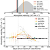 |
Fig. 33. Fe II ejecta velocities of slow-evolving SLSNe (in colour) and general SLSNe samples (grey) at the time of maximum (top panel) and as a function of time (bottom panel). SN 2018ibb has a markedly low velocity at the time of maximum and a flat velocity evolution, which is in stark contrast to the bulk of the SLSN population. Its velocity at peak is similar to the slow-evolving SLSNe PS1-14bj and SN 2007bi. However, both comparison objects lack spectra at earlier and later times. |
Next, we explore the spectroscopic properties of slow-evolving SLSNe during their photospheric and nebular phases. Panel A in Fig. 34 shows the photospheric spectra at the time of maximum light. PTF12dam and SN 2015bn sustained a hot photosphere with a temperature of ≳12 000 K (Nicholl et al. 2016a; Vreeswijk et al. 2014). One of the strong features in their spectra is a comb of O II absorption lines, a characteristic feature of SLSNe, which are only seen in photospheres with T > 15 000 K (Quimby et al. 2018) and probably also require non-thermal excitation (Mazzali et al. 2019). The spectra of PS1-11ap, PS1-14bj and SN 2018ibb are cooler (blackbody temperatures of 10 000–12 000 K). Their spectra do not show O II absorption lines but instead absorption lines from Ca, Fe, Mg, O and Si (see Fig. 7 for the locations). Common to PTF12dam, SN 2015bn and SN 2018ibb is the presence of [Ca II] λλ 7291,7323 in emission. It is one of the strongest features seen in nebular phase spectra of SNe (Filippenko 1997; Gal-Yam 2017) but is only seen during the photospheric phase in slow-evolving SLSNe (Gal-Yam et al. 2009; Inserra et al. 2017; Nicholl et al. 2019). It is also seen in SN 2007bi and LSQ14an, but these SLSNe lack spectra at peak.
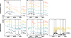 |
Fig. 34. Comparison of the spectra of SN 2018ibb to those of other slow-evolving SLSNe between tmax+30 days and tmax+1000 days (darker colour: 5 Å binning; light shade: unbinned spectra). Photospheric phase (Panels A–B): Around tmax (Panel A), the spectra of PTF12dam and SN 2015bn are characterised by a hot continuum with superimposed O II absorption lines as seen in many SLSNe at a similar epoch. SN 2007bi, LSQ14an and SN 2018ibb have cooler photospheres, and their spectra exhibit absorption lines from Ca, Fe, Mg, O and Si (see Fig. 7 for their locations) but not O II. At around tmax+60 days (Panel B), all spectra appear similar, though differences exist. LSQ14an, PS1-14bj, and SN 2018ibb are the only SLSNe showing [O III] in emission. Furthermore, SN 2007bi, LSQ14an and SN 2018ibb exhibit strong [Ca II]+[O II] in emission. This feature is also present in PTF12dam and SN 2015bn but is less pronounced. Nebular phase (Panels C–E): Differences start to emerge during the early nebular phase and become stronger with time. SN 2018ibb, LSQ14an and PS1-14bj continue to show conspicuous [O III] in emission, in contrast to PTF12dam, SN 2007bi and SN 2015bn that have very strong [O I] and O I in emission. SNe 2015bn and 2018ibb are the only SLSNe with spectra at ∼tmax+1000 days (Panel E). SN 2018ibb continues to show intermediate-width [O III], whereas the spectrum of SN 2015bn exhibits [O I]. The elevated noise in the SN 2018ibb spectrum at tmax+989.2 days at λ > 6000 Å is due to residuals of the skyline subtraction. The dashed vertical lines indicate the expected locations of emission lines commonly seen from H II regions. |
Around the time of maximum light (Panel B), all objects have similar spectra. Due to the differences in the ejecta velocities, features appear sharper in LSQ14an, PS1-14bj and SN 2018ibb that in PTF12dam and SN 2015bn. Some clear differences are well visible though. LSQ14an, PS1-14bj and SN 2018ibb reveal [O III] in emission. As we concluded in Sect. 5.1, the 7300 Å feature in SN 2018ibb is not dominated by [Ca II], but [O II] λλ 7320,7330. In the other objects, the centre of the 7300 Å feature is consistent with [Ca II]. Moreover, the 7300 Å feature is well developed in SN 2007bi, LSQ14an and SN 2018ibb but still very weak in PTF12dam and SN 2015bn. The line profiles also differ. In SN 2018ibb the line profile is flat-topped but triangular and skewed to the blue for the other objects.
During the early nebular phase (t/tdecline ∼ 2; Panel C), all objects show a blue pseudo-continuum with superimposed forbidden and allowed emission lines from calcium, magnesium and oxygen (for the line identifications see Fig. 7). SN 2018ibb and PS1-14bj are spectroscopically indistinguishable, though their overlap in wavelength is limited and PS1-14bj is significantly fainter than SN 2018ibb (Fig. 31). The other objects reveal an increasing level of dissimilarities (LSQ14an → SN 2015bn → SN 2007bi). LSQ14an has a similar blue pseudo-continuum but its emission lines are not well developed. This is best seen in Ca IIλλ 3933,3968, [O III] λ 4363 and [Ca II] λλ 7291,7324 + [O II] λλ 7320,7330. The SNe 2007bi and 2015bn have redder pseudo-continua and significantly weaker [Ca II]+[O II]. Moreover, SN 2007bi has only a few features bluewards of 5000 Å.
These differences develop further with time. During the late nebular phase (t/tdecline ∼ 5; Panel D), the pseudo-continuum of all objects fades. SN 2018ibb and LSQ14an are characterised by a weaker [O I] λλ 6300,6364 than SNe 2007bi and 2015bn. The ratio between [Ca II]+[O II] and [O I] is 2–3:1. Intriguingly, the emission lines of SN 2018ibb evolved much slower than for LSQ14an. Now, LSQ14an exhibits more conspicuous emission lines than SN 2018ibb, best seen in [O III] and [Ca II]+[O II]. The [O II] feature of SN 2018ibb has a Lorentzian profile, whereas the profile of LSQ14an is double-peaked. In contrast to LSQ14an and SN 2018ibb, PTF12dam, SN 2007bi and SN 2015bn have exceptionally strong [O I]. It is, in fact, their strongest feature. Moreover, the [O I] is markedly narrower than for SN 2018ibb and LSQ14an: 6000–9000 km s−1 vs. 16 000 km s−1. The [Ca II]+[O II] to [O I] ratio is 1:2–3 and inverted compared to LSQ14an and SN 2018ibb.
Panel E shows spectra of SN 2018ibb and SN 2015bn at 1000–1100 rest-frame days after maximum (t/tdecline = 9–13). These are the only two SLSNe with such extensive spectroscopic observations. Despite the low signal-to-noise ratio, their spectra exhibit well-defined SN features. SN 2018ibb continues to show intermediate-width [O III] with a similar width as in the spectral epochs before, whereas SN 2015bn exhibits [O I] like in the previous epochs.
Figure 35 presents NIR spectra of LSQ14an, SN 2015bn and SN 2018ibb at 3–4-times their respective decline time scales. All spectra reveal only very few features beyond 1 μm, which is expected for models of PISNe (Jerkstrand et al. 2016), SLSNe (Jerkstrand et al. 2017), and regular stripped-envelope supernovae (Jerkstrand et al. 2015). Some of the brightest expected features are redshifted to regions of strong atmospheric absorption at the average redshift of SLSNe. A feature that has been commonly seen among all known SLSNe is O Iλ 1.13 μm. SN 2018ibb reveals an emission feature at 1.025 μm, which we identified as [Co II] (Sect. 5.2.5). [Co II] is not present in any of the other spectra. The data quality of the spectra of LSQ14an and SN 2015bn is higher compared to that of SN 2018ibb, suggesting that if a substantial amount of 56Ni was also formed in these supernovae, the [Co II] line should have been visible. Instead, SN 2015bn reveals Mg Iλ 1.50 μm that is not visible in SN 2018ibb but possibly in LSQ14an (Jerkstrand et al. 2017).
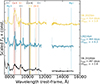 |
Fig. 35. Late-time NIR spectra of SN 2018ibb and the slow-evolving SLSNe LSQ14an and SN 2015bn. The strongest features are labelled. SN 2018ibb is the only SLSN that shows cobalt in emission, which has its strongest optical-NIR feature at 1.025 μm. Its luminosity translates to a nickel mass of ≳30 M⊙, consistent with the light curve modelling. All spectra are scaled so that O Iλ 7773 has the same amplitude in all objects. Regions of strong atmospheric absorption are cropped. |
In conclusion, SN 2018ibb is spectroscopically similar to other SLSNe, including slow-evolving SLSNe. During the photospheric phase, SN 2018ibb stands out by its low ejecta velocity and flat velocity evolution. The early nebular phase does not differ from other SLSNe. Very late-time observations (t/tdecline > 5) show clear differences between SN 2018ibb and other SLSNe, for example, the weak and broad [O I] that stays optically thick throughout the entire evolution. Late-time NIR spectroscopy revealed the tentative detection of [Co II] in SN 2018ibb. This feature is unprecedented for a SLSN and could be the smoking gun that SN 2018ibb is powered by the decay of 56Ni. In Sects. 4.3.3, 5.1, 4.3.4 and 5.2.4, we argued that the blue pseudo-continuum in SN 2018ibb is produced by the interaction of the SN ejecta with CSM. The prevalence of this feature in the other slow-evolving SLSNe raises the question of whether CSM interaction is also present in these objects. If this is the case, it is necessary to treat nebular spectra of SLSNe as the sum of at least two powering mechanisms, for example, magnetar + CSM or 56Ni + CSM, necessitating more complex SLSN models than the ones that currently exist. This also means that distinguishing between different powering mechanisms is more difficult and requires comprehensive data sets.
5.5. Is SN 2018ibb a pair-instability supernova?
Models of H-poor PISNe make very clear predictions for PISNe in the regime of SLSNe (Mpeak ≲ −20 mag) for their light curves (Kasen et al. 2011; Dessart et al. 2013; Gilmer et al. 2017; Kozyreva et al. 2017), ejecta velocities, spectra (Dessart et al. 2013; Jerkstrand et al. 2016) and the environments in which their progenitors are formed (Langer et al. 2007). In Sects. 4.6 and 5.2, we tested the most critical predictions of the PISN models on the light curves, spectra and host galaxy. SN 2018ibb passes most tests of PISN models with a nickel yield of 25–44 M⊙. However, SN 2018ibb did not comply with two predictions, although it could pass these tests with the interpretations that we propose. Table 11 summarises all tests.
Summary of the PISN tests applied on SN 2018ibb.
The tentative detection of [Co II] λ 1.025 μm is unprecedented for a PISN candidate. However, existing PISN models do not predict significant emission from [Co II] because of line blocking. In Sect. 5.2.5, we proposed that line blocking could be less severe than predicted by existing models.
The shape and the relative line intensities of the nebular spectra of SN 2018ibb are compatible with those predicted by PISN models. Our observations reveal a significant excess at wavelengths shorter than 5000 Å, which should not be present if 25–44 M⊙ of iron group elements were formed. As we concluded in Sect. 5.2.4, we propose that CSM interaction may account for some, if not all, of the excess. PISN models consider mass loss (Kasen et al. 2011; Gilmer et al. 2017; Kozyreva et al. 2017; Dessart et al. 2013) in the evolution of the progenitor star. However, their light curves and spectra are computed assuming that any interaction between the SN ejecta and the circumstellar material is negligible. Kasen et al. (2011) pointed out that the CSM interaction could actually have a non-negligible contribution. Furthermore, the CSM might not only be produced by stellar winds but also by eruptions similar to that seen in Eta Carinae in 1843. That this is indeed a non-negligible effect is corroborated by recent findings in Chen et al. (2023a). These authors studied the light curves of 77 events from the homogenous ZTF SLSN-I sample, and concluded that CSM is common around H-poor SLSNe (in at least 25–44% of the events) and that it contributes to the observed emission, albeit finding spectroscopic evidence in the spectra is difficult. Owing to the lack of predictions of PISN models on CSM interaction, we cannot firmly conclude that SN 2018ibb is a PISN.
Our observations demonstrate that interactions between the SN ejecta and the ambient CSM play a non-negligible effect in the observed photometric and spectroscopic properties (Sects. 4.3.3, 4.3.4, 5.1, 5.2.4). PISN models of H-poor progenitors with CSM are urgently needed. In the coming years, the Rubin Observatory, and the James Webb, Euclid and Roman Space Telescopes will systematically explore the high-redshift Universe. Since PISNe require metal-poor stars and the early Universe was less chemically enriched than today, PISNe are thought to be more abundant at higher redshifts. Several teams have proposed search strategies to find PISNe with these new observing facilities (e.g. Wang et al. 2017; Regős et al. 2020; Moriya et al. 2022a,b). However, their search strategies are based on PISN models that, for instance, do not include CSM interaction. Considering that these new observing facilities either just started or will commence their science operations in the next years, it is critical to expand the suite of existing PISN models in order to find high-z PISNe in real-time.
5.6. Could SN 2018ibb be a pulsational pair-instability supernova?
The massive eruptions in a pulsational pair-instability supernova (PPISN) with a large kinetic energy can, under the right conditions, be an ideal case for a luminous interacting SN, as demonstrated in several studies (e.g. Woosley et al. 2007; Yoshida et al. 2016; Woosley 2017; Leung et al. 2019; Marchant et al. 2019; Renzo et al. 2020). While the PPI mechanism is difficult to avoid for a He core in the mass range of 40–65 M⊙ (Woosley et al. 2007), the number of pulses and the interval between these, as well as the mass ejected and their kinetic energies, are more uncertain and differ between various studies. For a bright event to take place, the relative velocities between the shells of the different ejections, as well as their relative masses are important. The brightest event would result from the collision between a very fast, massive shell and a shell of low or zero velocity. The first shell must also be dense enough for the shocks to be radiative and massive enough for the second shell to be completely decelerated. Finally, the collision has to take place close enough to the star, on the order of 1015 − 1016 cm, so that it will radiate the energy on a timescale of approximately a year. This means that the interval between the pulses should not be more than approximately a year. However, a collision at a very small radius, and short time interval, will result in a very optically thick shell where most of the released energy will go into adiabatic expansion. In summary, there are a number of conditions which have to be fulfilled for a bright SN to result. This has been illustrated in detail by the different radiation-hydrodynamical models, for example, Woosley (2017).
Below, we discuss the most extreme models in order to judge whether a pure PPISN could explain the large total radiated energy we find for SN 2018ibb. For a pure He core, Woosley (2017) finds an upper limit to the kinetic energy of ∼2 × 1051 erg, with the highest energy from the highest He core mass, if no additional power source (e.g. magnetar or black hole accretion) is involved. The most extreme model with a 62 M⊙ He core resulted in a 36 M⊙ ejecta with a total kinetic energy of 2.1 × 1051 erg. This is distributed over several pulses, with most of the energy being dissipated in the first pulse. Without any previous strong mass loss this will, however, not be converted into radiation over a timescale of approximately a year. This is also confirmed by the light curve models in Woosley (2017).
Brighter light curves could be obtained for models with a remaining hydrogen envelope. The most extreme, T130D in Woosley (2017), had three pulses, ejecting the 70 M⊙ hydrogen-rich envelope with a kinetic energy of 1.5 × 1051 erg. About 3300 yr later a second pulse ejected a 7.7 M⊙ shell with He, C and O and energy 1.1 × 1051 erg, and after another 8 months a 13.5 M⊙ shell and energy 1.5 × 1051 erg. The last two shells were ejected close enough in time to collide and create a luminous SN with a total radiated energy of 4.5 × 1050 erg.
Similar calculations have been done by Marchant et al. (2019) and Leung et al. (2019), using the MESA code (while Woosley 2017 used the KEPLER code). Qualitatively, these models agree, especially in the higher energies and mass ejected, as well as the number of pulses with increasing He core mass. In particular, Leung et al. (2020) find a maximum kinetic energy of 2.8 × 1051 erg for the highest PPI He core mass, similar to the corresponding model by Woosley et al. (2007). However, as discussed by Leung et al. (2019), there are also substantial quantitative differences between the models, including ejected masses and time interval between the pulses. Some of the differences can be traced back to the treatment of shocks, and convection in both the hydrostatic and hydrodynamic phases.
We note that a large kinetic energy in PPISN models has also been invoked to explain the light curves of other luminous SNe. For the FBOT AT2018cow, Leung et al. (2020) invoked a kinetic energy of 5 × 1051 erg from a 42 M⊙ He-core interacting with an ejected shell with mass of 0.5 M⊙. An obvious solution to supply the extra energy is a hybrid model with a combination of a PPISN and the energy from a magnetar or accretion. This has been discussed by Woosley (2017) and for other energetic SLSNe including PTF12dam (Tolstov et al. 2017a), Gaia16apd (Tolstov et al. 2017b) and iPTF16eh (Lunnan et al. 2018a). However, it remains unclear how a magnetar can be formed from the core collapse of the very massive He core in a PPISN.
In summary, a pure PPISN, close to the upper He core mass limit, may potentially explain the observed radiated energy of > 3 × 1051 erg (Sect. 4.2.2). The conversion of kinetic energy to radiative energy, however, requires rather special conditions in terms of pulse intervals, ejecta mass and velocities. The uncertainties in the models are, unfortunately, large, and it is difficult to draw any firm conclusions. Additional energy sources can not be excluded, such as a magnetar or a black hole. A contribution from a magnetar would result in the flattening of the late-time light curve which is in stark contrast to our observations. In the case a black hole was formed during the gravitational collapse of the progenitor star, the accretion rate would need to be well-tuned to be consistent with the exponentially declining light curve, making the PPISN scenario less likely.
5.7. PISN rate constraint
Assuming that SN 2018ibb is a genuine PISN and that the PISN and SLSN luminosity functions are roughly the same, we can measure the PISN rate as a function of SLSNe. As of 25 July 2023, the spectroscopically complete ZTF Bright Transient Survey (BTS; Fremling et al. 2020; Perley et al. 2020) includes 24 genuine SLSNe-I with an absolute peak magnitude of < − 21 mag and an apparent peak magnitude of < 19 mag28. None of these objects are photometrically similar to SN 2018ibb. Using Binomial statistics, we place an upper limit of 14% (2σ confidence) on the PISN-to-SLSN rate. The latest version of the BTS catalogue reports a volumetric SLSN-I rate of 5 ± 2 Gpc−3 yr−1 between z = 0.1 and z = 0.2 (Perley priv. comm.). This translates the PISN-to-SLSN rate to a volumetric rate of < 0.7 yr−1 Gpc−3 in the same redshift interval (2σ confidence).
With a peak magnitude of r ∼ 17.7 mag (Table 5), SN 2018ibb passes the brightness cut of the BTS survey. However, it failed the BTS quality cuts as it contaminated all ZTF reference images. Assuming that SN 2018ibb would have passed the BTS quality cuts, we can place a lower limit on the volumetric rate. Following the methodology in Perley et al. (2020), the volumetric rate is
where N is the number of events, T is the BTS survey duration of 4.9 yr, DL is the maximum distance at which a transient with a given magnitude can be detected, fsky is the average nightly BTS sky coverage of 35%, and fretention is the retention factor (= 1, as SN 2018ibb is assumed to be detected). For N and DL, we apply the following considerations. Firstly, a Poisson distribution with a mean of 1 (= one PISN detection in the entire survey) has a lower 2σ confidence interval of 0.025 objects (Gehrels 1986). Secondly, at the BTS completeness limit of 18.5 mag, SN 2018ibb would have been detected up to a distance of 0.8 Gpc which we assume for DL. This yields a lower limit of > 9 × 10⁻³ yr−1 Gpc−3 at 2σ confidence (i.e. 0.2% of the SLSN rate).
Expected PISN rates vary between 10−5 and 10−2 of the core-collapse supernova rate (e.g. Langer et al. 2007; Briel et al. 2022). They are very sensitive to the assumed shape of the IMF, the metallicity of the progenitor star (Langer et al. 2007), stellar evolution models (e.g. nuclear reaction rates, rotation, mixing, mass-loss history; Takahashi 2018; du Buisson et al. 2020; Farmer et al. 2020), the cosmic star-formation history (Briel et al. 2022), redshift (Langer et al. 2007; Briel et al. 2022), and whether the progenitor system evolves as an isolated object or in a binary system (Briel et al. 2022; Tanikawa et al. 2023). This precludes a detailed comparison of the observed and expected rates. Our rate measurement of 0.009–0.7 yr−1 Gpc−3 is significantly smaller than all but one prediction. Briel et al. (2022) computed the PISN rate using various prescriptions for the cosmic star-formation history. For one of the prescriptions, these authors deduced a rate of ∼0.8 yr−1 Gpc−3, comparable with our upper limit of < 0.7 yr−1 Gpc−3. A more in-depth comparison is beyond the scope of this paper.
6. Conclusion
In this paper, we have presented observations of the slow-evolving H-poor SLSN 2018ibb covering an exceptionally long time interval from −93 to +989 rest-frame days after maximum. SN 2018ibb shares many similarities with H-poor SLSNe, but its properties are extreme even for SLSNe. It is one of the slowest evolving SLSNe known. The slow evolution is apparent through the long rise of > 93 rest-frame days from 10% peak flux to peak, the slow decline of merely 1.1 mag (100 days)−1, and the low photospheric velocity of 8500 km s−1 that remains constant between the time of maximum and the following 100 rest-frame days. At peak, SN 2018ibb reached an absolute magnitude of Mr = −21.7 mag, comparable to the bulk of the SLSN population. The bolometric light curve had a peak luminosity of > 2 × 1044 erg s−1. During its lifetime, SN 2018ibb radiated > 3 × 1051 erg. The peak luminosity and total radiated energy are strict lower limits.
We compared SN 2018ibb with PISN and SLSN models. SN 2018ibb complies with most tests of PISN models with peak luminosity < − 20 mag, and possibly all tests with the interpretations that we propose, making SN 2018ibb the best PISN candidate, to date. Specifically, SN 2018ibb passes the following tests:
-
(i)
a rise time of > 93 days (expected: 120–150 days)
-
(ii)
a decline time scale of 1.1 mag (100 days)−1 (expected: 1.1 mag (100 days)−1)
-
(iii)
the modelling of the multi-band light curves with physical SLSN models and the Katz et al. (2013) method point to the production of 25–
 Ni (expected: 10–44 M⊙)
 -
(iv)
the bolometric light curve is consistent with PISN templates that produce 25 and 44 M⊙ of 56Ni
-
(v)
a low ejecta velocity of 8500 km s−1 (expected: 7000–11 000 km s−1)
-
(vi)
a flat evolution of the velocity after maximum light during the photospheric phase (expected: flat evolution)
-
(vii)
a low metallicity of ∼0.25 solar (expected: < 1/3 solar)
-
(viii)
none of the > 200 SLSNe has properties similar to SN 2018ibb (expected: PISNe are rare).
Such a huge amount of nickel of 25–44 M⊙ can only be produced in a pair-instability-supernova explosion of a star with a He-core mass of 120–130 M⊙ at the time of the explosion (ZAMS mass of approximately 240–260 M⊙). However, SN 2018ibb does not comply with the following tests:
-
(i)
the tentative detection of [Co II] λ 1.025 μm in emission, implying M(56Ni)≳30 M⊙ (expected: no [Co II] in emission)
-
(ii)
the nebular spectra are similar to the He130 [M(56Ni)=44 M⊙] PISN model but show a substantial excess bluewards of 5000 Å due to CSM interaction.
The tentative detection of [Co II] is unprecedented for a PISN candidate and any SLSN. It could be the smoking-gun evidence of SN 2018ibb being a PISN, though the line identification hinges on the detection of a single line. PISN models predict no significant [Co II] λ 1.025 μm in emission because of line blocking extending by iron to the NIR. We propose that the line blocking might be over-estimated in existing models.
While the late-time spectra are similar to PISN models, they also exhibit a blue excess that should not be present due to the massive line-blanketing of 25–44 M⊙ iron-group elements. A similar blue excess was also observed in previous PISN candidates. Its presence was used as a critical piece of evidence against the PISN interpretation. We argue that this is not the case for SN 2018ibb. Three lines of evidence reveal that SN 2018ibb is not solely powered by radioactivity and that CSM interaction is also at play: (i) the detection of a slow-moving CSM shell around the progenitor star; (ii) the presence of similarly slow O I, [O II], [O III] emission lines; and (iii) a blue pseudo-continuum similar to that of interaction-powered SNe. This suggests that some, if not all, of the blue excess is produced by CSM interaction. We stress that even after accounting for a substantial contribution of CSM interaction to the bolometric flux, 25–44 M⊙ are still required to power the entire bolometric light curve.
PISN models consider mass-loss episodes (winds and to some level eruptions) to evolve their progenitors to the point of explosion. However, the SN light curves and spectra are computed in sterile environments, assuming that any interaction between the SN ejecta and the circumstellar material is negligible. Our observations demonstrate that CSM interaction is an important non-negligible effect that needs to be systematically explored in PISN models. The lack of such PISN models is the reason why we cannot conclusively argue for SN 2018ibb being a PISN.
Our data set disfavours central engine models (magnetar powering and fallback accretion onto a black hole), the magnetar+56Ni model and pure CSM models. The continued linear decline out to tmax+706 days and the absence of any light curve flattening, expected for magnetar models, are in conflict with existing analytical prescriptions of magnetar models. Furthermore, the inferred values of the physical parameters of the magnetar and magnetar+56Ni models are in conflict with existing stellar evolution models. A model with a simple-power-law-shaped fallback accretion rate, the default assumption in fallback models, would also result in a flattening of the light curve in contradiction with our observations. Analytical CSM models did not provide an adequate description either.
The extensive, high-quality dataset of SN 2018ibb is predestined to perform definitive tests with SLSN and PISN models, and to explore rare explosion mechanisms, such as axion-instability supernovae (AISNe; Sakstein et al. 2022). Simulations by Mori et al. (2023) suggest that AISNe evolve faster and are bluer than PISNe for a given He-core mass. AISNe might also be more abundant than PISNe. Therefore, revealing the powering mechanism of SN 2018ibb will have immediate consequences not only for SN science but also for stellar evolution theory. The final confirmation of a PISN would also have ramifications for the interpretation of the observed drop in the black hole mass function and, therefore, gravitational wave astronomy.
In the coming years, the Rubin Observatory, and the James Webb, Euclid and Roman Space Telescopes will be used to search for SLSNe, PISNe, and the explosions of Population III stars in the high-redshift Universe. To make this leap forward, the community requires a significantly improved understanding of the powering mechanisms and the progenitors of SLSNe. This can be accomplished with (i) comprehensive data sets of low-z SLSNe similar to the one presented here and (ii) more complex theoretical models with clear predictions for light curves and spectra. The James Webb Space Telescope could be transformative for studying low-redshift SLSNe. Its IR spectrograph NIRspec has the sensitivity to provide an uncensored view from 1 to 5 μm. Such an IR spectrum of a SN 2018ibb-like event could reveal strong emission lines from cobalt, nickel and iron between 2 and 5 μm during the nebular phase29, which would be the smoking-gun30 evidence for powering by 56Ni.
The GROND, ZTF and EFOSC2 g-band filters have an effective wavelength of 4504, 4723, 5104 Å and width of 1373, 1282, 788 Å, respectively (retrieved from the Spanish Virtual; Rodrigo et al. 2012, and references therein).
The photon index is defined as the power-law index of the photon flux density (N(E)∝E−Γ).
The host extinction is negligible (Sect. 4.6).
The last ATLAS non-detection is from 17 August 2018, that is, 1.3 rest-frame days after the first Gaia detection, reaching a limiting magnitude of o ≈ 19.9 mag at 3σ confidence.
The Gaia alert database reports an observation on 5 July 2018 but no measurement. This could either mean (i) a non-detection (limiting magnitude G = 20.7 mag) and hence imposing an upper limit of < 129 days on t1/10, rise, (ii) the observation was not performed, or (iii) a problem in the data processing (Hodgkin et al. 2021).
We added a systematic error of 5% to all optical and NIR filters and 10% to all UV filters in quadrature to account for uncertainties in the flux calibration.
Based on the correlations between the stellar mass of galaxies and the width of galaxy absorption and emission lines (Krühler et al. 2015; Arabsalmani et al. 2018).
PTF10hgi was detected in the radio > 7.5 yr after the SN explosion. Owing to this, we omit to show PTF10hgi in that figure.
PROSPECTOR uses the FLEXIBLE STELLAR POPULATION SYNTHESIS (FSPS) code (Conroy et al. 2009) to generate the underlying physical model and PYTHON-FSPS (Foreman-Mackey et al. 2014) to interface with FSPS in PYTHON. The FSPS code also accounts for the contribution from the diffuse gas based on the CLOUDY models from Byler et al. (2017). We use the dynamic nested sampling package DYNESTY (Speagle 2020) to sample the posterior probability.
Type Ia supernovae are a class of supernovae that occurs in binary systems in which one of the stars is a white dwarf (e.g. Hillebrandt & Niemeyer 2000, and references therein). This explosion produces ∼0.6 M⊙ of 56Ni (e.g. Maoz et al. 2014, and references therein).
All measurements are based on the fiducial assumption of dipole spin-down radiation. For a discussion on the impact of non-dipole radiation see Omand & Sarin (2024).
The model spectra of the P250 templates will be presented in a forthcoming paper by Kozyreva et al. (in prep.).
The pseudo-continuum in Type Ibn SNe is the product of the blending of thousands of iron emission lines (e.g. Dessart et al. 2022).
Using spectra of Type Ia-CSM or Ibn SNe would give similar results. We decided to use an Icn template because it shows no emission lines from H and He, which are present in Type Ia-CSM and Ibn SNe.
This feature consists of six lines between 1.0287 and 1.0370 μm.
The ZTF-I SLSN sample contains a further possible slow-evolving SLSN. SN 2018lzx has a rise ( days) and a decline (
 days) time scale comparable to SN 2018ibb (Table 5). The peak absolute magnitude is 0.2 mag brighter than that of SN 2018ibb (Chen et al. 2023b). Owing to its high redshift of z = 0.44, the light curve spans a short time interval before SN 2018lxz faded below the detection threshold, and the quality of the spectra is significantly lower compared to that of SN 2018ibb. Therefore, we exclude this SLSN from the comparison.
Owing to the high redshift of PS1-11ap and PS1-14bj, we use their i-band light curves, which probe a rest-frame wavelength interval similar to that of the g band of SN 2018ibb.
LSQ14an is omitted from this comparison. Conspicuous galaxy lines from [O III] λλ 4959,5007 contaminate the Fe IIλ 5169 region.
The BTS has a spectroscopic completeness of 95% down to m = 18.5 mag (https://sites.astro.caltech.edu/ztf/bts/explorer.php). Although, the completeness is lower at m = 19, we can go down to that fainter magnitude limit to get a minimum number of spectroscopically confirmed SLSNe and place an upper limit on the PISN-to-SLSN rate.
https://gist.github.com/thespacedoctor/gi86777fa5a9567b7939e8d84fd8cf6a76
Acknowledgments
We thank the referee for a careful reading of the manuscript and for helpful comments that improved this paper. We thank Stéphane Blondin (Laboratoire d’Astrophysique de Marseille, France), Luc Dessart (Sorbonne Université, France), Sebastian Gomez (Space Telescope Science Institute, USA), Ryosuke Hirai (Monash University, Australia), Boaz Katz (Weizmann Institute of Science, Israel), Keiichi Maeda (Kyoto University, Japan), Ilya Mandel (Monash University, Australia), and Kanji Mori (Fukuoka University, Japan) for fruitful discussions. U.C. Berkeley undergraduate students Nachiket Girish, Andrew Hoffman, Evelyn Liu, Shaunak Modak, Jackson Sipple, Samantha Stegman, Kevin Tang, and Keto Zhang helped obtain data with the Lick/Nickel telescope. Z. C. acknowledges support from the China Scholarship Council. A. V. Filippenko’s supernova group at U.C. Berkeley received financial support from the Christopher R. Redlich Fund, Gary & Cynthia Bengier, Clark & Sharon Winslow, Sanford Robertson, Frank and Kathleen Wood (T. G. Brink is a Wood Specialist in Astronomy), Alan Eustace (W. Zheng is a Eustace Specialist in Astronomy), and numerous other donors. C. F. acknowledges support from the Swedish Research Council and the Swedish National Space Board. J. P. U. F. acknowledges support from the Carlsberg Foundation. The Cosmic Dawn Center (DAWN) is funded by the Danish National Research Foundation under grant No. 140. M. G. is supported by the EU Horizon 2020 research and innovation programme under grant agreement No. 101004719. A. J. acknowledges support from the European Research Council (ERC) under the European Union’s Horizon 2020 Research and Innovation Programme (ERC Starting Grant No. [803189]). H. K. was funded by the Academy of Finland projects 324504 and 328898. G. L. and M. P. are supported by a research grant (19054) from VILLUM FONDEN. R. L. is supported by the European Research Council (ERC) under the European Union’s Horizon Europe research and innovation programme (grant agreement No. 10104229 – TransPIre). T. E. M.-B. and L. G. acknowledge financial support from the Spanish Ministerio de Ciencia e Innovación (MCIN), the Agencia Estatal de Investigación (AEI) 10.13039/501100011033, the European Social Fund (ESF) “Investing in your future”, and the European Union Next Generation EU/PRTR funds under the PID2020-115253GA-I00 HOSTFLOWS project, the 2019 Ramón y Cajal program RYC2019-027683-I, the 2021 Juan de la Cierva program FJC2021-047124-I, and from Centro Superior de Investigaciones Científicas (CSIC) under the PIE project 20215AT016, and the program Unidad de Excelencia María de Maeztu CEX2020-001058-M. M. N. is supported by the European Research Council (ERC) under the European Union’s Horizon 2020 research and innovation programme (grant agreement No. 948381) and by a Fellowship from the Alan Turing Institute. D. P. is grateful for the Wise Observatory staff. A. R. acknowledges support from Premiale LBT 2013. M. R. has received funding from the European Research Council (ERC) under the European Union’s Horizon 2020 research and innovation programme (grant agreement No. 759194 – USNAC). N. S. is supported by a Nordita Fellowship. Nordita is funded in part by NordForsk. S. S. acknowledges support from the G.R.E.A.T. research environment, funded by Vetenskapsrådet, the Swedish Research Council, project number 2016-06012. L. J. S. acknowledges support by the European Research Council (ERC) under the European Union’s Horizon 2020 research and innovation program (ERC Advanced Grant KILONOVA No. 885281). L. T. acknowledges support from MIUR (PRIN 2017 grant 20179ZF5KS). Y. Y. acknowledges support from a Benoziyo Prize Postdoctoral Fellowship and the Bengier-Winslow-Robertson Fellowship. This work was funded by ANID, Millennium Science Initiative, ICN12_009. Based in part on observations at the European Southern Observatory, Program IDs 199.D-0143, 0105.D-0380, 0106.D-0524, 1103.D-0328, 2102.D-5026, and 2104.D-5006 (PIs C. Inserra, S. Schulze, and S. J. Smartt); Gemini-South, Program ID 2021B-Q-901 (PI A. Gal-Yam); Hubble Space Telescope, Program ID GO-16657 (PI C. Fremling); Keck, Program IDs C323, U023, U025 (PIs S. R. Kulkarni, A. V. Filippenko); Large Binocular Telescope, Program ID DDT_2019B_13 (PI E. Palazzi); Las Cumbres Observatory, Program IDs FTPEPO2017AB-001, KEY2017AB-001, SUPA2019A-001, SUPA2019A-002, SUPA2019B-007, and NOAO2020B-012 (PIs P. J. Brown, K. De); Liverpool Telescope, Program IDs JL18B06, JL18B07, JL19A24, JL19B11, and JL20B15 (PI D. A. Perley); Nordic Optical Telescope, Program IDs 57-502, 58-802, and 61-606, (PIs G. Leloudas, J. Sollerman); P200 (PI L. Yan); and XMM-Newton, Program ID 08221501 (PI R. Margutti). We thank the staffs of the many observatories at which we conducted observations. This work has made use of data from the European Space Agency (ESA) mission Gaia, processed by the Gaia Data Processing and Analysis Consortium (DPAC). Funding for the DPAC has been provided by national institutions, in particular the institutions participating in the Gaia Multilateral Agreement. Part of the funding for GROND (both hardware as well as personnel) was generously granted from the Leibniz-Prize to Prof. G. Hasinger (DFG grant HA 1850/28-1). This work is based in part on observations made with the Large Binocular Telescope (LBT). The LBT is an international collaboration among institutions in Italy, the United States, and Germany. LBT Corporation partners are Istituto Nazionale di Astrofisica, Italy; The University of Arizona on behalf of the Arizona university system; LBT Beteiligungsgesellschaft, Germany, representing the Max Planck Society, the Astrophysical Institute Potsdam, and Heidelberg University; The Ohio State University; and The Research Corporation on behalf of The University of Notre Dame, University of Minnesota, and University of Virginia. Some of the observations with the Las Cumbres Observatory data have been obtained via OPTICON proposals and as part of the Global Supernova Project. The OPTICON project has received funding from the European Union’s Horizon 2020 research and innovation programme under grant agreement No. 730890. This work made use of data supplied by the UK Swift Science Data Centre at the University of Leicester. CRTS is supported by the U.S. National Science Foundation (NSF) under grants AST-0909182, AST-1313422, and AST-1413600. The Catalina Sky Survey (CSS) is a NASA-funded project supported by the Near Earth Object Observation Program (NEOO) under the Planetary Defense Coordination Office (PDCO). This publication makes use of data products from the Two Micron All Sky Survey, which is a joint project of the University of Massachusetts and the Infrared Processing and Analysis Center/California Institute of Technology, funded by NASA and the U.S. NSF. Based in part on observations obtained with the Samuel Oschin Telescope 48-inch and the 60-inch Telescope at the Palomar Observatory as part of the Zwicky Transient Facility project. ZTF is supported by the U.S. NSF under grant AST-1440341 and a collaboration including Caltech, IPAC, the Weizmann Institute of Science, the Oskar Klein Center at Stockholm University, the University of Maryland, the University of Washington, Deutsches Elektronen-Synchrotron and Humboldt University, Los Alamos National Laboratories, the TANGO Consortium of Taiwan, the University of Wisconsin at Milwaukee, and Lawrence Berkeley National Laboratories. Operations are conducted by COO, IPAC, and UW. The SED Machine is based upon work supported by the U.S. NSF under grant 1106171. Partially based on observations made with the Nordic Optical Telescope, owned in collaboration by the University of Turku and Aarhus University, and operated jointly by Aarhus University, the University of Turku and the University of Oslo, representing Denmark, Finland and Norway, the University of Iceland and Stockholm University at the Observatorio del Roque de los Muchachos, La Palma, Spain, of the Instituto de Astrofisica de Canarias. This work makes use of observations from the Las Cumbres Observatory network. The Las Cumbres Observatory team is supported by NSF grants AST-1911225 and AST-1911151. Some of the data presented herein were obtained at the W. M. Keck Observatory, which is operated as a scientific partnership among the California Institute of Technology, the University of California, and NASA; the observatory was made possible by the generous financial support of the W. M. Keck Foundation. KAIT, and its ongoing operation were made possible by donations from Sun Microsystems, Inc., the Hewlett-Packard Company, AutoScope Corporation, the Lick Observatory, the U.S. NSF, the University of California, the Sylvia & Jim Katzman Foundation, and the TABASGO Foundation. A major upgrade of the Kast spectrograph on the Shane 3 m telescope at Lick Observatory was made possible through generous gifts from William and Marina Kast as well as the Heising-Simons Foundation. Research at Lick Observatory is partially supported by a generous gift from Google.
References
- Ageorges, N., Seifert, W., Jütte, M., et al. 2010, SPIE Conf. Ser., 7735, 77351L [Google Scholar]
- Ambikasaran, S., Foreman-Mackey, D., Greengard, L., Hogg, D. W., & O’Neil, M. 2015, IEEE Trans. Pattern Anal. Mach. Intell., 38, 252 [Google Scholar]
- Anderson, J., Mieske, S., & Kaufer, A. 2018, European Southern Observatory, Doc. No. VLT-MAN-ESO-13100-1543 [Google Scholar]
- Andrews, B. H., & Martini, P. 2013, ApJ, 765, 140 [NASA ADS] [CrossRef] [Google Scholar]
- Angus, C. R., Smith, M., Sullivan, M., et al. 2019, MNRAS, 487, 2215 [NASA ADS] [CrossRef] [Google Scholar]
- Aoki, W., Tominaga, N., Beers, T. C., Honda, S., & Lee, Y. S. 2014, Science, 345, 912 [NASA ADS] [CrossRef] [Google Scholar]
- Appenzeller, I., Fricke, K., Fürtig, W., et al. 1998, Messenger, 94, 1 [Google Scholar]
- Arabsalmani, M., Møller, P., Perley, D. A., et al. 2018, MNRAS, 473, 3312 [NASA ADS] [CrossRef] [Google Scholar]
- Ashton, G., Hübner, M., Lasky, P. D., et al. 2019, ApJS, 241, 27 [NASA ADS] [CrossRef] [Google Scholar]
- Asplund, M., Grevesse, N., Sauval, A. J., & Scott, P. 2009, ARA&A, 47, 481 [NASA ADS] [CrossRef] [Google Scholar]
- Barkat, Z., Rakavy, G., & Sack, N. 1967, Phys. Rev. Lett., 18, 379 [Google Scholar]
- Bauer, F. E., Dwarkadas, V. V., Brandt, W. N., et al. 2008, ApJ, 688, 1210 [NASA ADS] [CrossRef] [Google Scholar]
- Becker, A. 2015, Astrophysics Source Code Library [record ascl:1504.004] [Google Scholar]
- Belczynski, K., Klencki, J., Fields, C. E., et al. 2020, A&A, 636, A104 [NASA ADS] [CrossRef] [EDP Sciences] [Google Scholar]
- Bellm, E. C., Kulkarni, S. R., Graham, M. J., et al. 2019a, PASP, 131, 018002 [Google Scholar]
- Bellm, E. C., Kulkarni, S. R., Barlow, T., et al. 2019b, PASP, 131, 068003 [Google Scholar]
- Ben-Ami, S., Gal-Yam, A., Mazzali, P. A., et al. 2014, ApJ, 785, 37 [NASA ADS] [CrossRef] [Google Scholar]
- Bertin, E. 2012, ASP Conf. Ser., 461, 263 [Google Scholar]
- Bertin, E., & Arnouts, S. 1996, A&AS, 117, 393 [NASA ADS] [CrossRef] [EDP Sciences] [Google Scholar]
- Blagorodnova, N., Neill, J. D., Walters, R., et al. 2018, PASP, 130, 035003 [Google Scholar]
- Blanchard, P. K., Nicholl, M., Berger, E., et al. 2019, ApJ, 872, 90 [NASA ADS] [CrossRef] [Google Scholar]
- Blanchard, P. K., Berger, E., Nicholl, M., & Villar, V. A. 2020, ApJ, 897, 114 [NASA ADS] [CrossRef] [Google Scholar]
- Blanton, M. R., & Roweis, S. 2007, AJ, 133, 734 [NASA ADS] [CrossRef] [Google Scholar]
- Blinnikov, S. I., & Sorokina, E. I. 2010, arXiv e-prints [arXiv:1009.4353] [Google Scholar]
- Blinnikov, S. I., Röpke, F. K., Sorokina, E. I., et al. 2006, A&A, 453, 229 [NASA ADS] [CrossRef] [EDP Sciences] [Google Scholar]
- Bradley, L., Sipőcz, B., Robitaille, T., et al. 2020, https://doi.org/10.5281/zenodo.4044744 [Google Scholar]
- Branch, D., Baron, E., Hall, N., Melakayil, M., & Parrent, J. 2005, PASP, 117, 545 [NASA ADS] [CrossRef] [Google Scholar]
- Brands, S. A., de Koter, A., Bestenlehner, J. M., et al. 2022, A&A, 663, A36 [Google Scholar]
- Breeveld, A. A., Landsman, W., Holland, S. T., et al. 2011, AIP Conf. Ser., 1358, 373 [Google Scholar]
- Briel, M. M., Eldridge, J. J., Stanway, E. R., Stevance, H. F., & Chrimes, A. A. 2022, MNRAS, 514, 1315 [NASA ADS] [CrossRef] [Google Scholar]
- Bromm, V., & Larson, R. B. 2004, ARA&A, 42, 79 [NASA ADS] [CrossRef] [Google Scholar]
- Burrows, D. N., Hill, J. E., Nousek, J. A., et al. 2005, Space Sci. Rev., 120, 165 [Google Scholar]
- Buzzoni, B., Delabre, B., Dekker, H., et al. 1984, Messenger, 38, 9 [Google Scholar]
- Byler, N., Dalcanton, J. J., Conroy, C., & Johnson, B. D. 2017, ApJ, 840, 44 [Google Scholar]
- Calzetti, D., Armus, L., Bohlin, R. C., et al. 2000, ApJ, 533, 682 [NASA ADS] [CrossRef] [Google Scholar]
- Chabrier, G. 2003, PASP, 115, 763 [Google Scholar]
- Chambers, K. C., Magnier, E. A., Metcalfe, N., et al. 2016, arXiv e-prints [arXiv:1612.05560] [Google Scholar]
- Chandra, P., Chevalier, R. A., Chugai, N., et al. 2012, ApJ, 755, 110 [NASA ADS] [CrossRef] [Google Scholar]
- Chandra, P., Chevalier, R. A., Chugai, N., Fransson, C., & Soderberg, A. M. 2015, ApJ, 810, 32 [NASA ADS] [CrossRef] [Google Scholar]
- Chatzopoulos, E., & Wheeler, J. C. 2012, ApJ, 760, 154 [NASA ADS] [CrossRef] [Google Scholar]
- Chatzopoulos, E., Wheeler, J. C., & Vinko, J. 2012, ApJ, 746, 121 [Google Scholar]
- Chen, T.-W., Smartt, S. J., Bresolin, F., et al. 2013, ApJ, 763, L28 [NASA ADS] [CrossRef] [Google Scholar]
- Chen, T. W., Smartt, S. J., Jerkstrand, A., et al. 2015, MNRAS, 452, 1567 [NASA ADS] [CrossRef] [Google Scholar]
- Chen, T.-W., Smartt, S. J., Yates, R. M., et al. 2017, MNRAS, 470, 3566 [NASA ADS] [CrossRef] [Google Scholar]
- Chen, T. W., Inserra, C., Fraser, M., et al. 2018, ApJ, 867, L31 [NASA ADS] [CrossRef] [Google Scholar]
- Chen, K.-J., Woosley, S. E., & Whalen, D. J. 2020, ApJ, 897, 152 [NASA ADS] [CrossRef] [Google Scholar]
- Chen, Z. H., Yan, L., Kangas, T., et al. 2023a, ApJ, 943, 42 [NASA ADS] [CrossRef] [Google Scholar]
- Chen, Z. H., Yan, L., Kangas, T., et al. 2023b, ApJ, 943, 41 [NASA ADS] [CrossRef] [Google Scholar]
- Chevalier, R., & Blondin, J. M. 1995, ApJ, 444, 312 [NASA ADS] [CrossRef] [Google Scholar]
- Chevalier, R. A., & Fransson, C. 1992, ApJ, 395, 540 [NASA ADS] [CrossRef] [Google Scholar]
- Chevalier, R. A., & Fransson, C. 1994, ApJ, 420, 268 [NASA ADS] [CrossRef] [Google Scholar]
- Chevalier, R. A., & Fransson, C. 2017, in Handbook of Supernovae, eds. A. W. Alsabti, & P. Murdin (Springer International Publishing AG), 875 [CrossRef] [Google Scholar]
- Chornock, R., & Filippenko, A. V. 2008, AJ, 136, 2227 [NASA ADS] [CrossRef] [Google Scholar]
- Conroy, C., Gunn, J. E., & White, M. 2009, ApJ, 699, 486 [Google Scholar]
- Coppejans, D. L., Margutti, R., Guidorzi, C., et al. 2018, ApJ, 856, 56 [NASA ADS] [CrossRef] [Google Scholar]
- Coppejans, D. L., Matthews, D., Margutti, R., et al. 2021, TNSAN, 73, 1 [NASA ADS] [Google Scholar]
- Corsi, A., Ofek, E. O., Gal-Yam, A., et al. 2014, ApJ, 782, 42 [NASA ADS] [CrossRef] [Google Scholar]
- Crowther, P. A. 2007, ARA&A, 45, 177 [Google Scholar]
- Dark Energy Survey Collaboration (Abbott, T., et al.) 2016, MNRAS, 460, 1270 [Google Scholar]
- De Cia, A., Gal-Yam, A., Rubin, A., et al. 2018, ApJ, 860, 100 [NASA ADS] [CrossRef] [Google Scholar]
- de Ugarte Postigo, A., Fynbo, J. P. U., Thöne, C. C., et al. 2012, A&A, 548, A11 [NASA ADS] [CrossRef] [EDP Sciences] [Google Scholar]
- Dekany, R., Smith, R. M., Riddle, R., et al. 2020, PASP, 132, 038001 [NASA ADS] [CrossRef] [Google Scholar]
- Dessart, L., & Audit, E. 2018, A&A, 613, A5 [Google Scholar]
- Dessart, L., & Hillier, D. J. 2005, A&A, 439, 671 [NASA ADS] [CrossRef] [EDP Sciences] [Google Scholar]
- Dessart, L., Waldman, R., Livne, E., Hillier, D. J., & Blondin, S. 2013, MNRAS, 428, 3227 [NASA ADS] [CrossRef] [Google Scholar]
- Dessart, L., Hillier, D. J., & Kuncarayakti, H. 2022, A&A, 658, A130 [NASA ADS] [CrossRef] [EDP Sciences] [Google Scholar]
- Dexter, J., & Kasen, D. 2013, ApJ, 772, 30 [NASA ADS] [CrossRef] [Google Scholar]
- Dey, A., Schlegel, D. J., Lang, D., et al. 2019, AJ, 157, 168 [Google Scholar]
- Drake, A. J., Djorgovski, S. G., Mahabal, A., et al. 2011, ApJ, 735, 106 [NASA ADS] [CrossRef] [Google Scholar]
- Drlica-Wagner, A., Sevilla-Noarbe, I., Rykoff, E. S., et al. 2018, ApJS, 235, 33 [Google Scholar]
- du Buisson, L., Marchant, P., Podsiadlowski, P., et al. 2020, MNRAS, 499, 5941 [Google Scholar]
- Eftekhari, T., Berger, E., Margalit, B., et al. 2019, ApJ, 876, L10 [NASA ADS] [CrossRef] [Google Scholar]
- Eftekhari, T., Margalit, B., Omand, C. M. B., et al. 2021, ApJ, 912, 21 [NASA ADS] [CrossRef] [Google Scholar]
- Ekström, S., Georgy, C., Eggenberger, P., et al. 2012, A&A, 537, A146 [Google Scholar]
- Elbaz, D., Daddi, E., Le Borgne, D., et al. 2007, A&A, 468, 33 [NASA ADS] [CrossRef] [EDP Sciences] [Google Scholar]
- Ellison, S. L., Ibata, R., Pettini, M., et al. 2004, A&A, 414, 79 [NASA ADS] [CrossRef] [EDP Sciences] [Google Scholar]
- Evans, P. A., Beardmore, A. P., Page, K. L., et al. 2007, A&A, 469, 379 [NASA ADS] [CrossRef] [EDP Sciences] [Google Scholar]
- Evans, P. A., Beardmore, A. P., Page, K. L., et al. 2009, MNRAS, 397, 1177 [Google Scholar]
- Farmer, R., Renzo, M., de Mink, S. E., Marchant, P., & Justham, S. 2019, ApJ, 887, 53 [Google Scholar]
- Farmer, R., Renzo, M., de Mink, S. E., Fishbach, M., & Justham, S. 2020, ApJ, 902, L36 [CrossRef] [Google Scholar]
- Fesen, R. A., Gerardy, C. L., Filippenko, A. V., et al. 1999, AJ, 117, 725 [NASA ADS] [CrossRef] [Google Scholar]
- Filippenko, A. V. 1982, PASP, 94, 715 [Google Scholar]
- Filippenko, A. V. 1997, ARA&A, 35, 309 [NASA ADS] [CrossRef] [Google Scholar]
- Filippenko, A. V., Li, W. D., Treffers, R. R., & Modjaz, M. 2001, ASP Conf. Ser., 246, 121 [NASA ADS] [Google Scholar]
- Finkbeiner, D. P., Schlafly, E. F., Schlegel, D. J., et al. 2016, ApJ, 822, 66 [Google Scholar]
- Fiore, A., Chen, T. W., Jerkstrand, A., et al. 2021, MNRAS, 502, 2120 [NASA ADS] [CrossRef] [Google Scholar]
- Foreman-Mackey, D., Sick, J., & Johnson, B. 2014, https://doi.org/10.5281/zenodo.12157 [Google Scholar]
- Fowler, W. A., & Hoyle, F. 1964, ApJS, 9, 201 [Google Scholar]
- Fransson, C. 1984, A&A, 132, 115 [NASA ADS] [Google Scholar]
- Fransson, C., Chevalier, R. A., Filippenko, A. V., et al. 2002, ApJ, 572, 350 [NASA ADS] [CrossRef] [Google Scholar]
- Fransson, C., Ergon, M., Challis, P. J., et al. 2014, ApJ, 797, 118 [Google Scholar]
- Fremling, C., Sollerman, J., Taddia, F., et al. 2016, A&A, 593, A68 [NASA ADS] [CrossRef] [EDP Sciences] [Google Scholar]
- Fremling, C., Dugas, A., & Sharma, Y. 2018a, TNS Classif. Rep., 2018-1877, 1 [Google Scholar]
- Fremling, C., Dugas, A., Sharma, Y., Yaron, O., & Gal-Yam, A. 2018b, TNS Classif. Rep., 2018-2180, 1 [Google Scholar]
- Fremling, C., Miller, A. A., Sharma, Y., et al. 2020, ApJ, 895, 32 [NASA ADS] [CrossRef] [Google Scholar]
- Fremling, C., Kasliwal, M., Sharma, Y., et al. 2021, Late-time NUV Snapshotsof the Lost Envelopes of Stripped Supernovae, HST Proposal. Cycle 29, ID. #16657 [Google Scholar]
- Fynbo, J. P. U., Jakobsson, P., Prochaska, J. X., et al. 2009, ApJS, 185, 526 [NASA ADS] [CrossRef] [Google Scholar]
- Gaia Collaboration (Prusti, T., et al.) 2016, A&A, 595, A1 [NASA ADS] [CrossRef] [EDP Sciences] [Google Scholar]
- Gal-Yam, A. 2012, Science, 337, 927 [Google Scholar]
- Gal-Yam, A. 2017, in Handbook of Supernovae, eds. A. W. Alsabti, & P. Murdin (Springer International Publishing AG), 195 [CrossRef] [Google Scholar]
- Gal-Yam, A. 2019a, ARA&A, 57, 305 [Google Scholar]
- Gal-Yam, A. 2019b, ApJ, 882, 102 [NASA ADS] [CrossRef] [Google Scholar]
- Gal-Yam, A., Mazzali, P., Ofek, E. O., et al. 2009, Nature, 462, 624 [NASA ADS] [CrossRef] [Google Scholar]
- Gal-Yam, A., Bruch, R., Schulze, S., et al. 2022, Nature, 601, 201 [NASA ADS] [CrossRef] [Google Scholar]
- Gehrels, N. 1986, ApJ, 303, 336 [Google Scholar]
- Gehrels, N., Chincarini, G., Giommi, P., et al. 2004, ApJ, 611, 1005 [Google Scholar]
- Gerosa, D., & Fishbach, M. 2021, Nat. Astron., 5, 749 [NASA ADS] [CrossRef] [Google Scholar]
- Gilkis, A., Soker, N., & Papish, O. 2016, ApJ, 826, 178 [NASA ADS] [CrossRef] [Google Scholar]
- Gilmer, M. S., Kozyreva, A., Hirschi, R., Fröhlich, C., & Yusof, N. 2017, ApJ, 846, 100 [NASA ADS] [CrossRef] [Google Scholar]
- Gimeno, G., Roth, K., Chiboucas, K., et al. 2016, SPIE Conf. Ser., 9908, 99082S [NASA ADS] [Google Scholar]
- Goldoni, P., Royer, F., François, P., et al. 2006, SPIE Conf. Ser., 6269, 62692K [Google Scholar]
- Gomez, S., Berger, E., Nicholl, M., et al. 2019, ApJ, 881, 87 [NASA ADS] [CrossRef] [Google Scholar]
- Graham, M. J., Kulkarni, S. R., Bellm, E. C., et al. 2019, PASP, 131, 078001 [Google Scholar]
- Greiner, J., Bornemann, W., Clemens, C., et al. 2008, PASP, 120, 405 [Google Scholar]
- Guillochon, J., Nicholl, M., Villar, V. A., et al. 2018, ApJS, 236, 6 [NASA ADS] [CrossRef] [Google Scholar]
- Hatano, K., Branch, D., Nomoto, K., et al. 2001, Am. Astron. Soc. Meet. Abstr., 198, 39.02 [NASA ADS] [Google Scholar]
- Heger, A., & Woosley, S. E. 2002, ApJ, 567, 532 [Google Scholar]
- Heger, A., Fryer, C. L., Woosley, S. E., Langer, N., & Hartmann, D. H. 2003, ApJ, 591, 288 [CrossRef] [Google Scholar]
- HI4PI Collaboration (Ben Bekhti, N., et al.) 2016, A&A, 594, A116 [NASA ADS] [CrossRef] [EDP Sciences] [Google Scholar]
- Hillebrandt, W., & Niemeyer, J. C. 2000, ARA&A, 38, 191 [Google Scholar]
- Hjorth, J., & Bloom, J. S. 2012, Camb. Astrophys. Ser., 51, 169 [NASA ADS] [Google Scholar]
- Hodgkin, S. T., Harrison, D. L., Breedt, E., et al. 2021, A&A, 652, A76 [NASA ADS] [CrossRef] [EDP Sciences] [Google Scholar]
- Höflich, P. 1991, A&A, 246, 481 [Google Scholar]
- Hook, I. M., Jørgensen, I., Allington-Smith, J. R., et al. 2004, PASP, 116, 425 [NASA ADS] [CrossRef] [Google Scholar]
- Hosseinzadeh, G., Arcavi, I., Valenti, S., et al. 2017, ApJ, 836, 158 [Google Scholar]
- Hosseinzadeh, G., Berger, E., Metzger, B. D., et al. 2022, ApJ, 933, 14 [NASA ADS] [CrossRef] [Google Scholar]
- Hsiao, E. Y., Phillips, M. M., Marion, G. H., et al. 2019, PASP, 131, 014002 [NASA ADS] [CrossRef] [Google Scholar]
- Huber, M., Chambers, K. C., Flewelling, H., et al. 2015, ATel, 7153, 1 [NASA ADS] [Google Scholar]
- Inserra, C. 2019, Nat. Astron., 3, 697 [NASA ADS] [CrossRef] [Google Scholar]
- Inserra, C., Smartt, S. J., Jerkstrand, A., et al. 2013, ApJ, 770, 128 [NASA ADS] [CrossRef] [Google Scholar]
- Inserra, C., Bulla, M., Sim, S. A., & Smartt, S. J. 2016, ApJ, 831, 79 [NASA ADS] [CrossRef] [Google Scholar]
- Inserra, C., Nicholl, M., Chen, T. W., et al. 2017, MNRAS, 468, 4642 [NASA ADS] [CrossRef] [Google Scholar]
- Inserra, C., Nichol, R. C., Scovacricchi, D., et al. 2018, A&A, 609, A83 [NASA ADS] [CrossRef] [EDP Sciences] [Google Scholar]
- Jakobsen, P., Ferruit, P., Alves de Oliveira, C., et al. 2022, A&A, 661, A80 [NASA ADS] [CrossRef] [EDP Sciences] [Google Scholar]
- Jansen, F., Lumb, D., Altieri, B., et al. 2001, A&A, 365, L1 [NASA ADS] [CrossRef] [EDP Sciences] [Google Scholar]
- Jeffery, D. J. 1999, arXiv e-prints [arXiv:astro-ph/9907015] [Google Scholar]
- Jerkstrand, A. 2017, in Handbook of Supernovae, eds. A. W. Alsabti, & P. Murdin (Springer International Publishing AG), 795 [CrossRef] [Google Scholar]
- Jerkstrand, A., Ergon, M., Smartt, S. J., et al. 2015, A&A, 573, A12 [NASA ADS] [CrossRef] [EDP Sciences] [Google Scholar]
- Jerkstrand, A., Smartt, S. J., & Heger, A. 2016, MNRAS, 455, 3207 [NASA ADS] [CrossRef] [Google Scholar]
- Jerkstrand, A., Smartt, S. J., Inserra, C., et al. 2017, ApJ, 835, 13 [Google Scholar]
- Johnson, B. D., Leja, J., Conroy, C., & Speagle, J. S. 2021, ApJS, 254, 22 [NASA ADS] [CrossRef] [Google Scholar]
- Junde, H. 1999, Nucl. Data Sheets, 86, 315 [NASA ADS] [CrossRef] [Google Scholar]
- Kangas, T., Yan, L., Schulze, S., et al. 2022, MNRAS, 516, 1193 [Google Scholar]
- Kasen, D. N. 2004, Ph.D. Thesis, University of California, Berkeley, USA [Google Scholar]
- Kasen, D., Woosley, S. E., & Heger, A. 2011, ApJ, 734, 102 [NASA ADS] [CrossRef] [Google Scholar]
- Katz, B., Kushnir, D., & Dong, S. 2013, arXiv e-prints [arXiv:1301.6766] [Google Scholar]
- Kawashimo, H., Sawada, R., Suwa, Y., et al. 2023, arXiv e-prints [arXiv:2306.01682] [Google Scholar]
- Kennicutt, R. C., Jr. 1998, ARA&A, 36, 189 [Google Scholar]
- Könyves-Tóth, R., & Vinkó, J. 2021, ApJ, 909, 24 [CrossRef] [Google Scholar]
- Kozyreva, A., & Blinnikov, S. 2015, MNRAS, 454, 4357 [NASA ADS] [CrossRef] [Google Scholar]
- Kozyreva, A., Blinnikov, S., Langer, N., & Yoon, S. C. 2014, A&A, 565, A70 [NASA ADS] [CrossRef] [EDP Sciences] [Google Scholar]
- Kozyreva, A., Gilmer, M., Hirschi, R., et al. 2017, MNRAS, 464, 2854 [NASA ADS] [CrossRef] [Google Scholar]
- Kozyreva, A., Kromer, M., Noebauer, U. M., & Hirschi, R. 2018, MNRAS, 479, 3106 [NASA ADS] [CrossRef] [Google Scholar]
- Kozyreva, A., Shingles, L., Mironov, A., Baklanov, P., & Blinnikov, S. 2020, MNRAS, 499, 4312 [NASA ADS] [CrossRef] [Google Scholar]
- Kozyreva, A., Janka, H.-T., Kresse, D., Taubenberger, S., & Baklanov, P. 2022, MNRAS, 514, 4173 [CrossRef] [Google Scholar]
- Kramida, A., Ralchenko, Y., Reader, J., & NIST ASD Team 2018, NIST Atomic Spectra Database (ver. 5.5.6) (Gaithersburg, MD: National Institute of Standards and Technology), https://physics.nist.gov/asd [2018, April 6] [Google Scholar]
- Krühler, T., Küpcü Yoldaş, A., Greiner, J., et al. 2008, ApJ, 685, 376 [Google Scholar]
- Krühler, T., Malesani, D., Fynbo, J. P. U., et al. 2015, A&A, 581, A125 [Google Scholar]
- Krumholz, M. R., McKee, C. F., & Bland-Hawthorn, J. 2019, ARA&A, 57, 227 [NASA ADS] [CrossRef] [Google Scholar]
- Kumar, P., Narayan, R., & Johnson, J. L. 2008, MNRAS, 388, 1729 [NASA ADS] [CrossRef] [Google Scholar]
- Kuncarayakti, H., Maeda, K., Dessart, L., et al. 2022, ApJ, 941, L32 [NASA ADS] [CrossRef] [Google Scholar]
- Kwok, L. A., Jha, S. W., Temim, T., et al. 2023, ApJ, 944, L3 [NASA ADS] [CrossRef] [Google Scholar]
- Lacy, M., Baum, S. A., Chandler, C. J., et al. 2020, PASP, 132, 035001 [Google Scholar]
- Lang, D., Hogg, D. W., Mierle, K., Blanton, M., & Roweis, S. 2010, AJ, 139, 1782 [Google Scholar]
- Langer, N., Norman, C. A., de Koter, A., et al. 2007, A&A, 475, L19 [NASA ADS] [CrossRef] [EDP Sciences] [Google Scholar]
- Larson, S., Beshore, E., Hill, R., et al. 2003, AAS/Div. Planet. Sci. Meet. Abstr., 35, 36.04 [Google Scholar]
- Law, C. J., Omand, C. M. B., Kashiyama, K., et al. 2019, ApJ, 886, 24 [NASA ADS] [CrossRef] [Google Scholar]
- Leloudas, G., Chatzopoulos, E., Dilday, B., et al. 2012, A&A, 541, A129 [NASA ADS] [CrossRef] [EDP Sciences] [Google Scholar]
- Leloudas, G., Schulze, S., Krühler, T., et al. 2015, MNRAS, 449, 917 [NASA ADS] [CrossRef] [Google Scholar]
- Leloudas, G., Maund, J. R., Gal-Yam, A., et al. 2017, ApJ, 837, L14 [NASA ADS] [CrossRef] [Google Scholar]
- Leung, S.-C., Nomoto, K., & Blinnikov, S. 2019, ApJ, 887, 72 [Google Scholar]
- Leung, S.-C., Blinnikov, S., Nomoto, K., et al. 2020, ApJ, 903, 66 [NASA ADS] [CrossRef] [Google Scholar]
- Levan, A. J., Read, A. M., Metzger, B. D., Wheatley, P. J., & Tanvir, N. R. 2013, ApJ, 771, 136 [NASA ADS] [CrossRef] [Google Scholar]
- Li, H., & McCray, R. 1992, ApJ, 387, 309 [CrossRef] [Google Scholar]
- Li, W., Filippenko, A. V., Chornock, R., et al. 2003, PASP, 115, 453 [Google Scholar]
- Liu, Y.-Q., Modjaz, M., & Bianco, F. B. 2017, ApJ, 845, 85 [NASA ADS] [CrossRef] [Google Scholar]
- Lunnan, R., Chornock, R., Berger, E., et al. 2014, ApJ, 787, 138 [NASA ADS] [CrossRef] [Google Scholar]
- Lunnan, R., Chornock, R., Berger, E., et al. 2016, ApJ, 831, 144 [NASA ADS] [CrossRef] [Google Scholar]
- Lunnan, R., Chornock, R., Berger, E., et al. 2018a, ApJ, 852, 81 [NASA ADS] [CrossRef] [Google Scholar]
- Lunnan, R., Fransson, C., Vreeswijk, P. M., et al. 2018b, Nat. Astron., 2, 887 [NASA ADS] [CrossRef] [Google Scholar]
- Mackey, J., Bromm, V., & Hernquist, L. 2003, ApJ, 586, 1 [NASA ADS] [CrossRef] [Google Scholar]
- Madau, P., & Dickinson, M. 2014, ARA&A, 52, 415 [Google Scholar]
- Maoz, D., Mannucci, F., & Nelemans, G. 2014, ARA&A, 52, 107 [Google Scholar]
- Marchant, P., Renzo, M., Farmer, R., et al. 2019, ApJ, 882, 36 [Google Scholar]
- Margalit, B., Metzger, B. D., Berger, E., et al. 2018, MNRAS, 481, 2407 [NASA ADS] [CrossRef] [Google Scholar]
- Margutti, R., Chornock, R., Metzger, B. D., et al. 2018, ApJ, 864, 45 [NASA ADS] [CrossRef] [Google Scholar]
- Marino, R. A., Rosales-Ortega, F. F., Sánchez, S. F., et al. 2013, A&A, 559, A114 [NASA ADS] [CrossRef] [EDP Sciences] [Google Scholar]
- Masci, F. J., Laher, R. R., Rusholme, B., et al. 2019, PASP, 131, 018003 [Google Scholar]
- Matthews, D., Margutti, R., Coppejans, D., et al. 2021, TNSAN, 139, 1 [NASA ADS] [Google Scholar]
- Mazzali, P. A., Moriya, T. J., Tanaka, M., & Woosley, S. E. 2019, MNRAS, 484, 3451 [NASA ADS] [CrossRef] [Google Scholar]
- McCrum, M., Smartt, S. J., Kotak, R., et al. 2014, MNRAS, 437, 656 [NASA ADS] [CrossRef] [Google Scholar]
- McKee, C. F., & Ostriker, E. C. 2007, ARA&A, 45, 565 [Google Scholar]
- McKinney, J. C. 2005, ApJ, 630, L5 [NASA ADS] [CrossRef] [Google Scholar]
- Medford, M. S., Lu, J. R., & Schlafly, E. F. 2020, Res. Notes Am. Astron. Soc., 4, 38 [Google Scholar]
- Milisavljevic, D., Fesen, R. A., Kirshner, R. P., & Challis, P. 2009, ApJ, 692, 839 [NASA ADS] [CrossRef] [Google Scholar]
- Milisavljevic, D., Fesen, R. A., Chevalier, R. A., et al. 2012, ApJ, 751, 25 [NASA ADS] [CrossRef] [Google Scholar]
- Milisavljevic, D., Patnaude, D. J., Chevalier, R. A., et al. 2018, ApJ, 864, L36 [NASA ADS] [CrossRef] [Google Scholar]
- Miyazaki, S., Komiyama, Y., Sekiguchi, M., et al. 2002, PASJ, 54, 833 [Google Scholar]
- Modigliani, A., Goldoni, P., Royer, F., et al. 2010, SPIE Conf. Ser., 7737, 773728 [Google Scholar]
- Modjaz, M., Liu, Y. Q., Bianco, F. B., & Graur, O. 2016, ApJ, 832, 108 [NASA ADS] [CrossRef] [Google Scholar]
- Moorwood, A., Cuby, J. G., & Lidman, C. 1998, Messenger, 91, 9 [NASA ADS] [Google Scholar]
- Mori, K., Moriya, T. J., Takiwaki, T., et al. 2023, ApJ, 943, 12 [NASA ADS] [CrossRef] [Google Scholar]
- Moriya, T. J., Chen, T.-W., & Langer, N. 2017, ApJ, 835, 177 [NASA ADS] [CrossRef] [Google Scholar]
- Moriya, T. J., Sorokina, E. I., & Chevalier, R. A. 2018a, Space Sci. Rev., 214, 59 [Google Scholar]
- Moriya, T. J., Terreran, G., & Blinnikov, S. I. 2018b, MNRAS, 475, L11 [NASA ADS] [CrossRef] [Google Scholar]
- Moriya, T. J., Nicholl, M., & Guillochon, J. 2018c, ApJ, 867, 113 [NASA ADS] [CrossRef] [Google Scholar]
- Moriya, T. J., Wong, K. C., Koyama, Y., et al. 2019, PASJ, 71, 59 [NASA ADS] [CrossRef] [Google Scholar]
- Moriya, T. J., Quimby, R. M., & Robertson, B. E. 2022a, ApJ, 925, 211 [NASA ADS] [CrossRef] [Google Scholar]
- Moriya, T. J., Inserra, C., Tanaka, M., et al. 2022b, A&A, 666, A157 [NASA ADS] [CrossRef] [EDP Sciences] [Google Scholar]
- Murase, K., Kashiyama, K., & Mészáros, P. 2016, MNRAS, 461, 1498 [NASA ADS] [CrossRef] [Google Scholar]
- Murase, K., Omand, C. M. B., Coppejans, D. L., et al. 2021, MNRAS, 508, 44 [NASA ADS] [CrossRef] [Google Scholar]
- Nadyozhin, D. K. 1994, ApJS, 92, 527 [Google Scholar]
- Nicholl, M., Smartt, S. J., Jerkstrand, A., et al. 2013, Nature, 502, 346 [NASA ADS] [CrossRef] [Google Scholar]
- Nicholl, M., Smartt, S. J., Jerkstrand, A., et al. 2015a, MNRAS, 452, 3869 [NASA ADS] [CrossRef] [Google Scholar]
- Nicholl, M., Smartt, S. J., Jerkstrand, A., et al. 2015b, ApJ, 807, L18 [NASA ADS] [CrossRef] [Google Scholar]
- Nicholl, M., Berger, E., Smartt, S. J., et al. 2016a, ApJ, 826, 39 [NASA ADS] [CrossRef] [Google Scholar]
- Nicholl, M., Berger, E., Margutti, R., et al. 2016b, ApJ, 828, L18 [NASA ADS] [CrossRef] [Google Scholar]
- Nicholl, M., Guillochon, J., & Berger, E. 2017, ApJ, 850, 55 [NASA ADS] [CrossRef] [Google Scholar]
- Nicholl, M., Blanchard, P. K., Berger, E., et al. 2018, ApJ, 866, L24 [NASA ADS] [CrossRef] [Google Scholar]
- Nicholl, M., Berger, E., Blanchard, P. K., Gomez, S., & Chornock, R. 2019, ApJ, 871, 102 [NASA ADS] [CrossRef] [Google Scholar]
- Oke, J. B., & Gunn, J. E. 1982, PASP, 94, 586 [Google Scholar]
- Oke, J. B., Cohen, J. G., Carr, M., et al. 1995, PASP, 107, 375 [Google Scholar]
- Omand, C. M. B., & Jerkstrand, A. 2023, A&A, 673, A107 [NASA ADS] [CrossRef] [EDP Sciences] [Google Scholar]
- Omand, C. M. B., & Sarin, N. 2024, MNRAS, 527, 6455 [Google Scholar]
- Omand, C. M. B., Kashiyama, K., & Murase, K. 2018, MNRAS, 474, 573 [NASA ADS] [CrossRef] [Google Scholar]
- Osterbrock, D. E. 1989, Astrophysics of Gaseous Nebulae and Active Galactic Nuclei (University Science Books), 408 [Google Scholar]
- Osterbrock, D. E., & Ferland, G. J. 2006, Astrophysics of Gaseous Nebulae and Active Galactic Nuclei (Sausalito, CA: University Science Books) [Google Scholar]
- Ouchi, M., Shimasaku, K., Okamura, S., et al. 2004, ApJ, 611, 660 [Google Scholar]
- Perley, D. A. 2019, PASP, 131, 084503 [Google Scholar]
- Perley, D. A., Quimby, R. M., Yan, L., et al. 2016a, ApJ, 830, 13 [NASA ADS] [CrossRef] [Google Scholar]
- Perley, D. A., Tanvir, N. R., Hjorth, J., et al. 2016b, ApJ, 817, 8 [Google Scholar]
- Perley, D. A., Fremling, C., Sollerman, J., et al. 2020, ApJ, 904, 35 [NASA ADS] [CrossRef] [Google Scholar]
- Perley, D. A., Sollerman, J., Schulze, S., et al. 2022, ApJ, 927, 180 [NASA ADS] [CrossRef] [Google Scholar]
- Planck Collaboration XIII. 2016, A&A, 594, A13 [NASA ADS] [CrossRef] [EDP Sciences] [Google Scholar]
- Pogge, R. W. 2019, https://doi.org/10.5281/zenodo.2647501 [Google Scholar]
- Pogge, R. W., Atwood, B., Brewer, D. F., et al. 2010, SPIE Conf. Ser., 7735, 77350A [Google Scholar]
- Poidevin, F., Omand, C. M. B., Könyves-Tóth, R., et al. 2023, MNRAS, 521, 5418 [NASA ADS] [CrossRef] [Google Scholar]
- Prochaska, J. X., Chen, H. W., Bloom, J. S., et al. 2007, ApJS, 168, 231 [NASA ADS] [CrossRef] [Google Scholar]
- Prochaska, J., Hennawi, J., Westfall, K., et al. 2020a, J. Open Source Softw., 5, 2308 [NASA ADS] [CrossRef] [Google Scholar]
- Prochaska, J. X., Hennawi, J., Cooke, R., et al. 2020b, https://doi.org/10.5281/zenodo.3743493 [Google Scholar]
- Pursiainen, M., Castro-Segura, N., Smith, M., et al. 2018, ATel, 12300, 1 [NASA ADS] [Google Scholar]
- Pursiainen, M., Leloudas, G., Paraskeva, E., et al. 2022, A&A, 666, A30 [NASA ADS] [CrossRef] [EDP Sciences] [Google Scholar]
- Pursiainen, M., Leloudas, G., Cikota, A., et al. 2023, A&A, 674, A81 [NASA ADS] [CrossRef] [EDP Sciences] [Google Scholar]
- Quimby, R. M., Kulkarni, S. R., Kasliwal, M. M., et al. 2011, Nature, 474, 487 [NASA ADS] [CrossRef] [Google Scholar]
- Quimby, R. M., De Cia, A., Gal-Yam, A., et al. 2018, ApJ, 855, 2 [Google Scholar]
- Quinet, P. 1998, A&AS, 129, 147 [NASA ADS] [CrossRef] [EDP Sciences] [Google Scholar]
- Rakavy, G., Shaviv, G., & Zinamon, Z. 1967, ApJ, 150, 131 [NASA ADS] [CrossRef] [Google Scholar]
- Regős, E., Vinkó, J., & Ziegler, B. L. 2020, ApJ, 894, 94 [NASA ADS] [CrossRef] [Google Scholar]
- Renzo, M., Farmer, R. J., Justham, S., et al. 2020, MNRAS, 493, 4333 [NASA ADS] [CrossRef] [Google Scholar]
- Rigault, M., Neill, J. D., Blagorodnova, N., et al. 2019, A&A, 627, A115 [NASA ADS] [CrossRef] [EDP Sciences] [Google Scholar]
- Rodrigo, C., Solano, E., & Bayo, A. 2012, SVO Filter Profile Service Version 1.0, IVOA Working Draft 15 October 2012 [CrossRef] [Google Scholar]
- Romero-Shaw, I. M., Talbot, C., Biscoveanu, S., et al. 2020, MNRAS, 499, 3295 [NASA ADS] [CrossRef] [Google Scholar]
- Roming, P. W. A., Kennedy, T. E., Mason, K. O., et al. 2005, Space Sci. Rev., 120, 95 [Google Scholar]
- Rybicki, G. B., & Lightman, A. P. 1986, Radiative Processes in Astrophysics (Wiley-VCH), 400 [Google Scholar]
- Sakstein, J., Croon, D., & McDermott, S. D. 2022, Phys. Rev. D, 105, 095038 [NASA ADS] [CrossRef] [Google Scholar]
- Salvadori, S., Bonifacio, P., Caffau, E., et al. 2019, MNRAS, 487, 4261 [NASA ADS] [CrossRef] [Google Scholar]
- Sarin, N., Hübner, M., Omand, C. M. B., et al. 2023, arXiv e-prints [arXiv:2308.12806] [Google Scholar]
- Schlafly, E. F., & Finkbeiner, D. P. 2011, ApJ, 737, 103 [Google Scholar]
- Schulze, S., Krühler, T., Leloudas, G., et al. 2018, MNRAS, 473, 1258 [NASA ADS] [CrossRef] [Google Scholar]
- Schulze, S., Yaron, O., Sollerman, J., et al. 2021, ApJS, 255, 29 [NASA ADS] [CrossRef] [Google Scholar]
- Seifert, W., Ageorges, N., Lehmitz, M., et al. 2010, SPIE Conf. Ser., 7735, 77357W [Google Scholar]
- Selsing, J., Malesani, D., Goldoni, P., et al. 2019, A&A, 623, A92 [NASA ADS] [CrossRef] [EDP Sciences] [Google Scholar]
- Serkowski, K., Mathewson, D. S., & Ford, V. L. 1975, ApJ, 196, 261 [NASA ADS] [CrossRef] [Google Scholar]
- Shahbandeh, M., Hsiao, E. Y., Ashall, C., et al. 2022, ApJ, 925, 175 [NASA ADS] [CrossRef] [Google Scholar]
- Sharon, A., & Kushnir, D. 2020, MNRAS, 496, 4517 [CrossRef] [Google Scholar]
- Shingles, L., Smith, K. W., Young, D. R., et al. 2021, TNSAN, 7, 1 [NASA ADS] [Google Scholar]
- Silverman, J. M., Foley, R. J., Filippenko, A. V., et al. 2012, MNRAS, 425, 1789 [Google Scholar]
- Silverman, J. M., Nugent, P. E., Gal-Yam, A., et al. 2013, ApJS, 207, 3 [NASA ADS] [CrossRef] [Google Scholar]
- Skrutskie, M. F., Cutri, R. M., Stiening, R., et al. 2006, AJ, 131, 1163 [NASA ADS] [CrossRef] [Google Scholar]
- Smartt, S. J., Valenti, S., Fraser, M., et al. 2015, A&A, 579, A40 [NASA ADS] [CrossRef] [EDP Sciences] [Google Scholar]
- Smith, N. 2006, ApJ, 644, 1151 [Google Scholar]
- Smith, M., Sullivan, M., D’Andrea, C. B., et al. 2016, ApJ, 818, L8 [NASA ADS] [CrossRef] [Google Scholar]
- Smith, K. W., Smartt, S. J., Young, D. R., et al. 2020, PASP, 132, 085002 [Google Scholar]
- Sobolev, V. V. 1957, Soviet Ast., 1, 678 [NASA ADS] [Google Scholar]
- Sorokina, E., Blinnikov, S., Nomoto, K., Quimby, R., & Tolstov, A. 2016, ApJ, 829, 17 [NASA ADS] [CrossRef] [Google Scholar]
- Speagle, J. S. 2020, MNRAS, 493, 3132 [Google Scholar]
- Stahl, B. E., Zheng, W., de Jaeger, T., et al. 2019, MNRAS, 490, 3882 [NASA ADS] [CrossRef] [Google Scholar]
- Stalder, B., Tonry, J., Smartt, S. J., et al. 2017, ApJ, 850, 149 [NASA ADS] [CrossRef] [Google Scholar]
- Steele, I. A. 2004, Astron. Nachr., 325, 519 [NASA ADS] [CrossRef] [Google Scholar]
- Stetson, P. B. 1987, PASP, 99, 191 [Google Scholar]
- Stritzinger, M., Hamuy, M., Suntzeff, N. B., et al. 2002, AJ, 124, 2100 [NASA ADS] [CrossRef] [Google Scholar]
- Strüder, L., Briel, U., Dennerl, K., et al. 2001, A&A, 365, L18 [Google Scholar]
- STScI Development Team 2013, Astrophysics Source Code Library [record ascl:1303.023] [Google Scholar]
- Suzuki, A., & Maeda, K. 2021, ApJ, 908, 217 [NASA ADS] [CrossRef] [Google Scholar]
- Swartz, D. A., Sutherland, P. G., & Harkness, R. P. 1995, ApJ, 446, 766 [NASA ADS] [CrossRef] [Google Scholar]
- Takahashi, K. 2018, ApJ, 863, 153 [Google Scholar]
- Takei, Y., Tsuna, D., Kuriyama, N., Ko, T., & Shigeyama, T. 2022, ApJ, 929, 177 [NASA ADS] [CrossRef] [Google Scholar]
- Tanikawa, A., Moriya, T. J., Tominaga, N., & Yoshida, N. 2023, MNRAS, 519, L32 [Google Scholar]
- Terreran, G., Pumo, M. L., Chen, T. W., et al. 2017, Nat. Astron., 1, 713 [NASA ADS] [CrossRef] [Google Scholar]
- The Dark Energy Survey Collaboration 2005, arXiv e-prints [arXiv:astro-ph/0510346] [Google Scholar]
- The LIGO Scientific Collaboration, The Virgo Collaboration (Abbott, R., et al.) 2021, ApJ, 913, L7 [NASA ADS] [CrossRef] [Google Scholar]
- The LIGO Scientific Collaboration, The Virgo Collaboration, The KAGRA Collaboration 2023, Phys. Rev. X, 13, 011048 [NASA ADS] [Google Scholar]
- Theodosiou, C. E., & Federman, S. R. 1999, ApJ, 527, 470 [NASA ADS] [CrossRef] [Google Scholar]
- Tinyanont, S., Woosley, S. E., Taggart, K., et al. 2023, ApJ, 951, 34 [NASA ADS] [CrossRef] [Google Scholar]
- Tody, D. 1993, ASP Conf. Ser., 52, 173 [NASA ADS] [Google Scholar]
- Tolstov, A., Nomoto, K., Blinnikov, S., et al. 2017a, ApJ, 835, 266 [NASA ADS] [CrossRef] [Google Scholar]
- Tolstov, A., Zhiglo, A., Nomoto, K., et al. 2017b, ApJ, 845, L2 [NASA ADS] [CrossRef] [Google Scholar]
- Tonry, J. L. 2011, PASP, 123, 58 [NASA ADS] [CrossRef] [Google Scholar]
- Tonry, J., Denneau, L., Heinze, A., et al. 2018, TNSTR, 2018-1722, 1 [NASA ADS] [Google Scholar]
- Turner, M. J. L., Abbey, A., Arnaud, M., et al. 2001, A&A, 365, L27 [CrossRef] [EDP Sciences] [Google Scholar]
- Umeda, H., & Nomoto, K. 2002, ApJ, 565, 385 [Google Scholar]
- van Dokkum, P. G. 2001, PASP, 113, 1420 [Google Scholar]
- van Marle, A. J., Smith, N., Owocki, S. P., & van Veelen, B. 2010, MNRAS, 407, 2305 [Google Scholar]
- Vergani, S. D., Salvaterra, R., Japelj, J., et al. 2015, A&A, 581, A102 [NASA ADS] [CrossRef] [EDP Sciences] [Google Scholar]
- Vernet, J., Dekker, H., D’Odorico, S., et al. 2011, A&A, 536, A105 [NASA ADS] [CrossRef] [EDP Sciences] [Google Scholar]
- Vreeswijk, P. M., Savaglio, S., Gal-Yam, A., et al. 2014, ApJ, 797, 24 [NASA ADS] [CrossRef] [Google Scholar]
- Vurm, I., & Metzger, B. D. 2021, ApJ, 917, 77 [NASA ADS] [CrossRef] [Google Scholar]
- Wang, L., Wheeler, J. C., & Höflich, P. 1997, ApJ, 476, L27 [NASA ADS] [CrossRef] [Google Scholar]
- Wang, S. Q., Wang, L. J., Dai, Z. G., & Wu, X. F. 2015, ApJ, 799, 107 [NASA ADS] [CrossRef] [Google Scholar]
- Wang, L., Baade, D., Baron, E., et al. 2017, arXiv e-prints [arXiv:1710.07005] [Google Scholar]
- West, S. L., Lunnan, R., Omand, C. M. B., et al. 2023, A&A, 670, A7 [NASA ADS] [CrossRef] [EDP Sciences] [Google Scholar]
- Woosley, S. E. 2017, ApJ, 836, 244 [Google Scholar]
- Woosley, S. E., Blinnikov, S., & Heger, A. 2007, Nature, 450, 390 [NASA ADS] [CrossRef] [PubMed] [Google Scholar]
- Wygoda, N., Elbaz, Y., & Katz, B. 2019, MNRAS, 484, 3941 [Google Scholar]
- Xing, Q.-F., Zhao, G., Liu, Z.-W., et al. 2023, Nature, 618, 712 [NASA ADS] [CrossRef] [Google Scholar]
- Yan, L., Quimby, R., Ofek, E., et al. 2015, ApJ, 814, 108 [NASA ADS] [CrossRef] [Google Scholar]
- Yan, L., Lunnan, R., Perley, D. A., et al. 2017, ApJ, 848, 6 [NASA ADS] [CrossRef] [Google Scholar]
- Yaron, O., & Gal-Yam, A. 2012, PASP, 124, 668 [Google Scholar]
- Yoshida, T., Umeda, H., Maeda, K., & Ishii, T. 2016, MNRAS, 457, 351 [Google Scholar]
- Young, D. R., Smartt, S. J., Valenti, S., et al. 2010, A&A, 512, A70 [NASA ADS] [CrossRef] [EDP Sciences] [Google Scholar]
- Yusof, N., Hirschi, R., Meynet, G., et al. 2013, MNRAS, 433, 1114 [NASA ADS] [CrossRef] [Google Scholar]
Appendix A: Photometric observations
A.1. All-sky surveys
ATLAS — Between 2018 and 2019, the ATLAS survey utilised two 0.5 m telescope systems on Haleakala and Mauna Loa, Hawaii (USA). Each of the telescopes has a field of view of 29 square degrees. The two telescopes work in tandem to survey the entire visible sky from −45 ° < δ < 90° with a 2-day cadence. ATLAS observes in two wide filters, called ‘cyan’ or ‘c’, which roughly covers the SDSS/Pan-STARRS g and r filters (4200–6500 Å), and ‘orange’ or ‘o’, which covers the SDSS/PanSTARRS r and i (5600–8200 Å) to a depth of ∼19 mag (5σ, averaged over both telescope sites and weather conditions; Tonry 2011). All data immediately go through an automatic data-processing pipeline, described in Stalder et al. (2017).
After the field of SN 2018ibb appeared from behind the sun, the ATLAS survey obtained the first image on 7 August 2018 (tmax−107 days). On 10 September, SN 2018ibb got brighter than the detection threshold of the ATLAS pipeline. To recover emission from SN 2018ibb between 7 August and 10 September and boost the quality of all data, we ran the ATLAS Forced Photometry service31 (Shingles et al. 2021) on all images starting from summer 2018. We clipped and binned the data using the python script PLOT_ATLAS_FP.PY 32. We used a bin size of 2 days for the first observing season and 5 days for the second observing season. Measurements with a significance of < 3σ were removed from the final light curve. To identify the epoch of first light, we built custom-made nightly stacks and visually inspected each coadded image. The earliest 3σ detection was recovered from data obtained on 31 August 2018 (tmax−80.1 days). The brightness was o = 19.13 ± 0.21 mag. The last non-detection before the first detection was on 17 August 2018 (tmax−92.1 days) and had a depth of o ≈ 19.9 mag at 3σ confidence. The full light curve covers the period up until tmax+386 days.
ZTF — The Zwicky Transient Facility uses the Samuel Oschin 48-inch (1.22 m) Schmidt telescope at Mount Palomar (USA) equipped with a 47-square-degree camera (Dekany et al. 2020). Since 17 March 2018, the public ZTF Northern Sky Survey monitors the northern hemisphere every 3 days in g and r band to a depth of ∼20.7 mag (5σ; Bellm et al. 2019b,a). The field of SN 2018ibb was observed for the first time on 29 August 2018.
ZTF started its science operations only in March 2018. This resulted in all reference images between September and November 2018 being contaminated by SN 2018ibb. Hence, the difference photometry in the ZTF alert packages only provided a partial event history, and the measurements were unusable. Owing to that, we obtained the science-ready but not-template-subtracted images from the NASA/IPAC Infrared Science Archive33. (Their data reduction is described in Masci et al. 2019.) We measured the brightness of SN 2018ibb using the aperture photometry tool34 presented in Schulze et al. (2018). Once an instrumental magnitude was established, it was calibrated against the brightness of several stars from a cross-matched PanSTARRS-Gaia catalogue. The full light curve covers the interval from tmax−81.9 to tmax+306 days.
Gaia — The Gaia satellite has two 1.45 m × 0.5 m telescopes pointing in two directions separated by an angle of 106 5 and merged into a single focal plane. It monitors the sky with a ≳30 day cadence in the unfiltered, white-light Gaia ‘G’ band (3320–10515 Å; Gaia Collaboration 2016). We retrieved the light curve from the Gaia Photometric Science Alerts database35. The light curve covers the period from tmax−93 to tmax+259 days.
Catalina Sky Survey — The data were taken by the Catalina Sky Survey (Larson et al. 2003) using the 0.7 m Schmidt telescope36. All observations were taken unfiltered using 30 s exposures and typically reach V ∼ 19.5 mag. The photometry was performed using Source Extractor (Bertin & Arnouts 1996) and is calibrated to a pseudo-V based on a preselected set of calibrator stars as described in Drake et al. (2011). The light curve covers the period from tmax−72 to tmax+259 days. Owing to the scatter in the data, we show the data in Figure A.1.
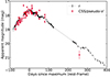 |
Fig. A.1. The light curve from the Catalina Sky Survey in pseudo-V band together with the r-band light curve of SN 2018ibb. |
Log of photometric observations
A.2. Large observing campaigns
2.2 m MPG — Between 16 December 2018 and 29 October 2019 (tmax+11 – tmax+283 days), we monitored the light-curve evolution with the seven-channel imager GROND (Gamma-Ray Burst Optical/Near-Infrared Detector; Greiner et al. 2008) from 4500 to 22,000 Å at the 2.2 m Max Planck Gesellschaft telescope at La Silla Observatory (Chile) as a part of the GREAT survey (Chen et al. 2018).
The images were reduced with the GROND pipeline (Krühler et al. 2008), which applies bias and flat-field corrections, stacks images and provides astrometric calibration. The photometry was extracted similarly to the ZTF data. To establish the absolute flux scale, we used a local sequence of stars from a cross-matched PanSTARRS-Gaia catalogue (griz) and 2MASS (JHK; Skrutskie et al. 2006). SN 2018ibb evaded detection in Ks band. These images are very shallow, and we omit them in this paper.
3.58 m ESO/NTT — At the end of October 2019, we switched from the 2.2 m MPG/ESO telescope to the 3.58 m ESO New Technology Telescope at La Silla Observatory (Chile). We obtained photometry in BVgriz between 22 October 2019 and 11 November 2020 (tmax+277 – tmax+619 days) with the EFOSC2 instrument (ESO Faint Object Spectrograph and Camera version 2; Buzzoni et al. 1984). Furthermore, we obtained a few epochs of JHK photometry with the SOFI (Moorwood et al. 1998). All observations were carried out as a part of the ePESSTO survey (Smartt et al. 2015). On 1 March 2022 (tmax+1023 days), we obtained a final image in B band. At this phase, the brightness of SN 2018ibb was well below the host level in the B band. We use these data to expand the host galaxy observations to shorter wavelengths.
The data were reduced with the PESSTO pipeline37 (Smartt et al. 2015), which applies bias and flat-field corrections, and provides astrometry calibration. We utilised the tool from Schulze et al. (2018) to extract the photometry. For the SN photometry, we used circular apertures and an elliptical aperture for the host galaxy whose size was matched to that of the VLT/FORS2 data. The BVgriz photometry was calibrated with a local sequence of stars from a cross-matched PanSTARRS-Gaia catalogue and the JHK photometry with the stars from the 2MASS point source catalogue.
8.2 m ESO/VLT — Between September 2020 and March 2021, we obtained photometry in gRIz with the FOcal Reducer/low dispersion Spectrograph 2 (FORS2, Appenzeller et al. 1998) at the 8.2 m Very Large Telescope at Paranal Observatory (Chile), covering the time interval from tmax+564 days to tmax+706 days. These data suffered from a progressively increasing contamination by the host galaxy. To remove the host contribution, we obtained a final set of gRIz photometry in January/February 2022 (tmax+991 days). These reference images were obtained under similar observing conditions, but their integration time was a factor of 2 larger to ensure a reliable host subtraction.
We reduced the data with IRAF in the same way as the GROND and NTT data. The world coordinate system was calibrated with the software package ASTROMETRY.NET (Lang et al. 2010). To remove the host contribution, we aligned all images in a given filter to the corresponding template image and subtracted the images with the HIGH ORDER TRANSFORM OF PSF AND TEMPLATE SUBTRACTION code version 5.11 (HOTPANTS; Becker 2015). We measured the brightness in the difference images using aperture photometry. The photometry was calibrated against a set of stars identified in archival griz CTIO/DECam images from the Dark Energy Survey (Dark Energy Survey Collaboration 2016) and DESI Legacy Imaging Surveys Dey et al. (2019)
Neil Gehrels Swift Observatory — We observed the field with the 30 cm Ultraviolet/Optical Telescope (UVOT; Roming et al. 2005) aboard the Swift satellite (Gehrels et al. 2004) between tmax+8.4 and tmax+224 days in w2, m2, w1, u, b, v. While SN 2018ibb was not observable from the ground between April and August 2019, we made strategic use of Swift’s orbit to reduce the seasonal gap of our ground-based campaigns from 100 to 54 rest-frame days.
We retrieved the science-ready data from the Swift archive38. We co-added all sky exposures for a given epoch and filter to boost the S/N using UVOTIMSUM in HEASOFT39 version 6.26.1. Afterwards, we measured the brightness of SN 2018ibb with the Swift tool UVOTSOURCE. The source aperture had a radius of 5″ while the background region had a significantly larger radius. The photometry was calibrated with the latest calibration files from September 2020.
A.3. Supplementary observations
We augmented the campaigns mentioned above with targeted observations using
-
the Alhambra Faint Object Spectrograph and Camera (ALFOSC)40 on the 2.56 m Nordic Optical Telescope (NOT) at the Observatorio del Roque de los Muchachos on La Palma (Spain) in griz
-
the 0.76 m Katzman Automatic Imaging Telescope (KAIT) in BVRI and ‘clear’ as part of the Lick Observatory Supernova Search (LOSS; Filippenko et al. 2001)
-
the Las Cumbres Observatory (LCO) in ugriz and BVRI
-
the optical imager (IO:O) on the robotic 2 m Liverpool Telescope (LT; Steele 2004) located at the Observatorio del Roque de los Muchachos in griz
-
the Low Resolution Imaging Spectrometer (LRIS, Oke et al. 1995) on the 10 m Keck I telescope at Maunakea (USA) in gVRi
-
the Multi-Object Double Spectrographs MODS-1 and 2 cameras in ugriz and the near-IR LUCI camera in JHK at the 8.4 m Large Binocular telescope at Mt. Graham (USA)
-
1 m Nickel telescope at Lick Observatory in BVRI (Li et al. 2003)
-
the SED Machine (Blagorodnova et al. 2018) at the Palomar 60-inch telescope at Mount Palomar (USA) in gri
-
the 28-inch telescope at the Wise Observatory (Israel) in gri
-
the Wide Field Camera 3 in F336W aboard the Hubble Space Telescope to obtain a late-time image in August 2022
All data were reduced in a similar fashion with instrument-specific pipelines, for example, FPIPE for the SEDm data (Fremling et al. 2016), the LOSSPHOTPYPELINE 41 for the KAIT and Lick data (Stahl et al. 2019) and IRAF. We applied aperture photometry to extract the photometry similar to the method described in Section A.2. In the case of KAIT and Lick data Point-spread function photometry (Stetson 1987) using DAOPHOT was applied.
The Keck observations were performed when the host contribution was non-negligible but smaller than 10% in all filters. Owing to the size of the host contribution, we omit any host correction but added an error of 0.2 mag in quadrature to those measurements. The NOT data were obtained in adverse observing conditions. We omit to report their photometry owing to issues in obtaining a reliable photometric calibration. The LCOGT z-band images suffer from fringing, resulting in photometry with large systematic errors. We omit to report these measurements in this paper.
Appendix B: Spectroscopic observations
B.1. 10 m Keck telescope
We obtained 3 epochs with LRIS between tmax−1.4 days and tmax+562.3 days. The first two observations, acquired on 1 December 2018 (tmax−1.42 days) and 29 August 2019 (tmax+231.2 days), used the B400/3400 blue-side grism and the R400/8500 red-side grating, the dichroic 560 and a 1 0 wide slit. The integration times were 300 s for each epoch. The third epoch was obtained with the B600/4000 blue-side grism and R400/8500 red-side grating and a 1
 0 wide slit on 18 September 2020 (tmax+562.3 days). The integration time was 4935 s. All spectra were reduced in a standard fashion with the data reduction pipeline LPIPE (Perley 2019).
B.2. Palomar 60-inch telescope
We acquired 3 epochs of spectroscopy with the SED Machine between tmax+5.4 and tmax+21.6 days. The SED Machine is a very low resolution (R ∼ 100) integral field unit covering the wavelength range from 3650 to 10 000 Å. The first two epochs (9 and 12 December 2018) are of sufficient quality and are reported to WISeREP but are not presented in the paper owing to the availability of higher resolution and higher S/N data. The final epoch obtained on 28 December 2018 is of very poor quality and is reported here only for completeness. All observations were reduced using the pipeline described by Rigault et al. (2019).
B.3. Palomar 200-inch telescope
We obtained one epoch of spectroscopy with the DouBle-SPectrograph (DBSP; Oke & Gunn 1982) on 13 December 2018 (tmax+8.8 days). The observations were taken using the D-55 dichroic beam splitter, a blue grating with 600 lines per mm blazed at 4000 Å, a red grating with 316 lines per mm blazed at 7500 Å, and a 1 5 wide slit. The data are reduced using the python package DBSP_DRP42 that is primarily based on PYPEIT (Prochaska et al. 2020a,b).
B.4. Extended Public ESO Spectroscopic Survey of Transient Objects
Between 15 December 2018 and 20 October 2019 (tmax+10.5 – tmax+275.6 days), we obtained 6 epochs of spectroscopy using EFOSC2. The observations were performed with grisms #11, #13 and #16. Depending on weather conditions, we used either a 1 0 or 1
 5 wide slit. The integration times were between 1800 and 5400 s. We reduced the data in a standard fashion using the PESSTO pipeline (Smartt et al. 2015).
B.5. 2.56 m Nordic Optical Telescope
We acquired 3 epochs of low-resolution spectroscopy with ALFOSC between 7 January and 22 February 2019 (tmax+30.8 and tmax+70.3 days). The spectra were obtained with a 1 3 wide slit and grism #4. For the second epoch, we used the second-order blocking filter WG345.
The data were reduced using IRAF (epoch 2), the pipeline FOSCGUI 43 (epochs 1 and 3). The reduction includes cosmic-ray rejection, bias corrections, flat fielding, and wavelength calibration using HeNe arc lamps imaged immediately after the target. The relative flux calibration was done with spectrophotometric standard stars observed during the same night.
B.6. 8.2 m ESO Very Large Telescope
X-shooter — We obtained 7 medium-resolution spectra with the X-shooter instrument (Vernet et al. 2011) between 10 January 2019 and 16 February 2020 (tmax+32.7 – tmax+377.5 days). All observations were performed in nodding mode and with 1 0/0
0/0 9/0
9/0 9 wide slits (UVB/VIS/NIR). The first four epochs covered the full spectral range from 3000 to 24,800 Å. For the other epochs, we used the K-band blocking filter (cutting the wavelength coverage at 20,700 Å; Vernet et al. 2011) to increase the signal-to-noise ratio (S/N) in the H band. The integration times were varied between 1800 and 3600 s.
The data were reduced following Selsing et al. (2019). In brief, we first removed cosmic-rays with the tool ASTROSCRAPPY
44, which is based on the cosmic-ray removal algorithm by van Dokkum (2001). Afterwards, the data were processed with the X-shooter pipeline v3.3.5 and the ESO workflow engine ESOReflex (Goldoni et al. 2006; Modigliani et al. 2010). The UVB and VIS-arm data were reduced in stare mode to boost the S/N. In the background limited case, this can increase the S/N by a factor of  compared to the standard nodding mode reduction. The individual rectified, wavelength- and flux-calibrated two-dimensional spectra files were co-added using tools developed by J. Selsing45. The NIR data were reduced in nodding mode to ensure a good sky-line subtraction. In the third step, we extracted the one-dimensional spectra of each arm in a statistically optimal way using tools by J. Selsing. Finally, the wavelength calibration of all spectra were corrected for barycentric motion. The spectra of the individual arms were stitched by averaging the overlap regions.
FORS2 — We obtained 3 low-resolution spectra with the FORS2 spectrograph between 20 September and 1 February 2022 (tmax+565.3 – tmax+989.2 days). Each observation was performed with the 300V grism and a 1 0 wide slit. The first epoch comprised of 6 × 1100 s (executed on 20 and 23 September), and the latter two epochs consisted of 12 × 1200 s each. The data were reduced with IRAF similar to the datasets mentioned above.
B.7. 3 m Shane telescope
We obtained a series of four spectra with the Kast double spectrograph46 mounted on the Shane 3 m telescope at Lick Observatory. These spectra span the time period tmax+24.3 through tmax+89.3 days. The Kast observations utilised the 2″ slit, 600/4310 grism, and 300/7500 grating. This instrument configuration has a combined wavelength range of ∼3500-10,500 Å. To minimise slit losses caused by atmospheric dispersion (Filippenko 1982), the Kast spectra were acquired with the slit oriented at or near the parallactic angle.
The Kast data were reduced following standard techniques for CCD processing and spectrum extraction (Silverman et al. 2012) utilising IRAF routines and custom PYTHON and IDL codes47. Low-order polynomial fits to comparison-lamp spectra were used to calibrate the wavelength scale, and small adjustments derived from night-sky lines in the target frames were applied. The spectra were flux calibrated using observations of appropriate spectrophotometric standard stars observed on the same night, at similar airmasses, and with an identical instrument configuration.
The spectrum from tmax+47.3 days was obtained in very poor conditions. The quality of the spectrum was insufficient to extract a useful spectrum.
B.8. 8.4 m Large Binocular Telescope
We observed SN 2018ibb in the optical with the Multi-Object Double Spectrographs MODS-1 and MODS-2 (Pogge et al. 2010) and in the near-IR with the two LUCI (LBT Utility Camera in the Infrared; Ageorges et al. 2010; Seifert et al. 2010) cameras. In the optical, we used MODS-1 and -2 in dual-grating mode (grisms G400L and G670L) providing a wavelength coverage from 3200–9500 Å and a slit mask with a width of  for each camera. The integration time was 0.8 hours for the observation on 22 October 2019 (tmax+276.1 days) and on 29/30 January 2020 (tmax+361.6 days). In the NIR, we used the G200 grating and a 1
 0 wide slit. The first epoch was obtained with the zJspec bandpass filter (0.90–1.25 μm) on 19 October 2019 (integration time 0.8 hours). A second epoch was obtained on 28 January 2020 in zJspec and HKspec (1.47–2.35 μm). The integration of each setup was 1 hour.
The MODS data were reduced first with MODSCCDRED (Pogge 2019) version 2.04 to remove the bias and flat-field the data using a slit-less pixel flat. After that, we used custom IRAF scripts to extract the science spectrum using a nearby star for tracing. The observations of the spectrophotometric standard were combined in order to measure the trace of the dispersion along the entire slit. This trace was used along with the wavelength calibration from arc-lamp lines to rectify the tilt in the direction of the dispersion and the cross-dispersion axes for the full-frame (8192 × 3072 pixel). The final wavelength calibration was cross-checked with known strong auroral skylines in the blue ([O I] λ 5577.338) and red ([O I] λ 6300.3) channels. The one-dimensional spectrum was extracted from each channel using a  -wide aperture. The spectra were flux-calibrated using the spectrophotometric standard stars. Telluric features were removed from the red channels using the normalised spectrophotometric standard spectrum. The data from the four channels were combined into a single spectrum and re-binned to a common scale of Δλ = 0.85 Å pixel−1. All data were corrected for heliocentric motion.
The LUCI spectroscopic data were reduced at the Italian LBT Spectroscopic Reduction Center48 by means of scripts optimised for LBT data adopting the standard procedure for long-slit spectroscopy with bias subtraction, flat-fielding, bad-pixel correction, sky subtraction, and cosmic-rays rejection. The wavelength calibration was obtained from sky-lines achieving an r.m.s. of < 0.3 Å in zJ and 0.9 Å in HK. We flux-calibrated the spectra with telluric standard stars.
B.9. 8.1 m Gemini-South telescope
We obtained one epoch of spectroscopy with the Gemini Multi-Object Spectrograph (GMOS; Hook et al. 2004; Gimeno et al. 2016) at the Gemini-South telescope at Cerro Pachon, Chile, starting on 28 January 2022 (tmax+988.1 days). We used the R150 grating with the GG455 blocking filter and a 1″-wide slit. We divided the observation into three sets of 4 × 1200 s each. Owing to technical problems, the campaign had to be aborted after the first set was obtained.
We reduced the data using the GEMINI IRAF package49 version 1.14. We detect the very faint trace of the SN 2018ibb, but due to the significantly shorter total integration time, the quality of the spectrum was insufficient to detect features of SN 2018ibb or its host galaxy.
Appendix C: Bolometric light curve
The tabulated version of the bolometric light curve is shown in Table C.1.
Bolometric luminosity and blackbody properties
Appendix D: VLT/FORS2 spectrum from January 2022
Figure D.1 shows the observed VLT/FORS2 spectrum from January 2022, the unbinned spectrum light-blue and a binned version in a darker shade (bin size 30 Å). We scaled the best fit of the host galaxy SED to the brightness at the SN explosion site (shown in red, galaxy emission lines are clipped). The shape of the continuum of the VLT spectrum is consistent with the host galaxy SED. The only remaining SN feature is the broad [O III] at 5000 Å.
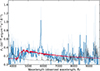 |
Fig. D.1. Observed spectrum of SN 2018ibb at tmax+989.2 days (unbinned: light blue, 30 Å binning: blue; error spectrum: grey) and the scaled galaxy SED (red). The only remaining SN feature is the broad [O III] λλ 4949,5007 emission line. |
Appendix E: Modelling the SN light curve with REDBACK
Table E.1 summarises the results of fitting the multi-band light curve with the software package REDBACK.
Light-curve fits with Redback: models, parameters, priors and marginalised posteriors
Appendix F: Galaxy photometry of SN 2015bn
We use science-ready coadded images from PanSTARRS DR1 and archival science-ready images obtained with MegaCAM at the 3.58 m Canada-France-Hawaii Telescope (CFHT). We augmente this data set with archival data from Swift/UVOT in w2, m2 and w1 obtained between January 2016 and February 2017 after the SN faded, and Subaru/Suprime-Cam (Miyazaki et al. 2002) in B and V bands.
The Swift/UVOT data is processed and analysed as described in Appendix A. The Subaru data is reduced with the software package SDFRED2 (Ouchi et al. 2004).
Photometry of SN2015bn’s host galaxy
The photometry is extracted using sufficiently large apertures to encompass the entire host galaxy. The instrumental magnitudes of the ground-based images is calibrated against stars from PanSTARRS. We apply known colour equations between PS1, SDSS and Bessell-like filters to account for differences in the filter response function as described in Section 3.1. A summary of the host photometry is reported in Table F.1.
We model the host SED with PROSPECTOR as described in Section 4.6. The observed SED is adequately described by a galaxy model with the stellar mass of  and a star-formation rate of
  (Figure F.1). We use the best-fit SED to remove the host contribution of the SN spectrum from Nicholl et al. (2018) in Section 5.4.
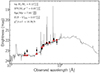 |
Fig. F.1. Spectral energy distribution (SED) of the host galaxy of SN 2015bn (black data points). The solid line displays the best-fitting model of the SED. The red squares represent the model-predicted magnitudes. The fitting parameters are shown in the upper-left corner. The abbreviation ‘n.o.f.’ stands for the number of filters. |
All Tables
Light-curve fits with MOSF IT: models, parameters, priors and marginalised posteriors.
Light-curve fits with Redback: models, parameters, priors and marginalised posteriors
All Figures
|
Fig. 1. False-colour image of the field when SN 2018ibb was bright (left) and after it had faded below the host level (right). The SN position, marked by the crosshair, is located ∼1 kpc from the centre of its star-forming dwarf host galaxy ( |
| In the text | |
|
Fig. 2. Galaxy absorption and emission lines at a common redshift of z = 0.166 in the supernova spectra at tmax+32.7 days (top) and at tmax+565.3 days (bottom). The error spectrum of each epoch is shown in grey. |
| In the text | |
|
Fig. 3. Multi-band light curve of SN 2018ibb from 1800 to 18 500 Å (rest-frame) after correcting for the Galactic extinction. SN 2018ibb was first detected by Gaia. The last non-detections before the first detection by Gaia and ATLAS are shown by the downward-pointing triangles. With a rise time of > 93 rest-frame days, SN 2018ibb is one of the slowest evolving SLSN known. The decline of 1.1 mag (100 days)−1 is similar to the decay time of radioactive 56Co. After tmax+575 days, the decline steepened to 1.5 mag (100 days)−1. The light curve shows undulations up to tmax+100 days and a longer-lasting bump at ∼300 rest-frame days. Vertical bars represent the epochs of spectroscopy and imaging polarimetry. The absolute magnitude is computed with M = m − DM(z)+2.5 log(1+z), where DM is the distance modulus and z the redshift. |
| In the text | |
|
Fig. 4. g-band light curve of SN 2018ibb in the context of the homogeneous ZTF-I SLSN sample. SN 2018ibb has a typical peak absolute magnitude. The rise of > 93 rest-frame days is significantly longer than of the average ZTF SLSN. The long-lasting rise implies a long diffusion time, which requires a very high total ejected mass. The high peak luminosity requires a very energetic explosion. Both properties together hint to an explosion mechanism that might be different from that of regular SLSNe. |
| In the text | |
|
Fig. 5. Bolometric light curve of SN 2018ibb from 1800 to 14 300 Å (rest-frame). The dotted lines indicate time segments with partial wavelength coverage. At peak SN 2018ibb reached a luminosity of > 2 × 1044 erg s−1. Integrating over the light curve from tmax–93 to tmax+706 days yields a radiated energy of 3 > ×1051 erg. Both values are conservative lower limits. The inset shows the evolution of the blackbody temperature and radius of the photospheric phase where photometry has been carried out from the u to H bands. The shaded regions indicate the 1σ statistical uncertainties. |
| In the text | |
|
Fig. 6. Spectroscopic sequence from 2500 Å to 10 000 Å and from the time of maximum to tmax+1000 days (rebinned to 5 Å and smoothed with a Savitzky–Golay filter). Spectra up to tmax+100 days (left panel) are characterised by a blackbody continuum with superimposed absorption lines from the SN ejecta, expanding with a velocity of ∼8500 km s−1. Between tmax+100 and tmax+225 days (while SN 2018ibb was behind the sun), the spectroscopic behaviour of SN 2018ibb evolved drastically. The late-time spectra (right panel) are characterised in the blue (< 5000 Å) by a pseudo-continuum and emission lines produced by the interaction of the SN ejecta with circumstellar material and in the red (> 5000 Å) by nebular emission lines from the 56Ni-heated SN core. The regions with the fastest evolution are highlighted by the grey-shaded regions. Figure 7 shows the identification of the most prominent features of the photospheric and nebular phases. Regions affected by strong telluric absorption were clipped. Their locations are indicated in Fig. 7. |
| In the text | |
|
Fig. 7. Line identification of the photospheric-phase spectrum (top) and nebular-phase spectrum (bottom). Top: The photospheric phase spectrum was fitted with the parameterised spectral synthesis code SYNOW (red curve). Most of the spectral features can be attributed to O I, Mg II, Si II, Ca II, and Fe II as seen in other SLSNe during their cool photospheric phase (Gal-Yam 2019a). In addition to the absorption lines in the SN ejecta, the photospheric phase spectrum shows conspicuous [Ca II] λλ 7291,7324, a feature that gets dominated by [O II] λλ 7320,7330 at about tmax+30 days. Bottom: The spectrum of the nebular phase consists of a blue pseudo-continuum and a series of allowed and forbidden emission lines from singly and doubly ionised oxygen, calcium, magnesium and iron. Remarkable is the presence of [O II] and [O III] in emission (as early as tmax+30 days), indicating ionising radiation from shock interactions (Sect. 5.1). SN absorption lines are indicated by dashed lines, and the locations mark the absorption trough minima (blueshifted by 8500 km s−1 from their rest wavelengths). SN emission lines are indicated by solid lines; their line centres are at the velocity coordinate v = 0. Regions of strong atmospheric absorption are grey-shaded. |
| In the text | |
|
Fig. 8. Spectroscopic sequence from 9500 to 21 500 Å. The spectral sequence covers the evolution of the photospheric (top) and nebular (bottom) phases. The NIR spectra at > 1 μm show only a few features in contrast to the optical spectra (Fig. 6). The most prominent features are labelled. All spectra were rebinned to 5 Å and smoothed with a Savitzky–Golay filter, except the spectrum at tmax+361.6 days that was rebinned to 10 Å. The grey scale at the bottom of each panel displays the strength of telluric features (white = transparent, black = opaque). In addition, regions of strong atmospheric absorption are grey-shaded. |
| In the text | |
|
Fig. 9. Zoom-in onto the Fe II absorption lines from the SN ejecta at selected epochs of the photospheric phase. The SN photosphere expands with a velocity of merely ≈8500 km s−1. There are no signs of deceleration between tmax and tmax+100 days. Starting at about tmax+30 days, emission from [O III] λλ 4959,5007 (grey shaded region), produced by the interaction of the SN ejecta with circumstellar material, contaminates the blue wing of Fe IIλ 5169. |
| In the text | |
|
Fig. 10. Maximum ejecta velocity. The extent of the Ca IIλ 3934 (black) absorption on the blue side can be traced to ∼ 12 500 km s−1 at tmax+32.7 days. Mg IIλ 2796 (dark grey) has a comparable maximum velocity, albeit this region is affected by additional SN features. The location of the blue and red doublet components of Mg IIλλ 2796,2803 and Ca IIλλ 3934,3968 of the host galaxy ISM are indicated by brackets in a darker shade at the top of the figure. We also mark the position of the doublets of the CSM shell with brackets in a lighter shade. The CSM shell is detected through an additional Mg II absorption-line system blueshifted by 2918 km s−1. The CSM shell is not detected in Ca II. |
| In the text | |
|
Fig. 11. Fe II ejecta velocities of SN 2018ibb and general SLSN samples (grey) at the time of maximum (top panel) and as a function of time (bottom panel). SN 2018ibb has a remarkably low velocity at the time of maximum and an unprecedentedly flat velocity evolution, which is in stark contrast to known SLSNe. |
| In the text | |
|
Fig. 12. Normalised X-shooter spectra from tmax+32.7 days to tmax+94.3 days (top panels) and their inverse-variance weighted co-added spectrum (bottom panel). The individual and stacked spectra show barely resolved, narrow absorption lines from the host ISM (marked by the solid vertical lines). In addition, a blue-shifted (2918 km s−1) absorption line system is visible (marked by the dashed vertical lines). The FWHMs of the blue-shifted component are 406 km s−1, significantly larger than the ISM lines but significantly smaller than the SN lines. This blue-shifted absorption-line system is connected with a shell of circumstellar material expelled by the progenitor star shortly before the explosion. No significant evolution in the position or shape of the absorption lines can be seen in the individual spectra (upper panels). The error spectrum is shown in grey. |
| In the text | |
|
Fig. 13. Impact of the light curve bump between tmax+240 and tmax+340 days on the SN spectrum at tmax+286.7 days. Top: The spectra before, during and after the light curve bump. Bottom: The observed spectrum at tmax+286.7 days (≈13 days before the peak of the bump) is shown in black. We estimate the “bump-free” spectrum of SN 2018ibb at tmax+286.7 days (red) based on the spectra obtained before and after the bump. The difference between the observed (black) and interpolated (red) spectra at tmax+286.7 days is shown in blue. It reveals a series of emission lines that can be attributed to [O II] and [O III]. An excess bluewards of 5000 Å is also visible, while no apparent residual can be seen at the location of [O I]. |
| In the text | |
|
Fig. 14. Thermal and non-thermal emission of SN 2018ibb. Less than a few percent of the total radiated energy is emitted in the radio and X-rays. The luminosity limits lie in the ballpark of non-detections of other SLSNe, and they are a factor of 50 larger than the luminosity of the four H-poor SLSNe with either radio or X-ray detection. The limits of SN 2018ibb are larger than the most luminous radio and X-ray SNe. |
| In the text | |
|
Fig. 15. Spectral energy distribution of the host galaxy from 1000 to 60 000 Å (black dots). The solid line displays the best-fitting model of the SED. The red squares represent the model-predicted magnitudes. The fitting parameters are shown in the upper-left corner. The abbreviation “n.o.f.” stands for the number of filters. |
| In the text | |
|
Fig. 16. Star-formation rate and stellar mass of the host galaxy of SN 2018ibb in the context of SLSN-I host galaxies from the PTF survey (Schulze et al. 2021). The host galaxy of SN 2018ibb lies in the expected parameter space of SLSN host galaxies but in the lower half of the mass and SFR distributions (kernel density estimates of the observed distributions are shown at the top and to the right of the figure). Its specific star-formation rate (SFR/mass) is comparable to the typical star-forming galaxies (grey band) but lower than for an average SLSN host galaxy. |
| In the text | |
|
Fig. 17. [O I] λλ 6300,6364 and Mg I] λ 4571 lines at tmax+286.7 days. The Mg I] line is well fitted with a parabolic shape (dark blue), expected from an optically thick expanding shell (e.g. swept up CSM and unshocked SN ejecta), while the [O I] lines show a strong blue deficit because the line-forming region is still optically thick. The [O I] doublet is centred on the 6364 Å doublet component. |
| In the text | |
|
Fig. 18. Late-time evolution of the [O I] λλ 6300,6364 doublet. Note the strong evolution on the blue side, while the red side of the lines is evolving slower. This indicates a transition from optically thick to optically thin [O I] lines, implying that the scattering in the absorption part of the P Cygni profile is decreasing. Regions of strong atmospheric absorption are grey-shaded. |
| In the text | |
|
Fig. 19. [O I] λλ 6300,6364, [O II] λλ 7320,7330, and [O III] λλ 4959,5007 line profiles at tmax+565.0 days. The velocity scale is centred on the blue doublet component in the left panel and on the red component in the right panel. [O II] and [O III] only reach out to approximately the velocity of the CSM shell (vCSM), much less than the photospheric velocity (vFeII) and the maximum velocity of the ejecta (vmax). In contrast to that, the [O I] profile extends to ⊈ 12 500 km s−1. This points to [O II] and [O III] being produced close to the CSM shell whereas [O I] is produced in the SN ejecta. |
| In the text | |
|
Fig. 20. Comparison of the [O III] λλ 4959,5007 lines with the [O III]λ 4363 line. These lines are produced by the interaction of the SN ejecta with circumstellar material. Due to the occulation of the CSM by an optically thick SN ejecta, less of the “backside” of the CSM is seen. The velocities of the CSM shell (vCSM), the photospheric velocity (vFeII) and the maximum velocity of the ejecta (vmax) are indicated. |
| In the text | |
|
Fig. 21. Evolution of the [O II] λλ 7320,7330 + [Ca II] λλ 7291,7324 line complex. Left: Up to tmax+565.0 days, the line complex is dominated by [O II]. The red wing narrows due to an increasing occultation of the CSM shell by the optically thick expanding SN photosphere. Right: Between tmax+565.0 days and tmax+637.2 days, the line complex shifts to the blue, consistent with the [Ca II] line becoming more dominant. All profiles are centred on [O II] λ 7320. |
| In the text | |
|
Fig. 22. Comparison of the [O II] λλ 7320,7330 lines with the O Iλ 7773 and O Iλ 9263 recombination lines. The similar line profiles, extending to ≲ 5000 km s−1 indicates an origin in a highly processed CSM shell. |
| In the text | |
|
Fig. 23. The bolometric light curve of SN 2018ibb from 1800 to 14 300 Å (rest-frame) and light-curve fits to the fading light curve using the Katz et al. (2013) method. The entire fading light curve from up to 706 days after peak is fully consistent by being powered 24–35 M⊙ of 56Ni (dark red), suggesting that SN 2018ibb could be a pair-instability supernova. At about 300 days after peak (i.e. ≳400 days after the explosion), the γ-ray trapping decreases with time. The loss of trapping is indicated by the difference between the light-red (100% trapping) and dark-red (< 100% trapping) curves. |
| In the text | |
|
Fig. 24. Modelling of the light curves from the rest-frame UV to the NIR with MOSFiT. All models provide an adequate description of the data up to tmax+400 days, though with differences in the fit quality. At later times, the models diverge. The pure nickel model is the only model that captures the evolution after tmax+500 days and has physically meaningful parameters. The central engine models (magnetar and fallback) predict a flattening of the light curve due to a power-law-shaped heating rate in contrast to powering by 56Ni that has an exponential energy deposition rate. The magnetar+nickel model also captures the full evolution. However, the inferred model parameters would be either physically implausible or require an exotic star, which we deem not viable. We note that the Keck photometry at tmax+539 days and tmax+562 days is not corrected for host contamination owing to the lack of Keck reference images to perform image subtraction. The expected host contribution is ≈10%. |
| In the text | |
|
Fig. 25. Comparison of SN 2018ibb with the PISN models P250Ni25 and P250Ni34 from Kozyreva et al. (2017; left panel) and the He100, He125, and He130 from Heger & Woosley (2002; right panel). Templates with nickel masses of 34–44 M⊙ are required to describe the entire bolometric light curve from tmax–93 to tmax+706 days. Models with M(Ni)=25 M⊙ systematically underestimate the observed bolometric light curve, but they could still be viable if CSM interaction contributes significantly throughout the evolution. |
| In the text | |
|
Fig. 26. Late-time spectra of SN 2018ibb at 287 and 637 days after its maximum. Overlaid are the computed PISN spectra from Jerkstrand et al. (2016) scaled to these epochs. The shaded region indicates the uncertainty of the explosion time. The He130 model provides an adequate description of the emission redwards of 6000 Å at tmax+286.7 days, but a worse match for the second epoch. The observed spectra show a considerable excess at shorter wavelengths that is not expected from the model spectra. We argue that the blue excess is due to the interaction of the SN ejecta with circumstellar material, which is not included in existing PISN models. The He100 model matches the observation of neither epoch. The vertical bars at the top of each panel indicate the location of telluric features. |
| In the text | |
|
Fig. 27. Nebular spectrum of SN 2018ibb (black) at tmax+637.3 days and its decomposition into a CSM interaction (blue) and PISN component (red). This decomposition reveals that the shape of the spectrum in the blue is similar to the pseudo-continuum seen in interaction-powered SNe (Type Ia-CSM, Ibn, Icn and IIn). The emission lines in the blue arise either from CSM interaction or from material in the CSM shell excited by the SN light. The dotted vertical lines indicate the location of strong galaxy emission lines. |
| In the text | |
|
Fig. 28. Observed late-time bolometric light curve (solid blue lines) and the fraction of light that could be attributed to 56Ni after accounting for CSM interaction (dashed, red). The dotted green curves show the 56Ni light curve after adding the missing IR flux (up to 5 μm). The IR correction pushes the light curves back to the regime of PISN models that produce 25–44 M⊙ of 56Ni. Even in the case of a substantial contribution from CSM interaction, a total amount of 25–44 M⊙ of 56Ni appears to be essential to power SN 2018ibb. |
| In the text | |
|
Fig. 29. Zoom-in of the region from 9000 Å to 10 500 Å at tmax+377.5 days. Cobalt has its strongest feature at 1.025 μm. Its tentative detection translates to 56Ni mass of ≳30 M⊙, consistent with the light curve modelling. The second strongest cobalt feature is at 9340 Å. Its location is indicated by a fiducial Gaussian centred 9340 Å. Its integrated luminosity is expected to be between 50 and 100% of [Co II] λ 1.025 μm. The absence of [Co II]λ 9340 is not an argument against the discovery of [Co II] λ 1.025 μm (see Sect. 5.2.5 for details). Lines from other elements that could blend with the [Co II] lines are marked. Regions of strong atmospheric absorption are indicated by vertical bars at the top of the figure. |
| In the text | |
|
Fig. 30. Photospheric velocity evolution of SN 2018ibb (probed with Fe II) and the predicted evolution from different PISN models. The synthetic velocities of the P250Ni25|34 and He130 models are very similar to the observed velocities and velocity evolution. These are also the models that match the observed bolometric light curve well, in particular the He130 model. |
| In the text | |
|
Fig. 31. SN 2018ibb in the context of the phenomenological sub-class of slow-evolving SLSNe. Even among this rare sub-class of SLSNe, SN 2018ibb with its exceptionally broad light curve and high peak luminosity is an extreme object with unprecedented properties. |
| In the text | |
|
Fig. 32. The bolometric light curves of SN 2018ibb and historical slow-evolving SLSNe in the context of PISN models with nickel masses between 5 and 44 M⊙. SN 2018ibb is the only SLSN whose entire light curve from tmax–93 to tmax+706 days is consistent with PISN templates. The other SLSNe have either too fast declining light curves, light curve shapes inconsistent with PISN models, or their light curves are poorly sampled, hindering a comparison with PISN templates. The grey-shaded region indicates the 1σ uncertainty. |
| In the text | |
|
Fig. 33. Fe II ejecta velocities of slow-evolving SLSNe (in colour) and general SLSNe samples (grey) at the time of maximum (top panel) and as a function of time (bottom panel). SN 2018ibb has a markedly low velocity at the time of maximum and a flat velocity evolution, which is in stark contrast to the bulk of the SLSN population. Its velocity at peak is similar to the slow-evolving SLSNe PS1-14bj and SN 2007bi. However, both comparison objects lack spectra at earlier and later times. |
| In the text | |
|
Fig. 34. Comparison of the spectra of SN 2018ibb to those of other slow-evolving SLSNe between tmax+30 days and tmax+1000 days (darker colour: 5 Å binning; light shade: unbinned spectra). Photospheric phase (Panels A–B): Around tmax (Panel A), the spectra of PTF12dam and SN 2015bn are characterised by a hot continuum with superimposed O II absorption lines as seen in many SLSNe at a similar epoch. SN 2007bi, LSQ14an and SN 2018ibb have cooler photospheres, and their spectra exhibit absorption lines from Ca, Fe, Mg, O and Si (see Fig. 7 for their locations) but not O II. At around tmax+60 days (Panel B), all spectra appear similar, though differences exist. LSQ14an, PS1-14bj, and SN 2018ibb are the only SLSNe showing [O III] in emission. Furthermore, SN 2007bi, LSQ14an and SN 2018ibb exhibit strong [Ca II]+[O II] in emission. This feature is also present in PTF12dam and SN 2015bn but is less pronounced. Nebular phase (Panels C–E): Differences start to emerge during the early nebular phase and become stronger with time. SN 2018ibb, LSQ14an and PS1-14bj continue to show conspicuous [O III] in emission, in contrast to PTF12dam, SN 2007bi and SN 2015bn that have very strong [O I] and O I in emission. SNe 2015bn and 2018ibb are the only SLSNe with spectra at ∼tmax+1000 days (Panel E). SN 2018ibb continues to show intermediate-width [O III], whereas the spectrum of SN 2015bn exhibits [O I]. The elevated noise in the SN 2018ibb spectrum at tmax+989.2 days at λ > 6000 Å is due to residuals of the skyline subtraction. The dashed vertical lines indicate the expected locations of emission lines commonly seen from H II regions. |
| In the text | |
|
Fig. 35. Late-time NIR spectra of SN 2018ibb and the slow-evolving SLSNe LSQ14an and SN 2015bn. The strongest features are labelled. SN 2018ibb is the only SLSN that shows cobalt in emission, which has its strongest optical-NIR feature at 1.025 μm. Its luminosity translates to a nickel mass of ≳30 M⊙, consistent with the light curve modelling. All spectra are scaled so that O Iλ 7773 has the same amplitude in all objects. Regions of strong atmospheric absorption are cropped. |
| In the text | |
|
Fig. A.1. The light curve from the Catalina Sky Survey in pseudo-V band together with the r-band light curve of SN 2018ibb. |
| In the text | |
|
Fig. D.1. Observed spectrum of SN 2018ibb at tmax+989.2 days (unbinned: light blue, 30 Å binning: blue; error spectrum: grey) and the scaled galaxy SED (red). The only remaining SN feature is the broad [O III] λλ 4949,5007 emission line. |
| In the text | |
|
Fig. F.1. Spectral energy distribution (SED) of the host galaxy of SN 2015bn (black data points). The solid line displays the best-fitting model of the SED. The red squares represent the model-predicted magnitudes. The fitting parameters are shown in the upper-left corner. The abbreviation ‘n.o.f.’ stands for the number of filters. |
| In the text | |
Current usage metrics show cumulative count of Article Views (full-text article views including HTML views, PDF and ePub downloads, according to the available data) and Abstracts Views on Vision4Press platform.
Data correspond to usage on the plateform after 2015. The current usage metrics is available 48-96 hours after online publication and is updated daily on week days.
Initial download of the metrics may take a while.