| Issue |
A&A
Volume 694, February 2025
|
|
|---|---|---|
| Article Number | A292 | |
| Number of page(s) | 28 | |
| Section | Stellar structure and evolution | |
| DOI | https://doi.org/10.1051/0004-6361/202452357 | |
| Published online | 24 February 2025 | |
Eruptive mass loss less than a year before the explosion of superluminous supernovae
I. The cases of SN 2020xga and SN 2022xgc
1
The Oskar Klein Centre, Department of Astronomy, Stockholm University, Albanova University Center, 106 91 Stockholm, Sweden
2
Center for Interdisciplinary Exploration and Research in Astrophysics (CIERA), Northwestern University, 1800 Sherman Ave, Evanston, IL 60201, USA
3
Instituto de Astrofísica de Canarias, Vía Láctea, 38205 La Laguna, Tenerife, Spain
4
Universidad de La Laguna, Departamento de Astrofísica, 38206 La Laguna, Tenerife, Spain
5
The Oskar Klein Centre, Department of Physics, Stockholm University, Albanova University Center, SE-106 91 Stockholm, Sweden
6
Nordita, Stockholm University and KTH Royal Institute of Technology, Hannes Alfvéns väg 12, 106 91 Stockholm, Sweden
7
Konkoly Observatory, Research Center for Astronomy and Earth Sciences, MTA Centre of Excellence, Konkoly Th. M. út 15-17, H-1121 Budapest, Hungary
8
Department of Experimental Physics, Institute of Physics, University of Szeged, Dóm tér 9, Szeged 6720, Hungary
9
Astrophysics Research Institute, Liverpool John Moores University, Liverpool Science Park, 146 Brownlow Hill, Liverpool L3 5RF, UK
10
European Southern Observatory, Alonso de Córdova 3107, Casilla 19, Santiago, Chile
11
Millennium Institute of Astrophysics MAS, Nuncio Monsenor Sotero Sanz 100, Off. 104, Providencia, Santiago, Chile
12
Center for Astrophysics and Cosmology, University of Nova Gorica, Vipavska 11c, 5270 Ajdovščina, Slovenia
13
Graduate Institute of Astronomy, National Central University, 300 Jhongda Road, 32001 Jhongli, Taiwan
14
Caltech Optical Observatories, California Institute of Technology, Pasadena, CA 91125, USA
15
School of Physics, University College Dublin, L.M.I. Main Building, Beech Hill Road, Dublin 4 D04 P7W1, Ireland
16
Division of Physics, Mathematics and Astronomy, California Institute of Technology, Pasadena, CA 91125, USA
17
Institute of Space Sciences (ICE, CSIC), Campus UAB, Carrer de Can Magrans, s/n, E-08193 Barcelona, Spain
18
Institut d’Estudis Espacials de Catalunya (IEEC), 08860 Castelldefels, (Barcelona), Spain
19
Department of Particle Physics and Astrophysics, Weizmann Institute of Science, 234 Herzl St, 76100 Rehovot, Israel
20
GRANTECAN, Cuesta de San José s/n, 38712 Breña Baja, La Palma, Spain
21
Las Cumbres Observatory, 6740 Cortona Dr. Suite 102, Goleta, CA 93117, USA
22
Department of Physics, University of California, Santa Barbara, CA 93106-9530, USA
23
Astronomical Observatory, University of Warsaw, Al. Ujazdowskie 4, 00-478 Warszawa, Poland
24
IPAC, California Institute of Technology, 1200 E. California Blvd, Pasadena, CA 91125, USA
25
Center for Astrophysics, Harvard & Smithsonian, 60 Garden Street, Cambridge, MA 02138-1516, USA
26
The NSF AI Institute for Artificial Intelligence and Fundamental Interactions, Massachusetts Institute of Technology, 77 Massachusetts Ave, Cambridge, MA 02139-4301, USA
27
Cardiff Hub for Astrophysics Research and Technology, School of Physics & Astronomy, Cardiff University, Queens Buildings, The Parade, Cardiff CF24 3AA, UK
28
LPNHE, CNRS/IN2P3, Sorbonne Université, Université Paris-Cité, Laboratoire de Physique Nucléaire et de Hautes Énergies, 75005 Paris, France
29
Department of Physics and Astronomy, University of Turku, 20014 Turku, Finland
30
Astrophysics Research Centre, School of Mathematics and Physics, Queens University Belfast, Belfast BT7 1NN, UK
31
Instituto de Alta Investigación, Universidad de Tarapacá, Casilla 7D, Arica, Chile
32
Dipartimento di Fisica “Ettore Pancini”, Università di Napoli Federico II, Via Cinthia 9, 80126 Naples, Italy
33
INAF – Osservatorio Astronomico di Capodimonte, Via Moiariello 16, I-80131 Naples, Italy
34
Department of Physics, University of Warwick, Gibbet Hill Road, Coventry CV4 7AL, UK
35
Astrophysics sub-Department, Department of Physics, University of Oxford, Keble Road, Oxford OX1 3RH, UK
⋆ Corresponding author; This email address is being protected from spambots. You need JavaScript enabled to view it.
Received:
24
September
2024
Accepted:
19
December
2024
Abstract
We present photometric and spectroscopic observations of SN 2020xga and SN 2022xgc, two hydrogen-poor superluminous supernovae (SLSNe-I) at z = 0.4296 and z = 0.3103, respectively, which show an additional set of broad Mg II absorption lines, blueshifted by a few thousands kilometer second−1 with respect to the host galaxy absorption system. Previous work interpreted this as due to resonance line scattering of the SLSN continuum by rapidly expanding circumstellar material (CSM) expelled shortly before the explosion. The peak rest-frame g-band magnitude of SN 2020xga is −22.30 ± 0.04 mag and of SN 2022xgc is −21.97 ± 0.05 mag, placing them among the brightest SLSNe-I. We used high-quality spectra from ultraviolet to near-infrared wavelengths to model the Mg II line profiles and infer the properties of the CSM shells. We find that the CSM shell of SN 2020xga resides at ∼1.3 × 1016 cm, moving with a maximum velocity of 4275 km s−1, and the shell of SN 2022xgc is located at ∼0.8 × 1016 cm, reaching up to 4400 km s−1. These shells were expelled ∼11 and ∼5 months before the explosions of SN 2020xga and SN 2022xgc, respectively, possibly as a result of luminous-blue-variable-like eruptions or pulsational pair instability (PPI) mass loss. We also analyzed optical photometric data and modeled the light curves, considering powering from the magnetar spin-down mechanism. The results support very energetic magnetars, approaching the mass-shedding limit, powering these SNe with ejecta masses of ∼7 − 9 M⊙. The ejecta masses inferred from the magnetar modeling are not consistent with the PPI scenario pointing toward stars > 50 M⊙ He-core; hence, alternative scenarios such as fallback accretion and CSM interaction are discussed. Modeling the spectral energy distribution of the host galaxy of SN 2020xga reveals a host mass of 107.8 M⊙, a star formation rate of 0.96−0.26+0.47 M⊙ yr−1, and a metallicity of ∼0.2 Z⊙.
Key words: supernovae: general / supernovae: individual: SN 2020xga / supernovae: individual: SN 2022xgc
© The Authors 2025
 Open Access article, published by EDP Sciences, under the terms of the Creative Commons Attribution License (https://creativecommons.org/licenses/by/4.0), which permits unrestricted use, distribution, and reproduction in any medium, provided the original work is properly cited.
This article is published in open access under the Subscribe to Open model. This email address is being protected from spambots. You need JavaScript enabled to view it. to support open access publication.
1. Introduction
Superluminous supernovae (SLSNe; Quimby et al. 2011; Gal-Yam 2012) constitute a rare class of massive star explosions (Perley et al. 2020) that reach absolute magnitudes between −20 and −23 mag at peak (De Cia et al. 2018; Lunnan et al. 2018a; Chen et al. 2023a). Today, more than 2001 SLSNe have been detected out to z = 2 (Angus et al. 2019). They are frequently found in low-metallicity dwarf host galaxies with high specific star formation rates (SFRs) (Neill et al. 2011; Chen et al. 2013, 2017; Lunnan et al. 2014; Leloudas et al. 2015; Angus et al. 2016; Perley et al. 2016; Schulze et al. 2018; Taggart & Perley 2021).
There are two types of SLSNe, which are differentiated by the presence or absence of hydrogen in their spectra (Gal-Yam 2012): hydrogen-poor (type I; SLSNe-I hereafter) and hydrogen-rich (type II; SLSNe-II hereafter). The early spectra of the majority of SLSNe-I could show a prominent blue continuum and a series of O II features at 3500 − 5000 Å, with the feature at 4350 − 4650 Å being the most dominant (Quimby et al. 2011, 2018; Mazzali et al. 2016). Studies (Mazzali et al. 2016; Dessart 2019; Könyves-Tóth 2022; Saito et al. 2024) have shown that the O II features require either nonthermal excitation and/or temperatures higher than 12 000–14 000 K; but in a few SLSNe-I (Nicholl et al. 2014; Gutiérrez et al. 2022; Schulze et al. 2024) this feature has not been detected in their spectra.
The high luminosities observed in SLSNe-I cannot be explained by the amount of radioactive 56Ni generated in the normal core-collapse process, which is the major power source of type I SNe, and thus alternative scenarios have been proposed. A popular scenario, which could potentially explain the majority of the observed properties in SLSNe-I (e.g., Inserra et al. 2013; Nicholl et al. 2017; Liu et al. 2017; Blanchard et al. 2020; Hsu et al. 2021; Chen et al. 2023b), is the spin-down of a newly formed rapidly rotating highly magnetized neutron star (NS) known as a magnetar (Ostriker & Gunn 1971; Kasen & Bildsten 2010; Woosley 2010; Vurm & Metzger 2021). Other proposed scenarios are the long-term fallback accretion of material onto a black hole (Dexter & Kasen 2013; Moriya et al. 2018), the thermonuclear explosion of 140 − 260 M⊙ zero-age main sequence (ZAMS) metal-poor stars referred to as pair-instability supernovae (PISNe; Barkat et al. 1967; Rakavy & Shaviv 1967; Woosley et al. 2002; Heger & Woosley 2002) and interaction of the SN ejecta with circumstellar material (CSM) formed by material previously expelled from the star (Chatzopoulos et al. 2012; Sorokina et al. 2016; Wheeler et al. 2017; Chen et al. 2023b).
The fate of the stars, their powering mechanism, and the type of the resulting explosion are closely related to the final years of their stellar lives before the core collapse. During their lifetime, stars can lose a substantial part of their initial mass due to stellar winds (e.g., Lucy & Solomon 1970; Lamers et al. 1999; Puls et al. 2008), binary interactions (e.g., Petrovic et al. 2005; Smith 2014; Götberg et al. 2017; Yoon et al. 2017; Petrović 2020; Laplace et al. 2020), or eruptive mass loss (e.g., Heger & Woosley 2002; Woosley et al. 2007; Quataert & Shiode 2012; Shiode & Quataert 2014; Smith & Arnett 2014; Smith 2014; Woosley 2017; Fuller & Ro 2018; Leung et al. 2019; Renzo et al. 2020; Leung et al. 2021). Mass loss in the form of violent outbursts becomes critical in the late stages of stellar evolution and, in extreme situations, can remove tens of solar masses. Such eruptive mass loss has been observed in η Carinae (Westphal & Neugebauer 1969) and is thought to come from a group of post-main-sequence stars called luminous blue variables (LBVs; Humphreys 1999).
Eruptive mass loss can also be achieved in the case of pulsational pair instability (PPI; Woosley et al. 2007; Woosley 2017; Leung et al. 2019) in which the formation of positron-electron pairs in the CO core of a star with mass as low as 40 M⊙ (if metallicity and rotationally induced mixing is taken into account; Chatzopoulos & Wheeler 2012a,b) ZAMS results in explosive O-burning, and the energy released drives a series of mass ejections. The more massive the star is, the more energetic the pulses are, and thus the more mass will be ejected in the pulses (Renzo et al. 2020). Woosley (2017) and Renzo et al. (2020) note that the time interval between the mass ejection and the core collapse in PPI could be between a few hours to 10 000 years, which, along with the ejection velocity, could determine the distance of the ejected material.
Eruptive mass loss, and especially PPI, can generate CSM shell(s) around the progenitor stars, which potentially can be seen in the spectra of the SNe. There are a few SLSNe-I in the literature with evidence of late-time mass loss, such as them showing late-time broad H emission (Yan et al. 2015, 2017a; Fiore et al. 2021; Pursiainen et al. 2022; Gkini et al. 2024) or early forbidden emission of [O II] and [O III] (Lunnan et al. 2016; Inserra et al. 2017; Aamer et al. 2024; Schulze et al. 2024) in their spectra. The former has been explained by interaction of the ejecta with H-rich CSM located at ∼1015 − 1016 cm (e.g., Yan et al. 2015), and the latter by the interaction with low-density matter moving at a few 103 km s−1. However, recently, two SLSNe-I, iPTF16eh (Lunnan et al. 2018b) and SN 2018ibb (Schulze et al. 2024), were discovered that show a unique spectroscopic feature, a second Mg II absorption system blueshifted by ∼3000 km s−1 with respect to the Mg II absorption lines originating in the interstellar medium of the host galaxy. This feature has been associated with the photoionization of a rapidly expanding CSM shell expelled decades before the explosion. In the case of iPTF16eh, Lunnan et al. (2018b) also detected a Mg II emission line that moved from −1600 km s−1 to 2900 km s−1 between 100 and 300 days after maximum light, and this was attributed to a light echo from that shell. The CSM was located at ∼1017 cm and matched with theoretical predictions of shell ejections due to PPI. However, the detections of these shells were both serendipitous, and so it is not known whether these properties are typical, or how common this phenomenon is.
We present results from a dedicated study using the X-shooter spectrograph (Vernet et al. 2011) on the ESO Very Large Telescope (VLT) in Paranal, Chile to search for a second Mg II absorption system. The full sample will be presented in a follow-up paper; here, we focus on the analysis of the two detections found in the X-shooter sample indicating the presence of a fast-moving CSM. An extensive dataset for SN 2020xga and SN 2022xgc enable us to extract the CSM shell properties and give insights into the late stages of the stellar evolution.
This paper is structured as follows. In Sect. 2, we present photometric and spectroscopic data for SN 2020xga and SN 2022xgc along with photometric measurements of their host galaxies, and imaging polarimetry data for SN 2022xgc. In Sect. 3, we analyze the light-curve properties of SN 2020xga and SN 2022xgc, derive their blackbody temperatures and radii, construct bolometric light curves, and compare them with a homogeneous sample of SLSNe-I as well as with the photometric properties of SN 2018ibb and iPTF16eh. We also model the light curves of SN 2020xga and SN 2022xgc under the assumption that they are powered by a magnetar. In Sect. 4, we present the spectroscopic sequences of SN 2020xga and SN 2022xgc, analyze the spectral properties of these two objects, and compare them with those of well-studied SLSNe-I, and with SN 2018ibb and iPTF16eh. The modeling of the Mg II lines to extract information about the CSM shell is done in Sect. 5. In Sect. 6, we discuss the properties of the two host galaxies. We discuss our findings and provide possible mass loss scenarios and alternative powering mechanisms in Sect. 7, and we summarize our results in Sect. 8.
Throughout the paper, the photometric measurements are reported in the AB system and the uncertainties are provided with 1σ confidence. We assume a flat Lambda cold dark matter cosmology with H0 = 67.4 km s−1 Mpc−1, Ωm = 0.31, and ΩΛ = 0.69 (Planck Collaboration VI 2020).
2. Observations
2.1. Our X-shooter sample
Motivated by the discovery of iPTF16eh and SN 2018ibb, we collected a sample of 19 SLSNe with the medium-resolution X-shooter spectrograph (program IDs: 105.20PN, 106.21L3, 108.2262 and 110.247C). The triggering criteria of the program were objects that have been already classified as SLSNe-I, were observable from Paranal and have z > 0.11 so that the Mg IIλλ2796, 2803 resonance lines are observable with X-shooter. Our primary objectives are to constrain the occurrence of such mass ejections in SLSNe-I and determine the distribution of the CSM properties. This paper focuses on the analysis of two detections in the X-shooter sample, SN 2020xga and SN 2022xgc, which exhibit a second narrow Mg II absorption system in their X-shooter spectra blueshifted by a few thousand km s−1 with respect to the Mg II absorption lines originating in the interstellar medium of the host galaxy.
2.2. Discovery and classification
2.2.1. SN 2020xga
SN 2020xga was discovered by the Panoramic Survey Telescope and Rapid Response System (Pan-STARRS1; Kaiser et al. 2010) as PS20jxm on the rise on October 4, 2020, at a w-band magnitude of 19.8 mag at right ascension, declination (J2000.0) 03h46m39.37s, −11° 14′33.90″ (Chambers et al. 2020). It was classified by the extended Public ESO Spectroscopic Survey for Transient Objects (ePESSTO+; Smartt et al. 2015) as a SLSN-I on November 6, 2020 (Gromadzki et al. 2020; Ihanec et al. 2020). An image of the field before and after the explosion is shown in Fig. 1a.
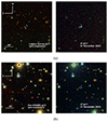 |
Fig. 1. Images of the fields of SN 2020xga (a) and SN 2022xgc (b). Panel a: Legacy Survey DR10 image of the field of SN 2020xga before explosion. A faint host galaxy at the SN position is visible, marked by the white crosshairs. Right: gri composite image of the SN near peak from Liverpool Telescope (LT). Panel b: Pan-STARRS image of the field of SN 2022xgc before explosion. The SN position is marked by the white crosshairs. Right: gri composite image of the SN near peak from the LT. All images have a size of 2 × 2 arcmin and have been combined following the algorithm in Lupton et al. (2004). |
Spectroscopic follow-up showed a redshift of z = 0.4296 (see Sect. 4.1) corresponding to a distance modulus of 41.93 mag. We corrected for the Milky Way (MW) extinction using the dust extinction model of Fitzpatrick (1999) based on RV = 3.1 and E(B − V) = 0.049 mag (Schlafly & Finkbeiner 2011). As for the host galaxy extinction, we find that the host properties of SN 2020xga are consistent with no extinction within the uncertainties (see Sect. 6). The estimated epoch of maximum light in the rest-frame g band is November 19, 2020, MJD = 59 172.5 (see Sect. 3.1).
2.2.2. SN 2022xgc
SN 2022xgc was discovered by the Zwicky Transient Facility (ZTF; Bellm et al. 2019; Graham et al. 2019; Dekany et al. 2020) on October 9, 2022, as ZTF22abkbmob at a g-band magnitude of 20.8 mag at right ascension, declination (J2000.0) 07h12m41.81s, +07° 18′59.95″ (Fremling 2022). ePESSTO+ classified it as a SLSN-I on December 2, 2022 (Gromadzki et al. 2022; Poidevin et al. 2022; Grzesiak et al. 2022).
To correct for the MW extinction, we again used the dust extinction model of Fitzpatrick (1999), RV = 3.1 and now with E(B − V) = 0.061 mag (Schlafly & Finkbeiner 2011). We adopted a spectroscopic redshift of z = 0.3103 (see Sect. 4.1) and computed the distance modulus to be 41.11 mag. Since the host of SN 2022xgc is not detected in the photometric catalogs, we did not apply any host extinction. The epoch of maximum light in the rest-frame g band is estimated to be November 18, 2022, MJD = 59 901.9 (see Sect. 3.1). An image of the field before and after the explosion is shown in Fig. 1b.
2.3. Photometry
Photometric measurements of SN 2020xga and SN 2022xgc are available from sky surveys such as the Asteroid Terrestrial-impact Last Alert System (ATLAS; Tonry et al. 2020), and the ZTF survey. We retrieved forced photometry from the ATLAS forced photometry server2 (Tonry et al. 2018; Smith et al. 2020; Shingles et al. 2021) for both c and o filters. The clipping and binning, with a bin size of 1 day, of the ATLAS data were done using the plot_atlas_fp.py3 python script (Young 2020). We removed the measurements with < 3σ significance and converted the resulting fluxes to the AB magnitude system using the 3631 Jy zeropoint. The ZTF forced point spread function (PSF)-fit photometry was requested from the Infrared Processing and Analysis Center (Masci et al. 2019) for the gri bands. To obtain the rest-frame light curve, we followed the ZTF data processing procedure4 including baseline correction, validation of the flux uncertainties, combining measurements obtained the same night and converting the differential fluxes to the AB magnitude system. Similarly to ATLAS data, a quality cut of 3σ was performed to the data.
In addition, both objects were monitored with the 2m Liverpool Telescope (LT; Steele et al. 2004) using the IO:O imager at the Roque de los Muchachos Observatory in the griz bands. The images were retrieved from the LT data archive5 and were processed through a PSF photometry script developed by Hinds and Taggart et al. (in prep.). Each measurement was calibrated using stars from the Pan-STARRS (Flewelling et al. 2020) catalog and a cut of 3σ was performed.
SN 2020xga was also monitored between November 2020 and July 2021 by ePESSTO+ using the Las Cumbres Observatory in the griz bands. We performed photometry using the AUTOmated Photometry of Transients6 pipeline developed by Brennan & Fraser (2022). The instrumental magnitude of the SN is measured through PSF fitting and the zero point in each image is calibrated with stars from the Pan-STARRS (Flewelling et al. 2020) catalog. We do not discuss the z-band photometry because of the poor quality of these images.
The photometric dataset of SN 2022xgc is complemented with four epochs obtained with the Rainbow Camera at the Spectral Energy Distribution Machine (SEDM; Blagorodnova et al. 2018; Rigault et al. 2019; Kim et al. 2022) at Palomar Observatory in the gri bands. The data were reduced with the FPipe pipeline described in Fremling et al. (2016). Finally, one epoch of photometry in the gr bands was obtained with the Alhambra Faint Object Spectrograph and Camera (ALFOSC) at the 2.56m Nordic Optical Telescope (NOT). For the reduction the PyNOT7 data processing pipeline was utilized. For nights with multiple exposures, we computed the weighted average and we kept only the data with > 3σ significance.
Overall, for SN 2020xga we obtained 68 epochs of photometry spanning from −44 and +59 days post maximum in the gcroiz bands with a cadence of 1.5 days in the best-covered r band. For SN 2022xgc we obtained 86 photometric epochs between −59 and +110 days after the peak in the gcroiz bands with an average cadence of 2 days in the g and r bands, which were best covered (for the photometric tables of SN 2020xga and SN 2022xgc see Sect. 8).
2.4. Spectroscopy
We acquired five low-resolution spectra of SN 2020xga between November 6, 2020, and December 30, 2020, and six low-resolution spectra of SN 2022xgc between December 1, 2022, and February 12, 2023, with the ESO Faint Object Spectrograph and Camera 2 (EFOSC2; Buzzoni et al. 1984) on the 3.58m ESO New Technology Telescope (NTT) at the La Silla Observatory in Chile under the ePESSTO+ program (Smartt et al. 2015). Additional medium-resolution spectra were obtained for both SN 2020xga between November 2020 and January 2021, and SN 2022xgc between December 2022 and March 2023, with the X-shooter spectrograph.
The spectroscopic data for SN 2022xgc was supplemented with three low-resolution spectra obtained with ALFOSC between November and December 2021, one spectrum obtained on November 22, 2022, with the Kast double spectrograph mounted on the Shane 3m telescope at Lick Observatory, and two spectra taken in November 2022 with the SEDM. We acquired one additional epoch of spectroscopy for SN 2020xga with the DouBle-SPectrograph (DBSP; Oke & Gunn 1982) mounted on Palomar 200-inch telescope on Palomar Observatory on January 07, 2021. Observations using the SEDM and DBSP were coordinated using the FRITZ data platform (van der Walt et al. 2019; Coughlin et al. 2023).
The NTT spectra were reduced with the PESSTO8 pipeline. The observations were performed with grisms #11, #13, and #16 using a  wide slit. The integration times varied between 1500 and 5400 s for SN 2020xga and between 900 and 4800 s for SN 2022xgc. The spectra of SN 2020xga on November 16 and 17, 2020, were combined to boost the signal-to-noise (S/N).
The X-shooter observations were performed for the ultra-violet (UV), visible (VIS), and near-infrared (NIR) arms in nodding mode using  ,
,  ,
,  wide slits, respectively, and were reduced using the ESO X-shooter pipeline. We followed the following procedure; first, the tool astroscrappy9 was used for the removal of cosmic-rays based on the algorithm of van Dokkum (2001), then the data were processed with the X-shooter pipeline v3.6.3 and the ESO workflow engine ESOReflex (Goldoni et al. 2006; Modigliani et al. 2010). The UV and VIS-arm data were reduced in stare mode. The corrected two-dimensional spectra were co-added utilizing tools developed by Selsing et al. (2019)10. To achieve proper skyline subtraction, the NIR-arm data were processed in nodding mode. The wavelength calibration of all spectra was adjusted to account for barycentric motion. The spectra of the separate arms were combined by averaging the overlap areas. Since observations of SLSNe-I have shown that the spectra tend to evolve slower compared to other SNe (e.g., Quimby et al. 2018), we stitched the X-shooter spectra of SN 2020xga on January 10 and 14, 2021, to increase the S/N.
The spectroscopic data obtained with ALFOSC were reduced using the PYPEIT11 pipeline (Prochaska et al. 2020a,b). The observations were obtained with a  wide slit and grism #4, and the exposure times were between 3344 s and 4000 s. The spectrum on November 13, 2022, was observed under cloudy conditions and thus we do not consider it. The SEDM observations had an integration time of 2250 s and were reduced using the pipeline described in Rigault et al. (2019). The first SEDM spectrum of SN 2022xgc obtained on November 14, 2022, is of insufficient quality and is not presented in the paper. The epoch observed with the DBSP instrument was taken using the D-55 dichroic beam splitter, a blue grating with 600 lines per mm blazed at 4000 Å, a red grating with 316 lines per mm blazed at 7500 Å, and a
  wide slit. The data were reduced using the python package DBSP_DRP412 that is primarily based on PYPEIT. Finally, the Kast observations utilized the
  wide slit, the 600/4310 grism, and the 300/7500 grating. The Kast data were reduced following standard techniques for CCD processing and spectrum extraction (Silverman et al. 2012) utilizing IRAF routines and custom Python and IDL codes13.
Each spectrum was flux calibrated against standard stars. The spectral logs for SN 2020xga and SN 2022xgc are presented in Tables B.1 and B.2, respectively.
2.5. Polarimetry
Linear polarimetry was obtained on SN 2022xgc at two epochs after maximum light at +26.1 (MJD 59928.0) days and at +60.1 (MJD 59962.0) days, observer-frame. A log of the observations is given in Table C.1. The polarimetry was obtained using a half wave plate in the FAPOL unit and a calcite plate mounted in the aperture wheel of the ALFOSC instrument on the NOT. The calcite plate provides the simultaneous measurement of the ordinary and the extraordinary components of two orthogonal polarized beams. The half wave plate can be rotated over 16 angle positions in steps of 22.5° from 0° to 337.5°. As a standard, we used 4 angle positions (0° ,22.5° ,45°, and 67.5°) to sample the linear Stokes Q − U parameters space.
The pipeline used to reduce the data is the same as the one introduced in Poidevin et al. (2022). The photometry of the ordinary and extraordinary beams was done using aperture photometry of size ∼2 to 3 times the Full-Width at Half-Maximum (FWHM) of punctual sources in the images. For multiple sequences of 4 Half-Wave Plate angles the polarization was obtained by summing-up the fluxes from the ordinary and extra-ordinary beams to minimize the propagation of the uncertainties. The instrumental polarization (IP) was first estimated using the unpolarized star HD 14069. The IP degree is of order 0.1% in the R-band, and or order 0.2% in the V-band (see Table C.2). These averaged Stokes  and
and  values were subsequently removed from the Stokes parameters Q − U estimates of the polarized calibration stars HD 251204 and BD+59 389 and of SN 2022xgc. The polarized stars were used to calculate the zero polarization angle (ZPA) used to rotate the Stokes Q, U parameters from the ALFOSC FAPOL instrument reference frame to the sky reference frame in equatorial coordinates. The polarization angles are counted positively from north to east. When applicable, the polarization degree and polarization angle obtained at each of these steps are reported in Table C.2.
2.6. Host galaxy observations
We retrieved science-ready co-added images from the DESI Legacy Imaging Surveys (LS; Dey et al. 2019) Data Release (DR) 10, and archival science-ready images obtained with MegaCAM at the 3.58 m Canada-France-Hawaii Telescope (CFHT) for SN 2020xga. We measured the brightness with the aperture photometry tool presented in Schulze et al. (2018) using an aperture similar to the other images. The photometry was calibrated against stars from the Sloan Digital Sky Survey DR9 (Ahn et al. 2012) and Pan-STARRS1 (Chambers et al. 2016). The host galaxy of SN 2022xgc is not detected in any catalog and thus, we provide the upper limits of the Dark Energy Survey images obtained with the Dark Energy Camera (DECam) at the Cerro Tololo Inter-American Observatory (CTIO). Table 1 summarizes the measurements in the different bands.
Photometry of the host galaxies of SN 2020xga and SN 2022xgc.
3. Photometry
3.1. General light-curve properties
To estimate the absolute magnitudes of SN 2020xga and SN 2022xgc, we used M = m − μ − AMW − Kcorr, where m is the apparent magnitude, μ is the distance modulus, AMW is the extinction caused by the MW, and the last term is the K-correction. For the last term, we used the expression −2.5log(1 + z), which we found to be consistent within 0.1 mag with the full K-correction using the spectra near peak, as is suggested in Chen et al. (2023a) as well. This gave Kcorr = −0.39 ± 0.1 mag for SN 2020xga and Kcorr = −0.29 ± 0.1 mag for SN 2022xgc. The multiband light curves in apparent and absolute magnitude systems for SN 2020xga and SN 2022xgc are shown in Fig. 2.
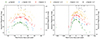 |
Fig. 2. Optical light curves of SN 2020xga (left panel) and SN 2022xgc (right panel). The magnitudes are corrected for MW extinction and K-correction. Upper limits are presented as downward-pointing triangles in a lighter shade. The epochs of the spectra are marked as thick lines at the top of the figure. The dashed line represents the estimated time of the first light. The x axis is in rest-frame days with respect to the rest-frame g-band maximum. |
To estimate the time of first light, we fit a baseline to the non-detection data points and a second-order polynomial to the rising part of the light curve, with the cross-point of the two fits being the time of first light. To estimate the uncertainty in the first-light epoch, we ran a Monte Carlo algorithm of randomly selected data points from a Gaussian distribution of the 1σ uncertainties for each of the selected flux measurements. For SN 2020xga, the resulting dates are MJD 59109.8 ± 0.2 in the g band and MJD 59110.5 ± 1.0 in the r band. We adopted a weighted average of MJD 59109.8 ± 0.2, which is also before the first c-band detection (MJD 59110.5). The uncertainty is statistical only, but the systematic error is likely a few days. This is shown for SN 2022xgc, where this method results in the dates of MJD 59836.5 ± 0.4 in the g band and MJD 59842.2 ± 2.6 in the r band. The weighted mean of MJD 59836.6 ± 2.5 is after the first three r-band detections, which could be associated with a pre-peak bump, as is seen in the light curves of some SLSNe-I (e.g., Leloudas et al. 2012; Nicholl et al. 2015b; Smith et al. 2016; Vreeswijk et al. 2017; Angus et al. 2019). These pre-bumps have been discussed in the context of shock breakout into a CSM (Piro 2015; Nicholl et al. 2015b; Smith et al. 2016; Vreeswijk et al. 2017) or a shock generated by a central magnetar at early times (Kasen 2017). Given that only three data points are shown in decline, we cannot conclusively favor one scenario over the other. However, since SN 2022xgc does not have stringent upper limits due to solar conjunction and the first r-band detections are real, we cannot exclude them and we instead took as time of the first light the first r-band data point MJD 59825.
To estimate the light-curve properties, we used the r-band light curve, which falls into the rest-frame g band at the redshifts of SN 2020xga and SN 2022xgc (Chen et al. 2023a). We used the method from Angus et al. (2019) for the light-curve interpolation and fit a Gaussian process (GP) regression, utilizing the PYTHON package GEORGE (Ambikasaran et al. 2015) with a Matern 3/2 kernel. We used the interpolated r-band light curve to estimate the peak magnitude as well as to define the rise and decline timescales as a fraction of the maximum flux (e.g., t1/2,rise is the time interval between fpeak/2 and fpeak) following Chen et al. (2023a). To estimate the rest-frame g − r color at the peak, we used the peak magnitudes inferred from the interpolated rest-frame g- and r-band light curves, K-corrected using the spectra closer to the peak. The photometric properties of SN 2020xga and SN 2022xgc obtained from this analysis are listed in Table 2. The timescales are reported in rest-frame days.
Light curve properties of SN 2020xga and SN 2022xgc.
In Fig. 3, we place the light curve properties of SN 2020xga and SN 2022xgc in the context of the homogeneous ZTF SLSN-I sample from Chen et al. (2023a), which studied the photometric properties of 78 H-poor SLSNe-I. In the four different panels, we show the kernel density estimates (KDEs) of the ZTF sample, which are an outcome of a Monte Carlo simulation accounting for the asymmetric errors. Both SN 2020xga and SN 2022xgc are placed in the bright side of the distribution while the decline times span across the whole distribution. The rise times and the g − r peak magnitudes are rather average compared to the median values of the ZTF sample.
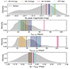 |
Fig. 3. Comparison of the photometric properties of SN 2020xga, SN 2022xgc, SN 2018ibb and iPTF16eh with the ZTF SLSN-I sample (Chen et al. 2023a). Top: KDE distribution of the Mg peak magnitudes for 78 ZTF SLSNe-I. Second: KDE plot of the e-folding rise time for 69 ZTF SLSNe-I. Third: e-folding decline time distribution for 54 ZTF SLSNe-I. Bottom: Rest-frame peak g − r color distribution for 39 ZTF SLSNe-I. The vertical colored lines along with the errors (shaded regions) illustrate the positions of SN 2020xga, SN 2022xgc, SN 2018ibb and iPTF16eh and the vertical black lines the median values of the ZTF sample. |
3.2. Bolometric light curve
To construct the bolometric light curves of SN 2020xga and SN 2022xgc, and derive the blackbody temperatures and radii, we constructed the spectral energy distributions (SEDs); however, we note that the presence of nonthermal sources affecting the SN spectra could introduce additional errors that are not accounted for in this analysis. We interpolated all light curves using the GP method described in Sect. 3.1 to match the epochs with r-band observations and converted the magnitudes to spectral luminosities Lλ for each band at each epoch. To extract information about the photospheric temperature and radius, we fit blackbody curves to each SED. The derived temperature and radius evolution for SN 2020xga and SN 2022xgc are plotted in Fig. 4. We compared only with events of the ZTF sample characterized as normal by Chen et al. (2023a). We find that the temperatures of both objects are comparable to those of the ZTF SLSNe-I and evolve similarly to the ZTF sample, declining over time. On the other hand, while the radius evolution of SN 2020xga and SN 2022xgc follows the rising trend seen for the SLSNe-I in the ZTF sample, the photospheric radius of both objects expands to larger values than for the rest of the ZTF sample. This is why these objects are so luminous while their temperatures are typical. In SN 2020xga and SN 2020xgc the photospheric radius decreases after 25 and 50 days, respectively. We caution that the quoted error bars are statistical only, and do not include any systematic effects; for example, from the fact that we are fitting to optical data only, while the peak of the blackbody is in the UV at early times (e.g., Arcavi 2022).
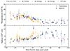 |
Fig. 4. Blackbody temperatures and radii of SN 2020xga, SN 2022xgc, SN 2018ibb and iPTF16eh. Top: Temperature evolution of SN 2020xga, SN 2022xgc, SN 2018ibb and iPTF16eh derived from the blackbody fits to the photometric (circle symbols) and the spectroscopic (star symbols) data. The gray background points represent the temperature evolution of the ZTF sample (Chen et al. 2023a). Bottom: Blackbody radius evolution of SN 2020xga, SN 2022xgc, SN 2018ibb and iPTF16eh utilizing photometry and spectra in comparison with the ZTF sample (gray). The arrows indicate the epochs where the X-shooter spectra of SN 2020xga and SN 2022xgc show the second Mg II absorption system. |
To construct the bolometric light curves of SN 2020xga and SN 2022xgc, we started by integrating the SED using only the gro filters, since the i and z light curves cover only a few epochs and the c filter is already covered by the g and r bands. To account for the missing flux in the NIR we fit a blackbody to the gro SED and integrated the blackbody tail up to 24 400 Å, beyond which the contribution to the bolometric light curve is negligible in the photospheric phase (∼1%; Ergon et al. 2013). For the UV correction, we followed the approach of Lyman et al. (2014) to capture the effect of the line blanketing commonly encountered in SLSNe (e.g., Yan et al. 2017b). To do this, we linearly extrapolated the SED from the observed g band to 2000 Å where the luminosity is set to zero. The total bolometric luminosity is the sum of the observed gro luminosity and the UV and NIR corrections. The bolometric light curves of SN 2020xga and SN 2022xgc are shown in Fig. 5. The peak bolometric luminosity is estimated to be Lbol, peak ≳ 2.7 ± 0.1 × 1044 erg s−1 for SN 2020xga and Lbol, peak ≳ 1.9 ± 0.1 × 1044 erg s−1 for SN 2022xgc. These values are typical for SLSNe-I being close to the median value of  erg s−1 reported for 76 SLSNe-I in Chen et al. (2023a) using the g and r filters and the value of
  erg s−1 found in Gomez et al. (2024) studying a heterogeneous sample of 262 SLSNe-I.
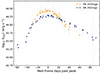 |
Fig. 5. Bolometric light curves of SN 2020xga and SN 2022xgc with bolometric corrections applied. The circles correspond to the derived luminosities using gro filters and the open square symbols illustrate the bolometric luminosity assuming the same bolometric correction as the nearest epochs with multiband data. The error bars represent statistical errors. |
To include the epochs for which we do not have complete gro data and for which we therefore cannot construct the SED, we assumed a constant bolometric correction. For SN 2020xga, for the later epochs that only have r-band data available, we used the same ratio of the r-band flux to the total flux that we measured at the latest epoch with multiband data. Similarly, for the rising part of the light curve for SN 2022xgc for which we have only g- and r-band measurements, we applied the same bolometric correction measured in the first multiband epoch. The bolometric luminosity used is the average of the luminosities calculated for the g and r bands. The data points assuming bolometric corrections are shown as open squares in Fig. 5. We note that this approach has two main caveats since at early phases the bolometric correction progressively underestimates the UV contribution while in the later phases the IR contribution gets more significant. By integrating the area below the bolometric light curves we estimated the total radiated energy to be Erad ≳ 1.8 ± 0.1 × 1051 erg for SN 2020xga and Erad ≳ 0.9 ± 0.2 × 1051 erg for SN 2022xgc. We note that these errors only account for the statistical errors in the fit and not for any systematic errors. These values are consistent within the uncertainties with the median  erg found in Gomez et al. (2024).
3.3. Photometric comparison to iPTF16eh and SN 2018ibb
In Fig. 3, we compare the light-curve properties of SN 2020xga and SN 2022xgc with the well-studied sample of SLSNe-I from the ZTF (Chen et al. 2023a). In this plot, we also include the photometric properties of SN 2018ibb (Schulze et al. 2024) and iPTF16eh (Lunnan et al. 2018b). These two SLSNe-I, at z = 0.166 and z = 0.427, respectively, are the only other SLSNe-I in which the two Mg II absorption-line system is detected in their spectra. To determine whether the objects with this remarkable spectroscopic similarity stand apart in photometry space, we also plot the rest-frame g-band peak magnitudes, rise and decline timescales, and g − r magnitudes at the peak of SN 2018ibb and iPTF16eh in Fig. 3. We note that since there are no data available in the rest-frame g band in the rising part of iPTF16eh’s light curve, we used the rest-frame u band to estimate the rise time.
Similarly to SN 2020xga and SN 2022xgc, SN 2018ibb and iPTF16eh are placed on the bright side of the ZTF luminosity distribution. The peak absolute magnitudes of these four objects span from −21.8 mag to −22.3 mag with a mean of −22.1 mag putting these objects among the most luminous SLSNe-I compared to the ZTF sample. The decline times of these four objects span across the whole distribution, while the g − r colors at the peak are close to the median value of the ZTF sample. The rise times of iPTF16eh, SN 2020xga and SN 2022xgc are consistent within the errors with the median of the sample, whereas SN 2018ibb is placed in the far slow end of the distribution as one of the longest rising SLSNe-I compared to the Chen et al. (2023a) sample.
The blackbody temperature and radius evolution of iPTF16eh and SN 2018ibb are plotted in Fig. 4. Both objects follow the temperature evolution of the ZTF sample, with iPTF16eh having higher temperatures compared to the bulk of the population. The photospheric radius of SN 2018ibb remains constant for almost 100 days after maximum light, while the radius evolution of iPTF16eh is increasing with time. However, similarly to SN 2020xga and SN 2022xgc, the size of the photoshere in iPTF16eh is getting larger than that of most ZTF SLSNe-I. The photospheric radius of iPTF16eh appears to decline after ∼60 days.
To better illustrate the variety in the photometric properties of these four objects, we plot the rest-frame g-band light curves in Fig. 6. The absolute magnitudes of all the objects are K-corrected and corrected for MW extinction. We see that the light curve of SN 2018ibb differs significantly compared to the other three SLSNe-I with a second Mg II system, by being very slow evolving and presenting bumps and undulations in its light curve. There are no signs of post-peak bumps or wiggles in the light curves of SN 2020xga, while the light curve of SN 2022xgc shows a possible flattening in the gcr bands starting ∼80 days after the peak (see Sect. 7). In SN 2022xgc, a pre-bump in the r band was observed immediately after explosion, whereas in SN 2020xga a possible bump can be seen in the g and r band light curves at ∼ − 30 days. All four objects are very energetic with radiated energies of Erad ≳ 1 × 1051 erg s−1.
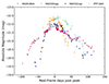 |
Fig. 6. Rest-frame g-band absolute magnitude light curves of SN 2020xga and SN 2022xgc in comparison with iPTF16eh and SN 2018ibb. The magnitudes are K-corrected and corrected for MW extinction. The x axis is in rest-frame days with respect to the g-band peak, with the exception of iPTF16eh, where the u band was utilized for estimating the peak owing to the lack of data in the rising part of the g-band light curve. |
3.4. Light-curve modeling
We modeled the observed multiband light curves of SN 2020xga and SN 2022xgc using the Bayesian inference software package for fitting electromagnetic transients, REDBACK (Sarin et al. 2024). We input the redshift of the SLSNe (see Sect. 4.1), the gcroi photometric observations of SN 2020xga and SN 2022xgc corrected for extinction (we excluded the z band due to the low number of datapoints), and a list of priors shown in Table 3. We explored the parameter space with the nested sampling package DYNESTY (Ashton et al. 2019; Speagle 2020).
Priors and posterior of the parameters fit with REDBACK for the generalized magnetar model.
To fit the data, we selected the versatile general magnetar-driven supernova model described in Omand & Sarin (2024) under the assumption that the light curves of SN 2020xga and SN 2022xgc are powered by the spin-down of a rapidly rotating newly formed magnetar (Ostriker & Gunn 1971; Arnett & Fu 1989; Kasen & Bildsten 2010; Chatzopoulos et al. 2012; Inserra et al. 2013). This model sets the magnetar braking index, n, as a variable, relaxing the assumption of a vacuum dipole spin-down mechanism and includes the dynamical evolution of the ejecta (Sarin et al. 2022) coupling it to both the explosion energy and the spin-down luminosity of the magnetar itself. We used the default priors defined in Omand & Sarin (2024) relaxing the priors for the explosion energy ESN and the temperature floor Tfloor. The opacity, κ, was fixed at 0.04 cm2 g−1, which is a good approximation for type Ic SNe, as is shown in Kleiser & Kasen (2014) (see their Fig. 3) considering that the blackbody temperature tends to overestimate the temperature of the photosphere (Dessart 2019). We note that if we set the κ parameter free, our results do not change significantly, suggesting that the choice of opacity plays a minimal role in our inference. However, we note that the opacity is kept constant with time and a time-dependent opacity could yield different results. This model assumes a modified SED accounting for the line blanketing in the UV part of the SLSN spectra (Chomiuk et al. 2011) similar to the one used in Nicholl et al. (2017). The REDBACK light curve fits are shown in Fig. 7, and the resulting values of the posteriors are given in Table 3. The corner plots are uploaded in https://zenodo.org/records/14565605 (see Sect. 8).
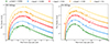 |
Fig. 7. Multiband light curves of SN 2020xga (left panel) and SN 2022xgc (right panel) with their resulting fits from REDBACK. The solid colored lines indicate the light curves from the model with the maximum likelihood, while the shaded areas depict the 90% credible interval. The x axis is in rest-frame days with respect to the rest-frame g-band maximum. |
In SN 2020xga (Fig. 7; left panel), the model captures well the rise (apart from the i band, which does not have data during the rise), peak, and decline in all five filters up to 30 days, after which the model declines more slowly than the data. The model fails to fit the first real detection in the c band and a possible small bump at ∼ − 30 days that is visible in the g and r bands. The latter is not unexpected since this model can explain only a smooth light curve (see discussion in Omand & Sarin 2024). Similarly, in SN 2022xgc (Fig. 7; right panel), the model fits well the SN multiband light curve both in the rise and the decline up to ∼60 days, after which the model declines more quickly than the data in the r and c bands. In addition, the model does not capture the first three data points in the r band, which, as is discussed in Sect. 3.1, could potentially be a pre-bump often seen in the light curves of SLSNe-I. A possible explanation for the early bumps could be interaction with extended material (Piro 2015) or magnetar-driven shock breakout (Kasen 2017).
The general magnetar-driven supernova model uses the initial magnetar spin-down luminosity, L0, and the magnetar spin-down time, tSD, as input parameters instead of the initial magnetar spin period in millisecond, P0,ms( = P/103 s), the magnetic field, B14(=B/1014 G), and the NS mass, MNS, used in previous magnetar models (e.g., Nicholl et al. 2017). To recover these parameters, we used the scalings
 (1)
(1)
and
 (2)
(2)
Assuming a 1.4 M⊙ NS with the same equation of state as in Nicholl et al. (2017), we found the rotational energy of the magnetar, Erot, to be 1.1 × 1052 erg for SN 2020xga and Erot = 3.3 × 1052 erg for SN 2022xgc, while P0,ms is estimated to be 1.6 ± 0.1 and 0.9 ± 0.2 for SN 2020xga and SN 2022xgc, respectively. The estimated P0,ms values in SN 2020xga and SN 2022xgc are close to the so-called mass-shedding limit, the limit at which the centrifugal force throws mass off the surface of the magnetar (e.g., Metzger et al. 2015; Watts et al. 2016).
The ejecta masses of 7.0 M⊙ and 9.3 M⊙ for SN 2020xga and SN 2022xgc, respectively, resulting from the general magnetar-driven supernova model, are consistent with the findings of Chen et al. (2023b), who found that the median ejecta mass is  . However, we note that this comparison is limited by the different physics included in the model used in this paper and the model of Nicholl et al. (2017) used in the paper of Chen et al. (2023b). In addition, the model estimates the explosion dates, texp, of SN 2020xga and SN 2022xgc to be 13 and 1 days, respectively, which are earlier than the values found in Sect. 3.1. These small discrepancies are not unreasonable given that both SNe were luminous already at the time of the first detection, and thus our approach in Sect. 3.1 constrains the time of first light rather than the explosion date.
Since the ejecta velocity, vej, in the general magnetar-driven supernova model is not constant and the ejecta evolve dynamically as a function of time, we calculated the diffusion timescale, tdiff,
 (3)
(3)
using the ejecta velocity at the peak. The vej at the peak derived from the most likely model in REDBACK is 10 446 km s−1 for SN 2020xga and 8304 km s−1 for SN 2022xgc, and thus the tdiff is estimated to be 18 days and 24 for SN 2020xga and SN 2022xgc, respectively. We note that the ejecta velocities calculated in REDBACK do not have the same physical meaning as the line velocities extracted from the spectra in Sect. 4.3. By computing the ratio of tSD/tdiff, we could determine the fraction of the spin-down luminosity converted to kinetic energy accelerating the ejecta (Suzuki & Maeda 2021; Sarin et al. 2022). The ratios of the two timescales are 7.6 for SN 2020xga and 6.6 for SN 2022xgc. These two ratios show that the radiated and kinetic energy could be possibly dominated by magnetar spin-down (Suzuki & Maeda 2021; Omand & Sarin 2024). We note that a discussion of alternative power-mechanism scenarios is included in Sect. 7.4.
3.5. Imaging polarimetry
The polarization degrees obtained on SN 2022xgc, and reported in Table C.2 are all very low (< 0.5%), and all constrained to about or less than 2σ. The final values shown in bold (Column 9) were obtained after bias correction following the equation given in Wang et al. (1997):
 (4)
(4)
where h is the Heaviside function, Pobs is the observed polarization, and σP is the 1σ error.
The debiased measurements obtained on SN 2022xgc displayed in the last column of Table C.2 have been obtained without making any MW polarization correction. The first important point to notice is that they all show that the percentage of polarization is consistently low and does not seem to vary with time. The second important point is that these measurements are all consistent with the low level of Galactic polarization expected in that region of the sky. The Galactic extinction along the line of sight at the coordinates of SN 2022xgc is such that E(B − V) = 0.061 (Schlafly & Finkbeiner 2011). Following Serkowski et al. (1975), this means that, in case of a magnetic field perfectly lying on the plane of the sky, the empirical upper limit on the optical degree of polarization produced by dichroic absorption by magnetically aligned Galactic dust grains should be Pmax = 9 × E(B − V) = 0.55%. A look at the measurements of the two closest known polarized stars in the vicinity of SN 2022xgc, HD 58784 with PV = 0.65 ± 0.2% and HD 57291 with PV = 0.37 ± 0.2%, support this statement. These data were retrieved from the compiled catalog of optical polarization measurements by Heiles (2000).
The polarization angles displayed in Table C.2 show polarization angles that differ by about 90° between the two epochs. The constraints on the polarization angles are low S/N, but as an ultimate test we estimated the variations in the polarization degree obtained between each epoch in each filter. This was done using the values of the Stokes parameters before debiasing the data. Any IP and ZPA corrected Stokes parameter on SN 2022xgc should be the sum of a constant contribution from the MW and from the host galaxy (if any) added to a possibly variable contribution from the SN. Therefore a differential measurement between two epochs should assess the degree of variation in polarization associated to the SN. In the R-band the differential is, ΔP(R) = 0.29 ± 0.16%, while in the V-band it is, ΔP(V) = 0.52 ± 0.23%.
We conclude that the estimates given in Table C.2 are likely estimates of the MW polarization contribution and that any contribution that could be associated with SN 2022xgc and its host galaxy should only be a few tenths of a percent. This low level rejects any detection of jet activities. If the level of polarization associated with SN 2022xgc changed between the two epochs, it should only be a fraction of a percent; in other words, very low. This low level of variation in the polarization level refutes the idea that there is any strong change in the shape of the photosphere of the SN between the two epochs.
All these results seem consistent with the statistical results obtained by Pursiainen et al. (2023) on a sample of 16 SLSNe. In this work, the data obtained before maximum light indicate nearly spherical photospheres. No clear relation is found between the polarimetry and spectral phase after maximum light, and an increasing polarization degree is measured only on a subsample of four SLSNe that have irregular light curve shapes on decline. The light curve decline of SN 2022xgc looks smooth and regular (see Fig. 7, right) at the phases when polarimetry was obtained (+26.1 days and +60.1 days). If any strong CSM interaction with the ejecta of SN 2022xgc happened during these two phases, it appears that it did not affect the symmetry of the system. We point out, however, that these results are not indicative of the lack of CSM playing a role in powering the observed light curve of the events.
4. Spectroscopy
4.1. Redshift
To estimate the precise redshifts of SN 2020xga and SN 2022xgc, we examined the X-shooter spectra of SN 2020xga at −8.3 days and SN 2022xgc at +21.9 days after maximum light and identified emission and absorption lines from the interstellar medium and H II regions in the host galaxy (e.g., Vreeswijk et al. 2014; Leloudas et al. 2015). Figure 8 shows the galaxy lines that appear in the spectra of SN 2020xga and SN 2022xgc and that we used for the redshift determination.
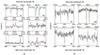 |
Fig. 8. Host galaxy absorption and emission lines in the X-shooter spectrum of SN 2020xga (panel a) −8.3 days and SN 2022xgc (panel b) +21.9 days after maximum light. The vertical lines illustrate the various redshift values of the galaxy lines. Panel a: In the spectrum of SN 2020xga,, the emission lines (dashed red lines) give a consistent redshift of z = 0.4287, whereas the strong (dashed blue line) and weak (dashed gold line) absorption lines indicate redshifts of z = 0.4283 and z = 0.4296, respectively. Panel b: The host galaxy lines (dashed gold line) of SN 2022xgc agree on a redshift of z = 0.3103. |
We identified in the spectrum of SN 2020xga the galaxy’s narrow absorption Fe II doublet λλ2586, 2600 and Mg II doublet λ2796, 2803, and the galaxy’s narrow emission [O II] doublet λλ3727, 3729, Hβλ4861, forbidden [O III] doublet λλ4959, 5007 and narrow Hαλ6563. We found two galactic Fe II and Mg II absorption systems in the spectrum of SN 2020xga, with the stronger lines at a redshift of z = 0.4283 ± 0.0002 and the weaker lines at z = 0.4296 ± 0.0002. In addition, the host’s emission lines are consistent with a redshift of z = 0.4287 ± 0.0001. Throughout the paper, we chose the redshift of SN 2020xga, as the higher value, and hence we assumed z = 0.4296. We further discuss this implication in Sect. 6.
In the case of SN 2022xgc, the host galaxy is not detected in the images since it falls below the sensitivity limits of the surveys (see Table 1); however, host galaxy lines are detected in the X-shooter spectrum of SN 2022xgc. This is not unprecedented since it has been also seen in other SLSNe-I (e.g., Vreeswijk et al. 2014; Chen et al. 2015; Leloudas et al. 2015). The host galaxy lines displayed in the spectrum of SN 2022gxc are the narrow Fe II doublet λλ2586, 2600, the Mg II doublet λλ2796, 2803, the Mg Iλ2852 and Hαλ6563. These lines support a redshift of z = 0.3103 ± 0.0001 for SN 2022xgc.
4.2. Spectroscopic sequence
Figure 9 depicts the spectral evolution from −9.0 to +37.8 rest-frame days past maximum brightness of SN 2020xga and from −0.7 to +92.1 rest-frame days of SN 2022xgc from 2500 Å up to ∼10 000 Å. All spectra were taken during the photospheric phase. As the ejecta cools down, the spectra of both SN 2020xga and SN 2022xgc begin to resemble those of typical type Ic SNe, which is expected for SLSNe-I (Gal-Yam 2019a).
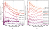 |
Fig. 9. Spectral sequence of SN 2020xga (panel a) from −9 to +37.8 rest-frame days and SN 2022xgc (panel b) from −0.7 to +92.1 g-band rest-frame days. An offset in flux was applied for illustration purposes. The spectroscopic measurements have undergone absolute flux calibration to align with the photometric data. The spectra are corrected for MW extinction and are smoothed using a Savitzky-Golay filter. The original data are presented in lighter colors. Regions of strong atmospheric absorption are blue-shaded. |
To identify the spectral lines in SN 2020xga and SN 2022xgc we used the medium-resolution X-shooter spectra due to their high S/N. For SN 2020xga, the spectra at −8.3 and +37.8 days were utilized, and for SN 2022xgc, we used those at +21.9 and +92.1 days. The line identification was done by comparing the spectra with well-studied SLSNe-I from the literature (e.g., Quimby et al. 2011, 2018; Inserra et al. 2013; Nicholl et al. 2015b; Gal-Yam 2019b), by modeling the earlier spectra at −8.3 days and +21.9 days (for SN 2020xga and SN 2022xgc, respectively) using the synthesis code SYN++ (Thomas et al. 2011) and finally by searching the National Institute of Standards and Technology (NIST; Kramida et al. 2022) atomic spectra database for lines above a certain strength, similar to what was done in Gal-Yam (2019b). Figure 10 depicts the X-shooter spectra of SN 2020xga and SN 2022xgc along with the most prominent features blueshifted by 6000–8000 km s−1 to match the absorption lines (see Sect. 4.3). The CaH [MYAMP] K and Mg I] lines in the spectra at +37.8 days and +92.1 days are shown at zero rest-frame velocity. The SYN++ modeling of the −8.3 day phase spectrum of SN 2020xga and the +21.9 day phase spectrum of SN 2022xgc can be found in Fig. D.1, while Table D.1 collects the best-fit parameter values obtained by the modeling.
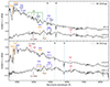 |
Fig. 10. X-shooter spectra of SN 2020xga (upper panel) at −8.3 and +37.8 days and SN 2022xgc (lower panel) at +21.9 and +92.1 days after maximum light. The spectra are corrected for MW extinction and are smoothed using a Savitzky-Golay filter. The original spectra are shown in lighter gray. The most conspicuous features are labeled. Uncertain line identifications are denoted with question marks. The ions beneath the spectrum are shown at the rest wavelength, whilst those above have been shifted to match the absorption component. The light blue regions represent the telluric absorptions. |
In the early spectrum of SN 2020xga, SYN++ tentatively identify the strong W-shape feature between 3500–5000 Å with the O IIλ4358 and λ4651 that characterize the spectra of numerous SLSNe-I. A small contribution of C II might be present at the troughs of 4300 and 4550 Å. Comparison with other SLSNe-I showed that the absorption trough at 4300 Å is most likely a blend of Fe IIIλ4432 and O IIλ4357. Redward of the O II lines, the Fe IIλ4923 and λ5169 are present, but the Fe IIλ4923 falls into the telluric band and the Fe IIλ5169 is likely mixed with Fe IIIλ5129 (Liu et al. 2017). Above 5000 Å the early spectrum of SN 2020xga does not show any obvious feature. Blueward of 3500 Å a number of features are visible, but owing to severe blending the identification is challenging. The trough at 2670 Å is associated with Mg II, as is seen in other SLSNe-I, and the trough at ∼2880 Å has been observed in a number of SLSNe (e.g., Vreeswijk et al. 2014; Quimby et al. 2018; Gkini et al. 2024) and has been suggested by a few studies (Dessart et al. 2012; Mazzali et al. 2016; Quimby et al. 2018; Gkini et al. 2024) to have some contribution from Ti III, Fe III, Si III, C II and Mg II. Searching NIST, we discovered that the absorption at 3200 Å could be attributed to Fe IIλ3325 and Fe IIIλ3305. The feature at 3410 Å may be related with Fe IIλ3500.
In the spectrum of SN 2022xgc at +21.9 days the major ions that are securely identified by SYN++ are Fe II, Si II and Ca II. Comparison with other SLSNe-I revealed that the absorption trough at 2670 Å is due to Mg II. The absorption component at 2880 Å is stronger than what is seen in SN 2020xga and similar to the one observed in the SLSN-I SN 2020zbf (Gkini et al. 2024). As was previously stated, this component is likely a contribution of multiple elements, including Mg II. Searching the NIST, we identified some plausible contribution of Fe II between 3000 and 3600 Å, although the high level of blending makes this identification dubious. Additional Mg IIλ4481 may be present in the absorption feature at 4300 Å. Absorption from O II between 3500–5000 Å, as is seen in many SLSN-I spectra around the peak, is not present. Similarly to the case of SN 2020xga, we were unable to identify any line beyond 6500 Å in the spectrum of SN 2022xgc owing to low S/N.
The spectra of SN 2020xga at +37.8 days and SN 2022xgc at +92.1 days resemble the spectra of a SN Ic at maximum light (Pastorello et al. 2010; Quimby et al. 2011). Both objects show Ca IIλλ3966, 3934 (though in SN 2020xga the emission line is weak), Mg IIλ4481, Mg I] λ4571, and strong Fe II lines between 4000 and 5200 Å blueshifted by 7500 km s−1 (see Sect. 4.3) to match the absorption component. In SN 2022xgc, the strong absorption trough at 6230 Å is connected with Si IIλ6355, whereas in SN 2020xga, Si II may contribute to the weak absorption component at 6230 Å. The contribution of the O I triplet λλ7772, 7774, 7775 in the spectra of SN 2020xga and SN 2022xgc might be visible at 7580 Å, however owing to the low S/N, this identification is uncertain.
4.3. Ejecta velocities
The ejecta velocities of SLSNe-I and their evolution can be measured from the O II absorption lines at 3500–5000 Å at early phases (Quimby et al. 2018; Gal-Yam 2019b,a) and from the Fe II triplet λλ4923, 5018, 5169 (Branch et al. 2002; Nicholl et al. 2015a; Modjaz et al. 2016; Liu et al. 2017). In SN 2020xga, the O II lines with the most noticeable characteristic, the W-shape, are present from −9.0 to −1.6 days. The absorption troughs of O II are shifted by −8000 km s−1 and the velocity remains constant throughout the seven-day period. Chen et al. (2023b), studying a sample of 77 SLSNe-I, estimates the median O II velocity of the ZTF sample to be 9700 km s−1. To report a dispersion in this value we bootstrapped the 41 SLSNe-I from the ZTF sample with O II velocities within ±30 days post maximum light and propagated the measurement uncertainties with a Monte Carlo simulation. This process resulted in a median velocity of the ZTF-I sample of  km s−1. Our estimated value of 8000 km s−1 for SN 2020xga is lower than the median but it is in the range of the velocities of SLSNe-I. In SN 2022xgc, the O II lines are not clearly visible in the early spectra, therefore we cannot determine the ejecta velocity using the O II ion.
The second method of measuring the ejecta velocity and following its evolution is to use the Fe II triplet as a tracer (Branch et al. 2002; Nicholl et al. 2015a; Modjaz et al. 2016; Liu et al. 2017). In Fig. 11, a zoomed-in view of the Fe II triplet region at −8.3 and +37.8 days post-maximum for SN 2020xga and at +21.9, +65.4, and +92.1 days post-maximum for SN 2022xgc is shown; we used the high-quality X-shooter spectra, since the low S/N of the low-resolution spectra prevent us from tracking the velocity evolution. In SN 2020xga, two absorption lines are visible, which we identified as Fe IIλ4923 and Fe IIλ5169. Since the Fe IIλ4923 suffer from telluric absorption, we utilized the Fe IIλ5169 line to estimate the velocities. In the X-shooter spectrum at −8.3 days after the peak, the marked absorption components match well with the Fe II triplet blueshifted by ∼8000 km s−1 despite the Fe IIλ4923 being veiled by tellurics. We note that this value may be underestimated due to contamination with Fe IIIλ5129. The resulting velocity from the Fe II lines is in agreement with the velocity estimated from the O II ion and the absorption components of other identified elements, such as Fe III. The strong features at 4770 and 5045 Å in the spectrum at +37.8 days suggest that the Fe IIλ4923 and λ5169 may be blueshifted by ∼7500 km s−1, which would result in a relatively constant velocity over a period of 50 days seen also in other SLSNe-I (Nicholl et al. 2013, 2015a, 2016; Liu et al. 2017).
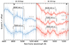 |
Fig. 11. Fe II triplet λλ4923, 5018, 5169 region of SN 2020xga (left panel) at −8.3 and +37.8 day spectra and SN 2022xgc at +21.9, +65.5 and +92.1 days spectra. A normalization and an arbitrary offset has been applied for illustration purposes. The spectra have been smoothed using the Savitzky-Golay filter and the original data are shown in lighter colors. The absorption features that correspond to the blueshift of the Fe II lines are denoted along with the velocities. |
In Fig. 11, in the spectrum of SN 2022xgc we resolved three absorption lines that we identify as Fe IIλλ4924, 5018, 5169. At +21.9 days the troughs match with a ejecta velocity of ∼8100 km s−1, though the mismatch of the absorption at 4940 Å can be explained by a blend of Fe II with other ions. The triplet is better resolved in the spectra at +65.4 and +92.1 days and the velocity decreases by ∼1000 km s−1 within 70 days.
To compare these values with the ZTF sample, we plot in Fig. 12 the velocity evolution of 38 ZTF SLSNe-I with Fe II velocities, together with the velocity evolution of SN 2020xga and SN 2022xgc. The value of ∼8000 km s−1 measured from the pre-peak spectrum of SN 2020xga is lower than what we find in the ZTF sample, but not unprecedented since there are at least two SLSNe within ±20 days after the peak in the ZTF sample with Fe II velocities close to 8000 km s−1. In SN 2022xgc, the first measurement of the velocity is derived from the spectrum at +21.9 days following the peak. At this phase, the estimated value of 8100 km s−1 is within the velocity range of the ZTF sample at similar phases but lower than the bulk of the population. Both objects appear to evolve slower than the ZTF sample.
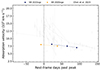 |
Fig. 12. Fe II ejecta velocities of SN 2020xga and SN 2022xgc as measured from the X-shooter spectra as a function of time. The velocity evolution of the ZTF SLSN-I sample is shown in gray for comparison. The vertical dash-dotted line illustrates the phase of the maximum light. |
4.4. Comparison with other hydrogen-poor superluminous supernovae
In Sect. 3.1, we compared the photometric properties of SN 2020xga and SN 2022xgc with the homogeneous ZTF sample (Chen et al. 2023a) and found that the light curve characteristics of SN 2020xga and SN 2022xgc are either average or span across the entire distribution, aside being very bright. However, SN 2020xga and SN 2022xgc display a spectroscopic signature rarely seen in SLSN-I spectra, and thus we seek to compare the spectra of SN 2020xga and SN 2022xgc with those of typical SLSNe-I.
In Fig. 13 (left), we compare the X-shooter spectra of SN 2020xga and SN 2022xgc at −8.3 and +37.8, and +21.9, +65.4 and +92.1 days after the peak, respectively, with a sample of well-studied SNe from the literature including PTF09cnd (Quimby et al. 2011, 2018), LSQ12dlf (Nicholl et al. 2014) and SN 2015bn (Nicholl et al. 2016). As was previously indicated, the pre-peak spectrum of SN 2020xga shows a strong O II series, similar to the one found in PTF09cnd, albeit the absorption components in PTF09cnd are shifted to higher velocities compared to the ones in SN 2020xga. The O II lines are also seen in the spectrum of SN 2015bn at the same phase as the pre-peak spectrum of SN 2020xga, although they are weaker than for SN 2020xga and PTF09cnd. The O II lines are not clearly seen in the spectra of SN 2022xgc and LSQ12dlf during the early photospheric phase, which could be explained by the fact that the conditions for O II excitation may not satisfied (e.g., Mazzali et al. 2016; Dessart 2019; Könyves-Tóth 2022; Saito et al. 2024).
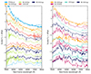 |
Fig. 13. Spectral comparison of SN 2020xga and SN 2022xgc with SLSNe-I from the literature. Left: Comparison of SN 2020xga and SN 2022xgc spectra with typical well-studied SLSNe-I at similar epochs. Right: SN 2020xga and SN 2022xgc spectra in comparison with SLSNe-I that display the second narrow Mg II absorption system. All spectra are corrected for MW extinction and have been smoothed using a Savitzky-Golay filter. |
As the ejecta cool, the spectra of SN 2020xga and SN 2022xgc become similar to those of type Ic SNe at maximum, as anticipated for the typical SLSNe-I. Overall, the general shape of the spectra of SN 2020xga and SN 2022xgc both pre- and post-peak are similar to the spectra of typical SLSNe-I and do not present any unusual spectral properties aside the second narrow Mg II absorption system in the UV part of the spectrum, which is further discussed in Sect. 5. We note that in the spectra of SN 2020xga and SN 2022xgc more features are resolved than often seen in spectra of typical SLSNe-I, due to the high signal and good resolution of the X-shooter data.
In Fig. 13 (right), we compare the X-shooter spectra of SN 2020xga and SN 2022xgc with the spectra of SN 2018ibb and iPTF16eh at similar phases. SN 2020xga is the only object in this class that displays strong O II lines; the O II W-shape appears to be present in iPTF16eh but weaker than in SN 2020xga. In the spectra of SN 2022xgc and SN 2018ibb the Fe II triplet is resolved though the Fe IIλ5018 in the spectrum of SN 2022xgc at +21.9 days does not align with the absorption component. In contrast to SN 2020xga and iPTF16eh, which do not exhibit any obvious feature in the red part of the optical spectrum in the spectra near peak, both SN 2022xgc and SN 2018ibb show strong Si IIλ6355. As the temperature drops and elements from deeper inside are revealed, the spectra of all these objects become similar to those of standard type Ic SNe. However, SN 2018ibb (Schulze et al. 2024) develops features such as [O II], [O III], and [Ca II] at the early photospheric phase that are not common for SNe. The spectroscopic peculiarity along with the outstanding light curve timescales make SN 2018ibb a unique SLSN-I, which stands out even among the SLSNe-I that display the rare signature of the second Mg II system (Schulze et al. 2024).
5. Circumstellar material shell around SN 2020xga and SN 2022xgc
5.1. Modeling of the Mg II absorption lines
The X-shooter spectra of SN 2020xga and SN 2022xgc at −8.3 and +21.9 days, respectively, show two Mg II absorption systems. The positive identification of the second system as Mg II is supported by the absence of other transitions from the SN ejecta and the characteristic separation between the Mg II doublet components. In Fig. 14 a zoom-in region around the Mg II lines at ∼2800 Å of SN 2020xga and SN 2022xgc is presented in velocity space. The narrow Mg II systems at zero rest-frame velocity originate from the ISM of the host galaxies and are used for the determination of the SN redshift (see Sect. 4.1). The blueshifted Mg II systems are significantly broader (270 km s−1 for SN 2020xga and 500 km s−1 for SN 2022xgc) than expected for the ISM in dwarf host galaxies (Krühler et al. 2015; Arabsalmani et al. 2018) but also narrower compared to the SN features (> 1000 km s−1). This supports the hypothesis that these systems arise from fast-moving absorbing gas that is not part of the ejecta or the host galaxy. The only objects that showed such lines are iPTF16eh and SN 2018ibb and they have been associated with the existence of a rapidly expanding CSM shell expelled a few years before the SN explosion (Lunnan et al. 2018b). We rule out the possibility that the Mg II absorption reflects a peculiar composition of the ejecta, as this would require unusually high Mg abundances, in which case O and Ne lines would also be present in the spectra (Woosley et al. 2002).
 |
Fig. 14. X-shooter spectra of SN 2020xga at −8.3 days (top panel) and SN 2022xgc at +21.9 days (bottom panel). The spectra show resolved, narrow absorption lines from the host ISM (marked by the vertical dashed orange lines) and a blueshifted absorption line system (marked by the vertical dashed purple lines) from a CSM shell expelled shortly before the SN explosion. |
To estimate the distance and the thickness of the CSM shell, we modeled the line profile of the Mg II doublet using a modified Monte Carlo scattering code. While the line profile from a spherically symmetric shell for a single scattering line can be calculated analytically (Fransson 1984), the doublet nature of the Mg II lines will cause scattering from the blue component by the red component that affects the line profiles. We therefore used a Monte Carlo code to model the line profile, based on the Monte Carlo code in Fransson et al. (2014) and Taddia et al. (2020), used for type IIn SNe. We assumed that the photons around 2800 Å produced in the SN “photosphere” are scattered by an expanding spherical shell with an inner radius of Rin and an outer radius of Rout. The scattering is assumed to be coherent and isotropic in the frame of the expanding shell. In reality, the background “continuum” is produced by lines from the expanding ejecta, most likely dominated by the broad Mg II lines (Sect. 4). We assumed that this continuum is given by the observed spectrum at velocities larger than that of the shell, and adjusted the background spectrum so that the total spectrum, “continuum” plus the scattered emission from the shell agreed with the observations. At the observed absorption velocity of the shell, the “continuum” flux was simply interpolated. Since there is no indication of thermal emission from the shell (contrary to the case of iPTF 16eh, Lunnan et al. 2018b), we neglected collisional excitation for the line profile, as well as other NLTE effects. Given that our primary interest is in the kinematics of the shell, which is only observed in the Mg II lines, a more detailed NLTE treatment is not justified. We did not include scattering by the thermal motions of the electrons, as the electron scattering depth of the shell should be small, and there are no indications of smooth, extended wings of the lines in our best S/N spectrum (Fig. 15), as is discussed in Hillier (1991).
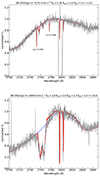 |
Fig. 15. Modeling on the Mg II doublets originating from the CSM shell (broad features) and the ISM of the host galaxy (narrow features) for SN 2020xga (top) and SN 2022xgc (bottom). The observed spectrum in the 2800 Å region is presented in gray and the best model fit is shown in red. The dashed blue line illustrates the SN continuum. For SN 2020xga we have marked the CaH [MYAMP] K lines from the MW. |
We assumed that the expansion of the shell is homologous with V = Vmax(r/Rout), which is reasonable for a time-limited eruption, such as PPI or LBV eruptions. This configuration gives rise to the second Mg II system from the shell, which we observe as an emission and/or absorption lines on top of the SN photospheric flux. The homologous assumption is expected to break down when the fast moving ejecta catches up with the slower shell and hydrodynamically interacts. This is expected to either heat the shell to X-ray temperatures and ionize Mg almost completely, or, if it would radiatively cool, produce flat topped emission lines. There is no evidence for either case.
We assumed that the CSM is mainly characterized by an optical depth τ of the shell. In the Sobolev approximation (Sobolev 1957) this is for a homologous expansion given by
 (5)
(5)
Here, A21 = 2.8 × 10⁸ s−1 is the transition rate between the upper level 2 and lower level 1, n1 is the number density in the ground state, λ the wavelength, g1 = 2 and g2 the statistical weights of the lower and upper levels, respectively, and t the time from the eruption. For the 2795.5 Å line g2 = 4 and for the 2802.7 Å line g2 = 2. The relative depth of the blue and red Mg II doublet can be used to determine the optical depth. In the optically thin limit this ratio is 2.0, decreasing as the optical depth increases.
The shell is assumed to have a constant density, or, more precisely, a constant optical depth. Since the shells we are considering are geometrically thin, variations in density, such as a wind-like distribution where ρ ∝ r−2, are expected to have only a minor effect. Although this is a simplification, it is reasonable given the uncertainty in the details of the ejection process, such as the mass loss history during the eruption. In particular, the inner and outer radii of the shell should not be sensitive to this assumption.
The velocity range of the absorption from the shell gives a direct measure of the radial extent of the shell. For a homologous expansion of the shell and for a single line the minimum, Vblue and maximum, Vred, velocity of the absorption is given by
![Mathematical equation: $$ \begin{aligned} V_{\rm blue}&= -V_{\rm max}\nonumber \\ V_{\rm red}&= -V_{\rm max} \left(\frac{R_{\rm in}}{R_{\rm out}}\right)^\alpha \left[1 - \left(\frac{R_{\rm phot}}{R_{\rm in}}\right)^2\right]^{1/2}. \end{aligned} $$](/articles/aa/full_html/2025/02/aa52357-24/aa52357-24-eq49.gif) (6)
(6)
For homologous expansion, α = 1, and for a constant velocity shell, α = 0. Determining the maximum and minimum velocities of the absorption we can therefore estimate the Rin and Rout of the shell relative to the photospheric radius. We note that the minimum velocity of the shell is not −Vred, but Vin = Rin/t. While we have here assumed homologous expansion, a shell with constant velocity only differs marginally in a slightly lower velocity unless the shell is very broad. The absorption line profile, however, differs from the homologous, lacking a flat bottom at the minimum absorption and instead being more V-shaped (see e.g., Figs. 4 and 5 in Fransson 1984). The observed absorption profiles for SN 2022xgc (Fig. 14) argue against a constant velocity shell, but is compatible with a homologous expansion. This is also the case for SN 2020xga (Fig. 14) and SN 2018ibb (see Sect. 5.2), although the S/N makes this conclusion marginal.
For homologous expansion, Eq. (6) can be inverted to show that
![Mathematical equation: $$ \begin{aligned} \frac{R_{\rm in}}{R_{\rm out}} = \left[\left(\frac{V_{\rm red}}{V_{\rm blue}}\right)^2 + \left(\frac{R_{\rm phot}}{R_{\rm out}}\right)^2\right]^{1/2}. \end{aligned} $$](/articles/aa/full_html/2025/02/aa52357-24/aa52357-24-eq50.gif) (7)
(7)
The relative thickness of the shell, and therefore the depth of the absorption, decreases as the radius of the shell increases. The depth of the absorption therefore provides a constraint on the radius of the shell.
Figure 15 shows the observed data for SN 2020xga and SN 2022xgc around the 2800 Å region along with the modeled Mg II line profiles. For SN 2020xga there is good agreement between the model and the observations for Rin = 2.96 Rphot and Rout = 3.00 Rphot, where Rphot is the photospheric radius, and Vmax = 4275 km s−1. Using the blackbody radius we derived in Sect. 3.2 from the given observed spectrum, we estimate that the CSM shell is located at 1.29 ± 0.01 × 1016 cm and extends to 1.31 ± 0.01 × 1016 cm. The emission for the CSM shell is weak and consistent with the SN continuum. Given the derived distance of the shell and the estimated maximum velocity of 4275 km s−1, the shell was expelled  months before the core collapse, assuming a constant shell velocity as is seen in the case of SN 2018ibb.
In SN 2022xgc the best-fit model is for a CSM shell with properties of Rin = 1.8 Rphot, Rout = 2.0 Rphot, Vmax = 4400 km s−1. This leads to a shell extending from 7.96 ± 0.03 × 1015 cm to 8.84 ± 0.03 × 1015 cm. Contrary to SN 2020xga, the emission from the CSM shell in SN 2022xgc is well above the SN continuum (dashed red line) and contributes significantly to the shape of the output spectra around the 2800 Å region. This is a result of the considerably broader CSM shell, which scatter a larger fraction of the photons outside the absorption lines. Utilizing the maximum velocity of 4400 km s−1 calculated by the absorption minima of the broad Mg II lines and assuming that the shell has not been decelerated, we estimate the time of CSM ejection to be  months before the SN explosion. We caution that the error bars in the time of ejection reflect only statistical uncertainties and do not account for any systematic errors that may arise from uncertainties in the explosion date. However, uncertainties of a few days in the explosion date will not affect significantly the results.
The relative depth of the blue and red Mg II doublet in SN 2020xga indicate an optical depth of τ ≈ 0.5. Using Δr = (Vout − Vin)t for a homologous shell one finds for the column density of Mg II, N = n1Δr,
 (8)
(8)
which is also valid for large τ. For SN 2020xga, we find N(Mg II) ∼ 4.7 × 1012 cm−2. The uncertainty in τ, and therefore N(Mg II), is at least a factor of two. In the case of SN 2022xgc the lines are saturated with τ > 5 and we only find a lower limit of N(Mg II) > 4.7 × 1014 cm−2.
In both SN 2020xga and SN 2022xgc, the X-shooter spectra obtained at later epochs are very noisy in the UV part of the spectrum that we are interested in and any potential Mg II lines from the CSM shell cannot be resolved. Thus, we are not able to track the evolution of the Mg II line profiles, which could provide a hint about the geometry of the shell. We note that for this part of the analysis we used only the spectra obtained through our X-shooter program due to the high S/N and the particular sensitivity of the instrument in the bluer wavelengths.
5.2. Comparison with similar hydrogen-poor superluminous supernovae
Figure 16 shows a zoom-in of the Mg II region of all the four objects that have shown the high velocity CSM absorption systems. The Mg II doublets originating from the CSM have various shapes and are shifted by various velocities reflecting the diversity of the CSM shells located around the SLSNe. In iPTF16eh the broad Mg II lines are blueshifted by 3300 km s−1 and in SN 2018ibb by 2918 km s−1 indicating shells moving somewhat slower but still comparable to the ones in SN 2020xga and SN 2022xgc. The Mg II doublet in SN 2020xga is shallower compared to the rest of the objects, which supports the idea that a CSM in SN 2020xga is placed at larger radius with respect to its photosphere in comparison to the other three objects showing this signature in their spectra. On the other hand, the deep and blended Mg II lines in SN 2022xgc and iPTF16eh points toward broader CSM shells in comparison to SN 2020xga and SN 2018ibb.
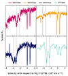 |
Fig. 16. Comparison of the broad Mg II lines originating from the CSM shells for SN 2020xga, SN 2022xgc, SN 2018ibb and iPTF 16eh. The spectra are corrected for MW extinction. The vertical black lines mark the velocity of the absorption minima of the secondary Mg II lines. |
Motivated by the above analysis for SN 2020xga and SN 2022xgc, we modeled the Mg II doublet line profile of SN 2018ibb (Schulze et al. 2024) using the X-shooter spectrum at +32.7 days after maximum to quantify the properties of the CSM shell (see Fig. 17). The best fit model is for a CSM shell with Rin = 2.00 Rphot, Rout = 2.14 Rphot and Vmax = 3200 km s−1. Using the photospheric-radius values reported in Schulze et al. (2024), we calculated a shell extended from 1.00 ± 0.05 × 1016 cm out to 1.07 ± 0.05 × 1016 cm. Similarly to SN 2022xgc, the emission from the shell contributes significantly to the spectrum of SN 2018ibb around the 2800 Å region. Using Eq. (8) we estimated the lower limit to the column density of Mg II in the CSM shell of SN 2018ibb to be N(Mg II) ∼ 9.2 × 1013 cm−2, in agreement with the value derived in Schulze et al. (2024). Finally, we estimated the time of the CSM expelling to be < 9 months before the core collapse given the high uncertainty of the explosion date in SN 2018ibb.
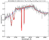 |
Fig. 17. Modeling on the Mg II doublets originated from the CSM shell (broad features) and the ISM of the host galaxy (narrow features) for SN 2018ibb. The observed spectrum at the 2800 Å region is presented in gray and the best model fit in red. The dashed blue line illustrates the SN continuum. |
In iPTF16eh (Lunnan et al. 2018b, see their Fig. 1), an intermediate-width Mg II emission appeared at ∼2800 Å approximately 100 days after explosion and was persistent for more than 200 days. During this timescale, the line centroid was shifting from −1600 km s−1 to 2900 km s−1, while the FWHM remained constant. This time- and wavelength-dependant emission line was associated with a resonance scattering light echo from a CSM shell. In the case of iPTF16eh, due to the low-resolution spectrum, the Mg II scattered shell emission was modeled instead to estimate the size and the thickness of the CSM. Lunnan et al. (2018b) find that the shell is located at ∼3.37 × 1017 cm, extended out to ∼3.55 × 1017 cm and was expelled ∼30 years before explosion. The CSM radius of iPTF16eh is almost an order of magnitude higher than the one derived from the modeling of SN 2020xga and SN 2022xgc. The evolution of the emerging Mg II emission line in iPTF16eh was used as diagnostic for the geometry of the shell, which according to Lunnan et al. (2018b) is found to be roughly spherical. Motivated by this study, Schulze et al. (2024) analyzed the spectra of SN 2018ibb between +230 and +378 days after the peak and detected Mg II in emission. However, due to heavy rebinning of the data, it is uncertain whether this emission line is connected with light echo from the CSM shell. In SN 2020xga and SN 2022xgc, we do not observe any variable Mg II in emission; thus, we cannot derive any conclusion about the geometry of the shell.
6. Host galaxy properties
6.1. Host galaxy of SN 2020xga
In Fig. 8 (left panel), two Mg II and Fe II absorption systems are resolved in the host galaxy of SN 2020xga. As is discussed in Sect. 4.1, the stronger system is at z = 0.4283 and the weaker one at z = 0.4296, with a velocity separation of ∼260 km s−1. These two absorbing systems could arise either as a consequence of gas cloud motions (infall or outflows of gas) in the host galaxy or from a neighboring galaxy intervening in the line of sight (e.g., Ledoux et al. 2006; Chen 2012; Møller et al. 2013; Friis et al. 2015). Since the emission lines from the star-forming regions are centered on a redshift in between the absorption components (z = 0.4287) and the velocity separation of ∼260 km s−1 is the typical difference in rotational velocity in a galaxy (Galbany et al. 2016), the scenario of mapping different regions of a single host galaxy is more likely (Friis et al. 2015).
The determination of the SN redshift in this case in not straightforward. Vreeswijk et al. (2014) showed that the absorbing gas responsible for the narrow lines in the spectrum of the SLSN iPTF 13ajg was produced by gas in the ISM located at least 50 pc from the SN. In addition, Friis et al. (2015), which presented a similar picture to SN 2020xga in terms of the lines of the GRB 121024A host galaxy, found that the absorbing clouds are not probing the actual GRB environment, but rather gas that has been photoionized by the GRB out to hundreds of parsecs. Although there are some distinctions between GRB and SLSN host galaxies (e.g., Vreeswijk et al. 2014; Lunnan et al. 2014; Ørum et al. 2020), both are tracers of star formation, and therefore the assumption that the SN redshift is same as the redshift of the emission lines would not be unreasonable. Alternatively, to break the redshift degeneracy we would need high-resolution imaging and spectroscopy of the host galaxy to resolve the morphology of the galaxy and to infer the SN location and measure the redshift of that location. However, since analyzing the host environment of SN 2020xga is out of the scope of this paper and the redshift values are different only in the third digit, we take as the redshift of the SN the highest value. We note that considering the redshift of the emission lines or the strong Mg II system would not affect our analysis and would not change significantly the results inferred from the CSM modeling.
6.2. Stellar population synthesis modeling
To infer the mass and SFR of the host of SN 2020xga, we modeled the observed SED built from the broadband photometry (Table 1) and the measured emission lines (Table 4) with the software package PROSPECTOR (Johnson et al. 2021) version 1.114. We assumed a Chabrier initial mass function (IMF; Chabrier 2003) and approximated the star formation history (SFH) by a linearly increasing SFH at early times followed by an exponential decline at late times (functional form t × exp(−t/t1/e), where t is the age of the SFH episode and t1/e is the e-folding timescale). The model was attenuated with the Calzetti model (Calzetti et al. 2000). The priors of the model parameters were set to be identical to the ones used by Schulze et al. (2021). The observed SED is adequately described by a galaxy model with a stellar mass of log  and SFR of
  yr−1 (gray curve in Fig. 18), leading to a specific SFR of 10−8 yr−1. The values derived from the modeling of SN 2020xga are consistent with what is seen in the host galaxies of other SLSNe-I (Perley et al. 2016; Angus et al. 2019; Schulze et al. 2021).
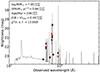 |
Fig. 18. Spectral energy distribution of the host galaxy of SN 2020xga (black data points). The solid line displays the best-fitting model of the SED. The red squares represent the model-predicted magnitudes. The fitting parameters are shown in the upper-left corner. The abbreviation ‘n.o.f.’ stands for the number of filters. |
6.3. Emission line diagnostics
Using the narrow emission lines from the galaxy present in the X-shooter spectra of SN 2020xga at +37.8 days and SN 2022xgc at +21.9 days, we can derive some properties of the two SLSN hosts regarding their metallicity, SFR, and host galaxy extinction. After calibrating the spectra to the photometry and correcting for MW extinction, we measured the fluxes of the emission lines utilizing the python package LIME (Fernández et al. 2024). The resulting flux values are listed in Table 4.
Observed host galaxy emission line fluxes of SN 2020xga and SN 2022xgc.
We used the Balmer decrement to measure the host galaxy extinction of SN 2020xga, and found a value of Hα/Hβ = 2.3 ± 0.9, which is consistent within the uncertainty with the theoretical ratio of 2.87 for no extinction (assuming Case B recombination and a temperature of 10 000 K; Osterbrock & Ferland 2006); thus we did not apply any host galaxy extinction correction to the SN 2020xga photometry. In the spectrum of SN 2022xgc only the Hα line was detected, thus we cannot estimate the extinction of SN 2022xgc’s host.
The SFR can be derived from the luminosity of Hα emission line using the Kennicutt (1998) relation and the relation from Madau & Dickinson (2014) to convert from the Salpeter to the Chabrier IMF in the Kennicutt (1998). This gives a SFR of 0.24 ± 0.03 M⊙ yr−1 for SN 2020xga and 0.009 ± 0.003 M⊙ yr−1 for SN 2022xgc assuming zero host extinction. The value for SN 2020xga is lower than what is inferred from the SED modeling but not unprecedented compared to what is seen among SLSN host galaxies, while the value for SN 2022xgc points toward a ultra-faint dwarf galaxy (e.g., Perley et al. 2016; Angus et al. 2016).
Since we do not detect the auroral line [O III] λ4363 in the spectrum of SN 2020xga, we are limited to strong-line metallicity diagnostics, such as R23, O3N2, or N2 (Pagel et al. 1979; Pettini & Pagel 2004; see discussion in Kewley & Ellison 2008). The O3N2 and N2 indexes require the [N II] line flux that evaded detection. Thus, we used the R23 index with the calibrations of Jiang et al. (2019), and the non-detection of [N II] to break the degeneracy. We calculated for SN 2020xga  dex. Taking the solar value to be 12 + log(O/H)⊙ = 8.69 dex (Asplund et al. 2021), this corresponds to a metallicity Z = 0.2 Z⊙. The metallicity of SN 2020xga is in agreement with the values reported for other SLSN-I host galaxies (< 0.5 Z⊙; e.g., Lunnan et al. 2014; Leloudas et al. 2015; Perley et al. 2016; Chen et al. 2017; Schulze et al. 2018). We do not derive any metallicity measurement for the host of SN 2022xgc due to the lack of detection of emission lines originating from the host galaxy in the spectrum of SN 2022xgc.
7. Discussion
7.1. The origin of the circumstellar material
In Sect. 5, we modeled the broad Mg II lines in the spectra of SN 2022xgc and SN 2020xga originating from CSM shells located around the SNe. The question that we need to address is what process led to the ejection of the material that generated the CSM at this distance and these velocities. Our findings indicate that this material was expelled less than a year before the core collapse in the final stages of stellar evolution, supporting a scenario of eruptive mass loss, since line-driven winds have much longer timescales than the evolutionary timescales at the post-MS phase.
One scenario to explain the detected CSM shells is the giant eruptions of LBV stars. The best observed example is the “Great Eruption” of η Carinae in 1843 in which 12 − 20 M⊙ (or more; Smith et al. 2003) of material was ejected within a decade, moving at velocities between 650 − 6000 km s−1 (Davidson et al. 2001; Currie et al. 2002; Smith 2002, 2008; Smith & Morse 2004). The geometry of ejecta-nebulae in LBV eruptions can be very anisotropic, as is observed in η Carinae. Although the causes of LBV eruptions are still unknown, several theories have been proposed (e.g., Davidson 1987; Owocki et al. 2004; Smith et al. 2003; Smith 2006, 2008; Woosley 2017; Akashi & Kashi 2020; Cheng et al. 2024).
For iPTF16eh, Lunnan et al. (2018b) did not exclude an LBV-like eruption as a possibility for the formation of the CSM shell located around the SN. However, the spherically detached shell seen in iPTF16eh is not consistent with the asymmetric CSM structure may be expected in this type of eruption (see Fig. 1 in Smith 2008). Since in the spectra of SN 2022xgc and SN 2020xga the shell velocities of ∼4000 km s−1 are consistent with an LBV-related eruption and the geometry of the shells cannot be constrained (see Sect. 5), previous massive ejection such as that in an LBV cannot be ruled out.
The LBV eruptions have also been discussed that could be driven by the PPI mechanism (Woosley 2017), which occurs for a He core in the mass range of 30 − 65 M⊙ (Woosley et al. 2007). For the PPI, the primary parameter determining the duration between the shell ejections and the ultimate core collapse, as well as the expelled mass and their kinetic energy, is the mass of the He core MHe (Woosley 2017; Leung et al. 2019; Marchant et al. 2019). The time interval could range from a few hours up to 10 000 years. For MHe < 40 − 42 M⊙, the energy released is insufficient to unbind significant amounts of material, resulting in multiple weak pulses (Woosley 2017; Renzo et al. 2020), whereas for MHe > 50 M⊙, the time delay between strong pulses becomes long, forming shells at distances greater than the photospheric radius of the SN (Woosley 2017). We note that the PPI scenario is addressed in relation to the mechanism responsible for forming the observed CSM shells, rather than as a powering mechanism for SN 2020xga and SN 2022xgc (see discussion in Sect. 7.4).
For SN 2020xga, the CSM was estimated to be expelled ∼11 months before the SN explosion. This value corresponds to that of a pure He core of 51 M⊙ with no rotation and zero metallicity in the study of Woosley (2017). Exploring the models of Woosley (2017) for the blue supergiant progenitors developed using the KEPLER code (Weaver et al. 1978; Weaver & Woosley 1993; Woosley et al. 2002), we found that the model best describing the observed CSM properties of SN 2020xga is the B105. Assuming that the material in the B105 model has been ejected in one strong pulse ∼2 years before the core collapse, at the time of the detection, the shell is moving at ∼2700 km s−1 at a radius of about 1.8 × 1016 cm. The shell velocity derived from Woosley (2017) model is substantially lower than our prediction, but its distance is comparable to our estimated value for SN 2020xga. The model B100, on the other hand, has slightly higher velocity, but at the moment of detection, the shell is four times closer to the SN than in our model. We note that the exploration of these models focuses on the properties of the CSM shell resulting from their ejection, and we do not intend to directly link these models to the light curve properties of SN 2020xga and SN 2022xgc.
The discrepancy between the observed properties of the CSM and the predicted CSM properties from Woosley (2017) models may stem from our assumption that the material was ejected in a single pulse, which is unlikely for stars of these masses (see Table 1 in Woosley 2017; Marchant et al. 2019). However, assuming that the models must have at least one pulse on a time-scale equivalent to the ejection time of the CSM shell we observed, we could set a lower limit on the stellar mass. Thus, in SN 2020xga given that the shell was ejected ∼11 months before the core collapse, the mass of the progenitor should be > 51 M⊙ for zero metallicity, within this framework. The lower limit corresponds to the case in which the CSM was formed in the first pulses. An upper limit is harder to set because it is closely related to the energetics of the PPI, the number of pulses and the timescales between the pulses; however, if restricted by the PPI regime it must be < 62 M⊙.
A similar comparison can be done with the H-free low metallicity models developed by Marchant et al. (2019) with the MESA software (Paxton et al. 2011, 2013, 2015, 2018). In this study, the limit goes down to 47 M⊙ presumably due to the fact that the models of Marchant et al. (2019) consider mass loss by stellar winds. This value is consistent with the modeling of Renzo et al. (2020) (see their Table C.1), and the shell velocities resulting from their simulations can be similar to the ones found in the spectrum of SN 2020xga.
A comparable analysis for SN 2022xgc indicates that the predicted ejection timeframe of ∼5 months corresponds to the model with > 50 M⊙ of pure He core (Woosley 2017) for zero metallicity, and > 46 M⊙ when low metallicity is taken into consideration. However, given the variations in the shell velocities in SN 2020xga and SN 2022xgc, and therefore in the energetics, the properties of the progenitor stars of SN 2020xga and SN 2022xgc are likely to be different. According to Renzo et al. (2020), even a difference of only 0.2 M⊙ across the models may result in distinct PPI characteristics.
As is discussed in Leung et al. (2019), there are substantial quantitative differences for the same He core mass between the models of Woosley (2017), Marchant et al. (2019) and by extension Renzo et al. (2020), including ejected masses and time intervals between the pulses that can be traced back to the treatment of shocks and convection. We note that none of the aforementioned models have been constructed to match the observable CSM properties of SN 2020xga and SN 2022xgc and that tuning is required to obtain better estimates for the shell properties; however, a qualitative comparison could provide some limits for the mass of the progenitor star that undergoes PPI before the final SN explosion. The threshold for the He-core progenitor mass could be further reduced if rotation is considered, as the induced chemical mixing could enable the formation of the required He-core in lower-mass stars compared to nonrotating models (Chatzopoulos et al. 2012; Woosley 2017).
The discussion of SN 2018ibb in the context of PPI is challenging as it is considered the best candidate of a PISN (Schulze et al. 2024). PISN can be the end fate for stars with He cores between 65 − 130 M⊙ (Heger & Woosley 2002), where the energy produced by the pair creation obliterates the entire star. There are no models of PI SNe that also show eruptions similar to the PPI SNe, although this needs further investigations. However, Schulze et al. (2024) supports the presence of a CSM shell surrounding SN 2018ibb based on the spectroscopic signs of interaction between the ejecta and the shell. The presence of CSM in SN 2018ibb was also supported by our modeling in Sect. 5. The formation of CSM shells has been discussed by Schulze et al. (2024) in the context of an LBV-like eruption analogous to the one in η Carinae.
To strengthen the hypothesis of eruptive mass loss in SN 2020xga and SN 2022xgc, we analyzed the available ATLAS and ZTF forced photometry between 400 days pre-explosion and the time of explosion, paying particular attention to the estimated timeframes of the mass ejections to see if there is any detection. In SN 2022xgc, the time of eruption falls into the gap owing to the solar conjunction, therefore we cannot detect any light from the putative blast. In the case of SN 2020xga, we were unable to find any meaningful detection at ∼10 months before explosion, but merely upper limits, implying that the eruption was probably fainter than the detection limits. Strotjohann et al. (2021) searched systematically for precursor eruptions hundreds of days before the explosion in a sample of SNe at z < 0.14. Their sample include one SLSN-II with z ≈ 0.20 in which a precursor is detected; however, Strotjohann et al. (2021) mentioned that at this progenitor distance the activity is more likely associated with AGN rather than stellar flares. Thus, it is not surprising that we do not detect any activity in the light curve prior to the explosion of SN 2020xga and SN 2022xgc given the distances of these two objects (z = 0.4296 and z = 0.3103).
The analysis of the four SLSNe that exhibit the broad Mg II absorption system, revealing the existence of a CSM shell expelled less than a year before the core collapse, has demonstrated that determining the expelling mechanism is challenging because various mechanisms could result in the formation of CSM at such distances. One possible hint to distinguish the various eruptive mass loss mechanisms could be to constrain the geometry of the CSM shells. In the future, improved modeling of the very final moments of massive stars will be necessary to comprehend the star’s late activity and the mechanisms that lead to the formation of the CSM shells.
7.2. When the ejecta will interact with the circumstellar material shell
As is discussed throughout the paper, the second Mg II absorption system in the spectra of SN 2020xga and SN 2022xgc is explained by resonance-line scattering of the SLSN background photospheric emission by a rapidly expanding CSM shell located at a few 1016 cm. To calculate the time of interaction tint of the ejecta with the fast moving material, we assume that the inner radius of the shell is equal to the distance covered by the outer layer of ejecta. This is given by
 (9)
(9)
where Vej, max is the velocity of the outer layer of the ejecta, terup is the time of eruption before explosion, and Vin is the minimum velocity of the shell (see definition in Sect. 5). From the spectra of SN 2020xga, we measure a maximum ejecta velocity of ∼13 000 km s−1 using the O II lines. Using the predicted value for Rin in Sect. 5 for the spectra at −8.3 days, we calculated the Vin = 4210 km s−1. Thus, from Eq. (9) we computed that the ejecta will collide with the CSM  days after explosion and
  days after maximum, provided that the rise of the light curve from the first light is
  days. We do not have any spectroscopic or photometric observation at the time of collision to detect any possible interaction signature in SN 2020xga.
Following the same technique for SN 2022xgc, and measuring a maximum velocity of 11 500 km s−1 from the Fe II triplet and Vin = 3960 km s−1, we estimated a collision time of  days after the explosion. Given that the rise from the time of first light is
  days, the ejecta will interact with the CSM
  days after maximum. This suggests that when we obtained the X-shooter spectra +21.9 days after the peak, the ejecta had more likely already begun interacting with the CSM shell. In addition, in Fig. 4 the blackbody radius of SN 2022xgc at +55 days after the peak is 1 × 1016 cm, similar to the radius of the CSM, strengthening the hypothesis that the ejecta have interacted with the CSM at the time of our observations. We do not see any emerging emission line in the spectra of SN 2022xgc, that could have offered information on the CSM interaction; however, this could be due to the fact that the spectral lines are highly sensitive to the density profiles of the ejecta and the CSM (e.g., Fransson 1984; Chevalier & Fransson 2017; Chatzopoulos et al. 2012). Furthermore, the polarimetry of SN 2022xgc does not reveal any evidence of asymmetry that may come from the interaction of the ejecta with the CSM shell, which we anticipate to have happened during the period of time covered by the polarimetry (+26.1 days and +60.1 days after the peak). The effect of the CSM interaction might start becoming visible at around 80 post-peak days at which the light curve of SN 2022xgc (see Fig. 2) shows a potential flattening in the gcr filters. We should highlight that the computed time of interaction for SN 2020xga and SN 2022xgc should be taken with caution since it is highly dependent on the (uncertain) maximum velocity and the explosion date.
Motivated by the above discussion for SN 2020xga and SN 2022xgc, we conducted the same calculations for SN 2018ibb to check whether our predicted values are consistent with the timescales stated in Schulze et al. (2024). Using the maximum velocity reported in Schulze et al. (2024) of 12 500 km s−1 and the estimated Rin, we found that the ejecta of SN 2018ibb is predicted to interact with the CSM ∼90 days after explosion. The rise time of the SN 2018ibb is > 93 days, implying the interaction occurred during the rise. The light curve of SN 2018ibb shows bumps and undulations in various bands post peak. Furthermore, the [Ca II] emission line, which was already present in the spectrum of SN 2018ibb at −1.4 days, and the [O II] and [O III] emission lines appear approximately +30 days after maximum light, has been associated with the CSM shell. These timescales agree with our predicted interaction time.
7.3. The composition and mass of the circumstellar material shells
The determination of the chemical composition of the CSM shells in SN 2020xga and SN 2022xgc is hampered by a lack of observations. In SN 2020xga, we do not have observational data at our estimated time of interaction, while for SN 2022xgc, even though we found that the ejecta had already started interacting with the CSM shell at the time we obtained the spectra, there are no spectroscopic interaction signatures such as narrow emission lines. This does not necessarily imply that the CSM of SN 2022xgc is H-, He-, and O-free; rather, the evidence of interaction has yet to be revealed.
The Mg II doublet lines that we observed from the CSM are one of the few resonance lines of abundant elements in the observed part of the spectrum along with the Ca IIλλ3968.5, 4226.7, the Na Iλλ5890.0, 5895.9 and the K Iλλ7664.9, 7699.0 (Morton 2003). Due to the fact that Na I and K I have a low ionization potential, and Ca is less abundant and has a lower ionization potential than Mg, these lines are ionized by the SN continuum. Thus, it is not surprising that we observe only the Mg II doublet from the CSM. The far-UV rest frame below ∼2000 Å contains a large number of resonance lines, as well as intercombination lines of abundant ions such as CII-IV, NII-V, OI-IV, which could be used for a more constraining abundance determination. This would, however, require either observations with HST or a SLSN at considerably higher redshift.
Assuming that the CSM shell of SN 2020xga and SN 2022xgc are H-dominated and using the same method as in Lunnan et al. (2018b), we could put an upper limit on the H mass of the shell by utilizing the luminosity of Hα. We assumed that the CSM Hα peak is blueshifted from the host Hα by the velocity of the CSM measured from the Mg II doublet and that the line profile of the CSM Hα is similar to the estimated Mg II emission one extended to the maximum velocity of the CSM Mg II absorption. We found that LHα < 1.8 × 1038 erg s−1 and LHα < 1.2 × 1039 erg s−1 for SN 2020xga and SN 2022xgc,, respectively. This yields a limit of Mshell < 0.03f0.5 M⊙ for SN 2020xga and Mshell < 0.02f0.5 M⊙ for SN 2022xgc where f is the filling factor. These CSM masses are substantially lower than the values for ejected masses expected in Woosley (2017), Marchant et al. (2019), and Renzo et al. (2020), indicating that the shell is most likely not dominated by H and that the H envelope must have been lost before this eruption. This is also evident in SN 2018ibb in which the absence of H and He lines throughout the entire spectral evolution of SN 2018ibb and the existence of O lines suggests that the CSM shell must be O-dominated and any H and He must reside at much larger radii (Schulze et al. 2024).
7.4. What powers SN 2020xga and SN 2022xgc
In Sect. 3.4, we modeled the light curves of SN 2020xga and SN 2022xgc with the REDBACK software, assuming they are powered by a magnetar. The modeling resulted in very rapidly spinning magnetars (1.6 and 0.9 ms, respectively) with ejecta masses of 7 − 9 M⊙, consistent with what is seen in SLSNe-I (Chen et al. 2023b; Gomez et al. 2024). However, the spin period in the case of SN 2020xga and SN 2022xgc approaches the mass-shedding limit (Watts et al. 2016), which suggests that in order to explain the very high luminosities observed in SN 2020xga and SN 2022xgc with the magnetar model, the magnetar must produce energy near to its upper limits without being destabilized.
A remaining question is how a star more massive than ∼50 M⊙ can explode with ∼9 M⊙ of ejecta. The stars massive enough to satisfy the PPI conditions form Fe cores, which tend to collapse rather than explode (e.g., Heger & Woosley 2002). However, Woosley et al. (2007) discuss a possibility in which a massive star (with initial mass of ∼95 M⊙) with mild rotation and magnetic torques may have enough angular momentum in its Fe core to form a NS with a period of 2 ms. Furthermore, Woosley (2017) investigated the explosions of numerous PPI models, including the model of a 50 M⊙ He-core, and discovered that the light curve produced is compatible with observations of some of the brightest SLSNe-I and therefore, in accordance with the observables of SN 2020xga and SN 2022xgc. In the case of the formation of a NS, Lunnan et al. (2018b) argue that the magnetic field must be > 1015 G initially to allow the star to explode, but then it must decay to < 1014 G to power the light curve for longer timescales. This scenario would require a high level of fine-tuning in the rotation of the star since it is expected to have a key part in the star’s final death and consequently in the SN explosion.
Alternative scenarios include SN 2020xga and SN 2022xgc being PPISNe, or powered by fallback accretion into a black hole or CSM interaction. The observed radiated energies of > 1.8 × 1051 erg and > 0.9 × 1051 erg for SN 2020xga and SN 2022xgc, respectively, cannot be reproduced by the PPISN scenario because the maximum energy of the pure PPISN models is ∼5 × 1050 erg unless there is a contribution from a magnetar (Woosley 2017). The fallback scenario proposes that the star only partially explodes, resulting in a weak SN explosion and fallback accretion on the equatorial plane (e.g., Dexter & Kasen 2013; Woosley 2017; Moriya et al. 2018). While the fallback material is accreted onto the black hole, the resulting outflows can come in the form of disk winds or jets and they may interact with previously ejected material, causing a significant impact in the SLSN-I light curves. We fit the light curves of SN 2020xga and SN 2022xgc with the fallback model from Moriya et al. (2018). Assuming an 100% accretion efficiency, we would need 5 M⊙ of accreted mass to power both SN 2020xga and SN 2022xgc. Assuming a more realistic efficiency of 10−3 (Moriya et al. 2018) would require an accreted mass of 5000 M⊙, which we deem unrealistic. The efficiency could be on the order of 10% if a jet is formed (Gilkis et al. 2016), implying an accretion mass of 50 M⊙. This would be consistent with the “missing” ejecta in the PPI scenario of SN 2020xga and SN 2022xgc. However, there is no evidence of a jet in our data (see Sect. 3.5 for SN 2022xgc). Nevertheless, given the low ejecta mass inferred from the relatively short rise times of the light curves of SN 2020xga and SN 2022xgc, the fallback accretion scenario cannot be ruled out as a plausible powering mechanism.
Finally, we explored the scenario in which SN 2020xga and SN 2022xgc are powered by the interaction of the ejecta with CSM. We modeled the light curves using REDBACK and the CSM+Ni (Chatzopoulos et al. 2012) model, and found that the ejecta and CSM masses range from 1 − 3 M⊙ and 35 − 50 M⊙, respectively. While these findings may seem unphysical, they are not unprecedented, as semianalytic models (Chatzopoulos et al. 2012) and hydrodynamic simulations (Moriya et al. 2013, 2018; Sorokina et al. 2016) have shown to yield conflicting results. The development of consistent radiation-hydrodynamic simulations is necessary to properly model the light curves of SLSNe-I, similar to what has be done in Dessart et al. (2015). However, considering that these stars expel material prior to their explosion, and particularly in the case of SN 2022xgc, the presence of the three early r-band data points, along with the fact that the ejecta is estimated to have interacted with the CSM during our observations, we conclude that CSM interaction could contribute to the light curves of SN 2020xga and SN 2022xgc.
Determining the powering mechanism of the light curves of SLSNe-I is still an open question and especially in the high mass ranges in which the “explodability” is highly uncertain (e.g., Ertl et al. 2016; Coughlin et al. 2018; see discussion in Renzo et al. 2020). Our observations put limitations on any progenitor model by requiring a significant mass ejections less than a few years before explosion.
8. Conclusions
In this work, we provide optical observations of the H-poor SLSNe-I SN 2020xga and SN 2022xgc covering −44 to +59 and −59 to +110 days after maximum light, respectively. Our key findings are as follows:
-
SN 2020xga and SN 2022xgc are among the most luminous SLSNe-I, with Mg = −22.3 mag and Mg = −22.0 mag, respectively.
-
The spectra of SN 2020xga and SN 2022xgc show a second Mg II absorption system coming from the CSM surrounding the SNe, but are otherwise similar to the spectra of normal SLSNe-I.
-
The modeling of the narrow Mg II results in a CSM shell for SN 2020xga located at ∼1.3 × 1016 cm and for SN 2022xgc located at ∼0.8 × 1016 cm moving at maximum velocity of 4275 km s−1 and 4400 km s−1, respectively.
-
The CSM shells of SN 2020xga and SN 2022xgc were expelled less than a year before the core collapse as a result of eruptive-mass loss in the form of LBV-like eruptions or PPI.
-
The light curve modeling of SN 2020xga and SN 2022xgc is consistent with magnetar-powered SNe with an ejecta mass of about ∼7 − 9 M⊙ with magnetars near the mass-shedding limit.
-
The PPI scenario suggests He cores > 50 M⊙, which is incompatible with the findings of the light curve modeling; hence, alternatives such as fallback accretion and CSM interaction are discussed.
-
The host galaxy properties of SN 2020xga and SN 2022xgc are similar to the ones of typical SLSN-I host galaxies and point toward dwarf galaxies.
In this paper, we focus on the extensive analysis of two objects that show the spectroscopic signature of the presence of a CSM shell expelled less than a year before the core collapse. The analysis of the whole high-quality X-shooter spectral sample constraining the fraction of SLSNe that show evidence of eruptive mass loss and establishing observational limitations will be addressed in a future work. The discovery of these objects can provide an insight into the late stages of stellar evolution as well as a better knowledge of SLSN-I progenitors.
Data availability
The photometric data for SN 2020xga and SN 2022xgc are available at the CDS via anonymous ftp to cdsarc.cds.unistra.fr (130.79.128.5) or via https://cdsarc.cds.unistra.fr/viz-bin/cat/J/A+A/694/A292. All spectra of SN 2020xga and SN 2022xgc have been uploaded to the WISeREP15 archive (Yaron & Gal-Yam 2012). The corner plots of SN 2020xga and SN 2022xgc resulting from the REDBACK modeling are available at https://zenodo.org/records/14565605.
Reported in Transient Name Server.
PROSPECTOR uses the FLEXIBLE STELLAR POPULATION SYNTHESIS [FSPS] code (Conroy et al. 2009) to generate the underlying physical model and PYTHON-FSPS (Foreman-Mackey et al. 2014) to interface with FSPS in PYTHON. The FSPS code also accounts for the contribution from the diffuse gas based on the CLOUDY models from (Byler et al. 2017). We use the dynamic nested sampling package DYNESTY (Speagle 2020) to sample the posterior probability.
References
- Aamer, A., Nicholl, M., Jerkstrand, A., et al. 2024, MNRAS, 527, 11970 [Google Scholar]
- Ahn, C. P., Alexandroff, R., Allende Prieto, C., et al. 2012, ApJS, 203, 21 [Google Scholar]
- Akashi, M., & Kashi, A. 2020, MNRAS, 494, 3186 [NASA ADS] [CrossRef] [Google Scholar]
- Ambikasaran, S., Foreman-Mackey, D., Greengard, L., Hogg, D. W., & O’Neil, M. 2015, IEEE Trans. Pattern Anal. Mach. Intell., 38, 252 [Google Scholar]
- Angus, C. R., Levan, A. J., Perley, D. A., et al. 2016, MNRAS, 458, 84 [NASA ADS] [CrossRef] [Google Scholar]
- Angus, C. R., Smith, M., Sullivan, M., et al. 2019, MNRAS, 487, 2215 [NASA ADS] [CrossRef] [Google Scholar]
- Arabsalmani, M., Møller, P., Perley, D. A., et al. 2018, MNRAS, 473, 3312 [NASA ADS] [CrossRef] [Google Scholar]
- Arcavi, I. 2022, ApJ, 937, 75 [CrossRef] [Google Scholar]
- Arnett, W. D., & Fu, A. 1989, ApJ, 340, 396 [NASA ADS] [CrossRef] [Google Scholar]
- Ashton, G., Hübner, M., Lasky, P. D., et al. 2019, ApJS, 241, 27 [NASA ADS] [CrossRef] [Google Scholar]
- Asplund, M., Amarsi, A. M., & Grevesse, N. 2021, A&A, 653, A141 [NASA ADS] [CrossRef] [EDP Sciences] [Google Scholar]
- Barkat, Z., Rakavy, G., & Sack, N. 1967, Phys. Rev. Lett., 18, 379 [Google Scholar]
- Bellm, E. C., Kulkarni, S. R., Graham, M. J., et al. 2019, PASP, 131, 018002 [Google Scholar]
- Blagorodnova, N., Neill, J. D., Walters, R., et al. 2018, PASP, 130, 035003 [Google Scholar]
- Blanchard, P. K., Berger, E., Nicholl, M., & Villar, V. A. 2020, ApJ, 897, 114 [NASA ADS] [CrossRef] [Google Scholar]
- Branch, D., Benetti, S., Kasen, D., et al. 2002, ApJ, 566, 1005 [NASA ADS] [CrossRef] [Google Scholar]
- Brennan, S. J., & Fraser, M. 2022, A&A, 667, A62 [NASA ADS] [CrossRef] [EDP Sciences] [Google Scholar]
- Buzzoni, B., Delabre, B., Dekker, H., et al. 1984, The Messenger, 38, 9 [NASA ADS] [Google Scholar]
- Byler, N., Dalcanton, J. J., Conroy, C., & Johnson, B. D. 2017, ApJ, 840, 44 [Google Scholar]
- Calzetti, D., Armus, L., Bohlin, R. C., et al. 2000, ApJ, 533, 682 [NASA ADS] [CrossRef] [Google Scholar]
- Chabrier, G. 2003, PASP, 115, 763 [Google Scholar]
- Chambers, K. C., Magnier, E. A., Metcalfe, N., et al. 2016, ArXiv e-prints [arXiv:1612.05560] [Google Scholar]
- Chambers, K. C., Boer, T. D., Bulger, J., et al. 2020, Transient Name Server Discovery Report, 2020-3164, 1 [Google Scholar]
- Chatzopoulos, E., & Wheeler, J. C. 2012a, ApJ, 748, 42 [NASA ADS] [CrossRef] [Google Scholar]
- Chatzopoulos, E., & Wheeler, J. C. 2012b, ApJ, 760, 154 [NASA ADS] [CrossRef] [Google Scholar]
- Chatzopoulos, E., Wheeler, J. C., & Vinko, J. 2012, ApJ, 746, 121 [Google Scholar]
- Chen, H.-W. 2012, MNRAS, 419, 3039 [NASA ADS] [CrossRef] [Google Scholar]
- Chen, T.-W., Smartt, S. J., Bresolin, F., et al. 2013, ApJ, 763, L28 [NASA ADS] [CrossRef] [Google Scholar]
- Chen, T. W., Smartt, S. J., Jerkstrand, A., et al. 2015, MNRAS, 452, 1567 [NASA ADS] [CrossRef] [Google Scholar]
- Chen, T.-W., Smartt, S. J., Yates, R. M., et al. 2017, MNRAS, 470, 3566 [NASA ADS] [CrossRef] [Google Scholar]
- Chen, Z. H., Yan, L., Kangas, T., et al. 2023a, ApJ, 943, 41 [NASA ADS] [CrossRef] [Google Scholar]
- Chen, Z. H., Yan, L., Kangas, T., et al. 2023b, ApJ, 943, 42 [NASA ADS] [CrossRef] [Google Scholar]
- Cheng, S. J., Goldberg, J. A., Cantiello, M., et al. 2024, ApJ, 974, 270 [NASA ADS] [CrossRef] [Google Scholar]
- Chevalier, R. A., & Fransson, C. 2017, in Handbook of Supernovae, eds. A. W. Alsabti, & P. Murdin, 875 [Google Scholar]
- Chomiuk, L., Chornock, R., Soderberg, A. M., et al. 2011, ApJ, 743, 114 [NASA ADS] [CrossRef] [Google Scholar]
- Conroy, C., Gunn, J. E., & White, M. 2009, ApJ, 699, 486 [Google Scholar]
- Coughlin, E. R., Quataert, E., Fernández, R., & Kasen, D. 2018, MNRAS, 477, 1225 [NASA ADS] [CrossRef] [Google Scholar]
- Coughlin, M. W., Bloom, J. S., Nir, G., et al. 2023, ApJS, 267, 31 [NASA ADS] [CrossRef] [Google Scholar]
- Currie, D. G., Dorland, B. N., & Kaufer, A. 2002, A&A, 389, L65 [NASA ADS] [CrossRef] [EDP Sciences] [Google Scholar]
- Davidson, K. 1987, ApJ, 317, 760 [NASA ADS] [CrossRef] [Google Scholar]
- Davidson, K., Smith, N., Gull, T. R., Ishibashi, K., & Hillier, D. J. 2001, AJ, 121, 1569 [Google Scholar]
- De Cia, A., Gal-Yam, A., Rubin, A., et al. 2018, ApJ, 860, 100 [NASA ADS] [CrossRef] [Google Scholar]
- Dekany, R., Smith, R. M., Riddle, R., et al. 2020, PASP, 132, 038001 [NASA ADS] [CrossRef] [Google Scholar]
- Dessart, L. 2019, A&A, 621, A141 [NASA ADS] [CrossRef] [EDP Sciences] [Google Scholar]
- Dessart, L., Hillier, D. J., Waldman, R., Livne, E., & Blondin, S. 2012, MNRAS, 426, L76 [NASA ADS] [CrossRef] [Google Scholar]
- Dessart, L., Audit, E., & Hillier, D. J. 2015, MNRAS, 449, 4304 [Google Scholar]
- Dexter, J., & Kasen, D. 2013, ApJ, 772, 30 [NASA ADS] [CrossRef] [Google Scholar]
- Dey, A., Schlegel, D. J., Lang, D., et al. 2019, AJ, 157, 168 [Google Scholar]
- Ergon, M., Sollerman, J., Pursimo, T., et al. 2013, ATel, 4912, 1 [NASA ADS] [Google Scholar]
- Ertl, T., Janka, H. T., Woosley, S. E., Sukhbold, T., & Ugliano, M. 2016, ApJ, 818, 124 [NASA ADS] [CrossRef] [Google Scholar]
- Fernández, V., Amorín, R., Firpo, V., & Morisset, C. 2024, A&A, 688, A69 [NASA ADS] [CrossRef] [EDP Sciences] [Google Scholar]
- Fiore, A., Chen, T. W., Jerkstrand, A., et al. 2021, MNRAS, 502, 2120 [NASA ADS] [CrossRef] [Google Scholar]
- Fitzpatrick, E. L. 1999, PASP, 111, 63 [Google Scholar]
- Flewelling, H. A., Magnier, E. A., Chambers, K. C., et al. 2020, ApJS, 251, 7 [NASA ADS] [CrossRef] [Google Scholar]
- Foreman-Mackey, D., Sick, J., & Johnson, B. 2014, https://doi.org/10.5281/zenodo.12157 [Google Scholar]
- Fransson, C. 1984, A&A, 132, 115 [NASA ADS] [Google Scholar]
- Fransson, C., Ergon, M., Challis, P. J., et al. 2014, ApJ, 797, 118 [Google Scholar]
- Fremling, C. 2022, Transient Name Server Discovery Report, 2022-2935, 1 [Google Scholar]
- Fremling, C., Sollerman, J., Taddia, F., et al. 2016, A&A, 593, A68 [NASA ADS] [CrossRef] [EDP Sciences] [Google Scholar]
- Friis, M., De Cia, A., Krühler, T., et al. 2015, MNRAS, 451, 167 [NASA ADS] [CrossRef] [Google Scholar]
- Fuller, J., & Ro, S. 2018, MNRAS, 476, 1853 [NASA ADS] [CrossRef] [Google Scholar]
- Galbany, L., Anderson, J. P., Rosales-Ortega, F. F., et al. 2016, MNRAS, 455, 4087 [NASA ADS] [CrossRef] [Google Scholar]
- Gal-Yam, A. 2012, Science, 337, 927 [Google Scholar]
- Gal-Yam, A. 2019a, ApJ, 882, 102 [NASA ADS] [CrossRef] [Google Scholar]
- Gal-Yam, A. 2019b, ARA&A, 57, 305 [Google Scholar]
- Gilkis, A., Soker, N., & Papish, O. 2016, ApJ, 826, 178 [NASA ADS] [CrossRef] [Google Scholar]
- Gkini, A., Lunnan, R., Schulze, S., et al. 2024, A&A, 685, A20 [NASA ADS] [CrossRef] [EDP Sciences] [Google Scholar]
- Goldoni, P., Royer, F., François, P., et al. 2006, SPIE Conf. Ser., 6269, 62692K [Google Scholar]
- Gomez, S., Nicholl, M., Berger, E., et al. 2024, MNRAS, 535, 471 [NASA ADS] [CrossRef] [Google Scholar]
- Götberg, Y., de Mink, S. E., & Groh, J. H. 2017, A&A, 608, A11 [NASA ADS] [CrossRef] [EDP Sciences] [Google Scholar]
- Graham, M. J., Kulkarni, S. R., Bellm, E. C., et al. 2019, PASP, 131, 078001 [Google Scholar]
- Gromadzki, M., Ihanec, N., Moran, S., & Yaron, O. 2020, Transient Name Server Classification Report, 2020-3372, 1 [Google Scholar]
- Gromadzki, M., Grzesiak, K., Kravtsov, T., et al. 2022, Transient Name Server AstroNote, 253, 1 [NASA ADS] [Google Scholar]
- Grzesiak, K., Gromadzki, M., Kravtsov, T., et al. 2022, Transient Name Server AstroNote, 255, 1 [NASA ADS] [Google Scholar]
- Gutiérrez, C. P., Pastorello, A., Bersten, M., et al. 2022, MNRAS, 517, 2056 [CrossRef] [Google Scholar]
- Heger, A., & Woosley, S. E. 2002, ApJ, 567, 532 [Google Scholar]
- Heiles, C. 2000, AJ, 119, 923 [Google Scholar]
- Hillier, D. J. 1991, A&A, 247, 455 [NASA ADS] [Google Scholar]
- Hsu, B., Hosseinzadeh, G., & Berger, E. 2021, ApJ, 921, 180 [CrossRef] [Google Scholar]
- Humphreys, R. M. 1999, in IAU Colloq. 169: Variable and Non-spherical Stellar Winds in Luminous Hot Stars, eds. B. Wolf, O. Stahl, & A. W. Fullerton, 523, 243 [NASA ADS] [CrossRef] [Google Scholar]
- Ihanec, N., Gromadzki, M., Moran, S., et al. 2020, Transient Name Server AstroNote, 220, 1 [NASA ADS] [Google Scholar]
- Inserra, C., Smartt, S. J., Jerkstrand, A., et al. 2013, ApJ, 770, 128 [NASA ADS] [CrossRef] [Google Scholar]
- Inserra, C., Nicholl, M., Chen, T. W., et al. 2017, MNRAS, 468, 4642 [NASA ADS] [CrossRef] [Google Scholar]
- Jiang, T., Malhotra, S., Rhoads, J. E., & Yang, H. 2019, ApJ, 872, 145 [NASA ADS] [CrossRef] [Google Scholar]
- Johnson, B. D., Leja, J., Conroy, C., & Speagle, J. S. 2021, ApJS, 254, 22 [NASA ADS] [CrossRef] [Google Scholar]
- Kaiser, N., Burgett, W., Chambers, K., et al. 2010, SPIE Conf. Ser., 7733, 77330E [Google Scholar]
- Kasen, D. 2017, in Handbook of Supernovae, eds. A. W. Alsabti, & P. Murdin, 939 [Google Scholar]
- Kasen, D., & Bildsten, L. 2010, ApJ, 717, 245 [NASA ADS] [CrossRef] [Google Scholar]
- Kennicutt, R. C. 1998, ApJ, 498, 541 [NASA ADS] [CrossRef] [Google Scholar]
- Kewley, L. J., & Ellison, S. L. 2008, ApJ, 681, 1183 [Google Scholar]
- Kim, Y. L., Rigault, M., Neill, J. D., et al. 2022, PASP, 134, 024505 [NASA ADS] [CrossRef] [Google Scholar]
- Kleiser, I. K. W., & Kasen, D. 2014, MNRAS, 438, 318 [Google Scholar]
- Könyves-Tóth, R. 2022, ApJ, 940, 69 [CrossRef] [Google Scholar]
- Kramida, A., Ralchenko, Yu., Reader, J., & and NIST ASD Team 2022, NIST Atomic Spectra Database (ver. 5.10), https://physics.nist.gov/asd [Google Scholar]
- Krühler, T., Malesani, D., Fynbo, J. P. U., et al. 2015, A&A, 581, A125 [Google Scholar]
- Lamers, H. J. G. L. M., Haser, S., de Koter, A., & Leitherer, C. 1999, ApJ, 516, 872 [CrossRef] [Google Scholar]
- Laplace, E., Götberg, Y., de Mink, S. E., Justham, S., & Farmer, R. 2020, A&A, 637, A6 [NASA ADS] [CrossRef] [EDP Sciences] [Google Scholar]
- Ledoux, C., Petitjean, P., Fynbo, J. P. U., Møller, P., & Srianand, R. 2006, A&A, 457, 71 [NASA ADS] [CrossRef] [EDP Sciences] [Google Scholar]
- Leloudas, G., Chatzopoulos, E., Dilday, B., et al. 2012, A&A, 541, A129 [NASA ADS] [CrossRef] [EDP Sciences] [Google Scholar]
- Leloudas, G., Schulze, S., Krühler, T., et al. 2015, MNRAS, 449, 917 [NASA ADS] [CrossRef] [Google Scholar]
- Leung, S.-C., Nomoto, K., & Blinnikov, S. 2019, ApJ, 887, 72 [Google Scholar]
- Leung, S.-C., Wu, S., & Fuller, J. 2021, ApJ, 923, 41 [NASA ADS] [CrossRef] [Google Scholar]
- Liu, Y.-Q., Modjaz, M., & Bianco, F. B. 2017, ApJ, 845, 85 [NASA ADS] [CrossRef] [Google Scholar]
- Lucy, L. B., & Solomon, P. M. 1970, ApJ, 159, 879 [Google Scholar]
- Lunnan, R., Chornock, R., Berger, E., et al. 2014, ApJ, 787, 138 [NASA ADS] [CrossRef] [Google Scholar]
- Lunnan, R., Chornock, R., Berger, E., et al. 2016, ApJ, 831, 144 [NASA ADS] [CrossRef] [Google Scholar]
- Lunnan, R., Chornock, R., Berger, E., et al. 2018a, ApJ, 852, 81 [NASA ADS] [CrossRef] [Google Scholar]
- Lunnan, R., Fransson, C., Vreeswijk, P. M., et al. 2018b, Nat. Astron., 2, 887 [NASA ADS] [CrossRef] [Google Scholar]
- Lupton, R., Blanton, M. R., Fekete, G., et al. 2004, PASP, 116, 133 [NASA ADS] [CrossRef] [Google Scholar]
- Lyman, J. D., Bersier, D., & James, P. A. 2014, MNRAS, 437, 3848 [Google Scholar]
- Madau, P., & Dickinson, M. 2014, ARA&A, 52, 415 [Google Scholar]
- Marchant, P., Renzo, M., Farmer, R., et al. 2019, ApJ, 882, 36 [Google Scholar]
- Masci, F. J., Laher, R. R., Rusholme, B., et al. 2019, PASP, 131, 018003 [Google Scholar]
- Mazzali, P. A., Sullivan, M., Pian, E., Greiner, J., & Kann, D. A. 2016, MNRAS, 458, 3455 [NASA ADS] [CrossRef] [Google Scholar]
- Metzger, B. D., Margalit, B., Kasen, D., & Quataert, E. 2015, MNRAS, 454, 3311 [NASA ADS] [CrossRef] [Google Scholar]
- Modigliani, A., Goldoni, P., Royer, F., et al. 2010, SPIE Conf. Ser., 7737, 773728 [Google Scholar]
- Modjaz, M., Liu, Y. Q., Bianco, F. B., & Graur, O. 2016, ApJ, 832, 108 [NASA ADS] [CrossRef] [Google Scholar]
- Møller, P., Fynbo, J. P. U., Ledoux, C., & Nilsson, K. K. 2013, MNRAS, 430, 2680 [CrossRef] [Google Scholar]
- Moriya, T. J., Maeda, K., Taddia, F., et al. 2013, MNRAS, 435, 1520 [CrossRef] [Google Scholar]
- Moriya, T. J., Nicholl, M., & Guillochon, J. 2018, ApJ, 867, 113 [NASA ADS] [CrossRef] [Google Scholar]
- Morton, D. C. 2003, ApJS, 149, 205 [Google Scholar]
- Neill, J. D., Sullivan, M., Gal-Yam, A., et al. 2011, ApJ, 727, 15 [NASA ADS] [CrossRef] [Google Scholar]
- Nicholl, M., Smartt, S. J., Jerkstrand, A., et al. 2013, Nature, 502, 346 [NASA ADS] [CrossRef] [Google Scholar]
- Nicholl, M., Smartt, S. J., Jerkstrand, A., et al. 2014, MNRAS, 444, 2096 [NASA ADS] [CrossRef] [Google Scholar]
- Nicholl, M., Smartt, S. J., Jerkstrand, A., et al. 2015a, MNRAS, 452, 3869 [NASA ADS] [CrossRef] [Google Scholar]
- Nicholl, M., Smartt, S. J., Jerkstrand, A., et al. 2015b, ApJ, 807, L18 [NASA ADS] [CrossRef] [Google Scholar]
- Nicholl, M., Berger, E., Smartt, S. J., et al. 2016, ApJ, 826, 39 [NASA ADS] [CrossRef] [Google Scholar]
- Nicholl, M., Guillochon, J., & Berger, E. 2017, ApJ, 850, 55 [NASA ADS] [CrossRef] [Google Scholar]
- Oke, J. B., & Gunn, J. E. 1982, PASP, 94, 586 [Google Scholar]
- Omand, C. M. B., & Sarin, N. 2024, MNRAS, 527, 6455 [Google Scholar]
- Ørum, S. V., Ivens, D. L., Strandberg, P., et al. 2020, A&A, 643, A47 [NASA ADS] [CrossRef] [EDP Sciences] [Google Scholar]
- Osterbrock, D. E., & Ferland, G. J. 2006, Astrophysics of Gaseous Nebulae and Active Galactic Nuclei (Sausalito: University Science Books) [Google Scholar]
- Ostriker, J. P., & Gunn, J. E. 1971, ApJ, 164, L95 [NASA ADS] [CrossRef] [Google Scholar]
- Owocki, S. P., Gayley, K. G., & Shaviv, N. J. 2004, ApJ, 616, 525 [NASA ADS] [CrossRef] [Google Scholar]
- Pagel, B. E. J., Edmunds, M. G., Blackwell, D. E., Chun, M. S., & Smith, G. 1979, MNRAS, 189, 95 [NASA ADS] [CrossRef] [Google Scholar]
- Pastorello, A., Smartt, S. J., Botticella, M. T., et al. 2010, ApJ, 724, L16 [NASA ADS] [CrossRef] [Google Scholar]
- Paxton, B., Bildsten, L., Dotter, A., et al. 2011, ApJS, 192, 3 [Google Scholar]
- Paxton, B., Cantiello, M., Arras, P., et al. 2013, ApJS, 208, 4 [Google Scholar]
- Paxton, B., Marchant, P., Schwab, J., et al. 2015, ApJS, 220, 15 [Google Scholar]
- Paxton, B., Schwab, J., Bauer, E. B., et al. 2018, ApJS, 234, 34 [NASA ADS] [CrossRef] [Google Scholar]
- Perley, D. A., Quimby, R. M., Yan, L., et al. 2016, ApJ, 830, 13 [NASA ADS] [CrossRef] [Google Scholar]
- Perley, D. A., Fremling, C., Sollerman, J., et al. 2020, ApJ, 904, 35 [NASA ADS] [CrossRef] [Google Scholar]
- Petrović, J. 2020, Serb. Astron. J., 201, 1 [CrossRef] [Google Scholar]
- Petrovic, J., Langer, N., & van der Hucht, K. A. 2005, A&A, 435, 1013 [NASA ADS] [CrossRef] [EDP Sciences] [Google Scholar]
- Pettini, M., & Pagel, B. E. J. 2004, MNRAS, 348, L59 [NASA ADS] [CrossRef] [Google Scholar]
- Piro, A. L. 2015, ApJ, 808, L51 [NASA ADS] [CrossRef] [Google Scholar]
- Planck Collaboration VI. 2020, A&A, 641, A6 [NASA ADS] [CrossRef] [EDP Sciences] [Google Scholar]
- Poidevin, F., Pérez-Fournon, I., Delgado-González, Z., et al. 2022, Transient Name Server Classification Report, 2022-3523, 1 [Google Scholar]
- Prochaska, J., Hennawi, J., Westfall, K., et al. 2020a, J. Open Source Softw., 5, 2308 [NASA ADS] [CrossRef] [Google Scholar]
- Prochaska, J. X., Hennawi, J., Cooke, R., et al. 2020b, https://doi.org/10.5281/zenodo.3743493 [Google Scholar]
- Puls, J., Vink, J. S., & Najarro, F. 2008, A&ARv, 16, 209 [NASA ADS] [CrossRef] [Google Scholar]
- Pursiainen, M., Leloudas, G., Paraskeva, E., et al. 2022, A&A, 666, A30 [NASA ADS] [CrossRef] [EDP Sciences] [Google Scholar]
- Pursiainen, M., Leloudas, G., Cikota, A., et al. 2023, A&A, 674, A81 [NASA ADS] [CrossRef] [EDP Sciences] [Google Scholar]
- Quataert, E., & Shiode, J. 2012, MNRAS, 423, L92 [NASA ADS] [CrossRef] [Google Scholar]
- Quimby, R. M., Kulkarni, S. R., Kasliwal, M. M., et al. 2011, Nature, 474, 487 [NASA ADS] [CrossRef] [Google Scholar]
- Quimby, R. M., De Cia, A., Gal-Yam, A., et al. 2018, ApJ, 855, 2 [Google Scholar]
- Rakavy, G., & Shaviv, G. 1967, ApJ, 148, 803 [Google Scholar]
- Renzo, M., Farmer, R., Justham, S., et al. 2020, A&A, 640, A56 [NASA ADS] [CrossRef] [EDP Sciences] [Google Scholar]
- Rigault, M., Neill, J. D., Blagorodnova, N., et al. 2019, A&A, 627, A115 [NASA ADS] [CrossRef] [EDP Sciences] [Google Scholar]
- Saito, S., Tanaka, M., Mazzali, P. A., Hachinger, S., & Hotokezaka, K. 2024, ApJ, 967, 13 [CrossRef] [Google Scholar]
- Sarin, N., Omand, C. M. B., Margalit, B., & Jones, D. I. 2022, MNRAS, 516, 4949 [Google Scholar]
- Sarin, N., Hübner, M., Omand, C. M. B., et al. 2024, MNRAS, 531, 1203 [NASA ADS] [CrossRef] [Google Scholar]
- Schlafly, E. F., & Finkbeiner, D. P. 2011, ApJ, 737, 103 [Google Scholar]
- Schulze, S., Krühler, T., Leloudas, G., et al. 2018, MNRAS, 473, 1258 [NASA ADS] [CrossRef] [Google Scholar]
- Schulze, S., Yaron, O., Sollerman, J., et al. 2021, ApJS, 255, 29 [NASA ADS] [CrossRef] [Google Scholar]
- Schulze, S., Fransson, C., Kozyreva, A., et al. 2024, A&A, 683, A223 [NASA ADS] [CrossRef] [EDP Sciences] [Google Scholar]
- Selsing, J., Malesani, D., Goldoni, P., et al. 2019, A&A, 623, A92 [NASA ADS] [CrossRef] [EDP Sciences] [Google Scholar]
- Serkowski, K., Mathewson, D. S., & Ford, V. L. 1975, ApJ, 196, 261 [NASA ADS] [CrossRef] [Google Scholar]
- Shingles, L., Smith, K. W., Young, D. R., et al. 2021, Transient Name Server AstroNote, 7, 1 [NASA ADS] [Google Scholar]
- Shiode, J. H., & Quataert, E. 2014, ApJ, 780, 96 [Google Scholar]
- Silverman, J. M., Foley, R. J., Filippenko, A. V., et al. 2012, MNRAS, 425, 1789 [Google Scholar]
- Smartt, S. J., Valenti, S., Fraser, M., et al. 2015, A&A, 579, A40 [NASA ADS] [CrossRef] [EDP Sciences] [Google Scholar]
- Smith, N. 2002, MNRAS, 337, 1252 [NASA ADS] [CrossRef] [Google Scholar]
- Smith, N. 2006, ApJ, 644, 1151 [Google Scholar]
- Smith, N. 2008, Nature, 455, 201 [Google Scholar]
- Smith, N. 2014, ARA&A, 52, 487 [NASA ADS] [CrossRef] [Google Scholar]
- Smith, N., & Arnett, W. D. 2014, ApJ, 785, 82 [NASA ADS] [CrossRef] [Google Scholar]
- Smith, N., & Morse, J. A. 2004, ApJ, 605, 854 [NASA ADS] [CrossRef] [Google Scholar]
- Smith, N., Gehrz, R. D., Hinz, P. M., et al. 2003, AJ, 125, 1458 [NASA ADS] [CrossRef] [Google Scholar]
- Smith, M., Sullivan, M., D’Andrea, C. B., et al. 2016, ApJ, 818, L8 [NASA ADS] [CrossRef] [Google Scholar]
- Smith, K. W., Smartt, S. J., Young, D. R., et al. 2020, PASP, 132, 085002 [Google Scholar]
- Sobolev, V. V. 1957, Soviet Ast., 1, 678 [NASA ADS] [Google Scholar]
- Sorokina, E., Blinnikov, S., Nomoto, K., Quimby, R., & Tolstov, A. 2016, ApJ, 829, 17 [NASA ADS] [CrossRef] [Google Scholar]
- Speagle, J. S. 2020, MNRAS, 493, 3132 [Google Scholar]
- Steele, I. A., Smith, R. J., Rees, P. C., et al. 2004, SPIE Conf. Ser., 5489, 679 [Google Scholar]
- Strotjohann, N. L., Ofek, E. O., Gal-Yam, A., et al. 2021, ApJ, 907, 99 [NASA ADS] [CrossRef] [Google Scholar]
- Suzuki, A., & Maeda, K. 2021, ApJ, 908, 217 [NASA ADS] [CrossRef] [Google Scholar]
- Taddia, F., Stritzinger, M. D., Fransson, C., et al. 2020, A&A, 638, A92 [NASA ADS] [CrossRef] [EDP Sciences] [Google Scholar]
- Taggart, K., & Perley, D. A. 2021, MNRAS, 503, 3931 [NASA ADS] [CrossRef] [Google Scholar]
- Thomas, R. C., Nugent, P. E., & Meza, J. C. 2011, PASP, 123, 237 [NASA ADS] [CrossRef] [Google Scholar]
- Tonry, J. L., Denneau, L., Heinze, A. N., et al. 2018, PASP, 130, 064505 [Google Scholar]
- Tonry, J., Denneau, L., Heinze, A., et al. 2020, Transient Name Server Discovery Report, 2020-3392, 1 [Google Scholar]
- van der Walt, S., Crellin-Quick, A., & Bloom, J. 2019, J. Open Source Softw., 4, 1247 [NASA ADS] [CrossRef] [Google Scholar]
- van Dokkum, P. G. 2001, PASP, 113, 1420 [Google Scholar]
- Vernet, J., Dekker, H., D’Odorico, S., et al. 2011, A&A, 536, A105 [NASA ADS] [CrossRef] [EDP Sciences] [Google Scholar]
- Vreeswijk, P. M., Savaglio, S., Gal-Yam, A., et al. 2014, ApJ, 797, 24 [NASA ADS] [CrossRef] [Google Scholar]
- Vreeswijk, P. M., Leloudas, G., Gal-Yam, A., et al. 2017, ApJ, 835, 58 [NASA ADS] [CrossRef] [Google Scholar]
- Vurm, I., & Metzger, B. D. 2021, ApJ, 917, 77 [NASA ADS] [CrossRef] [Google Scholar]
- Wang, L., Wheeler, J. C., & Höflich, P. 1997, ApJ, 476, L27 [NASA ADS] [CrossRef] [Google Scholar]
- Watts, A. L., Andersson, N., Chakrabarty, D., et al. 2016, Rev. Mod. Phys., 88, 021001 [NASA ADS] [CrossRef] [Google Scholar]
- Weaver, T. A., & Woosley, S. E. 1993, Phys. Rep., 227, 65 [Google Scholar]
- Weaver, T. A., Zimmerman, G. B., & Woosley, S. E. 1978, ApJ, 225, 1021 [NASA ADS] [CrossRef] [Google Scholar]
- Westphal, J. A., & Neugebauer, G. 1969, ApJ, 156, L45 [NASA ADS] [CrossRef] [Google Scholar]
- Wheeler, J. C., Chatzopoulos, E., Vinkó, J., & Tuminello, R. 2017, ApJ, 851, L14 [NASA ADS] [CrossRef] [Google Scholar]
- Woosley, S. E. 2010, ApJ, 719, L204 [NASA ADS] [CrossRef] [Google Scholar]
- Woosley, S. E. 2017, ApJ, 836, 244 [Google Scholar]
- Woosley, S. E., Heger, A., & Weaver, T. A. 2002, Rev. Mod. Phys., 74, 1015 [NASA ADS] [CrossRef] [Google Scholar]
- Woosley, S. E., Blinnikov, S., & Heger, A. 2007, Nature, 450, 390 [NASA ADS] [CrossRef] [PubMed] [Google Scholar]
- Yan, L., Quimby, R., Ofek, E., et al. 2015, ApJ, 814, 108 [NASA ADS] [CrossRef] [Google Scholar]
- Yan, L., Lunnan, R., Perley, D. A., et al. 2017a, ApJ, 848, 6 [NASA ADS] [CrossRef] [Google Scholar]
- Yan, L., Quimby, R., Gal-Yam, A., et al. 2017b, ApJ, 840, 57 [NASA ADS] [CrossRef] [Google Scholar]
- Yaron, O., & Gal-Yam, A. 2012, PASP, 124, 668 [Google Scholar]
- Yoon, S.-C., Dessart, L., & Clocchiatti, A. 2017, ApJ, 840, 10 [NASA ADS] [CrossRef] [Google Scholar]
- Young, D. R. 2020, https://doi.org/10.5281/zenodo.10978968 [Google Scholar]
Appendix A: Acknowledgments
Based on observations obtained with the Samuel Oschin Telescope 48-inch and the 60-inch Telescope at the Palomar Observatory as part of the Zwicky Transient Facility project. ZTF is supported by the National Science Foundation under Grants No. AST-1440341 and AST-2034437 and a collaboration including Caltech, IPAC, the Weizmann Institute of Science, the Oskar Klein Center at Stockholm University, the University of Maryland, Deutsches Elektronen-Synchrotron and Humboldt University, the TANGO Consortium of Taiwan, the University of Wisconsin at Milwaukee, Trinity College Dublin, Lawrence Livermore National Laboratories, IN2P3, University of Warwick, Ruhr University Bochum, Northwestern University and former partners the University of Washington, Los Alamos National Laboratories, and Lawrence Berkeley National Laboratories. Operations are conducted by COO, IPAC, and UW. SED Machine is based upon work supported by the National Science Foundation under Grant No. 1106171. The ZTF forced-photometry service was funded under the Heising-Simons Foundation grant #12540303 (PI: Graham). The Gordon and Betty Moore Foundation, through both the Data-Driven Investigator Program and a dedicated grant, provided critical funding for SkyPortal. Based on observations collected at the European Organisation for Astronomical Research in the Southern Hemisphere, Chile, as part of ePESSTO+ (the advanced Public ESO Spectroscopic Survey for Transient Objects Survey). ePESSTO+ observations were obtained under ESO programs ID 106.216C and 108.220C. Some of the observations with the Las Cumbres Observatory data have been obtained via OPTICON proposals and as part of the Global Supernova Project. The OPTICON project has received funding from the European Union’s Horizon 2020 research and innovation programme under grant agreement No 730890. This work has made use of data from the Asteroid Terrestrial-impact Last Alert System (ATLAS) project. ATLAS is primarily funded to search for near earth asteroids through NASA grants NN12AR55G, 80NSSC18K0284, and 80NSSC18K1575; byproducts of the NEO search include images and catalogs from the survey area. The ATLAS science products have been made possible through the contributions of the University of Hawaii Institute for Astronomy, the Queen’s University Belfast, the Space Telescope Science Institute, and the South African Astronomical Observatory. Partially based on observations made with the Nordic Optical Telescope, owned in collaboration by the University of Turku and Aarhus University, and operated jointly by Aarhus University, the University of Turku and the University of Oslo, representing Denmark, Finland and Norway, the University of Iceland and Stockholm University at the Observatorio del Roque de los Muchachos, La Palma, Spain, of the Instituto de Astrofisica de Canarias. The Liverpool Telescope is operated on the island of La Palma by Liverpool John Moores University in the Spanish Observatorio del Roque de los Muchachos of the Instituto de Astrofisica de Canarias with financial support from the UK Science and Technology Facilities Council. Based on observa- tions made with the Italian Telescopio Nazionale Galileo (TNG) operated on the island of La Palma by the Fundación Galileo Galilei of the INAF (Istituto Nazionale di Astrofisica) at the Spanish Observatorio del Roque de los Muchachos of the Instituto de Astrofisica de Canarias.
RL is supported by the European Research Council (ERC) under the European Union’s Horizon Europe research and innovation programme (grant agreement No. 10104229 - TransPIre). FP acknowledges support from the Spanish Ministerio de Ciencia, Innovación y Universidades (MICINN) under grant numbers PID2022-141915NB-C21. SS is partially supported by LBNL Subcontract 7707915. NS and AS are supported by the Knut and Alice Wallenberg foundation through the “Gravity Meets Light” project. RKT is supported by the NKFIH/OTKA FK-134432 and the NKFIH/OTKA K-142534 grant of the National Research, Development and Innovation (NRDI) Office of Hungary. MN is supported by the European Research Council (ERC) under the European Union’s Horizon 2020 research and innovation programme (grant agreement No. 948381) and by UK Space Agency Grant No. ST/Y000692/1. JPA is supported by ANID, Millennium Science Initiative, ICN12_009. T.E.M.B. acknowledges financial support from the Spanish Ministerio de Ciencia e Innovación (MCIN), the Agencia Estatal de Investigación (AEI) 10.13039/501100011033, and the European Union Next Generation EU/PRTR funds under the 2021 Juan de la Cierva program FJC2021-047124-I and the PID2020-115253GA-I00 HOSTFLOWS project, from Centro Superior de Investigaciones Científicas (CSIC) under the PIE project 20215AT016, and the program Unidad de Excelencia María de Maeztu CEX2020-001058-M. MB and TP acknowledge the financial support from the Slovenian Research Agency (grants I0-0033, P1-0031, J1-8136, J1-2460 and Z1-1853) and the Young Researchers program. MK acknowledges financial support from MICINN (Spain) through the programme Juan de la Cierva-Incorporación [JC2022-049447-I] and from AGAUR, CSIC, MCIN and AEI 10.13039/501100011033 under projects PID2023-151307NB-I00, PIE 20215AT016, CEX2020-001058-M, and 2021-SGR-01270. CPG acknowledges financial support from the Secretary of Universities and Research (Government of Catalonia) and by the Horizon 2020 Research and Innovation Programme of the European Union under the Marie Skłodowska-Curie and the Beatriu de Pinós 2021 BP 00168 programme, from the Spanish Ministerio de Ciencia e Innovación (MCIN) and the Agencia Estatal de Investigación (AEI) 10.13039/501100011033 under the PID2020-115253GA-I00 HOSTFLOWS project, and the program Unidad de Excelencia María de Maeztu CEX2020-001058-M. L.G. acknowledges financial support from AGAUR, CSIC, MCIN and AEI 10.13039/501100011033 under projects PID2023-151307NB-I00, PIE 20215AT016, CEX2020-001058-M, and 2021-SGR-01270. T.-W.C. acknowledges the Yushan Fellow Program by the Ministry of Education, Taiwan for the financial support (MOE-111-YSFMS-0008-001-P1). MF is supported by a Royal Society - Science Foundation Ireland University Research Fellowship. This work makes use of data from the Las Cumbres Observatory global network of telescopes. The LCO group is supported by NSF grants AST-1911151 and AST-1911225. IPF acknowledges financial support from the Spanish Agencia Estatal de Investigació n del Ministerio de Ciencia e Innovació n (AEI-MCINN) under grant PID2022-137779OB-C44. AS acknowledges the Warwick Astrophysics PhD prize scholarship made possible thanks to a generous philanthropic donation.
Appendix B: Spectroscopic data
SN 2020xga spectroscopic observations.
SN 2022xgc spectroscopic observations.
Appendix C: Polarimetry data
The log of the polarimetry obtained on SN 2022xgc using ALFOSC on the NOT discussed in Sect. 2.5 is presented in Table C.1. The results discussed in Sects. 2.5 and 3.5 are given in Table C.2.
Observations log of the imaging polarimetry observations. N.A. means Not Available.
Polarimetry results on SN 2022xgc obtained in the R-band and V-band Bessel filters. (a): Stokes parameters,  and
and  , directly obtained from the ALFOSC data frames Extraordinary and Ordinary images without applying any further corrections. (b): instrumental polarization corrected. (c): instrumental polarization corrected and polarization angle corrected. (d): instrumental polarization corrected, polarization angle corrected and bias corrected.
Appendix D: SYNOW+ results
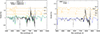 |
Fig. D.1. The SYN++ modeling of one of the spectra of SN 2020xga (left) and SN 2022xgc (right). The observed spectra (black lines) are corrected for interstellar reddening and redshift, and continuum-normalized for clarification. The best-fit model obtained using SYN++ is shown with blue and green colors, while the contribution of the single ions to the model are plotted with orange, and shifted vertically. |
Best-fit parameter values of the SYN++ modeling of the spectra of SN 2020xga and SN 2022xgc. The fit parameters are the following: the velocity at the photosphere (vphot [103 km s−1]), the photospheric temperature (Tphot [1000 K]), the optical depth of each ion (log τ [–]), the inner velocity of the line forming region (vmin [103 km s−1]), the outer velocity of the line forming region (vmax [103 km s−1]), the scale hight of the optical depth (aux [103 km s−1]), and the excitation temperature of each ion (Texc [1000 K]).
All Tables
Priors and posterior of the parameters fit with REDBACK for the generalized magnetar model.
Observations log of the imaging polarimetry observations. N.A. means Not Available.
Polarimetry results on SN 2022xgc obtained in the R-band and V-band Bessel filters. (a): Stokes parameters, and , directly obtained from the ALFOSC data frames Extraordinary and Ordinary images without applying any further corrections. (b): instrumental polarization corrected. (c): instrumental polarization corrected and polarization angle corrected. (d): instrumental polarization corrected, polarization angle corrected and bias corrected.
Best-fit parameter values of the SYN++ modeling of the spectra of SN 2020xga and SN 2022xgc. The fit parameters are the following: the velocity at the photosphere (vphot [103 km s−1]), the photospheric temperature (Tphot [1000 K]), the optical depth of each ion (log τ [–]), the inner velocity of the line forming region (vmin [103 km s−1]), the outer velocity of the line forming region (vmax [103 km s−1]), the scale hight of the optical depth (aux [103 km s−1]), and the excitation temperature of each ion (Texc [1000 K]).
All Figures
|
Fig. 1. Images of the fields of SN 2020xga (a) and SN 2022xgc (b). Panel a: Legacy Survey DR10 image of the field of SN 2020xga before explosion. A faint host galaxy at the SN position is visible, marked by the white crosshairs. Right: gri composite image of the SN near peak from Liverpool Telescope (LT). Panel b: Pan-STARRS image of the field of SN 2022xgc before explosion. The SN position is marked by the white crosshairs. Right: gri composite image of the SN near peak from the LT. All images have a size of 2 × 2 arcmin and have been combined following the algorithm in Lupton et al. (2004). |
| In the text | |
|
Fig. 2. Optical light curves of SN 2020xga (left panel) and SN 2022xgc (right panel). The magnitudes are corrected for MW extinction and K-correction. Upper limits are presented as downward-pointing triangles in a lighter shade. The epochs of the spectra are marked as thick lines at the top of the figure. The dashed line represents the estimated time of the first light. The x axis is in rest-frame days with respect to the rest-frame g-band maximum. |
| In the text | |
|
Fig. 3. Comparison of the photometric properties of SN 2020xga, SN 2022xgc, SN 2018ibb and iPTF16eh with the ZTF SLSN-I sample (Chen et al. 2023a). Top: KDE distribution of the Mg peak magnitudes for 78 ZTF SLSNe-I. Second: KDE plot of the e-folding rise time for 69 ZTF SLSNe-I. Third: e-folding decline time distribution for 54 ZTF SLSNe-I. Bottom: Rest-frame peak g − r color distribution for 39 ZTF SLSNe-I. The vertical colored lines along with the errors (shaded regions) illustrate the positions of SN 2020xga, SN 2022xgc, SN 2018ibb and iPTF16eh and the vertical black lines the median values of the ZTF sample. |
| In the text | |
|
Fig. 4. Blackbody temperatures and radii of SN 2020xga, SN 2022xgc, SN 2018ibb and iPTF16eh. Top: Temperature evolution of SN 2020xga, SN 2022xgc, SN 2018ibb and iPTF16eh derived from the blackbody fits to the photometric (circle symbols) and the spectroscopic (star symbols) data. The gray background points represent the temperature evolution of the ZTF sample (Chen et al. 2023a). Bottom: Blackbody radius evolution of SN 2020xga, SN 2022xgc, SN 2018ibb and iPTF16eh utilizing photometry and spectra in comparison with the ZTF sample (gray). The arrows indicate the epochs where the X-shooter spectra of SN 2020xga and SN 2022xgc show the second Mg II absorption system. |
| In the text | |
|
Fig. 5. Bolometric light curves of SN 2020xga and SN 2022xgc with bolometric corrections applied. The circles correspond to the derived luminosities using gro filters and the open square symbols illustrate the bolometric luminosity assuming the same bolometric correction as the nearest epochs with multiband data. The error bars represent statistical errors. |
| In the text | |
|
Fig. 6. Rest-frame g-band absolute magnitude light curves of SN 2020xga and SN 2022xgc in comparison with iPTF16eh and SN 2018ibb. The magnitudes are K-corrected and corrected for MW extinction. The x axis is in rest-frame days with respect to the g-band peak, with the exception of iPTF16eh, where the u band was utilized for estimating the peak owing to the lack of data in the rising part of the g-band light curve. |
| In the text | |
|
Fig. 7. Multiband light curves of SN 2020xga (left panel) and SN 2022xgc (right panel) with their resulting fits from REDBACK. The solid colored lines indicate the light curves from the model with the maximum likelihood, while the shaded areas depict the 90% credible interval. The x axis is in rest-frame days with respect to the rest-frame g-band maximum. |
| In the text | |
|
Fig. 8. Host galaxy absorption and emission lines in the X-shooter spectrum of SN 2020xga (panel a) −8.3 days and SN 2022xgc (panel b) +21.9 days after maximum light. The vertical lines illustrate the various redshift values of the galaxy lines. Panel a: In the spectrum of SN 2020xga,, the emission lines (dashed red lines) give a consistent redshift of z = 0.4287, whereas the strong (dashed blue line) and weak (dashed gold line) absorption lines indicate redshifts of z = 0.4283 and z = 0.4296, respectively. Panel b: The host galaxy lines (dashed gold line) of SN 2022xgc agree on a redshift of z = 0.3103. |
| In the text | |
|
Fig. 9. Spectral sequence of SN 2020xga (panel a) from −9 to +37.8 rest-frame days and SN 2022xgc (panel b) from −0.7 to +92.1 g-band rest-frame days. An offset in flux was applied for illustration purposes. The spectroscopic measurements have undergone absolute flux calibration to align with the photometric data. The spectra are corrected for MW extinction and are smoothed using a Savitzky-Golay filter. The original data are presented in lighter colors. Regions of strong atmospheric absorption are blue-shaded. |
| In the text | |
|
Fig. 10. X-shooter spectra of SN 2020xga (upper panel) at −8.3 and +37.8 days and SN 2022xgc (lower panel) at +21.9 and +92.1 days after maximum light. The spectra are corrected for MW extinction and are smoothed using a Savitzky-Golay filter. The original spectra are shown in lighter gray. The most conspicuous features are labeled. Uncertain line identifications are denoted with question marks. The ions beneath the spectrum are shown at the rest wavelength, whilst those above have been shifted to match the absorption component. The light blue regions represent the telluric absorptions. |
| In the text | |
|
Fig. 11. Fe II triplet λλ4923, 5018, 5169 region of SN 2020xga (left panel) at −8.3 and +37.8 day spectra and SN 2022xgc at +21.9, +65.5 and +92.1 days spectra. A normalization and an arbitrary offset has been applied for illustration purposes. The spectra have been smoothed using the Savitzky-Golay filter and the original data are shown in lighter colors. The absorption features that correspond to the blueshift of the Fe II lines are denoted along with the velocities. |
| In the text | |
|
Fig. 12. Fe II ejecta velocities of SN 2020xga and SN 2022xgc as measured from the X-shooter spectra as a function of time. The velocity evolution of the ZTF SLSN-I sample is shown in gray for comparison. The vertical dash-dotted line illustrates the phase of the maximum light. |
| In the text | |
|
Fig. 13. Spectral comparison of SN 2020xga and SN 2022xgc with SLSNe-I from the literature. Left: Comparison of SN 2020xga and SN 2022xgc spectra with typical well-studied SLSNe-I at similar epochs. Right: SN 2020xga and SN 2022xgc spectra in comparison with SLSNe-I that display the second narrow Mg II absorption system. All spectra are corrected for MW extinction and have been smoothed using a Savitzky-Golay filter. |
| In the text | |
|
Fig. 14. X-shooter spectra of SN 2020xga at −8.3 days (top panel) and SN 2022xgc at +21.9 days (bottom panel). The spectra show resolved, narrow absorption lines from the host ISM (marked by the vertical dashed orange lines) and a blueshifted absorption line system (marked by the vertical dashed purple lines) from a CSM shell expelled shortly before the SN explosion. |
| In the text | |
|
Fig. 15. Modeling on the Mg II doublets originating from the CSM shell (broad features) and the ISM of the host galaxy (narrow features) for SN 2020xga (top) and SN 2022xgc (bottom). The observed spectrum in the 2800 Å region is presented in gray and the best model fit is shown in red. The dashed blue line illustrates the SN continuum. For SN 2020xga we have marked the CaH [MYAMP] K lines from the MW. |
| In the text | |
|
Fig. 16. Comparison of the broad Mg II lines originating from the CSM shells for SN 2020xga, SN 2022xgc, SN 2018ibb and iPTF 16eh. The spectra are corrected for MW extinction. The vertical black lines mark the velocity of the absorption minima of the secondary Mg II lines. |
| In the text | |
|
Fig. 17. Modeling on the Mg II doublets originated from the CSM shell (broad features) and the ISM of the host galaxy (narrow features) for SN 2018ibb. The observed spectrum at the 2800 Å region is presented in gray and the best model fit in red. The dashed blue line illustrates the SN continuum. |
| In the text | |
|
Fig. 18. Spectral energy distribution of the host galaxy of SN 2020xga (black data points). The solid line displays the best-fitting model of the SED. The red squares represent the model-predicted magnitudes. The fitting parameters are shown in the upper-left corner. The abbreviation ‘n.o.f.’ stands for the number of filters. |
| In the text | |
|
Fig. D.1. The SYN++ modeling of one of the spectra of SN 2020xga (left) and SN 2022xgc (right). The observed spectra (black lines) are corrected for interstellar reddening and redshift, and continuum-normalized for clarification. The best-fit model obtained using SYN++ is shown with blue and green colors, while the contribution of the single ions to the model are plotted with orange, and shifted vertically. |
| In the text | |
Current usage metrics show cumulative count of Article Views (full-text article views including HTML views, PDF and ePub downloads, according to the available data) and Abstracts Views on Vision4Press platform.
Data correspond to usage on the plateform after 2015. The current usage metrics is available 48-96 hours after online publication and is updated daily on week days.
Initial download of the metrics may take a while.