| Issue |
A&A
Volume 689, September 2024
|
|
|---|---|---|
| Article Number | A60 | |
| Number of page(s) | 7 | |
| Section | Stellar structure and evolution | |
| DOI | https://doi.org/10.1051/0004-6361/202449919 | |
| Published online | 30 August 2024 | |
Primary and secondary source of energy in the superluminous supernova 2018ibb
1
Heidelberger Institut für Theoretische Studien, Schloss-Wolfsbrunnenweg 35, 69118 Heidelberg, Germany
2
GSI Helmholtzzentrum für Schwerionenforschung, Planckstraße 1, 64291 Darmstadt, Germany
3
National Research Center, Kurchatov Institute, pl. Kurchatova 1, Moscow 123182, Russia
4
Lebedev Physical Institute, Russian Academy of Sciences, 53 Leninsky Avenue, Moscow 119991, Russia
5
Space Research Institute (IKI), Profsoyuznaya 84/32, Moscow 117997, Russia
6
M.V. Lomonosov Moscow State University, Sternberg Astronomical Institute, 119234 Moscow, Russia
7
Astronomisches Rechen-Institut, Zentrum für Astronomie der Universität Heidelberg, Mönchhofstr. 12-14, 69120 Heidelberg, Germany
Received:
9
March
2024
Accepted:
30
May
2024
Abstract
We examined a possible pair-instability origin for the superluminous supernova 2018ibb. As the base model, we used a non-rotating stellar model with an initial mass of 250 M⊙ at about 1/15 solar metallicity. We considered three versions of the model as input for radiative transfer simulations done with the STELLA and ARTIS codes: with 25 M⊙ of 56Ni, with 34 M⊙ of 56Ni, and a chemically mixed case with 34 M⊙ of 56Ni. We present light curves and spectra in comparison to the observed data of SN 2018ibb, and conclude that the pair-instability supernova model with 34 M⊙ of 56Ni explains the broadband light curves reasonably well between −100 and 250 days around the peak. Our synthetic spectra have many similarities with the observed spectra. The luminosity excess in the light curves and the blue-flux excess in the spectra can be explained by an additional energy source, which may be an interaction of the supernova ejecta with circumstellar matter. We discuss possible mechanisms that could have caused the circumstellar matter to be ejected in the decades before the pair-instability explosion.
Key words: radiative transfer / circumstellar matter / stars: massive / supernovae: general / supernovae: individual: 2018ibb
Corresponding author; This email address is being protected from spambots. You need JavaScript enabled to view it. .
© The Authors 2024
 Open Access article, published by EDP Sciences, under the terms of the Creative Commons Attribution License (https://creativecommons.org/licenses/by/4.0), which permits unrestricted use, distribution, and reproduction in any medium, provided the original work is properly cited.
This article is published in open access under the Subscribe to Open model. This email address is being protected from spambots. You need JavaScript enabled to view it. to support open access publication.
1. Introduction
The superluminous supernova (SLSN) 2018ibb is a unique supernova (SN) event that was discovered long before its peak (Tonry et al. 2018). It was classified as hydrogen- and helium-free (i.e. a Type I SLSN) when the first spectral data were collected around its maximum (Pursiainen et al. 2018)1. The study of SN 2018ibb has benefited from an exquisite follow-up campaign and exclusively good data coverage starting from 100 days before peak magnitude, or 109 days in the Gaia G band in the observer’s frame (Schulze et al. 2024). The absolute peak magnitude of −21.5 mags and the long rise of 100 days to the peak indicate a high mass of radioactive nickel 56Ni, about 30 M⊙, and a long diffusion time, which implies a high ejecta mass. From a theoretical point of view, it is well known that stars with initial hydrogenic mass in the range 140–260 M⊙ undergo pair instability (PI) and explode as pair-instability supernovae (PISNe; Barkat et al. 1967; Rakavy & Shaviv 1967). Depending on the mass of a carbon-oxygen core formed by the PI episode, a broad range of a total radioactive 56Ni yields are produced, from 0 to up to 60 M⊙ (Heger & Woosley 2002; Takahashi et al. 2016). Therefore, the resulting SN can be either sub- or superluminous (−14 mag to −22 mag in V; Kasen et al. 2011), with broad light curves that rise to the peak over 100–150 days.
In the present study, we examined and confirm a PISN origin for SN 2018ibb2. We specifically chose SN 2018ibb because it passed a number of tests showing that no other mechanisms, such as magnetar or pure interaction, can explain its origin. For instance, SN 2018ibb was observed for more than 1000 days and does not show a signature of a different slope at late times, which would be expected for magnetar-powered SNe (Moriya et al. 2017). SN 2018 is the best PISN candidate we have today. Other Type Ic SLSNe are supposedly powered by a magnetar or interaction (Nicholl et al. 2013; Chen et al. 2015).
Details of our progenitor and explosion models and the techniques we used to model light curves and spectra are given in Section 2. In Section 3 we present synthetic observables for our models, compare them to observations, and discuss the primary and secondary sources of energy in SN 2018ibb. We summarise our study in Section 4.
2. Progenitor model and modelling of light curves and spectra
2.1. Explosion models
To explain SN 2018ibb’s high luminosity of log L ∼ 44.25 erg s − 1, about 36 M⊙ of radioactive nickel 56Ni is required assuming the nickel-powering mechanism is at play (Kozyreva et al. 2016). According to Heger & Woosley (2002), this amount of 56Ni can be produced by a PI explosion of a star with a He core of 126 M⊙, a star that was originally hydrogenic and had an initial mass of about 250 M⊙ (see Eq. (1) in Heger & Woosley 2002). Therefore, we focused our modelling on a very massive non-rotating star model, P250, with MZAMS = 250 M⊙ at a metallicity of Z = 0.001 (Z ≅ 0.07 Z⊙, where Z⊙ = 0.014; Asplund et al. 2005). Our choice of metallicity is not precisely consistent with the claimed metallicity of the host of SN 2018ibb, 0.25 Z⊙ (Schulze et al. 2024). We note, though, that the host metallicity, given with some degree of uncertainty, is an averaged metallicity based on the measurements of many HII regions, and it could not be specified for the exact SN explosion site. In any case, both the host metallicity and the stellar model metallicity are sub-solar. The stellar model P250 was evolved from the zero age main sequence (ZAMS) until the start of the PI phase using the stellar evolution code GENEC (Ekström et al. 2012; Yusof et al. 2013). The radius of the model is 2 R⊙ and the mass is 127 M⊙ prior to the PI. The star consists mainly of carbon and oxygen and has a shallow helium layer at the surface, with a total helium mass of 2.6 M⊙. The PI explosion of the original model, P250, was carried out using the FLASH code (Fryxell et al. 2000; Dubey et al. 2009; Chatzopoulos et al. 2013, 2015) while mapping the hydrodynamical and chemical profiles from GENEC into FLASH. Details about the FLASH simulations are published in Gilmer et al. (2017) and Kozyreva et al. (2017). We used the result from the FLASH simulations, namely that 33.8 M⊙ of radioactive nickel 56Ni is produced during the explosive oxygen and silicon burning. In this model the explosion energy carried by the ejecta in the form of thermal and kinetic energy is 84 foe, where 1 foe = 10 51 erg. We name this model P250Ni34. The model P250Ni34mix is the same as P250Ni34 but is chemically homogeneously mixed, that is to say, all yields are kept as in the original model P250Ni34 but all species are distributed uniformly throughout the ejecta without changing other hydrodynamical profiles, similar to in Mazzali et al. (2019). We also built another model, P250Ni25, based on model P250Ni34 but with a reduced amount of 56Ni, 24.6 M⊙ and the profile of 56Ni scaled by a factor of 2/3 to check whether the smaller yield of radioactive nickel 56Ni might power the light curve of SN 2018ibb. The missing fraction of 56Ni was replaced with silicon. A lower yield of 56Ni, 24.6 M⊙, was also obtained in one of the test FLASH simulations (M. Gilmer, private communication).
2.2. Light curve modelling
We followed the SN explosion and modelled the light curves with the one-dimensional multigroup radiation hydrodynamics code STELLA (Blinnikov et al. 1998, 2000, 2006). The description of STELLA, including details about opacities, and a comparison to other radiative transfer codes are presented in Blondin et al. (2022). We mapped the models into STELLA when the shock was close to the edge of the star (i.e. the shock breakout). In our simulations we used 100 frequency bins and a spacial grid of 231 zones.
2.3. Spectral synthesis
We used the Monte Carlo radiative transfer code ARTIS (Kromer & Sim 2009) in full non-local thermodynamic equilibrium (non-LTE) mode (Shingles et al. 2020) to compute spectral time series for the models in our study. The full non-LTE treatment includes deposition by non-thermal electrons, non-LTE ionisation balance and level populations, detailed bound-free photoionisation estimators using full packet trajectories (Eq. (44) from Lucy 2003) for all photoionisation transitions, and a non-LTE binned radiation field model for excitation transitions. Forbidden transitions are included in the dataset based on the atomic data compilation of CMFGEN3 (Hillier 1990; Hillier & Miller 1998), typically with the first five ionisation stages as detailed in Shingles et al. (2020).
As an input model for our ARTIS simulations, we used the spherically symmetric density and abundance snapshot from STELLA at 10 d after the explosion, when the ejecta are approaching homologous expansion4. We simulated the evolution of the energy flows and radiation field by propagating 5 × 10 8 Monte Carlo quanta for 150 logarithmically spaced time steps from 150 to 850 d post-explosion. The number of interactions per packet was more than 1 for a time span exceeding 600 days after the explosion. Once the Monte Carlo quanta escaped the simulation domain, they were binned in time and on a logarithmic wavelength grid spanning 1000 bins from 375 Å to 30 000 Å to obtain the spectral time series5.
In the STELLA simulations, the only source of radioactivity is radioactive nickel 56Ni, while ARTIS also includes radioactivity from 57Ni. Therefore, we artificially changed the chemical composition of the input models to consider 57Ni in the ARTIS simulations. According to the set of zero-metallicity helium PISN models from Heger & Woosley (2002), the total yield of 57Ni is about 1/50 of the 56Ni yield. Therefore, we set the quantity of 57Ni to 0.5 M⊙ in the chemical profiles mapped into ARTIS for model P250Ni25, and to and 0.7 M⊙ for P250Ni34 and P250Ni34mix. However, the 57Ni yield differs for very massive stars at non-zero metallicity, which is the case for P250 with an initial metallicity of 0.001. The 57Ni yield might be higher, by up to 10%, relative to the 56Ni yield since neutron excess is higher for higher metallicities (Umeda & Nomoto 2002; Kozyreva et al. 2014; Takahashi et al. 2018).
3. Results and discussion
In the following we first analyse the synthetic light curves in the context of the bolometric and broadband light curves of SN 2018ibb. We then present the result of the spectral synthesis and compare our models to the observed spectra of SN 2018ibb. Based on this analysis, we draw conclusion about the circumstances of the explosion of the SN 2018ibb progenitor.
3.1. Bolometric and broadband light curves
In Figure 1 we present bolometric light curves for models P250Ni25, P250Ni34, and P250Ni34mix in the rest frame6. Time t = 0 is set similar to tmax = 0 (MJD = 58455) in Schulze et al. (2024) for consistency and corresponds to the SN 2018ibb peak in the g and r bands. Our synthetic light curves are truly bolometric and correspond to an integrated flux between 1 Å and 50 000 Å. The bolometric light curve for SN 2018ibb (shown as a grey curve in Figure 1) is taken from Schulze et al. (2024). In their study, the bolometric light curve was constructed differently at different epochs. For instance, the luminosity between day 0 and day 100 was integrated over the wavelength range 1800 Å– 14 300 Å because there is a complete photometric coverage in this time window. However, the part of the bolometric light curve before the peak was based on the observed flux in the Zwicky Transient Facility g and r bands, and the correction was estimated at the first epoch with good coverage (details are provided in Section 4.2.2 of Schulze et al. 2024). In Figure 2 we present our resulting light curves in broad bands uvw2, uvm2, uvw1, u, b, g, c, v, G, r, o, i, z, J, H, and K in the rest frame and the observed broadband light curves for SN 2018ibb (Schulze et al. 2024). The rise time in the rest frame is 120 days for models P250Ni25 and P250Ni34, and 100 days for model P250Ni34mix.
 |
Fig. 1. Bolometric light curves for the models P250Ni25 (red curve, labelled ‘Ni25’), P250Ni34 (blue curve, labelled ‘Ni34’), and P250Ni34mix (cyan curve, labelled ‘Ni34mix’), and the bolometric light curve for SLSN 2018ibb (grey curve, labelled ‘2018ibb’) taken from Schulze et al. (2024). Time ‘0’ corresponds to the peak in g and r-band magnitude, similar to the tmax in Schulze et al. (2024). |
 |
Fig. 2. Broadband magnitudes for three models in the study in comparison to those for SN 2018ibb (grey circles; Schulze et al. 2024). Red, blue, and cyan curves represent the P250Ni25, P250Ni34, and P250Ni34mix models, respectively. |
There is a generally good agreement between the available data and model P250Ni34 starting from the non-detection epoch until day 250 after the peak (i.e. over 450 days). Therefore, it is clear that the primary source of energy powering the light curve of SN 2018ibb is radioactive nickel 56Ni produced in the PI explosion. However, there are some differences between the observed and synthetic light curves. Model P250Ni25 clearly underestimates the flux in many broad bands, though it agrees reasonably well with SN 2018ibb in the uvw2, uvm2, uvw1, and u bands. The uniform mixing in model P250Ni34mix helps reduce the rise time to 100 days in the rest frame. In this model, radioactive 56Ni is distributed up to the edge while being mixed, and therefore diffusing high energy photons reach the emitting front faster. Consequently, P250Ni34mix produces a perfect fit to the rising part of the SN 2018ibb bolometric light curve. However, the photons then easily escape from the ejecta, lowering the flux in the uvw2, uvm2, and uvw1 bands and weakening the suitability of model P250Ni34mix. Furthermore, the bolometric luminosity at the peak is also lower because the amount of radioactive energy contained in the inner region is reduced due to the lower mass fraction of 56Ni compared to the unmixed case, P250Ni34, although the total mass of 56Ni is the same. We note that light curves in the J and H bands systematically deviate from the observed light curves. The list of line transitions implemented in STELLA is likely not exhaustive enough to make a solid prediction for the flux in these bands, although good agreement to more sophisticated spectral synthesis codes shows that the STELLA simulations are suitable for these wavelengths when applied to SNe Ia (see Fig. 8 in Blondin et al. 2022).
Our models deviate noticeably from observations later than day 200 after the peak. There are a few episodes, which we call ‘bumps’ later in the paper, where the observed light curve clearly deviates from the modelled light curve. Another, secondary energy source likely contributes to the light curve at a later time, which we discuss below.
3.2. Spectral comparison to SN 2018ibb
In Figure 3, series of synthetic spectra are presented for the same selected epochs in the rest frame as the observed spectra (S. Schulze, private communication; we used the spectra which were corrected for galactic extinction and the host): days 94, 231, 286, and 3627. We show three theoretical sets in the plots: (1) P250Ni25 is in red, (2) P250Ni34 is in blue, and (3) P250Ni34mix is in cyan. The observed spectra (shown in grey) have been converted to the rest frame8. Each observed spectrum has been smoothed with a median filter (window size of ten data points; Pratt 2007) for demonstrative purposes. All the spectra in Figure 3 have been normalised by a different factor for each subplot, which corresponds to the maximum flux value in a given subplot. We emphasise that the synthetic light curves were computed with the STELLA code and the spectral synthesis was carried out with the ARTIS code; therefore, there is some discrepancy between the flux in the spectra at a particular epoch and the magnitude in broad bands. Nevertheless, the STELLA and ARTIS broadband light curves are consistent with each other.
 |
Fig. 3. Spectral series of synthetic spectra with observational data superimposed. Red, blue, and cyan curves represent the P250Ni25, P250Ni34, and P250Ni34mix models, respectively. The observed spectra (shown in grey) are different from those published in Schulze et al. (2024) because we plotted spectra corrected for galactic extinction and the host (S. Schulze, private communication). Days are since the g and r maximum in the rest frame. Spectra are calibrated to the maximum flux values in each subplot. A rise time of 120 days is assumed for the P250Ni34 and P250Ni25 models, and 100 days for P250Ni34mix. |
There is an overall good (albeit not exact) agreement between the observed and synthetic spectra, particularly for our best fitting model P250Ni34, in redder wavelengths. At day 231 and later, there is a pronounced flux excess in blue wavelengths. The differences between the observed spectra and the synthetic spectra are mainly seen below 5500 Å. The maximum in the residual ‘spectra’ is located at a wavelength of 4000 Å and does not move noticeably between day 231 and day 362. The decreasing residual flux is likely explained by the decreasing size of the emitting region. This might be consistent with the findings by Schulze et al. (2024), who claim that there is an occultation of circumstellar matter (CSM) by the SN ejecta in SN 2018ibb, based on an analysis of the late time evolution of the [O II] λλ 7318, 7330 lines.
The largest contribution to the flux comes from [Fe II] emission, but there are prominent lines from other ions. Below we mention a couple of prominent lines seen in the synthetic and observed spectra:
-
[Ca II] λ 3969 is seen in modelled spectra at all epochs; however, it does not reproduce the observed line, partly because of additional flux in the blue wavelengths.
-
[O III] λ 5007, which is formed in the low-density environment and indicates an interaction, is not reproduced in the model spectra due to the low ionisation state of O (mostly neutral).
-
[O I] λλ 6300, 6364 is present in both the synthetic and observed spectra at day 231 and later, although the shape of the synthetic line differs from the observed one.
-
A blend of [O II] λλ 7318, 7330 and [Ca II] λλ 7291, 7323 is seen in SN 2018ibb and is reproduced by our models to some extent. At an earlier epoch (day 94) the unmixed models overestimate flux in this blend, while at later epochs (later than 2231 days) the models still display this blend, but the flux is underestimated. In the last shown epoch, day 362, the mixed model is able to reproduce the line quite well, which means that there should be some oxygen with a low velocity and low electron density.
-
The synthetic line [O I] λ 7773 can be considered to match the observed line throughout the entire evolution, though with a slightly different strength and shape.
-
[Ca II] λλ 8544, 8664 is present in both the synthetic spectra and observations of SN 2018ibb.
We also note that spectra on day 600 are not yet nebular, since there are quite a few interactions between packets.
Presumably, the spectra of SN 2018ibb are a superposition of two types of spectra or two mechanisms, one of which is flux from the pure PISN explosion. In other words, there should be an additional source of energy input on top of the flux coming from the PISN itself: the PISN models explain the light curves of SN 2018ibb considerably well and partially explain the spectra, meaning that PISN radiation is a major contributor to the flux from SN 2018ibb. The residual flux can be explained by an interaction of SN ejecta with the surrounding CSM, which is consistent with the conclusions from Schulze et al. (2024).
3.3. The secondary energy source in SN 2018ibb
SN 2018ibb undergoes re-brightening, including variations, around day 50 after the maximum in the uvw2, uvm2, uvw1, and u bands and after day 200 in redder bands, which is not predicted by our models. A number of SLSNe also display bumps in their light curves (i.e. they deviate from the linear decline; Hosseinzadeh et al. 2022; Chen et al. 2023). Re-brightening or bumps might be caused when the ejecta encounter clumps (see e.g. Dessart & Audit 2019) or shells located at some distance from the progenitor (Aamer et al. 2024). Schulze et al. (2024) reveal several signatures of CSM interaction based on their analysis of spectra: (1) an Mg II absorption line system moving at a significantly lower velocity than the SN ejecta; (2) the simultaneous emergence of [O II] and [O III] emission at 30 rest-frame days after maximum; and (3) detection of the [O III] line 1000 days after peak in the rest frame.
We used the bolometric light curve to analyse the luminosity excess between 42 days before the peak and 600 days after the peak. Based on the timing of the maximum (i.e. the rise time), at 120 days since the explosion for P250Ni34, the distance to CSM or a shell can be estimated as RCSM = tmax × v, where tmax = 120 days, and v = 10 10 cm s − 1 is the velocity of the outer ejecta; according to this calculation, the distance to the shell is about 10 17 cm. Assuming a CSM velocity of about 3000 km s − 1, as derived in Schulze et al. (2024), the matter had to be expelled by the progenitor roughly 11 yr before the PI explosion. The luminosity excess integrated over the duration of bumps corresponds to radiated energy of 8.1 × 10 50 erg. If the ejecta collide with a shell or a blob, the outermost part of the ejecta interacts with the blob, and not the entire ejecta. Assuming that the kinetic energy of the outer ejecta is converted into radiated energy with an efficiency of, for example, 90% (i.e. Erad = Ekin, out, ej × 90%), the required mass of the ejecta interacting with the shell is about 0.02 M⊙. Following the simplified approach from Moriya et al. (2018), the mass of the CSM equals 0.4 M⊙. The detailed modelling of the ejecta interacting with the CSM and predictions of observational features, such as properly calculated light curves and spectra, are beyond of the scope of the current paper and require a separate thorough study.
If we consider the interaction as a primary source, then the resulting light curve will not last very long, and a large amount of radioactive nickel will be needed to explain the late-time luminosity. For instance, Tolstov et al. (2017) show that the light curve of PTF12dam requires 43 M⊙ of SN ejecta interacting with 37 M⊙ of CSM and 6 M⊙ of radioactive nickel. In their simulations the ‘interaction’ part of the light curve lasts about 200 days and can explain the main maximum of PTF12dam, that is to say, the interaction is presumably the primary powering mechanism. However, PTF12dam requires a secondary energy source to explain the later decline of the light curve. Nevertheless, we note that the light curve of PTF12dam is significantly narrower than that of SN 2018ibb (see Fig. 31 of Schulze et al. 2024), and this scenario, specifically the interaction mechanism, is not relevant for SN 2018ibb.
The next underlying question is which process is behind the non-steady ejection of a stellar matter 11 yr before an explosion. In the case of massive and very massive stars, it corresponds to core carbon burning. Single stellar evolution models, like our P250 model, experience massive wind mass-loss during hydrogen core burning, thousands of years before their PI explosion (Yusof et al. 2013). Therefore, this matter, being hydrogen-rich, dissolves by the time of the explosion. Moreover, SN 2018ibb is hydrogen- and helium-free, which means that the ejecta and CSM do not contain these elements. Moriya & Langer (2015) suggest that pulsation-driven mass loss in metal-free, very massive stars may produce a dense CSM; however, their findings are mostly applicable to Type IIn SLSNe. We note that the amount of CSM required to explain the luminosity excess is very low, about 0.4 M⊙ in total, as roughly estimated above. This amount of matter could not originate from previous binary interactions, such as a stellar merger or a common envelope ejection, both of which would lead to a loss of about 10% of the total mass of a system (i.e. a much greater mass loss; LBV-like (LBV – Luminous blue variable) eruptions caused by envelope inflation cannot be a mechanism for the production of H-free ejecta in our case (see e.g. Sanyal et al. 2015). Moreover, a merger or a common envelope phase only years before the SN explosion would require extreme fine-tuning (Chevalier 2012). Nevertheless, those very massive stars spend their late stages of evolution as He stars. In the case of the P250 model, the final configuration is mainly a pure CO core with a tenuous layer of helium, meaning that nuclear burning takes place near the surface. Any nuclear burning, waves excited by nuclear burning, or helium shell burning (see Figure 1 in Kozyreva et al. 2017) could cause the ejection of a negligible amount hydrogen-free material in the last years before the explosion (e.g. Quataert & Shiode 2012; Quataert et al. 2016, and other studies).
3.4. ARTIS versus SEDONA and SUMO
Spectral synthesis simulations for PISN models were also performed with SEDONA (Kasen et al. 2011), CMFGEN (Dessart et al. 2013), and SUMO (Jerkstrand et al. 2016). It is difficult to make a direct comparison because the mapped PISN models are different. The two highest-mass PISN models in Dessart et al. (2013) are: a 100 M⊙ He star with 5 M⊙ of 56Ni, which is too low to compare to our high-mass model P250, and a relatively extended (146 R⊙) H-rich blue supergiant model with a total mass of 210 M⊙ and with 21 M⊙ of 56Ni, which cannot be used for comparison to our compact H-free P250 model.
The input model for the SEDONA and SUMO simulations was a 130 M⊙ helium-core model, He130 (Heger & Woosley 2002). Our input model was a hydrogenic star with an initial mass of 250 M⊙ that loses all hydrogen during its earlier evolution and forms a He core of 127 M⊙, making it similar to the He130 model. Differences include the total amount of radioactive nickel 56Ni produced during the PI explosion and the amount of energy: 34 M⊙ and 40 M⊙, and 82 foe and 87 foe in our P250 model and their He130 model, respectively. Therefore, we chose the He130 model used in the SEDONA and SUMO simulations and our model P250Ni34 to validate whether the spectra from model P250Ni34 are in qualitative agreement with published PISNe synthetic spectra.
In Figure 4 we show spectra of the He130 model computed with SEDONA and SUMO together with the spectrum for our model P250Ni34. The SUMO and our ARTIS spectra at 250 day after the peak have many common features. Among them are [Si I] λ 4131, [Ca II] λλ 7291, 7323, [O I] λ 7773, and many Fe II lines. The flux in the ARTIS spectra being higher than in the SUMO spectra can be explained by the fact that the ejecta at this epoch are still not fully transparent and therefore do not produce a pure nebular emission. The agreement between the SEDONA spectra and our ARTIS spectra is poor because SEDONA simulations are performed assuming a LTE approximation for ionisation states and level populations, while our ARTIS simulations were carried out in full non-LTE. A direct comparison of ARTIS simulations in application to SN Ia spectra was done in separate studies, for example Shingles et al. (2020) and Blondin et al. (2022).
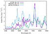 |
Fig. 4. SUMO and SEDONA spectra for the He130 model on day 400, and the ARTIS spectrum on day 371. |
4. Conclusions
We have examined the possibility of a PISN origin for the SLSN 2018ibb. We used the stellar evolution model of a very massive star with an initial ZAMS mass of 250 M⊙ at metallicity Z = 0.001 (Z ≅ 0.07 Z⊙, where Z⊙ = 0.014). The calculations were carried out using (1) the GENEC code to compute the stellar evolution, (2) the FLASH code to follow the dynamical phase of explosive oxygen burning, collapse, and PI explosion (Gilmer et al. 2017; Kozyreva et al. 2017), and (3) the radiative-transfer codes STELLA and ARTIS to follow up on the hydrodynamical evolution of the ejecta and radiation field and to calculate observational properties, such as light curves and spectra. We find that the PI explosion of such a very massive star with 34 M⊙ of radioactive nickel 56Ni provides a good match to the bolometric and broadband light curves of SN 2018ibb over a long time interval (i.e. from the explosion until 250 days after the peak). The synthetic spectra match the observed spectra to a large extent, including the appearance of many lines and the colour evolution. We emphasise that the best-fitting model is physically consistent from the dawn of the progenitor life until its explosion becomes invisible, and the good match is exceptional given that our model has not been tuned to fit either the light curves or the spectra.
Nevertheless, our PISN models suffer from a flux deficit in the blue wavelengths between 3000 Å and 5000 Å, while the observed spectra clearly show a significant flux. This indicates that there is a secondary source of energy powering the radiation field of SN 2018ibb. Among the possibilities, we suggest an interaction of the PISN ejecta with CSM, which may produce the additional blue flux missing in the PISN model. Our analysis of the light curve shows that a series of mass eruptions happened before the final PI explosion. The amount of matter required to explain the flux excess is about 0.4 M⊙, which might originate from some activity during the latest evolution phases of the star caused by nuclear instabilities in the outermost atmosphere. We estimate that this material is located at a distance of 0.2 pc from the progenitor and was ejected by a progenitor decades prior to the PI explosion. The nature of the pre-explosion ejection might be instabilities caused by nuclear burning happening in the outer layers of the progenitor.
Data availability
The data computed and analysed for the current study are available via the link https://zenodo.org/doi/10.5281/zenodo.10473678.
The first classification was done by Fremling et al. (2018); however, they misclassified SN 2018ibb as a Type Ia SN.
Another study exploring different PISN models in application to SN 2018ibb was submitted during the reviewing stage of the present paper, Nagele et al. (2024). Based on the derived photospheric parameters, the authors rule out a PISN origin for SN 2018ibb.
Available at http://kookaburra.phyast.pitt.edu/hillier/web/CMFGEN.htm
Note, though, that the Ni-bubble effect develops over a timescale of 100 days; however, there is no significant contribution to the observables. See the discussion in Kozyreva et al. (2017).
For the Ni34 model, the computational cost was 367 hours on 960 cores (352 k core hours). For Ni25, the cost was 422 hours on 960 cores (405 k core hours).
We note that this light curve for model P250Ni34 differs from those published in Kozyreva et al. (2017) and Schulze et al. (2024) because we fixed a numerical issue caused by the high velocity of the ejecta.
The entire set of ARTIS spectra between day 150 and day 850 after the explosion is available via https://zenodo.org/doi/10.5281/zenodo.10473678.
 , where z = 0.166 is the redshift and D = 882.6 Mpc is a distance to SN 2018ibb.
Acknowledgments
We thank Steve Schulze, Pavel Abolmasov, Marat Potashov, Elena Sorokina, and Sergei Blinnikov for helpful discussions. AK acknowledges support by Alexander von Humboldt Stiftung. LJS acknowledges support by the European Research Council (ERC) under the European Union’s Horizon 2020 research and innovation program (ERC Advanced Grant KILONOVA No. 885281). LJS acknowledges support by Deutsche Forschungsgemeinschaft (DFG, German Research Foundation) – Project-ID 279384907 – SFB 1245 and MA 4248/3-1. PB is sponsored by grant RSF 23-12-00220 in his work on the STELLA code development. This project began before February 2022.
References
- Aamer, A., Nicholl, M., Jerkstrand, A., et al. 2024, MNRAS, 527, 11970 [Google Scholar]
- Asplund, M., Grevesse, N., & Sauval, A. J. 2005, ASP Conf. Ser., 336, 25 [Google Scholar]
- Barkat, Z., Rakavy, G., & Sack, N. 1967, Phys. Rev. Lett., 18, 379 [Google Scholar]
- Blinnikov, S. I., Eastman, R., Bartunov, O. S., Popolitov, V. A., & Woosley, S. E. 1998, ApJ, 496, 454 [Google Scholar]
- Blinnikov, S., Lundqvist, P., Bartunov, O., Nomoto, K., & Iwamoto, K. 2000, ApJ, 532, 1132 [NASA ADS] [CrossRef] [Google Scholar]
- Blinnikov, S. I., Röpke, F. K., Sorokina, E. I., et al. 2006, A&A, 453, 229 [NASA ADS] [CrossRef] [EDP Sciences] [Google Scholar]
- Blondin, S., Blinnikov, S., Callan, F. P., et al. 2022, A&A, 668, A163 [NASA ADS] [CrossRef] [EDP Sciences] [Google Scholar]
- Chatzopoulos, E., van Rossum, D. R., Craig, W. J., et al. 2015, ApJ, 799, 18 [NASA ADS] [CrossRef] [Google Scholar]
- Chatzopoulos, E., Wheeler, J. C., & Couch, S. M. 2013, ApJ, 776, 129 [NASA ADS] [CrossRef] [Google Scholar]
- Chen, T. W., Smartt, S. J., Jerkstrand, A., et al. 2015, MNRAS, 452, 1567 [NASA ADS] [CrossRef] [Google Scholar]
- Chen, Z. H., Yan, L., Kangas, T., et al. 2023, ApJ, 943, 42 [NASA ADS] [CrossRef] [Google Scholar]
- Chevalier, R. A. 2012, ApJ, 752, L2 [NASA ADS] [CrossRef] [Google Scholar]
- Dessart, L., & Audit, E. 2019, A&A, 629, A17 [NASA ADS] [CrossRef] [EDP Sciences] [Google Scholar]
- Dessart, L., Waldman, R., Livne, E., Hillier, D. J., & Blondin, S. 2013, MNRAS, 428, 3227 [NASA ADS] [CrossRef] [Google Scholar]
- Dubey, A., Reid, L. B., Weide, K., et al. 2009, ArXiv e-prints [arXiv:0903.4875] [Google Scholar]
- Ekström, S., Georgy, C., Eggenberger, P., et al. 2012, A&A, 537, A146 [Google Scholar]
- Fremling, C., Dugas, A., & Sharma, Y. 2018, Transient Name Server Classif. Rep., 2018-1877, 1 [Google Scholar]
- Fryxell, B., Olson, K., Ricker, P., et al. 2000, ApJS, 131, 273 [Google Scholar]
- Gilmer, M. S., Kozyreva, A., Hirschi, R., Fröhlich, C., & Yusof, N. 2017, ApJ, 846, 100 [NASA ADS] [CrossRef] [Google Scholar]
- Heger, A., & Woosley, S. E. 2002, ApJ, 567, 532 [Google Scholar]
- Hillier, D. J. 1990, A&A, 231, 116 [NASA ADS] [Google Scholar]
- Hillier, D. J., & Miller, D. L. 1998, ApJ, 496, 407 [NASA ADS] [CrossRef] [Google Scholar]
- Hosseinzadeh, G., Berger, E., Metzger, B. D., et al. 2022, ApJ, 933, 14 [NASA ADS] [CrossRef] [Google Scholar]
- Jerkstrand, A., Smartt, S. J., & Heger, A. 2016, MNRAS, 455, 3207 [NASA ADS] [CrossRef] [Google Scholar]
- Kasen, D., Woosley, S. E., & Heger, A. 2011, ApJ, 734, 102 [NASA ADS] [CrossRef] [Google Scholar]
- Kozyreva, A., Gilmer, M., Hirschi, R., et al. 2017, MNRAS, 464, 2854 [NASA ADS] [CrossRef] [Google Scholar]
- Kozyreva, A., Hirschi, R., Blinnikov, S., & den Hartogh, J. 2016, MNRAS, 459, L21 [NASA ADS] [CrossRef] [Google Scholar]
- Kozyreva, A., Yoon, S.-C., & Langer, N. 2014, A&A, 566, A146 [NASA ADS] [CrossRef] [EDP Sciences] [Google Scholar]
- Kromer, M., & Sim, S. A. 2009, MNRAS, 398, 1809 [Google Scholar]
- Lucy, L. B. 2003, A&A, 403, 261 [NASA ADS] [CrossRef] [EDP Sciences] [Google Scholar]
- Mazzali, P. A., Moriya, T. J., Tanaka, M., & Woosley, S. E. 2019, MNRAS, 484, 3451 [NASA ADS] [CrossRef] [Google Scholar]
- Moriya, T. J., & Langer, N. 2015, A&A, 573, A18 [NASA ADS] [CrossRef] [EDP Sciences] [Google Scholar]
- Moriya, T. J., Chen, T.-W., & Langer, N. 2017, ApJ, 835, 177 [NASA ADS] [CrossRef] [Google Scholar]
- Moriya, T. J., Sorokina, E. I., & Chevalier, R. A. 2018, Space Sci. Rev., 214, 59 [Google Scholar]
- Nagele, C., Umeda, H., & Maeda, K. 2024, ApJ, submitted, [arXiv:2404.16570] [Google Scholar]
- Nicholl, M., Smartt, S. J., Jerkstrand, A., et al. 2013, Nature, 502, 346 [NASA ADS] [CrossRef] [Google Scholar]
- Pratt, W. K. 2007, Digital Image Processing: PIKS Scientific Inside (John Wiley& Sons, Inc.), 738 [Google Scholar]
- Pursiainen, M., Castro-Segura, N., Smith, M., & Yaron, O. 2018, Transient Name Server Classif. Rep., 2018-2184, 1 [Google Scholar]
- Quataert, E., & Shiode, J. 2012, MNRAS, 423, L92 [NASA ADS] [CrossRef] [Google Scholar]
- Quataert, E., Fernández, R., Kasen, D., Klion, H., & Paxton, B. 2016, MNRAS, 458, 1214 [NASA ADS] [CrossRef] [Google Scholar]
- Rakavy, G., & Shaviv, G. 1967, ApJ, 148, 803 [Google Scholar]
- Sanyal, D., Grassitelli, L., Langer, N., & Bestenlehner, J. M. 2015, A&A, 580, A20 [NASA ADS] [CrossRef] [EDP Sciences] [Google Scholar]
- Schulze, S., Fransson, C., Kozyreva, A., et al. 2024, A&A, 683, A223 [NASA ADS] [CrossRef] [EDP Sciences] [Google Scholar]
- Shingles, L. J., Sim, S. A., Kromer, M., et al. 2020, MNRAS, 492, 2029 [NASA ADS] [CrossRef] [Google Scholar]
- Takahashi, K., Yoshida, T., Umeda, H., Sumiyoshi, K., & Yamada, S. 2016, MNRAS, 456, 1320 [NASA ADS] [CrossRef] [Google Scholar]
- Takahashi, K., Yoshida, T., & Umeda, H. 2018, ApJ, 857, 111 [NASA ADS] [CrossRef] [Google Scholar]
- Tolstov, A., Nomoto, K., Blinnikov, S., et al. 2017, ApJ, 835, 266 [NASA ADS] [CrossRef] [Google Scholar]
- Tonry, J., Denneau, L., Heinze, A., et al. 2018, Transient Name Server Discov. Rep., 2018-1722, 1 [Google Scholar]
- Umeda, H., & Nomoto, K. 2002, ApJ, 565, 385 [Google Scholar]
- Yusof, N., Hirschi, R., Meynet, G., et al. 2013, MNRAS, 433, 1114 [NASA ADS] [CrossRef] [Google Scholar]
All Figures
|
Fig. 1. Bolometric light curves for the models P250Ni25 (red curve, labelled ‘Ni25’), P250Ni34 (blue curve, labelled ‘Ni34’), and P250Ni34mix (cyan curve, labelled ‘Ni34mix’), and the bolometric light curve for SLSN 2018ibb (grey curve, labelled ‘2018ibb’) taken from Schulze et al. (2024). Time ‘0’ corresponds to the peak in g and r-band magnitude, similar to the tmax in Schulze et al. (2024). |
| In the text | |
|
Fig. 2. Broadband magnitudes for three models in the study in comparison to those for SN 2018ibb (grey circles; Schulze et al. 2024). Red, blue, and cyan curves represent the P250Ni25, P250Ni34, and P250Ni34mix models, respectively. |
| In the text | |
|
Fig. 3. Spectral series of synthetic spectra with observational data superimposed. Red, blue, and cyan curves represent the P250Ni25, P250Ni34, and P250Ni34mix models, respectively. The observed spectra (shown in grey) are different from those published in Schulze et al. (2024) because we plotted spectra corrected for galactic extinction and the host (S. Schulze, private communication). Days are since the g and r maximum in the rest frame. Spectra are calibrated to the maximum flux values in each subplot. A rise time of 120 days is assumed for the P250Ni34 and P250Ni25 models, and 100 days for P250Ni34mix. |
| In the text | |
|
Fig. 4. SUMO and SEDONA spectra for the He130 model on day 400, and the ARTIS spectrum on day 371. |
| In the text | |
Current usage metrics show cumulative count of Article Views (full-text article views including HTML views, PDF and ePub downloads, according to the available data) and Abstracts Views on Vision4Press platform.
Data correspond to usage on the plateform after 2015. The current usage metrics is available 48-96 hours after online publication and is updated daily on week days.
Initial download of the metrics may take a while.