| Issue |
A&A
Volume 670, February 2023
|
|
|---|---|---|
| Article Number | A7 | |
| Number of page(s) | 21 | |
| Section | Stellar structure and evolution | |
| DOI | https://doi.org/10.1051/0004-6361/202244086 | |
| Published online | 27 January 2023 | |
SN 2020qlb: A hydrogen-poor superluminous supernova with well-characterized light curve undulations
1
The Oskar Klein Centre, Department of Astronomy, Stockholm University, AlbaNova, 106 91 Stockholm, Sweden
e-mail: stuartlwest@icloud.com
2
The Oskar Klein Centre, Department of Physics, KTH Royal Institute of Technology, AlbaNova, 106 91 Stockholm, Sweden
3
The Oskar Klein Centre, Department of Physics, Stockholm University, AlbaNova, 106 91 Stockholm, Sweden
4
Benoziyo Center for Astrophysics, The Weizmann Institute of Science, Rehovot 76100, Israel
5
Astrophysics Research Institute, Liverpool John Moores University, Liverpool Science Park, 146 Brownlow Hill, Liverpool L35RF, UK
6
The Caltech Optical Observatories, California Institute of Technology, Pasadena, CA 91125, USA
7
Physics Department and Tsinghua Center for Astrophysics (THCA), Tsingua University, Beijing 100084, PR China
8
Department of Astronomy and Astrophysics, University of California, Santa Cruz, CA 95064, USA
9
Division of Physics, Mathematics, and Astronomy, California Institute of Technology, Pasadena, CA 91125, USA
10
Department of Astronomy, University of California, Berkeley, CA 94720, USA
11
Lawrence Berkeley National Laboratory, 1 Cyclotron Rd., Berkeley, CA 94720, USA
12
IPAC, California Institute of Technology, 1200 E. California Blvd, Pasadena, CA 91125, USA
Received:
23
May
2022
Accepted:
28
November
2022
Context. SN 2020qlb (ZTF20abobpcb) is a hydrogen-poor superluminous supernova (SLSN-I) that is among the most luminous (maximum Mg = −22.25 mag) and that has one of the longest rise times (77 days from explosion to maximum). We estimate the total radiated energy to be > 2.1 × 1051 erg. SN 2020qlb has a well-sampled light curve that exhibits clear near and post peak undulations, a phenomenon seen in other SLSNe, whose physical origin is still unknown.
Aims. We discuss the potential power source of this immense explosion as well as the mechanisms behind its observed light curve undulations.
Methods. We analyze photospheric spectra and compare them to other SLSNe-I. We constructed the bolometric light curve using photometry from a large data set of observations from the Zwicky Transient Facility (ZTF), Liverpool Telescope (LT), and Neil Gehrels Swift Observatory and compare it with radioactive, circumstellar interaction and magnetar models. Model residuals and light curve polynomial fit residuals are analyzed to estimate the undulation timescale and amplitude. We also determine host galaxy properties based on imaging and spectroscopy data, including a detection of the [O III]λ4363, auroral line, allowing for a direct metallicity measurement.
Results. We rule out the Arnett 56Ni decay model for SN 2020qlb’s light curve due to unphysical parameter results. Our most favored power source is the magnetic dipole spin-down energy deposition of a magnetar. Two to three near peak oscillations, intriguingly similar to those of SN 2015bn, were found in the magnetar model residuals with a timescale of 32 ± 6 days and an amplitude of 6% of peak luminosity. We rule out centrally located undulation sources due to timescale considerations; and we favor the result of ejecta interactions with circumstellar material (CSM) density fluctuations as the source of the undulations.
Key words: supernovae: general / supernovae: individual: SN 2020qlb
© The Authors 2023
 Open Access article, published by EDP Sciences, under the terms of the Creative Commons Attribution License (https://creativecommons.org/licenses/by/4.0), which permits unrestricted use, distribution, and reproduction in any medium, provided the original work is properly cited.
This article is published in open access under the Subscribe-to-Open model. Subscribe to A&A to support open access publication.
1. Introduction
The most luminous of all supernovae (SNe) are the superluminous SNe (SLSNe). Initial findings of these remarkable SNe were first made in the late 1990s but were largely explained away as scaled up versions of known SNe or as SNe Type IIn (Howell et al. 2017). Richardson et al. (2002) identified a population of rare and overluminous events. Discoveries of relatively nearby superluminous events by, for example, Quimby et al. (2007), Smith et al. (2007), Gal-Yam et al. (2009), and others marked the beginning of intensive study. Gal-Yam (2012) reviewed SLSNe and argued to divide them into subcategories, for example Type II (H-rich) and Type I (H-poor). Gal-Yam (2019) pointed out that, based on De Cia et al. (2018) and Quimby et al. (2018), H-poor SNe with peak luminosities brighter than Mg = −19.8 mag are spectroscopically similar, wherein the most important connecting features are the O II absorption lines. Further details are discussed in recent review articles (Howell et al. 2017; Gal-Yam 2019; Chen 2021; Nicholl 2021).
In general, SLSNe light curves cannot be explained by hydrogen (H) recombination or the decay of typical amounts of 56Ni, which power the majority of normal SN light curves, thereby suggesting the use of more exotic mechanisms. One such possibility is the pair-instability SN mechanism (Heger & Woosley 2002) wherein high energy photons could interact with core nucleons to form positron and electron pairs initiating a core-collapse SN explosion and creating the required large amounts of 56Ni to power the SLSN light curves. A second hypothetical light curve power source is the interaction of the SN ejecta with a circumstellar medium (CSM; e.g. Chatzopoulos et al. 2012; Sorokina et al. 2016; Wheeler et al. 2017). A third power source, the spin-down of a millisecond magnetar, (Kasen & Bildsten 2010; Woosley 2010) has emerged as a model that can fit the general shape of SLSN-I light curves (Inserra et al. 2013; Nicholl et al. 2013, 2017).
While the magnetar model has proven successful in reproducing the overall timescales and energetics of SLSNe-I, a significant number of objects also show light curve undulations that are not easily explainable in a simple magnetar spin-down scenario (e.g., Hosseinzadeh et al. 2022). The systematic monitoring and regular cadence of surveys such as the Zwicky Transient Facility (ZTF; Graham et al. 2019; Bellm et al. 2019; Masci et al. 2019) has demonstrated that such undulations are quite common, and are present in as much as 34 − 62% of SLSNe-I (Chen et al. 2022a). Similarly, Hosseinzadeh et al. (2022) found that 44 − 76% of SLSNe-I could not be explained by only a smooth magnetar model. The physical mechanism responsible for these undulations or “bumps” in the light curves is still an open question – while simple arguments based on diffusion timescales as well as bump appearance and duration times can place some constraints on them, detailed studies of such light curve undulations in multiple filters are currently lacking.
Here, we present SN 2020qlb (ZTF20abobpcb), a luminous and slow rising SLSN-I with prominent near and post peak light curve undulations. Its well-sampled light curve coverage from ZTF, the Liverpool Telescope (LT), and Swift enables us to analyze both its primary power source and the nature of the light curve undulations in detail.
This paper is organized as follows. In Sect. 2 we present the available photometric and spectroscopic data. In Sects. 3 and 4, we analyze light curve and spectral properties. In Sect. 5 we use blackbody fits to estimate the photospheric temperature and radius evolutions. In Sects. 6 and 7, we discuss the construction of the bolometric light curve and its fit with two relevant power source models. In Sect. 8 we analyze the model residuals to characterize the apparent light curve undulations. We discuss the host galaxy properties in Sect. 9. In Sect. 10 we discuss the results relative to current understandings and in Sect. 11 we conclude by summarizing our findings. We assume a flat Λ cold dark matter (ΛCDM) cosmology with H0 = 70 km s−1 Mpc−1, ΩM = 0.27, and ΩΛ = 0.73 (Komatsu et al. 2011). All magnitudes herein are in the AB system (Oke & Gunn 1983). UT dates are used throughout.
2. Observations
SN 2020qlb was discovered by the ZTF as ZTF20abobpcb on July 23, 2020 at position (J2000) right ascension (RA) 19h07m49.60s and declination (Dec) +62°57′49.52″. Figure 1 shows a pre-explosion image1 as well as an image of the supernova taken on the rise.
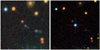 |
Fig. 1. Left: pre-SN image retrieved from the Dark Energy Camera Legacy Surveys (DR9). Right: image of SN 2020qlb taken on August 9, 2020 (61 rest frame days before peak) with the Liverpool Telescope in ugriz frames and stacked (Lupton et al. 2004) around the SN location. Each image is 45 by 45 arcsec. |
A large amount of photometric and spectroscopic data was collected for SN 2020qlb. This includes 11 spectra and 563 photometric observations, in 14 different filters, with coverage even during the SN’s solar conjunction. In this section, we describe the data collection and reduction. The explosion date is estimated in Sect. 3.1 to be MJD 59050.69 ± 0.28.
2.1. Photometry
2.1.1. ZTF photometry
The ZTF survey camera (Dekany et al. 2020) is mounted on the Palomar Observatory Schmidt 48 inch Samuel Oschin telescope which scans the night sky in search of SNe and other interesting transients. On clear nights since 2018 it has been scanning more than 2750 square degrees per hour down to 20.5 mag in the g and r filters, and less frequently in i. Data-processing pipelines, alert systems and data archival, access and analysis are performed at Infrared Processing and Analysis Center (IPAC; Masci et al. 2019), including image subtraction using the algorithm of Zackay et al. (2016). “Forced” point spread function (PSF) photometry is used to gather SN flux measurements in archived ZTF images, even from epochs prior to the transient’s initial detection. Yao et al. (2019) describe the “forced photometry” method and show that it is able to recover detections missed by the real-time pipeline as well as provide deeper predetection upper limits.
We performed the ZTF Forced PSF-fit Photometry service data reduction procedure (ver. 2.2)2 for each of the ZTF filter data sets wherein the baseline correction, the photometric uncertainty validation and the differential-photometry light curve generation were done accordingly to create observer frame light curves. There were 33 ZTFg, 34 ZTFr but zero ZTFi pre-SN baseline values identified in the data set for SN 2020qlb. We therefore estimated the baseline for the ZTFi filter so that its resulting apparent magnitudes agreed with the LT-i filter measurements taken at overlapping phases. Finally, we excluded the 23 ZTF g-band measurements where the subtracted reference values were constructed from measurements taken during the supernova rise. All photometry is listed in Table 1.
SN 2020qlb photometric observations.
We computed the absolute magnitude as

where μ is the distance modulus (=39.40 for z = 0.1583), Kcorr is the K-correction between the filter bandpass in the observer frame and the filter bandpass in the rest frame, AMW is the extinction from the Milky Way and Ahost is the extinction from the host galaxy.
The K-correction as described by Hogg et al. (2002) has two contributions: the first corrects for the redshift as

and the second corrects for the overall shape of the spectrum. We use only this first term of the K-correction; in practice, this means that all absolute magnitudes reported are at a bluer effective wavelength by a factor of (1 + z) compared to the rest wavelength of the filter. We check the impact of this, for example by comparing peak absolute magnitudes by explicitly calculating the full K-correction from a spectrum taken near peak light using the SNAKE code (Inserra et al. 2018). The result in g-band is still Kg = −0.16 ± 0.01 mag, so the peak g-band magnitude reported can be considered rest-frame.
We used the Fitzpatrick (1999) extinction model to correct for the MW dust extinction based on the parameters RV = 3.1 and E(B − V)=0.053 mag. In principle, we should also consider the possible extinction from the host galaxy. In the case of SN 2020qlb, the host is a faint, blue dwarf galaxy, similar to typical SLSN-I host galaxies (Fig. 1; Sect. 9; Lunnan et al. 2014; Perley et al. 2016). The Balmer line ratios in the host galaxy spectrum (Sect. 9) indicate some host galaxy extinction (E(B − V)host = 0.10 ± 0.05 mag). However, since we cannot know whether the extinction of this H II region is typical of the supernova site, we conservatively assume zero host galaxy extinction for the majority of the calculations in this paper. Where relevant, we point out how the results would change if host galaxy extinction was included.
2.1.2. Swift UVOT photometry
We used the UV/Optical Telescope (UVOT; Roming et al. 2005) on the Neil Gehrels (Swift) Observatory. Measurements from six different filters, ranging from the ultraviolet (UV) to visible wavelengths, were retrieved from the NASA Swift Data Archive3 and processed using UVOT data analysis software HEASoft version 6.194. Source counts were then extracted from the images using a radius of 3 arcsec, while the background was estimated using a radius of 48 arcsec around the SN position. We then used the Swift tool UVOTSOURCE to obtain the count rates from the images before converting them to magnitudes using the UVOT photometric zero points (Breeveld et al. 2011) and the September 2020 calibration files.
During 22 epochs, ranging between 26 and 143 days post explosion, all six filters were used separately to measure SN 2020qlb’s apparent AB magnitudes and their standard deviation of measurement error. Additional data are available where fewer than six filters were successfully utilized. We put all of the UVOT data into the rest frame using the procedure outlined in Sect. 2.1.1. The observed photometry is listed in Table 1, and we plot the resulting rest frame UVOT light curves in Fig. 2.
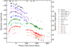 |
Fig. 2. Absolute magnitude (rest frame) light curves from ∼1800 to 18500 Å, including the Liverpool Telescope SDSS filters as triangles, the Swift UVOT filters as squares and the ZTF filters as circles. The black triangles at the top indicate the phases of available spectra. Phase = 0 (at peak ZTF g-band) is estimated in Sect. 3.2. The light curves in the different bands were shifted for illustration purposes. |
2.1.3. Liverpool Telescope photometry
The Liverpool Telescope (LT; Steele et al. 2004) has five filters (u, g, r, i and z) available for photometric measurements on the optical imager IO:O. Reduced data were provided using the standard IO:O pipeline.
We observed apparent magnitudes between 17 and 398 days post explosion and put them into the rest frame using the procedure outlined in Sect. 2.1.1. We list the resulting photometry in Table 1 and plot the resulting rest frame LT light curves together with the UVOT and ZTF light curves in Fig. 2.
2.2. Spectra
We acquired spectra with the SPectrograph for the Rapid Acquisition of Transients (SPRAT; Piascik et al. 2014) on the 2 m LT via the Transient Name Server (TNS)5, (Perez-Fournon et al. 2020), the Spectral Energy Distribution Machine (SEDM; Blagorodnova et al. 2018) on the Palomar 60 inch telescope (P60), the Double Beam Spectograph (DBSP; Oke & Gunn 1982) on the 200 inch Hale telescope (P200) at Palomar Observatory, the Low Resolution Imaging Spectrometer (LRIS; Oke et al. 1995) on the 10 m Keck I telescope and the Andalucia Faint Object Spectograph and Camera (ALFOSC)6 on the 2.56 m Nordic Optical Telescope (NOT). Table 2 lists available details about each of the spectra taken of SN 2020qlb.
Summary of SN 2020qlb spectroscopic observations.
SPRAT spectra were acquired and automatically reduced according to Liverpool Observatory procedures7. SEDM spectra were reduced according to Rigault et al. (2019). DBSP spectra were reduced using a PyRAF-based pipeline described by Bellm & Sesar (2016). The LRIS spectrum was reduced using LPipe as described by Perley (2019). ALFOSC spectra were reduced using PyNOT8. Each spectrum was calibrated against a spectrophotometric standard star. For the Keck spectrum at +461 days, we tied the flux scale to the host galaxy photometry. All spectra will be uploaded to WISEREP9.
In Fig. 3 we show sequential spectra from the different rest frame epochs together with relevant markings of important features. The noticeable gap between day +2 and day +109 includes a solar conjunction when ground based observations were not possible.
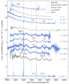 |
Fig. 3. Spectral sequence of SN 2020qlb. The dark blue SN 2020qlb spectra were smoothed using a Savitzky-Golay low pass filter. A lighter shade of blue is used for un-smoothed data and measurement errors. Spectra from a well studied SLSN-I (SN 2015bn) are shown in gray for comparison. P-Cygni profile minima used for velocity estimations are marked in dark red. Narrow host galaxy emission lines ([O III], Hα and [O II]) used for redshift estimation are indicated with green, red and blue vertical dashed lines. Blended Fe II absorption features, as well as [Mg I] and [Ca II] emission features are noted in black. Nebular phase [O I] and [O II] broad emission lines are noted in green. |
2.3. X-ray observations
While monitoring SN 2020qlb with UVOT, Swift also observed the field between 0.3 and 10 keV with its onboard X-ray telescope XRT in photon-counting mode (Burrows et al. 2005). We analyzed these data with the online-tools of the UK Swift team10 that use the methods described in Evans et al. (2007, 2009) and the software package HEASoft version 6.26.1.
SN 2020qlb evaded detection in all epochs. The median 3σ count-rate limit of all epochs is 0.007 count s−1 (spread: 0.003−0.03 count s−1) between 0.3−10 keV. Stacking all epochs pushes the 3σ count-rate limit to 0.0002 count s−1. To convert the count-rate limits into a flux, we assumed a power-law spectrum with a photon index Γ11 of 2 and a Galactic neutral hydrogen column density of 5.75 × 1020 cm−2 (HI4PI Collaboration 2016). Between 0.3−10 keV the median count-rate limits correspond to an unabsorbed flux of 2.9 × 10⁻¹³ erg cm−2 s−1 and luminosity of 2.0 × 1043 erg s−1 (if all observations are coadded); and 9.0 × 10⁻¹⁵ erg cm−2 s−1 and 6.2 × 1041 erg s−1 respectively (if dynamic rebinning is used).
2.4. Host galaxy photometry
We retrieved science-ready coadded images from the Sloan Digital Sky Survey data release 9 (SDSS DR9; Ahn et al. 2012), DESI Legacy Imaging Surveys (Legacy Surveys, LS; Dey et al. 2019) data release 8, and the Panoramic Survey Telescope and Rapid Response System (Pan-STARRS, PS1) DR1 (Chambers et al. 2016). We measured the brightness of the host using LAMBDAR12 (Lambda Adaptive Multi-Band Deblending Algorithm in R; Wright et al. 2016) and the methods described in Schulze et al. (2021). Table 3 lists the measurements in the different bands.
Host galaxy photometry. Magnitudes are not corrected for reddening.
3. Light curve analysis
In this section we analyze the light curves. We estimate the explosion date, the epoch of the maximum g-band flux, characteristic light curve timescales, and the g − r color evolution.
3.1. Explosion date estimation
To estimate the explosion date we first generated the flux light curves in Janskys from the observer frame arbitrary unit (DN) flux and zeropoint (ZP) magnitudes for the ZTF forced photometry data.
We fit a Heaviside function multiplied by a power law, as done in Miller et al. (2020), to the complete set of baseline and early g- and r-band measurements to estimate the explosion date to be MJD 59048.2 ± 1.8.
However, we found a better convergence by fitting (numpy.polyfit) a second order polynomial to both the first three r-band and to the first four g-band flux measurements that rise above the initial baseline values. Initially the g- and r-band fits both plotted earlier than their respective last baseline flux measurements, violating the upper limits these points provide. We therefore added the last baseline value for each filter band to the selected data points and refit the polynomials. The resulting fits are shown in Fig. 4.
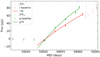 |
Fig. 4. ZTF r- and g-band flux in the observer frame near in time to the initial detection of SN 2020qlb. Points used for the second degree polynomial fits are darkened. |
We then ran a Monte-Carlo simulation of randomly selected data points from a Gaussian distribution of the one sigma uncertainties for each of the selected flux measurements. The resulting explosion date using the g filter was MJD 59050.68 ± 0.20 and for the r filter was MJD 59050.70 ± 0.34. By combining both filter solutions we estimate an explosion date of MJD 59050.69 ± 0.28.
The quoted error includes only the statistical uncertainty and not any systematic uncertainty terms. In practice, we have no constraints on the light curve below the ZTF detection limit (∼21.1 mag for ZTF g-band, corresponding to an absolute magnitude of g ∼ −18.3 mag). If SN 2020qlb had an initial bump, plateau phase or a different rising slope below this limit it would not be captured by our uncertainty estimate for the explosion date.
3.2. Peak g-band magnitude and light curve timescales
In order to estimate the peak g-band magnitude and corresponding phase, as well as different measures of the rise and decline time, we interpolate the light curve. Following Angus et al. (2019), we use Gaussian Process (GP) regression interpolation utilizing the Python package GEORGE (Ambikasaran et al. 2015) with a Matern 3/2 kernel.
The resulting ZTF g- and r-band interpolated light curves are shown in Fig. 5. We used the interpolated curve to determine that the peak g filter absolute magnitude occurred 77.1 days past explosion (MJD 59140.0). The maximum Mg was −22.25 ± 0.01 mag. We note that this estimate does not include any correction for potential host galaxy extinction (Sect. 9.2); if this is also included the peak g-band magnitude would be  mag.
mag.
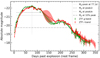 |
Fig. 5. GP interpolated ZTF-g and -r (rest frame) light curves. Horizontal lines used to calculate the different rise and decline times are plotted in gray. The ballooning effect of the GP interpolation algorithm is clearly seen in the solar conjunction gap in the data between 120 and 170 days past explosion. |
We then used the gray horizontal lines in Fig. 5 together with the GP interpolated Mg light curve to determine the rise and decline times. The rest frame rise time from half maximum was 48.6 ± 0.5 days, from 1/e maximum was 55.7 ± 0.4 days, and from 10% maximum was 72.4 ± 0.3 days. The rest frame decline time to half maximum was  days, to 1/e maximum was
  days, and to 10% maximum was 164 ± 2 days.
To determine where SN 2020qlb can be found in the phase space of rise time versus maximum absolute magnitude we plot the 69 SLSN-I from Chen et al. (2022b) in comparison with SN 2020qlb in Fig. 6. The rise time and peak brightness of SN 2020qlb are both high (94th and 89th percentiles respectively) among SLSNe-I, but not unprecedented.
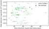 |
Fig. 6. Peak Mg versus e-folding rise time for 69 ZTF SLSNe-I from Chen et al. (2022b) are compared with SN 2020qlb. |
3.3. g − r color evolution
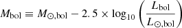
We also use the GP interpolated ZTF g- and r-band light curves to construct the g − r (color) magnitude evolution plot shown in comparison to a recent survey of SLSNe-I (Chen et al. 2022b) in Fig. 7. SN 2020qlb’s color evolution is one of the bluest but otherwise evolves normally compared to other SLSNe-I. We note that this color curve is calculated assuming zero host galaxy extinction; if this is included (Sect. 9.2 it would shift the color of SN 2020qlb even bluer by another 0.13 mag.
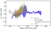 |
Fig. 7. SN 2020qlb g − r color evolution created from the ZTF-g and -r filter GP interpolations in Sect. 3.2 in blue and the g − r measurements with the LT in red. The gray background is a scatter plot of the 75 SLSNe-I and orange is for the 9 with 0.13 < z < 0.19 from Chen et al. (2022b, Fig. 13). |
4. Spectral analysis
In this section we analyze SN 2020qlb’s spectral evolution shown in Fig. 3 to estimate the host galaxy redshift, the SN spectral classification and the ejecta velocity evolution. We also note that there are no typical narrow lines which are signature spectral CSM interaction features (see Sect. 10.2.3) at any phase.
4.1. Host galaxy redshift
We determine the SN host galaxy redshift (z) by using the Hα line in the rest frame −28.5 d spectrum, the galaxy’s strong narrow forbidden [O III] transitions at 4959 Å and 5007 Å as well as the [O II] transition at 3727 Å. We thereby infer a redshift of z = 0.1583.
4.2. Spectral classification
We confirm the SLSN-I classification of SN 2020qlb by comparing the hot and cool photospheric phase (Gal-Yam 2019) spectra to well studied SLSN-I spectra.
In the upper three spectra in Fig. 3 we find the typical O II “W” feature around 4500 Å as well as a characteristic blue continuum. The three spectra from SN 2020qlb compare well with the hot photospheric phase spectrum from SLSN-I 2015bn at phase −27 days (Nicholl et al. 2016).
We also compare the lower four spectra from SN 2020qlb in Fig. 3 with two cool photospheric phase spectra from SLSN-I 2015bn. Prevalent matching features such as the [Mg I] and [Ca II] broad emission lines, noted in Fig. 3, indicate that SN 2020qlb evolved as a typical SLSN-I in the cool photospheric phase between phases +109 and +180.
4.3. P-Cygni velocity estimations
P-Cygni profiles were found in the SN 2020qlb photospheric phase spectra for the Si II, O II and O I lines marked in dark red in Fig. 3. We used these profiles to estimate the ejecta velocity according the longitudinal relativistic Doppler shift. We fit an equation consisting of a straight line component to match the continuum, and a Gaussian component to match the absorption feature to P-Cygni profile data using the scipy.optimize.curve_fit algorithm. The resulting λmin parameter fit values and covariance matrices were then used to produce absorption line velocity estimates and their propagated errors.
We find that the maximum velocity is ∼10 000 km s−1, the velocity near peak is ∼8000 − 10 000 km s−1 and ∼4000 − 6000 km s−1 at ≳100 days post-peak. Chen et al. (2022a, Fig. 1), in 56 events, find that SLSNe-I have typical near peak O II velocities of ∼12 000 km s−1, ranging between ∼6000 and ∼21 000 km s−1.
5. Photospheric temperature and radius
To measure the photospheric temperature and velocity evolutions we GP interpolate all light curves and extract the values at the time of the UVOT observations, and fit each epoch with a Planck function. We then utilize the scipy.optimize.minimize13 algorithm to fit a blackbody to the data at each of the 22 UVOT epochs, as well as the 17 full sets of LT data available at later epochs. The algorithm therein estimates the best-fit temperature and radius at each epoch including a one standard deviation error for both.
The optical data are adequately described by the Rayleigh-Jeans tail of the Planck function. However, the three UV filters are consistently incompatible with the best-fit blackbody function, which we attribute to line blanketing. We note that this effect is not uncommon in SLSNe (see e.g., Yan et al. 2017b); a similar choice is done by Nicholl (2018) in their SuperBol software. We therefore exclude these three filters when fitting the blackbody temperatures and radii. Figure 8 shows an example of the resulting blackbody fit to the selected data at phase −51.2 days relative to the Mg maximum.
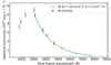 |
Fig. 8. Example (phase −51.2 days) of how a blackbody fit to photometric data is used to estimate the temperature and photospheric radius. The three UVOT UV filter measurements are excluded due to the UV line-blanketing effect. |
The resulting evolution of SN 2020qlb’s photospheric radius is plotted in Fig. 9. It is generally comparable to the 31 SLSNe-I from Chen et al. (2022b).
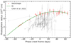 |
Fig. 9. Rest frame radius evolution of the SN photosphere from blackbody fits to data from UVOT epochs. A fourth degree polynomial was fit to the data. SLSN-I radius evolutions from Chen et al. (2022b) are shown in gray. |
We estimate the photosphere velocity evolution by plotting the derivative of the fourth degree polynomial fit of the radius evolution in Fig. 10 as well as the velocity estimates from the P-Cygni profiles from Sect. 4.3. A general convergence of the maximum velocity estimates in Fig. 10 appears to be ∼10 000 km s−1.
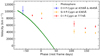 |
Fig. 10. Velocity evolution of the SN photosphere shown in green based on the fourth degree polynomial fit to the photosphere radius evolution shown in Fig. 9. P-Cygni absorption line velocity estimates from Sect. 4.3 are included as well. |
We also estimate SN 2020qlb’s temperature from spectra that were taken during the early photospheric phase of the SN. A blackbody was fit to the rest frame spectral data. The resulting temperature estimations are plotted in red in Fig. 11 together with the other temperature estimates in blue and orange as well as with the 31 SLSNe-I from the ZTF’s phase-I survey (Chen et al. 2022b) in light gray. SN 2020qlb’s temperature evolves similarly to most of the 31 SLSNe-I.
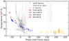 |
Fig. 11. Temperature evolution of the SN 2020qlb photosphere (blue: fit to UVOT + optical data; orange: fit to LT ugriz data; red: fit to spectra) in comparison to the 31 SLSN-I temperature evolutions from Chen et al. (2022b) shown in light gray. |
6. Bolometric light curve
To construct a bolometric light curve we first estimate SN 2020qlb’s spectral luminosity (Lλ) at all wavelengths at each epoch. The spectral energy distributions (SEDs) at each epoch are then integrated over all wavelengths to create the bolometric light curve.
6.1. Spectral energy distributions
Given a set of rest frame Lλs calculated from measurements in filters ranging from the UV to the visible we interpolate straight lines between data points. At wavelengths lower than the lowest filter wavelength and at wavelengths higher than the highest filter wavelength we use two similar sets of extrapolation methods.
At the 22 epochs where UVOT filter data is available we create the extrapolation short of the shortest wavelength by fitting a blackbody to LT’s u-band and the UVOT’s UV filters, while a blackbody fit to the optical bands is used to create the extrapolation long of the longest wavelength (see also Sect. 5). These methods are also used in SuperBol software as described by Nicholl (2018). Figure 12 shows an example of how the SED is constructed for phase −51.2 days from the Mg peak.
 |
Fig. 12. Example, at a phase of −51.2 days, of how an SED is constructed using linear interpolations between photometric data points and extrapolated on both ends as explained in the text. |
At later epochs where a complete set of the five LT filter data is available we use the extrapolation methods described by Lyman et al. (2014) to create the SEDs. These extrapolation methods differ from the SuperBol methods in that we draw a straight line between LT’s u-band and Lλ = 0 at 2000 Å on the side short of the shortest wavelengths. At additional epochs, where only 3 or 4 filter measurements are available, we use a GP interpolation (see Sect. 3.2) to estimate the missing filter magnitude(s) and error(s) before constructing the SEDs.
The maximum Lλ is encapsulated by the data at each epoch; an example of this is shown in Fig. 12. We therefore expect that a significant amount of the bolometric flux is included within the measurement ranges and that the two extrapolation methods to create the SEDs are accurately estimating the bolometric luminosities at their respective phases.
6.2. Bolometric luminosities
At each of the 39 epochs where SEDs were created (see Sect. 6.1) we calculated the bolometric luminosity by integrating over wavelength. We then performed a Monte Carlo simulation, using samplings from a normal distribution of the Lλ errors, to create error values for the luminosity estimates. The resulting plot of the bolometric luminosities and their errors over time are plotted in green (UVOT phases) and yellow (LT phases) in Fig. 13.
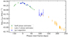 |
Fig. 13. Interpolated bolometric luminosities are shown interlaced with the bolometric luminosities estimated in Sect. 6.2. |
6.3. Bolometric interpolations
The ZTF has a higher cadence of measurement than the Swift/UVOT telescope. We therefore linearly interpolate luminosities at epochs between the bolometric data points created in Sect. 6.2.
Lyman et al. (2014) created analytic relationships to estimate bolometric light curves for different types of core collapse SNe by identifying correlations between different measurements of color, for example Mg − Mr ≡ (g − r), and a bolometric correction factor to the absolute magnitude in the g-band BCg ≡ Mbol − Mg, where Mbol is defined as follows:
where Lbol is the bolometric luminosity, L⊙, bol and M⊙, bol are the sun’s luminosity (L⊙, bol = 3.828 × 1033 erg s−1) and bolometric magnitude (M⊙, bol = 4.74 in the g-band; Mamajek et al. 2015).
Using the Swift and LT phase bolometric luminosities, interpolated ZTF-g and -r measurements as well as calculated absolute g-band magnitudes we plot BCg versus (g − r) as shown in Fig. 14. The first seven data points in Fig. 14 show no relationship between the plotted parameters, likely because at these early epochs the SED peaks sufficiently far into the UV so that the g − r color is not affected. We therefore exclude these epochs from our fit. A second degree polynomial using the scipy.optimize.curve_fit algorithm produces the fit (in blue) shown in Fig. 14 for the post-peak data.
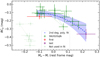 |
Fig. 14. Bolometric correction as a function of rest frame g − r color. A second degree polynomial curve-fit is compared to the post peak bolometric correction to the g-band (BCg) versus (g − r) color data. The data are shown connected in time sequence. The first seven points were removed from the curve-fit. |
The resulting relationship between BCg and (g − r) is:
We then used ZTF-g and -r measurements made after the phase of the last removed (g − r) value and where (g − r)< 0.3 to provide the interpolated bolometric luminosities plotted in blue in Fig. 13.
By integrating the entire bolometric light curve in Fig. 13 using a simple trapezoidal method we estimate the total radiated energy of SN 2002qlb to have been > 2.8 ± 0.05 × 1051 erg. Integrating only over the observed filters (i.e., no extrapolations at either the red or the blue end, and not extrapolating to the presumed explosion date, see Sect. 6.1) gives a strict lower limit on the total radiated energy of 2.1 × 1051 erg. We note that this bolometric light curve integration is calculated assuming zero host galaxy extinction; if this is included (see Sect. 9.2) the total radiated energy would be > 2.9 ± 0.1 × 1051 erg; and > 2.2 × 1051 erg if no extrapolations are used.
7. Light curve modeling
In this section, we use the light curves (observed and bolometric) as well as the measured velocity to compare SN 2020qlb to different semi-analytic models in order to determine the most likely power source.
7.1. Radioactive source model (Arnett)
Arnett (1982) presented a semianalytic model wherein the radioactive decay of 56Ni → 56Co → 56Fe emits gamma photons that diffuse through an expanding spherically symmetric and homologous SN ejecta and escape near the photosphere. The output luminosity is given as (Nicholl et al. 2017, Eq. (5)):

where P(t′) is the source input power, a function of the SN’s 56Ni mass, as shown in Cano et al. (2017, Appendix A); tleak is a characteristic time parameter for the eventual leakage of gamma photons (Sollerman et al. 1998); and τdiff is the effective diffusion time of the SN,
where κ is the opacity (e.g., 0.2 cm2 g−1 assuming only electron scattering in a hydrogen free environment) and β is an integration constant of the source density profile (≈13.8).
We use the lmfit.minimize14 algorithm’s least square method to fit critical parameters (Mej, M56Ni and tleak). The best fit Arnett model is shown in Fig. 15. The resulting parameter values for the Arnett radioactive source model are: Mej = 11 ± 1 M⊙, M56Ni = 34 ± 1 M⊙, vej = 1 × 10⁴ km s−1 (see Sect. 4.3), Ek = 6 ± 1 × 1051 erg, tleak = 160 ± 4 days and the diffusion timescale (see Eq. (5)) is 54 days. Since the total ejecta mass includes the mass of the 56Ni, the parameter results of Mej = 11 M⊙ and M56Ni = 34 M⊙ are therefore unphysical. We note that reparametrizing the 56Ni mass as a fraction of the ejecta mass, so that the result is forced to be physical, converges to a poor fit (see Fig. 15).
 |
Fig. 15. Bolometric light curve plotted together with the best-fit magnetar and Arnett radioactive source models. Forcing the 56Ni mass to be less than or equal to the ejecta mass results in the red dashdot line. |
7.2. Magnetar source model
In this subsection we use a maximum likelihood method, using the least squares technique, to fit the bolometric light curve. We then compare the results to a fit of the observed multi-band light curves using a Markov chain Monte Carlo (MCMC) technique to analyze how well a magnetar can power SN 2020qlb.
7.2.1. Fit to bolometric light curve
Assuming that the central power source of the SN is from the dipole spindown energy deposition of a magnetar, Inserra et al. (2013) proposed that the power function P(t′) to be used in Eq. (4) should be as follows:
where B14 is the dipolar magnetic field strength in 1014 G, Pms is the initial spin period in milliseconds, and the magnetar spin-down timescale τp is given as follows:
The diffusion timescale τdiff can be rewritten as
where the kinetic energy of the SN ejecta Ek is estimated assuming a homologous and spherically symmetric ejecta, with constant density, as
where vej is the maximum ejecta velocity.
Given a set of reasonable parameter (uniform) priors we fit the magnetar model using the lmfit.minimize least squares method to determine the best fit parameter values to be Mej = 30 ± 2 M⊙, B14 = 0.88 ± 0.03, Pms = 1.4 ± 0.1, vej = 1 × 10⁴ km s−1 (see Sect. 4.3), tleak = 309 days, and the diffusion timescale (see Eq. (8)) is 86 days. The resulting best fit parameter model is plotted together with the bolometric light curve in Fig. 15.
7.2.2. Fit to multiband data
We also employed an alternative method to estimate magnetar model parameters called the Modular Open Source Fitter for Transients code (MOSFiT; Guillochon et al. 2018; Nicholl et al. 2017). After inputting the SN redshift, all observer frame light curve data, filter information as well as reasonable priors, MOSFiT runs a MCMC process to determine the posterior distributions for 12 different parameters pertinent to a magnetar power source for the SLSN. We present the relevant results of MOSFiT for SN 2020qlb in Table 4 together with the results from Sect. 7.2.1. The MOSFiT light curve fit is shown is Fig. 16 and the posteriors are shown in Fig. 17.
Comparison of two methods for magnetar modeling and their best fit (median and 1σ) parameters.
 |
Fig. 16. Multi-band light curve of SN 2020qlb inferred from the magnetar-model, with bands offset for clarity. The colored lines show the range of most likely models generated by MOSFiT. Phase = 0 is where the ZTF g-band is maximized in the observer frame (MJD 59140.0). |
 |
Fig. 17. 1D and 2D posterior distributions of the magnetar model parameters from the MOSFiT model. Median and 1σ values are marked and labeled. These are used as the best fit values. |
We find good agreement between the values of AV, host, κ, and vej assumed for our least squares fit and those found by MOSFiT, as well as between Tmin found by MOSFiT and the late-time photospheric temperature calculated in Sect. 5 (see Fig. 11). We also find the posteriors of both MNS and Pspin peak close to the edges of their respective priors, which are informed by conservative estimates of the Tolman-Oppenheimer-Volkoff (TOV) limit and mass-shedding limit respectively. This means that we herein find this system to contain a magnetar close to its maximum mass spinning at close to its breakup velocity.
Both the MOSFiT and least squares methods estimate the kinetic energy using Eq. (9) to be approximately 2 × 1052 erg.
The total amount of rotational energy stored in a magnetar is estimated by Kasen (2017) as
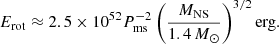
The MOSFiT method thereby estimates the available rotational energy to power the SN light curve to be 4.0 × 1052 erg while the least squares method (with MNS = 1.97 M⊙) only predicts it to be 2.1 × 1052 erg. However, both of these values are well above the total integrated light curve radiated energy of 2.8 ± 0.3 × 1051 erg (see Sect. 6.3).
The magnetar spin-down timescales calculated via the Least-Squares and MOSFiT methods are 3.8 and 4.0 days respectively, while the diffusion timescales are 86 and 82 days respectively. Suzuki & Maeda (2021) show that if the spin-down and diffusion timescales are comparable, then a large fraction of the rotational energy is expected to be contributed to the SN luminosity, which is typical for SLSNe. If the spin-down timescale is much shorter than the diffusion timescale then most of the energy is expected to be contributed to the kinetic energy, which is more typical for SN Ic-BL. From supernova surveys and modeling efforts, the average SLSN-I rise time (which is roughly the diffusion time) is ∼40 days (Chen et al. 2022b) and spin-down timescale is ∼15 days (Nicholl et al. 2017; Chen et al. 2022a), a factor of ∼2−3; while the average rise time of a SN Ic-BL is ∼15 days (Taddia et al. 2019), and they are usually modeled with spin-down timescales of ∼ an hour (Suzuki & Maeda 2021), a factor of > 100. Both fitting methods give τdiff/τp ∼ 20 for SN 2020qlb, which is intermediate between typical SLSNe-I and SNe Ic-BL, and is consistent with a large fraction of the rotational energy being converted to kinetic energy in this SN.
7.2.3. Predicted radio and soft X-ray counterparts
Radio observations can provide an interesting clue as to the nature of the supernova power source, as both a magnetar engine (Murase et al. 2016; Omand et al. 2018) and CSM interaction (Chandra 2018) can produce radio emission, but on different timescales and with different spectra. Three SLSNe-I have already been detected in radio: PTF10hgi (Eftekhari et al. 2019; Law et al. 2019; Mondal et al. 2020; Hatsukade et al. 2021), which is consistent with the magnetar model; SN 2017ens (Coppejans et al. 2021a), which transitioned from BL-Ic to SLSN and is likely powered by a combination of a magnetar and CSM interaction (Chen et al. 2018); and SN 2020tcw (Coppejans et al. 2021b), which was detected only a few months after explosion and is likely due to a CSM interaction.
We use the magnetar parameters found from the MOSFiT models in Sect. 7.2.2 to calculate the expected radio emission for SN 2020qlb. We use the model previously presented in Omand et al. (2018), Law et al. (2019), Eftekhari et al. (2021), which assumes pulsar wind nebula (PWN) microphysics calibrated to the Crab Nebula (Tanaka & Takahara 2010, 2013), which has a broken power-law electron injection spectrum with an injection Lorentz factor γb = 6 × 10⁵ and spectral indices q1 = 1.5 and q2 = 2.5. In Fig. 18 we show the predicted light curves at 3, 15, and 100 GHz, which correspond to VLA bands S and Ku and ALMA band 3, respectively. Since the ionization state of the ejecta is not fully understood, we use free-free absorption estimates based on an un-ionized (dashed lines) and fully singly-ionized (solid lines) ejecta as two extreme cases.
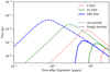 |
Fig. 18. Predicted radio emission for SN 2020qlb at 3 (red), 15 (green), and 100 (blue) GHz. The dashed and solid lines represent estimates of free-free absorption using an un-ionized and singly ionized oxygen ejecta, respectively. |
Previous observations with VLA and ALMA (e.g., Law et al. 2019; Eftekhari et al. 2021; Murase et al. 2021) have usually had noise levels of about 10 μJy, while SN 2020qlb is only expected to reach ∼1 μJy for an un-ionized ejecta and 0.1 μJy for a singly ionized ejecta, so it is likely not a good candidate for radio follow-up. Additionally, changing the microphysics of the PWN could result in either a low-magnetization Compton-dominated nebula or a high-magnetization synchrotron-dominated nebula (Vurm & Metzger 2021; Murase et al. 2021), which both result in a decrease in radio emission and an increase in gamma-ray emission, making the object even harder to detect.
For soft X-rays, the main absorption process at 0.3−10 keV is photoelectric absorption which has an optical depth that can be expressed as τ = KρR. ρ is the ejecta density, R is the ejecta radius, and K is a mass attenuation coefficient that can be estimated as 2.5 cm2 g−1 (Z/6)3(Eγ/10 keV)−3, where Z is the average atomic number and Eγ is the photon energy (Murase et al. 2015; Kashiyama et al. 2016). For SN 2020qlb, we find τ ≈ 5 × 10⁶ (t/day)−2 (Eγ/10 keV)−3, so soft X-rays are not expected to be able to escape for ≳5 years. The X-rays can also escape if the ejecta is completely ionized (Metzger et al. 2014), but that is unlikely to happen for SLSNe with more massive ejecta, such as SN 2020qlb.
8. Light curve undulations
One striking feature of SN 2020qlb is its light curve undulations. Despite similar findings in other SLSNe (e.g., Inserra et al. 2017; Nicholl et al. 2016), the physical mechanisms behind the so-called bumps are not well understood. In this section, we analyze the light curve undulations present in SN 2020qlb (amplitudes, timescales); their interpretation is discussed in Sect. 10.3.
To characterize the undulations, we first subtracted from each filter a polynomial fit capturing the large-scale shape of the light curves. We chose the lowest-order polynomial that still fits the overall shape; for most filters a third-degree polynomial was sufficient, while the two ZTF filters required a fifth-order one. Figure 19 shows the resulting residual light curves.
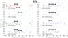 |
Fig. 19. Light curve residuals after subtracting a polynomial (order indicated in each panel) to the first 200 days of data. Visual inspection indicates fluctuations with an approximate timescale of ∼30 days in all filters; this is indicated in each subplot with an arrow showing time between peaks/troughs. |
Visual inspection of each subplot in Fig. 19 shows residual fluctuations in all filters. The typical timescale (peak to peak or trough to trough) appears to be about 30 days; these are highlighted with arrows on the figure. The fact that the arrows generally match across filters suggests that the undulations are approximately monochromatic.
To better quantify the timescales of the undulations, we analyzed the bolometric light curve. At each of the phases we calculated the residual between the bolometric light curve and the best fit magnetar model. The least squares method method was selected since it utilized the constructed bolometric light curve to identify the best magnetar model fit. The resulting residual is shown in Fig. 20; visual inspection suggests an oscillatory appearance for the first 150 days. A GP interpolation of the residual is also shown in dark blue. The center maximum, of the three GP interpolation maxima, matches the peak Mg phase indicating that the undulation is included in the maximum brightness determination. We also note that the peak of the magnetar model (marked in orange) is at a phase of −19.4 days.
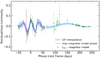 |
Fig. 20. Bolometric light curve less magnetar residual and the GP interpolation of the residual, both normalized by the maximum magnetar model luminosity. The phase of the magnetar model maximum (−19.4 days) is marked with a vertical line for reference. |
In order to identify the timescale of the undulations in the GP interpolated residual we performed a discrete fast Fourier transform (FFT) using the scipy.fftpack.fft15 algorithm to create a periodogram of the underlying frequencies in the residual. Figure 21 shows that a timescale of approximately 32 ± 6 days is present in the residual, which matches well what is seen by eye in the individual filter residuals in Fig. 19.
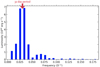 |
Fig. 21. Fast Fourier transform of the GP interpolation of the bolometric LC less magnetar model residual for phases up to +60 days as shown in darker blue in Fig. 20. |
The energy scale of the undulations is estimated by the residual’s maximum amplitude of approximately 1.7 × 1043 erg s−1. This is about 6% of the peak bolometric luminosity of 2.6 × 1044 erg s−1.
We also observe an additional bump in the residual between phases of +100 and +180 days in Fig. 20. A GP interpolation for this time period is shown in light blue as well. This late-time bump appears to have a lower amplitude and a longer timescale than the earlier ones.
Light curve bumps have been discovered in many other SLSNe-I. Hosseinzadeh et al. (2022) found bumps or undulations in 44−76% of the post peak light curves of 34 SLSNe. Similarly, Chen et al. (2022b) observed that 39%−66% of 77 SLSNe-I from the ZTF-I operation had undulations with an average duration of 21 days and an average amplitude of 4% of maximum brightness.
9. Host galaxy
As seen in Fig. 1, the host galaxy of SN 2020qlb appears to be a faint, blue dwarf galaxy. In this section, we discuss the properties of the galaxy in more detail, and put it in context of the population of SLSN-I host galaxies.
9.1. HST image and morphology
SN 2020qlb was observed by the Hubble Space Telescope (HST) WFC3/UVIS on January 7, 2022, as part of Snapshot program 16657 (PI: Fremling), corresponding to a phase of +367 rest-frame days past g-band maximum. The image in Fig. 22 is taken in F336W, with a corresponding rest-frame effective wavelength of 2900 Å. We see two bright knots of emission, with the supernova location corresponding to the northern knot as indicated by the arrow. The total systematic astrometric uncertainty, dominated by the ZTF, is about 0.1 arcsec. With more stars in the UVIS image we could have made a more precise astronometric matching to better determine the exact supernova location within the galaxy. We note that this kind of morphology, which could be either an interacting system or a dwarf galaxy with multiple regions of strong star formation, is not unusual among SLSN-I host galaxies (Lunnan et al. 2015; Ørum et al. 2020).
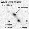 |
Fig. 22. HST image of the host galaxy of SN 2020qlb, corresponding to a rest-frame wavelength of 2900 Å, and taken at a phase of +386 days past the g-band peak. The host galaxy appears to have two knots of emission, with the supernova located at the northern knot. The apparent point source could include supernova emission, or be a star-forming region in the host galaxy; a template image would be needed to tell the two apart. The source visible in the bottom left of the image is caused by a cosmic ray. |
We also note that the northern knot appears, by eye, to consist of a point source on top of more extended emission. This point source could be UV light from the supernova still visible at +367 days; PSF photometry yields an apparent magnitude 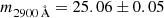 mag, which corresponds to an absolute magnitude of
 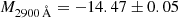 mag. However, to truly ascertain whether this is supernova light or simply a brighter region within the host galaxy would require a second epoch of HST imaging in order to do proper host subtraction.
9.2. Emission line diagnostics
The Keck spectrum taken at a phase +461 days past maximum (see Fig. 3) is dominated by host galaxy light, and contains a wealth of emission lines that can be used to analyze the properties of the underlying H II region. We measure emission line fluxes by fitting Gaussian profiles to the (generally unresolved) host galaxy lines; the results are listed in Table 5.
Observed host galaxy emission line fluxes, uncorrected for MW dust extinction.
After correcting for Milky Way extinction, we measure a Balmer decrement Hα/Hβ = 3.20 ± 0.16, indicating moderate host galaxy extinction. Assuming intrinsic ratios corresponding to Case B recombination (Osterbrock 1989), we derive a contribution E(B − V)host = 0.10 ± 0.05 mag.
We marginally detect the auroral [O III]λ4363 line, allowing for the electron temperature to be calculated and the oxygen abundance to be measured directly. We use the Python package PyNeb (Luridiana et al. 2013) to iteratively calculate the O++ electron temperature and the electron density ne from the ratios of [O III]λ4363/[O III]λ5007 and [S II]λ6731/[S II]λ6717, respectively. The O+ electron temperature is then obtained assuming the relation

where  and
and  are in units of 10 000 K (Campbell et al. 1986). We then use the ratios of [O III]λ5007/[O III]λ4959 and [O II]λ3727/Hβ to calculate the O++/H and O+/H abundances, respectively, again using PyNeb. The final oxygen abundance is obtained from summing these two contributions. Using a Monte Carlo approach to resample the fluxes within their errors to calculate the uncertainty, we obtain a final metallicity of 12 + log(O/H)=8.0 ± 0.2 dex. Taking the solar oxygen abundance to be 12 + log(O/H)=8.69 ± 0.05 dex (Asplund et al. 2009), this corresponds to a metallicity of Z ≃ 0.2 Z⊙.
Using the extinction-corrected Hα flux, we can also calculate a star formation rate using the relation  (Kennicutt 1998). This yields a star formation rate of 1.4 M⊙ yr−1 for the host galaxy of SN 2020qlb. We note that this estimate is based on a spectrum (+461 days) that did not have contemporaneous calibration photometry but was calibrated using host galaxy photometry.
9.3. Host SED modeling
Figure 23 shows the observed host galaxy SED from 3000 to 10 000 Å. We modeled the SED with the software package Prospector version 1.1 (Leja et al. 2017) which uses the Flexible Stellar Population Synthesis (FSPS) code (Conroy et al. 2009) to generate the underlying physical model and python-fsps (Foreman-Mackey et al. 2014) to interface with FSPS in Python. The FSPS code also accounts for the contribution from the diffuse gas (e.g., H II regions) based on the Cloudy models from Byler et al. (2017). Furthermore, we assumed a Chabrier initial mass function (Chabrier 2003) and approximated the star formation history (SFH) by a linearly increasing SFH at early times followed by an exponential decline at late times (functional form t × exp(−t/τ)). The model was attenuated with the Calzetti et al. (2000) model.
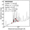 |
Fig. 23. Spectral energy distribution (SED) of the SN 2020qlb host galaxy from 1000 to 60 000 Å (black data points, Table 3). The solid line displays the best-fitting model of the SED. The red squares represent the model-predicted magnitudes. The fitting parameters are shown in the upper-left corner. The abbreviation “n.o.f.” stands for numbers of filters. |
The best fit, shown in gray in Fig. 23, suggests a low-mass star-forming galaxy with a mass of  and a star formation rate of
  yr−1. The mass and the star formation rate are in the expected parameter space of host galaxies of SLSNe-I at similar redshifts (Perley et al. 2016; Schulze et al. 2018) albeit in the lower half. The attenuation inferred from the SED modeling is broadly consistent with what is obtained from the Balmer decrement (Sect. 9.2).
10. Discussion
In this section we begin by discussing and comparing SN 2020qlb to the unique criteria and general characteristics of SLSNe-I as described by Howell et al. (2017) and Gal-Yam (2019). Potential light curve power sources are then discussed, followed by a review of possible undulation power sources.
10.1. SLSN-I concordance
In this subsection we discuss the distinctive characteristics of SLSNe-I based on their four phases as presented by Gal-Yam (2019): 1. Early bump, 2. Hot photosphere, 3. Cool photosphere, 4. Nebular. We therein discuss how SN 2020qlb compares to each typical property.
Chen et al. (2022a) found an early bump in 3/15 (6−44% with confidence limit of 95%) SLSNe-I from their ZTF Phase-I survey with at least four epochs of prepeak photometry. SN 2020qlb’s lack of an early light curve bump is therefore not unusual.
SLSN rise times, that is to say from explosion to the luminosity peak, typically range from ∼20 to > 100 days in the rest frame of the SN (Gal-Yam 2019). SLSN light curve rise times from 1/e maximum to peak are typically between ∼15 and > 60 days (see Fig. 6). SN 2020qlb’s 77.1 day rise time from explosion to peak, although on the longer side, is therefore typical for a SLSN-I (Fig. 6).
Similarly, the peak luminosity of SN 2020qlb is shown on Fig. 6 compared to the ZTF-I sample of Chen et al. (2022b). With a peak g-band absolute magnitude of Mg = −22.25 ± 0.01 mag, SN 2020qlb is in the upper range of typical SLSNe, and well above any threshold to be considered superluminous (Quimby et al. 2018; Gal-Yam 2019).
The hot photospheric phase, which includes the peak, is characterized by a hot (blue) spectral continuum with decreasing blackbody temperatures of up to 20 000 K, which is indeed what we find for SN 2020qlb in Fig. 11. Several absorption features (O I, O II and C II) are detected on top of the continuum. In particular, O II absorption features in the blue part of the visible spectrum are unique to SLSNe-I and are found persistently prior to the peak (Gal-Yam 2019). As discussed in Sect. 4.2, SN 2020qlb has the typical O II “W” feature near 4500 Å in its early spectra. Expansion velocities derived from the P-Cygni line profiles of O I, O II, Fe II et al. during the hot photospheric phase are typically estimated to be between 10 000 and 15 000 km s−1 (Quimby et al. 2018; Gal-Yam 2019). In Fig. 10, SN 2020qlb has an early velocity of ∼10 000 km s−1.
During the cool photospheric phase the photosphere cools and expands while the spectrum evolves to resemble typical Type Ic SN spectra. Meanwhile the unique O II features from the hot photospheric phase weaken as the temperature typically falls below ∼12 000 K (Gal-Yam 2019). In Sect. 4.2 we show how SN 2020qlb’s late spectra are typical for SLSNe-I.
The host galaxy of SN 2020qlb is also quite typical of SLSN-I host galaxies, with a low mass (log(M/M⊙)≃7.5), low metallicity (12 + log(O/H)≃8.0, direct method), and a high star formation rate ( yr−1). These are all within the typical range of SLSN-I host galaxies at this redshift, albeit at the more extreme end (e.g., Lunnan et al. 2014; Leloudas et al. 2015; Perley et al. 2016; Chen et al. 2017; Schulze et al. 2018, 2021).
SN 2020qlb clearly meets important criteria regarding brightness, spectral features and evolution. And since no characteristic is counter-indicative, we find that SN 2020qlb is a typical SLSN-1.
10.2. Light curve power source
10.2.1. Radioactive decay
Given the extreme level of SN 2020qlb’s brightness it is possible to suspect a power source wherein a e−/e+ pair-production instability SN (PISN) explosion could annihilate the progenitor star completely. Kasen et al. (2011) show that models of stars with initial masses in the range of 140 M⊙–260 M⊙ die in thermonuclear runaway explosions resulting in the synthesis of up to 40 M⊙ of 56Ni. The best fit radioactivity model shown in Fig. 15 estimates that 34 ± 1 M⊙ of 56Ni is required to explain the SN 2020qlb bolometric light curve, an amount within the PISN model prediction.
The Arnett 56Ni radioactive decay model fitting done in Sect. 7.1 estimates Mej, vej, M56Ni and tleak. vej is normally measured from high resolution spectra (see Sect. 5). The diffusion time τdiff (see Eq. (5)) describes the characteristic time frame for light to diffuse through the expanding ejecta and is calculated using both Mej and vej. The gamma photon leakage time tleak is given by Clocchiatti & Wheeler (1997) as  . So, in essence, the Arnett radioactive decay model only has two characteristic parameters, Mej and M56Ni. However, for SN 2020qlb the 56Ni mass is estimated to be significantly more than the ejecta mass (see Sect. 7.1). Since this is unphysical we discard the Arnett model describing a 56Ni radioactive source. The same argument requires us to discard the PISN radioactivity model as well.
10.2.2. Magnetar
The magnetar model fitting done in Sect. 7.2 is also able to trace the bolometric light curve. The MOSFiT MCMC method tests ranges of values for parameters that are assumed constant in the least squares fitting method. Table 4 indicates how the two methods compare for key parameters such as Mej, Pms, B14 and vej. By combining Mej and vej into one parameter EKE, the two methods achieve better agreement. So, in essence, the magnetar model has three characteristic parameters which are capable of reproducing SN 2020qlb’s light curve, that is Pms, B14, and EKE. Nicholl et al. (2017) present MOSFiT results for 38 SLSNe-I wherein median value ranges for  and
and  as well as the total range for EKE = 0.55 to 25.06 × 1051 erg all span the results of SN 2020qlb in Table 4. The soft X-ray nondetections (see Sects. 2.3 and 7.2.3) are also consistent with the magnetar model. We note that radio observations (see Sect. 7.2.3) could be used as a potential test of this scenario, but the predicted fluxes are too low for current radio interferometers.
The model for the smooth spin-down of a magnetar can only impart its rotational energy into the bolometric light curve in a smooth way. It therefore can only trace the general shape of the light curve and not the undulations as discussed in Sect. 8. Eventual magnetar-powered undulations not captured by the model are discussed in Sect. 10.3.1.
Given that each of the parameter estimates are within physically possible ranges (see Sect. 7.2.2) the magnetar model is retained.
10.2.3. CSM interaction
An additional potential external power source of SN light curves is the collisional interaction of the SN ejecta with circumstellar material (CSM). Strong shocks can convert the ejecta’s kinetic energy into radiation energy. The CSM can potentially result from stellar winds, binary mergers or interaction, or stellar eruptions (see Smith 2014).
Gal-Yam (2019) indicates that most CSM interacting SNe have strong and narrow emission lines as encountered in the spectra of H-rich Type IIn (n refers to “narrow”), He-rich Type Ibn, Ia-CSM and some Ic SNe. However, a lack of narrow lines does not always imply a noninteracting SN (see e.g., Type II-L SN 1979C and SLSN II SN 2008es Fransson et al. 1984; Bhirombhakdi et al. 2019). There are a few examples of CSM interaction in SLSNe-I noted by Yan et al. (2017a). However, as noted in Sect. 4, we find no such signature spectral features for SN 2020qlb as shown in Fig. 3.
Gal-Yam (2019) writes that there are no existing published models employing CSM interaction power that can fit SLSN-I spectra. However, there have been efforts to fit SLSN light curves with CSM interaction models. Hybrid, for example CSM plus radioactive decay, models such as the semianalytic model MINIM (Chatzopoulos et al. 2013) employ both SN and CSM parameters in a χ2 minimization fit. The increased number of available parameters in CSM interaction models should enable bolometric light curves to be reproduced very well. Liu et al. (2018) show that by increasing the number of CSM interactions it is possible to model even complex light curves, for example iPTF15esb and iPTF13dcc. In addition, Liu et al. (2018, Fig. 1) show how a triple ejecta CSM (in total ∼4 M⊙) interaction can fit the undulating bolometric light curve of iPTF15esb. In essence any light curve could eventually be fitted with multiple CSM interactions of different magnitudes occurring at different times.
We used MOSFiT to perform two CSM model (Chatzopoulos et al. 2013; Villar et al. 2017; Jiang et al. 2020) fits using two different kinds of CSM by setting the slope of the CSM density profile to be s = 0 (indicative of a constant density shell) and s = 2 (indicative of an r−2 steady state wind). Both fits yielded unphysically massive CSM compared to the ejecta mass, with 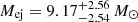 and
and 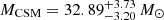 for the s = 0 model and
 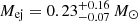 and
and  for the s = 2 model. However, parameters from semi-analytic models, such as the one employed by MOSFiT, are known to be inconsistent with those found by numerical approaches (Moriya et al. 2013, 2018; Sorokina et al. 2016), and can only be properly determined from non-LTE radiation hydrodynamical modeling (Chatzopoulos et al. 2013). Thus, even though our fit parameters were unphysical, we do not outright reject the CSM interaction scenario because of this.
Janka (2012) finds that SN explosion models driven by neutrinos are unlikely to explain SN energies above ∼2 × 1051 erg. However, we estimate that the total kinetic energy of SN 2020qlb is ∼2 × 1052 erg (see Sect. 7.2.2). Since CSM interaction can only draw its energy from the kinetic energy, and given that the explosion mechanism in an ejecta-CSM interaction powered-SN is neutrino-driven, it is unlikely to be the main power source of SN 2020qlb’s light curve unless a magnetar is also present to supply the necessary additional energy.
One could expect X-rays from the shock created by the interaction, similar to what has been seen for Type IIn supernovae (e.g., Chandra et al. 2015; Katsuda et al. 2016). In soft X-rays, this emission should be dominated by line emission. The strength of the emission also depends heavily on whether the shock is radiative or adiabatic, the CSM profile, the shock velocity, and other things for which we have no constraints. Also, unlike Type IIn SNe, the shock should be surrounded by metal-rich CSM, which may absorb X-rays up to two orders of magnitude more efficiently. From this, we find that an X-ray nondetection also seems consistent with the CSM interaction model. However, getting any meaningful constraints on physical parameters from our observed X-ray upper limit is unlikely.
Given the success of the magnetar model, the lack of spectral evidence for CSM interaction, unphysical fit parameters, energy considerations, as well as the large number of required CSM parameters we tentatively reject the CSM model as the primary light curve power source.
10.3. Undulation source
The magnetar model fits the general shape of SN 2020qlb’s light curve wherein undulating residuals remain. In this section we discuss possible mechanisms behind the observed modulation.
In Sect. 8 we determine that SN 2020qlb has more than two full periods of 32 ± 6 day undulations in the magnetar model residual near the peak of the bolometric light curve. The amplitude of the undulations was approximately 1.7 × 1043 erg s−1 which is roughly 6% of the peak bolometric luminosity. Another highly sampled SLSN-I, SN 2015bn (Fig. 24 Nicholl et al. 2016), also had more than two full periods of magnetar residual undulations. SN 2015bn, with a 30−50 day period oscillation amplitude of about 2.5 × 1043 erg s−1 which is roughly 11% of its peak bolometric luminosity, is similar to SN 2020qlb with regard to its magnetar residual undulations. Intriguingly, both have two to three oscillations near peak brightness with timescales in the order of 30 days, and with roughly similar amplitudes.
In the following subsections we consider the source of the observed undulating magnetar residuals grouped into four possibilities: (1) variations in the centrally located power source, (2) variations in the SN ejecta properties, (3) interactions with varying CSM densities, or (4) the eventual breakdown of model assumptions.
10.3.1. Central source fluctuations
Eventual central engine luminosity fluctuations will be stretched and delayed as they move through the homologous SN ejecta. The diffusion of photons through the ejecta thereby acts as a low-pass filter on any variable source. Central variations on short timescales compared to the timescale of the ejecta are therefore not expected to be observed at the SN photosphere.
One proposed central source for the undulations is suggested by Metzger et al. (2018) wherein fallback accretion onto the SN’s central compact object could provide additional luminosity. The accretion rate is predicted to have a time dependence of 1/(1 + t/tfb)5/3, where tfb is the fall-back timescale, which is different than the magnetar’s luminosity time dependence (see Eq. (6)).
A second possibility involves the eventual variability of the magnetar. Denissenya et al. (2021) discovered a local Milky Way magnetar (SGR1935+2154), the source of two fast radio bursts (FRBs), that showed a 231 day periodic windowed behavior (PWB) between epochs of activity and inactivity. Younger magnetars with significantly shorter spin periods could conceivably contain shorter periodic behavior as well, for example a 32 day pulsation.
Chugai & Utrobin (2022) and Moriya et al. (2022) suggest a third possibility wherein a post-maximum enhancement of the central magnetar’s dipole field or the thermalization parameter (how much magnetar energy is converted into SN thermal energy) could cause a light curve bump. We note that the physical mechanism behind the enhancement is not yet known, that Moriya et al. (2022) predict an increase in photospheric temperature that is not detected in SN 2020qlb, and that Chugai & Utrobin (2022) only claim to explain a single bump.
However it is difficult, if not impossible, for a pulsating central source on a scale of 32 days to diffuse through an ejecta with a diffusion timescale of 86 days (see Sect. 7.2.1). Following Hosseinzadeh et al. (2022, Eq. (8); shown here in Eq. (12)) we can constrain the depth from where a bump is produced. δ-parameter values,
rule out a central source of a light curve bump, where tbump is the time of the bump, Δt is the bump duration (one period), and trise is the rise time from explosion to peak.
When applying this rule of thumb to SN 2020qlb’s three residual maxima (at tbump = 44, 76 and 108 days post explosion) we calculate the δ-parameter to be 0.24, 0.41 and 0.59. The fluctuation source(s) must therefore be well away from the center. We thereby, given the model assumptions, rule out any centrally located undulation source. See Sect. 10.3.4 for a discussion about possible assumption breakdowns.
10.3.2. Ejecta property variations
Fluctuations are seen in all filter bands as well as the bolometric light curve (see Figs. 13 and 19). No 30 day fluctuations are seen in the g − r color evolution plot (Fig. 7). These observations therefore suggest that there is no apparent wavelength dependence of the magnetar residual undulations.
In Fig. 24 we plot the residuals from the fourth power of the temperature (T4) and a fitted third degree polynomial, relative to the fourth power of the zero phase temperature (11 366 K) estimate. There are hints of small temperature bumps at −30, zero and +30 to +40 post peak days, including a three sigma drop between −23 and −12 days which matches a bolometric residual trough. However, within the uncertainties and in general, it is not clear that temperature changes match the bolometric light curve fluctuations.
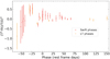 |
Fig. 24. T4 third degree polynomial residual relative to the zero phase T4 in red at Swift phases and in orange at LT phases. |
Kasen & Bildsten (2010) hypothesize that magnetar winds could sweep up most of the ejecta into a dense shell with uniform velocity and a sharp temperature jump at the edge. The post peak receding photosphere would get hotter as it crosses this temperature jump adding luminosity to the light curve. This scenario could give credence to a single light curve bump (or a plateau), but not to the cyclic undulations as observed. We therefore rule out this temperature jump hypothesis for SN 2020qlb.
Metzger et al. (2014) suggest that the magnetar wind nebula could inject electron/positron pairs into the base of the ejecta which would cool via Compton scattering and synchrotron emission. The resulting X-rays could ionize the inner portion of the SN ejecta forming ionization fronts which could propagate outward. Given the right conditions a front could break through the SN photosphere releasing unattenuated luminosity in both the optical/UV and soft X-ray bands. For instance, if an O II layer breaks through, the opacity to UV photons would be reduced. The additional leakage of UV photons through the photosphere could then disproportionately affect shorter wavelength UV observations. Given the lack of evidence for wavelength dependence of the undulations, and the nondetection of X-rays from 0.3−10 keV, we tentatively reject this hypothesis.
Nicholl et al. (2016) note the possibility that central overpressure from a magnetar could drive a second shock wave through the expanding ejecta which could break through the SN photosphere at large radii. Estimates suggest that the effects of this mechanism should be comparably weak and occur typically within 20 days after explosion. Since this secondary shock wave hypothesis would also result in a single perturbation we rule it out for SN 2020qlb.
Each of the above hypotheses essentially involves changes in the SN ejecta to create a light curve perturbation. In order to become more credible it will be necessary for such hypotheses to produce the general form of the observed undulations while also reproducing the observed spectral evolution. In the absence of further relevant evidence we disfavor this set of ejecta property undulation sources for SN 2020qlb.
10.3.3. External source fluctuations
Ejecta interactions with density fluctuations in the CSM is the primary external source hypothesis to create undulations in the SN light curve. The open question in this subsection is therefore, what is(are) the mechanism(s) behind these eventual density fluctuations.
A collisional interaction between the SN ejecta and, for example, concentric spheres of CSM created from pre-explosion pulsational nuclear flashes from within a massive progenitor star could conceivably cause significant SN light curve undulations. Woosley (2017) used hydrodynamic models of stars with MZAMS = 70 − 140 M⊙ which typically end their lives as pulsational pair instability SNe (PPISNe). Magnetar power sources were included in the analysis. A broad range of possible outcomes was discovered wherein shells of CSM created by pulsational pair-instability (PPI) were found to have velocities in the range of 2000 − 4000 km s−1, although with highly different kinetic energies and ejected masses. Fast moving SN ejecta could possibly catch up and interact with slower moving shells, depending on when they were ejected. In the right conditions, these precursors could even have luminosities similar to the peak of the supernovae (Yoshida et al. 2016; Woosley 2017). At least one SLSN-I has been observed to have a circumstellar shell with a velocity of ∼3000 km s−1, consistent with a PPI origin. However, due to its large distance, the shell was seen through light echo scattering rather than direct interaction (Lunnan et al. 2018).
To search for evidence of SN 2020qlb precursor PPI events that were capable of ejecting a CSM shell we obtained a forced-photometry light curve (Yao et al. 2019) using all ZTF data since the beginning of the survey in March 2018. We apply quality cuts similar to Strotjohann et al. (2021) and reject difference images that are flagged, have a seeing > 4 arcsec, have large residuals in the background region around the SN, or bad pixels at the SN position. In addition, we exclude any observations that are potentially affected by intermittent clouds16. After quality cuts we are left with in total 1711 pre-explosion observations in the g-, r- and i-bands in 442 different nights.
We do not detect any precursor events at the position of SN 2020qlb when searching unbinned or binned (1 to 90-day-long bins) light curves following the methods described by Strotjohann et al. (2021). Absolute magnitude upper limits for 30-day-long bins are shown in Fig. 25. In the r-band, the position was monitored in 27 out of 29 months within the 2.3 years before the SN explosion and we can rule out precursors brighter than magnitude −18 in 15 months, that is 52% of the time. Precursors as bright as magnitude −19 would have been detected 83% of the time, while precursors as faint as magnitude −17 would have remained undetected. Woosley (2017) predict a wide range of possible PPISN precursor luminosities (1041 to 1044 erg s−1) over periods of weeks to millennia. The equivalent detection limit for magnitude −18 (≈5 × 1042 erg s−1) is therefore in the midst of expected PPI luminosities. Furthermore, Smith et al. (2011) found that luminous blue variable (LBV) star eruptions had maximum brightnesses of ≳ − 15 mag, all of which would have been undetected here. Moreover, low CSM shell velocities could place the time of the PPI event before the start of the ZTF survey. The PPI CSM mechanism is hence not definitely ruled out by the absence of bright precursor detections.
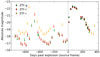 |
Fig. 25. ZTF forced-photometry light curve for SN 2020qlb binned in 30-day-long bins. We did not detect any precursor outbursts and here show the 5σ upper limits on pre-explosion outbursts. In the g- and r-bands, we typically obtain limiting magnitudes of −18 assuming that the outburst lasts for at least one month. |
As discussed in Sect. 10.2.3, most CSM-interacting SNe have strong and narrow emission lines as encountered in the spectra of H-rich type IIn. No such spectral emission lines are seen herein for SN 2020qlb or for the bump phases of many other SLSNe-I (Nicholl 2021). A possible explanation might be the overwhelming luminosity of a SLSN near its peak compared to the weak emission luminosity of low masses of expanding PPI ejected shells of CSM. In addition, if the PPI ejecta have velocities of up to 4000 km s−1 the emission lines would not be narrow.
Hosseinzadeh et al. (2022) estimate the typical mass of a CSM shell to be only 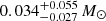 in order to power a bump. In contrast, a CSM powered SN would require a higher mass of CSM to interact with the SN ejecta which, in turn, could generate the characteristic strong and narrow emission lines. Liu et al. (2018, Table 1) when modeling the complete light curves of SLSNe iPTF15esb and iPTF13dcc with only CSM interaction required a total of
  and
and  to successfully model the two light curves. The lower CSM masses required to power a bump would therefore emit much weaker narrow emission lines, and presumably not be observed, than would the significantly higher CSM masses required to power an entire SLSN light curve.
External CSM density fluctuations could conceivably be caused by other pre-SN processes. One possible mechanism, known as wave-driven mass loss (Quataert & Shiode 2012; Shiode & Quataert 2014), involves super-Eddington fusion in the post-carbon burning phase, which could generate convection that could create acoustic waves capable of unbinding several solar masses of the stellar envelope in the last months or years prior to the SN explosion.
An additional possible source of CSM density fluctuations might be the interaction of a SN progenitor star’s binary companion with an otherwise smooth CSM. Schwarz & Pringle (1996) modeled the undulations in the radio light curve of SN 1979C (Weiler et al. 1992) by a companion star’s periastron passage using hydrodynamical simulations to determine that pronounced and asymmetrical spiral patterns in a massive (red supergiant) star’s CSM can be formed. They also point out that a low viewing angle to the binary’s orbital plane is important to observe the effects of the density variations. Ryder et al. (2004) discuss this mechanism as a possible explanation to modulations in the Type II SN 2001ig radio band light curves. Morris et al. (2006) and Mauron & Huggins (2006) discuss the Hubble Space Telescope (HST) image of LL Pegasi (AFGL 3068 or IRAS 23166+1655) as showing nested spiral shells of CSM predicted to occur when a mass losing star has a binary companion. Maercker et al. (2012) found a similar spiral pattern of CSM around R Sculptoris when using the Atacama Large Millimeter/submillimeter Array (ALMA). Others (e.g., Fraser et al. 2013) mention this mechanism as a possible source of variable CSM interaction. This hypothesis is compelling as it could recreate the oscillatory form of the light curve residuals. However, the eventual robustness in the likelihood of its occurrence requires further statistical study.
The inspiral of a compact object (neutron star or a black hole) into the helium core of a massive binary companion star, which could expel stellar material in the form of a slowly expanding, dense and toroidally formed CSM prior to triggering conditions for a SN explosion, has been discussed by (e.g., Chevalier 2012) and modeled by Schrøder et al. (2020). This type of merger-driven explosion provides a natural mechanism capable of creating aspherical CSM that could produce undulations in SLSNe-I light curves. Future efforts using multidimensional analysis of the explosion mechanisms and their resulting light curves are required to add credence to this compelling scenario.
The more general hypothesis of ejecta interaction with density fluctuations in the CSM as the undulation source must therefore be retained. As discussed, several differing processes could give rise to the required CSM density variations.
10.3.4. Breakdown of assumptions
The idea that assumptions of simplified light curve models might break down already by the time of the SLSN peak luminosity or even earlier could conceivably explain unexpected phenomena. It is also possible to consider increased model intricacies to achieve the same end.
Kaplan & Soker (2020) discuss how the sudden light curve drop observed in SN 2018don could be modeled by jets driving the ejecta at the poles faster than at the equatorial regions. This scenario is expected to result in a strong initial light curve phase followed by an abrupt drop when the expansion eventually engulfs the asymmetry. The expectation here would be to find early time divergences from SN light curves otherwise unaffected by jets.
Spectropolarimetry has been used as a measure of the asymmetry of a SN which might be caused by, for example, failed jets or an asymmetric CSM (Nicholl 2021; Wang & Wheeler 2008). Since magnetars have been suggested as gamma-ray burst (GRB) power sources, they could thereby launch jets, which if failed, could easily cause inner asphericities in the ejecta. For instance, Inserra et al. (2016) found that SLSN-I SN 2015bn showed significant polarization 24 days before and 27 days after maximum brightness, where the latter phase had a higher polarization. In addition, Saito et al. (2020) found that superluminous SN 2017egm had higher polarization at late times. Both studies concluded that the inner ejecta were more aspherical than the outer ejecta. However, several other SLSNe have had detections consistent with zero polarization and thus have a spherical ejecta (e.g., Leloudas et al. 2015; Cikota et al. 2018; Lee 2019, 2020; Poidevin et al. 2022), implying that significant asymmetries may only appear in a minority of SLSNe.
Vurm & Metzger (2021) relaxed the assumption that a magnetar’s power output is 100% thermalized by the SLSN ejecta. Three dimensional simulations tracking the coupled evolutions of electron/positron pairs as well as photons in both the ejecta and the nebula were used to create a detailed model for the thermalization and escape of high energy radiation from the SN. The additional consideration of additional parameters and processes affecting gamma leakage and the effective opacity (normally assumed constant) could both put constraints on the magnetar parameters and add model flexibility.
Undulations could conceivably be caused by a geometric asymmetry of the ejecta. Spherical asymmetry could allow successive break-outs of hotter ejecta thereby brightening the light curve. For instance, the development of multi-dimensional hydrodynamical instabilities might create pockets wherein the effective diffusion time would be reduced, enabling energy from the central engine to flow relatively unimpeded through the ejecta brightening the light curve. Alternatively, successive blockages of brighter areas by regions of optically thick material could conceivably cause reductions in the SN’s light curve. The continued use of 2D and 3D simulations which can reproduce anisotropies and hydrodynamical instabilities to more properly model the light curves of magnetar-powered SLSNe, for example as done by Chen et al. (2016), Suzuki & Maeda (2017, 2021), (2D); Suzuki & Maeda (2019), Chen et al. (2020), (3D); and Blondin & Chevalier (2017), (2D and 3D), might bring clarity to this possibility.
11. Conclusions
SN 2020qlb is an extensively sampled SLSN-I that is among the most luminous (peak Mg = −22.25 mag) and long-rising (72.4 days from 10% of maximum) SNe currently known. We estimate the total radiated energy of SN 2002qlb to have been ≳2.8 ± 0.3 × 1051 erg. It exploded in a low-mass (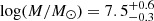 ), low-metallicity (12 + log(O/H)=8.0 ± 0.2 dex, direct method) galaxy.
A large photometric data set is available and characterized by an excellent temporal coverage, even during the near peak solar conjunction by Swift, broad wavelength coverage by the 14 measurement bands employed, and with a high measurement cadence by the ZTF survey telescope. We herein construct the SN 2020qlb bolometric light curve, estimate the photospheric radius and temperature evolutions, and fit power source models to the resulting data.
We consider and rule out a 56Ni decay power source model due to unphysical parameter results. We disfavor the CSM power source model due to – amongst other things – the lack of the signature spectroscopic features of CSM interaction. We favor a model wherein the dipole spindown energy deposition of a rapidly rotating magnetar can power SN 2020qlb’s light curve. The magnetar model, using physically reasonable parameter values, results in a close fit to the majority of the bolometric and multi-band light curves.
During the first 150 days, the magnetar model residual has two to three oscillations with a 32±6 day timescale and an amplitude of about 6% of peak luminosity. Intriguingly, Nicholl (2018) found a similar magnetar residual for the well-sampled SN 2015bn where the near peak oscillatory form had a timescale of 30−50 days and an 11% amplitude.
We discuss three categories of hypotheses for the mechanism(s) behind the undulating magnetar residuals. A simple timescale argument rules out that a centrally sourced 32 day undulation could possibly survive the diffusion process as it passes through an ejecta with an 86 day diffusion timescale. In a second category, processes involving the ejecta are disfavored as they either predict a single bump or result in an unobserved wavelength dependence. We favor a third category, an external undulation source, which is the interaction of the SN ejecta with CSM density variations. Possible sources of the CSM density variations include pulsational pair instability, eruptive mass loss, the periastron passage of a companion star through an otherwise smooth CSM, and the common envelope evolution of a stellar merger-driven explosion. We also discuss whether possible breakdowns of model assumptions might result in light curve residuals.
To continue the research about the true source(s) of SLSNe undulations, we will need improved data breadth and resolution over time. An important upcoming project is the Vera Rubin Observatory’s Legacy Survey of Space and Time (LSST) which is estimated to be able to discover ∼104 SLSNe per year with more than ten data points at redshifts up to z ≲ 3 (Villar et al. 2018). Progress in modeling, data reduction and theory, large high cadence surveys such as ZTF, complemented by the depth of the LSST, should be capable of improving our understanding of the apparent SLSN undulations.
Using the criteria described in Sect. 4.2 of https://web.ipac.caltech.edu/staff/fmasci/ztf/extended_cautionary_notes.pdf
Acknowledgments
The authors would like to give special thanks to Matt Nicholl (Birmingham Univ.) for his helpful discussions regarding an early version of this work. Some of the data presented herein were obtained at the W.M. Keck Observatory, which is operated as a scientific partnership among the California Institute of Technology, the University of California and the National Aeronautics and Space Administration. The Observatory was made possible by the generous financial support of the W.M. Keck Foundation. Based on observations obtained with the Samuel Oschin Telescope 48-inch and the 60-inch Telescope at the Palomar Observatory as part of the Zwicky Transient Facility project. Z.T.F. is supported by the National Science Foundation under Grants No. AST-1440341 and AST-2034437 and a collaboration including current partners Caltech, IPAC, the Weizmann Institute for Science, the Oskar Klein Center at Stockholm University, the University of Maryland, Deutsches Elektronen-Synchrotron and Humboldt University, the TANGO Consortium of Taiwan, the University of Wisconsin at Milwaukee, Trinity College Dublin, Lawrence Livermore National Laboratories, IN2P3, University of Warwick, Ruhr University Bochum, Northwestern University and former partners the University of Washington, Los Alamos National Laboratories, and Lawrence Berkeley National Laboratories. Operations are conducted by COO, IPAC, and UW. The ZTF forced-photometry service was funded under the Heising-Simons Foundation grant nr. 12540303 (PI: Graham). SED Machine is based upon work supported by the National Science Foundation under Grant No. 1106171. The Liverpool Telescope is operated on the island of La Palma by Liverpool John Moores University in the Spanish Observatorio del Roque de los Muchachos of the Instituto de Astrofisica de Canarias with financial support from the UK Science and Technology Facilities Council. This work has been supported by the research project grant “Understanding the Dynamic Universe” funded by the Knut and Alice Wallenberg Foundation under Dnr KAW 2018.0067, and the G.R.E.A.T. research environment, funded by Vetenskapsrådet, the Swedish Research Council, project number 2016-06012. Based on observations made with the Nordic Optical Telescope, owned in collaboration by the University of Turku and Aarhus University, and operated jointly by Aarhus University, the University of Turku and the University of Oslo, representing Denmark, Finland and Norway, the University of Iceland and Stockholm University at the Observatorio del Roque de los Muchachos, La Palma, Spain, of the Instituto de Astrofisica de Canarias. The data presented here were obtained in part with ALFOSC, which is provided by the Instituto de Astrofisica de Andalucia (IAA) under a joint agreement with the University of Copenhagen and NOT. This research is partially based on observations made with the NASA/ESA Hubble Space Telescope obtained from the Space Telescope Science Institute, which is operated by the Association of Universities for Research in Astronomy, Inc., under NASA contract NAS 5-26555. These observations are associated with program SNAP-16657 (PI: Fremling). This research has made use of the SVO Filter Profile Service (http://svo2.cab.inta-csic.es/theory/fps/) supported from the Spanish MINECO through grant AYA2017-84089. T.-W.C. acknowledges the EU Funding under Marie Skłodowska-Curie grant H2020-MSCA-IF-2018-842471. Steve Schulze acknowledges support from the G.R.E.A.T. research environment, funded by Vetenskapsrådet, the Swedish Research Council, project number 2016-06012. N.L.S. is funded by the Deutsche Forschungsgemeinschaft (DFG, German Research Foundation) via the Walter Benjamin program – 461903330.
References
- Ahn, C. P., Alexandroff, R., Allende Prieto, C., et al. 2012, ApJS, 203, 21 [Google Scholar]
- Ambikasaran, S., Foreman-Mackey, D., Greengard, L., Hogg, D. W., & O’Neil, M. 2015, IEEE Trans. Pattern Anal. Mach. Intell., 38, 252 [Google Scholar]
- Angus, C. R., Smith, M., Sullivan, M., et al. 2019, MNRAS, 487, 2215 [NASA ADS] [CrossRef] [Google Scholar]
- Arnett, W. D. 1982, ApJ, 253, 785 [Google Scholar]
- Asplund, M., Grevesse, N., Sauval, A. J., & Scott, P. 2009, ARA&A, 47, 481 [NASA ADS] [CrossRef] [Google Scholar]
- Bellm, E. C., & Sesar, B. 2016, Astrophysics Source Code Library [record ascl:1602.002] [Google Scholar]
- Bellm, E. C., Kulkarni, S. R., Graham, M. J., et al. 2019, PASP, 131, 018002 [Google Scholar]
- Bhirombhakdi, K., Chornock, R., Miller, A. A., et al. 2019, MNRAS, 488, 3783 [NASA ADS] [CrossRef] [Google Scholar]
- Blagorodnova, N., Neill, J. D., Walters, R., et al. 2018, PASP, 130, 035003 [Google Scholar]
- Blondin, J. M., & Chevalier, R. A. 2017, ApJ, 845, 139 [NASA ADS] [CrossRef] [Google Scholar]
- Breeveld, A. A., Landsman, W., Holland, S. T., et al. 2011, AIP Conf. Ser., 1358, 373 [Google Scholar]
- Burrows, D. N., Hill, J. E., Nousek, J. A., et al. 2005, Space Sci. Rev., 120, 165 [Google Scholar]
- Byler, N., Dalcanton, J. J., Conroy, C., & Johnson, B. D. 2017, ApJ, 840, 44 [Google Scholar]
- Calzetti, D., Armus, L., Bohlin, R. C., et al. 2000, ApJ, 533, 682 [NASA ADS] [CrossRef] [Google Scholar]
- Campbell, A., Terlevich, R., & Melnick, J. 1986, MNRAS, 223, 811 [NASA ADS] [CrossRef] [Google Scholar]
- Cano, Z., Izzo, L., de Ugarte Postigo, A., et al. 2017, A&A, 605, A107 [NASA ADS] [CrossRef] [EDP Sciences] [Google Scholar]
- Chabrier, G. 2003, PASP, 115, 763 [Google Scholar]
- Chambers, K. C., Magnier, E. A., Metcalfe, N., et al. 2016, ArXiv e-prints [arXiv:1612.05560] [Google Scholar]
- Chandra, P. 2018, Space Sci. Rev., 214, 27 [NASA ADS] [CrossRef] [Google Scholar]
- Chandra, P., Chevalier, R. A., Chugai, N., Fransson, C., & Soderberg, A. M. 2015, ApJ, 810, 32 [NASA ADS] [CrossRef] [Google Scholar]
- Chatzopoulos, E., Wheeler, J. C., & Vinko, J. 2012, ApJ, 746, 121 [Google Scholar]
- Chatzopoulos, E., Wheeler, J. C., Vinko, J., Horvath, Z. L., & Nagy, A. 2013, ApJ, 773, 76 [NASA ADS] [CrossRef] [Google Scholar]
- Chen, K.-J. 2021, Int. J. Mod. Phys. D, 30, 2130001 [NASA ADS] [CrossRef] [Google Scholar]
- Chen, K.-J., Woosley, S. E., & Sukhbold, T. 2016, ApJ, 832, 73 [NASA ADS] [CrossRef] [Google Scholar]
- Chen, T.-W., Smartt, S. J., Yates, R. M., et al. 2017, MNRAS, 470, 3566 [NASA ADS] [CrossRef] [Google Scholar]
- Chen, T. W., Inserra, C., Fraser, M., et al. 2018, ApJ, 867, L31 [NASA ADS] [CrossRef] [Google Scholar]
- Chen, K.-J., Woosley, S. E., & Whalen, D. J. 2020, ApJ, 893, 99 [NASA ADS] [CrossRef] [Google Scholar]
- Chen, Z. H., Yan, L., Kangas, T., et al. 2022a, ApJ, submitted [arXiv:2202.02060] [Google Scholar]
- Chen, Z. H., Yan, L., Kangas, T., et al. 2022b, ApJ, submitted [arXiv:2202.02059] [Google Scholar]
- Chevalier, R. A. 2012, ApJ, 752, L2 [NASA ADS] [CrossRef] [Google Scholar]
- Chugai, N. N., & Utrobin, V. P. 2022, MNRAS, 512, L71 [NASA ADS] [CrossRef] [Google Scholar]
- Cikota, A., Leloudas, G., Bulla, M., et al. 2018, MNRAS, 479, 4984 [NASA ADS] [CrossRef] [Google Scholar]
- Clocchiatti, A., & Wheeler, J. C. 1997, ApJ, 491, 375 [Google Scholar]
- Conroy, C., Gunn, J. E., & White, M. 2009, ApJ, 699, 486 [Google Scholar]
- Coppejans, D. L., Matthews, D., Margutti, R., et al. 2021a, ATel, 14393, 1 [NASA ADS] [Google Scholar]
- Coppejans, D. L., Matthews, D., Margutti, R., et al. 2021b, ATel, 14418, 1 [NASA ADS] [Google Scholar]
- De Cia, A., Gal-Yam, A., Rubin, A., et al. 2018, ApJ, 860, 100 [NASA ADS] [CrossRef] [Google Scholar]
- Dekany, R., Smith, R. M., Riddle, R., et al. 2020, PASP, 132, 038001 [NASA ADS] [CrossRef] [Google Scholar]
- Denissenya, M., Grossan, B., & Linder, E. V. 2021, Phys. Rev. D, 104, 023007 [NASA ADS] [CrossRef] [Google Scholar]
- Dey, A., Schlegel, D. J., Lang, D., et al. 2019, AJ, 157, 168 [Google Scholar]
- Eftekhari, T., Berger, E., Margalit, B., et al. 2019, ApJ, 876, L10 [NASA ADS] [CrossRef] [Google Scholar]
- Eftekhari, T., Margalit, B., Omand, C. M. B., et al. 2021, ApJ, 912, 21 [NASA ADS] [CrossRef] [Google Scholar]
- Evans, P. A., Beardmore, A. P., Page, K. L., et al. 2007, A&A, 469, 379 [NASA ADS] [CrossRef] [EDP Sciences] [Google Scholar]
- Evans, P. A., Beardmore, A. P., Page, K. L., et al. 2009, MNRAS, 397, 1177 [Google Scholar]
- Fitzpatrick, E. L. 1999, PASP, 111, 63 [Google Scholar]
- Foreman-Mackey, D., Sick, J., & Johnson, B. 2014, https://doi.org/10.5281/zenodo.12157 [Google Scholar]
- Fransson, C., Benvenuti, P., Gordon, C., et al. 1984, A&A, 132, 1 [NASA ADS] [Google Scholar]
- Fraser, M., Inserra, C., Jerkstrand, A., et al. 2013, MNRAS, 433, 1312 [NASA ADS] [CrossRef] [Google Scholar]
- Gal-Yam, A. 2012, Science, 337, 927 [Google Scholar]
- Gal-Yam, A. 2019, ARA&A, 57, 305 [Google Scholar]
- Gal-Yam, A., Mazzali, P., Ofek, E. O., et al. 2009, Nature, 462, 624 [NASA ADS] [CrossRef] [Google Scholar]
- Graham, M. J., Kulkarni, S. R., Bellm, E. C., et al. 2019, PASP, 131, 078001 [Google Scholar]
- Guillochon, J., Nicholl, M., Villar, V. A., et al. 2018, ApJS, 236, 6 [NASA ADS] [CrossRef] [Google Scholar]
- Hatsukade, B., Tominaga, N., Morokuma, T., et al. 2021, ApJ, 911, L1 [NASA ADS] [CrossRef] [Google Scholar]
- Heger, A., & Woosley, S. E. 2002, ApJ, 567, 532 [Google Scholar]
- HI4PI Collaboration (Ben Bekhti, N., et al.) 2016, A&A, 594, A116 [NASA ADS] [CrossRef] [EDP Sciences] [Google Scholar]
- Hogg, D. W., Baldry, I. K., Blanton, M. R., & Eisenstein, D. J. 2002, ArXiv e-prints [arXiv:astro-ph/0210394] [Google Scholar]
- Hosseinzadeh, G., Berger, E., Metzger, B. D., et al. 2022, ApJ, 933, 14 [NASA ADS] [CrossRef] [Google Scholar]
- Howell, D. A. 2017, in Superluminous Supernovae, eds. A. W. Alsabti, & P. Murdin (Cham: Springer International Publishing), 1 [Google Scholar]
- Inserra, C., Smartt, S. J., Jerkstrand, A., et al. 2013, ApJ, 770, 128 [NASA ADS] [CrossRef] [Google Scholar]
- Inserra, C., Bulla, M., Sim, S. A., & Smartt, S. J. 2016, ApJ, 831, 79 [NASA ADS] [CrossRef] [Google Scholar]
- Inserra, C., Nicholl, M., Chen, T. W., et al. 2017, MNRAS, 468, 4642 [NASA ADS] [CrossRef] [Google Scholar]
- Inserra, C., Smartt, S. J., Gall, E. E. E., et al. 2018, MNRAS, 475, 1046 [NASA ADS] [CrossRef] [Google Scholar]
- Janka, H.-T. 2012, Annu. Rev. Nucl. Part. Sci., 62, 407 [NASA ADS] [CrossRef] [Google Scholar]
- Jiang, B., Jiang, S., & Ashley Villar, V. 2020, Res. Notes Am. Astron. Soc., 4, 16 [Google Scholar]
- Kaplan, N., & Soker, N. 2020, MNRAS, 494, 5909 [NASA ADS] [CrossRef] [Google Scholar]
- Kasen, D. 2017, in Unusual Supernovae and Alternative Power Sources, eds. A. W. Alsabti, & P. Murdin (Cham: Springer International Publishing), 1 [Google Scholar]
- Kasen, D., & Bildsten, L. 2010, ApJ, 717, 245 [NASA ADS] [CrossRef] [Google Scholar]
- Kasen, D., Woosley, S. E., & Heger, A. 2011, ApJ, 734, 102 [NASA ADS] [CrossRef] [Google Scholar]
- Kashiyama, K., Murase, K., Bartos, I., Kiuchi, K., & Margutti, R. 2016, ApJ, 818, 94 [NASA ADS] [CrossRef] [Google Scholar]
- Katsuda, S., Maeda, K., Bamba, A., et al. 2016, ApJ, 832, 194 [NASA ADS] [CrossRef] [Google Scholar]
- Kennicutt, R. C., Jr. 1998, ARA&A, 36, 189 [Google Scholar]
- Komatsu, E., Smith, K. M., Dunkley, J., et al. 2011, ApJS, 192, 18 [Google Scholar]
- Law, C. J., Omand, C. M. B., Kashiyama, K., et al. 2019, ApJ, 886, 24 [NASA ADS] [CrossRef] [Google Scholar]
- Lee, C.-H. 2019, ApJ, 875, 121 [NASA ADS] [CrossRef] [Google Scholar]
- Lee, C.-H. 2020, Astron. Nachr., 341, 651 [NASA ADS] [CrossRef] [Google Scholar]
- Leja, J., Johnson, B. D., Conroy, C., van Dokkum, P. G., & Byler, N. 2017, ApJ, 837, 170 [NASA ADS] [CrossRef] [Google Scholar]
- Leloudas, G., Patat, F., Maund, J. R., et al. 2015, ApJ, 815, L10 [NASA ADS] [CrossRef] [Google Scholar]
- Liu, L.-D., Wang, L.-J., Wang, S.-Q., & Dai, Z.-G. 2018, ApJ, 856, 59 [NASA ADS] [CrossRef] [Google Scholar]
- Lunnan, R., Chornock, R., Berger, E., et al. 2014, ApJ, 787, 138 [NASA ADS] [CrossRef] [Google Scholar]
- Lunnan, R., Chornock, R., Berger, E., et al. 2015, ApJ, 804, 90 [NASA ADS] [CrossRef] [Google Scholar]
- Lunnan, R., Fransson, C., Vreeswijk, P. M., et al. 2018, Nat. Astron., 2, 887 [NASA ADS] [CrossRef] [Google Scholar]
- Lupton, R., Blanton, M. R., Fekete, G., et al. 2004, PASP, 116, 133 [NASA ADS] [CrossRef] [Google Scholar]
- Luridiana, V., Morisset, C., & Shaw, R. A. 2013, Astrophysics Source Code Library [record ascl:1304.021] [Google Scholar]
- Lyman, J. D., Bersier, D., & James, P. A. 2014, MNRAS, 437, 3848 [Google Scholar]
- Maercker, M., Mohamed, S., Vlemmings, W. H. T., et al. 2012, Nature, 490, 232 [NASA ADS] [CrossRef] [Google Scholar]
- Mamajek, E. E., Torres, G., Prsa, A., et al. 2015, ArXiv e-prints [arXiv:1510.06262] [Google Scholar]
- Masci, F. J., Laher, R. R., Rusholme, B., et al. 2019, PASP, 131, 018003 [Google Scholar]
- Mauron, N., & Huggins, P. J. 2006, A&A, 452, 257 [NASA ADS] [CrossRef] [EDP Sciences] [Google Scholar]
- Metzger, B. D., Vurm, I., Hascoët, R., & Beloborodov, A. M. 2014, MNRAS, 437, 703 [NASA ADS] [CrossRef] [Google Scholar]
- Metzger, B. D., Beniamini, P., & Giannios, D. 2018, ApJ, 857, 95 [NASA ADS] [CrossRef] [Google Scholar]
- Miller, A. A., Yao, Y., Bulla, M., et al. 2020, ApJ, 902, 47 [NASA ADS] [CrossRef] [Google Scholar]
- Mondal, S., Bera, A., Chandra, P., & Das, B. 2020, MNRAS, 498, 3863 [NASA ADS] [CrossRef] [Google Scholar]
- Moriya, T. J., Blinnikov, S. I., Tominaga, N., et al. 2013, MNRAS, 428, 1020 [NASA ADS] [CrossRef] [Google Scholar]
- Moriya, T. J., Sorokina, E. I., & Chevalier, R. A. 2018, Space Sci. Rev., 214, 59 [Google Scholar]
- Moriya, T. J., Murase, K., Kashiyama, K., & Blinnikov, S. I. 2022, MNRAS, 513, 6210 [NASA ADS] [CrossRef] [Google Scholar]
- Morris, M., Sahai, R., Matthews, K., et al. 2006, IAU Symp., 234, 469 [CrossRef] [Google Scholar]
- Murase, K., Kashiyama, K., Kiuchi, K., & Bartos, I. 2015, ApJ, 805, 82 [NASA ADS] [CrossRef] [Google Scholar]
- Murase, K., Kashiyama, K., & Mészáros, P. 2016, MNRAS, 461, 1498 [NASA ADS] [CrossRef] [Google Scholar]
- Murase, K., Omand, C. M. B., Coppejans, D. L., et al. 2021, MNRAS, 508, 44 [NASA ADS] [CrossRef] [Google Scholar]
- Nicholl, M. 2018, Res. Notes Am. Astron. Soc., 2, 230 [NASA ADS] [Google Scholar]
- Nicholl, M. 2021, Astron. Geophys., 62, 5.34 [NASA ADS] [CrossRef] [Google Scholar]
- Nicholl, M., Smartt, S. J., Jerkstrand, A., et al. 2013, Nature, 502, 346 [NASA ADS] [CrossRef] [Google Scholar]
- Nicholl, M., Berger, E., Smartt, S. J., et al. 2016, ApJ, 826, 39 [NASA ADS] [CrossRef] [Google Scholar]
- Nicholl, M., Guillochon, J., & Berger, E. 2017, ApJ, 850, 55 [NASA ADS] [CrossRef] [Google Scholar]
- Oke, J. B., & Gunn, J. E. 1982, PASP, 94, 586 [Google Scholar]
- Oke, J. B., & Gunn, J. E. 1983, ApJ, 266, 713 [NASA ADS] [CrossRef] [Google Scholar]
- Oke, J. B., Cohen, J. G., Carr, M., et al. 1995, PASP, 107, 375 [Google Scholar]
- Omand, C. M. B., Kashiyama, K., & Murase, K. 2018, MNRAS, 474, 573 [NASA ADS] [CrossRef] [Google Scholar]
- Ørum, S. V., Ivens, D. L., Strandberg, P., et al. 2020, A&A, 643, A47 [NASA ADS] [CrossRef] [EDP Sciences] [Google Scholar]
- Osterbrock, D. E. 1989, Astrophysics of Gaseous Nebulae and Active Galactic Nuclei (Sausalito: University Science Books) [Google Scholar]
- Perez-Fournon, I., Poidevin, F., Angel, C. J., et al. 2020, Transient Name Server Classification Report, 2020-2456, 1 [Google Scholar]
- Perley, D. A. 2019, PASP, 131, 084503 [Google Scholar]
- Perley, D. A., Quimby, R. M., Yan, L., et al. 2016, ApJ, 830, 13 [NASA ADS] [CrossRef] [Google Scholar]
- Piascik, A. S., Steele, I. A., Bates, S. D., et al. 2014, SPIE Conf. Ser., 9147, 91478H [NASA ADS] [Google Scholar]
- Poidevin, F., Omand, C. M. B., Pérez-Fournon, I., et al. 2022, MNRAS, 511, 5948 [NASA ADS] [CrossRef] [Google Scholar]
- Quataert, E., & Shiode, J. 2012, MNRAS, 423, L92 [NASA ADS] [CrossRef] [Google Scholar]
- Quimby, R. M., Aldering, G., Wheeler, J. C., et al. 2007, ApJ, 668, L99 [NASA ADS] [CrossRef] [Google Scholar]
- Quimby, R. M., De Cia, A., Gal-Yam, A., et al. 2018, ApJ, 855, 2 [Google Scholar]
- Richardson, D., Branch, D., Casebeer, D., et al. 2002, AJ, 123, 745 [NASA ADS] [CrossRef] [Google Scholar]
- Rigault, M., Neill, J. D., Blagorodnova, N., et al. 2019, A&A, 627, A115 [NASA ADS] [CrossRef] [EDP Sciences] [Google Scholar]
- Roming, P. W. A., Kennedy, T. E., Mason, K. O., et al. 2005, Space Sci. Rev., 120, 95 [Google Scholar]
- Ryder, S. D., Sadler, E. M., Subrahmanyan, R., et al. 2004, MNRAS, 349, 1093 [NASA ADS] [CrossRef] [Google Scholar]
- Saito, S., Tanaka, M., Moriya, T. J., et al. 2020, ApJ, 894, 154 [NASA ADS] [CrossRef] [Google Scholar]
- Schrøder, S. L., MacLeod, M., Loeb, A., Vigna-Gómez, A., & Mandel, I. 2020, ApJ, 892, 13 [CrossRef] [Google Scholar]
- Schulze, S., Krühler, T., Leloudas, G., et al. 2018, MNRAS, 473, 1258 [NASA ADS] [CrossRef] [Google Scholar]
- Schulze, S., Yaron, O., Sollerman, J., et al. 2021, ApJS, 255, 29 [NASA ADS] [CrossRef] [Google Scholar]
- Schwarz, D. H., & Pringle, J. E. 1996, MNRAS, 282, 1018 [NASA ADS] [CrossRef] [Google Scholar]
- Shiode, J. H., & Quataert, E. 2014, ApJ, 780, 96 [Google Scholar]
- Smith, N. 2014, ARA&A, 52, 487 [NASA ADS] [CrossRef] [Google Scholar]
- Smith, N., Li, W., Foley, R. J., et al. 2007, ApJ, 666, 1116 [NASA ADS] [CrossRef] [Google Scholar]
- Smith, N., Li, W., Silverman, J. M., Ganeshalingam, M., & Filippenko, A. V. 2011, MNRAS, 415, 773 [NASA ADS] [CrossRef] [Google Scholar]
- Sollerman, J., Leibundgut, B., & Spyromilio, J. 1998, A&A, 337, 207 [NASA ADS] [Google Scholar]
- Sorokina, E., Blinnikov, S., Nomoto, K., Quimby, R., & Tolstov, A. 2016, ApJ, 829, 17 [NASA ADS] [CrossRef] [Google Scholar]
- Steele, I. A., Smith, R. J., Rees, P. C., et al. 2004, SPIE Conf. Ser., 5489, 679 [Google Scholar]
- Strotjohann, N. L., Ofek, E. O., Gal-Yam, A., et al. 2021, ApJ, 907, 99 [NASA ADS] [CrossRef] [Google Scholar]
- Suzuki, A., & Maeda, K. 2017, MNRAS, 466, 2633 [NASA ADS] [CrossRef] [Google Scholar]
- Suzuki, A., & Maeda, K. 2019, ApJ, 880, 150 [NASA ADS] [CrossRef] [Google Scholar]
- Suzuki, A., & Maeda, K. 2021, ApJ, 908, 217 [NASA ADS] [CrossRef] [Google Scholar]
- Taddia, F., Sollerman, J., Fremling, C., et al. 2019, A&A, 621, A71 [NASA ADS] [CrossRef] [EDP Sciences] [Google Scholar]
- Tanaka, S. J., & Takahara, F. 2010, ApJ, 715, 1248 [NASA ADS] [CrossRef] [Google Scholar]
- Tanaka, S. J., & Takahara, F. 2013, MNRAS, 429, 2945 [CrossRef] [Google Scholar]
- Villar, V. A., Berger, E., Metzger, B. D., & Guillochon, J. 2017, ApJ, 849, 70 [NASA ADS] [CrossRef] [Google Scholar]
- Villar, V. A., Nicholl, M., & Berger, E. 2018, ApJ, 869, 166 [NASA ADS] [CrossRef] [Google Scholar]
- Vurm, I., & Metzger, B. D. 2021, ApJ, 917, 77 [NASA ADS] [CrossRef] [Google Scholar]
- Wang, L., & Wheeler, J. C. 2008, ARA&A, 46, 433 [Google Scholar]
- Weiler, K. W., van Dyk, S. D., Pringle, J. E., & Panagia, N. 1992, ApJ, 399, 672 [NASA ADS] [CrossRef] [Google Scholar]
- Wheeler, J. C., Chatzopoulos, E., Vinkó, J., & Tuminello, R. 2017, ApJ, 851, L14 [NASA ADS] [CrossRef] [Google Scholar]
- Woosley, S. E. 2010, ApJ, 719, L204 [NASA ADS] [CrossRef] [Google Scholar]
- Woosley, S. E. 2017, ApJ, 836, 244 [Google Scholar]
- Wright, A. H., Robotham, A. S. G., Bourne, N., et al. 2016, MNRAS, 460, 765 [Google Scholar]
- Yan, L., Lunnan, R., Perley, D. A., et al. 2017a, ApJ, 848, 6 [NASA ADS] [CrossRef] [Google Scholar]
- Yan, L., Quimby, R., Gal-Yam, A., et al. 2017b, ApJ, 840, 57 [NASA ADS] [CrossRef] [Google Scholar]
- Yao, Y., Miller, A. A., Kulkarni, S. R., et al. 2019, ApJ, 886, 152 [NASA ADS] [CrossRef] [Google Scholar]
- Yoshida, T., Umeda, H., Maeda, K., & Ishii, T. 2016, MNRAS, 457, 351 [Google Scholar]
- Zackay, B., Ofek, E. O., & Gal-Yam, A. 2016, ApJ, 830, 27 [NASA ADS] [CrossRef] [Google Scholar]
All Tables
Comparison of two methods for magnetar modeling and their best fit (median and 1σ) parameters.
All Figures
|
Fig. 1. Left: pre-SN image retrieved from the Dark Energy Camera Legacy Surveys (DR9). Right: image of SN 2020qlb taken on August 9, 2020 (61 rest frame days before peak) with the Liverpool Telescope in ugriz frames and stacked (Lupton et al. 2004) around the SN location. Each image is 45 by 45 arcsec. |
| In the text | |
|
Fig. 2. Absolute magnitude (rest frame) light curves from ∼1800 to 18500 Å, including the Liverpool Telescope SDSS filters as triangles, the Swift UVOT filters as squares and the ZTF filters as circles. The black triangles at the top indicate the phases of available spectra. Phase = 0 (at peak ZTF g-band) is estimated in Sect. 3.2. The light curves in the different bands were shifted for illustration purposes. |
| In the text | |
|
Fig. 3. Spectral sequence of SN 2020qlb. The dark blue SN 2020qlb spectra were smoothed using a Savitzky-Golay low pass filter. A lighter shade of blue is used for un-smoothed data and measurement errors. Spectra from a well studied SLSN-I (SN 2015bn) are shown in gray for comparison. P-Cygni profile minima used for velocity estimations are marked in dark red. Narrow host galaxy emission lines ([O III], Hα and [O II]) used for redshift estimation are indicated with green, red and blue vertical dashed lines. Blended Fe II absorption features, as well as [Mg I] and [Ca II] emission features are noted in black. Nebular phase [O I] and [O II] broad emission lines are noted in green. |
| In the text | |
|
Fig. 4. ZTF r- and g-band flux in the observer frame near in time to the initial detection of SN 2020qlb. Points used for the second degree polynomial fits are darkened. |
| In the text | |
|
Fig. 5. GP interpolated ZTF-g and -r (rest frame) light curves. Horizontal lines used to calculate the different rise and decline times are plotted in gray. The ballooning effect of the GP interpolation algorithm is clearly seen in the solar conjunction gap in the data between 120 and 170 days past explosion. |
| In the text | |
|
Fig. 6. Peak Mg versus e-folding rise time for 69 ZTF SLSNe-I from Chen et al. (2022b) are compared with SN 2020qlb. |
| In the text | |
|
Fig. 7. SN 2020qlb g − r color evolution created from the ZTF-g and -r filter GP interpolations in Sect. 3.2 in blue and the g − r measurements with the LT in red. The gray background is a scatter plot of the 75 SLSNe-I and orange is for the 9 with 0.13 < z < 0.19 from Chen et al. (2022b, Fig. 13). |
| In the text | |
|
Fig. 8. Example (phase −51.2 days) of how a blackbody fit to photometric data is used to estimate the temperature and photospheric radius. The three UVOT UV filter measurements are excluded due to the UV line-blanketing effect. |
| In the text | |
|
Fig. 9. Rest frame radius evolution of the SN photosphere from blackbody fits to data from UVOT epochs. A fourth degree polynomial was fit to the data. SLSN-I radius evolutions from Chen et al. (2022b) are shown in gray. |
| In the text | |
|
Fig. 10. Velocity evolution of the SN photosphere shown in green based on the fourth degree polynomial fit to the photosphere radius evolution shown in Fig. 9. P-Cygni absorption line velocity estimates from Sect. 4.3 are included as well. |
| In the text | |
|
Fig. 11. Temperature evolution of the SN 2020qlb photosphere (blue: fit to UVOT + optical data; orange: fit to LT ugriz data; red: fit to spectra) in comparison to the 31 SLSN-I temperature evolutions from Chen et al. (2022b) shown in light gray. |
| In the text | |
|
Fig. 12. Example, at a phase of −51.2 days, of how an SED is constructed using linear interpolations between photometric data points and extrapolated on both ends as explained in the text. |
| In the text | |
|
Fig. 13. Interpolated bolometric luminosities are shown interlaced with the bolometric luminosities estimated in Sect. 6.2. |
| In the text | |
|
Fig. 14. Bolometric correction as a function of rest frame g − r color. A second degree polynomial curve-fit is compared to the post peak bolometric correction to the g-band (BCg) versus (g − r) color data. The data are shown connected in time sequence. The first seven points were removed from the curve-fit. |
| In the text | |
|
Fig. 15. Bolometric light curve plotted together with the best-fit magnetar and Arnett radioactive source models. Forcing the 56Ni mass to be less than or equal to the ejecta mass results in the red dashdot line. |
| In the text | |
|
Fig. 16. Multi-band light curve of SN 2020qlb inferred from the magnetar-model, with bands offset for clarity. The colored lines show the range of most likely models generated by MOSFiT. Phase = 0 is where the ZTF g-band is maximized in the observer frame (MJD 59140.0). |
| In the text | |
|
Fig. 17. 1D and 2D posterior distributions of the magnetar model parameters from the MOSFiT model. Median and 1σ values are marked and labeled. These are used as the best fit values. |
| In the text | |
|
Fig. 18. Predicted radio emission for SN 2020qlb at 3 (red), 15 (green), and 100 (blue) GHz. The dashed and solid lines represent estimates of free-free absorption using an un-ionized and singly ionized oxygen ejecta, respectively. |
| In the text | |
|
Fig. 19. Light curve residuals after subtracting a polynomial (order indicated in each panel) to the first 200 days of data. Visual inspection indicates fluctuations with an approximate timescale of ∼30 days in all filters; this is indicated in each subplot with an arrow showing time between peaks/troughs. |
| In the text | |
|
Fig. 20. Bolometric light curve less magnetar residual and the GP interpolation of the residual, both normalized by the maximum magnetar model luminosity. The phase of the magnetar model maximum (−19.4 days) is marked with a vertical line for reference. |
| In the text | |
|
Fig. 21. Fast Fourier transform of the GP interpolation of the bolometric LC less magnetar model residual for phases up to +60 days as shown in darker blue in Fig. 20. |
| In the text | |
|
Fig. 22. HST image of the host galaxy of SN 2020qlb, corresponding to a rest-frame wavelength of 2900 Å, and taken at a phase of +386 days past the g-band peak. The host galaxy appears to have two knots of emission, with the supernova located at the northern knot. The apparent point source could include supernova emission, or be a star-forming region in the host galaxy; a template image would be needed to tell the two apart. The source visible in the bottom left of the image is caused by a cosmic ray. |
| In the text | |
|
Fig. 23. Spectral energy distribution (SED) of the SN 2020qlb host galaxy from 1000 to 60 000 Å (black data points, Table 3). The solid line displays the best-fitting model of the SED. The red squares represent the model-predicted magnitudes. The fitting parameters are shown in the upper-left corner. The abbreviation “n.o.f.” stands for numbers of filters. |
| In the text | |
|
Fig. 24. T4 third degree polynomial residual relative to the zero phase T4 in red at Swift phases and in orange at LT phases. |
| In the text | |
|
Fig. 25. ZTF forced-photometry light curve for SN 2020qlb binned in 30-day-long bins. We did not detect any precursor outbursts and here show the 5σ upper limits on pre-explosion outbursts. In the g- and r-bands, we typically obtain limiting magnitudes of −18 assuming that the outburst lasts for at least one month. |
| In the text | |
Current usage metrics show cumulative count of Article Views (full-text article views including HTML views, PDF and ePub downloads, according to the available data) and Abstracts Views on Vision4Press platform.
Data correspond to usage on the plateform after 2015. The current usage metrics is available 48-96 hours after online publication and is updated daily on week days.
Initial download of the metrics may take a while.