| Issue |
A&A
Volume 679, November 2023
|
|
|---|---|---|
| Article Number | A125 | |
| Number of page(s) | 15 | |
| Section | Cosmology (including clusters of galaxies) | |
| DOI | https://doi.org/10.1051/0004-6361/202346495 | |
| Published online | 29 November 2023 | |
Reionisation time field reconstruction from 21 cm signal maps
Université de Strasbourg, CNRS UMR 7550, Observatoire Astronomique de Strasbourg, Strasbourg, France
e-mail: This email address is being protected from spambots. You need JavaScript enabled to view it.
Received:
24
March
2023
Accepted:
8
September
2023
Abstract
Context. During the epoch of reionisation, the intergalactic medium is reionised by the UV radiation from the first generation of stars and galaxies. One tracer of the process is the 21 cm line of hydrogen that will be observed by the Square Kilometre Array (SKA) at low frequencies, thus imaging the distribution of ionised and neutral regions and their evolution.
Aims. To prepare for these upcoming observations, we investigate a deep learning method to predict from 21 cm maps the reionisation time field (treion(r)), the time at which each location has been reionised. The treion(r) method encodes the propagation of ionisation fronts in a single field, and gives access to times of local reionisation or to the extent of the radiative reach of early sources. Moreover it gives access to the time evolution of ionisation on the plane of sky, when this evolution is usually probed along the line-of-sight direction.
Methods. We trained a convolutional neural network (CNN) using simulated 21 cm maps and reionisation time fields produced by the simulation code 21cmFAST. We also investigated the performance of the CNN when adding instrumental effects.
Results. Overall, we find that without instrumental effects the 21 cm maps can be used to reconstruct the associated reionisation times field in a satisfying manner. The quality of the reconstruction is dependent on the redshift at which the 21 cm observation is being made, and in general it is found that small-scale features (< 10 cMpc h−1) are smoothed in the reconstructed field, while larger-scale features are recovered well. When instrumental effects are included, the scale dependence of reconstruction is even further pronounced, with significant smoothing on small and intermediate scales.
Conclusions. The reionisation time field can be reconstructed, at least partially, from 21 cm maps of IGM during the epoch of reionisation. This quantity can thus be derived in principle from observations, and should then provide a means to investigate the effect of local histories of reionisation on the first structures that appear in a given region.
Key words: large-scale structure of Universe / dark ages / reionization / first stars / methods: numerical / galaxies: high-redshift / galaxies: formation
© The Authors 2023
 Open Access article, published by EDP Sciences, under the terms of the Creative Commons Attribution License (https://creativecommons.org/licenses/by/4.0), which permits unrestricted use, distribution, and reproduction in any medium, provided the original work is properly cited.
This article is published in open access under the Subscribe to Open model. This email address is being protected from spambots. You need JavaScript enabled to view it. to support open access publication.
1. Introduction
One of the most important transitions in the history of the Universe is the epoch of reionisation (EoR), a period driven by collapsed dark matter halos where the first galaxies and stars emerge (Loeb & Barkana 2001; Wise 2019; Dayal & Ferrara 2018; Muñoz et al. 2020). The light emitted by these sources started to reionise the intergalactic medium (IGM), mainly composed of hydrogen. This phenomenon is often pictured as a network of growing ionised bubbles, where the centre of the bubbles host the sources of light (Furlanetto et al. 2004a; Thélie et al. 2022a). Eventually, these growing regions percolate until the whole IGM gets reionised, ending the EoR near z = 5.5–6 (e.g. Kulkarni et al. 2019; Konno et al. 2014).
This epoch can be probed using the 21 cm signal produced by a spin-flip transition (Furlanetto et al. 2006). This process releases a photon with an initial frequency f0 = 1420 MHz that will be redshifted until it reaches us. Such low-frequency radio observations allow us to infer EoR properties, for example from the 21 cm power spectrum (e.g. Furlanetto et al. 2004b; Zaldarriaga et al. 2004; Mesinger et al. 2013; Iliev et al. 2012; Greig & Mesinger 2017; Zhao et al. 2022; Nasirudin et al. 2020; Pagano & Liu 2020; Gazagnes et al. 2021; Liu & Parsons 2016; Gorce et al. 2023) or the 21 cm bispectrum. (Karagiannis et al. 2022; Hutter et al. 2019) For example, the Low Frequency Array1 (LOFAR, van Haarlem et al. 2013) sets upper limits on the 21 cm signal power spectrum, putting the first constraints on the state of the IGM on the high emissivity of UV photons (Ghara et al. 2020) or on the radio background (Mondal et al. 2020). Likewise, the Hydrogen Epoch of Reionisation Array2 (HERA) is designed to study the 21 cm power spectrum to constrain several parameters such as the EoR timing (DeBoer et al. 2017); for example, it was recently able to put actual boundaries on the X-ray heating produced by the first galaxies (Abdurashidova et al. 2022).
The Square Kilometer Array3 (SKA, see e.g. Mellema et al. 2013), will soon be built, and will have enough sensitivity, resolution, and coverage at low frequencies to measure the 21 cm signal at high redshift and map the hydrogen distribution during the EoR. While SKA will also be able to investigate the EoR from the 21 cm power spectrum, SKA will give us the unique opportunity to get images of the HI state. Such observations at different frequencies, hence different redshifts, will not only track the HI in 2D on the sky, but also along the line of sight, providing the time evolution of the signal.
This tomography is a great opportunity to explore the EoR (e.g. Giri 2019; Mellema et al. 2015). SKA will allow us to study astrophysical parameters providing information on the IGM, size, and distribution of ionised bubbles or the properties of the first generation of galaxies (e.g. Mellema et al. 2013). By extension, 21 cm observations from the EoR would help to improve our understanding of the early universe and to constrain many of its facets, such as the optical depth τ of the last scattering surface (e.g. Billings et al. 2021) or the properties of sources and propagation of ionising photons (e.g. Shaw et al. 2022); these observations would also help us understand the properties of dark matter by studying the non-linear matter power spectrum (e.g. Mosbech et al. 2022)
In this spirit, the aim of this paper is to investigate how these future 21 cm observations can help us to study how the reionising radiation propagated, and how it started and evolved. We focus on finding the seeds of the ionising photons that set off the reionisation and on monitoring the propagation and eventual percolation of reionisation fronts.
The 21 cm signal contains a significant amount of physical information, encoded by the temperature brightness δTb (see Bianco et al. 2021; Prelogović et al. 2022a; Furlanetto et al. 2006; Mellema et al. 2006):
![Mathematical equation: $$ \begin{aligned}&\delta T_b(z) \approx 27 x_{\mathrm{HI}}(z)(1+\delta _b (z))\left(\frac{1+z}{10}\right)^{\frac{1}{2}} \left(1 - \frac{T_{{\mathrm{CMB} }}(z)}{T_s(z)} \right) \nonumber \\&\quad {\left(\frac{\Omega _b}{0.044} \frac{h}{0.7} \right)\left(\frac{\Omega _m}{0.27} \right)^{-\frac{1}{2}}\text{[mK]}}, \end{aligned} $$](/articles/aa/full_html/2023/11/aa46495-23/aa46495-23-eq1.gif) (1)
(1)
which depends on the neutral fraction of hydrogen xHI, the density contrast of baryons δb, the cosmic microwave background temperature TCMB, and the so-called spin temperature Ts driven by the thermal state of the gas or the local amount of Ly-α radiation (Liszt 2001).
A single 21 cm observation can therefore provide direct insight into the state of these quantities at the observed redshift z. Figure 1 shows examples of mock 21 cm observations, obtained thanks to 21cmFAST (Mesinger et al. 2011; Murray et al. 2020, see Sect. 2). From z = 15 to z = 5.5 we can observe HII bubbles (in white), inside of which no signal can be observed, growing with time until only HII remains and the radio signal vanishes. Since each observation in this sequence is a snapshot of a propagation process, they are correlated. At the extreme, it can even be envisioned that a single 21 cm observation may be used as an anchor point to trace the sequence into the past (at higher z) or be extrapolated into the future (to lower redshift) relative to the observed z. This is the assumption that we test in this work, and more specifically we aim to testing whether the chronology of the spatial distribution of ionised gas can be recovered from a 21 cm observation at a single redshift.
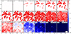 |
Fig. 1. Timeline of δTb. The colour bars are in units of [mK]; ⟨δTb⟩ represents the mean of the temperature brightness. These maps come from a 21cmFAST simulation, taken at a given depth from the model ζ55 and for each redshift used in this study. White corresponds to the absence of signal, meaning that the hydrogen is ionised at this region. For this simulation, at z = 5.5, there is no neutral hydrogen anymore. Starting at z = 15, δTb is mainly seen in absorption (negative values in blue) until z = 11, where ⟨δTb⟩ becomes positive and the signal is seen in emission (positive values in red). During the whole process, HII bubbles grow with time. Figure 2 corresponds to the treion(r) associated to these maps. |
To obtain this chronology we can use the reionisation time field treion(r) (Chardin et al. 2019). Mapped on 2D images (see Fig. 2), treion(r) returns the time of reionisation for each pixel of the map and encodes the complete history of ionisation propagation in a single field. In Thélie et al. (2022a), it was shown how its topology contains a wealth of information on the reionisation process. For example, treion(r) minima are the seeds of the propagation fronts where presumably the first sources can be found, treion(r) isocontours track HII bubbles at a given time or its skeleton provides the sites of ionisation front encounters. It also gives information on the influence of radiation sources on each other (Thélie et al. 2022b), opening the door to study distant radiative suppression by nearby objects in the environment. More generally, treion(r) gives information on local reionisations rather than the global reionisation, putting an emphasis on the environmental modulation of the ionisation history. This local modulation of how light is produced and propagates can translate into local variations of star formation suppression (see e.g. Ocvirk et al. 2020) or influence the spatial distribution of low-mass galaxies (see e.g. Ocvirk & Aubert 2011). Galaxies experience a great diversity of reionisation from their point of view (e.g. Aubert et al. 2018; Zhu et al. 2019; Sorce et al. 2022), and the reionisation time distribution probes this diversity. Other examples of using a similar description include Trac et al. (2008) on the thermal imprint of local reionisations, Trac et al. (2022) for reionisation modelling, or Deparis et al. (2019) for ionisation front speed measurments. It should be noted that these specific examples use reionisation redshifts instead of reionisation times; while directly related, we found that times are more easily reconstructed than redshifts for our purposes (see Appendix), and we focus only on reionisation times in this paper.
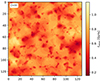 |
Fig. 2. Example of 2D treion(r) map from a ζ = 55 21cmFAST model. The darker the region, the sooner it reionised. In this scenario (and for the whole ζ55 dataset), the time of reionisation of the first HII regions is approximately 0.15 Gyr (z ≈ 20, darkest spots), and the last HI regions are reionised at around 1.1 Gyr (z ≈ 5.5, brightest regions). The mean value is 0.61 Gyr (z ≈ 8.4). This treion(r) map is associated with Fig. 1, taken at the same depth in the simulation box. |
As a means to predict treion(r), we use convolutional neural network (CNN) methods, which are capable of detecting and learning complex patterns in images. This tool has been widely used in different problems of astrophysics and cosmology (e.g. Bianco et al. 2021; Gillet et al. 2019; Chardin et al. 2019; Prelogović et al. 2022a; Ullmo et al. 2021). In a recent study Korber et al. (2023) successfully retrieve the growth history of bubbles using mock physical fields. In this study, we extend the CNN applications to treion(r) field reconstructions from mock observations of the 21 cm signal using a U-shaped convolutional neural network (Ronneberger et al. 2015), which allowed us to get the whole history of reionisation of a sky patch from a single observation.
This article is structured as follows. In Sect. 2 the CNN algorithm and the procedure to deal with the analysis are described. We also present the simulations used to obtain the data. In Sects. 3 and 4 we present the metrics used and the results obtained from monitoring the neural network performance. We discuss instrumental effects in Sect. 5, and give more information about choices made for this study in Sect. 6. Finally, we conclude in Sect. 7.
2. Convolutional neural network and simulation
The main purpose of this study is to reconstruct the spatial distribution of the reionisation times from 21 cm images using a convolutional neural network (CNN). CNNs are often used to process pixel data, and became widely used for image recognition (LeCun et al. 1999). Our neural network is implemented thanks to the Tensorflow (Abadi et al. 2015) and Keras (Chollet 2015) Python libraries. It took root in the well-known U-net network first developed by Ronneberger et al. (2015). The particularity of this network architecture lies in two distinct parts (Fig. 3). The first part is a contracting path called the encoder, applying series of 2D convolutions and downsamplings to the input image (a 21 cm map here) where its size shrinks as it goes deeper through the neural network. Then the second part does the opposite; it consists of an expansive path (the decoder) applying the same number of convolutions with upsamplings to propagate the information obtained in the encoder. The resulting final output is then another image, treion(r) in our case. This special case of CNN is called an auto-encoder.
 |
Fig. 3. Convolutional neural network used in this work. The Encoder (left) refers to the first sequence of 2D convolutions and Max Pooling operations, while the Decoder (right) refers to the second sequence of 2D convolutions and upsampling operations. Each Max Pooling operation reduces the input map size by a factor of 2, keeping mainly large-scale information. The upsampling operator does the opposite, propagating the information at larger scales and increasing the input map size. Each convolution modifies the number of filters in such a way that we have the maximum number of filters at the deepest point of the network. Dropout and skip connection layers are depicted with black asterisks and purple arrows, respectively. Each square contains the size of the feature maps, which remain consistent along a given horizontal line (see Appendix A for additional details about the CNN model). |
For the learning process, we generated a dataset of histories of reionisation, with their corresponding sequence of 21 cm maps. One CNN predictor was considered for each zobs redshift at which we have mock 21 cm observations. In practice, we considered 18 predictors for each zobs shown in Fig. 1. Ideally, all CNN predictors create the same treion(r) map from mock observations drawn from the same reionisation history. However, depending on the specific properties of a given 21 cm observation (e.g. the non-zero signal fraction) at a given zobs, the predictions will not perform equally well.
The public 21cmFAST simulation code (Mesinger et al. 2011; Murray et al. 2020) was chosen to obtain the dataset (i.e. 21 cm signal and treion(r) fields). Coeval simulations cubes of size 256 cMpc h−1 with resolution 1 cMpc h−1 pixel−1 were produced using a ΛCDM cosmology with (Ωm, Ωb, ΩΛ, h, σ8, ns) = (0.31,0.05,0.69,0.68,0.81,0.97) consistent with the results from Planck Collaboration VI (2020) and using standard (Tvir, ζ) parameters. The parameter Tvir sets the minimal virial temperature for halos to enable star formation (see Gillet 2016; Muñoz et al. 2020; Barkana & Loeb 2001) and Oh & Haiman 2002) and was chosen such that log10(Tvir) = 4.69798. The parameter ζ sets the ionising efficiency of high-z galaxies, and allows us to modify the reionisation timing: the larger this value is, the faster the reionisation process will be (Greig et al. 2015). We considered two ionising efficiencies ζ = 30 and ζ = 55 (referred as ζ30 and ζ55), leading to a total of 36 CNN models to be trained, 18 redshifts per ζ value. For each ζ, 50 different realisations with different seeds were run, giving us access to treion(r) and 21 cm 3D fields. As discussed in the introduction, an alternative approach is to consider the reionisation redshift zreion(r) instead of treion(r). However, we found that the times were better reconstructed, and a brief analysis using zreion(r) is presented in Appendix B.
To produce 2D images of treion(r) and the 21 cm signal, we took 64 evenly spaced slices, one out of four (of 1 cMpc h−1 thickness, corresponding to one cell), in the three directions of each cube. Each slice was cut into four 128 × 128 images, finally leading to a total of 768 21 cm images per realisation and per z, giving 38 400 maps per redshifts. We standardised the 21 cm images to ensure that the range of pixel values was consistent across all images in the dataset and to help the model’s training process. The mean value was subtracted and the result was divided by the standard deviation (std), both computed over the training set. The mean and standard deviation values are thus the parameters of our predictors.
As shown in Fig. 4, the neutral volume fraction QHI is shifted (on the time axis) according to the ionising efficiency ζ. Since ζ controls how many photons escape from galaxies, ζ30 gives a delayed history of reionisation compared to ζ55. We discuss below the non-zero signal fraction (i.e. the fraction of pixels with non-zero 21 cm signal). Its time evolution is plotted as dots and crosses in Fig. 4, and is shown to follow QHI.
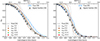 |
Fig. 4. Neutral fraction of hydrogen with respect to time (bottom axis) and redshift (top axis) for ζ30 (left panel) and ζ55 (right panel). The crosses stand for the average non-zero signal fraction obtained from 21 cm images at different values of z (as if taken along the line of sight). The dashed areas stand for the true QHI computed from true maps of treion(r) (mean and std). The dotted lines stand for the average QHI obtained from maps of treion(r) predicted by the CNN. |
The entire dataset is split into three subsets, from which 35 000 images are used for the learning phase. The first subset, known as the training set, comprises 31 500 images. At each epoch during the learning phase this set is fed to the CNN, which computes the loss function (i.e. mean square error, MSE in our case) and modifies the weights to minimise it. Another separate subset of the entire dataset, called the validation set, consists of 3500 images; it is exclusively used to evaluate the CNN’s performance during the learning phase after each epoch, without being used in the weight adjustment process. The final set is called the test set, and consists of the remaining 3400 images, which are never processed by the CNN during the learning stages. All the results shown in this paper (except for the loss function and R2; see Sect. 3.1) were obtained via the test set.
3. Monitoring the algorithm performance
Once all the hyper-parameters were set and predictions made, we measured the training performance and the prediction accuracy by comparing the predicted treion(r) maps with the ground truth given by the 21cmFAST simulation.
3.1. Network internal metrics
First, two internal metrics were used to monitor the training process. Starting with the loss function, the mean square error (MSE) was defined as the average of the squares of the errors. At each epoch the algorithm tries to minimise this loss function (MSE) by comparing the ground truth (given by the simulation) with the prediction (given by the CNN).
A second indicator was used, called the determination coefficient, defined as
 (2)
(2)
where Pred and True are the treion(r) maps of the prediction and ground truth, respectively; Predn and Truen correspond to the n-th pixel of the considered batch of images; and  depicts the average of the true field and is equal to zero after normalisation. In our case the predicted values, Pred, and the ground truth values, True, are both (3500, 128, 128) cubes. The summations are performed over Npix pixels to measure the network performance on a set it has already or never seen (training or validation set, respectively). Identical values of PRED and TRUE lead to R2 = 1.
Figure 5 shows the R2 coefficient during the validation phase for several observation redshifts zobs and for ζ55. For the validation set, this coefficient gives a first estimation of the similarities between true fields and predicted fields immediately at the end of each epoch, allowing us to follow the model’s accuracy during the learning process. At low redshift the R2 coefficient is small and, even worse, negative for this model and for the lowest z. Nothing can be predicted from low redshift ranges since the non-zero signal fraction at small zobs ∈ [5, 7] is low or even equal to zero. Then, above a value of 8 we observe that the prediction performance increases for increasing zobs until 11, where it eventually degrades again until 15.
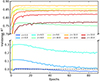 |
Fig. 5. R2 coefficient with respect to epochs for a selection of training redshifts. These curves correspond to the validation phase and are for the ζ55 model. The curves for ζ30 are not shown here, but a comparison between the two models is shown in Fig. 6. |
Figure 6 shows the maximum value across epochs for R2 for each zobs and the two ζ models, as well as the minimum value reached by the MSE loss. According to these metrics, the best reproduction of treion(r) is obtained from the CNN predictor using 21 cm maps at zobs = 11, corresponding to 95% of non-zero signal (see Fig. 4). Furthermore, the ζ30 model returns better results at lower zobs: at zobs = 7,  for ζ30, while
  for ζ55. This can be easily understood from Fig. 4, where the non-zero signal fraction of ζ30 is considerably larger than for ζ55 in the zobs range [5,8] (top axis): at zobs = 7, QHI > 40% for ζ30, while < 17% for ζ55. At this range of signal fraction values, the gain in terms of information is such that the network performance increases significantly. From Figs. 4 and 6, we can estimate that between [0.90,0.96] of non-zero signal fraction the neural network achieves better performance. For a non-zero signal fraction greater than 0.96, the performance decreases again. At these levels of non-zero signal fraction there are only a few HII bubbles to be found, inducing a loss of information on the location of the seeds of most reionisation regions. Without HII bubbles, the sources of reionisation cannot be located and the UV radiation propagation cannot be determined. Hence, in order to get the best performance, the CNN algorithm requires a compromise between a minimal set of HII bubbles and a significant non-zero signal fraction. The peak value of R2 = 0.88 at z = 11 also suggests that this redshift of observation is peculiar. The timeline in Fig. 1 shows that z = 11 seems to be the transition between a global negative temperature brightness and a positive one in our model as the long range influence of X-rays on the gas becomes effective. At this zobs the 21 cm map contains small HII regions with no signal, easily interpretable for the CNN as the places where the first seeds of reionisation are found. Then there are regions that are hotter than average (shown in red) that will reionise sooner, and blue regions that are colder than average that will be the last regions to reionise. This zobs thus contains information of the sequence of radiation propagation that seem to be more easily extracted compared to other observation redshifts.
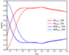 |
Fig. 6. Metric maximum and minimum with respect to the training redshift for the validation set. The red line is for the coefficient R2 and the blue line is for the MSE. The solid lines are for ζ55 and the dashed line for ζ30 model. |
3.2. Reionisation time prediction
Beyond the CNN internal metrics, the immediate result is the predicted map itself, as shown in Fig. 7. This zobs = 11 map is one of the best reconstructions (R2 = 0.84) we could create for the ζ30 model. The predicted map on the right seems quite close to the ground truth, but smoother. We note that the best predicted maps for ζ30 and the best predicted maps for ζ55 (not shown here) present a similar qualitative behaviour.
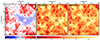 |
Fig. 7. Example of prediction done by the CNN trained from images at zobs = 11 and for ζ30 model. The left panel shows the 21 cm signal δTb at this redshift. The middle panel is the ground truth of the treion field. The right panel is the CNN prediction for treion obtained from δTb (left panel). |
With the true map of treion(r) and its prediction, we can count the number of pixels with values larger than a given reionisation time to obtain QHI(t) on the sky (see Fig. 4). For zobs = 11, both TRUE and PRED measurements match within the dispersion of true values and are consistent with the signal fraction evolution computed from the actual evolution of the 21 cm signal with z. This implies that the information obtained across the sky at a single zobs via the predicted treion(r) is consistent with (or can be cross-checked against) the evolution along the line of sight.
Figure 8 shows examples of predictions obtained for different models trained at different zobs. The first column shows the mock observations (21 cm maps) at several redshifts, the middle column shows the predictions obtained with the left panel and the right column shows the difference between the ground truth and the predicted treion(r) field. Looking at the two first columns, at low redshift, the predictions are suboptimal as the inferred field has been completely smoothed. For zobs ≥ 10, Our CNN becomes able to capture small-scale features (< 10 cMpc h−1), such as extrema. However, in the right column the CNN seems to have more difficulties in predicting the local extrema of reionisation times, even though their locations are well predicted, especially at low redshift (e.g. for zobs = 8: (x, y)≈(120, 125) cMpc h−1). These points correspond to the seeds of the propagation of fronts, presumably linked to the first sources of radiation, and seem to be subject to a smoothing intrinsic to our CNN implementation. Compared to zobs = 10 or 11, the zobs = 15 prediction appears to be slighty smoother, although the earliest reionisation times seem to be well reproduced. Finally, Fig. 9 depicts the normalised histogram of TRUE-PRED maps. Distributions are centred on zero, with an assymetry towards negative values: our CNN predictions returns greater reionisation times than the ground truth (i.e. a delayed reionisation history). For example, taking zobs = 15 there are more pixels at True-Pred = −0.4 Gyr (dN/dt > 2e − 4) than for True-Pred = 0.4 Gyr (dN/dt < 3e − 5). This systematic effect is less severe for the best CNN predictors trained to process zobs = 8 or 10.5 observations in this figure.
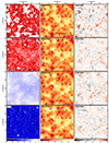 |
Fig. 8. Examples of prediction made by the CNN trained with maps at several redshifts zobs and ζ30. The left panels show the 21 cm δTb maps. The middle column shows the predicted treion fields. The right panels show the difference TRUE-PRED. Hence, the redder it appears on the map, the more the CNN overestimates the true value at the given pixel; instead, the darker it is, the more the CNN underestimates the real value. The true treion(r) is shown in Fig. 7. |
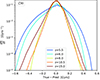 |
Fig. 9. Normalised distribution of TRUE-PRED values (as shown in Fig. 8) for several zobs. These curves were obtained from the whole test set of ζ30 models. |
3.3. True versus predicted histograms and fitting fraction
One of the most standard tests is the true versus predicted (TvP), where all the predicted pixels are compared one by one to their true value given by the simulation. Figure 10 shows the TvP corresponding to all the maps in the test set using the zobs = 11 CNN. Most values follow the perfect correlation for typical treion(r) values (0.4–1 Gyr), while extreme values (< 0.4 Gyr and > 1 Gyr) are not as well recovered by the CNN (mean value up to +0.25 and down to −0.15 respectively). This is not surprising, given the predicted maps on Fig. 7. The extreme values of treion(r) coincide with small-scale features that are smoothed out, where the first sources with lowest treion are found. These values are also rare (4.2% of the total number of pixels), explaining why the algorithm fails at learning how to recover them.
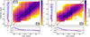 |
Fig. 10. True vs predicted maps obtained from the full dataset in the test set, for zobs = 11 and for both models. The red lines stand for the perfect correlation. The bottom and left histograms are the mean and the standard deviation of the residual r: r = Predicted−True, in both vertical and horizontal directions. The bottom histogram stands for the learning error, while the side histogram stands for the recovery uncertainty. In practice, the recovery uncertainty is the only accessible estimator since the ground truth will not be accessible. |
Figure 11 presents a synthesis of the true versus predicted maps of all the predictors at different zobs. The fitting fraction is a value between 0 and 1, which corresponds to the predicted pixel’s fraction whose value fits within an arbitrary error calculated as ϵ% of the true pixel’s value. The larger the allowed error is, the more ‘good’ pixels will be found. It is then clear how low zobs values (< 8) gives less accurate results, especially when allowing a small error (< 10%): the fitting fraction value is more than 10% lower than for zobs > 8. It can be understood from the maps of temperature brightness (or from Fig. 4) where the maps contain less signal with decreasing redshifts from z = 8: less than 50% of the map contains observable neutral hydrogen. At the extreme redshift z = 5.5 there is no signal left because all HI is reionised and no prediction is possible. A value of zobs > 8 seems to give the best results, and all predictions made from zobs above 9 seem to have similar performance: between 70 and 75% of matching pixels for 5% error, and a slight decrease with growing zobs. Overall, we recover the two trends identified previously: low zobs simply lacks the signal for a good reconstruction, while high zobs lacks the direct imprint of sources that appear later. The best compromise is found for zobs values between 8 and 12, corresponding to signal fraction ≈0.8, with an optimal value of 0.95.
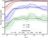 |
Fig. 11. Fitting fraction with respect to redshift. The greater the allowed error for a pixel (between prediction and ground truth) is, the larger the number of pixels that have a value close to the true one within this error (i.e. ‘good pixels’). The solid lines are for ζ55 and the dotted lines for ζ30. The shaded areas depict the standard deviation around the mean for the whole predicted dataset. |
3.4. ζ30 and ζ55
The first results comparing the ζ30 and ζ55 scenarios are very close. The prediction accuracy is similar except for lower zobs (< 8) where the signal fraction tends to be quite different between both situations. In the most extreme case, at zobs = 5.5, the CNN trained with the ζ30 maps is quite limited, but still returns a prediction, whereas the CNN trained with ζ55 maps cannot predict anything, which was expected since there is no HI left at late times in the ζ55 scenario. In the following sections, we only consider the ζ30 scenario to discuss results in the whole range of zobs used.
4. Structure of predicted maps
We now investigate the spatial structure of the reconstructions using three metrics: the power spectrum, the Dice coefficient, and the minima statistics.
4.1. Power spectrum Pk
We now compare the power spectrum Pk of the reionisation time field with that predicted by the neural network in order to have a statistical point of view on how well the network reconstructs the different scales present on the map. Figure 12 depicts the treion(r) power spectrum of model ζ30. A first look shows that the lack of 21 cm signal drastically erases the possibility to predict anything. Predictions for z = 5.5 and z = 6 are incompatible with the real Pk at mid-scales k ≈ 7e − 2 cMpc−1 h; less than 30% of the power remains for z = 6, against up to 85% for z = 8. At small scales (k > 2e − 1 cMpc−1 h) less than 12% of the power remains for z = 6 against up to 57% for z = 8. Now looking at large scales (low spatial frequencies such as k < 3e − 2 cMpc−1 h), our model reproduces the power at more than 95% for zobs > 8. However, at k = 0.2 cMpc−1 h and beyond, the prediction cannot produce enough power, meaning that the smaller scales are difficult to predict at all zobs. Again, the predictor smoothes the treion(r) field, predicting a map generally blurrier than the ground truth. To improve results at the smallest scales, generative adversarial networks (GANs) could be a solution (see Ullmo et al. 2021).
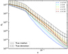 |
Fig. 12. Power spectrum of the treion(r) field obtained for ζ30. k is the spatial frequency with dimension [cMpc−1 h]. The black line stands for the average power spectrum of the ground truth and the dotted coloured lines stand for P(k) predictions with different zobs. The shaded areas depict the dispersion around the median (1st and 99th percentiles) for both predictions and ground truth. |
4.2. Dice coefficient
Another way to look at the predictor performance is the Dice coefficient (see Ullmo et al. 2021). This method is useful to see what kind of regions the algorithm reconstructs best; for example, whether the first regions that become reionised are clearly predicted or if, conversely, late regions are reconstructed in a better way. This coefficient focuses on the map structure by looking at regions with given values. It determines how the CNN recovers structures instead of giving an accuracy according to the value of pixels or the considered scale.
The Dice coefficient is used by taking a threshold t (0 to 100) and by considering only the pixels with the largest treion values in the true and predicted maps. We can estimate the regions of the map where the prediction overlaps with the ground truth, using a newly formed map with pixels in only three possible states:
-
Predicted and true pixels both have a value above the threshold (both fit the criterion), denoted the yellow state.
-
Both have a value below the threshold (both do not fit the criterion), denoted the blue state.
-
There is a mismatch between the prediction and simulation, denoted the green state.
It is important to note that the value of the threshold corresponds to a given cosmological time (or redshift). Using 10% for the threshold, the constructed map will only contain the information for large values of cosmological time (low redshifts), typically the last regions to reionise. On the other hand, taking 100% as threshold, the whole map will be considered. An example of an overlap map is depicted in Fig. 13 using zobs = 10. The threshold example on the figure is 0.4, corresponding to 40% of the largest values. Only a few green regions (corresponding to 15% of the pixels) are present, and more than 85% of the pixels are in agreement between the prediction and the ground truth. This range of values is actually well reconstructed, and the remaining differences are located at the edge of these regions (in the green areas, e.g. (x, y)≈(70, 10) cMpc h−1).
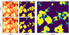 |
Fig. 13. Example of overlap map for ζ30 and a threshold value t = 0.2. The left panel is the true treion field (top) and the predicted treion(r) for a zobs of 10 (bottom). The middle panel depicts a 1 or 0 map where 1 (yellow) stands for the pixels fitting 20 % of the highest values and 0 (purple) for pixels below the threshold for the true field (top) and the predicted field (bottom). The right picture is the overlap of the middle panels, where yellow stands for coincidence, green for incorrect pixels in the prediction, and purple where the values are below the threshold in both fields. |
The Dice coefficient, or association index, is calculated at a given threshold as (Dice 1945)
 (3)
(3)
with ni the number of pixels with colour i. The Dice coefficient can only take values between 0 and 1 (0 for no correspondence between prediction and ground truth and 1 for a perfect reconstruction).
Figure 14 shows the Dice coefficient for the ζ30 model. The dotted black line stands for the Dice coefficient obtained if we compare the true thresholded map with a map randomly filled with zeros and ones. Globally, we recover that zobs > 8 provides better accuracy compared to the random situation (for threshold = 0.4: Dice > 0.7 against 0.4, respectively), with similar performance at all zobs. Furthermore, zobs = 11 seems to dominate until median values for the threshold. Afterwards, zobs = 8 coefficents catch up, followed by zobs = 10, meaning that these observation redshifts recover efficiently the first structures of reionisation.
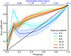 |
Fig. 14. Dice coefficient for several zobs and for ζ30. The dashed black line stands for the Dice coefficient when matching the true map with a random mask. Pixels are considered starting with the largest pixel value (last pixel to reionise) down to a threshold. A 0.2 threshold means that we consider the last 20% to be reionised. The shaded areas depict the standard deviation around the mean DICE coefficient. |
Looking at low threshold values, the Dice coefficient provides additional insights into the performance at low zobs, such as zobs = 5.5 or 6. At these redshifts, predictions are slightly better for low threshold values meaning that at zobs = 6, the neural network predicts in a very efficient way the last regions reionised (for threshold = 0.1, Dice > 0.9): since they are the only regions where a non-zero signal can be found, the predictor can locate them accurately.
4.3. Minima statistics
We now investigate at the minima of treion(r) (i.e. the regions that reionised at the earliest times) to probe how our CNN detects sources of reionisation. We used the Discrete Persistent Structures Extractor (DisPerSE) (Sousbie 2011; Sousbie et al. 2011) to identify the distribution of reionisation times minima; it uses discrete Morse theory to identify persistent topological features in two-dimensional maps, such as voids, walls, filaments, and clusters. While we focus here only on minima, valuable insights into the underlying topology of treion(r) can also be obtained from the persistent structures detected by DisPerSE, to see how they relate to the physical processes that shape the distribution of reionisation (see also Thélie et al. 2022a,b).
The results of this analysis are illustrated in Fig. 15. The black line stands for this analysis performed on the true treion(r) field: at low treion (high z) sources are rare, and their number is highest at t = 0.8 Gyr (approx z = 7). Their number then drops at higher treion(r) values, not because sources becomes rarer but because they appear in already reionised regions and cannot be traced by peaks in treion(r) maps. The statistics of our CNN predictions, depicted with dotted lines, clearly show that the CNN has some difficulties to detect the first sources of ionising photons (treion(r) < 0.4), resulting from the smoothing of treion(r) maps. However, the maximum of the distribution is well matched at least for zobs > 8, whereas low zobs = 5.5 − 7 predictors fail unsurprisingly to recover the seeds of ionisation fronts from 21 cm maps with very low non-zero signal fractions. Interestingly, an observation made for example at zobs = 10 manages to predict in a satisfying manner, by being consistent with dispersion of time distribution, the population of peaks (and thus seeds and/or sources of reionisation) at later times (treion = 1 Gyr), emphasising the ability of our CNN to extrapolate the future of a given observation. When compared with the previous power spectrum analysis, these results emphasise that the loss of accuracy on small scales mostly have an impact on high-z (low treion) peaks, whereas the seeds of ionisation fronts at lower redshifts are much better predicted with the lowest zobs.
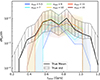 |
Fig. 15. Distribution of reionisation times for treion(r) minima. The solid line is obtained from true treion(r), while the dotted lines are obtained from predictions at several zobs. The shaded areas show the dispersion around the median (mean and std) for both predictions and ground truth. |
5. Instrumental effects and prediction
The work discussed previously only takes into account a ‘perfect’ 21 cm signal, without any noise or instrumental effect. Studying the effect of foreground contamination and how to manage it is of primordial importance to being able to properly analyse the future observation. While this paper does not delve into these effects, this section aims to shed some light on them. Nonetheless, there are other studies in the field of deep learning that specifically address the impact of foreground contamination, such as the work by Bianco et al. (2023). These effects are expected to degrade the predictor’s capability to infer the treion(r) field. As a means to study the potential impact of these effects in our predictions, we created a new dataset of 21 cm maps with instrumental and noise characteristics corresponding to SKA. The UV coverage and instrumental effects are calculated using the tools21 cm4 library (Giri et al. 2020), assuming a daily scan of 6 h, 10 s integration time, for a total observation of 1000 h (Prelogović et al. 2022b; Ghara et al. 2016; Giri et al. 2018). Our investigation is limited to zobs = 8, corresponding to the lowest redshift where the predict or accuracy in terms of the R2 coefficient remains satisfying (R2 = 0.86), while deeper observations are found to be significantly more degraded by noise. A maximum baseline of 2 km is assumed and the angular resolution is Δθ ∼ 2.8 arcmin, corresponding to 7.35 cMpc at this redshift. The tools21cm library also convolves the coeval 21 cm cube in the frequency direction with a matching resolution Δν ∼ 0.43 MHz. Figure 16 shows the prediction from noisy observations with the input 21 cm observations shown in the left panel. The predicted treion(r) map is much blurrier at first sight; adding instrumental effects on input observations smoothes the prediction even more.
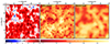 |
Fig. 16. Predictions for the model ζ30 at zobs = 8, including instrumental effects for a typical SKA observation (left panel, see details in main text). The middle panel is the ground truth for treion(r) and the right panel is the CNN prediction. |
Figures 17 and 18 depict the power spectrum of the treion(r) field and QHI for ζ30, for both ground truth and prediction. The two predicted curves (dotted lines) have been implemented with observation at z = 8, one with instrumental noise (in blue) and the other using a perfect 21 cm map (in red). In both predictions the power spectrum is successfully recovered at large scales (k < 3e − 2 cMpc−1 h), with approximately 70% and 95% of the remaining power for the noisy case and perfect case, respectively. At smaller scales (k > 2e − 1 cMpc−1 h) the power spectrum recovered from noisy maps has a sharper turn-off (17% of power remaining against 86% for the perfect case) and comes out of the error bars (hatched and shaded areas). It results in missing the small-scale structures, making it difficult and even impossible, to detect the first sources of reionisation accurately. On the other hand, QHI gives a fair history of reionisation, although more sudden from SKA maps than the ground truth and the perfect signal scenario: noisy reionisation ends around treion = 1 Gyr and the perfect scenario ends around 1.1 Gyr.
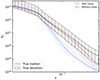 |
Fig. 17. Power spectrum of the treion(r) field obtained with the model ζ30 at zobs = 8, including instrumental effects for a typical SKA observation. The black line and hatched area stand for the mean and standard deviation of the true field P(k). The dotted lines and shaded area depict the median and dispersion (1st and 99th percentiles) of CNN predictions P(k) with (blue) and without (red) instrumental effects. |
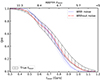 |
Fig. 18. QHI obtained from predictions at zobs = 8 with the model ζ30, including instrumental effects for a typical SKA observation. Hatched area stands for the true field QHI. Dotted lines and shaded area depict the mean and standard deviation of CNN predictions QHI with (blue) and without (red) instrumental effects. |
This outcome raises several questions. The first is linked to the architecture of the CNN, and whether it is possible to improve the CNN such that the accuracy of the prediction improves significantly, especially for noisy observations. For this purpose a solution could be to tune the hyper-parameters in order to find the best combination to recover treion(r). In addition, keeping the U-shaped CNN and modifying the number of hidden layers or filters, or the deepness of the algorithm could change the prediction in the right direction. Another possibility could be to add an attention block to help our CNN to focus on small-scale features (Oktay et al. 2018). Using GANs (Ullmo et al. 2021) could also improve the output field in order to recover small scales (k > 2e − 1 cMpc−1 h). Another solution would be to preprocess the noisy 21 cm observation in order to remove or reduce noise and instrumental effects. In such a situation we would hopefully recover a perfect observation scenario, drastically boosting the prediction accuracy.
6. Discussion and perspectives
The work presented in this paper has involved numerous decision-making processes that may have been influenced by factors such as default settings, initial ideas, and implementation challenges. When it comes to the architecture and hyper-parameters of the CNN algorithm, the choices made are typically based on the fact that they yield improved performance (in terms of R2). However, some choices, such as the number of filters, the inclusion or location of dropout layers, or the choice of loss function for weight adjustment, can potentially be modified; it is conceivable that untested combinations of hyper-parameters might yield better results. Ongoing investigations are being conducted to further explore this matter.
Another decision was to use images of the 21 cm signal at a single redshift or frequency, leading to one CNN per redshift (and per model). A possibility would have been to train the predictors with multiple redshifts channels or even light cones. This could possibly help the predictors to infer maps even in the regime of low non-zero signal fraction at low zobs (< 8); the inclusion of higher zobs information in the prediction process can provide additional constraints (e.g. on the global reionisation history) that cannot be inferred from single low zobs 21 cm maps alone. Our choice is largely the result of the history of this work, where it was not obvious at first that any prediction would have been possible, even in the case of a perfect 21 cm signal. Investigations are currently ongoing to see what can be gained from a multiple channel prediction.
However, we also believe that having multiple CNNs has some merit regarding the adequacy of the parameters (cosmological, astrophysical) of a predictor to the parameters that drive a given 21 cm observation. In a real case scenario, the ‘real’ parameters of an observation are unknown, and we therefore face a situation where it is unclear which CNN should be used to reconstruct treion(r). One possibility is to assume that the model parameters will be obtained from another analysis (e.g. using the 21 cm power spectrum) and the role of a CNN predictor is therefore limited to reconstructing the spatial distribution for the reionisation times in a specific observation. However, preliminary investigations also show that when a set of 21 cm maps at different zobs are processed by the multiple predictors of a ‘wrong’ model (for example ζ55 maps in ζ30 predictors), they lead to a set of treion(r) maps that are inconsistent, for example with regard to their average reionisation history. Meanwhile, a CNN that can reconstruct multiple treion(r) at once from multiple 21 cm maps would always, by construction, ensure some consistency between its predictions, even for a wrong model. The optimal situation is likely to be an intermediate situation with CNNs dedicated to reconstruct a given zobs, but that use multiple 21cm maps at different redshifts.
7. Conclusions
In this study, we implemented and tested a U-net architecture to infer the treion(r) field from 21 cm maps simulated by the 21cmFAST simulation code. These predictions are especially effective to recover the large-scale features (> 10 cMpc h−1) of reionisation times and can to some extent recover the past and extrapolate the future evolution of an observation made at a given zobs.
For our models, zobs values between 8 and 12 seem to provide the best results according to several metrics (e.g. R2, the Dice coefficient, power spectrum, true vs predicted), corresponding to a signal fraction of 65% up to 96% for the ζ30 model. For zobs < 8, even though the last regions to be reionised can be reconstructed, the lack of 21 cm signal in general significantly degrades the network’s capability to predict treion(r). For deep observations (zobs > 12), the CNN still manages to reproduce quite well the very first sources of reionisation due to the rare and narrow HII bubbles imprinted in the 21 cm signal, but has more difficulties to predict the location of sources that appear later, which leads to smoother maps. It also might be interesting to keep the information with low signal fractions (zobs < 8) since it reconstructs quite well the last regions to become reionised.
In addition, our CNN model works well at recovering the largest scales, as seen for example in the power spectrum analysis. Nevertheless, there are still some limits to what our network can do; for example, it has difficulties to recover the smallest scales (< 10 cMpc h−1). That could indeed be a problem to constrain physics related to small-scale structures (such as the physics of low-mass objects or that related to the nature of dark matter). It might be still possible to improve results at small scales with the use of GANs to generate a more detailed treion(r) field. In addition, implementing an attention block to insert it in our CNN could help predictors to focus on small-scale features.
Two scenarios have been used with different histories of reionisation. No significant difference in the training phase or in the prediction phase has been detected. The main difference comes at the lowest redshifts: the ζ55 scenario reionises sooner, lacks signal more rapidly, and is more difficult to predict for low zobs (< 8).
We believe that the method presented here can prove to be useful for the future interpretation of 21 cm data. First, it demonstrates that the information of reionisation times is encoded in the 21 cm signal. The field treion(r) gives access to chronology of light propagation in the transverse plane of the sky, that could be for example cross-checked with other estimates of the reionisation evolution obtained along the line of sight (21 cm light cones or Lyα/21 cm forests for example), and presumably it can be related to the global history of structure build-up and star formation. Another application would be the cross-correlation of reionisation time maps with galaxy distributions or intensity maps other than 21 cm; having access to the propagation history around objects observed through other channels could provide insights into their own local history of the production of light (and therefore of stars and sources) (see also e.g. Aubert et al. 2018; Sorce et al. 2022). There should also be an environmental modulation of star formation suppression by reionisation (e.g. Ocvirk et al. 2020; Ocvirk & Aubert 2011) and a map of reionisation times could provide a way to test this by providing an insight into how local reionisation proceeded. As illustrated in Sect. 5, the reconstruction of reionisation times from actual 21 cm data will be certainly be challenging, but surely holds some potential that we have not fully investigated yet.
Acknowledgments
The authors would like to acknowledge the High Performance Computing Centre of the University of Strasbourg for supporting this work by providing scientific support and access to computing resources. Part of the computing resources were funded by the Equipex Equip@Meso project (Programme Investissements d’Avenir) and the CPER Alsacalcul/Big Data. This work was granted access to the HPC resources of TGCC under the allocations 2023-A0130411049 “Simulation des signaux et processus de l’aube cosmique et Réionisation de l’Univers” made by GENCI. We also thank J. Freundlich for his help and advice. The authors acknowledge funding from the European Research Council (ERC) under the European Unions Horizon 2020 research and innovation programme (grant agreement No. 834148).
References
- Abadi, M., Agarwal, A., Barham, P., et al. 2015, TensorFlow: Large-Scale Machine Learning on Heterogeneous Systems, software available from tensorflow.org [Google Scholar]
- Abdurashidova, Z., Aguirre, J. E., Alexander, P., et al. 2022, ApJ, 925, 221 [NASA ADS] [CrossRef] [Google Scholar]
- Aubert, D., Deparis, N., Ocvirk, P., et al. 2018, ApJ, 856, L22 [Google Scholar]
- Barkana, R., & Loeb, A. 2001, Phys. Rep., 349, 125 [NASA ADS] [CrossRef] [Google Scholar]
- Bianco, M., Giri, S. K., Iliev, I. T., & Mellema, G. 2021, MNRAS, 505, 3982 [NASA ADS] [CrossRef] [Google Scholar]
- Bianco, M., Giri, S. K., Prelogović, D., et al. 2023, Deep Learning Approach Foridentification of HII Regions During Reionization in 21-cm Observations– II. Foreground Contamination [Google Scholar]
- Billings, T. S., La Plante, P., & Aguirre, J. E. 2021, Publications of the Astronomical Society of the Pacific, 133, 044001 [NASA ADS] [CrossRef] [Google Scholar]
- Chardin, J., Uhlrich, G., Aubert, D., et al. 2019, MNRAS, 490, 1055 [Google Scholar]
- Chollet, F. 2015, keras, https://github.com/fchollet/keras [Google Scholar]
- Dayal, P., & Ferrara, A. 2018, Phys. Rep., 780, 1 [Google Scholar]
- DeBoer, D. R., Parsons, A. R., Aguirre, J. E., et al. 2017, PASP, 129, 045001 [NASA ADS] [CrossRef] [Google Scholar]
- Deparis, N., Aubert, D., Ocvirk, P., Chardin, J., & Lewis, J. 2019, A&A, 622, A142 [NASA ADS] [CrossRef] [EDP Sciences] [Google Scholar]
- Dice, L. R. 1945, Ecology, 26, 297 [CrossRef] [Google Scholar]
- Furlanetto, S. R., Zaldarriaga, M., & Hernquist, L. 2004a, ApJ, 613, 1 [NASA ADS] [CrossRef] [Google Scholar]
- Furlanetto, S. R., Zaldarriaga, M., & Hernquist, L. 2004b, ApJ, 613, 16 [NASA ADS] [CrossRef] [Google Scholar]
- Furlanetto, S. R., Oh, S. P., & Briggs, F. H. 2006, Phys. Rep., 433, 181 [Google Scholar]
- Gazagnes, S., Koopmans, L. V. E., & Wilkinson, M. H. F. 2021, MNRAS, 502, 1816 [NASA ADS] [CrossRef] [Google Scholar]
- Ghara, R., Choudhury, T. R., Datta, K. K., & Choudhuri, S. 2016, MNRAS, 464, 2234 [Google Scholar]
- Ghara, R., Giri, S. K., Mellema, G., et al. 2020, MNRAS, 493, 4728 [NASA ADS] [CrossRef] [Google Scholar]
- Gillet, N. 2016, Ph.D. Thesis, University of Strasbourg, France [Google Scholar]
- Gillet, N., Mesinger, A., Greig, B., Liu, A., & Ucci, G. 2019, MNRAS, 484, 282 [NASA ADS] [Google Scholar]
- Giri, S. K. 2019, PhD thesis, Stockholm University, Sweden [Google Scholar]
- Giri, S. K., Mellema, G., & Ghara, R. 2018, MNRAS, 479, 5596 [NASA ADS] [CrossRef] [Google Scholar]
- Giri, S. K., Mellema, G., & Jensen, H. 2020, J. Open Source Softw., 5, 2363 [NASA ADS] [CrossRef] [Google Scholar]
- Gorce, A., Ganjam, S., Liu, A., et al. 2023, MNRAS, 520, 375 [NASA ADS] [CrossRef] [Google Scholar]
- Greig, B., & Mesinger, A. 2017, MNRAS, 472, 2651 [NASA ADS] [CrossRef] [Google Scholar]
- Greig, B., Mesinger, A., & Koopmans, L. V. E. 2015, arXiv eprints [arXiv:1509.03312] [Google Scholar]
- Hutter, A., Watkinson, C. A., Seiler, J., et al. 2019, MNRAS, 492, 653 [Google Scholar]
- Iliev, I. T., Mellema, G., Shapiro, P. R., et al. 2012, MNRAS, 423, 2222 [NASA ADS] [CrossRef] [Google Scholar]
- Karagiannis, D., Maartens, R., & Randrianjanahary, L. F. 2022, J. Cosmol. Astropart. Phys., 2022, 003 [CrossRef] [Google Scholar]
- Konno, A., Ouchi, M., Ono, Y., et al. 2014, ApJ, 797, 16 [Google Scholar]
- Korber, D., Bianco, M., Tolley, E., & Kneib, J.-P. 2023, MNRAS, 521, 902 [NASA ADS] [CrossRef] [Google Scholar]
- Kulkarni, G., Keating, L. C., Haehnelt, M. G., et al. 2019, MNRAS, 485, L24 [Google Scholar]
- Labach, A., & Valaee, S. 2019, Regularizing Neural Networks by Stochastically Training Layer Ensembles [arXiv:1911.09669] [Google Scholar]
- LeCun, Y., Haffner, P., Bottou, L., & Bengio, Y. 1999, Object Recognition with Gradient-Based Learning (Berlin Heidelberg: Springer), 319 [Google Scholar]
- Liszt, H. 2001, A&A, 371, 698 [NASA ADS] [CrossRef] [EDP Sciences] [Google Scholar]
- Liu, A., & Parsons, A. R. 2016, MNRAS, 457, 1864 [NASA ADS] [CrossRef] [Google Scholar]
- Loeb, A., & Barkana, R. 2001, ARA&A, 39, 19 [NASA ADS] [CrossRef] [Google Scholar]
- Mao, X.-J., Shen, C., & Yang, Y.-B. 2016, Image Restoration Using Convolutional Auto-encoders with Symmetric Skip Connections [arXiv:1606.08921] [Google Scholar]
- Mellema, G., Iliev, I. T., Pen, U.-L., & Shapiro, P. R. 2006, MNRAS, 372, 679 [NASA ADS] [CrossRef] [Google Scholar]
- Mellema, G., Koopmans, L. V. E., Abdalla, F. A., et al. 2013, Exp. Astron., 36, 235 [NASA ADS] [CrossRef] [Google Scholar]
- Mellema, G., Koopmans, L., Shukla, H., et al. 2015, Advancing Astrophysics with the Square Kilometre Array (AASKA14), 10 [Google Scholar]
- Mesinger, A., Furlanetto, S., & Cen, R. 2011, MNRAS, 411, 955 [Google Scholar]
- Mesinger, A., Ferrara, A., & Spiegel, D. S. 2013, MNRAS, 431, 621 [NASA ADS] [CrossRef] [Google Scholar]
- Mondal, R., Fialkov, A., Fling, C., et al. 2020, MNRAS, 498, 4178 [NASA ADS] [CrossRef] [Google Scholar]
- Mosbech, M. R., Boehm, C., & Wong, Y. Y. Y. 2022, Probing Dark Matter Interactions with SKA [Google Scholar]
- Muñoz, J. B., Dvorkin, C., & Cyr-Racine, F.-Y. 2020, Phys. Rev. D, 101, 063526 [CrossRef] [Google Scholar]
- Murray, S. G., Greig, B., Mesinger, A., et al. 2020, J. Open Source Softw., 5, 2582 [NASA ADS] [CrossRef] [Google Scholar]
- Nasirudin, A., Murray, S. G., Trott, C. M., et al. 2020, ApJ, 893, 118 [NASA ADS] [CrossRef] [Google Scholar]
- Ocvirk, P., & Aubert, D. 2011, MNRAS, 417, L93 [NASA ADS] [CrossRef] [Google Scholar]
- Ocvirk, P., Aubert, D., Sorce, J. G., et al. 2020, MNRAS, 496, 4087 [NASA ADS] [CrossRef] [Google Scholar]
- Oh, S. P., & Haiman, Z. 2002, ApJ, 569, 558 [NASA ADS] [CrossRef] [Google Scholar]
- Oktay, O., Schlemper, J., Folgoc, L. L., et al. 2018, Attention U-Net: LearningWhere to Look for the Pancreas [arXiv:1804.03999] [Google Scholar]
- Pagano, M., & Liu, A. 2020, MNRAS, 498, 373 [NASA ADS] [CrossRef] [Google Scholar]
- Planck Collaboration VI. 2020, A&A, 641, A6 [NASA ADS] [CrossRef] [EDP Sciences] [Google Scholar]
- Prelogović, D., Mesinger, A., Murray, S., Fiameni, G., & Gillet, N. 2022a, MNRAS, 509, 3852 [Google Scholar]
- Prelogović, D., Mesinger, A., Murray, S., Fiameni, G., & Gillet, N. 2022b, MNRAS, 509, 3852 [Google Scholar]
- Ronneberger, O., Fischer, P., & Brox, T. 2015, arXiv eprints [arXiv:1505.04597] [Google Scholar]
- Shaw, A. K., Chakraborty, A., Kamran, M., et al. 2022, Probing Early Universe Through Redshifted 21-cm signal: Modelling and Observational Challenges [Google Scholar]
- Sorce, J. G., Ocvirk, P., Aubert, D., et al. 2022, MNRAS, 515, 2970 [NASA ADS] [CrossRef] [Google Scholar]
- Sousbie, T. 2011, MNRAS, 414, 350 [NASA ADS] [CrossRef] [Google Scholar]
- Sousbie, T., Pichon, C., & Kawahara, H. 2011, MNRAS, 414, 384 [NASA ADS] [CrossRef] [Google Scholar]
- Thélie, E., Aubert, D., Gillet, N., & Ocvirk, P. 2022a, A&A, 658, A139 [NASA ADS] [CrossRef] [EDP Sciences] [Google Scholar]
- Thélie, E., Aubert, D., Gillet, N., & Ocvirk, P. 2022b, Topology of Reionisation Times: concepts Measurements and Comparisons to Gaussian Random Field Predictions [Google Scholar]
- Trac, H., Cen, R., & Loeb, A. 2008, ApJ, 689, L81 [NASA ADS] [CrossRef] [Google Scholar]
- Trac, H., Chen, N., Holst, I., Alvarez, M. A., & Cen, R. 2022, ApJ, 927, 186 [NASA ADS] [CrossRef] [Google Scholar]
- Ullmo, M., Decelle, A., & Aghanim, N. 2021, A&A, 651, A46 [NASA ADS] [CrossRef] [EDP Sciences] [Google Scholar]
- van Haarlem, M. P., Wise, M. W., Gunst, A. W., et al. 2013, A&A, 556, A2 [NASA ADS] [CrossRef] [EDP Sciences] [Google Scholar]
- Wise, J. H. 2019, ArXiv eprints [arXiv:1907.06653] [Google Scholar]
- Zaldarriaga, M., Furlanetto, S. R., & Hernquist, L. 2004, ApJ, 608, 622 [NASA ADS] [CrossRef] [Google Scholar]
- Zhao, X., Mao, Y., & Wandelt, B. D. 2022, ApJ, 933, 236 [NASA ADS] [CrossRef] [Google Scholar]
- Zhu, H., Avestruz, C., & Gnedin, N. Y. 2019, ApJ, 882, 152 [NASA ADS] [CrossRef] [Google Scholar]
Appendix A: CNN architecture details and hyper-parameters
In this section we describe the details of the CNN algorithm used in this study. We used the Python libraries Tensorflow (Abadi et al. 2015) and Keras (Chollet 2015) to implement our CNN. Table A.1 shows properties of the hidden layers. A convolution layer consists in applying a filter of a given size (3x3 in this study) to the whole input resulting in a featured map. Each convolution is performed with same padding, meaning that each convolution conserves the size of the input. For the encoder part, the first four convolutions are followed by a Max Pooling operation (of size 2x2) that is shrinking the size of the input by a factor of 2. When the 2x2 matrix passes through the input, it only conserves the pixel with the highest value. Dropout (Drop) layers are also used in order to help the CNN to prevent overfitting (Labach & Valaee 2019). A dropout layer acts by shutting down a given fraction (0.5 for us) of neurons/filters in the corresponding hidden layer where it is applied. For the decoder part, each convolution is followed by an UpSampling layer that doubles the size of the input. In addition, a concatenated layer (Merge or skip connection) is applied to fuse features of a given hidden layer within the encoder with features of the same size in the decoder. In practice, skip connections tend to improve the accuracy of CNN and to make it converge faster (Mao et al. 2016). Eventually, the activation function for each layer is Relu, except for the last one that is a linear activation function since we want to predict an output field with continuous values. During the learning phase of a CNN algorithm, the weights of each convolution filter are updated each time a batch of data is passed through. In our implementation, we set the hyper-parameter batch size to 16. This means that our model updates its weights after processing each batch of 16 images, and that one epoch is completed after N batches have been processed, where N is the number of batches needed to cover the entire dataset. In addition, to optimise the performance of the CNN algorithm, we needed to carefully choose the hyper-parameters. Some of them have already been discussed, such as batch size, dropout, and loss function. The ‘optimizer’ hyper-parameter was set to Adam. Another important factor is the initial weight of the model. The ‘kernel_initializer’ hyper-parameter controls this and was set to ‘He Normal’. However, because the weights are randomly initialised, there is a possibility that the learning process may get stuck in a local minimum without learning any more. To prevent this, we added a feature to the code that restarts the weight initialisation if such a situation is detected.
Details of the architecture the CNN used to predict maps of treion(r).
Appendix B: Using zreion(r) instead of treion(r)
The redshift of reionisation zreion(r) and treion(r) are two fields depicting the same quantity: the time of reionisation of regions in the sky, with zreion(r)∼treion(r)−2/3 during the reionisation epoch. We can investigate how choosing redshift instead of time affects the capability of the CNN to predict zreion(r) or treion(r) and which field gives the best results.
First, Fig. B.1 shows the same plot as Fig. 6, but for zreion(r). For z = 11 the values of the R2 and the MSE are quite similar. Nevertheless, going to lower values of z results in both metrics getting worse much faster than for treion(r). Working with time and not redshift provides a greater range of redshifts for which the results are relevant.
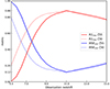 |
Fig. B.1. Metric maximum and minimum with respect to the training redshift for the validation set. The red line is for the coefficient R2 and the blue line is for the MSE. The solid lines are for ζ55 and the dashed line for ζ30 model. |
Eventually, Fig. B.2 shows the power spectrum obtained with true and predicted zreion(r) field. For ζ30, the true power spectrum is closely followed, especially at large scale. However, the smaller scales turn off faster. This effect is even worse with ζ55. For treion(r) (Fig. 12), the smaller scales turn off more efficiently, showing that small scales are more represented when working with cosmic time instead of redshift.
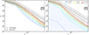 |
Fig. B.2. Power spectrum of the zreion(r) field obtained with the model ζ30 on the left and ζ55 on the right. k is the spatial frequency with dimension [cMpc−1h]. The black line stands for the ground truth and the dotted coloured lines depict predictions with different training redshifts. The shaded areas depict the dispersion around the median (1st and 99th percentiles) for both prediction and ground truth. |
The exact reason for this discrepancy is unclear. In Thélie et al. (2022b) we found that reionisation times are close to Gaussian random fields (GRFs) and can be analysed by means of GRF theory, unlike zreion(r) which is a non-linear function of treion(r). We suspect that GRFs are more easily reconstructed as they provide, for instance, a symmetric distribution of values around the mean, whereas zreion(r), for example, presents an asymetric distribution of values that is affected the most from the smoothing of extrema inherent to our implementation of CNNs.
All Tables
All Figures
|
Fig. 1. Timeline of δTb. The colour bars are in units of [mK]; ⟨δTb⟩ represents the mean of the temperature brightness. These maps come from a 21cmFAST simulation, taken at a given depth from the model ζ55 and for each redshift used in this study. White corresponds to the absence of signal, meaning that the hydrogen is ionised at this region. For this simulation, at z = 5.5, there is no neutral hydrogen anymore. Starting at z = 15, δTb is mainly seen in absorption (negative values in blue) until z = 11, where ⟨δTb⟩ becomes positive and the signal is seen in emission (positive values in red). During the whole process, HII bubbles grow with time. Figure 2 corresponds to the treion(r) associated to these maps. |
| In the text | |
|
Fig. 2. Example of 2D treion(r) map from a ζ = 55 21cmFAST model. The darker the region, the sooner it reionised. In this scenario (and for the whole ζ55 dataset), the time of reionisation of the first HII regions is approximately 0.15 Gyr (z ≈ 20, darkest spots), and the last HI regions are reionised at around 1.1 Gyr (z ≈ 5.5, brightest regions). The mean value is 0.61 Gyr (z ≈ 8.4). This treion(r) map is associated with Fig. 1, taken at the same depth in the simulation box. |
| In the text | |
|
Fig. 3. Convolutional neural network used in this work. The Encoder (left) refers to the first sequence of 2D convolutions and Max Pooling operations, while the Decoder (right) refers to the second sequence of 2D convolutions and upsampling operations. Each Max Pooling operation reduces the input map size by a factor of 2, keeping mainly large-scale information. The upsampling operator does the opposite, propagating the information at larger scales and increasing the input map size. Each convolution modifies the number of filters in such a way that we have the maximum number of filters at the deepest point of the network. Dropout and skip connection layers are depicted with black asterisks and purple arrows, respectively. Each square contains the size of the feature maps, which remain consistent along a given horizontal line (see Appendix A for additional details about the CNN model). |
| In the text | |
|
Fig. 4. Neutral fraction of hydrogen with respect to time (bottom axis) and redshift (top axis) for ζ30 (left panel) and ζ55 (right panel). The crosses stand for the average non-zero signal fraction obtained from 21 cm images at different values of z (as if taken along the line of sight). The dashed areas stand for the true QHI computed from true maps of treion(r) (mean and std). The dotted lines stand for the average QHI obtained from maps of treion(r) predicted by the CNN. |
| In the text | |
|
Fig. 5. R2 coefficient with respect to epochs for a selection of training redshifts. These curves correspond to the validation phase and are for the ζ55 model. The curves for ζ30 are not shown here, but a comparison between the two models is shown in Fig. 6. |
| In the text | |
|
Fig. 6. Metric maximum and minimum with respect to the training redshift for the validation set. The red line is for the coefficient R2 and the blue line is for the MSE. The solid lines are for ζ55 and the dashed line for ζ30 model. |
| In the text | |
|
Fig. 7. Example of prediction done by the CNN trained from images at zobs = 11 and for ζ30 model. The left panel shows the 21 cm signal δTb at this redshift. The middle panel is the ground truth of the treion field. The right panel is the CNN prediction for treion obtained from δTb (left panel). |
| In the text | |
|
Fig. 8. Examples of prediction made by the CNN trained with maps at several redshifts zobs and ζ30. The left panels show the 21 cm δTb maps. The middle column shows the predicted treion fields. The right panels show the difference TRUE-PRED. Hence, the redder it appears on the map, the more the CNN overestimates the true value at the given pixel; instead, the darker it is, the more the CNN underestimates the real value. The true treion(r) is shown in Fig. 7. |
| In the text | |
|
Fig. 9. Normalised distribution of TRUE-PRED values (as shown in Fig. 8) for several zobs. These curves were obtained from the whole test set of ζ30 models. |
| In the text | |
|
Fig. 10. True vs predicted maps obtained from the full dataset in the test set, for zobs = 11 and for both models. The red lines stand for the perfect correlation. The bottom and left histograms are the mean and the standard deviation of the residual r: r = Predicted−True, in both vertical and horizontal directions. The bottom histogram stands for the learning error, while the side histogram stands for the recovery uncertainty. In practice, the recovery uncertainty is the only accessible estimator since the ground truth will not be accessible. |
| In the text | |
|
Fig. 11. Fitting fraction with respect to redshift. The greater the allowed error for a pixel (between prediction and ground truth) is, the larger the number of pixels that have a value close to the true one within this error (i.e. ‘good pixels’). The solid lines are for ζ55 and the dotted lines for ζ30. The shaded areas depict the standard deviation around the mean for the whole predicted dataset. |
| In the text | |
|
Fig. 12. Power spectrum of the treion(r) field obtained for ζ30. k is the spatial frequency with dimension [cMpc−1 h]. The black line stands for the average power spectrum of the ground truth and the dotted coloured lines stand for P(k) predictions with different zobs. The shaded areas depict the dispersion around the median (1st and 99th percentiles) for both predictions and ground truth. |
| In the text | |
|
Fig. 13. Example of overlap map for ζ30 and a threshold value t = 0.2. The left panel is the true treion field (top) and the predicted treion(r) for a zobs of 10 (bottom). The middle panel depicts a 1 or 0 map where 1 (yellow) stands for the pixels fitting 20 % of the highest values and 0 (purple) for pixels below the threshold for the true field (top) and the predicted field (bottom). The right picture is the overlap of the middle panels, where yellow stands for coincidence, green for incorrect pixels in the prediction, and purple where the values are below the threshold in both fields. |
| In the text | |
|
Fig. 14. Dice coefficient for several zobs and for ζ30. The dashed black line stands for the Dice coefficient when matching the true map with a random mask. Pixels are considered starting with the largest pixel value (last pixel to reionise) down to a threshold. A 0.2 threshold means that we consider the last 20% to be reionised. The shaded areas depict the standard deviation around the mean DICE coefficient. |
| In the text | |
|
Fig. 15. Distribution of reionisation times for treion(r) minima. The solid line is obtained from true treion(r), while the dotted lines are obtained from predictions at several zobs. The shaded areas show the dispersion around the median (mean and std) for both predictions and ground truth. |
| In the text | |
|
Fig. 16. Predictions for the model ζ30 at zobs = 8, including instrumental effects for a typical SKA observation (left panel, see details in main text). The middle panel is the ground truth for treion(r) and the right panel is the CNN prediction. |
| In the text | |
|
Fig. 17. Power spectrum of the treion(r) field obtained with the model ζ30 at zobs = 8, including instrumental effects for a typical SKA observation. The black line and hatched area stand for the mean and standard deviation of the true field P(k). The dotted lines and shaded area depict the median and dispersion (1st and 99th percentiles) of CNN predictions P(k) with (blue) and without (red) instrumental effects. |
| In the text | |
|
Fig. 18. QHI obtained from predictions at zobs = 8 with the model ζ30, including instrumental effects for a typical SKA observation. Hatched area stands for the true field QHI. Dotted lines and shaded area depict the mean and standard deviation of CNN predictions QHI with (blue) and without (red) instrumental effects. |
| In the text | |
|
Fig. B.1. Metric maximum and minimum with respect to the training redshift for the validation set. The red line is for the coefficient R2 and the blue line is for the MSE. The solid lines are for ζ55 and the dashed line for ζ30 model. |
| In the text | |
|
Fig. B.2. Power spectrum of the zreion(r) field obtained with the model ζ30 on the left and ζ55 on the right. k is the spatial frequency with dimension [cMpc−1h]. The black line stands for the ground truth and the dotted coloured lines depict predictions with different training redshifts. The shaded areas depict the dispersion around the median (1st and 99th percentiles) for both prediction and ground truth. |
| In the text | |
Current usage metrics show cumulative count of Article Views (full-text article views including HTML views, PDF and ePub downloads, according to the available data) and Abstracts Views on Vision4Press platform.
Data correspond to usage on the plateform after 2015. The current usage metrics is available 48-96 hours after online publication and is updated daily on week days.
Initial download of the metrics may take a while.