| Issue |
A&A
Volume 672, April 2023
|
|
|---|---|---|
| Article Number | A184 | |
| Number of page(s) | 21 | |
| Section | Cosmology (including clusters of galaxies) | |
| DOI | https://doi.org/10.1051/0004-6361/202244977 | |
| Published online | 20 April 2023 | |
Topology of reionisation times: Concepts, measurements, and comparisons to Gaussian random field predictions
Université de Strasbourg, CNRS, Observatoire astronomique de Strasbourg, UMR 7550, 11 rue de l’Université, 67000 Strasbourg, France
e-mail: This email address is being protected from spambots. You need JavaScript enabled to view it.
Received:
15
September
2022
Accepted:
20
February
2023
Abstract
Context. In the next decade, radio telescopes, such as the Square Kilometer Array (SKA), will explore the Universe at high redshift, and particularly during the epoch of reionisation (EoR). The first structures emerged during this epoch, and their radiation reionised the previously cold and neutral gas of the Universe, creating ionised bubbles that percolate at the end of the EoR (z ∼ 6). SKA will produce 2D images of the distribution of the neutral gas at many redshifts, pushing us to develop tools and simulations to understand its properties.
Aims. With this paper, we aim to measure topological statistics of the EoR in the so-called reionisation time fields from both cosmological and semi-analytical simulations. This field informs us about the time of reionisation of the gas at each position; it is used to probe the inhomogeneities of reionisation histories and can be extracted from 21 cm maps. We also compare these measurements with analytical predictions obtained within Gaussian random field (GRF) theory.
Methods. The GRF theory allows us to compute many statistics of a field, namely the probability distribution functions (PDFs) of the field or its gradient, isocontour length, critical point distributions, and skeleton length. We compare these theoretical predictions to measurements made on reionisation time fields extracted from an EMMA simulation and a 21cmFAST simulation at 1 cMpc/h resolution. We also compared our results to GRFs generated from the fitted power spectra of the simulation maps.
Results. Both EMMA and 21cmFAST reionisation time fields (treion(r)) are close to being Gaussian fields, in contrast with the 21 cm, density, or ionisation fraction, which have all been shown to be non-Gaussian. Only accelerating ionisation fronts at the end of the EoR seem to be the cause of small non-gaussianities in treion(r). Overall, this topological description of reionisation times provides a new quantitative and reproducible way to characterise the EoR scenario. Under the assumption of GRFs, it enables the generation of reionisation models with their propagation, percolation, or seed statistics simply from the reionisation time power spectrum. Conversely, these topological statistics provide a means to constrain the properties of the power spectrum and by extension the physics that drive the propagation of radiation.
Key words: large-scale structure of Universe / dark ages / reionization / first stars / methods: numerical / methods: statistical / galaxies: formation / galaxies: high-redshift
© The Authors 2023
 Open Access article, published by EDP Sciences, under the terms of the Creative Commons Attribution License (https://creativecommons.org/licenses/by/4.0), which permits unrestricted use, distribution, and reproduction in any medium, provided the original work is properly cited.
This article is published in open access under the Subscribe to Open model. This email address is being protected from spambots. You need JavaScript enabled to view it. to support open access publication.
1. Introduction
The epoch of reionisation (EoR) saw the birth of stars and galaxies. Looking back at the history of the Universe, the first sources of radiation appear during the EoR, emitting photons that reionise the cosmic gas and create HII ‘bubbles’ around galaxies. These bubbles eventually percolate near the end of the EoR at z = 5.3 − 6 (Barkana & Loeb 2001; Dayal & Ferrara 2018; Kulkarni et al. 2019; Wise 2019). This epoch marks the transition from a Universe with totally cold and neutral gas to the Universe we see today, where the gas is warmer and ionised.
The evolving geometry of the EoR has been widely investigated in the literature in order to understand physical processes, such as the growth of structures, the geometry of the ionised and neutral bubbles, and the percolation process. Many works focus on the geometry of the ionised and neutral bubbles and on percolation with Minkowski functionals (or derived statistics, such as the Euler characteristic, the genus, or the shapefinders; see Gleser et al. 2006; Lee et al. 2008; Friedrich et al. 2011; Hong et al. 2014; Yoshiura et al. 2017; Chen et al. 2019; Pathak et al. 2022), with the triangle correlation function (Gorce & Pritchard 2019), or with the Morse theory and persistent homology (Thélie et al. 2022). Other studies extract the size and shape of the ionised bubbles thanks to the contour Minkowski tensor (Kapahtia et al. 2018, 2019, 2021). Counting the numbers of 3D structures in a field (isolated objects, such as peaks, tunnels, and voids) can be done using the Betti numbers (Kapahtia et al. 2019, 2021; Giri & Mellema 2021; Bianco et al. 2021; Elbers & van de Weygaert 2023). The size of the ionised or neutral bubbles has also been investigated with methods, such as the friends-of-friends algorithm (Iliev et al. 2006; Friedrich et al. 2011; Lin et al. 2016; Giri et al. 2018a, 2019), the spherical average method (Zahn et al. 2007; Friedrich et al. 2011; Lin et al. 2016; Giri et al. 2018a), the mean free path method (Mesinger & Furlanetto 2007; Lin et al. 2016; Giri et al. 2018a, 2019; Bianco et al. 2021), and the granulometry method (Kakiichi et al. 2017; Busch et al. 2020). In addition, the low-frequency component of the Square Kilometre Array radio interferometer1 (SKA-Low; see e.g. Mellema et al. 2013) will produce 2D tomographic images of the 21 cm HI emission at many redshifts during the EoR. There have therefore been many studies exploring the spatial structure of this signal, for example using the 21 cm power spectrum (Zaldarriaga et al. 2004; Furlanetto et al. 2004; McQuinn et al. 2006; Bowman et al. 2006; Lidz et al. 2008; Iliev et al. 2012; Mesinger et al. 2013; Pober et al. 2014; Greig & Mesinger 2015, 2017; Liu & Parsons 2016; Kern et al. 2017; Park et al. 2019; Pagano & Liu 2020; Gazagnes et al. 2021), or the 21 cm bispectrum (Hutter et al. 2020).
Reionisation time field: definition and motivation. Our work focuses on the reionisation time (or redshift) map. This field is generated by cosmological simulations and models (e.g. EMMA and the 21cmFAST semi-analytical code), and corresponds to the time at which each position of the simulation box is considered to be reionised, which is when the ionisation fraction exceeds a 50% threshold, as follows:
 (1)
(1)
where r is the position, and xHII is the ionised fraction.  is measured from the Big Bang, meaning that the cosmic gas is almost entirely reionised at
  Gyr. As shown in Fig. 1 and thanks to treion(r), we compress the information about the evolution of xHII into a single field instead of using a collection of snapshots. In the reionisation time map, blue regions correspond to those where the gas reionises first, whereas the red ones are the last regions where the gas reionises. We focus on 2D treion(r) maps to study the EoR on the sky as it will be observed (with the upcoming SKA 2D images for instance).
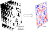 |
Fig. 1. Schematic summarising the use of the reionisation time field (on the right): it allows us to use only one field instead of a series of many snapshots of binary ionised fraction (on the left) for example. |
The field treion(r) holds both spatial and temporal information on the reionisation scenario and is therefore often used to characterise or compare the evolving structure of the reionisation provided by models. For example, it can be used to measure the speed and direction of ionising radiation as it propagates from sources (Deparis et al. 2019; Thélie et al. 2022). Recently, treion(r) was also used to efficiently generate models of the reionisation (Trac et al. 2022). This parameter is also valuable in investigations of local variations of the reionisation scenario (Trac et al. 2008; Battaglia et al. 2013; Aubert et al. 2018; Zhu et al. 2019; Sorce et al. 2022) and the consequences of an inhomogeneous reionisation. These local modulations of reionisation histories could possibly manifest themselves in the star formation histories of low-mass galaxies (Ocvirk et al. 2020) or their spatial distribution (Ocvirk & Aubert 2011). treion is therefore a versatile descriptor of models and in this paper we propose to revisit its study in a more general manner. In particular, we show how the topological study of this field can unravel many properties of the summarised reionisation scenario in a physically meaningful, quantitative, and reproducible way.
However, we also claim that this field, and the study of its topology, is not only useful in the strict and limited scope of reionisation models but also in the context of future observations. Indeed, in the next decade, radio telescopes, such as SKA, will map the intergalactic medium (IGM) during the EoR thanks to the 21 cm radiation coming from neutral hydrogen atoms (e.g. Koopmans et al. 2015). 21 cm lightcones along the line of sight will contain a wealth of information on the evolving reionisation state of the IGM and on the underlying matter density, the ionisation fraction of the gas, and its thermal state. In Hiegel et al. (in prep.), we show that it is also possible to reconstruct 2D reionisation time maps from 2D 21 cm images thanks to a convolutional neural network. Therefore, treion(r) could possibly be extracted from observations (even though small structures are smoothed out), thus granting access to the evolution of the reionisation in the transverse plane, which would complement line-of-sight studies. More details about these reconstructions are given in Appendix A. In the future, we intend to use the framework described in the present paper on the reionisation time field reconstructed from 21 cm observations.
Topology of the reionisation time field. The topological features of treion(r) can be described by analogy with a mountainous landscape (Gay 2011). Consider a mountainous landscape as a 2D field: for each 2D position of the space, the altitude is the value of the field. The mountain peaks are the maxima of the field, the bottoms of the valleys are the minima, and the mountain passes are the saddle points. The skeleton of this field corresponds to all the ridge lines, which join each of the passes (i.e. saddle points) to the peaks (i.e. maxima) and are the lines with the least slope. The skeleton forms a connected network throughout the space. With treion(r), many geometrical quantities can be interpreted physically to describe the evolution of the ionised and neutral gas during the EoR. Recently, in Thélie et al. (2022), we studied the 3D topological properties of the EoR, such as the shape, size, and orientation of ‘peak patches of reionisation’. Here, we go further and work on a large set of geometrical properties of the 2D reionisation time fields treion(r), as shown in Fig. 2.
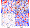 |
Fig. 2. Two-dimensional slices related to the EMMA reionisation time field that are smoothed with a Gaussian kernel with a standard deviation of Rf = 6. The top left panel shows treion(r) with its minima (black stars). The top right panel shows treion(r) with its skeleton (black lines). The bottom left panel shows the isocontours of treion(r), with its minima again in black stars. Here, the reionisation time field is normalised to put its mean at a value of 0, and its standard deviation at 1. The bottom right panel shows the norm of the gradient of treion(r). |
– Probability distribution function (PDF) of the field values. A widely used statistic when studying the EoR is the fraction of ionised volume QHII. We can measure this with the reionisation time field as it is directly the cumulated distribution function of the treion(r) values (i.e. the number of cells that has a lower reionisation time than a given threshold). In other words, it is the reionisation history; it contains information about the timing of reionisation, as well as its global evolution.
– PDF of the gradient norm field. Moreover, we can compute the first derivative of the reionisation time field, and extract the norm of its gradients. This norm corresponds to the time interval within which the gas is reionised in each cell of the simulation boxes (∼Δt/Δx), which is equivalent to the inverse of a velocity field. An example of this gradient norm field is shown in the bottom-right panel of Fig. 2. The analysis of this field allows us to study the ‘velocity’ of the radiation fronts (Deparis et al. 2019).
– Isocontour length. The isocontours of treion(r) delineate the regions reached at a given time by the HII bubbles. Their length is interesting because it contains information about the growth of the ionised bubbles and the decrease in size of the last neutral bubbles. With the bottom left panel of Fig. 2, we see the first ionised bubbles with the darkest blue contours, their growth with the lighter blue contours, and their fusion when the blue contours merge. We also see the last neutral regions being ionised with the red contours. Here, we have an insight into the percolation process of the EoR.
– Reionisation seed count. We can extract the critical points of the reionisation time field, and in particular its minima. These points correspond to the sources of radiation (first zones that reionise) and are shown on the example field of Fig. 2 with the black stars on the left panels. As expected, the critical points are within the bluest zones, which reionise first, and are also in the middle of the first blue isocontours. Their distribution as a function of time allows us to know the time of appearance of these reionisation seeds. For instance, we can infer the moment when the maximum number of sources lights up. This distribution should also correlate with the star formation rate.
– Reionisation patches. We can extract the void patches from the reionisation time field (or the peak patches from the reionisation redshift field). These patches contain all of the cells that are linked to the treion(r) minima by a negative gradient. Thanks to them, we can study the extent of the radiative influence of a reionisation seed with size distributions. Their shape and orientation with respect to the density filaments informs us about the direction of propagation of the reionisation fronts. As we studied these patches in Thélie et al. (2022), we do not focus on them in this paper.
– Distribution of the skeleton lengths. We also calculate the distribution of the length of the skeleton of treion(r). An example skeleton is shown with the black lines in the top right panel of Fig. 2. As explained before, they connect the maxima of a field by passing through its saddle points as ridge lines. The skeleton of the reionisation time field treion(r) physically corresponds to the front lines between the propagating radiation that comes from the reionisation seeds. It therefore indicates the extent to which the photons can propagate from a source and ionise the medium before reaching an opposite ionising front coming from another source: it is the percolation lines between patches of reionisation. The skeleton length distribution with respect to the time tells us about the length of merging radiation fronts at a given time.
In this work, we study all of these properties (except the reionisation patches) through measurements in treion(r) maps that are extracted from simulations obtained with the EMMA cosmological code and the 21cmFAST semi-analytical code.
Gaussianity of the reionisation time field. We also analyse the gaussianity of the reionisation time field (treion(r)), and therefore of the reionisation process. The EoR is known to be ruled by strongly non-Gaussian phenomena that are probed in different ways in the literature. Many studies look at this non-Gaussian nature of the EoR directly through the 21 cm PDF, sometimes using skewness, kurtosis, and quantile analyses (Mellema et al. 2006; Ichikawa et al. 2010; Dixon et al. 2016; Ross et al. 2019; Banet et al. 2021). Other studies use higher-order statistics, such as the bispectrum or trispectrum (Majumdar et al. 2018; Shaw et al. 2020). The density or ionisation fraction fields are also studied for their non-Gaussian features (Iliev et al. 2006). The non-gaussianities of the EoR are generally said to be due to the non-linear structure formation (Bernardeau et al. 2002), to be present at all scales, and to increase in importance as the reionisation process proceeds. Moreover, some studies show that non-gaussianities are increased within the HII bubbles due to high ionisation and high densities (Iliev et al. 2006; Dixon et al. 2016; Majumdar et al. 2018), which could be due to an inside-out process of ionisation (Iliev et al. 2006). Ross et al. (2019) also explains that the quasi-stellar objects (QSOs) and the X-ray heating can be another cause of non-gaussianity. Overall, understanding the source of non-gaussianities will help us to obtain a broader comprehension of the EoR physical processes, and to put constraints on the reionisation parameters (Shaw et al. 2020; Greig et al. 2022).
In this study, we compare the measured statistics on treion(r) mentioned above to Gaussian random field (GRF) theory predictions. This theory allows us to compute statistics of Gaussian-distributed field (Rice 1944; Longuet-Higgins 1957; Doroshkevich 1970; Bardeen et al. 1986; Hamilton et al. 1986; Pogosyan et al. 2009a,b; Pichon et al. 2010; Gay et al. 2012; Cadiou et al. 2020) or weakly non-Gaussian fields (Matsubara 2003; Pogosyan et al. 2011; Gay et al. 2012; Cadiou et al. 2020; Matsubara & Kuriki 2021). Rice (1944) first introduced the GRF theory to extract statistics from the 1D random noise of electronic devices. Longuet-Higgins (1957) later used the same theory, but this time on random waves on 2D surfaces. It is only later that Bardeen et al. (1986) used the GRF theory in astrophysics in order to study 3D structure formation in a cosmological context simply using information in a a power spectrum. More recently, Gay et al. (2012) extracted many statistics of 2D and 3D cosmological fields thanks to this theory, for example counting the peaks on synthesised cosmic microwave background (CMB) maps to study their non-gaussianities. Some widely used statistics in the context of the EoR can be analytically calculated thanks to the GRF theory, such as Minkowski functionals, the derived genus or Euler characteristics, and Betti numbers (Schmalzing & Gorski 1998; Matsubara 2003; Lee et al. 2008; Gay et al. 2012; Kapahtia et al. 2019; Matsubara & Kuriki 2021). For example, Lee et al. (2008) computed the genus of the neutral hydrogen field xHII to study the evolution of the EoR through many phases.
Here, we compare the statistics of the EoR that we measure on treion(r) with the analytic predictions of the GRF theory for the first time. The advantage of GRFs is that all of the field information is compressed within their power spectrum: we therefore envision the prospect of summarising the timing and the evolution of the EoR with treion(r) or its power spectrum. A Gaussian treion(r) has interesting applications. For example, associated evolving ionisation fields can easily be generated if we know the treion(r) power spectrum; one can imagine having a new class of fast-forward models of the reionisation process within which we could vary astrophysical parameters (that are hopefully encoded in the power spectrum of the reionisation time field). Conversely, the properties of the aforementioned topological statistics could be used to constrain the power spectrum under the GRF assumption, and by extension the physics that drives the propagation of radiation. Also, with a Gaussian treion(r), its power spectrum could be directly retrieved from measurements of its topological statistics. This could be interesting in the case where the power spectrum has not been properly measured. For instance, with the reconstructed reionisation time maps from 21 cm observations by the CNN mentioned above and in Appendix A, the power spectrum would be suppressed on small scales due the CNN smoothing, and combining the diverse statistics measured in treion(r) could help to obtain the proper power spectrum. Finally, by comparing the measurements and predictions, we show in this paper the extent to which it is realistic to suppose that treion(r) is a Gaussian field, and we also infer a few causes of non-gaussianities.
Organisation of the paper. We start by describing the EMMA and 21cmFAST simulations we used in Sect. 2, as well as some generated GRFs. Subsequently, Sect. 3 presents every topological characteristic we studied with the GRF theory. We study the behaviour of each of these characteristics with the generated GRFs, and measure them using the EMMA reionisation time fields. The same analyses are also presented for a 21cmFAST simulation in Sect. 4. In Sect. 5 we present our conclusions about this work and introduce a few perspectives. Appendix A presents some details about how we can reconstruct reionisation time maps from observation-like data. Appendix B details the calculation of the spectral moments from a specific power spectrum. Appendix C is the full calculation to obtain the PDF of the norm of the gradient of a GRF. Some results are also shown for the reionisation redshift field in order to compare it to the reionisation time field in Appendix D. The cosmology parameters used are (Ωm, Ωb, ΩΛ, h, σ8, ns) = (0.31, 0.05, 0.69, 0.68, 0.81, 0.97), as given by Planck Collaboration VI (2020).
Notations. Throughout this paper, we use the following notations, which were introduced in Pogosyan et al. (2009b), Gay et al. (2012). We use F to denote the studied field, which refers to the reionisation time fields. In this study, we work with normalised fields using the momenta of F and its derivatives:
 (2)
(2)
We introduce thereafter notations for the normalised fields and its derivatives:
 (3)
(3)
with i, j ∈ {1, 2} for 2D fields. Here, we mainly work on the reionisation time field  , which we normalise as follows:
 (4)
(4)
where  is the mean of the field. In addition, the normalised reionisation time fields are denoted x in the following work. However, when we refer to the values of the field, we use the following notation:
 (5)
(5)
As we work on normalised reionisation time fields, when ν < 0, we probe moments before the average reionisation times, and when ν > 0, we probe those after the average reionisation time. Also, low values of ν therefore refer to early reionisation times, and large values of ν to late reionisation times.
We also introduce dimensionless spectral parameters:
 (6)
(6)
These parameters can be analytically expressed if the power spectrum of the field is known. The calculation is shown in Appendix B for a specific type of power spectrum.
2. Simulated data
2.1. EMMA simulation
In this work, we used a 5123 cMpc3 h−3 cosmological simulation with a resolution of 1 cMpc3 h−3, as detailed in Gillet et al. (2021). This simulation was obtained with the cosmological code EMMA (Electromagnétisme et Mécanique sur Maille Adaptative, Aubert et al. 2015), which is an adaptive mesh refinement (AMR) code that couples hydrodynamics and radiative transfer, and in which light is described as a fluid (resolved using the moment-based M1 approximation; Aubert & Teyssier 2008). The EMMA simulation follows the cosmology given by Planck Collaboration VI (2020) and has no AMR, no reduced speed of light, and a stellar particle mass of 108 M⊙.
As this work is focused on 2D fields, 100 slices of 5122 cMpc3 h−2 in size (spaced one from another by 5 slices) are extracted from the treion(r) field. Slices are smoothed with a Gaussian kernel of standard deviation Rf ∈ {1, 2, 6} (see Sect. 2.3.2), and normalised as described in Sect. 1. The average and standard deviation of the EMMA reionisation time field are given in Table 1.
Average and standard deviation of both EMMA and 21cmFAST reionisation time and redshift fields.
2.2. 21cmFAST simulation
We compare the statistical measurements of the EMMA simulation to those of a semi-analytical simulation generated with 21cmFAST2 (version 3.0.3; Mesinger et al. 2011; Murray et al. 2020). The size of the simulation box generated is 2563 cMpc3 h−3, again with a resolution of 1 cMpc3 h−3. The reionisation model used varies by only two parameters from the default ones: the ionising efficiency of high-redshift galaxies ζ = 40, and the virial temperature Tvir = 105 K. Here, ζ controls the number of photons emitted by galaxies: the higher it is, the faster the reionisation. Tvir is the minimum virial temperature allowing a halo to start forming stars. Those parameters are chosen to approximately match the reionisation history of the 21cmFAST simulation with that of the EMMA simulation. 21cmFAST can provide us with the reionisation redshift maps that we can convert into reionisation time maps (with a given cosmology), similar to the EMMA ones. From this 3D simulation, 51 slices (of size 2562 cMpc2 h−2) can be extracted (again spaced from each other by 5 slices), and they are also smoothed and normalised the same way the EMMA slices are. The average and standard deviation of the 21cmFAST reionisation time field are given in Table 1.
2.3. Choices for the simulation data sets
2.3.1. Reionisation time and redshift fields
We also extracted the reionisation redshift fields zreion(r) from both EMMA and 21cmFAST simulations. The following statistical analyses are performed on both reionisation time and redshift fields. In the main text, we only present the results of the treion(r) field, and we briefly present a similar analysis of zreion(r) in Appendix D.
2.3.2. Smoothing
As mentioned above, we apply different smoothings on the reionisation time fields. We use Gaussian kernels with different standard deviations. We chose to smooth the fields for the following reasons:
– The future observed images from the SKA for example will have a lower spatial resolution than what we simulate here with Rf ∈ {1, 2} (see the angular resolutions given for the different kernel sizes in Table 2 compared to the equivalent values for SKA), and so SKA will not be able to probe the smallest scales of our simulations.
Angular resolutions corresponding to the size of the smoothing kernel applied to our simulation at a redshift z = 6.905.
– In order to compute the field momenta or spectral parameters, we need to integrate over power spectra, which leads to possible divergence (see the shape of the spectra in Sect. 2.4). Smoothing the fields circumvents this divergence problem, and is also well accounted for in the GRF theory.
– We use the discrete persistent structure extractor (DisPerSE3; Sousbie 2011), which assumes that the input field defines a Morse function, without large zero-gradient patches. As in Thélie et al. (2022), we use it here to extract the critical points and the skeleton of treion(r), and smoothing the field removes such patches.
– The EMMA reionisation time fields are represented in the first row of Fig. 3 for the different smoothings. The Gaussian smoothing filters out the smallest structures, while keeping the global shape of the larger scales: we ‘gaussianise’ the fields. Therefore, smoothing the reionisation time fields allows us to pinpoint the scales that are at the origin of non-Gaussian features in our measurements.
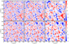 |
Fig. 3. Two-dimensional slices of the EMMA reionisation time field (first row) and the 2D GRFs obtained with the corresponding power spectrum (second row). Each column corresponds to different smoothings, with from left to right, Rf ∈ {1, 2, 6}. All the fields are normalised. |
2.4. Gaussian random fields
A GRF is a Gaussianly distributed field and if it has a null average, its PDF can be written as follows:
 (7)
(7)
where x is a n-D vector function of the position and C = ⟨x ⊗ x⟩ is the covariance matrix. For instance, x could be expressed as follows: x = (x, x1, x2, …) with the dimensionless field x = F/σ0, and its first derivatives as defined in Eq. (3).
To generate and analytically study this kind of field, we only need its power spectrum, as this defines a GRF entirely. From the power spectrum 𝒫k, we also have access to the momenta, as follows (Bardeen et al. 1986; Pogosyan et al. 2009b; Gay 2011):
 (8)
(8)
where i ∈ ℕ corresponds to the number of times the field is derivated, and d is the dimension of the field. The analytical derivation of the momenta is presented in Appendix B for a specific form of power spectrum detailed below.
We use the average power spectrum of the slices of our simulated fields: they are represented in logarithmic scales in Fig. 4 for the EMMA and 21cmFAST reionisation time fields. We use the following expression to fit these power spectra:
 (9)
(9)
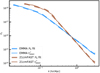 |
Fig. 4. Fitting (in dashed lines) of the reionisation time power spectra. The straight lines correspond to the power spectrum measured on the fields of each simulation (EMMA in blue and 21cmFAST in brown). The fittings are done on the average logarithmic power spectrum of every 2D slice for each field. The fields are not normalised when the fitting is carried out. |
where A1 and A2 are the amplitude of each part, and n1 and n2 are the power of each part. kthresh is the threshold separating the two parts of the power spectrum. We obtain the parameters given in Table 3 after fitting the EMMA and 21cmFAST reionisation time power spectra. In Fig. 4, the dashed lines represent the average expected power spectra in logarithmic scales of treion(r), which fit both simulations curves relatively well. This figure also demonstrates that there are more large structures in the 21cmFAST field than in the EMMA field, and also fewer small structures.
Parameters defining the power spectra of the reionisation time and redshift fields (treion(r) and zreion(r)) for both EMMA and 21cmFAST simulations.
The smoothed power spectrum of our GRF is defined as follows:
 (10)
(10)
where Rf is the standard deviation of the kernel (i.e. size of the kernel) expressed as the number of cells in the following analyses.
We also generate multiple sets of 100 runs (with different seeds) of GRFs with the power spectrum of both EMMA and 21cmFASTtreion(r) (for which, the parameters are given in the Table 3). For each power spectrum, three sets of GRFs with different smoothing are created, with the following kernel sizes: Rf ∈ {1, 2, 6}. In addition, the GRFs are all normalised the same way as the simulations. Figure 3 shows example GRF maps (second row) with different smoothing (see each column): while differences can be spotted, such GRFs are close to the EMMA fields. Figure 5 shows the expected power spectra and those measured in the simulations: the GRF and treion(r) curves are very similar. When we increase the kernel size Rf (see the purple, blue, and green curves), larger and larger scales are smoothed, as expected.
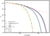 |
Fig. 5. Power spectra of the GRFs (coloured dotted lines) and EMMA reionisation times (coloured crosses). All 100 runs have been averaged to show a mean power spectrum for each set of simulations. The theoretical power spectra are shown both with and without an incorporated smoothing by the dashed and straight red lines, respectively. Three different smoothings are represented with Rf ∈ {1, 2, 6}. |
3. Topological measurements on EMMA simulations and comparisons to GRF theory predictions
In this section, we extract several topological statistics from the EMMA reionisation time field treion(r). We also derive their expression and compare them to the different runs of GRFs in order to statistically check the behaviour of our theoretical curves and our measurements.
3.1. Filling factor of the field: PDF and reionisation history
3.1.1. Measurements on the reionisation time field
The filling factor of the reionisation time field treion(r) shows the reionisation history (or fraction of ionised volume QHII) of the simulation box. This quantity allows us to study the global evolution of the ionisation of the gas during the EoR and can be directly extracted from the treion(r) map by counting the number of values lower than a time threshold, which gives us the cumulated PDF of the treion(r) values. The treion(r) PDF tells us about the distribution of reionisation times in the box: it also incorporates reionisation evolution information. If both not-cumulated and cumulated distributions are symmetric with respect to the average reionisation time, this means that the reionisation evolves in the same manner throughout the whole EoR. If they are asymmetric and if the PDF has its peak at a larger time, then reionisation begins slowly before accelerating. On the contrary, if the PDF has its peak at a smaller time, then reionisation starts rapidly before slowing down.
3.1.2. GRF theoretical expression
We can almost directly compute the filling factor of a Gaussian field with the Gaussian field theory because it only requires the PDF of the value of the field (Gay et al. 2012):
 (11)
(11)
To calculate the filling factor, the PDF only depend on the normalised field x = F/σ0. Now, this statistic is the number of field values exceeding a given threshold ν. Applied to our reionisation time fields, the number of values that are higher than a given threshold is the same as the number of cells that are still neutral. This number therefore directly corresponds to the fraction of neutral gas volume QHI. However, in our case, we are interested in the fraction of ionised volume QHII = 1 − QHI. This latter corresponds to the number of values that are lower than a given threshold, as follows:
 (12)
(12)
where  .
.
3.1.3. Comparison of the measurements and the predictions
We show the filling factors in Fig. 6 and the PDFs in Fig. 7: the crosses (and error bars) are the EMMA measurements, the dashed lines (and the shaded areas) are the GRFs measurements, and the GRF predictions are shown in black. Firstly, in both figures, the GRF distributions closely follow the predictions by the GRF theory. The filling factor measurements on the EMMA reionisation time fields are relatively close to the predictions, depicting a rather symmetric reionisation process. However, in Fig. 7, the PDFs measured on the EMMAtreion(r) maps are not symmetric, the peak being shifted towards later times; the filling factors or cumulated PDFs hide this imprint of non-gaussianity. At the same time, when we smooth the fields on larger areas (i.e. Rf increases), the distributions tend to become more symmetric around the mean reionisation time ν = 0 (i.e. close to the GRF predictions).
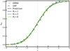 |
Fig. 6. Fraction of ionised volume for the different smoothings (in colours). The median of every run is computed for each field. The dashed lines correspond to the GRFs, and the crosses are for the EMMA reionisation time field. The black lines are the theoretical predictions. The shaded areas and the error bars represent the dispersion around the median (1st and 99th percentiles) of the GRFs and treion(r), respectively. Here, ν represents the value of the normalised reionisation times. |
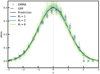 |
Fig. 7. Probability distribution function of the median of every run of the fields for the different smoothings (in colours). The dashed lines correspond to the GRFs, and the crosses are for the EMMA fields. The black lines are the theoretical predictions. The shaded areas and the error bars represent the dispersion around the median (1st and 99th percentiles) of the GRFs and treion(r), respectively. Here, ν represents the value of the normalised reionisation times. |
Therefore, the regions that ionise after the average time of the simulation (ν = 0, or around 790 Myr or a redshift of 7; see Table 1) cause the asymmetry. This means that the reionisation process is slightly slower at early times and accelerates afterwards. Mellema et al. (2006) or Dixon et al. (2016) showed that asymmetry arises towards the end of the EoR using the brightness temperature field. This asymmetry is also a key parameter in the newly developed code AMBER (Trac et al. 2022), in which we can directly tune an asymmetry parameter of the reionisation history. We see here that the non-gaussianity of the reionisation fields are filtered out with the smoothing, and are therefore hidden in the time differences on small-scale structures, and at later times.
3.2. PDF of the gradient norm field: Ionising front velocities
3.2.1. Measurements on the reionisation time field
In this section, we analyse the norm of the spatial gradients of each field that we define as follows, for a GRF or a reionisation time field F:
 (13)
(13)
where ∇ix for i ∈ {1, 2} are the two components of the gradient of the field x = F/σ0, and R0 is given in Eq. (6). Numerically, the gradients of the fields are computed thanks to Fourier transforms. Each component of the gradient is obtained as follows:
![Mathematical equation: $$ \begin{aligned} \nabla _i x = \mathcal{F} ^{-1}[\tilde{x} \times ik_i], \end{aligned} $$](/articles/aa/full_html/2023/04/aa44977-22/aa44977-22-eq23.gif) (14)
(14)
where ![Mathematical equation: $ \tilde{x} = \mathcal{F}[x] $](/articles/aa/full_html/2023/04/aa44977-22/aa44977-22-eq24.gif) is the Fourier transform of the field, and
is the Fourier transform of the field, and  . We should note that here we observe a 3D phenomenon in 2D, which means that the gradient norm is probably underestimated as we miss the third direction component of the front velocities. Figure 8 shows gradient norm maps of the reionisation time fields in the first row, and gradient norm maps of the GRFs in the second row for each smoothing (Rf ∈ {1, 2, 6}, see the columns). The two maps are relatively similar at first glance for Rf ∈ {2, 6}. However, some disparities start to be visible for the smallest smoothing kernel Rf = 1 again: the reionisation time field has larger structures than the corresponding GRF.
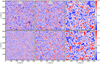 |
Fig. 8. Two-dimensional slices of the norm of the EMMA reionisation time gradient (first row) and the norm of the GRF gradient obtained with the corresponding power spectrum (second row). Each column corresponds to different smoothings, with from left to right, Rf ∈ {1, 2, 6}. |
The gradient norm of ttreion(r) is linked to the reionisation velocity field defined by Deparis et al. (2019), which is the inverse of the spatial derivative of the reionisation time field; it contains information about the ionising front velocity, and Deparis et al. (2019) showed that these fronts move forward in two stages: they are first slowed down by dense neutral gas and their speed is lower than the speed of light. However, when reaching the end of the EoR, the fronts accelerate because radiation reaches under-dense regions. This means that as time increases, the speed of the reionisation fronts increases, or conversely, the gradient norms of the reionisation time field decrease.
3.2.2. GRF theoretical expression
The PDF of the gradient norm of a Gaussian field ‖∇F‖ only depends on the field (x = F/σ0) and its first derivatives (x1 and x2 as defined in Eq. (3)), as
 (15)
(15)
This joint PDF is obtained relatively easily with Eq. (7) with a three-dimensional covariance matrix (as shown in Appendix C). From this expression, thanks to an integral over the field values and a change of variable, we can retrieve the PDF of the norm of the field gradient:
 (16)
(16)
3.2.3. Comparison of the measurements and the predictions
Firstly, the 2D distributions of the gradient norm of treion(r) with respect to the field values provide insight into the radiation front velocities at each time of the EoR. The first row of Fig. 9 shows these 2D PDFs for the EMMA reionisation time field and their corresponding GRFs are shown in second row. Each smoothing kernel size is represented with Rf ∈ {1, 2, 6} in the columns. The GRF cases are symmetric around their mean reionisation time ν = 0, as expected. We again see the asymmetry mentioned above for the EMMA reionisation time fields: the peak of the distributions is shifted towards the later times and lower velocities, especially for smaller smoothings. This asymmetry enables us to see the acceleration of the ionising fronts as the EoR progresses. If we integrate along the y-axis, we retrieve the PDF of the gradient norm, which is shown in Fig. 10. The dashed lines represent the GRF measurements, the GRF prediction is shown with the black line, and the crosses are for the EMMA reionisation time fields. The GRF measurements are superimposed on the predictions, and the EMMA measurements slightly underestimate the gradients norm because of the acceleration of the radiation fronts at the end of the EoR. On both 2D and 1D distributions, the GRF measurements are independent of the smoothing, as expected given that Eq. (15) does not depend on the kernel size. For the EMMA measurements, increasing the kernel size brings them closer to the predictions.
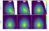 |
Fig. 9. Two-dimensional PDFs of the gradient norms with respect to the values of the fields of every run for each field and different smoothings (Rf ∈ {1, 2, 6}, see each column). The first row shows the EMMA reionisation times, and the second row their corresponding GRFs. The grey-scale lines are the isocontours of the histograms. Here, ν represents the value of the normalised reionisation times. |
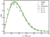 |
Fig. 10. Filling factors of the gradient norms of the fields for the different smoothings (in colours). The median of every run is computed for each field. The dashed lines correspond to the GRFs, and the crosses are for the EMMA reionisation time fields. The black lines are the theoretical predictions. The shaded areas and the error bars represent the dispersion around the median (1st and 99th percentiles) of the GRFs and treion(r), respectively. Here, w represents the value of the gradient norm of the reionisation times. |
Our measurements on the EMMA reionisation time field therefore reflect the increase in the ionising front velocities as time increases, which is probably a strong cause of the asymmetry of our reionisation time field distributions, and therefore of the non-gaussianity of the process. In any case, this phenomenon mainly impacts the small scales of treion(r) as it tends to be filtered out with large smoothing.
3.3. Isocontour length: Size evolution of ionised and neutral bubbles
3.3.1. Measurements on the reionisation time field
The isocontours of the reionisation time field tell us how far radiation propagates at a specific time. The first row of Fig. 11 shows the isocontours of the EMMA reionisation time field and the second row shows those of its corresponding GRFs. The three columns correspond to the three smoothings applied to the slices. The bluest contours represent the earliest times, and the reddest ones represent the latest times. The number of contours per level visually decreases as the size of the Gaussian kernel increases (because small structures disappear when increasing Rf).
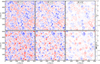 |
Fig. 11. Isocontours of 2D slices of the EMMA reionisation time field (first row) and of the 2D GRF obtained with the corresponding power spectrum (second row). Each column corresponds to a different smoothing, with Rf ∈ {1, 2, 6} from left to right. All fields are normalised. Eight levels of contours are represented with the colours. |
The isocontour length ℒ of treion(r) informs us about the extent of a reionisation time level. In Fig. 11, we can see that, as the reionisation time increases, the isocontours first encompass larger and larger regions (blue contours); when the mean reionisation time ν = 0, they begin to encompass smaller and smaller regions (red contours). Their length therefore contains information on the size of the ionised and neutral bubbles, on the percolation of the ionised bubbles, and on the different reionisation stages.
3.3.2. GRF theoretical expression
The average 2D isocontour length allows us to characterise the levels of a field by a measurement of their length; moreover, it is one of the Minkowski functionals (Schmalzing & Gorski 1998; Matsubara 2003), which have often been used to quantify the topology of the EoR (see e.g. Gleser et al. 2006; Lee et al. 2008; Friedrich et al. 2011; Hong et al. 2014; Yoshiura et al. 2017; Chen et al. 2019; Pathak et al. 2022). The isocontour length at a level ν can be defined as follows (Schmalzing & Gorski 1998; Matsubara 2003; Gay et al. 2012):
 (17)
(17)
where δ is the Dirac delta distribution; x, x1, and x2 are the normalised field and first derivatives as defined in Eq. (3);  ; and R0 is defined in Eq. (6) and corresponds to the ratio of the two first spectral momenta. This latter appears due to the normalisation of the field and its derivatives.
As ℒ depends both on the field and its first derivative, we need to use P(x, x1, x2), as defined in Eq. (15), in order to calculate it. This probability is expressed as follows:
 (18)
(18)
Now, we compute the isocontour length by integrating the quantity of Eq. (17) over the field and gradient norm values:
 (19)
(19)
3.3.3. Comparison of the measurements and the predictions
The isocontours length ℒ(ν) distributions are shown in Fig. 12 with dashed lines for the GRFs, black lines for the GRF prediction, and crosses for the EMMA reionisation time field treion(r) for the three smoothings. The measurements of the GRF distributions closely follow the GRF prediction curves, as well as the EMMA measurements. The contours grow in length until the mean reionisation time ν = 0 and then their length decreases. The measurements and predictions vary with the smoothing: the larger the Gaussian kernel, the smaller the lengths of the isocontours. Indeed, with small Rf, there are many more isocontours per reionisation level (i.e. more small structures), making a longer total length of isocontours than for large Rf.
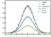 |
Fig. 12. Distribution of the isocontour length for the different smoothings (in colours). The median of every run is computed for each field. The dashed lines correspond to the GRFs, and the crosses show the EMMA reionisation time field. The black lines are the theoretical predictions. The shaded areas and the error bars represent the dispersion around the median (1st and 99th percentiles) of the GRFs and treion(r), respectively. Here, ν represents the value of the normalised reionisation times. |
As expected, the evolution of isocontour length with time traces the evolution of the ionised bubbles and neutral regions. At the beginning of the EoR, the first ionised bubbles appear because the gas starts to be ionised. These bubbles are seen as the dark blue contours in the bottom-left panel of Fig. 11. As reionisation progresses, the bubbles grow, traced by the larger contours represented by light blue levels in the same figure. The contours increase in length, and sometimes two small dark blue contours merge into one, providing insight into the percolation process. At ν ∼ 0, the isocontours have reached a maximum length, with the ionised regions intertwined with the neutral regions. Subsequently, the isocontour length ℒ decreases while the isocontours start to encompass the last neutral regions, until ℒ is close to zero at the moment when there is almost no more neutral gas. The process we mention here is very close to what Chen et al. (2019) found, namely several phases during the reionisation process, starting with an ionised bubble stage followed by an ionised fibre stage where the bubbles merge into long fibres throughout the box. Then, there is the sponge stage, which is the moment when the ionised fibres are intertwined with the neutral fibres. The process ends by a neutral fibre stage and a neutral bubble stage.
With these statistics, the EMMA reionisation times do not show significant imprints of non-gaussianities as their isocontour length follows the GRF predictions, and more so for the largest smoothing.
3.4. PDF of minima values: Reionisation seed counts
3.4.1. Measurements on the reionisation time field
In order to compare our simulations to the predicted reionisation seed count, we use the topological code DisPerSE (Sousbie 2011), which allows us to extract the critical points of a field. DisPerSE relies on the Morse theory to get topological information from the fields by studying differentiable functions. It is run on every 2D slice of reionisation time fields, as well as on every GRF generated, with a 10−5 − σ persistence threshold4.
We focus on the minima of the reionisation time field. We call these the ‘seeds’, or equivalently the ‘sources’ of reionisation because these are the first regions where the gas is locally reionised. We can measure the number of minima at a reionisation time (i.e. the PDF of the treion(r) values at its minima). Counting these reionisation seeds informs us about the evolution of the EoR: for example, if the PDF peaks at early times, the majority of the reionisation seeds appear at the beginning of the EoR, whereas if the PDF is uniformly distributed, then sources steadily contribute to reionisation throughout the whole EoR.
3.4.2. GRF theoretical expression
The PDF of the minima of the reionisation time field can also be derived with the GRF theory. To compute it, we need a joint PDF of the field that is dependent on the field, and on its first and second derivatives. Indeed, the critical points correspond to the zeros of the first derivative, and the sign of the second derivative gives us information on the type of critical point (it is positive for minima). The calculation is in six dimensions in 2D and requires changes of variables to make the covariance matrix diagonal:
 (20)
(20)
where  , and x, x11, and x22 correspond to the dimensionless field and derivatives as defined in Eq. (3). The full calculation is presented in Gay (2011) and the resulting PDF is the following:
 (21)
(21)
with
 (22)
(22)
where x1, x2, and x12 are dimensionless derivatives of the field as defined in Eq. (3).
The average extrema density is given by the following expression (which is explained in Gay 2011):
 (23)
(23)
The non-trivial part of the minima distribution calculation is the 6D integration involved in Eq. (23). A version of this integration for 3D fields is detailed in Appendix A of Bardeen et al. (1986). Additional constraints (on the eigenvalues of the hessian matrix of the field) are required to make Eq. (23) a distribution of minima. Here, we only give the resulting distribution of minima:
![Mathematical equation: $$ \begin{aligned} \begin{aligned} \frac{\partial n_{\mathrm{min}}}{\partial \nu }&= \frac{ \exp \left({\frac{-\nu ^2}{2}}\right) }{ \sqrt{2\pi }R_*^2 } \left[1 - \mathrm{erf}{ \left(\frac{\gamma \nu }{\sqrt{2(1-\gamma ^2}} \right) }\right] K_1(\nu ,\gamma ) \\&+ \frac{ \exp \left(\frac{-3\nu ^2}{6-4\gamma ^2}\right) }{ \sqrt{2\pi (1-\frac{2}{3}\gamma ^2)}R_*^2 } \left[1 - \mathrm{erf}{ \left(\frac{\gamma \nu }{\sqrt{2(1-\gamma ^2)(3-2\gamma ^2)}} \right)} \right] K_2 \\&- \frac{ \exp \left(\frac{-\nu ^2}{2(1-\gamma ^2)}\right) }{ \sqrt{2\pi (1-\gamma ^2)}R_*^2 } \left[1 + \exp \left( \frac{\nu ^2}{2(1-\gamma ^2)} \right) \right] K_3(\nu ,\gamma ), \\ \end{aligned} \end{aligned} $$](/articles/aa/full_html/2023/04/aa44977-22/aa44977-22-eq37.gif) (24)
(24)
where R* is defined in Eq. (6), and
 (25)
(25)
3.4.3. Comparison of the measurements and the predictions
The PDFs of the minima values are shown in Fig. 13, with dashed lines showing the GRFs, full black lines the predictions, and crosses the EMMA reionisation time field. The three smoothings are represented (see the three Rf values in different colours). The theoretical PDFs are centred around early reionisation times (i.e. ν < 0) because we look for minima. The GRFs and EMMAtreion(r) fields closely follow the expected curves. When the fields are smoothed with a larger kernel (increasing Rf), the least significant minima get smoothed out, decreasing the number of counted minima. We also note that smoothing on larger areas causes the distributions to be shifted towards smaller values of the field (i.e. towards the beginning of the EoR).
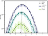 |
Fig. 13. Distribution of the critical points of the fields for the different smoothings (in colours). The median of every run is computed for each field. The dashed lines correspond to the GRFs, and the crosses are for the EMMA reionisation time fields. The black lines are the theoretical predictions. The shaded areas and the error bars represent the dispersion around the median (1st and 99th percentiles) of the GRFs and treion(r), respectively. The black dotted vertical lines represent the average of the predictions. Here, ν represents the value of the normalised reionisation times. |
With these results, we can see that when the EoR begins (smallest ν), there are a few reionisation seeds that represent the first radiation sources of the Universe. The further the reionisation progresses, the more the number of reionisation seeds increases as more and more galaxies are created. This number continues to increase until some intermediate time, where the minima distributions peak, which happens before the average reionisation time at the mean reionisation time ν = 0. The distributions then decrease because more and more intergalactic gas is reionised by the already existing radiation sources, until it is all reionised. At this time, no more new seeds of ionisation front propagation appear, although there can be new sources in already reionised places. The impact of the smoothing is that only the most exceptional and early reionisation seeds remain in the smoothed fields – because they are sufficiently significant –, while the other ones are filtered out. This means that these exceptional seeds reionise the other ones in an inside-out way. Globally, there is little to no imprint of non-gaussianities with this statistic within the error bars.
3.5. Skeleton length: Regions of ionising front percolation
3.5.1. Measurements on the reionisation time field
Thanks to DisPerSE, we can also extract the skeleton of treion(r) from every reionisation time field and GRF using the same persistence value as in Sect. 3.4. The skeleton is, as explained in Sect. 1, the network formed by all the segments joining the maxima and saddle points together along the ridge of the field. In 2D, the skeleton corresponds to the edges of the reionisation patches, which are regions under the radiative influence of a reionisation seed. These edges, or the place where the patches intersect, are also the front lines between the radiation fronts of reionisation. Looking at the skeleton (in black) in the top right panel of Fig. 2, we can see that it seems to be preferentially aligned diagonally on the map, which is due to diamond shapes produced around sources that are caused by the M1 approximation used in EMMA to model the radiative transfer (Aubert & Teyssier 2008).
We are interested in the length distribution of the skeleton as a function of time. As an example, if the distributions are as narrow as a Dirac distribution, then the reionisation seeds are uniformly distributed in space, which in turn means that all the radiation fronts encounter opposite fronts all at the same time. If the Dirac distribution peaks at ν < 0, then the percolation happens at early times, and if it peaks at ν > 0, then the percolation happens at late times. Otherwise, if the distribution is wider, the seeds are not uniformly distributed and the merger of the reionisation patches happens throughout the reionisation process. If there were many ionised bubbles at early times and then a single growing bubble, then the distribution would be asymmetric. As the skeleton is the place where radiation fronts meet, it is impacted by the front velocities: if the fronts propagate faster, they can reach more-distant regions, meaning that the reionisation patches are larger. If ones assumes a simple 2D lattice of circular patches of radius R, it is expected to have a total skeleton length per unit surface of L ∼ 2πR/πR2 ∼ R−1; a scenario with large patches should lead to small L values. Also, the accelerated fronts can cause the percolation to happen more rapidly in the remaining neutral regions, causing the distribution to decrease more sharply at the end of the EoR, and to therefore be asymmetric with respect to time. Generally speaking, these distributions tell us whether the ionising fronts percolate in a longer or shorter period of time.
3.5.2. GRF theoretical expression
The analytical calculation of the skeleton-length distribution has been described by several authors, such as Pogosyan et al. (2009b), Gay (2011), Gay et al. (2012). The calculations are presented in detail by Pogosyan et al. (2009b) for example. In summary, the skeleton corresponds to all the points for which the gradient is aligned with an eigenvector of the hessian of the field, ℋ = ∇∇F, following the gradient in the direction of the positive eigenvalue of the hessian5. This definition can be mathematically written as follows: ℋ ⋅ ∇F = λ∇F, where λ is the positive eigenvalue of the hessian. In an equivalent way, a point is on a critical line if s = det(ℋ ⋅ ∇x, λ⃗∇x) = 0, with the dimensionless field x (=F/σ0). The skeleton-length distribution can therefore be written as follows:
 (26)
(26)
with |∇s| giving the length of the critical lines, and R* given in Eq. (6). The integration of Eq. (26) involves the PDF of the field, and its first, second, and third derivative. The ‘stiff approximation’ allows us to neglect the derivatives of higher than third order, which simplifies the calculations. The critical lines are therefore considered to be relatively straight: the total length of the skeleton may therefore probably be reduced with this approximation. The final expression of the skeleton length per unit of the total field surface is therefore
![Mathematical equation: $$ \begin{aligned} \begin{aligned} \frac{\partial L^\mathrm{skel}}{\partial \nu }&= \frac{1}{\sqrt{2\pi } R_*} \exp ^{-\frac{\nu ^2}{2}} \Biggr [ \frac{1}{8\sqrt{\pi }} (\sqrt{\pi } + 2 \gamma \nu ) \left( 1 + \mathrm{erf}\left( \frac{\gamma \nu }{\sqrt{2(1-\gamma ^2)}} \right) \right) \\&+ \frac{\sqrt{1-\gamma ^2}}{2\sqrt{2}\pi } \exp \left( - \frac{\gamma ^2\nu ^2}{2(1-\gamma ^2} \right) \Biggr ], \\ \end{aligned} \end{aligned} $$](/articles/aa/full_html/2023/04/aa44977-22/aa44977-22-eq40.gif) (27)
(27)
with γ defined in Eq. (6).
The total skeleton length of a field can be obtained by integrating the distribution of Eq. (27) over all values of ν. The resulting expression is (Pogosyan et al. 2009b; Gay 2011)
 (28)
(28)
3.5.3. Comparison of the measurements and the predictions
The skeleton-length PDFs are shown in Fig. 14 with dashed lines for the GRFs, full black lines for the predictions, and crosses for the EMMA reionisation time field. The colours represent the three different smoothings (see the three Rf values in different colours). The ‘stiff approximation’ leads to discrepancies between the measurements and the predictions. In addition, the analytical calculation of the skeleton length is local and DisPerSE gives a global skeleton (Pogosyan et al. 2009b; Gay et al. 2012), meaning that the predictions tend to underestimate the skeleton length by probably missing filaments. For these reasons, we multiply our measurements by a normalisation factor6 to match the prediction amplitude following Gay et al. (2012). Still, the shape of the distributions seems to be conserved, as the renormalised measurements on the GRFs are almost perfectly superimposed on the predicted curves. The measurements on the reionisation time fields from EMMA are also relatively close to the predictions, especially when increasing Rf. The PDFs increase until reaching a maximum after the average reionisation time (ν > 0), before decreasing again. They are not centred on the average reionisation time ν = 0; instead they are shifted to later times when the smoothings increase, and are asymmetric, except for the highest smoothings (Rf = 6), for which the measured EMMA distributions are ‘symmetrised’ thanks to the smoothing, and therefore closer to the predictions.
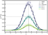 |
Fig. 14. Distribution of the skeleton length of the fields for the different smoothings (in colours). The median of every run is computed for each field. The dashed lines correspond to the GRFs, and the crosses are for the EMMA reionisation time fields. The black lines are the theoretical predictions. The shaded areas and the error bars represent the dispersion around the median (1st and 99th percentiles) of the GRFs and treion(r), respectively. The black dotted vertical lines represent the average of the predictions. Here, ν represents the value of the normalised reionisation times. |
With this statistic, we can again follow the evolution of the EoR from the point of view of merging radiation fronts. During the first stages of the EoR, the ionised bubbles grow, and the radiation fronts start to reach farther out, increasing the skeleton length. At a reionisation time of ν > 0, the distribution peaks when the ionising fronts percolate on the longer length; at this moment there are large ionised fibres. Subsequently, most gas is reionised, and there is less percolation of ionised bubbles, meaning that fewer ionised fronts encounter other fronts, until the gas is totally ionised at the end of the EoR (ν ∼ 3 as in the reionisation history). With small smoothing kernel sizes (Rf ∈ {1, 2}), we retrieve the asymmetry that results from the increase in the radiation front velocities at the end of the EoR, as expected.
4. Predictions from Gaussian random field theories compared to 21cmFAST simulations
In this section, we compare the theoretical statistics described in Sect. 3 to the 21cmFAST reionisation time field. For the sake of brevity, we only show the 2D histograms of the field values and its gradient norms, the fraction of the ionised volume of gas, and the skeleton length distribution for the 21cmFAST reionisation time fields and the GRFs generated with the corresponding power spectrum. Indeed, the 21cmFAST reionisation fields give similar results to the EMMA ones: the semi-analytical generated field is generally close to the GRF predictions. This latter field depicts an almost Gaussian behaviour in every statistic and smoothing studied in this paper, as for the EMMA simulation, albeit slightly less Gaussian for the minima and skeleton length distributions. Again, increasing the Gaussian kernel size (i.e. increasing Rf) tends to ‘gaussianise’ the reionisation time field.
The first row of Fig. 15 shows the 2D histograms for treion(r) and the second row shows the GRFs. Each column represents a different Gaussian smoothing with Rf ∈ {1, 2, 6}, respectively. Figure 16 shows the fraction of ionised volume, and Fig. 17 shows the PDF of the skeleton length. Both figures show the GRF predictions in black, the 21cmFAST reionisation time fields in coloured crosses, and the GRF measurements in coloured dashed lines. In the 21cmFAST field, there are more imprints of non-gaussianities: the gradient norms decrease dramatically at higher times (i.e. the front velocities increase dramatically). This decrease was already the case in the EMMA simulation, but it is much more pronounced in the present case. For the two smallest smoothings, this non-gaussianity imprint also appears in the QHII statistic (see Fig. 16), where the gas seems to be totally reionised earlier than in the predictions or in the skeleton length PDFs (see Fig. 17), where at later times, the distributions depart from the predictions. Moreover, 21cmFAST does not explicitly model radiation propagation (Zahn et al. 2011), which means that the front velocities are not limited by the speed of light, for example. This is not the case in EMMA, and could explain the small gradient values at late times.
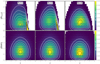 |
Fig. 15. Two-dimensional PDFs of the gradient norms with respect to the values of the fields of every run for each field and different smoothings (Rf ∈ {1, 2, 6}, see each column). The first row corresponds to the 21cmFAST reionisation times, and the second row to their corresponding GRFs. The grey-scale lines are the isocontours of the histograms. Here, ν represents the value of the normalised reionisation times. |
Nevertheless, even if the 21cmFAST measurements of Figs. 16 and 17 are not superimposed on the predictions, they remain within the measurement error bars. For the two smallest smoothing kernels, the 21cmFAST skeleton length distributions (Fig. 17) peak at a lower skeleton length value than the EMMA distributions (Fig. 14). This means that at a given time, the skeleton lengths are smaller in the 21cmFAST simulation than in the EMMA simulation: there are less percolation places in the 21cmFAST simulation than in the EMMA simulation at a given moment. As already mentioned, a shorter skeleton length implies larger patches for a simple lattice model; this would be consistent with the results obtained in Thélie et al. (2022), where 21cmFAST patches were usually found to be larger than the ones found in the EMMA simulation for similar models.
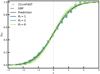 |
Fig. 16. Fraction of ionised volume of the fields for the different smoothings (in colours). The median of every run is computed for each field. The dashed lines correspond to the GRFs, and the crosses are for the 21cmFAST reionisation time fields. The black lines are the theoretical predictions. The shaded areas and the error bars represent the dispersion around the median (1st and 99th percentiles) of the GRFs and treion(r), respectively. Here, ν represents the value of the normalised reionisation times. |
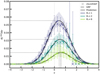 |
Fig. 17. Distribution of the skeleton length of the fields for the different smoothings (in colours). The median of every run is computed for each field. The dashed lines correspond to the GRFs, and the crosses are for the 21cmFAST reionisation time fields. The black lines are the theoretical predictions. The shaded areas and the error bars represent the dispersion around the median (1st and 99th percentiles) of the GRFs and treion(r), respectively. The black dotted vertical lines represent the average of the predictions. Here, ν represents the value of the normalised reionisation times. |
5. Conclusion and perspectives
In this work, we extract topological statistics from 2D reionisation time (and redshift in Appendix D) maps produced based on an EMMA cosmological simulation and on a 21cmFAST semi-analytical simulation (which have approximately the same reionisation history). Reionisation time maps contain a wealth of spatial and temporal information about the reionisation process. The fraction of ionised volume (i.e. the filling factor of the treion(r) map) contains information on the global timing and evolution of the reionisation process. The PDF of the gradient norm map informs us about the velocity of the radiation fronts. The average isocontour length of the field allows us to follow the percolation process. The critical point distributions inform us about the timing of the appearance of reionisation seeds. The skeleton lengths tell us about the moment, duration, and place of the percolation of ionisation fronts. We also apply the GRF theory (Rice 1944; Longuet-Higgins 1957; Doroshkevich 1970; Bardeen et al. 1986; Gay et al. 2012) in the context of the EoR to compare GRF predictions to measurements of these statistics in simulations. We generate GRFs from a fitted power spectrum of each simulation to check our simulation measurements.
We show that the topological statistics extracted from the EMMA and 21cmFAST reionisation time maps are relatively close to the GRF predictions, and are even closer when the maps are smoothed on larger areas. This means that treion(r) can be assumed to be Gaussian with a good level of approximation, and that we have therefore developed a simple tool that allows us to quickly generate fields related to reionisation. This result is surprising in a context where many other EoR fields have been shown to be highly non-Gaussian, such as the 21 cm or the density fields (see e.g. Mellema et al. 2006; Iliev et al. 2006; Majumdar et al. 2018; Ross et al. 2019). We find the major differences between the EMMA cosmological simulation and the 21cmFAST semi-analytical simulation reionisation time fields to be caused by the increase in the velocity of the fronts at the end of the EoR.
The topological statistics applied to the reionisation time field can therefore be used to characterise the evolution of the EoR. The reasonable agreement between GRF predictions and model measurements also suggests that it may be possible to generate histories of reionisation on the sky from the simple knowledge of the power spectrum of the reionisation time field. Such generated histories would automatically come with a set of topological statistics (number of reionisation seeds, skeleton length, Minkowski functionals, etc.) fully determined by the power spectrum within the framework of GRF theory. In addition, we show here that the reionisation evolution can be inferred from the power-spectrum parameters (or the spectral parameters R0, R*, and γ) only, as long as the scales are sufficiently large for the reionisation time field to be close to a GRF. Finally, the topological statistics discussed here directly depend on the power-spectrum parameters (amplitudes, slopes, characteristic scales) in the GRF approximation. The physics of the propagation of reionisation, which is presumably encoded in the power spectrum, can be constrained even in situations where the power spectrum cannot be easily estimated, for example by fitting peaks, isocontours, or skeleton statistics with their Gaussian predictions. As such, these statistics can be used to constrain the power spectrum, even in situations where the reionisation time fields suffer from noise or poor resolution, for example.
However, our studies show that this similarity with GRF predictions operates on large scales of about 8 cMpc/h, which is similar to the SKA resolution at these redshifts. We still see small imprints of non-gaussianities on the smaller scales. Indeed, at the end of the EoR, the radiation fronts propagate increasingly quickly because of the remaining neutral voids. This velocity increase makes the process asymmetric with respect to the mean reionisation time, and it is poorly reconstructed with the symmetric theory that is the GRF theory. As the regions that remain to be ionised decrease in size as the EoR comes to an end, this phenomenon remains at small scales, and the velocity increase gets smoothed out with the largest smoothing. To take these asymmetries into account, we could add non-Gaussian terms in our expressions with the Gram-Charlier expansion (Gay et al. 2012; Cadiou et al. 2020). Also, it could be interesting to investigate how reduced-speed-of-light approximations (Deparis et al. 2019; Ocvirk et al. 2019) influence the statistics presented here and could lead to an even better agreement with GRF predictions. In any case, our results are probably resolution-dependent and we could verify this with models of higher resolution.
Finally, the reionisation time or redshift fields are not directly observable. In the next decade, the SKA observatory will provide 21 maps of the EoR that will be of similar resolution to our simulation smoothed with Rf = 6. For this reason, we are creating a method to be presented in a future paper (Hiegel et al., in prep.) to reconstruct 2D reionisation redshift maps from 2D 21 cm maps (that are taken at a given redshift), and from which we can compute the reionisation time maps. With these maps, we will be able to infer the topological characteristics of the reionisation process as we do here with simulations.
The value of the persistence parameter chosen here is very low in order to apply no selection on the extracted critical points. It is a threshold controlling the maximal distance between the field values in a maximum–minimum pair within the extracted features by DisPerSE. The persistence allows us to control the significance of the extracted topological features, and therefore the smoothness of the features. It can be used to override the noise of the input field. More details are given by Sousbie (2011) or Thélie et al. (2022).
Returning to our representation of the topology through a mountain landscape, the skeleton, and therefore the ridge lines, are referred to as critical lines in topology. Walking on a ridge line is coming from a pass and going in the direction that goes up to the peak: this means that we follow the gradient in the direction of the positive eigenvalue of the hessian. In addition, we note that, if we were to follow the gradient in the direction of the negative eigenvalue of the hessian, we would be on the anti-skeleton, aiming at reaching a minima.
The normalisation factor is given by the ratio between the total length of the measured skeleton over the one of the prediction. It depends on the smoothing via the spectral parameter R* (see Eq. (28)).
Acknowledgments
We thank Christophe Pichon and Corentin Cadiou for their help and advice on the understanding of the GRF theory. This work was granted access to the HPC resources of CINES and TGCC under the allocations 2020-A0070411049, 2021- A0090411049, and 2022-A0110411049 “Simulation des signaux et processus de l’aube cosmique et Réionisation de l’Univers” made by GENCI. This research made use of TOOLS21CM, a community-developed package for the analysis of the 21 cm signals from the EoR and Cosmic Dawn (Giri et al. 2020), ASTROPY, a community-developed core Python package for astronomy (Astropy Collaboration 2018); MATPLOTLIB, a Python library for publication quality graphics (Hunter 2007); SCIPY, a Pythonbased ecosystem of open-source software for mathematics, science, and engineering (Virtanen et al. 2020); NUMPY (Harris et al. 2020) and IPYTHON (Perez & Granger 2007).
References
- Astropy Collaboration (Price-Whelan, A. M., et al.) 2018, AJ, 156, 123 [Google Scholar]
- Aubert, D., & Teyssier, R. 2008, MNRAS, 387, 295 [NASA ADS] [CrossRef] [Google Scholar]
- Aubert, D., Deparis, N., & Ocvirk, P. 2015, MNRAS, 454, 1012 [Google Scholar]
- Aubert, D., Deparis, N., Ocvirk, P., et al. 2018, ApJ, 856, L22 [Google Scholar]
- Banet, A., Barkana, R., Fialkov, A., & Guttman, O. 2021, MNRAS, 503, 1221 [NASA ADS] [CrossRef] [Google Scholar]
- Bardeen, J. M., Bond, J. R., Kaiser, N., & Szalay, A. S. 1986, ApJ, 304, 15 [Google Scholar]
- Barkana, R., & Loeb, A. 2001, Phys. Rep., 349, 125 [NASA ADS] [CrossRef] [Google Scholar]
- Battaglia, N., Trac, H., Cen, R., & Loeb, A. 2013, ApJ, 776, 81 [NASA ADS] [CrossRef] [Google Scholar]
- Bernardeau, F., Colombi, S., Gaztañaga, E., & Scoccimarro, R. 2002, Phys. Rep., 367, 1 [Google Scholar]
- Bianco, M., Giri, S. K., Iliev, I. T., & Mellema, G. 2021, MNRAS, 505, 3982 [NASA ADS] [CrossRef] [Google Scholar]
- Bowman, J. D., Morales, M. F., & Hewitt, J. N. 2006, ApJ, 638, 20 [NASA ADS] [CrossRef] [Google Scholar]
- Busch, P., Eide, M. B., Ciardi, B., & Kakiichi, K. 2020, MNRAS, 498, 4533 [NASA ADS] [CrossRef] [Google Scholar]
- Cadiou, C., Pichon, C., Codis, S., et al. 2020, MNRAS, 496, 4787 [Google Scholar]
- Chen, Z., Xu, Y., Wang, Y., & Chen, X. 2019, ApJ, 885, 23 [NASA ADS] [CrossRef] [Google Scholar]
- Dayal, P., & Ferrara, A. 2018, Phys. Rep., 780, 1 [Google Scholar]
- Deparis, N., Aubert, D., Ocvirk, P., Chardin, J., & Lewis, J. 2019, A&A, 622, A142 [NASA ADS] [CrossRef] [EDP Sciences] [Google Scholar]
- Dixon, K. L., Iliev, I. T., Mellema, G., Ahn, K., & Shapiro, P. R. 2016, MNRAS, 456, 3011 [NASA ADS] [CrossRef] [Google Scholar]
- Doroshkevich, A. G. 1970, Astrophysics, 6, 320 [Google Scholar]
- Elbers, W., & van de Weygaert, R. 2023, MNRAS, 520, 2709 [NASA ADS] [CrossRef] [Google Scholar]
- Friedrich, M. M., Mellema, G., Alvarez, M. A., Shapiro, P. R., & Iliev, I. T. 2011, MNRAS, 413, 1353 [NASA ADS] [CrossRef] [Google Scholar]
- Furlanetto, S. R., Zaldarriaga, M., & Hernquist, L. 2004, ApJ, 613, 16 [NASA ADS] [CrossRef] [Google Scholar]
- Gay, C. 2011, Ph.D. Thesis, thèse de doctorat en Physique dirigée par Christophe Pichon, Paris [Google Scholar]
- Gay, C., Pichon, C., & Pogosyan, D. 2012, Phys. Rev. D, 85, 023011 [NASA ADS] [CrossRef] [Google Scholar]
- Gazagnes, S., Koopmans, L. V. E., & Wilkinson, M. H. F. 2021, MNRAS, 502, 1816 [NASA ADS] [CrossRef] [Google Scholar]
- Gillet, N. J. F., Aubert, D., Mertens, F. G., & Ocvirk, P. 2021, ArXiv e-prints [arXiv:2103.03061] [Google Scholar]
- Giri, S. K., & Mellema, G. 2021, MNRAS, 505, 1863 [NASA ADS] [CrossRef] [Google Scholar]
- Giri, S. K., Mellema, G., Dixon, K. L., & Iliev, I. T. 2018a, MNRAS, 473, 2949 [NASA ADS] [CrossRef] [Google Scholar]
- Giri, S. K., Mellema, G., & Ghara, R. 2018b, MNRAS, 479, 5596 [NASA ADS] [CrossRef] [Google Scholar]
- Giri, S. K., Mellema, G., Aldheimer, T., Dixon, K. L., & Iliev, I. T. 2019, MNRAS, 489, 1590 [NASA ADS] [CrossRef] [Google Scholar]
- Giri, S., Mellema, G., & Jensen, H. 2020, J. Open Source Softw., 5, 2363 [NASA ADS] [CrossRef] [Google Scholar]
- Gleser, L., Nusser, A., Ciardi, B., & Desjacques, V. 2006, MNRAS, 370, 1329 [NASA ADS] [CrossRef] [Google Scholar]
- Gorce, A., & Pritchard, J. R. 2019, MNRAS, 489, 1321 [NASA ADS] [CrossRef] [Google Scholar]
- Greig, B., & Mesinger, A. 2015, MNRAS, 449, 4246 [NASA ADS] [CrossRef] [Google Scholar]
- Greig, B., & Mesinger, A. 2017, MNRAS, 472, 2651 [NASA ADS] [CrossRef] [Google Scholar]
- Greig, B., Ting, Y.-S., & Kaurov, A. A. 2022, MNRAS, 513, 1719 [NASA ADS] [CrossRef] [Google Scholar]
- Hamilton, A. J. S., Gott, J., Richard, I., & Weinberg, D. 1986, ApJ, 309, 1 [NASA ADS] [CrossRef] [Google Scholar]
- Harris, C. R., Millman, K. J., van der Walt, S. J., et al. 2020, Nature, 585, 357 [NASA ADS] [CrossRef] [Google Scholar]
- Hong, S. E., Ahn, K., Park, C., et al. 2014, J. Korean Astron. Soc., 47, 49 [NASA ADS] [CrossRef] [Google Scholar]
- Hunter, J. D. 2007, Comput. Sci. Eng., 9, 90 [NASA ADS] [CrossRef] [Google Scholar]
- Hutter, A., Watkinson, C. A., Seiler, J., et al. 2020, MNRAS, 492, 653 [CrossRef] [Google Scholar]
- Ichikawa, K., Barkana, R., Iliev, I. T., Mellema, G., & Shapiro, P. R. 2010, MNRAS, 406, 2521 [NASA ADS] [CrossRef] [Google Scholar]
- Iliev, I. T., Mellema, G., Pen, U. L., et al. 2006, MNRAS, 369, 1625 [NASA ADS] [CrossRef] [Google Scholar]
- Iliev, I. T., Mellema, G., Shapiro, P. R., et al. 2012, MNRAS, 423, 2222 [NASA ADS] [CrossRef] [Google Scholar]
- Kakiichi, K., Majumdar, S., Mellema, G., et al. 2017, MNRAS, 471, 1936 [NASA ADS] [CrossRef] [Google Scholar]
- Kapahtia, A., Chingangbam, P., Appleby, S., & Park, C. 2018, J. Cosmol. Astropart. Phys., 2018, 011 [CrossRef] [Google Scholar]
- Kapahtia, A., Chingangbam, P., & Appleby, S. 2019, J. Cosmol. Astropart. Phys., 2019, 053 [CrossRef] [Google Scholar]
- Kapahtia, A., Chingangbam, P., Ghara, R., Appleby, S., & Choudhury, T. R. 2021, J. Cosmol. Astropart. Phys., 2021, 026 [CrossRef] [Google Scholar]
- Kern, N. S., Liu, A., Parsons, A. R., Mesinger, A., & Greig, B. 2017, ApJ, 848, 23 [NASA ADS] [CrossRef] [Google Scholar]
- Koopmans, L., Pritchard, J., Mellema, G., et al. 2015, Advancing Astrophysics with the Square Kilometre Array (AASKA14), 1 [Google Scholar]
- Kulkarni, G., Keating, L. C., Haehnelt, M. G., et al. 2019, MNRAS, 485, L24 [Google Scholar]
- Lee, K.-G., Cen, R., Gott, J., Richard, I., & Trac, H. 2008, ApJ, 675, 8 [NASA ADS] [CrossRef] [Google Scholar]
- Lidz, A., Zahn, O., McQuinn, M., Zaldarriaga, M., & Hernquist, L. 2008, ApJ, 680, 962 [NASA ADS] [CrossRef] [Google Scholar]
- Lin, Y., Oh, S. P., Furlanetto, S. R., & Sutter, P. M. 2016, MNRAS, 461, 3361 [NASA ADS] [CrossRef] [Google Scholar]
- Liu, A., & Parsons, A. R. 2016, MNRAS, 457, 1864 [NASA ADS] [CrossRef] [Google Scholar]
- Longuet-Higgins, M. S. 1957, Philos. Trans. R. Soc. London Ser. A Math. Phys. Sci., 249, 321 [NASA ADS] [Google Scholar]
- Majumdar, S., Pritchard, J. R., Mondal, R., et al. 2018, MNRAS, 476, 4007 [NASA ADS] [CrossRef] [Google Scholar]
- Matsubara, T. 2003, ApJ, 584, 1 [NASA ADS] [CrossRef] [Google Scholar]
- Matsubara, T., & Kuriki, S. 2021, Phys. Rev. D, 104, 103522 [NASA ADS] [CrossRef] [Google Scholar]
- McQuinn, M., Zahn, O., Zaldarriaga, M., Hernquist, L., & Furlanetto, S. R. 2006, ApJ, 653, 815 [NASA ADS] [CrossRef] [Google Scholar]
- Mellema, G., Iliev, I. T., Pen, U.-L., & Shapiro, P. R. 2006, MNRAS, 372, 679 [NASA ADS] [CrossRef] [Google Scholar]
- Mellema, G., Koopmans, L. V. E., Abdalla, F. A., et al. 2013, Exp. Astron., 36, 235 [NASA ADS] [CrossRef] [Google Scholar]
- Mesinger, A., & Furlanetto, S. 2007, ApJ, 669, 663 [Google Scholar]
- Mesinger, A., Furlanetto, S., & Cen, R. 2011, MNRAS, 411, 955 [Google Scholar]
- Mesinger, A., Ferrara, A., & Spiegel, D. S. 2013, MNRAS, 431, 621 [NASA ADS] [CrossRef] [Google Scholar]
- Murray, S., Greig, B., Mesinger, A., et al. 2020, J. Open Source Softw., 5, 2582 [NASA ADS] [CrossRef] [Google Scholar]
- Ocvirk, P., & Aubert, D. 2011, MNRAS, 417, L93 [NASA ADS] [CrossRef] [Google Scholar]
- Ocvirk, P., Aubert, D., Chardin, J., Deparis, N., & Lewis, J. 2019, A&A, 626, A77 [NASA ADS] [CrossRef] [EDP Sciences] [Google Scholar]
- Ocvirk, P., Aubert, D., Sorce, J. G., et al. 2020, MNRAS, 496, 4087 [NASA ADS] [CrossRef] [Google Scholar]
- Pagano, M., & Liu, A. 2020, MNRAS, 498, 373 [NASA ADS] [CrossRef] [Google Scholar]
- Park, J., Mesinger, A., Greig, B., & Gillet, N. 2019, MNRAS, 484, 933 [NASA ADS] [CrossRef] [Google Scholar]
- Pathak, A., Bag, S., Dasgupta, S., et al. 2022, J. Cosmol. Astropart. Phys., 2022, 027 [CrossRef] [Google Scholar]
- Perez, F., & Granger, B. E. 2007, Comput. Sci. Eng., 9, 21 [Google Scholar]
- Pichon, C., Gay, C., Pogosyan, D., et al. 2010, in AIP Conf. Ser., eds. J. M. Alimi, & A. Fuözfa, 1241, 1108 [Google Scholar]
- Planck Collaboration VI. 2020, A&A, 641, A6 [NASA ADS] [CrossRef] [EDP Sciences] [Google Scholar]
- Pober, J. C., Liu, A., Dillon, J. S., et al. 2014, ApJ, 782, 66 [NASA ADS] [CrossRef] [Google Scholar]
- Pogosyan, D., Gay, C., & Pichon, C. 2009a, Phys. Rev. D, 80, 081301 [NASA ADS] [CrossRef] [Google Scholar]
- Pogosyan, D., Pichon, C., Gay, C., et al. 2009b, MNRAS, 396, 635 [NASA ADS] [CrossRef] [Google Scholar]
- Pogosyan, D., Pichon, C., & Gay, C. 2011, Phys. Rev. D, 84, 083510 [NASA ADS] [CrossRef] [Google Scholar]
- Rice, S. O. 1944, Bell Syst. Tech. J., 23, 282 [NASA ADS] [CrossRef] [Google Scholar]
- Ross, H. E., Dixon, K. L., Ghara, R., Iliev, I. T., & Mellema, G. 2019, MNRAS, 487, 1101 [NASA ADS] [CrossRef] [Google Scholar]
- Schmalzing, J., & Gorski, K. M. 1998, MNRAS, 297, 355 [CrossRef] [Google Scholar]
- Shaw, A. K., Bharadwaj, S., & Mondal, R. 2020, MNRAS, 498, 1480 [CrossRef] [Google Scholar]
- Sorce, J. G., Ocvirk, P., Aubert, D., et al. 2022, MNRAS, 515, 2970 [NASA ADS] [CrossRef] [Google Scholar]
- Sousbie, T. 2011, MNRAS, 414, 350 [NASA ADS] [CrossRef] [Google Scholar]
- Thélie, E., Aubert, D., Gillet, N., & Ocvirk, P. 2022, A&A, 658, A139 [NASA ADS] [CrossRef] [EDP Sciences] [Google Scholar]
- Trac, H., Cen, R., & Loeb, A. 2008, ApJ, 689, L81 [NASA ADS] [CrossRef] [Google Scholar]
- Trac, H., Chen, N., Holst, I., Alvarez, M. A., & Cen, R. 2022, ApJ, 927, 186 [NASA ADS] [CrossRef] [Google Scholar]
- Virtanen, P., Gommers, R., Oliphant, T. E., et al. 2020, Nat. Methods, 17, 261 [Google Scholar]
- Wise, J. H. 2019, Contemporary Physics, 60, 145 [NASA ADS] [CrossRef] [Google Scholar]
- Yoshiura, S., Shimabukuro, H., Takahashi, K., & Matsubara, T. 2017, MNRAS, 465, 394 [NASA ADS] [CrossRef] [Google Scholar]
- Zahn, O., Lidz, A., McQuinn, M., et al. 2007, ApJ, 654, 12 [NASA ADS] [CrossRef] [Google Scholar]
- Zahn, O., Mesinger, A., McQuinn, M., et al. 2011, MNRAS, 414, 727 [NASA ADS] [CrossRef] [Google Scholar]
- Zaldarriaga, M., Furlanetto, S. R., & Hernquist, L. 2004, ApJ, 608, 622 [NASA ADS] [CrossRef] [Google Scholar]
- Zhu, H., Avestruz, C., & Gnedin, N. Y. 2019, ApJ, 882, 152 [NASA ADS] [CrossRef] [Google Scholar]
Appendix A: Reconstruction of reionisation times from 21 cm
In this paper, we discuss the reionisation time field that informs us about the time at which the gas is reionised at each position. This field holds spatial and temporal information about the reionisation process. Even though the field is primarily available only via EoR models, our aim is to be able to also work on an ‘observed’ reionisation time field from 21 cm maps. For example, the SKA will collect the (redshifted) 21 cm signal to produce 2D images on the plane of the sky at many redshifts (or frequencies) along the line of sight. These images will therefore contain the differential brightness temperature δTb relative to a background radio temperature, and map the distribution of neutral hydrogen at different redshifts. On the left panel of Fig. A.1, we show an example of a 21cmFAST 21 cm map at a redshift of 11. In Hiegel et al. (in preparation), we aim to reconstruct the reionisation times from this signal and this Appendix summarises what has been achieved so far towards this objective.
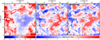 |
Fig. A.1. Example reconstruction of a 2D reionisation time map from a 2D map of the 21 cm signal taken at a redshift of z = 11. The left and middle panels are the brightness temperature and reionisation time fields generated by a 21cmFAST simulation. The right panel is the reconstruction of the reionisation times with the neural network designed to reproduce the true reionisation time map of the middle panel. Both treion(r) maps are dimensionless. |
We used a convolutional neural network (CNN) algorithm that can learn and detect complex patterns within images. In particular, we developed a U-net that takes an image as input and reconstructs another image as output: in our case, the inputs are 2D 21 cm maps at a given redshift (such as the one in the left panel of Fig. A.1) and the CNN will learn to construct outputs that will be as close as possible to the corresponding 2D reionisation time maps (such as the one in the middle panel of Fig. A.1). We therefore constructed data sets of 50 21cmFAST simulations that have a size of 256 cMpc/h with a resolution of 1 cMpc/h, from which we extract 128 × 128 images. These images are split into a training set on which the CNN will learn to reconstruct treion(r) and a validation set to check its performance. In that paper, we do not smooth the reionisation time maps.
With this U-net, we are able to reconstruct reionisation time maps from observation-like maps with levels of correspondence to the true maps that vary with the observational redshift. For z ∈ [8 − 12], 65% to 96% of treion(r) signal is well reconstructed. The reconstructed map shown in the right panel of Fig. A.1 was obtained with 21 cm maps taken at z = 11, which is one of the redshifts that returns the best results. We can see that in the process, and even for the best reconstructions, the small scales are smoothed out of the predicted treion(r) maps compared to the true ones, which is to be improved in future works. In Hiegel et al. (in preparation), we quantify the performance of the CNN via many diagnostics and show for example that we can extract an ionisation history that is consistent with the ones from the 21cmFAST simulations. This means that we can extract information about the evolution of the reionisation process and its topology simply from a 21 cm map obtained at a single redshift.
Appendix B: Calculation of the moment of a field and its derivatives from a given power spectrum
In this work, we use the spectral moments σi (for i ∈ ℕ) of the field of interest in order to normalise our fields, or because they appear in spectral parameters (defined in Eq. 6). These moments are only defined by the power spectrum of the field. The zeroth-order moment of a field is simply the standard deviation of the field, the first-order moment is the standard deviation of the first derivative of the field, and so on, as written in Eq. 2.
The moments can be expressed as follows (Bardeen et al. 1986; Pogosyan et al. 2009b; Gay 2011):
 (B.1)
(B.1)
where i ∈ ℕ corresponds to the number of derivation of the field, and d is the dimension of the field (in our case, d = 2). In our case, we are interested in the power spectra of the reionisation field, which are defined in Eq. 9, and which have two slopes in logarithmic scales (in his thesis, Gay (2011) presented the calculation for a power spectrum with one slope in logarithmic scales). To do so, we need the gamma functions, defined below:
 (B.2)
(B.2)
The integral within the moments can then be separated into two integrals where the cut is at the threshold kthresh separating the two parts of the power spectrum:
![Mathematical equation: $$ \begin{aligned} \begin{aligned} \sigma _i^2&= \frac{ 2\pi ^{\frac{d}{2}} }{ \Gamma \left(\frac{d}{2}\right) } \Biggl [ \int _0^{k_{\mathrm{thresh}}} k^{2i} \mathcal{P} _k k^{d-1} dk + \int _{k_{\mathrm{thresh}}}^\infty k^{2i} \mathcal{P} _k k^{d-1} dk \Biggr ] \\&= \frac{ A_2 2\pi ^{\frac{d}{2}} }{ \Gamma \left(\frac{d}{2}\right) } \Biggl [ \frac{A_1}{A_2} \int _0^{k_{\mathrm{thresh}}} k^{d-1+2i+n_1} e^{-2R_f^2k^2} dk \\&\qquad \qquad + \int _{k_{\mathrm{thresh}}}^\infty k^{d-1+2i+n_1} e^{-2R_f^2k^2} dk \Biggr ] \\&= \frac{ A_2 2\pi ^{\frac{d}{2}} }{ \Gamma \left(\frac{d}{2}\right) } \Biggl [ \frac{A_1}{A_2} \left(\frac{1}{\sqrt{2}R_f}\right)^{d+2i+n1} \int _0^{2R_f^2k_{\mathrm{thresh}}^2} k^{\frac{d+n_1}{2}-1} e^k dk \\&\qquad \qquad + \left(\frac{1}{\sqrt{2}R_f}\right)^{d+2i+n2} \int _{2R_f^2k_{\mathrm{thresh}}^2}^\infty k^{\frac{d+n_2}{2}-1} e^k dk \Biggr ]. \\ \end{aligned} \end{aligned} $$](/articles/aa/full_html/2023/04/aa44977-22/aa44977-22-eq44.gif) (B.3)
(B.3)
Now using the gamma functions defined above, we have the following expression for the spectral moments:
![Mathematical equation: $$ \begin{aligned} \begin{aligned} \sigma _i^2 = \frac{ A_2 2\pi ^{\frac{d}{2}} }{ \Gamma \left(\frac{d}{2}\right) }&\Biggl [ \frac{A_1}{A_2} \left(\frac{1}{\sqrt{2}R_f}\right)^{d+2i+n1} \gamma \Biggl (\frac{d+n1}{2}+i, 2R_f^2k_{\mathrm{thresh}}^2\Biggr ) \\&+ \left(\frac{1}{\sqrt{2}R_f}\right)^{d+2i+n2} \Gamma \Biggl (\frac{d+n2}{2}+i, 2R_f^2k_{\mathrm{thresh}}^2\Biggr ) \Biggr ]. \end{aligned} \end{aligned} $$](/articles/aa/full_html/2023/04/aa44977-22/aa44977-22-eq45.gif) (B.4)
(B.4)
The moments  have the same units as the power spectrum, but it is worth mentioning that the spectral parameters R0, R*, and γ remain dimensionless. We also note that they are only dependent on the dimension and the power spectrum parameters:
  .
.
Appendix C: Calculation of the PDF of the gradient norm of a field
Our fields of interest being Gaussian, we reiterate that their PDF can be written as follows:
 (C.1)
(C.1)
where x is a n-D vector function of the position and C = ⟨x ⊗ x⟩ is the covariance matrix. To compute a PDF depending on the field and its first derivative, we use  .
.
The covariance matrix of a 2D field F is the following:
 (C.2)
(C.2)
Using the normalised variables x, x1, and x2, the covariance matrix becomes:
 (C.3)
(C.3)
All the components of the PDF are now known, and after calculations, it is expressed as follows (and Eq. 15 is retrieved):
 (C.4)
(C.4)
As we are interested in PDFs that only depend on the first derivative of F, an integration on the field values x is done (thanks to the Gaussian integral  ):
):
 (C.5)
(C.5)
Moreover, we are interested in the norm of the gradient of the field, which is why we make a change of variable and introduce  . This is, more precisely, a change of variables in 2D polar coordinates:
![Mathematical equation: $$ \begin{aligned} \forall \theta \in [0,2\pi ], \quad {\left\{ \begin{array}{ll} x_1 = w\cos (\theta ), \\ x_2 = w\sin (\theta ). \\ \end{array}\right.} \end{aligned} $$](/articles/aa/full_html/2023/04/aa44977-22/aa44977-22-eq56.gif) (C.6)
(C.6)
With this change of variable, and as the PDF is independent of the introduced angle θ, we can write:
 (C.7)
(C.7)
with a rewritten PDF depending only on the norm of the gradient of the field:
 (C.8)
(C.8)
Appendix D: Reionisation redshift field analyses
The reionisation time and redshift fields are related to the same expression linking time and redshift:
 (D.1)
(D.1)
with a the scale factor. With this definition, they have opposite monotonies, which has consequences for a topological study. Indeed, there are small differences between the two fields : treion(r) increases more rapidly as zreion(r) decreases, and this causes some distinction in gaussianity analyses.
The aim of this Appendix is only to present a few results for the reionisation redshift field (zreion(r)), which presents some differences from the reionisation time field. To remain brief, we focus on the EMMAzreion(r). From the same simulation described in Sect. 2.1, we can extract 100 slices of the reionisation redshift field that are also smoothed with a Gaussian kernel of standard deviation Rf ∈ {1, 2, 6}, and normalised as below:
 (D.2)
(D.2)
with  the mean of each field.
  is the expected standard deviation of the field. The average and standard deviation of the reionisation redshift fields are given in Table 1. The power spectrum of the reionisation redshift field is also fitted as described in Sect. 2.1, and the resulting parameters are shown in Table 3.
We again generate 100 GRFs with the proper power spectrum to compare zreion(r) to them; these GRFs are also smoothed and normalised as described in Sect. 2.4. The resulting predictions for the reionisation time field are also calculated for the reionisation redshift field and shown below. The expressions are slightly modified for zreion(r), changing some integral limits or signs.
From Eq. 11, we can calculate the fraction of ionised volume of the reionisation redshifts in the same way as we did for the reionisation times. Here, the number of values that have a redshift higher than the threshold is equivalent to the number of cells that have already reionised. This therefore corresponds directly to the fraction of ionised volume QHII, as written below:
 (D.3)
(D.3)
As in the previous section, the filling factor of the gradient norm of redshift fields can be obtained from the joint PDF of Eq. 15, and is defined as follows:
 (D.4)
(D.4)
As it is symmetric, the isocontour length is the same for the reionisation time and redshift fields, for which the expression is reiterated below:
 (D.5)
(D.5)
The maxima of the reionisation redshift slices and the GRFs can be extracted with DisPerSE, as explained is Sect. 3.4. Their distribution can be theoretically calculated the same way as for the minima (as described in Sect. 3.4.2). We obtain the following distribution, where only some signs have changed:
![Mathematical equation: $$ \begin{aligned} \begin{aligned} \frac{\partial n_{\mathrm{max}}}{\partial \nu }&= \frac{ \exp \left({\frac{-\nu ^2}{2}}\right) }{ \sqrt{2\pi }R_*^2 } \left[1 + \mathrm{erf}{ \left(\frac{\gamma \nu }{\sqrt{2(1-\gamma ^2}} \right) }\right] K_1(\nu ,\gamma ) \\&+ \frac{ \exp \left(\frac{-3\nu ^2}{6-4\gamma ^2}\right) }{ \sqrt{2\pi (1-\frac{2}{3}\gamma ^2)}R_*^2 } \left[1 + \mathrm{erf}{ \left(\frac{\gamma \nu }{\sqrt{2(1-\gamma ^2)(3-2\gamma ^2)}} \right)} \right] K_2 \\&+ \frac{ \exp \left(\frac{-\nu ^2}{2(1-\gamma ^2)}\right) }{ \sqrt{2\pi (1-\gamma ^2)}R_*^2 } \left[1 + \exp \left( \frac{\nu ^2}{2(1-\gamma ^2)} \right) \right] K_3(\nu ,\gamma ). \\ \end{aligned} \end{aligned} $$](/articles/aa/full_html/2023/04/aa44977-22/aa44977-22-eq66.gif) (D.6)
(D.6)
As the reionisation redshift field has an opposite monotony compared to the reionisation time field, the skeleton of treion(r) is equivalent to the anti-skeleton of zreion(r). The anti-skeleton joins minima together passing through saddle points, and can also be extracted from the fields thanks to DisPerSE. The distribution of the anti-skeleton lengths are calculated in the same way as the skeleton-length distribution. Gay et al. (2012) informs us that this results in the same expression as that for the skeleton length (see Eq. 27) but with ν that becomes −ν, as follows:
![Mathematical equation: $$ \begin{aligned} \begin{aligned} \frac{\partial L^\mathrm{skel}}{\partial \nu }&= \frac{1}{\sqrt{2\pi } R_*} \exp ^{-\frac{\nu ^2}{2}} \Biggr [ \frac{1}{8\sqrt{\pi }} (\sqrt{\pi } - 2 \gamma \nu ) \left( 1 + \mathrm{erf}\left( \frac{- \gamma \nu }{\sqrt{2(1-\gamma ^2)}} \right) \right) \\&+ \frac{\sqrt{1-\gamma ^2}}{2\sqrt{2}\pi } \exp \left( - \frac{\gamma ^2\nu ^2}{2(1-\gamma ^2} \right) \Biggr ]. \\ \end{aligned} \end{aligned} $$](/articles/aa/full_html/2023/04/aa44977-22/aa44977-22-eq67.gif) (D.7)
(D.7)
In this short result section, we only show figures that highlight the discrepancies between the reionisation time and redshift fields. We begin with the 2D histograms of the gradient norm of zreion(r) versus zreion(r) for the EMMA simulation in Fig. D.1. On the first row, there are the cosmological fields, and on the second row, there are the GRFs. There is again a ‘symmetrisation’ when the size of the Gaussian kernel increases (i.e. Rf increases), although it is less pronounced than for the reionisation time field (see Fig. 9). On Fig. D.2, we show the maxima PDF of the EMMA reionisation redshift fields (with the crosses) of the corresponding GRFs (with the dashed lines), and the prediction (in black). Comparing these to the minima PDF of the EMMA reionisation time field (see Fig. 13), we can see that the treion(r) minima PDFs are closer to the GRF ones than the zreion(r) maxima PDFs, which again shows that treion(r) is more Gaussian than zreion(r). With these PDFs, we can again see the effect of the non-linear relation between zreion(r) and treion(r), which affects the x-axis. Indeed, for the smallest smoothing, the difference between the time and redshift of reionisation is evident: zreion(r) underestimates the number of critical points (that are reionisation seeds) with respect to treion(r). These figures globally show that the reionisation time field is more Gaussian than the reionisation redshift field, which is due to the non-linear relation between time and redshift, and which affects all the statistics studied in this paper.
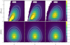 |
Fig. D.1. Two-dimensional PDFs of the gradient norms with respect to the values of the fields of every run for each field and different smoothings (Rf ∈ {1, 2, 6}, see each column). The first row corresponds to the EMMA reionisation redshifts, and the second row to their corresponding GRFs. The grey-scale lines are the isocontours of the histograms. Here, ν represents the value of the normalised reionisation redshifts. |
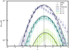 |
Fig. D.2. Distribution of the critical points of the fields for the different smoothings (in colours). The median of every run is computed for each field. The dashed lines correspond to the GRFs, and the crosses are for the EMMA reionisation redshift fields. The black lines are the theoretical predictions. The shaded areas and the error bars represent the dispersion around the median (1st and 99th percentiles) of the GRFs and treion(r), respectively. The black dotted vertical lines represent the average of the predictions. Here, ν represents the value of the normalised reionisation redshifts. |
All Tables
Average and standard deviation of both EMMA and 21cmFAST reionisation time and redshift fields.
Angular resolutions corresponding to the size of the smoothing kernel applied to our simulation at a redshift z = 6.905.
Parameters defining the power spectra of the reionisation time and redshift fields (treion(r) and zreion(r)) for both EMMA and 21cmFAST simulations.
All Figures
|
Fig. 1. Schematic summarising the use of the reionisation time field (on the right): it allows us to use only one field instead of a series of many snapshots of binary ionised fraction (on the left) for example. |
| In the text | |
|
Fig. 2. Two-dimensional slices related to the EMMA reionisation time field that are smoothed with a Gaussian kernel with a standard deviation of Rf = 6. The top left panel shows treion(r) with its minima (black stars). The top right panel shows treion(r) with its skeleton (black lines). The bottom left panel shows the isocontours of treion(r), with its minima again in black stars. Here, the reionisation time field is normalised to put its mean at a value of 0, and its standard deviation at 1. The bottom right panel shows the norm of the gradient of treion(r). |
| In the text | |
|
Fig. 3. Two-dimensional slices of the EMMA reionisation time field (first row) and the 2D GRFs obtained with the corresponding power spectrum (second row). Each column corresponds to different smoothings, with from left to right, Rf ∈ {1, 2, 6}. All the fields are normalised. |
| In the text | |
|
Fig. 4. Fitting (in dashed lines) of the reionisation time power spectra. The straight lines correspond to the power spectrum measured on the fields of each simulation (EMMA in blue and 21cmFAST in brown). The fittings are done on the average logarithmic power spectrum of every 2D slice for each field. The fields are not normalised when the fitting is carried out. |
| In the text | |
|
Fig. 5. Power spectra of the GRFs (coloured dotted lines) and EMMA reionisation times (coloured crosses). All 100 runs have been averaged to show a mean power spectrum for each set of simulations. The theoretical power spectra are shown both with and without an incorporated smoothing by the dashed and straight red lines, respectively. Three different smoothings are represented with Rf ∈ {1, 2, 6}. |
| In the text | |
|
Fig. 6. Fraction of ionised volume for the different smoothings (in colours). The median of every run is computed for each field. The dashed lines correspond to the GRFs, and the crosses are for the EMMA reionisation time field. The black lines are the theoretical predictions. The shaded areas and the error bars represent the dispersion around the median (1st and 99th percentiles) of the GRFs and treion(r), respectively. Here, ν represents the value of the normalised reionisation times. |
| In the text | |
|
Fig. 7. Probability distribution function of the median of every run of the fields for the different smoothings (in colours). The dashed lines correspond to the GRFs, and the crosses are for the EMMA fields. The black lines are the theoretical predictions. The shaded areas and the error bars represent the dispersion around the median (1st and 99th percentiles) of the GRFs and treion(r), respectively. Here, ν represents the value of the normalised reionisation times. |
| In the text | |
|
Fig. 8. Two-dimensional slices of the norm of the EMMA reionisation time gradient (first row) and the norm of the GRF gradient obtained with the corresponding power spectrum (second row). Each column corresponds to different smoothings, with from left to right, Rf ∈ {1, 2, 6}. |
| In the text | |
|
Fig. 9. Two-dimensional PDFs of the gradient norms with respect to the values of the fields of every run for each field and different smoothings (Rf ∈ {1, 2, 6}, see each column). The first row shows the EMMA reionisation times, and the second row their corresponding GRFs. The grey-scale lines are the isocontours of the histograms. Here, ν represents the value of the normalised reionisation times. |
| In the text | |
|
Fig. 10. Filling factors of the gradient norms of the fields for the different smoothings (in colours). The median of every run is computed for each field. The dashed lines correspond to the GRFs, and the crosses are for the EMMA reionisation time fields. The black lines are the theoretical predictions. The shaded areas and the error bars represent the dispersion around the median (1st and 99th percentiles) of the GRFs and treion(r), respectively. Here, w represents the value of the gradient norm of the reionisation times. |
| In the text | |
|
Fig. 11. Isocontours of 2D slices of the EMMA reionisation time field (first row) and of the 2D GRF obtained with the corresponding power spectrum (second row). Each column corresponds to a different smoothing, with Rf ∈ {1, 2, 6} from left to right. All fields are normalised. Eight levels of contours are represented with the colours. |
| In the text | |
|
Fig. 12. Distribution of the isocontour length for the different smoothings (in colours). The median of every run is computed for each field. The dashed lines correspond to the GRFs, and the crosses show the EMMA reionisation time field. The black lines are the theoretical predictions. The shaded areas and the error bars represent the dispersion around the median (1st and 99th percentiles) of the GRFs and treion(r), respectively. Here, ν represents the value of the normalised reionisation times. |
| In the text | |
|
Fig. 13. Distribution of the critical points of the fields for the different smoothings (in colours). The median of every run is computed for each field. The dashed lines correspond to the GRFs, and the crosses are for the EMMA reionisation time fields. The black lines are the theoretical predictions. The shaded areas and the error bars represent the dispersion around the median (1st and 99th percentiles) of the GRFs and treion(r), respectively. The black dotted vertical lines represent the average of the predictions. Here, ν represents the value of the normalised reionisation times. |
| In the text | |
|
Fig. 14. Distribution of the skeleton length of the fields for the different smoothings (in colours). The median of every run is computed for each field. The dashed lines correspond to the GRFs, and the crosses are for the EMMA reionisation time fields. The black lines are the theoretical predictions. The shaded areas and the error bars represent the dispersion around the median (1st and 99th percentiles) of the GRFs and treion(r), respectively. The black dotted vertical lines represent the average of the predictions. Here, ν represents the value of the normalised reionisation times. |
| In the text | |
|
Fig. 15. Two-dimensional PDFs of the gradient norms with respect to the values of the fields of every run for each field and different smoothings (Rf ∈ {1, 2, 6}, see each column). The first row corresponds to the 21cmFAST reionisation times, and the second row to their corresponding GRFs. The grey-scale lines are the isocontours of the histograms. Here, ν represents the value of the normalised reionisation times. |
| In the text | |
|
Fig. 16. Fraction of ionised volume of the fields for the different smoothings (in colours). The median of every run is computed for each field. The dashed lines correspond to the GRFs, and the crosses are for the 21cmFAST reionisation time fields. The black lines are the theoretical predictions. The shaded areas and the error bars represent the dispersion around the median (1st and 99th percentiles) of the GRFs and treion(r), respectively. Here, ν represents the value of the normalised reionisation times. |
| In the text | |
|
Fig. 17. Distribution of the skeleton length of the fields for the different smoothings (in colours). The median of every run is computed for each field. The dashed lines correspond to the GRFs, and the crosses are for the 21cmFAST reionisation time fields. The black lines are the theoretical predictions. The shaded areas and the error bars represent the dispersion around the median (1st and 99th percentiles) of the GRFs and treion(r), respectively. The black dotted vertical lines represent the average of the predictions. Here, ν represents the value of the normalised reionisation times. |
| In the text | |
|
Fig. A.1. Example reconstruction of a 2D reionisation time map from a 2D map of the 21 cm signal taken at a redshift of z = 11. The left and middle panels are the brightness temperature and reionisation time fields generated by a 21cmFAST simulation. The right panel is the reconstruction of the reionisation times with the neural network designed to reproduce the true reionisation time map of the middle panel. Both treion(r) maps are dimensionless. |
| In the text | |
|
Fig. D.1. Two-dimensional PDFs of the gradient norms with respect to the values of the fields of every run for each field and different smoothings (Rf ∈ {1, 2, 6}, see each column). The first row corresponds to the EMMA reionisation redshifts, and the second row to their corresponding GRFs. The grey-scale lines are the isocontours of the histograms. Here, ν represents the value of the normalised reionisation redshifts. |
| In the text | |
|
Fig. D.2. Distribution of the critical points of the fields for the different smoothings (in colours). The median of every run is computed for each field. The dashed lines correspond to the GRFs, and the crosses are for the EMMA reionisation redshift fields. The black lines are the theoretical predictions. The shaded areas and the error bars represent the dispersion around the median (1st and 99th percentiles) of the GRFs and treion(r), respectively. The black dotted vertical lines represent the average of the predictions. Here, ν represents the value of the normalised reionisation redshifts. |
| In the text | |
Current usage metrics show cumulative count of Article Views (full-text article views including HTML views, PDF and ePub downloads, according to the available data) and Abstracts Views on Vision4Press platform.
Data correspond to usage on the plateform after 2015. The current usage metrics is available 48-96 hours after online publication and is updated daily on week days.
Initial download of the metrics may take a while.