| Issue |
A&A
Volume 653, September 2021
|
|
|---|---|---|
| Article Number | A58 | |
| Number of page(s) | 14 | |
| Section | Cosmology (including clusters of galaxies) | |
| DOI | https://doi.org/10.1051/0004-6361/202140515 | |
| Published online | 08 September 2021 | |
Using the sample variance of 21 cm maps as a tracer of the ionisation topology
1
Université Paris-Saclay, CNRS, Institut d’Astrophysique Spatiale, 91405 Orsay, France
2
Department of Physics, Blackett Laboratory, Imperial College, London SW7 2AZ, UK
3
Department of Physics and McGill Space Institute, McGill University, Montreal H3A 2T8, QC, Canada
e-mail: This email address is being protected from spambots. You need JavaScript enabled to view it.
4
Kapteyn Astronomical Institute, University of Groningen, PO Box 800, 9700 AV Groningen, The Netherlands
Received:
8
February
2021
Accepted:
28
June
2021
Abstract
Intensity mapping of the 21 cm signal of neutral hydrogen will yield exciting insights into the Epoch of Reionisation and the nature of the first galaxies. However, the large amount of data that will be generated by the next generation of radio telescopes, such as the Square Kilometre Array, as well as the numerous observational obstacles to overcome, require analysis techniques tuned to extract the reionisation history and morphology. In this context, we introduce a one-point statistic, which we refer to as the local variance, σloc, that describes the distribution of the mean differential 21 cm brightness temperatures measured in two-dimensional maps along the frequency direction of a light cone. The local variance takes advantage of what is usually considered an observational bias, the sample variance. We find the redshift-evolution of the local variance to not only probe the reionisation history of the observed patches of the sky, but also trace the ionisation morphology. This estimator provides a promising tool to constrain the midpoint of reionisation as well as gain insight into the ionising properties of early galaxies.
Key words: dark ages / reionization / first stars / methods: statistical
© A. Gorce et al. 2021
 Open Access article, published by EDP Sciences, under the terms of the Creative Commons Attribution License (https://creativecommons.org/licenses/by/4.0), which permits unrestricted use, distribution, and reproduction in any medium, provided the original work is properly cited.
1. Introduction
The Epoch of Reionisation (EoR) represents an essential time within the first billion years of the Universe, when the first light sources formed and gradually ionised the neutral hydrogen gas in the intergalactic medium (IGM). However, the exact properties of these first light sources remain uncertain. With the help of the Cosmic Microwave Background (CMB) small- and large-scale data (Planck Collaboration Int. XLVII 2016), observations of the luminosity functions of star-forming galaxies (Bouwens et al. 2015), and H I absorption troughs in the spectra of quasars (McGreer et al. 2015; Bañados et al. 2018), we have obtained constraints on the ionisation history, that is the time evolution of the ionisation fraction of the hydrogen gas in the IGM (Robertson et al. 2015; Gorce et al. 2018). However, reionisation is patchy, with different regions of the sky being ionised at different times.
For this reason, the observation of the time evolution of the 21 cm brightness temperature maps at redshifts z ≥ 5, tracing the neutral hydrogen gas in the IGM and referred to as 21 cm tomography is highly anticipated and should be achieved with the next generation of radio interferometers, such as the Square Kilometre Array (SKA, Koopmans et al. 2015) or the Hydrogen Epoch of Reionization Array (HERA, DeBoer et al. 2017). Such maps will allow us to trace the reionisation process, in particular the time and spatial evolution of the ionised regions around the first light sources. Constraints from current observations imply that star-forming galaxies were the main drivers of reionisation. The topology of the ionised regions provides a tracer of the physical properties of these galaxies and their distribution in the IGM (Zahn et al. 2007; McQuinn et al. 2007; Mesinger et al. 2011). In the recent years, many statistical tools of various levels of complexity have been developed to extract information about the ionisation sources from these maps, but this is complicated by the cosmological signal often being swamped with thermal noise and foregrounds (Chapman & Jelić 2019; Liu & Shaw 2020; Hothi et al. 2021; Gagnon-Hartman et al. 2021). While the power spectrum of the 21 cm signal has been the main tool to extract the Gaussian part of the 21 cm signal from reionisation (e.g., Greig et al. 2021; Pagano & Liu 2020), three-point statistics have been increasingly studied to access the non-Gaussian part of the signal (Shimabukuro et al. 2016; Majumdar et al. 2018; Gorce & Pritchard 2019; Watkinson et al. 2019; Hutter et al. 2020).
Choosing a simpler approach, many works have focussed on the one-point probability distribution function (PDF) of the differential 21 cm brightness temperature δTb and its moments (Ciardi & Madau 2003; Furlanetto et al. 2004; Mellema et al. 2006). Since the morphology of this 21 cm signal is driven by the morphology of the ionised regions during the EoR, it is informative to assess the PDF of the ionisation fraction distribution. For example, for a binary ionisation field, where pixels are either fully ionised or fully neutral, the corresponding one-point PDF can be derived as a combination of Dirac delta functions δ:
 (1)
(1)
where  is the filling fraction – or the mean ionisation level of the simulation. From this PDF, analytic expression for statistical moments can be derived. Comparing how these statistical moments, derived numerically from more sophisticated models and simulations, deviate from these analytical expressions provide us with hints on the nature of reionisation (Gluscevic & Barkana 2010), such as its reionisation topology (e.g., inside-out or outside-in, see Watkinson & Pritchard 2014) and its global reionisation history (Bittner & Loeb 2011; Patil et al. 2014), even when derived from dirty 21 cm signal images or after foreground removal (Harker et al. 2009). Kittiwisit et al. (2018) show that HERA will be able to detect the variance of the 21 cm brightness temperature field from reionisation with high sensitivity, by averaging over measurements from multiple fields. However, these one-point statistics lack information on the correlations between pixels. For this reason, Barkana & Loeb (2008) have extended this formalism by analysing the one-point PDF of the difference in the differential 21 cm brightness temperature measured at two points.
In this work, we present a new higher-order one-point statistic, to which we refer to as the local variance σloc. This local variance can be computed by dividing the total volume of a three-dimensional field x(r) into N sub-volumes {Vα}1 ≤ α ≤ N. Let us consider a sub-volume Vα centred on rα, described by the window function
 (2)
(2)
where Lj is the length of each of the three sides of the sub-volume. Then the local variance is defined by:
![Mathematical equation: $$ \begin{aligned} {{\sigma _{\rm loc}}}^2 \equiv \sum _{\alpha =1}^N \left[ \int \mathrm{d}^3\boldsymbol{r}\ W_\alpha (\boldsymbol{r-r}_\alpha )\, x(\boldsymbol{r}) \right]^2 - \bar{x}^2, \end{aligned} $$](/articles/aa/full_html/2021/09/aa40515-21/aa40515-21-eq4.gif) (3)
(3)
with  being the expectation value of the field. In other words, it is the variance of the distribution of the means of the sub-volumes. In this work, we mostly focus on the case where the sub-volumes considered are slices cut through the cube. It is clear from this definition that this estimator is based on sample variance and will be zero for a sufficiently large data cube. However, for smaller fields, it will provide us with information about the morphology imprinted in the field x(r), as it – contrary to usual one-point statistics, encompasses information on the correlations between pixels. It is interesting to note that previous works have also considered estimators computed in sub-volumes of data: for example, Chiang et al. (2015), Giri et al. (2019) investigate the power spectrum of sub-volumes, also referred to as the position-dependent power spectrum. However, in contrast to these approaches, our estimator will benefit from its simplicity.
We fully introduce the local variance and give its phenomenological definition in Sect. 3. In Sect. 4, we apply this statistic to a range of simulations, that we describe in Sect. 2, and find that its evolution with redshift is a good tracer of the ionisation history and topology, even when including observational effects, such as thermal noise and telescope resolution. We conclude in Sect. 5. In the following, all distances are in comoving units and the cosmology used is the best-fit cosmology derived from Planck 2015 CMB data (Planck Collaboration I 2016): h = 0.6774, Ωm = 0.309, Ωbh2 = 0.02230, Yp = 0.2453, σ8 = 0.8164 and TCMB = 2.7255 K. We use interchangeably the terms filling fraction and ionisation level to describe the mean of ionisation fields  .
.
2. Simulations
We applied our analysis to two types of simulations in order to check that our results are robust against different ways of modelling reionisation. First, we consider the rsage simulations (Seiler et al. 2019), which are based on a N-body simulation with 24003 dark matter (DM) particles and a side length of 160 Mpc. A modified version of the Semi-Analytic Galaxy Evolution (SAGE) model (Croton et al. 2016), which accounts for delayed supernovae feedback and radiative feedback, describes the evolution of the galaxies and their properties within the simulation. The ultraviolet background (UVB) is generated with the semi-numerical code cifog (Hutter 2018a,b). cifog also follows the time and spatial evolution of the ionised hydrogen regions in the simulation box. Three different prescriptions for the escape fraction of ionising photons from galaxies into the IGM, fesc, cover the physical plausible parameter space: In rsage const, fesc is considered to be constant regardless the redshift and properties of the galaxies. Its value is fixed to 20% (Robertson et al. 2015). In rsage fej, fesc scales with the fraction of gas ejected from each galaxy, fej. In rsage SFR, fesc scales with the star formation rate of each galaxy, resulting in fesc effectively scaling with halo mass. These different ionising properties result in a different morphology of the ionisation fields, with rsage SFR exhibiting the largest ionised bubbles at a given global ionisation fraction  . This is illustrated in the upper panels of Fig. 1, which show the binary ionisation fields of the three simulations at
  , when the simulations are 30% ionised. Since the three rsage simulations have the same underlying DM distribution and have been tuned to reproduce the Planck optical depth, we find their ionisation histories to be very similar (see the upper right panel of Fig. 4). However, due to the different descriptions of fesc, they diverge slightly towards the end of the reionisation process, with rsage SFR reaching a fully ionised IGM by Δz ≃ 0.1 earlier than rsage fej.
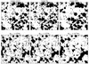 |
Fig. 1. Binary ionisation fields cut through the three rsage simulations (upper panels) and the three 21cmFAST runs (lower panels) described in Sect. 2 at |

Secondly, we use the publicly available 21cmFAST simulation (Mesinger & Furlanetto 2007; Mesinger et al. 2011)1. 21cmFAST is a semi-numerical code using excursion-set formalism (Furlanetto et al. 2004): starting from a matter overdensity field, it assumes each cell to be ionised when the number of photons exceeds the number of baryons in the respective cell. 21cmFAST has multiple simulation parameters that can be varied to change the underlying physical model, which again can result in different reionisation histories and morphology. Here, we choose to vary the parameter Mturn, the turnover mass, which corresponds to the minimum halo mass below which star formation is suppressed exponentially. During the EoR, Mturn = 108 M⊙ would correspond roughly to a virial temperature of 104 K. We generate three simulations, with the same dimensions and resolution as the rsage simulations, and assume Mturn = 108 M⊙, 109 M⊙ and 1010 M⊙, to which we refer as M8, M9 and M10 in the following, respectively. Their global ionisation histories can be seen in the lower-right panel of Fig. 4. The higher number of sources in M8 leads to an earlier reionisation of the IGM than in the other two simulations. In M10, however, reionisation is delayed until haloes of sufficient mass have formed. Since more massive sources are also more efficient at ionising their surroundings, M10 has on average larger ionised regions than M8 and M9. This can be seen in the lower panels of Fig. 1, which show the snapshots of the ionisation fields of M8, M9 and M10 at  .
.
Extracting the ionisation fields from the differential 21 cm brightness temperature maps remains difficult (e.g., Malloy & Lidz 2013; Beardsley et al. 2015; Datta et al. 2016; Giri et al. 2018; Mangena et al. 2020) due to their contamination by instrumental effects and foregrounds (Gluscevic & Barkana 2010; Chapman et al. 2013; Liu & Shaw 2020): hence, we need statistical tools that we can apply directly to these 21 cm maps. For this reason we apply our new one-point statistics also to the differential 21 cm brightness temperature δTb cubes in the following. From the rsage neutral fraction, xH I = 1 − xe, and baryon density, δb, cubes, we construct the corresponding δTb fields following Pritchard & Loeb (2012):
 (4)
(4)
Here, we assume that X-rays have heated the gas sufficiently such that the spin temperature of the neutral hydrogen gas exceeds the CMB temperature considerably. Because this work is a proof-of-concept for the local variance, we choose to limit our analysis to results using this assumption. However, recent works have shown that the CMB temperature might actually not be negligible during reionisation (Heneka & Mesinger 2020). For the 21cmFAST simulations, the brightness temperature cubes are computed directly by the simulation package, which allows a more complete derivation than the approximation given in Eq. (4), namely including velocity corrections. Since interferometric observations will only measure the fluctuations in the 21 cm signal, we subtract each cube by its mean so that the 21 cm cubes have a mean zero. In practice, an interferometer measures a mean-zero map for each frequency bin, which is equivalent to saying that each slice of this cube has a mean zero and would make the local variance vanish. Hence, we assume that using N slices of a coeval cube at fixed redshift z is equivalent to considering N small patches of a larger field-of-view at fixed frequency. We leave a detailed investigation of this hypothesis for future work.
3. Methods
In order to build intuition for this new estimator, we first look at the ionisation fields of our simulations. We obtain the 3D variance of the ionisation field of a coeval cube extracted from the simulations, at a given redshift z and global ionisation level  , by computing:
 (5)
(5)
where the ionisation level of a cell (i, j, k) can be either xi, j, k(z) = 0 or 1. It is possible to relate the variance  of a 3D field xe(r) to its 2-point correlation function (2-PCF) ξ2 and, in turn, to its power spectrum P(k)2. With this relation, we can estimate the variance of the EoR 21 cm signal by measuring its power spectrum. In this context, Patil et al. (2014) has used forecast LOFAR observations and the inferred redshift-evolution of σwhole to constrain the midpoint and duration of reionisation. From a topological point of view, examining the evolution of σwhole with
  allowed Watkinson & Pritchard (2014) to differentiate between outside-in and inside-out scenarios of reionisation. However, in all the simulations analysed in this work, reionisation proceeds inside-out. As such, we find for our three rsage simulations only a ∼1% deviation from the theoretical parabola which can be derived from the PDF of ionised pixels P(xe) given in Eq. (1):
 (8)
(8)
The results also hold for the 21cmFAST simulations and higher order cumulants, such as the skewness and the kurtosis. Therefore, the distribution of pixels throughout the whole box cannot differentiate between the simulations, as it mainly traces the reionisation history. In particular, it does not account for the correlations between pixels, and hence cannot track morphological differences.
For this reason, we introduce the local variance, which is sensitive to the ionisation topology as it includes the small and large-scale correlations between points:
 (9)
(9)
Here, μ(k, z) is the mean value of the kth slice along the redshift direction3. We explain the derivation of this statistic by considering the three-dimensional binary ionisation field of the rsage const simulation. The ionisation field is a cube with N = 256 cells on a side, each cell having a width of Δx = 0.625 Mpc. Snapshots every 10 Myrs, tracking the reionisation process, are available. For each snapshot, we compute the average value μ of each of the N slices, each having a width of one cell along a chosen direction. Here, we assume this direction to be the redshift – or frequency – direction. The resulting distribution of N filling fractions {μ}0 ≤ k < N is centred around the filling fraction of the whole 3D box at the respective redshift,  . The left panel of Fig. 2 shows these distributions for redshifts 6 ≤ z ≤ 15. At the beginning of reionisation, the distribution is very narrow but widens as reionisation progresses and ionised bubbles grow, tracing the underlying clustered galaxy population and the increasing correlation between pixels. At the end of reionisation, the distribution is again very narrow as most pixels are fully ionised. In the right panel of the figure, we summarise our results by plotting the evolution of the standard deviation of these distributions σloc as a function of the global ionisation level (blue solid line).
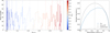 |
Fig. 2. Left panel: distribution of the ionisation levels of the N slices that can be carved out of the rsage const simulation along one direction. Each colour corresponds to one of 12 snapshots taken on the range 6.02 ≤ z ≤ 14.63, corresponding to different ionisation levels, represented as the solid vertical lines. Right panel: evolution of the standard deviations of each distribution with global reionisation history (blue solid line), compared to the standard deviation of the distribution of ionised pixels throughout the whole box (dashed line, divided by 10). |
As outlined in our motivation, we can see from Eqs. (5) and (9), that the local variance σloc describes the morphology of the considered field more accurately than the ordinary 3D variance σwhole, as it includes the variance of each slice. Indeed, if we consider Var(k) the variance of the k-th slice, then  , and it is easy to see that
 (10)
(10)
Furthermore, we note that since the 3D variance can be expressed in terms of the 2-PCF given in Eq. (7), the local variance is also given by
 (11)
(11)
where μ(r) is the mean of the slice located at r and Pμ(k) is the power spectrum of the 1D distribution of means {μ(r)}r ≤ L. Pμ(k) corresponds to the 3D power spectrum of the field, when only the modes along the frequency direction in Fourier space are kept and are rescaled by the area of the observational window in the sky plane: Pμ(k) = P(k)/L2 for k = (0, 0, kz). Selecting such modes can be done by using a specific window function, for example a Bessel function (Muñoz & Cyr-Racine 2021).
4. Results
4.1. Understanding the local variance
In this section, we analyse the evolution of the local variance of the rsage const simulation. In order to understand the impact of the ionisation fraction and density distributions on our estimator, we first discuss the local variance of the ionisation fraction fields before we analyse the local variance of the differential 21 cm brightness temperature maps. For clarity, we add a superscript to σloc, describing the field considered:  for the ionisation field,
  for the brightness temperature field.
We show the local variance of the ionisation field  of the rsage const simulation as a function of its mean in the right panel of Fig. 2. For comparison, we also plot the results for the scaled 3D variance, σwhole/10. The dotted vertical line indicates the midpoint of reionisation at
  , where σwhole is maximum (see Eq. (8)). On the other hand,
  (blue line) is slightly distorted compared to σwhole and reaches its maximum around
  . The location of the maximum indicates the moment when ionised and neutral regions are the largest, which will depend on the large-scale structure of the ionisation fields. We discuss this in more detail in the next Section when we compare different ionisation morphologies. To confirm the physical origin of this signal, we compute the local variance of a control test, consisting of a 3D box of the same resolution and size as our simulations, but randomly filled with ionised pixels to reach the considered ionisation level. Such a field will contain none of the correlations we aim at probing with the local variance and will actually be analogous to a box with white noise power spectrum. It can also be seen as a field made of many uncorrelated very small bubbles, which is close to the ionisation field at the very beginning of reionisation (see next paragraph). The resulting variance, close to zero and largely insignificant compared to what was obtained for the simulations, is shown as the black solid line in the right panel of Fig. 2.
In Fig. 3, we show the local variance of the δTb field of the rsage const simulation as a function of redshift (thick solid line) along with the local variances of the H I and δb fields and the covariance of the distributions of means for the ionisation field (xloc) and the 21 cm brightness temperate field (δb, loc). Because of correlations, the exact expression of  , given in Appendix A, does not equal the sum of the aforementioned three elements, but they are useful to understand the behaviour of
  . Overall, the redshift-evolution of the local variance
  traces the reionisation history and is similar to the one observed in Patil et al. (2014) for the 3D variance. At high redshift, before the onset of reionisation (z ≳ 12), the variance across slices comes from the underlying density field. As the first sources start ionising neutral hydrogen, zero pixels appear on the Gaussian δTb background (z ≃ 9 − 12), and homogenise the distribution (Gluscevic & Barkana 2010; Bittner & Loeb 2011), leading to a dip in the variance at z ≃ 9.5. At this point, the distribution of ionised regions is similar to the one of the control test, considered above, hence the small amplitude of the local variance. As reionisation proceeds, zero (ionised) pixels start tracing the reionisation morphology. As their number increases compared to the number of warm (neutral) pixels (which still follow a Gaussian distribution),
  starts mostly tracing the ionisation field and increases until reaching its maximum around the midpoint of reionisation, when both ionised and neutral regions are the largest. As more and more pixels are ionised, the global brightness temperature approaches zero and so does the local variance. A similar redshift evolution has been observed in the skewness of pixel distributions within two-dimensional brightness temperature maps (Harker et al. 2009) and can be recovered using a combination of analytical functions (Ichikawa et al. 2010; Patil et al. 2014). However, these theoretical functions do not say much about the time and spatial distribution of ionised regions.
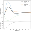 |
Fig. 3. Contributions to the local variance of the δTb field in the rsage const simulation (upper panel) and its reionisation history (lower panel). |
4.2. Comparing simulations
In order to understand how the ionisation morphology affects the characteristic features in σloc(z), which are the amplitude and ionisation fraction at which σloc(z) reaches its maximum, we compare  for all the simulations described in Sect. 2. Results for rsage and 21cmFAST are shown in the upper and lower panels of Fig. 4, respectively.
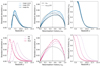 |
Fig. 4. Evolution of the standard deviation on the distribution of means measured in the set of N slices that can be carved out of the ionisation fields of simulations along one direction with redshift (left panel) and ionisation level (middle panel). Right panel: corresponding reionisation histories. Results for the three rsage simulations (upper panels) and the three 21cmFAST runs (lower panels) are compared. |
As we can see from the top right panel, the three rsage simulations show similar reionisation histories, and, therefore, the approximate locations of the minima and maxima of the local variance are similar. However, they differ in their amplitudes. Here, in contrast to what we have found for σwhole, there is a clear difference between the three rsage simulations: for example, at  , the local variances of rsage fej and rsage SFR are about 20% below and 20% above the one of rsage const, respectively. We find more variance between the rsage SFR slices, since the simulation exhibits larger ionised regions (Seiler et al. 2019). This can be understood as follows. Consider an ionisation field at a given global ionisation level
  . If the field is made of a few large ionised bubbles and we cut a slice through the box, we are more likely to pick up a large ionised region that will bias the filling fraction of the slice μ towards values larger than
  . Conversely, if the field is made of many small ionised regions, such as in the rsage fej simulation, the slices cut through the box are more likely to have similar μ values and
  will be lower.
We confirm these findings and extend our understanding of how the characteristics of  depend on the reionisation morphology by analysing the results we obtain for the three 21cmFAST simulations that differ in their reionisation history and morphology (see Fig. 1). When computing the local variance of the 21cmFAST ionisation fields, we find that, similarly to rsage, at a given ionisation level, the simulation with the on average largest ionised regions, M10, yields the largest
  values. This is in agreement with the findings of Gluscevic & Barkana (2010), who already noticed that if the ionising sources lie in more massive haloes in one simulation than another, the impact on the 3D pixel distribution is noticeable as the ionised regions are larger and more scarce at the same global ionisation fraction. Since the three 21cmFAST simulations exhibit not only different ionisation morphology but also different ionisation histories, the redshift-evolution of
  varies from one simulation to the other in addition to its variations in amplitude. This result implies that measuring the local variance of a field will help us to constrain the reionisation history.
Similar to the rsage simulations, the maximal local variance is also reached around the reionisation midpoint for the three 21cmFAST runs. In general, this is expected to happen when the derivative of the global signal with respect to redshift is maximal (Muñoz & Cyr-Racine 2021). During reionisation, we expect the signal to be maximal when both ionised and neutral regions are the largest. Applying the bubble size algorithm granulometry (Kakiichi et al. 2017) to the rsage simulations, we find this to be the case for all three simulations, at  (Hutter et al. 2020), which also corresponds to the measured maximum of the local variance in the simulations. Indeed, we find the maximum to be located at z = 8.4 ± 0.1, 6.7 ± 0.1 and 5.2 ± 0.1, corresponding to an ionisation level of
  , 0.65 ± 0.02 and 0.58 ± 0.02 for the M8, M9 and M10 simulations, respectively. Interestingly, this result holds when computing the local variance of a toy model, made of randomly located fully ionised bubbles. All the bubbles have the same initial radius and are grown by increasing the radius one pixel at a time until the whole box is ionised (details on this toy model can be found in Appendix B). In these toy models, the maximum local variance is always reached when the box is about 60% ionised, although slightly sooner when the initial bubble radius is larger. In Fig. 5, we show snapshots of the ionisation fields of the three 21cmFAST simulations at the redshift when they reach the maximum local variance. Interestingly, despite these snapshots corresponding to different ionisation levels and redshifts, they have their largest ionised regions in common. This indicates that, in contrast to its amplitude, the location of the maximum of the local variance is purely sensitive to the large-scale structure of the ionisation field. As the total number of ionising photons decreases in M8, M9 and M10, respectively, the large-scale ionised regions will reach their maximum size at lower redshifts; but due to the different ionising emissivity distributions across sources, the redshifts where the local variance becomes maximal will correspond to a different ionisation level of the box. For example, in Fig. 5, we see that the neutral regions are filled with many small ionised regions in M8, increasing the overall ionisation level of the simulation to a higher one than in M10 at the redshift of maximal local variance.
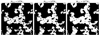 |
Fig. 5. Snapshots of the ionisation field at the maximum of the local variance for the M8, M9 and M10 simulations, corresponding to different redshifts and different ionisation levels: z = 8.4 and |


We have seen that differences in the ionisation morphology across simulations translate into differences in the amplitude of  , and differences in reionisation histories into translations in redshift. We now turn to the differential 21 cm brightness temperature fields which, as we have seen in the previous Section, encompass additional information from the ionisation morphology. Figure 6 shows the redshift-evolution of
  with redshift for the three rsage simulations (upper panel) and the three 21cmFAST runs (lower panel). We briefly note that the three rsage simulations show the same local variance at high redshifts (z ≳ 12), because
  is governed by the same underlying density field. However, as
  becomes sensitive to the ionisation field, its shape traces the reionisation history, while its amplitude is sensitive to the reionisation morphology: as observed for the ionisation field, here, the rsage SFR simulation, which has the largest ionised regions on average, exhibits the largest
  . However, this is not true for the 21cmFAST simulations: in contrast to what is expected, M10 exhibits the lowest amplitude in
  during reionisation. This is because M10 reionises later than M8, when the density field is more heterogeneous and the local variance of the density field larger; such that the anti-correlation between δb and xH I is stronger, adding negative signal to the local variance of the overall brightness temperature field (see Fig. 3). The pre-factor of Eq. (4), which is proportional to
  , also contributes to enhancing the signal at higher redshifts and hence to M8 showing a higher amplitude at its maximum because it is reached at a higher redshift. This also explains why M10 exhibits the shallowest dip at z ≃ 7 of the three simulations during cosmic dawn. Finally, the larger amplitudes of the local variance seen at high redshift (z ≳ 12 for M8, z ≳ 8 for M10) is found to be related to the extra terms included in the 21cmFAST derivation of the 21 cm brightness temperature compared to the simplified expression given in Eq. (4), namely the velocity field.
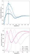 |
Fig. 6. Local variance of the 21 cm brightness temperature fields from the rsage (upper panel) and 21cmFAST (lower panel) simulation, as a function of redshift. Vertical dotted lines show the ionisation midpoint of the simulation of the corresponding colour. |
4.3. Observational effects
Many limitations related to the nature of instruments are expected to complicate the observation of the 21 cm signal from reionisation. For this reason, we consider the effects of thermal noise and angular resolution smoothing on our δTb maps and subsequent measurements of the local variance. In the following, we consider the performance characteristics of SKA1-Low (Braun et al. 2019), in an optimistic and a pessimistic case, corresponding respectively to a maximum baseline of bmax = 65 km and 2 km. In both cases, the total effective collecting area of Atot ∼ 105 m2 is frequency dependent. Indeed, the Australian interferometer will consist of about 2 × 10⁶ dipoles, gathered in 512 stations with 24 tiles per station. Each individual dipole will have an effective area of  , with λ21 being the redshifted 21 cm wavelength.
In order to apply the appropriate SKA1-Low angular smoothing to our δTb maps, we convolve each simulation cube (corresponding to a given redshift z) by a Gaussian kernel with a FWHM of θ(z) dc(z), with dc(z) being the comoving distance to redshift z and
 (12)
(12)
the angular resolution of the telescope. Because of the size of the SKA1-Low array, its angular resolution will be very high: It will range from 0.15 Mpc at z = 4 to 0.66 Mpc at z = 15, which is smaller than the resolution of our simulation grids (Δx = L/N = 0.625 Mpc) at all redshifts of interest. Consequently, the smoothed and original maps are very similar, and so will be the resulting σloc.
We then generate thermal random noise by drawing a noise value ni from a Gaussian distribution with a variance  for each pixel, with the variance given by (Watkinson & Pritchard 2014):
 (13)
(13)
Here, Δν is the frequency resolution of the experiment, which we match for computational efficiency to the resolution of the simulation Δx according to ![Mathematical equation: $ \Delta \nu =H_0 \nu_0 \sqrt{\Omega_{\mathrm{m}}} \Delta x /[c \sqrt{(1+z)}] $](/articles/aa/full_html/2021/09/aa40515-21/aa40515-21-eq56.gif) with H0 being the Hubble constant and ν0 the rest-frame 21 cm frequency. SKA1-Low is expected to have a much better frequency resolution than the comoving cell size of 0.625 Mpc used in this work, with a channel width of 5.4 kHz at a nominal frequency of 100 MHz (Braun et al. 2019). A thinner resolution will be beneficial to local variance analyses (see Appendix C). We consider an observation time of tint = 1000 hrs. Using the variance given in Eq. (13), we add a noise value to each pixel of the smoothed 21 cm brightness temperature map and compute σloc for the resulting coeval cubes.
with H0 being the Hubble constant and ν0 the rest-frame 21 cm frequency. SKA1-Low is expected to have a much better frequency resolution than the comoving cell size of 0.625 Mpc used in this work, with a channel width of 5.4 kHz at a nominal frequency of 100 MHz (Braun et al. 2019). A thinner resolution will be beneficial to local variance analyses (see Appendix C). We consider an observation time of tint = 1000 hrs. Using the variance given in Eq. (13), we add a noise value to each pixel of the smoothed 21 cm brightness temperature map and compute σloc for the resulting coeval cubes.
In Fig. 7, we show the local variance computed from the clean, smoothed and noisy map extracted from the M9 simulation, for the optimistic case. We see that, because σloc is based on variance information and, therefore, not sensitive to the absolute value of the 21 cm differential brightness temperature, the variance information is still accessible in both smoothed and noisy maps, despite the amplitude of the noise being comparable to the one of the cosmological signal. On the range of redshifts corresponding to the bulk of the reionisation process (6.4 ≤ z ≤ 8.2 for 0.2 ≤ xe ≤ 0.8), the signal-to-noise ratio is above one, reaching its maximum of 3.1 when the signal is maximum. The noise variance, computed using Eq. (13), increases with increasing redshift, which provides an explanation for the rough edges of σloc in the noisy maps at z > 8. In fact, the noise and the cosmological signal being uncorrelated, we have
 (14)
(14)
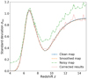 |
Fig. 7. Local variance of the brightness temperature maps of the M9 21cmFAST simulation, for a clean map (solid blue line), a map smoothed to SKA1-Low angular resolution for the optimistic case (bmax = 65 km, dashed orange line), and a noisy map (dash-dotted green line). See text for details. |
Subtracting the two local variances, we obtain the results shown as the dotted line in Fig. 7 and refer to these as the corrected results in the following. In these corrected results, the noise bias has been removed, and the measured local variance is much closer to the local variance values obtained from the clean smoothed maps than from the uncorrected one. Although Eq. (14) is an approximation and overlooks potential correlations between the cosmological signal and the noise within a slice, the good match between σloc derived from clean maps and from corrected maps shows that their contribution is sufficiently small to justify this approximation. In the optimistic case, the noise variance, and the associated fluctuations at high redshift, still remain but the location of the maximum of the local variance can be recovered.
In Fig. 8, we show the local variance of the noisy maps obtained in the optimistic and pessimistic case for the three 21cmFAST simulations: the three models can still be distinguished by the amplitude of σloc when analysing noisy maps. We see that the smoothing due to the coarser angular resolution of the pessimistic case leads to a decrease in the signal. However, a lower angular resolution is also equivalent to a lower noise variance (see Eq. (13)), such that the local variance of the noise does not exceed 0.02 mK, and the signal-to-noise ratio is around 50 during the bulk of reionisation. Therefore, we can recover the location of the maximum as well as the shape of the signal very well. Additionally, the ratio of the local variance maxima from one rsage model to another is well preserved: adding observational effects does not alter the ability of the local variance to differentiate between reionisation models.
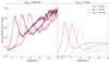 |
Fig. 8. Local variance of the 21 cm brightness temperature maps of the 21cmFAST simulations, after applying telescope resolution smoothing and adding telescope noise, for an optimistic case (bmax = 65 km, left), and a pessimistic case (bmax = 2 km, right). The shaded regions correspond to the standard deviation of the σloc values obtained from 100 different realisations of the thermal noise. |
Indeed, we fit a parabola y(z)/σ0 = σmax/σ0 − (z − zmax)2, with σ0 = 1mK, to the local variance data points of our M9 simulation, on a redshift range 6.8 ≤ z ≤ 7.5, for clean, noisy and corrected values. In this expression, zmax is the redshift when the maximum of the local variance is reached, and σmax its amplitude. To estimate the corresponding uncertainties, we derive the standard deviation of the local variance by running 21cmFAST for identical physical and numerical parameters but 200 different random seeds, which is equivalent to computing 200 different realisations of the simulation. We find that, in the optimistic case, the recovered amplitude is identical for all three data sets, giving σmax = (0.82 ± 0.24) mK at the 95% confidence level. The location of the peak is slightly shifted towards larger redshifts for noisy data: we find  for both the optimistic and the pessimistic case, which is close to the value obtained for clean data (
 ), and most importantly, within the size of a redshift bin (the redshift step between two snapshots is Δz = 0.2).
Accounting for the thermal noise is not sufficient to claim that our statistic will keep its characteristics and constraining power when analysing observed data, as we have not considered the impact of foreground avoidance or removal on our results. Nevertheless, Harker et al. (2009) have found that one-point statistics are quite robust against the details of foreground fitting. In contrast, Petrovic & Oh (2011) have shown that foreground cleaning can significantly distort the one-point PDF by smoothing out its bi-modal structure4. This will not be an issue for our local variance analysis, since, in contrast to the 3D pixel distribution, the distribution of mean values is smoothed by the averages along the frequency direction, and therefore not bi-modal. Additionally, foreground cleaning will reduce the contrast between neutral and ionised regions while maintaining the topology of the map, so that the distribution of means values and the variance within individual slices should be maintained. Finally, and similarly to our thermal noise analysis, it might be possible to remove the effects of foreground removal from the measured local variance, if we can characterise the statistical properties of foreground residuals sufficiently well. Analysing the contribution of the different k-modes to our local variance signal (for details see Appendix D), we find small k-modes, for which foreground contamination is the largest, to contribute the most. We therefore discard the possibility of using foreground avoidance to derive the local variance from 21 cm data. Instead foreground modelling and subtraction (Chapman et al. 2013; Mertens et al. 2018; Hothi et al. 2021) or using machine-learning techniques to reconstruct the signal lost in the foreground wedge (Gagnon-Hartman et al. 2021), should be preferred. We keep a thorough analysis of the impact of foreground removal on the local variance for future work.
4.4. Cross-correlations between slices
In the previous sections, we have discussed the auto-correlations of slices within a simulation box. Another option is to analyse the cross-correlations between the average values of slices separated by a given distance s. This approach is similar to what has been done for the one-point PDF in Barkana & Loeb (2008), Ichikawa et al. (2010) and Gluscevic & Barkana (2010). For the M9 simulation, we compute the following variance, to which we refer to as the cross variance:
 (15)
(15)
where μ(k, z) is the average of the kth slice and μ(k + is, z) is the average of the (k + is)th slice with s = i × Δx being the distance in Mpc separating them. This cross variance is equivalent to computing the 1D 2-point correlation function of the distribution of the means of slices. An example for the cross-correlation between slices at z = 7.2 and  is shown in Fig. 9 for the density, ionisation and brightness temperature fields of the M9 simulation. We find that, for all fields, the cross correlation is maximal at s = 0, corresponding to auto-correlations, and decreases towards larger separations until it reaches negative values. A similar evolution was observed in Muñoz & Cyr-Racine (2021). We note that the values presented in the figure are normalised by V(z, 0). Raw values are of the order of ∼10−6 for the ionisation field and 0.1 mK2 for the 21 cm brightness temperature field.
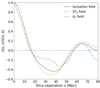 |
Fig. 9. Cross-correlations between the average values of two slices cut through the M9 simulation and separated by a distance s, for the snapshot corresponding to z = 7.2, normalised by the value at s = 0. Results are presented for the ionisation field (solid blue line) and the 21 cm brightness temperature field (dashed orange line). |
We compute the cross variance for all snapshots available in the M9 simulation. Interestingly, while the amplitude of V(z, s) changes with redshift for the density field, its shape remains constant, and so does V(z, s)/V(z, 0). Initially, the cross variance of the δTb field has the same behaviour as the density field, until the box is about 10% ionised. For the same redshifts, the scale at which V(z, s) derived from the ionisation field becomes zero, s0(z), remains around 15 Mpc. At  , the δTb field mostly follows xH I and s0 starts increasing. The maximum of s0 is reached at
  . At this time, all ionised regions have percolated and the variance drops to zero. If we compare results between the three 21cmFAST simulations, we find their cross variances to be very similar, when they are measured at the same stage in the reionisation process. For this reason, it is not possible to use the cross variance to constrain reionisation physics. We keep a thorough investigation of these cross-correlations for future work.
The value of s0 at z = 7.2 is equivalent to about 1 MHz, which also corresponds to the order of magnitude of the coherency length of the cosmological 21 cm signal during reionisation. While foregrounds are expected to have a much larger coherency length (∼50 − 100 Mpc), noise has a zero coherency length (Santos et al. 2005; Mertens et al. 2018). These differences provide the basis for statistical 21 cm signal separation via Gaussian Process Regression analysis (GPR, Mertens et al. 2018), where the different components of the observed signal are modelled in order to remove foregrounds from the 21 cm observations. Because their coherency length is much larger than the frequency bandwidth, the cosmological 21 cm signal and foregrounds measured in two consecutive frequency channels (or, here, slices) should be almost identical and, when subtracting measurements in these two channels, only the uncorrelated thermal noise should remain. In Patil et al. (2016), the authors use this technique to estimate the noise properties and remove noise from LOFAR data. Indeed, in contrast to foregrounds and cosmological signal, the thermal noise is found to be uncorrelated, even with a frequency separation as small as 0.2 MHz. Therefore, the difference between two Stokes I images in two consecutive frequency channels, after removing bright sources, will be dominated by thermal noise. Estimating the noise properties with this method leads to higher noise levels than when using Stokes V. The authors state that this excess noise is due to their calibration with an incomplete model. However, since this excess noise is uncorrelated between different observations, multiplying different observations will decrease the effective noise.
5. Discussion and conclusion
In this paper, we have presented a novel first-order statistics, the local variance σloc, which can be used to constrain the history and morphology of reionisation.
The local variance corresponds to the variance of the distribution of means of slices taken along an axis in a simulation, or along the frequency direction of observations, if the channel width is sufficiently narrow. At a fixed global ionisation level, the amplitude of the local variance of the ionisation field  is a tracer of the size of ionised regions: it is higher for an ionisation field showing a few large ionised regions, that is when ionising sources are more scarce but more efficient at ionising. For a field made of many small ionised regions, as it arises when low-mass sources are the main drivers of reionisation for example, the local variance will be smaller. In future work, we will investigate in more details how the local variance can constrain the physical properties of early galaxies. Additionally, the filling fraction for which the local variance reaches its maximum is mostly sensitive to the large-scale structure of the ionisation field during reionisation. It will be reached when both ionised and neutral regions are the largest, which occurs when approximately 60% of the box is ionised. We have found that a more biased ionising emissivity distribution (that is fewer sources with higher ionising emissivities opposed to many sources with lower ionising emissivities) results in the maximum local variance being reached earlier in the reionisation process, that is at a lower ionisation fraction
  . Finally, when applying our novel statistics to the differential 21 cm brightness temperature fields, the redshift-evolution of
  exhibits a characteristic shape that traces the reionisation history of the sky patch observed. Before the onset of reionisation,
  traces the correlations within the density field, but becomes sensitive to the ionisation morphology as a rising number of ionised regions emerge and grow.
We have shown that  is robust against thermal noise and angular resolution pollution when conducting 1000 hrs observations with SKA1-Low. For high angular resolution – corresponding to a maximum baseline of 65 km, the smoothing due to limited angular resolution has no impact on the local variance but the thermal noise adds amplitude and fluctuations to the signal. We have found that if the statistical properties of the noise are sufficiently known, the thermal noise contribution can be removed from the measured signal, and only the thermal noise fluctuations are conserved. For lower angular resolution – corresponding to a maximum baseline of 2 km, the smoothing leads to a decrease in the variance of the field and the noise level. In both cases, we can recover the maximum of the local variance as well as differentiate between the different reionisation models investigated in this work from noisy 21 cm maps. We expect this result to hold even after foreground removal. Indeed, σloc changes only weakly when the one-point PDF is altered by foreground removal (Petrovic & Oh 2011). A detailed analysis of the impact of foreground removal on the local variance will be the focus of future work. In conclusion, local variance data will enable the recovery of the reionisation history in a model-free fashion, as well as the constraint of astrophysical parameters related to the physical properties of early galaxies. Applying our local variance statistics to measurements would consist of obtaining the reionisation midpoint of a statistical sample of small fields of view, which are either obtained by dividing a larger observational window into smaller areas or by performing a series of different observations, and combining these ‘local’ reionisation midpoints to estimate a global reionisation midpoint. In this work, for computational reasons, individual observations have been represented by the different slices in a single coeval cube.
We note that other sample shapes could have been considered instead of slices. For example, Giri et al. (2019) consider the power spectrum measured in sub-cubes of a simulation. Since observational data cubes will consist of slices at different (but gradually increasing) frequencies, our findings can be easier translated to the results from observations. Alternatively, Bittner & Loeb (2011) consider the distribution of means measured across beams drawn along the frequency direction, and one could also consider the mean of sub-cubes in the entire coeval simulation box. Preliminary calculations have shown that the local variances of both shapes suffer from the same drawbacks, that is their strong dependency on the simulation size and resolution, but yield very similar results.
As the integral of the power spectrum, the local variance inherently includes the same information about the underlying reionisation field. However, it will be less affected by observational limitations. For example, because it is measured at a given frequency, we can avoid frequency channels contaminated by radio frequency interference (RFI). In addition, extracting patches of sky smaller than the total field of view of the 21 cm observations can eliminate survey boundary effects coming from tapering. In Appendix E, we find the local variance to be more robust to thermal noise than the power spectrum, except on scales k < 0.5 Mpc−1, where the cosmological signal is expected to be swamped by foregrounds.
Depending on the reionisation scenario, the 21 cm local variance can reach values as high as 1 mK. However, this value will naturally decrease as larger field of views or higher frequency resolutions are considered. While in this work, large values of the sample variance are desired, it has previously been considered an issue, as it represents an obstacle for a precise estimate of the 21 cm global signal or power spectrum and, in turn, of astrophysical parameters. Muñoz & Cyr-Racine (2021) proposed a way of quickly estimating the sample variance when measuring the 21 cm global signal as a function of its derivative with respect to redshift. Considering a simulation as big as L = 1.8 Gpc, Muñoz & Cyr-Racine (2021) find a maximum sample variance of σ21 ∼ 0.6 mK at z = 16.8. In parallel, Kaur et al. (2020) estimated that a simulation needs to be at least 200 − 300 Mpc wide to obtain a bias-free 21 cm power spectrum on scales of −1.2 < log k/Mpc−1 < 0. In contrast to other estimators, the local variance uses sample variance, often considered an observational bias, to our benefit. Looking for optimal observational strategies allowing a maximum amplitude of the local variance, while minimising its error bars, in order to offer reliable constraints, will be the focus of future work.
Available at https://github.com/21cmfast/21cmFAST
The definition of the 2-PCF yields
 (6)
(6)
such that, for an isotropic and homogeneous field,
 (7)
(7)
Because we use coeval cubes, we assume that the redshift does not change from one slice to the next. This is a reasonable assumption because of the relatively small size of the box (L = 160 Mpc).
Ionised pixels form a Dirac peak centred on zero, whilst warm pixels are distributed more evenly.
Acknowledgments
The authors thank the referee for useful comments on this manuscript, which helped improve its overall quality. They also thank Catherine A. Watkinson, Ian Hothi, Adrian C. Liu and Jordan Mirocha for their input on a draft version of this paper; as well as Jacob Seiler for providing the rsage simulations. AG and JP acknowledge financial support from the European Research Council under ERC grant number StG-638743 (“FIRSTDAWN”). AG’s work was additionally supported by the McGill Astrophysics Fellowship funded by the Trottier Chair in Astrophysics, as well as the Canadian Institute for Advanced Research (CIFAR) Azrieli Global Scholars program. AH acknowledges support from the European Research Council’s starting grant ERC StG-717001 (“DELPHI”). The idea of this work was developed thanks to visits between the authors of this paper, partly funded by the Leids Kerkhoven-Bosscha Fonds (LKBF). This research made use of astropy, a community-developed core Python package for astronomy (Astropy Collaboration 2013, 2018); matplotlib, a Python library for publication quality graphics (Hunter 2007); and of scipy, a Python-based ecosystem of open-source software for mathematics, science, and engineering (Jones et al. 2001) – including numpy (Oliphant 2006).
References
- Astropy Collaboration (Robitaille, T. P., et al.) 2013, A&A, 558, A33 [NASA ADS] [CrossRef] [EDP Sciences] [Google Scholar]
- Astropy Collaboration (Price-Whelan, A. M., et al.) 2018, AJ, 156, 123 [Google Scholar]
- Bañados, E., Venemans, B. P., Mazzucchelli, C., et al. 2018, Nature, 553, 473 [NASA ADS] [CrossRef] [Google Scholar]
- Banet, A., Barkana, R., Fialkov, A., & Guttman, O. 2021, MNRAS, 503, 1221 [NASA ADS] [CrossRef] [Google Scholar]
- Barkana, R., & Loeb, A. 2008, MNRAS, 384, 1069 [NASA ADS] [CrossRef] [Google Scholar]
- Beardsley, A. P., Morales, M. F., Lidz, A., Malloy, M., & Sutter, P. M. 2015, ApJ, 800, 128 [NASA ADS] [CrossRef] [Google Scholar]
- Bittner, J. M., & Loeb, A. 2011, JCAP, 2011, 038 [Google Scholar]
- Bouwens, R. J., Illingworth, G. D., Oesch, P. A., et al. 2015, ApJ, 803, 34 [Google Scholar]
- Braun, R., Bonaldi, A., Bourke, T., Keane, E., & Wagg, J. 2019, ArXiv e-prints [arXiv:1912.12699] [Google Scholar]
- Chapman, E., & Jelić, V. 2019, in The Cosmic 21-cm Revolution, 2514–3433 (IOP Publishing), 6 [Google Scholar]
- Chapman, E., Abdalla, F. B., Bobin, J., et al. 2013, MNRAS, 429, 165 [NASA ADS] [CrossRef] [Google Scholar]
- Chiang, C.-T., Wagner, C., Sánchez, A. G., Schmidt, F., & Komatsu, E. 2015, JCAP, 2015, 028 [CrossRef] [Google Scholar]
- Ciardi, B., & Madau, P. 2003, ApJ, 596, 1 [NASA ADS] [CrossRef] [Google Scholar]
- Croton, D. J., Stevens, A. R. H., Tonini, C., et al. 2016, ApJS, 222, 22 [Google Scholar]
- Datta, K. K., Ghara, R., Majumdar, S., et al. 2016, JApA, 37, 27 [NASA ADS] [Google Scholar]
- DeBoer, D. R., Parsons, A. R., Aguirre, J. E., et al. 2017, PASP, 129, 045001 [NASA ADS] [CrossRef] [Google Scholar]
- Furlanetto, S. R., Zaldarriaga, M., & Hernquist, L. 2004, ApJ, 613, 1 [NASA ADS] [CrossRef] [Google Scholar]
- Gagnon-Hartman, S., Cui, Y., Liu, A., & Ravanbakhsh, S. 2021, MNRAS, 504, 4716 [NASA ADS] [CrossRef] [Google Scholar]
- Giri, S. K., Mellema, G., & Ghara, R. 2018, MNRAS, 479, 5596 [NASA ADS] [CrossRef] [Google Scholar]
- Giri, S. K., D’Aloisio, A., Mellema, G., et al. 2019, JCAP, 2019, 058 [Google Scholar]
- Gluscevic, V., & Barkana, R. 2010, MNRAS, 408, 2373 [NASA ADS] [CrossRef] [Google Scholar]
- Gorce, A., & Pritchard, J. R. 2019, MNRAS, 489, 1321 [NASA ADS] [CrossRef] [Google Scholar]
- Gorce, A., Douspis, M., Aghanim, N., & Langer, M. 2018, A&A, 616, A113 [EDP Sciences] [Google Scholar]
- Greig, B., Trott, C. M., Barry, N., et al. 2021, MNRAS, 500, 5322 [Google Scholar]
- Harker, G. J. A., Zaroubi, S., Thomas, R. M., et al. 2009, MNRAS, 393, 1449 [NASA ADS] [CrossRef] [Google Scholar]
- Heneka, C., & Mesinger, A. 2020, MNRAS, 496, 581 [NASA ADS] [CrossRef] [Google Scholar]
- Hothi, I., Chapman, E., Pritchard, J. R., et al. 2021, MNRAS, 500, 2264 [Google Scholar]
- Hunter, J. D. 2007, Comput. Sci. Eng., 9, 90 [NASA ADS] [CrossRef] [Google Scholar]
- Hutter, A. 2018a, CIFOG: Cosmological Ionization Fields frOm Galaxies [Google Scholar]
- Hutter, A. 2018b, MNRAS, 477, 1549 [Google Scholar]
- Hutter, A., Watkinson, C. A., Seiler, J., et al. 2020, MNRAS, 492, 653 [CrossRef] [Google Scholar]
- Ichikawa, K., Barkana, R., Iliev, I. T., Mellema, G., & Shapiro, P. R. 2010, MNRAS, 406, 2521 [NASA ADS] [CrossRef] [Google Scholar]
- Jones, E., Oliphant, T., & Peterson, P. 2001, SciPy: Open source scientific tools for Python [Google Scholar]
- Kakiichi, K., Majumdar, S., Mellema, G., et al. 2017, MNRAS, 471, 1936 [NASA ADS] [CrossRef] [Google Scholar]
- Kaur, H. D., Gillet, N., & Mesinger, A. 2020, MNRAS, 495, 2354 [NASA ADS] [CrossRef] [Google Scholar]
- Kittiwisit, P., Bowman, J. D., Jacobs, D. C., Beardsley, A. P., & Thyagarajan, N. 2018, MNRAS, 474, 4487 [NASA ADS] [CrossRef] [Google Scholar]
- Koopmans, L., Pritchard, J., Mellema, G., et al. 2015, Advancing Astrophysics with the Square Kilometre Array, AASKA14, 1 [NASA ADS] [Google Scholar]
- Liu, A., & Shaw, J. R. 2020, PASP, 132, 062001 [NASA ADS] [CrossRef] [Google Scholar]
- Majumdar, S., Pritchard, J. R., Mondal, R., et al. 2018, MNRAS, 476, 4007 [NASA ADS] [CrossRef] [Google Scholar]
- Malloy, M., & Lidz, A. 2013, ApJ, 767, 68 [NASA ADS] [CrossRef] [Google Scholar]
- Mangena, T., Hassan, S., & Santos, M. G. 2020, MNRAS, 494, 600 [NASA ADS] [CrossRef] [Google Scholar]
- McGreer, I. D., Mesinger, A., & D’Odorico, V. 2015, MNRAS, 447, 499 [NASA ADS] [CrossRef] [Google Scholar]
- McQuinn, M., Lidz, A., Zahn, O., et al. 2007, MNRAS, 377, 1043 [NASA ADS] [CrossRef] [Google Scholar]
- Mellema, G., Iliev, I. T., Pen, U.-L., & Shapiro, P. R. 2006, MNRAS, 372, 679 [NASA ADS] [CrossRef] [Google Scholar]
- Mertens, F. G., Ghosh, A., & Koopmans, L. V. E. 2018, MNRAS, 478, 3640 [NASA ADS] [Google Scholar]
- Mesinger, A., & Furlanetto, S. 2007, ApJ, 669, 663 [Google Scholar]
- Mesinger, A., Furlanetto, S., & Cen, R. 2011, MNRAS, 411, 955 [Google Scholar]
- Muñoz, J. B., & Cyr-Racine, F.-Y. 2021, Phys. Rev. D, 103, 023512 [Google Scholar]
- Oliphant, T. 2006, NumPy: A guide to NumPy (USA: Trelgol Publishing) [Google Scholar]
- Pagano, M., & Liu, A. 2020, MNRAS, 498, 373 [NASA ADS] [CrossRef] [Google Scholar]
- Patil, A. H., Zaroubi, S., Chapman, E., et al. 2014, MNRAS, 443, 1113 [NASA ADS] [CrossRef] [Google Scholar]
- Patil, A. H., Yatawatta, S., Zaroubi, S., et al. 2016, MNRAS, 463, 4317 [NASA ADS] [CrossRef] [Google Scholar]
- Petrovic, N., & Oh, S. P. 2011, MNRAS, 413, 2103 [NASA ADS] [CrossRef] [Google Scholar]
- Planck Collaboration I. 2016, A&A, 594, A1 [NASA ADS] [CrossRef] [EDP Sciences] [Google Scholar]
- Planck Collaboration Int. XLVII. 2016, A&A, 596, A108 [NASA ADS] [CrossRef] [EDP Sciences] [Google Scholar]
- Pritchard, J. R., & Loeb, A. 2012, Rep. Prog. Phys., 75 [Google Scholar]
- Robertson, B. E., Ellis, R. S., Furlanetto, S. R., & Dunlop, J. S. 2015, ApJ, 802, L19 [Google Scholar]
- Santos, M. G., Cooray, A., & Knox, L. 2005, ApJ, 625, 575 [NASA ADS] [CrossRef] [Google Scholar]
- Seiler, J., Hutter, A., Sinha, M., & Croton, D. 2019, MNRAS, 1578 [Google Scholar]
- Shimabukuro, H., Yoshiura, S., Takahashi, K., Yokoyama, S., & Ichiki, K. 2016, MNRAS, 458, 3003 [NASA ADS] [CrossRef] [Google Scholar]
- Watkinson, C. A., & Pritchard, J. R. 2014, MNRAS, 443, 3090 [NASA ADS] [CrossRef] [Google Scholar]
- Watkinson, C. A., Giri, S. K., Ross, H. E., et al. 2019, MNRAS, 482, 2653 [NASA ADS] [CrossRef] [Google Scholar]
- Zahn, O., Lidz, A., McQuinn, M., et al. 2007, ApJ, 654, 12 [NASA ADS] [CrossRef] [Google Scholar]
Appendix A: Local variance of the δTb field
In the following we consider the 21 cm brightness temperature field to be the direct product of the neutral hydrogen H I and the overdensity  fields,
![Mathematical equation: $$ \begin{aligned} \delta T_{\rm b}(\boldsymbol{x}) = x_{\rm {\text{ H}}{\small {{\text{ I}}}}}(\boldsymbol{x}) \times \left[1+\delta _{\rm b}(\boldsymbol{x})\right]. \end{aligned} $$](/articles/aa/full_html/2021/09/aa40515-21/aa40515-21-eq72.gif) (A.1)
(A.1)
If we consider the kth slice along the frequency direction in the simulation, we yield from the previous equation
![Mathematical equation: $$ \begin{aligned} \delta T_{\rm b,loc}(k) = E[\delta T_{\rm b}(k)] = E \left[ x_{\rm {\text{ H}}{\small {{\text{ I}}}}}(k) \times (1+\delta _{\rm b}(k)) \right], \end{aligned} $$](/articles/aa/full_html/2021/09/aa40515-21/aa40515-21-eq73.gif) (A.2)
(A.2)
where E is the expectation value, δTb, loc(k) is the mean of the 21 cm field of the slice, xH I(k) its 2D H I field and δb(k) its 2D overdensity field. Since these two fields are correlated, equation A.2 can be reformulated as
![Mathematical equation: $$ \begin{aligned} \begin{aligned} \delta T_{\rm b,loc}(k) = \bar{x}_{\rm {\text{ H}}{\small {{\text{ I}}}}}&(k) \times (1+\bar{\delta }_{\rm b}(k)) \\&+ \mathrm{Cov}\left[ x_{\rm {\text{ H}}{\small {{\text{ I}}}}}(k) \times (1+\delta _{\rm b}(k)) \right]. \end{aligned} \end{aligned} $$](/articles/aa/full_html/2021/09/aa40515-21/aa40515-21-eq74.gif) (A.3)
(A.3)
Then the local variance is the variance of the distribution of δTb, loc values. If we write  and
and ![Mathematical equation: $ Y=\mathrm{Cov}\left[ x_\mathrm{{\mathrm{H}\,\textsc{i}}}(k) \times (1+\delta_{\mathrm{b}}(k)) \right] $](/articles/aa/full_html/2021/09/aa40515-21/aa40515-21-eq76.gif) then
then
![Mathematical equation: $$ \begin{aligned} \begin{aligned} {{\sigma _{\rm loc}}}^2&= \mathrm{Var}(\delta T_{\rm b,loc}) \\&= 2\,\mathrm{Cov}(X,Y) + \mathrm{Var}X + \mathrm{Var}Y\\&= \mathrm{Cov}[\bar{x}_{\rm {\text{ H}}{\small {{\text{ I}}}}}^2, (1+\bar{\delta }_{\rm b})^2] + \left( \sigma _{\mathrm{loc},{\text{ H}}{\small {{\text{ I}}}}}^2 + \bar{x}_{\rm {\text{ H}}{\small {{\text{ I}}}}}^2 \right) \left( \sigma _{\mathrm{loc},\delta _b}^2 + 1 \right)\\&- \left[ \mathrm{Cov}[\bar{x}_{\rm {\text{ H}}{\small {{\text{ I}}}}}, (1+\bar{\delta }_{\rm b})] + \bar{x}_{\rm {\text{ H}}{\small {{\text{ I}}}}} \right]^2. \end{aligned} \end{aligned} $$](/articles/aa/full_html/2021/09/aa40515-21/aa40515-21-eq77.gif) (A.4)
(A.4)
These different elements are represented in Fig. A.1.
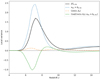 |
Fig. A.1. Contributions to the local variance of the 21 cm brightness temperature field in a 21cmFAST simulation. |
We see that the final shape of the local variance is mostly made of the variance of X, the product of the two local fields, and of the covariance of X and Y, which are both complicated objects difficult to interpret. However, as shown in Fig. 3, considering the local variances of xH I and 1 + δb, as well as their covariance, is sufficient to understand the redshift-evolution of  .
.
Appendix B: Tests on toy models
We generate toy models with dimensions equal to those of the rsage simulations, that is a comoving box length of L = 160 Mpc and 256 grid cells on each side. The initial field is a 3D neutral box filled with enough bubbles of radius Rinit to reach a filling fraction of  , which are then artificially grown by 1 cell in radius until a filling fraction of 100% is reached. We compute the local variance for each of the resulting boxes. Results can be seen in Fig. B.1 in comparison to a control test where ionised pixels are randomly distributed. We evolve the toy model boxes with different initial radii: a large Rinit will be equivalent to a higher mass threshold for ionising sources, that is an increasing Rinit will be equivalent to an increasing Mturn in 21cmFAST or transitioning from rsage fej via rsage const to rsage SFR. The difference to 21cmFAST and rsage is that ionised bubbles are randomly located, so the ionising sources are not clustered. Additionally, there are no new ionised regions throughout the process, since all the bubbles are initialised in the first field. Despite these differences, the shape of
  remains unchanged, and the maximum is still reached for a filling fraction of about 0.60:
  for the field with small bubbles, and
  for the field with large bubbles. Similarly to what has been seen from the 21cmFAST simulations, the simulation with the largest bubbles reaches on average its maximum local variance at smaller filling fractions.
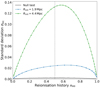 |
Fig. B.1. Local variance σloc for toy models with different starting radius. |
Appendix C: Dependence on box size and other limitations
Because the information contained in σloc is purely related to the sample variance, σloc will depend on the size of the box considered: the larger the box, the smaller the variance. In order to compare with the fields-of-views anticipated for upcoming 21 cm experiments, we ask what is the limiting size that allows us to differentiate between reionisation models with σloc. To do so, we generate a 21cmFAST simulation box for Mturn = 109 M⊙, side length L = 480 Mpc and cell size Δx = 0.625 Mpc, same as before. We divide this large simulation into sub-cubes of decreasing size, until a side length of L = 15 Mpc is reached (All sub-cubes have identical reionisation histories.). We compute the local variance obtained from the 21 cm brightness temperature fields of all sub-cubes and compare their values in Fig. C.1. The maximum signal is reached for the smallest box size, L = 15 Mpc, and reaches values as high as 5.5 mK, which is 10 times higher than the fiducial boxes we analysed in Sect. B. For all box sizes, we can locate a maximum signal at the same redshift, corresponding to 61% of global ionisation level. It decreases drastically with box size, according to
 (C.1)
(C.1)
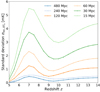 |
Fig. C.1. Evolution of the standard deviation of the xloc distributions for M9 simulations of decreasing side length but constant resolution. |
SKA1-Low has a field of view of 327 arcmin at nominal frequency of 110 MHz, which corresponds to L = 760, 840, 900, 940, and 970 Mpc at z = 5, 7, 9, 11 and 13, respectively. For such wide observational windows, the sample variance is weak: at z = 6, towards the end of reionisation, it will be about ∼0.25 mK. This relation is only valid at a time when about 60% of the IGM is ionised, which will correspond to different redshifts depending on the reionisation scenario. However, it will give the maximum amplitude of σloc and is therefore a useful choice, if we want to estimate the errors on 21 cm global signal measurements. Interestingly, it is about 10 times smaller than the one found by Muñoz & Cyr-Racine (2021) at z = 16.3, which confirms how dependent the amplitude of the local variance is on the physics of reionisation and on the reionisation stage it is computed at.
Additionally, we expect σloc to depend on the resolution of the simulation considered – or on the angular resolution of the telescope used. Indeed, Banet et al. (2021) already pointed out the impact of instrument resolution and smoothing on the one-point and differential PDF. The anticipated angular resolution of SKA1 at a nominal frequency of 110 MHz is expected to be 11 arcsec (Braun et al. 2019), that is between 0.45 and 0.55 Mpc on the redshift range 5 ≤ z ≤ 13. Running 21cmFAST for Mturn = 109 M⊙ and a fixed number of cells but an increasing resolution, from Δx = 0.5 Mpc to 3 Mpc, we find that an improved resolution enhances the local variance as structures are better resolved and the number of partially ionised regions decreases.
Finally, computing σloc requires to have a sufficient number of slices available: it is obvious from Fig. 2 that without a sufficient number of slices, the xloc distributions will be noisy and their variance σloc will not be reliable. For the M9 simulation, we find that 128 slices, so half of the box, will still provide satisfying results, while lower sample sizes make σloc unusable. However, thanks to the very high frequency resolution of SKA, anticipated to be 5.4 kHz at 110 MHz (Braun et al. 2019), we expect to observe a sufficient number of images at sufficiently close redshifts for σloc to give interesting results. This will be the focus of future work.
Appendix D: Mode contribution to the local variance
To estimate the impact of foregrounds on the local variance, we analyse the contribution of different k-modes to the σloc(z) signal. According to Eq. (11), the local variance is the integral over the power spectrum of the 1D distribution of the mean values along the line of sight and/or redshift direction Pμ(k). Hence, Pμ(k) is a direct measure of the contribution of each k-mode to the local variance: for the M9 simulation, we show Pμ(k) at z = 5 − 11 in Fig. D.1.
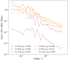 |
Fig. D.1. Evolution of the power spectrum of the 1D distribution of means along the redshift direction Pμ(k) of the M9 simulation, illustrating the contribution of Fourier modes to the local variance. |
First, and as expected, the evolution of the global amplitude of Pμ(k) recovers the redshift-evolution of the local variance and, in particular, its maximum around z ∼ 7. Additionally, we see that the low-k modes are the ones contributing the most to the local variance signal as Pμ(k) decreases with increasing k values following Pμ(k) ∝ k−2 approximately at all redshifts. This confirms our findings in Sect. 4.2, that the local variance, and in particular the location of its maximum, is sensitive to the ionisation morphology on large scales. Furthermore, because foreground corruption is larger for small k-modes, this result shows that foreground avoidance is likely to diminish the reionisation signal in the local variance of the 21 cm signal. Other possibilities should be considered, such as foreground removal (Chapman et al. 2013; Hothi et al. 2021) or machine-learning techniques to reconstruct the wedge (Gagnon-Hartman et al. 2021).
Appendix E: Performance comparison with the power spectrum
As an integral of the power spectrum, the variance – local or not, inherently encompasses the same information. However, as we explain in this Section, we expect the local variance o be less affected by observational limitations than the power spectrum.
In Sect. 2 we have mentioned that, if this work was based on the analysis of coeval cubes for computational reasons, this approach is not directly transferable to 21 cm observations since different slices along the observed light cone correspond to different redshifts. Instead, we would consider a wide field-of-view at a given frequency (or redshift), and divide it into sub-patches – an approach already imagined in Giri et al. (2019). Comparing the means of these sub-patches is then equivalent to comparing the means of slices of a coeval cube. Therefore, one is able to pick sub-patches in a way that avoids survey boundary effects, which are a common problem of power spectrum estimations. Additionally, since the signal is measured for a given frequency bin, one can conveniently choose what frequency is considered, and in particular avoid frequency bands dominated by, for example, radio-frequency interference (RFI).
We now perform a comparison of the robustness of the power spectrum and of the local variance to thermal noise. For every snapshot available from the M9 simulation, we generate 100 realisations of thermal noise fields and add them to the 21 cm brightness temperature field that is smoothed according to a maximum baseline of bmax = 2 km or 65 km. We choose a 21cmFAST simulation of box size of 50 Mpc for 100 pixels per side and set Mturn = 109 M⊙. We compute the three-dimensional power spectrum and the local variance of each of these 100 boxes, and take their standard deviation as the error due to noise for each estimator. The resulting relative error bars are shown in the left panels of Fig. E.1. We see that, thanks to σloc being the integral over all k-modes, the relative error of the σloc values remains constant over the redshift range, with values of ∼6% for the bmax = 65 km case. For bmax = 2 km, results are even better with relative errors lower than 1% for z ≥ 6 and lower than the relative error obtained for the power spectrum on all scales. This is not surprising, since Eq. (13) shows that the variance of the noise is inversely proportional to the angular resolution of the telescope and therefore smaller for our pessimistic case.
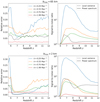 |
Fig. E.1. Relative error bars (left panel) and signal-to-noise ratio (right panel) obtained from measurements of the local variance and the 21 cm power spectrum with different realisations of the noise added to a 21cmFAST simulation. Two observational cases are considered: a maximum baseline of bmax = 65 km (upper panel), and one of bmax = 2 km (lower panel). |
Additionally, we compute the power spectrum and local variance of the 100 realisations of thermal noise alone and derive the signal-to-noise ratio (SNR) of the two estimators as ⟨Psmoothed(k)/Pnoise(k)⟩ and ⟨σlocsmoothed/σlocnoise⟩, respectively (see right panel in Fig. E.1). For the reasons mentioned above, the SNR values of the local variance for the bmax = 2 km case exceed those of the pessimistic baseline case. They are maximum at the redshifts where the local variance reaches its maximum (z ≃ 6.5 − 7.5), which is the range of greatest interest to us. For the pessimistic case, the SNR of the local variance is equal to ∼60 at z ≃ 6.5 − 7.5. We note that the SNR of the local variance is only smaller than the SNR of the power spectrum for small k-modes, k < 0.5 Mpc−1, but these modes are expected to be swamped by foregrounds.
In summary, we find that on average our estimator is more robust to thermal noise than the power spectrum, especially on scales k > 0.5 Mpc−1 that are key for deriving constraints on the reionisation morphology from observations.
All Figures
|
Fig. 1. Binary ionisation fields cut through the three rsage simulations (upper panels) and the three 21cmFAST runs (lower panels) described in Sect. 2 at |
| In the text | |
|
Fig. 2. Left panel: distribution of the ionisation levels of the N slices that can be carved out of the rsage const simulation along one direction. Each colour corresponds to one of 12 snapshots taken on the range 6.02 ≤ z ≤ 14.63, corresponding to different ionisation levels, represented as the solid vertical lines. Right panel: evolution of the standard deviations of each distribution with global reionisation history (blue solid line), compared to the standard deviation of the distribution of ionised pixels throughout the whole box (dashed line, divided by 10). |
| In the text | |
|
Fig. 3. Contributions to the local variance of the δTb field in the rsage const simulation (upper panel) and its reionisation history (lower panel). |
| In the text | |
|
Fig. 4. Evolution of the standard deviation on the distribution of means measured in the set of N slices that can be carved out of the ionisation fields of simulations along one direction with redshift (left panel) and ionisation level (middle panel). Right panel: corresponding reionisation histories. Results for the three rsage simulations (upper panels) and the three 21cmFAST runs (lower panels) are compared. |
| In the text | |
|
Fig. 5. Snapshots of the ionisation field at the maximum of the local variance for the M8, M9 and M10 simulations, corresponding to different redshifts and different ionisation levels: z = 8.4 and |
| In the text | |
|
Fig. 6. Local variance of the 21 cm brightness temperature fields from the rsage (upper panel) and 21cmFAST (lower panel) simulation, as a function of redshift. Vertical dotted lines show the ionisation midpoint of the simulation of the corresponding colour. |
| In the text | |
|
Fig. 7. Local variance of the brightness temperature maps of the M9 21cmFAST simulation, for a clean map (solid blue line), a map smoothed to SKA1-Low angular resolution for the optimistic case (bmax = 65 km, dashed orange line), and a noisy map (dash-dotted green line). See text for details. |
| In the text | |
|
Fig. 8. Local variance of the 21 cm brightness temperature maps of the 21cmFAST simulations, after applying telescope resolution smoothing and adding telescope noise, for an optimistic case (bmax = 65 km, left), and a pessimistic case (bmax = 2 km, right). The shaded regions correspond to the standard deviation of the σloc values obtained from 100 different realisations of the thermal noise. |
| In the text | |
|
Fig. 9. Cross-correlations between the average values of two slices cut through the M9 simulation and separated by a distance s, for the snapshot corresponding to z = 7.2, normalised by the value at s = 0. Results are presented for the ionisation field (solid blue line) and the 21 cm brightness temperature field (dashed orange line). |
| In the text | |
|
Fig. A.1. Contributions to the local variance of the 21 cm brightness temperature field in a 21cmFAST simulation. |
| In the text | |
|
Fig. B.1. Local variance σloc for toy models with different starting radius. |
| In the text | |
|
Fig. C.1. Evolution of the standard deviation of the xloc distributions for M9 simulations of decreasing side length but constant resolution. |
| In the text | |
|
Fig. D.1. Evolution of the power spectrum of the 1D distribution of means along the redshift direction Pμ(k) of the M9 simulation, illustrating the contribution of Fourier modes to the local variance. |
| In the text | |
|
Fig. E.1. Relative error bars (left panel) and signal-to-noise ratio (right panel) obtained from measurements of the local variance and the 21 cm power spectrum with different realisations of the noise added to a 21cmFAST simulation. Two observational cases are considered: a maximum baseline of bmax = 65 km (upper panel), and one of bmax = 2 km (lower panel). |
| In the text | |
Current usage metrics show cumulative count of Article Views (full-text article views including HTML views, PDF and ePub downloads, according to the available data) and Abstracts Views on Vision4Press platform.
Data correspond to usage on the plateform after 2015. The current usage metrics is available 48-96 hours after online publication and is updated daily on week days.
Initial download of the metrics may take a while.