| Issue |
A&A
Volume 678, October 2023
|
|
|---|---|---|
| Article Number | A86 | |
| Number of page(s) | 16 | |
| Section | Stellar structure and evolution | |
| DOI | https://doi.org/10.1051/0004-6361/202347145 | |
| Published online | 10 October 2023 | |
Star-disk interactions in the strongly accreting T Tauri star S CrA N⋆
1
Univ. Grenoble Alpes, CNRS, IPAG, 38000 Grenoble, France
e-mail: This email address is being protected from spambots. You need JavaScript enabled to view it.
2
Departamento de física, Universidade Federal de Minas Gerais, Belo Horizonte, MG 31270-901, Brazil
3
University of Tartu, Faculty of Science and Technology, Tartu Observatory, 51003 Tartu, Estonia
4
Department of Physics and Astronomy, Uppsala University, Box 516 75120 Uppsala, Sweden
5
Science Division, Directorate of Science, European Space Research and Technology Centre (ESA/ESTEC), Keplerlaan 1, 2201 AZ Noordwijk, The Netherlands
Received:
9
June
2023
Accepted:
3
August
2023
Abstract
Context. Classical T Tauri stars are thought to accrete material from their surrounding protoplanetary disks through funnel flows along their magnetic field lines. The classical T Tauri stars with high accretion rates (∼10−7 M⊙ yr−1) are ideal targets for testing this magnetospheric accretion scenario in a sustained regime.
Aims. We constrained the accretion-ejection phenomena around the strongly accreting northern component of the S CrA young binary system (S CrA N) by deriving its magnetic field topology and its magnetospheric properties, and by detecting ejection signatures, if any.
Methods. We led a two-week observing campaign on S CrA N with the ESPaDOnS optical spectropolarimeter at the Canada-France-Hawaii Telescope. We recorded 12 Stokes I and V spectra over 14 nights. We computed the corresponding least-squares deconvolution (LSD) profiles of the photospheric lines and performed Zeeman-Doppler imaging (ZDI). We analyzed the kinematics of noticeable emission lines, namely He I λ5876 and the first four lines of the Balmer series, which are known to trace the accretion process.
Results. We found that S CrA N is a low-mass (0.8 M⊙) young (∼1 Myr) and fully convective object exhibiting strong and variable veiling (with a mean value of 7 ± 2), which suggests that the star is in a strong accretion regime. These findings could indicate a stellar evolutionary stage between Class I and Class II for S CrA N. We reconstructed an axisymmetric large-scale magnetic field (∼70% of the total energy) that is primarily located in the dipolar component, but has significant higher poloidal orders. From the narrow emission component radial velocity curve of He I λ5876, we derived a stellar rotation period of P* = 7.3 ± 0.2 days. We found a magnetic truncation radius of ∼2 R* which is significantly closer to the star than the corotation radius of ∼6 R*, suggesting that S CrA N is in an unstable accretion regime. That the truncation radius is quite smaller than the size of the Brγ line emitting region, as measured with the GRAVITY interferometer (∼8 R*), supports the presence of outflows, which is nicely corroborated by the line profiles presented in this work.
Conclusions. The findings from spectropolarimetry are complementary to those provided by optical long-baseline interferometry, allowing us to construct a coherent view of the innermost regions of a young, strongly accreting star. The strong and complex magnetic field reconstructed for S CrA N is inconsistent with the observed magnetic signatures of the emission lines associated with the postshock region, however. We recommend a multitechnique synchronized campaign of several days to place more constrains on a system that varies on a timescale of about one day.
Key words: stars: variables: T Tauri / Herbig Ae/Be / stars: individual: S CrA N / stars: magnetic field / techniques: spectroscopic / techniques: polarimetric / accretion / accretion disks
PI (Perraut) Program 18AF12. Based on observations obtained at the Canada-France-Hawaii Telescope (CFHT) which is operated by the National Research Council of Canada, the Institut National des Sciences de l’Univers of the Centre National de la Recherche Scientifique of France, and the University of Hawaii.
© The Authors 2023
 Open Access article, published by EDP Sciences, under the terms of the Creative Commons Attribution License (https://creativecommons.org/licenses/by/4.0), which permits unrestricted use, distribution, and reproduction in any medium, provided the original work is properly cited.
This article is published in open access under the Subscribe to Open model. This email address is being protected from spambots. You need JavaScript enabled to view it. to support open access publication.
1. Introduction
Protoplanetary disks are gas- and dust-rich regions that are mostly constituted of hydrogen and helium gas. A small fraction of their content is in dust grains. As the reservoir from which matter is accreted onto the star and planets are built, protoplanetary disks set the initial conditions for planet formation. In the innermost regions of these disks, accretion flows, winds, and outflows are essential for controlling angular momentum, altering the gas content, and driving the dynamics of the gas (Alexander et al. 2014). While they are key elements for understanding the disk dynamics and its evolution locally and globally, the physical structure, the exact nature of the processes acting in these inner regions, and their interplay are still poorly constrained and not well understood.
Classical T Tauri stars (CTTS) are young suns (< 2 M⊙) that still accrete from their surrounding disk. The most commonly accepted scenario is that accretion is funnelled by the stellar magnetic field (Hartmann et al. 2016; Bouvier et al. 2007), which is strong enough to truncate the circumstellar disk at a few stellar radii from the central star. This magnetic field drives the ionized gas of the inner disk that falls onto the central object, and it forms shocks and hot spots at high latitudes on the stellar surface (Camenzind 1990; Koenigl 1991; Espaillat 2022). These phenomena shape many properties of the accreting objects and can be investigated by spectroscopy, spectropolarimetry, and photometry because their host stars exhibit excess continuum emission in the optical and near-infrared ranges, hot and cold spots, and broad, intense, and variable emission lines in the visible and near-infrared ranges (e.g., Alencar et al. 2012, 2018; Sousa et al. 2021, 2023).
The accretion regime depends on the large-scale magnetic field strength (i.e., usually a dipole), the angle between the dipolar magnetic field and stellar rotation axes, and the mass accretion rate (Kulkarni & Romanova 2008; Blinova et al. 2016). It can be either stable, when it occurs through two funnels, one per hemisphere, or unstable, when several equatorial tongues penetrate the stellar magnetosphere. These tongues are transient on timescales of the stellar rotation period and can coexist with stable accretion funnels (Kulkarni & Romanova 2008; Pantolmos et al. 2022). The transition between these regimes strongly depends on the mass accretion rate: unstable accretion is expected to be observed mostly in strong accretors rather than in low accretors (Blinova et al. 2016). Strong accretors allow us to probe a different accretion regime through which all low-mass stars are expected to pass during their early pre-main-sequence (PMS) evolution as they move away from the protostellar phase (Baraffe et al. 2017). Strong accretors have been poorly explored so far because their variablility in the optical domain complicates their spectral analysis.
Until recently, the structure of the magnetosphere has mostly been probed through indirect observations through measurements of the magnetic field strength and topology (Donati et al. 1997), and through mass accretion rate estimates (Manara et al. 2021; Alcalá et al. 2021). The drastic improvement in the sensitivity of optical long-baseline interferometers has opened a new promising way to probe the interaction between the young stars and their inner disks. The K-band interferometric beam-combiner GRAVITY1 at the very large telescope interferometer (VLTI; GRAVITY Collaboration 2017a) enables resolving the Br γ line emitting region spatially for a few T Tauri stars (GRAVITY Collaboration 2023). Combined with spectropolarimetry, this appears very promising because it allows comparing the size of the Br γ line emitting region with that of the magnetosphere derived by spectropolarimetry, and thus investigating the accretion-ejection processes at the (sub-)astronomical unit scale (Bouvier et al. 2020; GRAVITY Collaboration 2020, 2023).
With the aim of studying the peculiar accretion regime of a strong accretor through complementary observing techniques, we focus our work on the north component of the young binary system S Coronae Australis (S CrA N) because it is one of the strongest accretors of the GRAVITY T Tauri sample (̇M ∼ 10−7 M⊙ yr−1; Gahm et al. 2018; Sullivan et al. 2019). To complete the GRAVITY data set and better understand the accretion-ejection phenomena, we have conducted an observing campaign with the optical echelle spectropolarimetric device for the observation of stars (ESPaDOnS).
The components of the T Tauri binary system S CrA are coeval (Gahm et al. 2018 and references therein) and separated by about 1.4″ (Reipurth & Zinnecker 1993). Due to the inverse P Cygni profiles of its hydrogen Hγ and Hδ lines, Rydgren (1977) classified this system as a YY Ori object, a subclass of PMS stars characterized by their excess in the UV and the inverse P Cygni structure in the high orders of the Balmer series (Walker 1972). Many spectroscopic studies in the optical and near-infrared ranges of S CrA have been reported in the literature and focused on characterizing its veiling (Prato et al. 2003), its variability (Edwards 1979; Sullivan et al. 2019), and more generally, the accretion-ejection processes (Gahm et al. 2018). From these spectral analyses, S CrA N appears to be highly obscured by a variable veiling and to exhibit a high mass accretion rate onto the star, suggesting that this star might be transitioning between the Class I and Class II stages of stellar evolution.
S CrA has been part of the ALMA survey of protoplanetary disks in the Corona Australis region (Cazzoletti et al. 2019). Continuum emission at 1.3 mm with a half-width at half maximum of about 0.22″ is detected around S CrA N. It exhibits neither clear substructures nor an inner cavity and has radii larger than 25 au. S CrA N has also been observed in the mid-infrared range with the MIDI2 instrument of the VLTI (Schegerer et al. 2009; Varga et al. 2018). A half-flux radius of the continuum emitting region of about 1.4 au was derived, but the observations did not allow the disk properties to be constrained accurately. More recently, the near-infrared continuum emission of S CrA N has been partially resolved in the H band with PIONIER3 (Anthonioz et al. 2015) and in the K band with GRAVITY (GRAVITY Collaboration 2017b, 2021), and a half-flux radius of about 0.1 au has been derived for this continuum emission. Moreover, by fitting the continuum K-band interferometric data obtained with GRAVITY, GRAVITY Collaboration (2021) derived an inclination of the inner disk of 27° ±3°. Through the spectrometric capabilities of GRAVITY, the Brγ emitting region close to the star has also been partially resolved (0.06 − 0.07 au). It appears to be more compact than the continuum (GRAVITY Collaboration 2017b, 2023).
In this paper, we report on the spectropolarimetric campaign we led on S CrA N in the optical range to complete the GRAVITY near-infrared interferometric study of GRAVITY Collaboration (2023). The observations and the data processing are described in Sect. 2. We present our results in Sect. 3 and discuss them in Sect. 4.
2. Data
2.1. Observations
S CrA N was observed with ESPaDOnS (Donati et al. 2003), the spectropolarimeter at Canada France Hawaii Telescope (CFHT), for 11 consecutive nights from 21 June to 2 July 2018, plus one last observation on 4 July. Altogether, they represent a set of 12 observations over a spectral range from 367 nm to 1048 nm, with a spectral resolution R ∼ 65 000. The log of the observations is given in Table 1. Each observation consists of Stokes I, V, and null (N) spectra per heliocentric Julian date (HJD). The Stokes I parameter represents the total intensity of the light and allows a classical spectroscopic analysis at a very high resolution. The Stokes V parameter is the difference between left and right circularly polarized light, which provides the observer with information about the line-of-sight component of the magnetic field in the region from which the light comes. The N signal is computed in a way that cancels the polarization of the incoming light. It is used to check for spurious polarization signals in the Stokes V data: any detection in Stokes V tallying with an N signal significantly above its root mean square (RMS) noise should be considered spurious.
Log of the ESPaDOnS observations of S CrA N.
Because the separation between S CrA N and S Cra S is 1.4″ while the average seeing at the CFHT was 750 mas during our observations, we ensured that the contribution of S CrA S to the total observed flux was negligible (see Appendix A for the complete treatment). In the end, the average contribution of S CrA S is as low as 1.7%. Three observations exceeded a contribution of 5%: June 26, 27, and 28 with 9.0%, 9.3%, and 5.3%, respectively. We considered these contributions to be negligible for the rest of the study, but stayed vigilant to detect any unexpected behavior that might result from any of these three observations.
2.2. Data reduction
The data were reduced automatically through the Libre ESpRIT procedure (see Donati et al. 1997). This reduction also included the normalization of the Stokes I continuum, which was imperfect in the case of S CrA N due to the high activity of the object. The numerous intense emission lines led to a biased estimation of the continuum level in some spectral windows. We used the SpeNT code developed by Martin et al. (2018) to refine the normalization of our spectra until the continuum level varied no more than the RMS signal outside any line in Stokes I. The code fits a third-order spline to the continuum considering a σ-clipping procedure to automatically reject absorption and emission lines. Nevertheless, this procedure can be manually adjusted by visually rejecting any fixed point of the spline when the considered portion of the spectrum is highly variable. For S CrA N, we performed the fit on the average spectrum of all the Stokes I spectra in our sample. Then, the resulting normalization was applied to all the spectra. This procedure proved to be essential for obtaining good normalized spectra for S CrA N.
We recovered 12 good-quality spectra (one per night) displaying the usual telluric lines, photospheric lines, and classical emission lines for CTTS, as previously reported for this object (Gahm et al. 2018). We present a portion of the spectra in Fig. 1, where all these different features are visible at the same time. Photospheric lines are present, but appear very weak on average (about 5% of the continuum level) due to veiling over the whole range of observation. The emission lines are particularly intense on average, with variable shapes (e.g., the iron lines on the left of Fig. 1). Many of the observed emission lines sensitive to the magnetic field exhibit significant Stokes V counterparts, suggesting a strong magnetic field (these lines are presented in Appendix B). Finally, the telluric lines were not removed because no line of interest was located inside a telluric region.
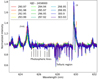 |
Fig. 1. Portion of all the normalized spectra. Each color stands for one observation. The same color code is used in all figures. |
2.3. Least-squares deconvolution
One convenient way to look at these data is to compute their least-squares deconvolution (LSD) profiles in both Stokes I and Stokes V spectra (Donati et al. 1997): The photospheric absorption lines and their Stokes V counterpart are weighted by their central wavelength, depth, and Landé factor; then these weighted lines are averaged altogether over one observation. We built a mask that identifies the lines to include in this computation using the VALD database4 (Piskunov et al. 1995; Ryabchikova et al. 2015). By scanning the average spectrum overplotted on a synthetic spectrum produced with the MARCS stellar atmosphere model (Gustafsson et al. 2008), we searched for undisturbed photospheric lines to be included. We did not include absorption lines that were contaminated by emission or telluric lines. Usually, the LSD I profiles we obtained exhibit distortions that are attributable to spots located at the photosphere level. In the case of LSD V, these profiles are shaped by the magnetic field along the line of sight at the surface of the star. The weak-field approximation assumes that the broadening of the photospheric profiles due to the Zeeman effect (proportional to the local magnetic intensity, along with the Landé factor and the central wavelength of a line) is negligible compared to all the other sources of broadening (instrumental broadening, thermal Doppler broadening, nonthermal Doppler broadening, and microturbulent and macroturbulent velocity dispersions). Combined in quadratic sum, these effects correspond to a broadening of Δvtot = 16.58 km s−1. For the specific case of S CrA N observed with ESPaDOnS, this Δvtot translates into B ≪ 10 kG. In other words, the use of the LSD profiles is justified when the surface averaged magnetic field does not reach or exceed 10 kG.
After applying the LSD computation with a Landé factor of 1.2 and a central wavelength of 500 nm to the complete Stokes I and V spectra, we obtained 12 sets of LSD I, LSD V, and LSD N profiles (Fig. 2). One profile represents one observation date, which is referred to as (HJD – 2458000) hereafter (see Table 1), for convenience. We report that the LSD N profiles show no spurious signal at any velocity for any observation.
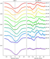 |
Fig. 2. LSD I and V profiles of S CrA N sorted by HJD (HJD–2458000 listed to the right of each plot) normalized by the maximum EW, observed at date 303.93. The color-coding is the same as in Fig. 1. The spacing between two profiles stands for the time span between the observations. Each profile is represented with a solid colored line and is surrounded by its uncertainties in faded color. The dotted black lines represent the reference Voigt profile for the I profiles and the continuum for the V profiles. The dashed vertical lines represent the radial velocity of the star. The V profiles are magnified by a factor 5 for clarity. |
3. Results
In this section, we present the methods we used for the analysis of the set of data introduced above. We also present our results.
3.1. Fit of the Stokes I spectra
We used the ZEEMAN code (Landstreet 1988; Wade et al. 2001; Folsom et al. 2018) to derive the stellar parameters of S CrA N from the fitting of photospheric lines in our spectra. The ZEEMAN code solves the radiative transfer assuming local thermodynamic equilibrium (LTE) in a 1D stellar atmosphere. We used the MARCS stellar atmosphere model, and the theoretical properties of the photospheric lines were extracted from the VALD database, as mentioned in Sect. 2.3. Then, the procedure for ZEEMAN is to adjust a synthetic spectrum to an observed spectrum by minimizing a χ2 function taking its seven free parameters into account. These parameters are the effective temperature Teff, the equatorial rotation velocity of the star projected on the line of sight v sin i, the radial velocity vr, the local veiling r, taken to be an excess continuum flux as a fraction of continuum, the surface gravity log g, the microturbulent velocity vmic, and the macroturbulent velocity vmac. A 7D χ2 map is likely to display several local minima. We therefore adjusted the parameters by pairs: Teff along with r, then v sin i along with vr, then vmic along with vmac, and log g was adjusted on its own. At first, all constant parameters were set to an arbitrary value until a minimum χ2 was reached for a considered pair of parameters. Then, the two previously fit quantities were set constant to their new value before we fitt two new parameters until we reached a new minimum χ2, which gives two different constant values to the new couple of parameters. This was repeated until all parameters were fit. Then, the procedure is repeated until a whole cycle of fitting produces no variation in any of the parameters. We tested the sensitivity to initial conditions by setting different starting values for each parameter, but the procedure always converged to the same set of values, except for log g and vmic. Their values did not change, regardless of the number of cycles performed, which shows little sensitivity of our fit to these parameters. For the procedure to run, we fixed log g = 4.0, which is common for CTTS, and derived the mass and radius as described in Sect. 4. Concerning vmic, we retained a value of 1 km s−1 that minimizes the χ2 function for the procedure to run, but did not derive any uncertainties based on the χ2 function. This fitting was made over 15 spectral windows (the central wavelengths of which are mentioned in Fig. 3) that display clear photospheric lines (i.e., deeper than 10% of the continuum level).
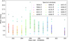 |
Fig. 3. Evolution of the average optical veiling with time. For each date, each color point stands for the mean veiling over one spectral window, whose center value is indicated in the caption. The error bars are centered on the average of the values computed over the 15 spectral windows and spread over their standard deviation. |
All our results are gathered in the first four rows of Table 2. Each value corresponds to the average of the values over the 15 spectral windows, and the uncertainty corresponds to their standard deviation. We obtained an effective temperature of Teff = 4300 ± 100 K. We retrieved a rotational velocity of v sin i = 10 ± 2 km s−1, where i = 0° corresponds to a face-on object. We obtained a radial velocity of vr = 0 ± 1 km s−1, and a macroscopic turbulence velocity vmac = 11 ± 3 km s−1. When we plot the veiling values against the spectral windows in which they were measured, no clear trend is observed, unlike in most CTTSs, where veiling decreases with wavelength in the optical domain (see, e.g., Fischer et al. 2011). When the veiling is plotted as a function of time for different spectral windows (Fig. 3), no clear periodicity can be identified, suggesting that an additional source must be at play in addition to the continuum emission from an accretion spot (e.g., accretion-powered emission lines). The mean veiling r over the 15 spectral windows and over time reaches 7 on average, and ranges between 4 and 11.
Stellar parameters of S CrA N.
3.2. Variability in LSD profiles
The LSD I profiles presented in Fig. 2 vary strongly in intensity, which is expected because of the changes in the veiling intensity. We found a negative correlation between the mean veiling and the equivalent width (EW) of the LSD I profile at each date. Thus, both LSD I and V profiles were scaled to the greatest EW (occurring at the Julian date 2 458 303.93) so that they all had the same EW. By doing so, we retained only their intrinsic shape variability, which presumably is due to spots.
The shape of the LSD I profiles changes entirely from one date to the next (Fig. 2). From date 291.98 to 292.95, for instance, the minimum intensity switches from the red to the blue side of the profile, and the low excess observed in the blue wing at first becomes reddened at 292.95. At date 303.93, the profile looks just like the profile at 291.98 again, with only minor changes in intensity. To try and constrain the origin of this variability, we checked whether the LSD I profiles were deformed differently, depending on the intrinsic depth of the lines included in the LSD mask (see Appendix B for the detailed procedure). Regardless of the depth limit of the lines taken into account for the LSD computation, the shapes of the profiles remain the same, with just a loss in signal-to-noise ratio (S/N) when removing more lines. We could not find a way to compute LSD I profiles with attenuated perturbations, and therefore, we adopted the LSD mask that gives the best S/N in the line profiles.
The source of these distortions must break the spherical symmetry of the surface of the star. Considering the high variability of our LSD I profiles, we cannot interpret them as deviations from a rest profile. Hence, we compared the LSD I profiles to a synthetic Voigt profile. We adjusted this profile by fitting it to the median LSD I observed within a velocity range of [−25 km s−1; +25 km s−1]. This reference profile is shown as a dotted line over the LSD I profiles in Fig. 2.
The V profiles also exhibit a variety of shapes, from flat (date 303.93) to typically antisymmetric (e.g., at date 292.95). We also note that similar I profiles can display very different V profiles. This is the case for the profiles at dates 293.99 and 303.93, where the I profiles are very similar, but the V profiles are strong and flat, respectively. Conversely, at dates 291.98, 292.95, and 293.99, the V profiles remain constant in intensity over the three observations, with just a smooth drift of the centroid from negative to positive velocities. In contrast, the I profiles are drastically different. There is no evident correlation between the I and V variations, suggesting that brightness inhomogeneities at the surface of S CrA N might have sources in addition to the brightness spots induced by the magnetic activity.
To recover the stellar rotation period, we computed 2D periodograms for the LSD I and V profiles (Fig. 4). We ran a Lomb-Scargle periodogram routine over each velocity channel (i.e., wavelength) to build the periodograms, where a time series of 12 unevenly sampled observations was considered. We restrained the search for periods longer than two days (Shannon theorem applied to a one-day sampling, which is the smallest sampling of our data) and shorter than 14 days. Any periodicity above or near 14 days cannot be considered reliable because that was the total span of our observations. False-alarm probability (FAP) contours of 3% are drawn in Fig. 4. All the FAPs of this study were computed assuming white noise in the continuum, that is, independent measurements, following the method described in Zechmeister & Kürster (2009). The 2D periodograms reveal no apparent periodicity in the LSD I profiles. While these profiles might be influenced by stochastic activity in the postshock region (see, e.g., Petrov et al. 2011; Dodin & Lamzin 2012; Rei et al. 2018), which could explain the deformations observed and might hide periodic features from hot/cool surface spots, the LSD V profiles are more robust to this contamination because the intensity of the magnetic field decreases rapidly with distance to the stellar surface (∝r−3 at least for a pure dipole). While the LSD I profiles display no clear periodicity, we can compute the 2D periodogram powers weighted by a 1-FAP factor over a range of velocity narrowed to the region of variability of the profiles (i.e., [−20 km s−1; +20 km s−1]) for each line of the LSD V periodogram. We are left with a 1D weighted periodogram whose peak maximum is the stellar rotation period and whose standard deviation is the uncertainty. This yields a period of 7.6 ± 1.3 days located at the extrema of the V profile, where the amplitude variation is strongest and strengthens the reliability of this signal detection.
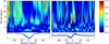 |
Fig. 4. 2D periodograms for the LSD I (left) and V (right) profiles. The dashed lines correspond to a period of 7.6 days (red) and an FAP = 3% contours (black). The average profiles (black line) surrounded by their 1σ deviations (light blue) are shown below the periodograms. |
3.3. Variability in emission lines
The CTTS are known to show strong and broad Balmer emission lines as well as a narrow emission in He I lines. They are all often associated with redshifted absorption features, indicating infall of material (Edwards et al. 1994; Beristain et al. 2001). It is now well accepted that a good part of these lines is formed through magnetospheric accretion (Hartmann et al. 1994, 2016). In our spectra, the Balmer and He I lines show various features both in emission and absorption, as well as strong variability. We therefore report below our analysis of this variability to understand the origin of the formation of these lines, and how they can constrain the magnetospheric accretion processes in a strongly accreting T Tauri star such as S CrA N.
3.3.1. Helium I λ5876
This line can be composite with up to three distinct components, which are particularly discernible in the case of S CrA N (Fig. 5 top).
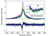 |
Fig. 5. He I λ5876 line for all observations. Stokes I (top) is normalized in intensity with respect to the continuum. Stokes V (bottom) is magnified by a factor of 5 for clarity. The color code is the same as in Fig. 2. The solid black lines are the average spectra. The dashed black lines represent the continuum level for each component. The dotted black line is the radial velocity of the star. The inset plot is a zoom on the absorption component. |
A narrow component (NC) that is asymmetric, extends from −30 km s−1 to 50 km s−1, and peaks around 0 km s−1. Due to its very high excitation potential, this emission line is thought to trace accretion footprints at the surface of the star.
A broad component (BC) that is ±250 km s−1 wide and is well reproduced by a Gaussian fit. Its origin is still poorly constrained, but it might itself be composite.
An absorption component (AC) in the red wing of the broad component (between ∼200 and ∼350 km s−1).
Strong Zeeman signatures are present in the Stokes V spectra (Fig. 5-bottom). The S-shaped signature spreads from −30 km s−1 to +50 km s−1 on average and is as strong as 20% of the continuum intensity. Due to its broadening and asymmetric shape, this V signal is attributed to the NC and thus traces the magnetic field at the footprint of the accretion columns. In order to study all the components separately, a fit with three independent Gaussian profiles was applied to each observed I profile. Each component was extracted by removing the models of the two other components from the profiles: the BC and AC Gaussian models were subtracted from the whole line because they matched the shape and intensity of the observed BC and AC at all phases. In contrast, removing its Gaussian model left significant NC residuals in the extracted BC and AC profiles due to the intrinsic asymmetry of the NC. Instead, a smoothed NC was subtracted from the original total profile, along with the AC/BC Gaussian model. This smoothed NC was obtained using a three-point moving average of the extracted NC.
We performed radial velocity, EW, and longitudinal field measurements in the NC. The longitudinal field was obtained with the first-moment method (Donati et al. 1997; Wade et al. 2000) The EW was computed between −30 km s−1 and +50 km s−1. Finally, we measured the radial velocity of the NC centroid by computing the first moment of the profile at each date. All three quantities are presented in Table 3 and Fig. 6. The radial velocity modulation was used to estimate the stellar period with a point-like accretion spot model described in further detail in Pouilly et al. (2021). We obtained a period P = 7.3 ± 0.2 days.
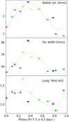 |
Fig. 6. Radial velocities (top), EW (middle), and longitudinal magnetic field (bottom) of the He I NC as a function of the stellar phase when considering a stellar rotation period of 7.3 ± 0.2 days and considering the first date of observation as ϕ = 0. When they are not visible, the uncertainties are smaller than the symbol. The dotted black lines illustrate the best fits we obtained, with a simple sine (middle and bottom) and the model of Pouilly et al. (2021; top). The color code is the same as in Fig. 1. |
Radial velocities, EW, and longitudinal field derived for each phase in the He I NC.
The 2D periodograms were computed for the V profiles and all three Stokes I components (Fig. 7). Each emitting component displays its own periodicity. The center of the NC shows a 7.4 ± 1.4-day period with a strong significance (FAP < 3%). However, this period drifts down to 6.6 ± 1.3 days in the red wing (above +30 km s−1). The BC shows a 3.2 ± 0.3-day period with a much lower significance (FAP ∼15%), but no signal at 7.4 days. The high power signal at long periods cannot be considered significant because it could not be observed for a full cycle, and the white-noise assumption in the FAP computations tends to overestimate its significance level. The AC displays a 6.6 ± 1.3-day period from 0 to +200 km s−1 and a 3.4 ± 0.4-day period beyond +200 km s−1. Both periods are detected with a high significance level (FAP < 3%). All the derived periods are gathered and compared in Fig. 8, and they are discussed in Sect. 4.
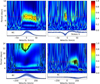 |
Fig. 7. 2D periodograms of the Stokes I NC (upper left), BC (lower left), AC (lower right), and Stokes V (upper right) in He I λ5876. The dashed red lines mark a period of 7.4 days (NC and Stokes V), 3.2 days (BC and AC), and 6.6 days (AC). The dashed black contours denote a constant FAP of 3% (except for 15% for the BC). The average profiles (black line) surrounded by their 1σ deviations (light blue) are shown below the periodograms. |
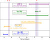 |
Fig. 8. Comparison of all the periods derived in this study, gathered according to the profile from which they arose. The dashed vertical red lines illustrate the stellar rotation period (P*) and half its value, surrounded by their uncertainty (light blue shade). All values are estimated from 2D periodograms except for (a), which is derived from radial velocities, and is chosen as P*. |
3.3.2. Balmer series
The detectable Balmer lines in the ESPaDOnS spectral range are displayed in Fig. 9. The corresponding periodograms exhibit signals at periods similar to those found in the LSD and helium profiles (see Appendix B). The regions of the lines associated with these periods are not the same for all the lines, however, making it hard to interpret which physical process causes their variability. General behaviors can still be retrieved. The emission lines are broad and asymmetric, ranging from −400 km s−1 to +400 km s−1 (even more for Hα). Albeit variable in intensity and shape, a persistent blueshifted absorption is present at all phases (peaking at about −100 km s−1). In addition to this absorption, a narrow emission can be observed in Hδ and Hγ, along with a redshifted absorption spreading from +50 to +300 km s−1. A similar redshifted absorption is barely detected in Hβ and cannot be seen in Hα, although its underlying presence could explain the asymmetry of the far wings in the latter. The exact span of this absorption is different for all the lines, however. The complexity of the Balmer lines can be interpreted as a multicomponent origin of the hydrogen emission, coming from different phenomena and/or different locations in the inner disk and magnetospheric regions, which we discuss in Sect. 4.
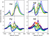 |
Fig. 9. Balmer series in S CrA N. The color code is the same as Fig. 2. The vertical dotted line shows the stellar radial velocity, and the horizontal dotted lines show the continuum level for each line. The y-scale of Hα has been changed for clarity. |
3.4. Correlations in spectral lines
We computed correlation matrices based on the Pearson coefficients to highlight different behaviors within a line profile and/or to link different lines between them (see, e.g., Kurosawa et al. 2005; Pouilly et al. 2020). More explicitly, for two given lines, we can compute the correlation between each pixel (i.e., velocity channel or wavelength) of the first line and each pixel of the second line based on the time series of these lines. For a pixel i in the first line and a pixel j in the second line, the correlation coefficient Rij between these pixels is given by
 (1)
(1)
with Cij the covariance between i and j,
 (2)
(2)
where N is the number of observations (12 here), Fi, k is the flux in pixel i for observation k, and  is the mean flux in pixel i over the N observations.
The coefficients of Rij hence range from −1 (perfect anticorrelation) to +1 (perfect correlation), with a null value meaning no correlation. To define some value above which we would consider a correlation level as significant, we computed one billion samples where two random variables were taken 12 times (one for each observation) in a white noise equivalent to our Stokes I RMS = 0.05. This gives a Gaussian distribution of Rij centered on 0 and with σ = 0.38. We chose to take a 2σ level of significance, corresponding to |Rij|≥0.76 for a significant correlation, while 0.38 ≤ |Rij|≤0.76 corresponds to a moderate correlation, and |Rij|≤0.38 corresponds to low correlation.
3.4.1. Correlations in He I
The decomposition of the helium line into BC and NC components is well justified by the autocorrelation matrix of the whole line (Fig. 10 top left). These components are neither correlated nor anticorrelated. Hence, their origin is linked to different processes. We searched for the correlations between each component and the Stokes V signature and found that the NC is well correlated with the positive peak of the V profile, but anticorrelated with the negative peak. The BC displays no clear correlation with any part of the V profile, confirming that the V signal is produced by the magnetic field in the formation region of the NC, and it is unrelated with the BC formation.
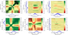 |
Fig. 10. Correlation matrices in He I (top row). Autocorrelation of the full helium line at 587.6 nm (left), correlation between the He I NC and the V profile (middle), and correlation between the He I BC and the V profile (right). Correlations matrices in Hα (bottom row). Autocorrelation of the full Hα line (left), correlation between the Hα line and the full He I line (middle), and correlation between the Hα line and the He I V profile (right). The dashed black contours show the 2σ significance level. The average profiles are represented at the bottom and left side of each panel (solid black line) and are surrounded by their standard deviation (light blue shade). The continuum level is shown with dashed black lines. |
3.4.2. Correlations in Hα
The bottom left panel in Fig. 10 shows the autocorrelation matrix of the Hα line. Two main components can be identified: a main broad symmetric emission (from −400 to 400 km s−1) that is truncated by a strong absorption from −200 to 0 km s−1. This blueshifted absorption is actually twofold: a saturated part spreads between −200 and −100 km s−1, and a variable part extends between −100 and 0 km s−1. This variable component is moderately anticorrelated (Rij < −0.38) with the broad emission.
3.4.3. Cross correlations between He I and Hα
All the correlations found between the Hα and the He I lines are moderate compared to those found for the previously mentioned autocorrelations matrices. Indications for a possible correlation are visible and presented here, however. The bottom middle panel of Fig. 10 shows that the He I NC seems correlated with the saturated part of the blueshifted absorption in the Hα line, even though the correlation coefficient does not reach the 2σ significance level. This partial correlation is confirmed in the bottom right panel of Fig. 10. The V profile exhibits the same correlation pattern, with both the variable part in the blueshifted absorption of Hα and the He I NC (see Fig. 10 top middle). A moderate anticorrelation (Rij ∼ −0.38) is found between the variable blueshifted absorption of Hα and the He I BC. However, considering the previous results, a negative correlation between the He I V profile and the He I BC was expected (Fig. 10 top right), which is not the case. Either there is no correlation between these components, or the underlying correlation is being quenched due to a potential crosstalk. A moderate correlation can also be found between the whole blueshifted absorption of Hα and the He I AC, with Rij ∼ 0.38 (light green area at the top of Fig. 10 bottom middle). This time, we do not have other diagnoses to confirm this correlation, however.
3.5. Magnetic field reconstruction
The Zeeman Doppler imaging (ZDI) technique uses the rotational modulation of Stokes V profiles to infer the large-scale magnetic configuration. We used the ZDIpy code, which assumes a decomposition of the field into spherical harmonics and adopts a weak-field approximation to reconstruct its topology, as described in full detail in Folsom et al. (2018). ZDIpy applies a regularized fitting algorithm that simultaneously maximizes the entropy of the reconstructed topology while keeping the corresponding χ2 below some target value (Skilling & Bryan 1984). The obtained map is therefore interpreted as the minimum information map fitting the observed LSD V data with a goodness determined by the target χ2.
The ZDI procedure described above usually also fits Stokes I profiles to reconstruct the brightness distribution of the star. However, for S CrA N, we never reached a satisfying fit for the LSD I and therefore assumed a uniform brightness. This uniform brightness was obtained with a Voigt model fitting the observed median shape of LSD I (see Fig. 2). In order to reconstruct the magnetic maps, the stellar rotation period and inclination with respect to the line of sight must be known. From the variability analysis of the He I line, we adopted a stellar period P* = 7.3 ± 0.2 days (see Table 2). Combining this stellar period with v sin i and the radius estimate presented in Sect. 4, we derive the stellar inclination i = 39° ±16°, which agrees at the 1σ level with the inclination of the inner disk as determined by GRAVITY Collaboration (2021; 27° ±3°). Considering the propagation of uncertainties in the computation of our stellar inclination, we adopt hereafter the value from GRAVITY Collaboration (2021) as the inclination of the star: i = 27° ±3°. The ZDI procedure ran over 16 iterations to maximize entropy, reaching the target-reduced χ2 of 1.5. This value represents the smallest target we could reach without fitting the noise of the data. The spherical harmonics expansion was truncated to consider only the modes where l ≤ 10 and reproduced the LSD V profiles between −25 km s−1 and +25 km s−1.
The reconstructed V profiles are overplotted on the observed LSD V profiles along with the derived magnetic maps in Fig. 11. The three maps represent the projection of the magnetic vector on the spherical basis, which translates into a radial field (positive polarity meaning a vector going out of the surface), azimuthal field (positive polarity meaning a vector oriented clockwise), and meridional field (positive polarity meaning a vector oriented toward the south). We represent on each map the rotation phases at which each observation is obtained, with the initial phase ϕ = 0 corresponding to the first observation date. The large-scale magnetic field that best reproduces our Stokes V profiles is as strong as 5.4 kG (which is within the weak-field approximation validity domain), with a mean intensity of 950 G, and a global axisymmetry of 68%. The poloidal component of this field (82% of the total energy) is primarily located in the dipolar component, which represents 27% of the total magnetic energy, even though higher-order poloidal modes are significantly present (up to 25% and 16% of the total magnetic energy for the quadrupole and the octupole, respectively). The maximum intensity (816 G) of this dipole is reached at an intermediate latitude (56°) at phase 0.29. The main magnetic properties of the system are listed in Table 4.
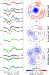 |
Fig. 11. Polar projection of the magnetic maps (right) reconstructed from the LSD V observations (left, colored lines). The black crosses overplotted on the LSD profiles show the reconstructed V, to the right of which the cycle number and phase are indicated. The red ticks surrounding each map show the observed phases clockwise, starting from the south. The dashed black circles show colatitudes of 27° (i), 63° (90−i) and 117° (90+i). The solid black line shows the equator. |
Main magnetic field properties from ZDI.
4. Discussion
4.1. S CrA N: A strong accretor?
Typical CTTS have effective temperatures between 3000 and 5000 K (spectral type G or later), masses most generally between 0.3 and 1 M⊙, with an upper limit of about 2 M⊙, and mass accretion rates of about 10−7 − 10−10 M⊙ yr−1. They probe the end of the fully convective Hayashi phase of the pre-main-sequence evolution, around ages of 1 to 2 Myr (e.g., Herczeg & Hillenbrand 2014; Villebrun et al. 2019; Nicholson et al. 2021).
When fitting our ESPaDOnS spectra, we found an effective temperature for S CrA N of 4300 ± 100 K, which agrees with the previous determinations (Table 2). We used the Gaia DR3 data and applied the method of Galli et al. (2020) to derive the distance to S CrA N (see Appendix C). We adopted a value of d = 152.4 ± 0.4 pc. We used the luminosity L* = 1.67 ± 0.8 L⊙ from Prato et al. (2003), corrected with our new distance to place S CrA N in the Hertzsprung-Russell diagram. Using the CESAM evolutionary model (Morel & Lebreton 2008; Marques et al. 2013), we estimated a mass M* = 0.8 ± 0.1 M⊙ and stellar radius R* = 2.3 ± 0.6 R⊙, which gives log g = 3.6 ± 0.2. The star is placed at an age of about 1 Myr, that is, it is younger than typical CTTSs. Like most of the CTTSs, S CrA N is then fully convective.
The photospheric lines of CTTSs generally appear to be shallower than those of nonaccreting stars, suggesting an excess of continuum emission. This so-called veiling can be observed in different regions of the spectrum of CTTSs, with different interpretations: in the near-infrared range, this excess might be attributed to the dust emission of the protoplanetary disk (Sousa et al. 2023), and in the ultraviolet-visible range, this excess is attributed to an accretion shock that behaves like a ∼8000 K blackbody continuum emission that is superimposed on the photospheric continuum. In very active stars, emission line spectra may also blend the photospheric lines, as early discussed in Bertout (1984), for example, and as shown in Petrov et al. (2011), Dodin & Lamzin (2012), and Rei et al. (2018), for instance. This veiling of optical spectral lines is typically lower than 2 around 5500 Å (Basri & Batalha 1990; Hartigan et al. 1991). In S CrA N, we found no trend between wavelength and the veiling, which is strongly variable around 5500 Å, with values ranging from 2 to 11. This finding is consistent with that of Sullivan et al. (2019), who also detected a strong variability and a large amplitude (between 2–6) of the veiling in the near-infrared range. Combined with its young age, this evidence of very strong accretion could indicate an evolutionary stage between Class I and Class II for S CrA N. This is further confirmed by the place of the S CrA system in the color-color diagram proposed by Koenig & Leisawitz (2014). With All-WISE measurements W1 = 5.1 ± 0.1, W2 = 4.0 ± 0.1, and W3 = 2.08 ± 0.01, the binary system is located at the frontier between protostars and T Tauri stars5.
4.2. Magnetosphere
From its fundamental parameters, S CrA N can be pictured as a young, fully convective T Tauri star. If the surface magnetic field of CTTSs were controlled by their internal structure alone, we might expect a strong (∼1 kG) axisymmetric large-scale field, mostly poloidal, with a strong dipole relative to higher poloidal modes (Gregory et al. 2012). This expectation is only partially met by the magnetic maps obtained in Sect. 3: the total field is mostly (82%) a poloidal field that is axisymmetric (73%), with a strong (816 G) dipole. However, the dipole and the quadrupole represent a similar portion of the poloidal field (33% and 30%, respectively), while the contribution from the octupole is lower, but still significant (19%). Our uncertainties on the luminosity may be the reason for this difference between the prediction and the reconstructed maps, but it should be noted that this region of the H-R diagram is observationally found to be populated with a variety of magnetic topologies (Donati et al. 2020; Nicholson et al. 2021). We also recall that S CrA N is a strong accretor, and that the possible impact of accretion on the inner structure of stars is yet to be explored.
We estimate the truncation radius (i.e., the radius at which the magnetic pressure equals the ram gas pressure) from this magnetic reconstruction, using the formula from Bessolaz et al. (2008),
 (3)
(3)
where the stellar field in the equatorial plane B* (i.e., half the dipole maximum intensity) was normalized to 140 G, the accretion rate ̇M to 10−8 M⊙ yr−1, the stellar mass to 0.8 M⊙, and the stellar radius to 2 R⊙, and where a Mach number of ∼1 was assumed. Because the ESPaDOnS data are not flux calibrated, we estimated the accretion rate based on the width of Hα at 10% of the peak intensity using the relation from Natta et al. (2004),
 (4)
(4)
where Hα10% is the considered width in km s−1, and ̇Macc is in M⊙ yr−1. With widths ranging from 579 km s−1 to 693 km s−1, we obtained accretion rate logarithms between −7.3 and −6.2 with a median value loġMacc = − 6.9 ± 0.7, which is consistent with the value of (1.0 ± 0.1)×10−7 M⊙ yr−1 from Sullivan et al. (2019) when correcting for the distance. Because they used the Brγ line to derive this accretion rate, we considered this value to be more reliable than our own (see Alcalá et al. 2014) for computing the truncation radius. Combined with the stellar radius and mass, and the magnetic topology from the present work, we obtained
 (5)
(5)
where the uncertainty was derived from the propagation of errors on the involved parameters through Eq. (3). This value is likely a lower boundary for the truncation radius because the ZDI technique is blind to the magnetic field in the region of formation of the emission lines, leading to an inconsistency between our reconstructed maps and the direct diagnoses of accretion, as shown below.
The derived truncation radius implies a colatitude of the accretion spot of 44° ±5° in a purely dipolar accretion model, which is consistent with the derived obliquity of the dipole from ZDI (56°). However, both values seem to contradict the very high apparent latitude of the postshock region as traced by the He I NC radial velocity curve (Fig. 6 top). The single-spot model from Pouilly et al. (2021) applied to these data gives a latitude of 86° ±1°. The asymmetry of the NC attributed to a velocity gradient in the postshock region does not vary with phase, which also supports the hypothesis that a spot is located at high latitude.
The magnetic field projected along the line of sight (or the longitudinal magnetic field Bl) associated with the NC of He I is positive at all phases (see Fig. 6 bottom, Table 3). If the NC arises from the postshock region, this means that at least part of the total magnetic field should be positive near the pole of the star, as shown earlier. However, the magnetic maps reconstructed from ZDI (Fig. 11) show that regions with a positive magnetic field (i.e., approaching the observer) in virtually every phase are only present in colatitudes higher than ∼60°, which corresponds to a portion of the star that is only occasionally visible (outside the second dashed black ring). This discrepancy leads us to consider the tomographic reconstructions presented in this work as not definite. Additional developments considering this emission line or any other line constraining a different region than the LSD profiles (e.g., the Ca II infrared triplet (IRT) or the Fe II 42 multiplet) are required to combine the different constraints into a single tomographic reconstruction (e.g., Donati et al. 2020), which is beyond the scope of this paper.
Finally, from this truncation radius, we can also deduce the expected accretion velocity vacc (i.e., the velocity of the gas free-falling from the truncation radius onto the stellar surface) based on energy conservation. This gas produces the AC observed in He I (Fig. 5), the higher members of the Balmer series (Fig. 9), and FeII (Fig. B.1). Based on our estimate of stellar mass and radius, we obtain vacc = 267 km s−1. This velocity is included in the range of velocities of the AC, which means that the value of Rt derived from ZDI is consistent with our values of M* and R*. However, the maximum velocity of the AC is higher than the free-fall velocity from infinity (v∞ = 370 km s−1), which either indicates an incorrect estimate of M* and R* or a significant broadening of these absorptions, the source of which remains unknown.
4.3. An unstable accretion regime?
The observed intensity and variability of various emission lines (e.g., He I, Fe II, and Ca II; see Appendix B) combined with the highly veiled photospheric lines suggest that intense accretion processes occur in the vicinity of S CrA N. One way to better constrain the accretion process is to compare the corotation radius and the truncation radius. When the ratio of truncation to corotation radius becomes low enough, Rayleigh-Taylor instability can be triggered at the magnetosphere-disk boundary (Kulkarni & Romanova 2008). Then, magnetospheric accretion enters the so-called unstable accretion regime, in which classical accretion funnels are observed, but accretion tongues as well. This phenomenon and its observable signatures have been extensively modeled (Kurosawa & Romanova 2013; Blinova et al. 2016) and have recently been reproduced in laboratory experiments that scale to the expected YSO accretion tongues (Burdonov et al. 2022). Blinova et al. (2016) observed unstable accretion for simulations where Rt/Rco < 0.71 for obliquities lower than 20°.
With the set of stellar parameters we derived (see Table 2), we computed a corotation radius of Rco = 6.4 ± 1.7 R*, which yields a ratio of truncation to corotation radius Rt/Rco = 0.33 ± 0.11, and places S CrA N in the unstable accretion scenario. The simulations from Kurosawa & Romanova (2013) showed that a proxy to the accretion regime lies in the profiles of the higher members of the Balmer series (Hγ and Hδ): in the stable case, redshifted absorption appears for about half the rotation cycle before it disappears, coming and going with stellar periodicity. This absorption is due to the visible accretion funnel that absorbs the stellar continuum while it remains in the line of sight. In the unstable case, this redshifted absorption is expected to be present at virtually every phase of the rotation cycle because there is at least one accretion tongue in the line of sight at all times. The profiles of Hγ and Hδ we observe in S CrA N display this absorption at all phases, as seen in Fig. 9, in agreement with unstable accretion.
4.4. Accreting structures
This unstable accretion regime sets a new context for the interpretation of the features observed in the emission lines presented earlier. The He I λ5876 NC likely arises from a postshock region in a single accretion spot located at high latitudes (∼86°). The origin in a postshock region is suggested by the low radial velocity of the flow producing the NC (∼2 km s−1; see Sect. 4.2). The single-spot model is corroborated by the consistency between the periodicity of the Stokes V signatures (both in the LSD profiles and the He I line) and the periodicity of the He I NC profiles. The longitudinal field curve in the He I line displays a complex modulation, with a substantial departure from the sine model near the extreme radial velocities, around phases 0.3 and 0.9 (see Fig. 6). This might be explained by a complex magnetic field of the star that differs significantly from a simple dipole, as suggested by ZDI from the present work. Finally, the asymmetry of the NC in Stokes I (steep blue wing and mild red wing; see Fig. 5) and the departure from antisymmetry in Stokes V (blue lobe stronger than red lobe) would come from the velocity gradient in the emission region. This asymmetry is observed at all phases without noticeable modulation, suggesting a high latitude for the accretion spot.
We speculate that the redshifted AC seen in He I λ5876, Hγ, and Hδ is formed in two distinct structures: first, in an accretion funnel located around phase 0.2 (called the “main” column hereafter), which produces the NC at its footprint when it forms an accretion shock; then, in another accretion column located around phase 0.7 (called the “secondary” column hereafter, in contrast to the main column), which lacks an NC counterpart, because its density is much lower than in the main column, where accretion is favored by the magnetic misalignment. An AC is nonetheless produced by the free-falling material of the secondary column, which absorbs the light emerging from the photosphere. These opposite structures then produce an artificial periodicity of half the stellar period (P*/2 = 3.65 ≃ 3.4 ± 0.4 days; see Fig. 8), the actual stellar period being detected for the lowest velocities of the AC (P* = 7.3 ≃ 6.6 ± 1.3 days), because only the main accretion column is dense enough at low velocities (i.e., in the upper part of the column) to produce an absorption.
Finally, the He I λ5876 BC is most likely formed by the in-falling gas in both the main and the secondary funnels because the same artificial periodicity is observed as in the AC, and its centroid is mostly redshifted. As discussed in Beristain et al. (2001), this tendency in the central velocity of the line can be obtained with material that follows a purely dipolar field at polar angles lower than 54.7°, which corresponds to accreting gas.
4.5. Outflows
Lima et al. (2010) modeled the Hα line in the case of a CTTS undergoing both magnetospheric accretion and a disk wind. When we compare the Hα lines we observed (Fig. 9) with their grids of models, the deep blueshifted absorption of our profiles appears to be well reproduced with their models combining a high accretion rate (10−7 M⊙ yr−1) and a hot (∼8000 − 10 000 K) disk wind with a density of a few 10−11 g cm−3 and an outer radius of a few dozen stellar radii (see their Figs. 4 and 6). Their model reproduces the bulk of the absorption, but not the variable features seen at low velocities. We guess that these features stem from disk outflows because they are moderately correlated with accretion signatures (i.e., the He I NC and He I AC), as shown in Fig. 10. Numerical simulations (Romanova et al. 2009; Zanni & Ferreira 2013; Pantolmos et al. 2020) have shown that the stellar magnetic field lines threading the disk outside the accretion columns are open, further producing transient ejections (i.e., magnetospheric ejections/conical winds) and/or disk winds. These outflows are also suspected when we compare the truncation radius we computed with the size of the region emitting the hydrogen Brγ line in S CrA N. This region can be spatially constrained to RBrγ = 7.7 ± 2.2 R* through interferometric observations (GRAVITY Collaboration 2017b, 2023). The given value is an update from GRAVITY Collaboration (2023) with our new values for the distance and R*. Because RBrγ extends well beyond Rt = 2.1 ± 0.4 R*, disk outflows must account for part of the emission observed in this line.
Finally, the Herbig-Haro object HH729 has been attributed to S CrA N (Peterson et al. 2011). The forbidden lines of [OI] at 6300.2 Å and 6363.8 Å and [SII] at 6730 Å are usually interpreted as tracers of outflows at different scales (see, e.g., Alexander et al. 2014; Pascucci et al. 2020; Gangi et al. 2023). These lines are present in the spectra of S CrA N with a strong blueshifted peak (∼ − 120 km s−1) and an asymmetry (see Appendix B for the profiles), strengthening the idea that a large-scale outflow arises from the inner regions.
5. Conclusions
Based on spectropolarimetric observations in the optical range with ESPaDOnS at CFHT, we have probed the star-disk interaction in the innermost regions of the northern component of the young binary system S CrA. With its confirmed high accretion rate (10−7 M⊙ yr−1), this object is an ideal target for studying the magnetospheric accretion scenario in a stronger regime than in CTTSs. Our main findings are summarized below.
When we fit the ESPaDOnS spectra and using CESAM evolutionary models, S CrA N appears to have a mass of 0.8 M⊙, to be fully convective, and about 1 Myr old. As in previous determinations in the near-infrared range, the veiling we derive around 5500 Å is strongly variable and high (i.e., ranging from 2 to 11), which suggests that the star is located in a strong accretion regime. Combined with the young age, this could indicate an evolutionary stage between Class I and Class II.
This evolutionary stage is also in line with the large-scale magnetic field we reconstructed through ZDI. We obtained a total field as strong as 5.4 kG and not strongly axisymmetric, whose dipolar contribution represents about one-third of the total field. Higher poloidal orders being significant (∼50%), the large-scale topology of the magnetic field appears to be rather complex when compared with CTTSs.
Additional developments are needed for a complete and coherent view of the magnetic topology of S CrA N by including the constraints from the emission lines (e.g., He I and the Ca II IRT or the Fe II 42 multiplet) and developing more complex models to reproduce the emitting regions of these lines and their properties.
We derive a magnetic truncation radius of ∼2 R* and a corotation radius of ∼6 R*, suggesting that S CrA N is in an unstable accretion regime. Based on the helium and hydrogen line profiles and periodicities, we suggest that this accretion occurs in an unstable scenario, along two distinct accretion structures: one main accretion column associated with the accretion shock, and a secondary accretion column with much lower density in it that produces no detectable accretion shock.
The emission lines of the hydrogen Balmer series are highly variable and display multicomponent profiles. The observed Hα line profiles exhibit clear signatures of an outflow and agree well with simulations of a hot and dense disk wind. This finding is compatible with the size of the Brγ emitting region measured with GRAVITY (∼8 R*) which is substantially larger than the truncation radius.
Our spectropolarimetric campaign in the optical allows us to characterize the star-disk interactions in the innermost regions of S CrA N, and when combined with near-infrared interferometry, to provide a consistent view of these complex and variable regions. The strong and unstable accretion regime is strong and unstable, and therefore, probing the accretion-ejection processes would benefit from a temporal follow-up of these phenomena through simultaneous observations combining photometry, spectroscopy, and interferometry in various spectral ranges.
GRAVITY: general relativity analysis via vlti interferometer.
MIDI: mid-infrared interferometric instrument.
PIONIER: precision integrated-optics near-infrared imaging experiment.
VALD database: http://vald.astro.uu.se/
With All-WISE, S CrA N was observed together with S CrA S, due to the angular resolution of the observations (∼6″). Because the two components are coeval (Gahm et al. 2018), this does not affect the interpretation regarding their young age.
http://www.ast.obs-mip.fr/projets/espadons/espadons.html
S CrA N Gaia ID : 6731210253964165632
S CrA S Gaia ID : 6731210258265107584
Acknowledgments
This work is supported by the French National Research Agency in the framework of the “investissements d’avenir” program (ANR-15-IDEX-02). This project has received funding from the European Research Council (ERC) under the European Union’s Horizon 2020 research and innovation program (grant agreement no. 742095; SPIDI: Star-Planets-Inner Disk-Interactions, http://www.spidi-eu.org). This work has made use of data from the European Space Agency (ESA) mission Gaia (https://www.cosmos.esa.int/gaia), processed by the Gaia Data Processing and Analysis Consortium (DPAC, https://www.cosmos.esa.int/web/gaia/dpac/consortium). Funding for the DPAC has been provided by national institutions, in particular the institutions participating in the Gaia Multilateral Agreement. This work has made use of the VALD database, operated at Uppsala University, the Institute of Astronomy RAS in Moscow, and the University of Vienna. Finally, we address our greatest thanks to the referee of this article for their fruitful suggestions and comments.
References
- Alcalá, J. M., Natta, A., Manara, C. F., et al. 2014, A&A, 561, A2 [NASA ADS] [CrossRef] [EDP Sciences] [Google Scholar]
- Alcalá, J. M., Gangi, M., Biazzo, K., et al. 2021, A&A, 652, A72 [NASA ADS] [CrossRef] [EDP Sciences] [Google Scholar]
- Alencar, S. H. P., Bouvier, J., Walter, F. M., et al. 2012, A&A, 541, A116 [NASA ADS] [CrossRef] [EDP Sciences] [Google Scholar]
- Alencar, S. H. P., Bouvier, J., Donati, J. F., et al. 2018, A&A, 620, A195 [NASA ADS] [CrossRef] [EDP Sciences] [Google Scholar]
- Alexander, R., Pascucci, I., Andrews, S., Armitage, P., & Cieza, L. 2014, in Protostars and Planets VI, eds. H. Beuther, R. S. Klessen, C. P. Dullemond, & T. Henning, 475 [Google Scholar]
- Anthonioz, F., Ménard, F., Pinte, C., et al. 2015, A&A, 574, A41 [NASA ADS] [CrossRef] [EDP Sciences] [Google Scholar]
- Baraffe, I., Elbakyan, V. G., Vorobyov, E. I., & Chabrier, G. 2017, A&A, 597, A19 [NASA ADS] [CrossRef] [EDP Sciences] [Google Scholar]
- Basri, G., & Batalha, C. 1990, ApJ, 363, 654 [Google Scholar]
- Beristain, G., Edwards, S., & Kwan, J. 2001, ApJ, 551, 1037 [Google Scholar]
- Bertout, C. 1984, Rep. Prog. Phys., 47, 111 [NASA ADS] [CrossRef] [Google Scholar]
- Bessolaz, N., Zanni, C., Ferreira, J., Keppens, R., & Bouvier, J. 2008, A&A, 478, 155 [NASA ADS] [CrossRef] [EDP Sciences] [Google Scholar]
- Blinova, A. A., Romanova, M. M., & Lovelace, R. V. E. 2016, MNRAS, 459, 2354 [Google Scholar]
- Bouvier, J., Alencar, S. H. P., Harries, T. J., Johns-Krull, C. M., & Romanova, M. M. 2007, in Protostars and Planets V, eds. B. Reipurth, D. Jewitt, & K. Keil, 479 [Google Scholar]
- Bouvier, J., Perraut, K., Le Bouquin, J. B., et al. 2020, A&A, 636, A108 [NASA ADS] [CrossRef] [EDP Sciences] [Google Scholar]
- Burdonov, K., Yao, W., Sladkov, A., et al. 2022, A&A, 657, A112 [NASA ADS] [CrossRef] [EDP Sciences] [Google Scholar]
- Camenzind, M. 1990, Rev. Mod. Astron., 3, 234 [Google Scholar]
- Cazzoletti, P., Manara, C. F., Liu, H. B., et al. 2019, A&A, 626, A11 [NASA ADS] [CrossRef] [EDP Sciences] [Google Scholar]
- Dodin, A. V., & Lamzin, S. A. 2012, Astron. Lett., 38, 649 [Google Scholar]
- Donati, J. F. 2003, in Solar Polarization, eds. J. Trujillo-Bueno, & J. Sanchez Almeida, ASP Conf. Ser., 307, 41 [Google Scholar]
- Donati, J. F., Semel, M., Carter, B. D., Rees, D. E., & Collier Cameron, A. 1997, MNRAS, 291, 658 [Google Scholar]
- Donati, J. F., Bouvier, J., Alencar, S. H., et al. 2020, MNRAS, 491, 5660 [Google Scholar]
- Edwards, S. 1979, PASP, 91, 329 [NASA ADS] [CrossRef] [Google Scholar]
- Edwards, S., Hartigan, P., Ghandour, L., & Andrulis, C. 1994, AJ, 108, 1056 [Google Scholar]
- Espaillat, C. 2022, in AAS Meeting Abstracts, 54, 413.01 [NASA ADS] [Google Scholar]
- Fischer, W., Edwards, S., Hillenbrand, L., & Kwan, J. 2011, ApJ, 730, 73 [Google Scholar]
- Folsom, C. P., Bouvier, J., Petit, P., et al. 2018, MNRAS, 474, 4956 [NASA ADS] [CrossRef] [Google Scholar]
- Gahm, G. F., Petrov, P. P., Tambovsteva, L. V., et al. 2018, A&A, 614, A117 [NASA ADS] [CrossRef] [EDP Sciences] [Google Scholar]
- Gaia Collaboration (Vallenari, A., et al.) 2023, A&A, 674, A1 [NASA ADS] [CrossRef] [EDP Sciences] [Google Scholar]
- Galli, P. A. B., Bouy, H., Olivares, J., et al. 2020, A&A, 634, A98 [NASA ADS] [CrossRef] [EDP Sciences] [Google Scholar]
- Gangi, M., Nisini, B., Manara, C. F., et al. 2023, A&A, 675, A153 [NASA ADS] [CrossRef] [EDP Sciences] [Google Scholar]
- GRAVITY Collaboration (Abuter, R., et al.) 2017a, A&A, 602, A94 [NASA ADS] [CrossRef] [EDP Sciences] [Google Scholar]
- GRAVITY Collaboration (Garcia Lopez, R., et al.) 2017b, A&A, 608, A78 [NASA ADS] [CrossRef] [EDP Sciences] [Google Scholar]
- GRAVITY Collaboration (Garcia Lopez, R., et al.) 2020, Nature, 584, 547 [Google Scholar]
- GRAVITY Collaboration (Perraut, K., et al.) 2021, A&A, 655, A73 [NASA ADS] [CrossRef] [EDP Sciences] [Google Scholar]
- GRAVITY Collaboration (Wojtczak, J. A., et al.) 2023, A&A, 669, A59 [Google Scholar]
- Gregory, S. G., Donati, J. F., Morin, J., et al. 2012, ApJ, 755, 97 [Google Scholar]
- Gustafsson, B., Edvardsson, B., Eriksson, K., et al. 2008, A&A, 486, 951 [NASA ADS] [CrossRef] [EDP Sciences] [Google Scholar]
- Hartigan, P., Kenyon, S. J., Hartmann, L., et al. 1991, ApJ, 382, 617 [Google Scholar]
- Hartmann, L., Hewett, R., & Calvet, N. 1994, ApJ, 426, 669 [Google Scholar]
- Hartmann, L., Herczeg, G., & Calvet, N. 2016, ARA&A, 54, 135 [Google Scholar]
- Herczeg, G. J., & Hillenbrand, L. A. 2014, ApJ, 786, 97 [Google Scholar]
- Koenig, X. P., & Leisawitz, D. T. 2014, ApJ, 791, 131 [Google Scholar]
- Koenigl, A. 1991, ApJ, 370, L39 [Google Scholar]
- Kulkarni, A. K., & Romanova, M. M. 2008, MNRAS, 386, 673 [Google Scholar]
- Kurosawa, R., & Romanova, M. M. 2013, MNRAS, 431, 2673 [Google Scholar]
- Kurosawa, R., Harries, T. J., & Symington, N. H. 2005, MNRAS, 358, 671 [Google Scholar]
- Landstreet, J. D. 1988, ApJ, 326, 967 [Google Scholar]
- Lima, G. H. R. A., Alencar, S. H. P., Calvet, N., Hartmann, L., & Muzerolle, J. 2010, A&A, 522, A104 [NASA ADS] [CrossRef] [EDP Sciences] [Google Scholar]
- Manara, C. F., Frasca, A., Venuti, L., et al. 2021, A&A, 650, A196 [NASA ADS] [CrossRef] [EDP Sciences] [Google Scholar]
- Marques, J. P., Goupil, M. J., Lebreton, Y., et al. 2013, A&A, 549, A74 [NASA ADS] [CrossRef] [EDP Sciences] [Google Scholar]
- Marraco, H. G., & Rydgren, A. E. 1981, AJ, 86, 62 [CrossRef] [Google Scholar]
- Martin, A. J., Neiner, C., Oksala, M. E., et al. 2018, MNRAS, 475, 1521 [NASA ADS] [CrossRef] [Google Scholar]
- Morel, P., & Lebreton, Y. 2008, Ap&SS, 316, 61 [Google Scholar]
- Natta, A., Testi, L., Muzerolle, J., et al. 2004, A&A, 424, 603 [NASA ADS] [CrossRef] [EDP Sciences] [Google Scholar]
- Nicholson, B. A., Hussain, G., Donati, J. F., et al. 2021, MNRAS, 504, 2461 [NASA ADS] [CrossRef] [Google Scholar]
- Ortiz, J. L., Sugerman, B. E. K., de La Cueva, I., et al. 2010, A&A, 519, A7 [NASA ADS] [CrossRef] [EDP Sciences] [Google Scholar]
- Pantolmos, G., Zanni, C., & Bouvier, J. 2020, A&A, 643, A129 [NASA ADS] [CrossRef] [EDP Sciences] [Google Scholar]
- Pantolmos, G., Zanni, C., & Bouvier, J. 2022, in Cambridge Workshop on Cool Stars, Stellar Systems, and the Sun, 48 [Google Scholar]
- Pascucci, I., Banzatti, A., Gorti, U., et al. 2020, ApJ, 903, 78 [Google Scholar]
- Peterson, D. E., Caratti o Garatti, A., Bourke, T. L., et al. 2011, ApJS, 194, 43 [NASA ADS] [CrossRef] [Google Scholar]
- Petrov, P. P., Gahm, G. F., Stempels, H. C., Walter, F. M., & Artemenko, S. A. 2011, A&A, 535, A6 [NASA ADS] [CrossRef] [EDP Sciences] [Google Scholar]
- Piskunov, N. E., Kupka, F., Ryabchikova, T. A., Weiss, W. W., & Jeffery, C. S. 1995, A&AS, 112, 525 [Google Scholar]
- Pouilly, K., Bouvier, J., Alecian, E., et al. 2020, A&A, 642, A99 [NASA ADS] [CrossRef] [EDP Sciences] [Google Scholar]
- Pouilly, K., Bouvier, J., Alecian, E., et al. 2021, A&A, 656, A50 [NASA ADS] [CrossRef] [EDP Sciences] [Google Scholar]
- Prato, L., Greene, T. P., & Simon, M. 2003, ApJ, 584, 853 [Google Scholar]
- Rei, A. C. S., Petrov, P. P., & Gameiro, J. F. 2018, A&A, 610, A40 [NASA ADS] [CrossRef] [EDP Sciences] [Google Scholar]
- Reipurth, B., & Zinnecker, H. 1993, A&A, 278, 81 [NASA ADS] [Google Scholar]
- Romanova, M. M., Ustyugova, G. V., Koldoba, A. V., & Lovelace, R. V. E. 2009, MNRAS, 399, 1802 [Google Scholar]
- Ryabchikova, T., Piskunov, N., Kurucz, R. L., et al. 2015, Phys. Scr., 90 [Google Scholar]
- Rydgren, A. E. 1977, PASP, 89, 557 [NASA ADS] [CrossRef] [Google Scholar]
- Schegerer, A. A., Wolf, S., Hummel, C. A., Quanz, S. P., & Richichi, A. 2009, A&A, 502, 367 [NASA ADS] [CrossRef] [EDP Sciences] [Google Scholar]
- Skilling, J., & Bryan, R. K. 1984, MNRAS, 211, 111 [NASA ADS] [CrossRef] [Google Scholar]
- Sousa, A. P., Bouvier, J., Alencar, S. H. P., et al. 2021, A&A, 649, A68 [NASA ADS] [CrossRef] [EDP Sciences] [Google Scholar]
- Sousa, A. P., Bouvier, J., Alencar, S. H. P., et al. 2023, A&A, 670, A142 [NASA ADS] [CrossRef] [EDP Sciences] [Google Scholar]
- Sullivan, K., Prato, L., Edwards, S., Avilez, I., & Schaefer, G. H. 2019, ApJ, 884, 28 [NASA ADS] [CrossRef] [Google Scholar]
- Varga, J., Ábrahám, P., Chen, L., et al. 2018, A&A, 617, A83 [NASA ADS] [CrossRef] [EDP Sciences] [Google Scholar]
- Villebrun, F., Alecian, E., Hussain, G., et al. 2019, A&A, 622, A72 [NASA ADS] [CrossRef] [EDP Sciences] [Google Scholar]
- Wade, G. A., Donati, J. F., Landstreet, J. D., & Shorlin, S. L. S. 2000, MNRAS, 313, 851 [CrossRef] [Google Scholar]
- Wade, G. A., Bagnulo, S., Kochukhov, O., et al. 2001, A&A, 374, 265 [NASA ADS] [CrossRef] [EDP Sciences] [Google Scholar]
- Walker, M. F. 1972, ApJ, 175, 89 [NASA ADS] [CrossRef] [Google Scholar]
- Zanni, C., & Ferreira, J. 2013, A&A, 550, A99 [NASA ADS] [CrossRef] [EDP Sciences] [Google Scholar]
- Zechmeister, M., & Kürster, M. 2009, A&A, 496, 577 [CrossRef] [EDP Sciences] [Google Scholar]
Appendix A: Influence of the southern component
In order to address the possible contamination of our observations by S CrA S, we simulated the observed field of view (FoV) of ESPaDOnS. We placed S CrA S at a distance of 1.4" from S CrA N (astrometry from Gaia Collaboration 2023), and accounted for a circular FoV of 1.6" (from the official ESPaDOnS website6) centered on S CrA N. We attributed a normalized flux of 1 for S CrA N, hence a flux of 0.63 for S CrA S based on a difference in magnitude of 0.5 in the I band (Gahm et al. 2018). Finally, we applied a seeing as a 2D Gaussian distribution centered on each star, with its full width at half maximum equal to the seeing of our observations (see Table 1). This description represents the actual observation, and we computed the total flux observed as the sum of the flux in each pixel within the FoV. We also computed the sole contribution of S CrA S by modifying the model as such: the FoV was untouched in size and position, but we only took the Gaussian model of S CrA S into account (i.e., not fully included inside the FoV). The contribution of S CrA S is then the sum of the flux in each pixel within the FoV. The ratio of these fluxes gives the contribution of S CrA S to the total flux observed. This method yields a contribution of 8.96% at worst (seeing of 1350 mas), with a minimum of 0.03% (seeing of 430 mas) and an average of 1.58% (seeing = 750 mas). Three observations exceeded a contribution of 5%: the observations on June 26, 27, and 28, with 9.0%, 9.3%, and 5.3%, respectively. All the results obtained in this work were verified without these three observations. No significant difference was found, except for a decrease in S/N.
Appendix B: Spectra of S CrA N
B.1. Classical emission lines in classical T Tauri Stars
Some lines that typically trace the accretion-ejection processes in CTTSs are displayed in Figure B.1. We provide a short comment on the aspect and behavior for each of these lines.
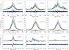 |
Fig. B.1. Emission lines in S CrA N. All V profiles, magnified by a factor 5 for clarity. The rainbow shading has the same meaning as in Figure 1, and the solid black line shows the median profile. |
B.1.1. Iron triplet
This triplet is thought to originate from the chromospheric activity of the star. It is presented in the top row of Fig. B.1. It is highly variable and strong. The lines exhibit two common features: A broad and a narrow emission, both centered near the radial velocity of the star. The lines at λ4924 and λ5018 also have an additional redshifted absorption at high velocities, which are likely to be interpreted just like those observed in He I λ5876, Hγ, and Hδ. Their Stokes V profiles show antisymmetric signatures associated with the narrow emissions, which are exceptionally strong and symmetric. Combined with the simple decomposition of their Stokes I counterparts, this makes them good candidates for a future tomographic reconstruction taking emission lines as constraints.
B.1.2. Calcium infrared triplet (IRT)
Commonly used to study the activity of CTTSs, this triplet is presented in the middle row of Fig. B.1. Its intensities are comparable to those of Hα, which places these lines among the most dominant lines in the spectrum of S CrA N. Their shape is complex, and no simple decomposition (based on the sum of up to four Gaussians) was successful in reproducing them. The Stokes V signatures are strong and define a narrow component that is emitted near the surface of the star, unlike the rest of the lines.
B.1.3. He Iλ6678
This line likely originates from the same processes as He I λ5876. Its different excitation potential is used to compute line ratios and infer the electron density and temperature encountered in the region producing these lines. No attempt to derive these parameters was tried in this work. The decomposition of this line appears to be similar to that of He I λ5876, except for the noticeable absence of the redshifted AC.
B.1.4. Oxygen
This forbidden line of oxygen is usually threefold (see, e.g., Pascucci et al. 2020): A narrow low-velocity component (NLVC) traces a wind arising in the outermost part of the inner disk (∼ 1 au). A broad low-velocity component (BLVC) traces a wind arising in the innermost part of the inner disk (≤ 0.1 au). A high-velocity blueshifted component (HVC) traces a jet. The HVC is observed to peak around -120 km/s and is confirmed by a Herbig Haro object (HH729) associated with S CrA N. In the low-velocity components, S CrA N seems to display a BLVC without an NLVC, which is unexpected because disk-evaporation models predict an evolution going from BLVC + NLVC (when the inner wind is dense enough to shield sthe outer disk from high-energy stellar photons) to NLVC as the inner wind density decreases and the disk starts to evaporate (Alexander et al. 2014). Because the disk is not expected to evaporate before the late Class II stage, another model should be invoked to explain the profiles observed in S CrA N (Class I - Class II transition stage). No Stokes V signal is detected, as expected from a line that formed away from the star, in a region in which the magnetic field is weak.
B.1.5. Sulfur
Just like for the forbidden oxygen line, this line traces a jet. The peak occurs at similar velocities as the HVC of OI: ∼ -120 km/s.
B.2. Variability of the Balmer series
The Balmer series are composite lines, as discussed in this work. Their 2D periodograms are shown in Fig. B.2. Multiple signals are visible, but as discussed in the main text, the longer periods are not commented on because of the white-noise assumption made in the computation of the periodograms, and because of the total span of observation, which does not allow us to observe these periodicities for more than a full cycle. The blue side of the broad emission (near -180 km/s) has a periodicty of about that of the stellar rotation period (7.3 ± 0.2 days) in all the lines but Hδ. The red side of this broad absorption (near +100 km/s) has no clear periodicity for Hα and Hβ, while a somewhat significant signal near 4 days is visible for Hγ and Hδ. This periodicity is not found in any other feature we studied in this work, and its origin remains unknown. The redshifted absorption seen in Hβ, Hγ, and Hδ, which was extensively discussed in previous sections, is found to be periodic with a period similar to that in the redshifted absorption met in the He I λ5876 line. That is, slightly lower than half the rotation period (3.2 days instead of 3.65 days)
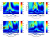 |
Fig. B.2. 2D periodograms of the lower Balmer series. The dashed red lines show periods of 7.3 days (P*) and 3.65 days (P*/2). The dashed black contour shows the 3% FAP level. |
B.3. LSD profile dependence on the line depth
In order to test the potential influence of the depth of the lines that were taken into account during the LSD procedure, we performed a test in which we excluded the deepest lines, which should be the most affected by veiling (Rei et al. 2018), and the lines located within their ± 15 km/s vicinity, which could be affected by them. We applied different depths thresholds to obtain a mask and computed the resulting LSD I and V profiles. We illustrate this with three different masks in Fig.B.3. The first mask is the one we cleansed naturally, that is, without any depth threshold (green curves). It includes 10 263 lines out of the 27,502 coming from the raw synthetic spectrum. Then, with a threshold of 0.8, only 7,301 lines were left in the mask (blue curve). Finally, with a threshold of 0.4, 4,279 lines remained (red curve). At this stage, the profile S/N becomes so low that any further cut would significantly impact the LSD signal. Fig. B.3 shows that regardless of the depth limit applied to a mask, the qualitative shape of the LSD profiles remains constant. We can then exclude continuum veiling as the source of the quick and intense variations observed in our LSD profiles, and we favor an origin in the chromospheric emission lines.
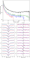 |
Fig. B.3. Illustration of the line depth test. Top: Number of lines included in each mask as a function of their intrinsic depth. Bottom left: LSD I profiles associated with each mask. Bottom right: LSD V profiles (magnified by a factor 5 for clarity) associated with each mask. The black curve stands for the raw synthetic spectrum. The green curve corresponds to the mask used in this study. The blue curve corresponds to a depth limit of 0.8. The red curve corresponds to a depth limit of 0.4. |
Appendix C: Distance estimate of the S CrA system
The distance found for S CrA N in the most recent literature comes from Prato et al. (2003) with 130 ± 20 pc. This value was taken from an even earlier estimate of the distance of the whole R CrA T region by Marraco & Rydgren (1981), while the associated uncertainty was simply assumed a priori and was not derived from the observations. The latest Gaia-DR3 data (Gaia Collaboration 2023) provide a distance of 160 ± 2 pc for S CrA N from its parallax measurements7, while S CrA S is found to be at 147 ± 2 pc with the same data release8, which is inconsistent with the assumption that S CrA is a close binary. This discrepancy alone is not enough to question the binarity of the S CrA system, however. The nebulosity in its surroundings, coupled with its binary nature, can explain this discrepancy in the Gaia parallax measurements. Galli et al. (2020) used the Gaia-DR2 data on a sample of 313 stars associated with the Corona Australis region to draw a line between the so-called on-cloud and off-cloud subregions. In their study, this distinction was based on a Bayesian distance estimate and on tangential velocities measurements. Using the Gaia-DR3 data, we placed S CrA S and S CrA N in the diagram in Figure C.1 (proper motion in right ascension against proper motion in declination for both Gaia DR2 and DR3 data) adapted from Galli et al. (2020) and unambiguously assigned S CrA N to the on-cloud region with a proper motion of 7.05 ± 0.06 mas/yr in right ascension and −26.51 ± 0.06 mas/yr in declination. We thus adopted the distance of the on-cloud region, that is, 152.4 ± 0.4 pc for S CrA N.
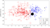 |
Fig. C.1. Proper motions for the two subgroups of the Corona Australis region in Gaia DR2, S CrA N and S CrA S in Gaia DR2 and Gaia DR3. Adapted from Galli et al. (2020). |
All Tables
Radial velocities, EW, and longitudinal field derived for each phase in the He I NC.
All Figures
|
Fig. 1. Portion of all the normalized spectra. Each color stands for one observation. The same color code is used in all figures. |
| In the text | |
|
Fig. 2. LSD I and V profiles of S CrA N sorted by HJD (HJD–2458000 listed to the right of each plot) normalized by the maximum EW, observed at date 303.93. The color-coding is the same as in Fig. 1. The spacing between two profiles stands for the time span between the observations. Each profile is represented with a solid colored line and is surrounded by its uncertainties in faded color. The dotted black lines represent the reference Voigt profile for the I profiles and the continuum for the V profiles. The dashed vertical lines represent the radial velocity of the star. The V profiles are magnified by a factor 5 for clarity. |
| In the text | |
|
Fig. 3. Evolution of the average optical veiling with time. For each date, each color point stands for the mean veiling over one spectral window, whose center value is indicated in the caption. The error bars are centered on the average of the values computed over the 15 spectral windows and spread over their standard deviation. |
| In the text | |
|
Fig. 4. 2D periodograms for the LSD I (left) and V (right) profiles. The dashed lines correspond to a period of 7.6 days (red) and an FAP = 3% contours (black). The average profiles (black line) surrounded by their 1σ deviations (light blue) are shown below the periodograms. |
| In the text | |
|
Fig. 5. He I λ5876 line for all observations. Stokes I (top) is normalized in intensity with respect to the continuum. Stokes V (bottom) is magnified by a factor of 5 for clarity. The color code is the same as in Fig. 2. The solid black lines are the average spectra. The dashed black lines represent the continuum level for each component. The dotted black line is the radial velocity of the star. The inset plot is a zoom on the absorption component. |
| In the text | |
|
Fig. 6. Radial velocities (top), EW (middle), and longitudinal magnetic field (bottom) of the He I NC as a function of the stellar phase when considering a stellar rotation period of 7.3 ± 0.2 days and considering the first date of observation as ϕ = 0. When they are not visible, the uncertainties are smaller than the symbol. The dotted black lines illustrate the best fits we obtained, with a simple sine (middle and bottom) and the model of Pouilly et al. (2021; top). The color code is the same as in Fig. 1. |
| In the text | |
|
Fig. 7. 2D periodograms of the Stokes I NC (upper left), BC (lower left), AC (lower right), and Stokes V (upper right) in He I λ5876. The dashed red lines mark a period of 7.4 days (NC and Stokes V), 3.2 days (BC and AC), and 6.6 days (AC). The dashed black contours denote a constant FAP of 3% (except for 15% for the BC). The average profiles (black line) surrounded by their 1σ deviations (light blue) are shown below the periodograms. |
| In the text | |
|
Fig. 8. Comparison of all the periods derived in this study, gathered according to the profile from which they arose. The dashed vertical red lines illustrate the stellar rotation period (P*) and half its value, surrounded by their uncertainty (light blue shade). All values are estimated from 2D periodograms except for (a), which is derived from radial velocities, and is chosen as P*. |
| In the text | |
|
Fig. 9. Balmer series in S CrA N. The color code is the same as Fig. 2. The vertical dotted line shows the stellar radial velocity, and the horizontal dotted lines show the continuum level for each line. The y-scale of Hα has been changed for clarity. |
| In the text | |
|
Fig. 10. Correlation matrices in He I (top row). Autocorrelation of the full helium line at 587.6 nm (left), correlation between the He I NC and the V profile (middle), and correlation between the He I BC and the V profile (right). Correlations matrices in Hα (bottom row). Autocorrelation of the full Hα line (left), correlation between the Hα line and the full He I line (middle), and correlation between the Hα line and the He I V profile (right). The dashed black contours show the 2σ significance level. The average profiles are represented at the bottom and left side of each panel (solid black line) and are surrounded by their standard deviation (light blue shade). The continuum level is shown with dashed black lines. |
| In the text | |
|
Fig. 11. Polar projection of the magnetic maps (right) reconstructed from the LSD V observations (left, colored lines). The black crosses overplotted on the LSD profiles show the reconstructed V, to the right of which the cycle number and phase are indicated. The red ticks surrounding each map show the observed phases clockwise, starting from the south. The dashed black circles show colatitudes of 27° (i), 63° (90−i) and 117° (90+i). The solid black line shows the equator. |
| In the text | |
|
Fig. B.1. Emission lines in S CrA N. All V profiles, magnified by a factor 5 for clarity. The rainbow shading has the same meaning as in Figure 1, and the solid black line shows the median profile. |
| In the text | |
|
Fig. B.2. 2D periodograms of the lower Balmer series. The dashed red lines show periods of 7.3 days (P*) and 3.65 days (P*/2). The dashed black contour shows the 3% FAP level. |
| In the text | |
|
Fig. B.3. Illustration of the line depth test. Top: Number of lines included in each mask as a function of their intrinsic depth. Bottom left: LSD I profiles associated with each mask. Bottom right: LSD V profiles (magnified by a factor 5 for clarity) associated with each mask. The black curve stands for the raw synthetic spectrum. The green curve corresponds to the mask used in this study. The blue curve corresponds to a depth limit of 0.8. The red curve corresponds to a depth limit of 0.4. |
| In the text | |
|
Fig. C.1. Proper motions for the two subgroups of the Corona Australis region in Gaia DR2, S CrA N and S CrA S in Gaia DR2 and Gaia DR3. Adapted from Galli et al. (2020). |
| In the text | |
Current usage metrics show cumulative count of Article Views (full-text article views including HTML views, PDF and ePub downloads, according to the available data) and Abstracts Views on Vision4Press platform.
Data correspond to usage on the plateform after 2015. The current usage metrics is available 48-96 hours after online publication and is updated daily on week days.
Initial download of the metrics may take a while.