| Issue |
A&A
Volume 691, November 2024
|
|
|---|---|---|
| Article Number | A18 | |
| Number of page(s) | 18 | |
| Section | Stellar structure and evolution | |
| DOI | https://doi.org/10.1051/0004-6361/202451527 | |
| Published online | 25 October 2024 | |
Multi-kilogauss magnetic field driving the magnetospheric accretion process in EX Lupi
1
Department of Astronomy, University of Geneva, Chemin Pegasi 51, CH-1290 Versoix, Switzerland
2
Konkoly Observatory, HUN-REN Research Centre for Astronomy and Earth Sciences, MTA Centre of Excellence, Konkoly-Thege Miklós út 15-17, 1121 Budapest, Hungary
3
Institute of Physics and Astronomy, ELTE Eötvös Loránd University, Pázmány Péter sétány 1/A, 1117 Budapest, Hungary
4
Institut de Recherche en Astrophysique et Planétologie, Université de Toulouse, CNRS, IRAP/UMR 5277, 14 avenue Edouard Belin, 31400 Toulouse, France
⋆ Corresponding author; This email address is being protected from spambots. You need JavaScript enabled to view it.
Received:
16
July
2024
Accepted:
4
September
2024
Abstract
Context. EX Lupi is the prototype of EX Lup-type stars, which are classical T Tauri stars (cTTSs) with luminosity bursts and outbursts of 1–5 magnitudes that last for a few months to a few years. These events are ascribed to an episodic accretion that can occur repeatedly, but whose physical mechanism is still debated.
Aims. We aim to investigate the magnetically driven accretion of EX Lup in quiescence. We include for the first time a study of the small- and large-scale magnetic field. This allows us to characterise the magnetospheric accretion process of the system completely.
Methods. We used spectropolarimetric times series acquired in 2016 and 2019 with the Echelle SpectroPolarimetric Device for the Observation of Stars and in 2019 with the SpectroPolarimètre InfraRouge at the Canada-France-Hawaii telescope during a quiescence phase of EX Lup. We were thus able to perform a variability analysis of the radial velocity, the emission lines, and the surface-averaged longitudinal magnetic field in different epochs and wavelength domains. We also provide a small-scale magnetic field analysis using Zeeman intensification of photospheric lines and a large-scale magnetic topology reconstruction using Zeeman-Doppler imaging.
Results. Our study reveals that typical magnetospheric accretion is ongoing on EX Lup. A main accretion funnel flow connects the inner disc to the star in a stable fashion and produces an accretion shock on the stellar surface close to the pole of the magnetic dipole component. We also measure one of the strongest fields ever observed on cTTSs. This strong field indicates that the disc is truncated by the magnetic field close to but beyond the corotation radius, where the angular velocity of the disc equals the angular velocity of the star. This configuration is suitable for a magnetically induced disc instability that yields episodic accretion onto the star.
Key words: accretion / accretion disks / techniques: polarimetric / techniques: spectroscopic / stars: magnetic field / stars: individual: EX Lup / stars: variables: T Tauri / Herbig Ae/Be
© The Authors 2024
 Open Access article, published by EDP Sciences, under the terms of the Creative Commons Attribution License (https://creativecommons.org/licenses/by/4.0), which permits unrestricted use, distribution, and reproduction in any medium, provided the original work is properly cited.
This article is published in open access under the Subscribe to Open model. This email address is being protected from spambots. You need JavaScript enabled to view it. to support open access publication.
1. Introduction
EX Lup-type objects (EXors) are classical T Tauri stars (cTTSs), that are, low-mass pre-main-sequence stars surrounded by an accretion disc that show burst and outburst events ascribed to episodic accretion. During these phases, they can increase their optical luminosity from 1 to 5 magnitudes, lasting typically for a few months to a few years, and this can occur repeatedly (for a review, see, e.g., Fischer et al. 2023). These events are therefore more moderate in duration and luminosity increase than those in FU Orionis-type stars (FUors).
While the magnetospheric accretion of cTTSs, in which the strong stellar magnetic field truncates the disc and forces the accreted material to follow the magnetic field lines (see the review by Hartmann et al. 2016), seems to be ongoing on EXors as well, the origin of this episodic accretion is still highly debated. The different hypotheses can be gathered into three groups (see review by Audard et al. 2014): (i) The magnetospheric accretion itself, which is inherently episodic when a strong magnetic field truncates the disc close to the corotation radius (D’Angelo & Spruit 2010). (ii) The disc, showing viscous-thermal (Bell & Lin 1994) or gravitational and magneto-rotational (Armitage et al. 2001) instabilities, or accretion clumps in a gravitationally unstable environment (Vorobyov & Basu 2005, 2006). (iii) The presence of a companion that perturbs the accretion trough a tidal effect (Bonnell & Bastien 1992) or thermal instabilities (Lodato & Clarke 2004).
We investigate the magnetospheric accretion process of the prototypical EXor, EX Lup, using high-resolution spectropolarimetric time series, as was done for cTTSs without episodic accretion (e.g., Pouilly et al. 2020, 2021). This object is a young M0.5-type star (Gras-Velázquez & Ray 2005), known to have both moderate- and short-timescale variability and rare extreme episodic outbursts. It is located at 154.7 ± 0.4 pc (Gaia DR3 parallax 6.463 ± 0.015 mas, Gaia Collaboration 2023) and has a rotation period of 7.417 days as determined based on its radial velocity modulation, which was first ascribed to a low-mass companion (Kóspál et al. 2014) before it was ascribed to stellar activity (Sicilia-Aguilar et al. 2015). The rotation axis of the system has a moderate to low inclination (between 20° and 45°) according to a modelling of the spectral energy distribution (Sipos et al. 2009) and emission line analysis (Goto et al. 2011; Sicilia-Aguilar et al. 2015), and the projected rotational velocity is v sin i = 4.4 ± 2.0 km s−1 (Sipos et al. 2009).
This EXor was very frequently studied using spectroscopy in quiescence (i.e., Kóspál et al. 2014; Sipos et al. 2009; Sicilia-Aguilar et al. 2012, 2015, 2023; Campbell-White et al. 2021; Wang et al. 2023) and in outburst (Sicilia-Aguilar et al. 2012; Cruz-Sáenz de Miera et al. 2023; Wang et al. 2023; Singh et al. 2024, for the last two outbursts in 2008 and 2022), but our study is the first to include spectropolarimetry, which gives access to information on the magnetic field together with the accretion diagnostics. Its spectrum contains the typical accretion-related emission lines observed in cTTSs, in addition to numerous neutral metallic emission lines that are superimposed to photospheric absorption in quiescence and that overwhelm any absorption feature in outburst (Sicilia-Aguilar et al. 2012). The current dataset was acquired during quiescence, meaning that we characterise the stable accretion of the system, even though Sicilia-Aguilar et al. (2012, 2023) have shown that the accretion pattern seems to be stable in quiescence and outburst and only the amount of accreted material is affected. This accretion pattern is consistent with the typical cTTS magnetospheric accretion, which works through accretion funnel flows connecting the disc to the stellar surface, except that clumps of material are also accreted through these funnel flows. This was detected through the day-to-day variation in the broad component (BC) of the emission lines (see Fig. 17 of Sicilia-Aguilar et al. 2012).
This article is organised as follows: We describe the observations in Sect. 2, and the analysis and results are presented in Sect. 3 and are discussed in Sect. 4. We conclude in Sect. 5.
2. Observations
The spectropolarimetric time series used in this work were acquired at the Canada-France-Hawaii Telescope at two different epochs (2016 and 2019, proposals 16AF03 and 19AF50, respectively). The second data set is composed of two subsets using two different instruments: the Echelle SpectroPolarimetric Device for the Observation of Stars (ESPaDOnS, Donati 2003) in the optical and the SpectroPolarimètre InfraRouge (SPIRou, Donati et al. 2020b) in the near-infrared, both used in polarimetric mode, while the first data set only used ESPaDOnS. This means that each observation is composed of four sub-exposures taken in different polarimeter configurations, which were then combined to obtain the intensity (Stokes I), the circularly polarised (Stokes V), and the null polarisation spectra. A complete observation journal is provided in Table 1.
Log of EX Lup observations.
2.1. ESPaDOnS
The ESPaDOnS observations, which cover the 370–1050 nm wavelength range and reach a resolving power of 68 000, consist of 11 nights between 2016 June 9 and 2016 June 24, with an approximately nightly cadence, and 6 nights between 2019 May 31 and 2019 June 12, the last 5 with a one-day sampling. The signal-to-noise ratio (S/N) of the 2016 (2019) observations ranges between 69 and 142 (111 and 140) for the Stokes I at 731 nm. Each observation was reduced using the Libre-ESpRIT package (Donati et al. 1997).
2.2. SPIRou
The SPIRou observations covered the 960–2350 nm wavelength range with R ∼ 75 000. They were acquired during eight consecutive nights between 2019 June 14 and 2019 June 21, and the S/N of the unpolarised spectra in the H band ranges between 107 and 175. The observations were reduced using the APERO pipeline (Cook et al. 2022).
3. Results
In this section, we present the results obtained from the analysis of the observations described in Sect. 2. They consist of the analysis of the radial velocity, the emission lines, and the stellar magnetic field.
3.1. Radial velocity
To determine the radial velocity of EX Lup, we cross-correlated each spectrum with a synthetic spectrum computed using the ZEEMAN code (Landstreet 1988; Wade et al. 2001; Folsom et al. 2012), with MARCS atmospheric models (Gustafsson et al. 2008) and VALD (Ryabchikova et al. 2015) line lists adapted to EX Lup stellar parameters for ESPaDOnS and SPIRou wavelengths. We computed the cross-correlation function (CCF) over 27 (14) wavelength windows of about 10 nm ranging from 441 to 890 nm (1150–2290 nm) for ESPaDOnS (SPIRou) observations. Then we performed a σ-clipping across all the CCFs for each observation and used the mean and standard deviation of the remaining values as measurement of the radial velocity and its uncertainty. The results are plotted in Fig. 1. A quick sinusoidal fit of the values for each data set allowed us to roughly measure the periodicity and mean value of the radial velocity and yielded P = 7.55 ± 0.24 d and ⟨Vr⟩= − 0.48 ± 0.07 km s−1 (ESPaDOnS 2016), P = 7.63 ± 0.18 d and ⟨Vr⟩ = −0.59 ± 0.14 km s−1 (ESPaDOnS 2019), and P = 8.36 ± 0.97 d and ⟨Vr⟩ = −0.58 ± 0.14 km s−1 (SPIRou). These measures are consistent within the uncertainties with previous results obtained by Kóspál et al. (2014), Prot = 7.417 ± 0.001 d and ⟨Vr⟩ = −0.52 ± 0.07 km s−1. We therefore adopted the latter values for our analysis. Finally, we folded all the measurements in phase using Prot = 7.417 d and an arbitrary T0, and we fitted this curve with a sinus to estimate the T0 required to set ϕ = 0.5 at the mean velocity between the maximum and minimum of the modulation (when the spot modulating the curve is facing the observer, see Fig. 7 of Sicilia-Aguilar et al. 2015). The resulting T0 is HJD 2 457 544.40981. We therefore used the following ephemeris for the rest of this work:
 (1)
(1)
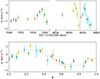 |
Fig. 1. Radial velocity curves determined for the observation summarised in Table 1. Top: Radial velocity vs. HJD. The vertical dotted line marks the switch from ESPaDOnS to SPIRou, and the different colours represent different rotation cycles. Bottom: Same as above, but folded in phase with P = 7.417 d and T0 = 2 457 544.40981. The dotted curve shows the sinus fit. |
where E is the rotation cycle. All our radial velocity measurements are in phase (Fig. 1), but the 2019 measurements show a larger amplitude of its modulation. This indicates that an evolving feature modulates the radial velocity, but that it was located at the same longitude in 2016 and 2019. The values are summarised in Table 2.
Radial velocities measured for each observation and their uncertainties.
3.2. Emission line variability
In this section, we present the analysis of the emission lines that either trace the accretion funnel flow, here, the Balmer lines (Muzerolle et al. 2001), or the accretion shock, such as the Ca II infrared triplet (IRT), the He I D3 (Beristain et al. 2001), or the He I at 1083 nm lines. For each line, we analysed the profile variability, their periodicity (except for the 2019 ESPaDOnS data set, which does not cover a sufficient time span), and the correlations of these variabilities. Most of the analyses of this section were performed using PySTEL(L)A1, a Python tool for SpecTral Emission Lines (variabiLity) Analysis.
3.2.1. Balmer lines
The Balmer lines are partly formed in the accretion funnel flow and therefore trace the magnetospheric accretion process. We focussed on Hα, Hβ, and Hγ, which we corrected for the photospheric contribution using the moderately active M-dwarf HD 42581 as template (Teff = 3822 K, v sin i = 2.6 km s−1, Manara et al. 2021), broadened to the v sin i of EX Lup. The 2016 and 2019 profiles are shown in Fig. 2 and Fig. 3, respectively. The profiles in both data sets are composed of a broad and a narrow component that are both highly variable. Furthermore, the flux is depleted below the continuum, around +200 km s−1, and extends up to +300 km s−1. This behaviour is characteristic of the so-called inverse P Cygni (IPC) profiles, the red-shifted absorption that forms by infalling material.
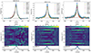 |
Fig. 2. Variability of 2016 Balmer lines of EX Lup. Top row: Hα(left), Hβ(middle), and Hγ(right) residual lines profiles. Each colour represents a different observation. Bottom row: 2D periodograms of the Hα(left), Hβ(middle), and Hγ(right) residual lines. The dotted white line marks the rotation period of 7.417 d. |
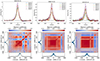 |
Fig. 3. Variability of the 2019 Balmer lines of EX Lup. Top row: Hα(left), Hβ(middle), and Hγ(right) residual lines profiles. Each colour represents a different observation. Bottom row: Hα(left), Hβ(middle), and Hγ(right) residual line auto-correlation matrices. The colour-code scales the correlation coefficient. Light yellow represents a strong correlation, and dark purple shows a strong anti-correlation. The strong anti-correlation around +350 km s−1 in the Hβ and Hγ matrices is probably an artefact because it is located in a part of the continuum that varies very little. |
The 2D periodograms, consisting of a Lomb-Scargle periodogram computed in each velocity channel, of the 2016 lines are presented in Fig. 2 and show a periodic signal along the whole Hβ and Hγ lines that is consistent with the rotation period of the star, with a false-alarm probability (FAP, computed from Baluev 2008, prescriptions) of 0.04 and 0.01, respectively. The Hα line shows this signal in a less continuous way with a much higher FAP (0.25). The symmetric signal around 0.9 d−1 is the one-day alias, a spectral leakage of the Fourrier transform that reconstructs (with the real period) the observation sampling, meaning approximately one observation per day.
To separate the various parts of the line profile that undergo different variability patterns, we computed the auto-correlation matrices of each line. This tool consists of computing a linear correlation coefficient (here, a Pearson coefficient) between the velocity channels of the line. A correlated region (close to 1) indicates a variability dominated by a given physical process. An anti-correlated region (close to −1) indicates a variability dominated by a given physical process or at least linked physical processes. The auto-correlation matrices of the 2019 Hα, Hβ, and Hγ lines are shown in Fig. 3. Here again, Hα behaves differently than Hβ and Hγ. Hα shows three main correlated regions between −100 km s−1 and +100 km s−1, corresponding to the core of the line, around +150 km s−1, corresponding to a slight emission excess in the IPC profile (occurring around HJD 2 458 8634.95 and 2 458 641.95), and around +250 km s−1, corresponding to the IPC profile itself. The two latter regions are anti-correlated, but the ∼+150 km s−1 region is also slightly anti-correlated with the line centre. This means that this region might be a broadening of the BC invoked by Sicilia-Aguilar et al. (2012), which causes a global decrease in the line (and accordingly an anti-correlation with the whole line profile). Hβ and Hγ show the same correlation around the line centre and +350 km s−1, without a significant anti-correlation around +150 km s−1, and a moderate anti-correlation of the profile with a region around +350 km s−1 which seems to be an artefact because it is located in the continuum.
3.2.2. He I D3 587.6 nm
The He I D3 lines of the 2016 and 2019 data sets are presented in Fig. 4 and are only composed of a narrow component (NC) that extends from approximately −35 to +50 km s−1, without significant BC. The NC is formed in the post-shock region of the accretion spot (Beristain et al. 2001) and can thus trace the accretion close to the stellar surface. This NC varies strongly and reaches maximum around ϕ = 0.62.
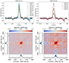 |
Fig. 4. EX Lup He I D3 line variability. Top row: 2016 (left) and 2019 (right) line profiles. Bottom row: Auto-correlation matrices of the 2016 (left) and 2019 (right) lines. |
The auto-correlation matrices shown in Fig. 4 confirm that this region is formed by one physical process, and the periodicity of the 2016 NC variation, consistent with the stellar rotation period (see Fig. 5, FAP = 0.06), indicates that this component traces an accretion shock at the stellar surface.
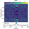 |
Fig. 5. He I D3 2016 2D periodogram. |
We thus performed a fit of the He I D3 NC radial velocity following the method described in Pouilly et al. (2021) to locate the emitting region. The results are shown in Fig. 6 and are summarised below:
 km s−1,
Vrot = 3.85 ± 5.0 km s−1,
dϕ = 0.10
 ,
,θ = 12.05
 °,
°,α = 55.40
 °,
°,
where Vflow is the velocity of the material in the post-shock region, Vrot is the equatorial velocity, 0.5+dϕ is the phase where the emitting region faces the observer, θ is the colatitude of the spot, and α = 90° −i, i is the inclination of the rotation axis. This means that the emitting region is located at ϕ = 0.6, 70° latitude. These results are consistent within the uncertainties with the measurements by Campbell-White et al. (2021), who reported for the He I emitting region3 a latitude of 60 ± 25°, longitude 40 ± 5°, meaning ϕ = 0.1 ± 0.01. However, the authors used the first date of observation as T0. Translated into our ephemeris (Eq. (1)), this yields ϕ = 0.7.
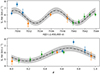 |
Fig. 6. Radial velocity fit of He I D3 2016 NC (top) and its version folded in phase (bottom) following the ephemeris given in Eq. (1). |
3.2.3. Ca II infrared triplet
Like the He I D3 NC, the Ca II IRT NC is formed in the post-shock region. We therefore studied these lines as well. The three components of this triplet show an identical shape and variability. We thus focussed on one of them that is located at 854.209 nm. The 2016 and 2019 residual line profiles are shown in Fig. 7 and Fig. 8, respectively. The two sets of lines show an IPC profile around 200 km s−1, which for the 2016 line is periodic with the stellar rotation period (see the 2D-periodogram in Fig. 7, FAP = 0.05).
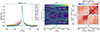 |
Fig. 7. ESPaDOnS 2016 Ca II IRT (854.2 nm) residual line profiles (left), 2D periodogram (middle), and auto-correlation matrix (right). |
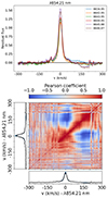 |
Fig. 8. ESPaDOnS 2019 Ca II IRT (854.2 nm) residual line profiles (top) and auto-correlation matrix (bottom). |
The 2016 auto-correlation matrix (Fig. 7) exhibits several correlated regions: from −130 to −60, −50 to −10, +50 to +100, +110 to +160, and +170 to +200 km s−1. However, there are fewer such regions in the 2019 matrix (Fig. 8), with only three correlated regions from −40 to +40, +80 to +130, and +150 to +200 km s−1, but we retrieved the correlated region around the IPC profile in both matrices, which is anti-correlated with the NC in 2019. This agrees with the smaller (larger) variability in the NC (BC) that was observed in 2016 compared to 2019, showing the different origins of the two components and a small change in the accretion pattern between the two epochs.
3.2.4. He I 1083 nm
The only accretion tracer in emission in the EX Lup SPIRou observation is the He I line at 1083 nm. The profiles, the 2D periodogram, and the auto-correlation matrix are shown in Fig. 9. The profiles appear to be composed of two peaks that are blue- and red-shifted around −50 and +100 km s−1, and two absorptions that are blue-and red-shifted at a higher velocity (−150 and +200 km s−1).
 |
Fig. 9. SPIRou He I (1083 nm) line profiles (left), 2D periodogram (middle), and auto-correlation matrix (right). |
The red-shifted peak and the two absorptions display significant variability and seem modulated on the stellar rotation period. The FAPs reach 0.001, 0.01, and 0.02 for the red-shifted peak, the blue- and the red-shifted absorption, respectively.
The auto-correlation matrix revealed a more complex decomposition. When the four substructures seen in the profiles are represented, the two absorptions both appear to be separated into two regions, from −250 to −160 and −160 to −110 km s−1 for the blue-shifted absorption, and from +130 to +170 km s−1 and +210 to +270 km s−1 for the red-shifted absorption. Furthermore, the main peak at ∼+100 km s−1 is anti-correlated with the most blue- and red-shifted regions only. This can be interpreted as follows: The blueshifted absorption, probably a P-Cygni profile traditionally ascribed to a wind, is also associated with a redshifted emission excess that produces the two substructures seen in the redshifted absorption. The IPC profile, as the opposite physical phenomenon, is also associated with a blueshifted emission excess that causes the two substructures in the blue-shifted absorption.
3.2.5. Correlation matrices ESPaDOnS
As the several lines we studied trace different accretion regions, we computed correlation matrices between two different lines to analyse the link between the different regions we identified from the auto-correlation matrices. The correlation matrices of the 2016 and 2019 lines are presented in Appendix A.
In 2016, the Hα line centre is correlated with the He I D3 and the Ca II IRT NCs, and it is slightly anti-correlated with the region of Ca II IRT IPC profile. The latter is also strongly anti-correlated with the He I D3 NC. The region of the Hα IPC profile is also anti-correlated with the He I D3 NC, and it is correlated with the region of the Ca II IRT IPC profile. The 2019 matrices show the same between the NCs and IPC regions of the various lines, but both the correlation and anti-correlation coefficients are stronger.
3.3. Magnetic field
In this section, we present the magnetic analysis of EX Lup. We analysed it at two scales: at the large scale using the Zeeman-Doppler imaging technique (ZDI, Donati et al. 2011), and at the small scale using the Zeeman intensification of photospheric lines.
3.3.1. Large scale
In this section, we use the least-squares deconvolution method (LSD, Donati et al. 1997; Kochukhov et al. 2010) to study the large-scale magnetic field. This method allows us to increase the S/N of the Stokes I (unpolarised) and Stokes V (circularly polarised) profiles by using as many photospheric lines as possible. To compute the LSD profiles, we used the LSDpy4 Python implementation. We normalised our LSD weights using an intrinsic line depth, a mean Landé factor, and a central wavelength of 0.2, 1.2, and 500 nm (respectively) for ESPaDOns, and 0.1, 1.2, and 1700 nm for SPIRou observations. The photospheric lines were selected from a mask that was produced using the same VALD line list and MARCS atmospheric models as in Sect. 3.1, and we removed the emission lines, the telluric and the heavily blended lines regions with the SpecpolFlow5 Python package. About 12 000 lines were used for ESPaDOnS, and 1600 lines were used for SPIRou observations. The LSD profiles of the ESPaDOnS 2016 and 2019 and of the SPIRou observations are presented in Figs. 10, 11, and 12, respectively, and the S/Ns of the profiles are available in Table 1. The observation at HJD 2 457 551.87135 was removed from this analysis because of its low S/N.
 |
Fig. 10. ESPaDOnS 2016 LSD Stokes I(left) and V(right) profiles. The rotation phase and the HJD are indicated left and right of each profile, respectively. The scale is indicated in the bottom left corner of each plot. |
A clear Stokes V signature is detected for all ESPaDOnS observations and for most of the SPIRou observations. Furthermore, the SPIRou Stokes V signatures are much weaker than ESPaDOnS, and the signal at ϕ ∼ 0.6–0.7 almost vanishes on SPIRou when it is highest on ESPaDOnS.
The surface-averaged longitudinal magnetic field can be directly estimated from the LSD profiles (Bℓ, Donati et al. 1997; Wade et al. 2001),
 (2)
(2)
where Bℓ is in Gauss, v is the velocity relative to the line centre, and λ and g are the central wavelength and the mean Landè factor we used for the LSD computation. The integration was performed on a ±25 km s−1 (±35 km s−1) velocity range around the stellar rest frame to minimise the uncertainties without losing any magnetic information on the ESPaDOnS (SPIRou) observations. The Bℓ curves are shown in Fig. 13. The three curves are modulated with the stellar rotation period and are highest around ϕ = 0.6. In the optical frame, the modulation amplitude is slightly larger in 2019 than in 2016, which is reminiscent of the radial velocity behaviour (see Sect. 3.1). Finally, as expected from the Stokes V signatures, the SPIRou measurements are far weaker and mostly negative.
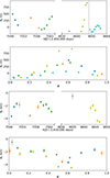 |
Fig. 13. Bℓ curves from LSD profile (top two panels) and from He I D3 line (bottom two panels). |
The same analysis can be performed on the NC of the He I D3 line (on a ±50 km s−1 velocity range), which is formed close to the accretion shock and thus gives access to the magnetic field strength at the foot of the accretion funnel flow. The Bℓ obtained are shown in Fig. 13 and range between −1.4 and −3.7 kG in 2016 and between −0.5 and −4.5 kG in 2019. The modulation amplitude of the Bℓ is larger in 2019, which is reminiscent of the radial velocity behaviour (see Sect. 3.1), but both curves are in phase. A minimum is reached at ϕ = 0.6, which is also consistent with the position of the emitting region we obtained from the radial velocity modulation of the He I D3 NC (see Sect. 3.2.2). These measurements are also opposite in phase and sign with the LSD Bℓ. This is a common behaviour on cTTSs (e.g., see the studies of S Cra N, TWA Hya, CI Tau by Nowacki et al. 2023; Donati et al. 2011, 2020a, respectively) that reflects that LSD and He I D3 NC diagnostics probe different regions of different polarities.
Finally, we performed a complete ZDI analysis of the three data sets using ZDIpy6 (described in Folsom et al. 2018) with a recent implementation of Unno-Rachkovsky’s solutions to polarised radiative transfer equations in a Milne-Eddington atmosphere (Unno 1956; Rachkovsky 1967; Landi Degl’Innocenti & Landolfi 2004) as presented in Bellotti et al. (2023) to use a more general description than the weak-field approximation used initially in ZDIpy. The magnetic topology was reconstructed in two steps: (i) the building of a Doppler image (DI), starting from a uniformly bright stellar disk and iteratively adding dark and bright features to fit the observed LSD Stokes I profiles, and (ii) fitting the LSD Stokes V profiles to derive the magnetic topology by adjusting its spherical harmonic components (Donati et al. 2006), with a maximum degree of harmonic expansion ℓmax = 15 here. We used as input parameter Prot = 7.417 d, v sin i = 4.4 km s−1. We then ran a grid of ZDI Stokes V reconstructions over the inclination range derived in the literature (20–45°) and used the lowest χ2 obtained to set our input inclination value (i = 30°). The resulting maps are presented in Figs. 14 and 15, and the corresponding LSD profile fits are shown in Appendix B.
 |
Fig. 14. Brightness maps from the ESPaDOnS 2016, 2019, and SPIRou data sets (left, middle, and right, respectively) on a flattened polar view. The central dot is thus the pole, the two dotted circles are latitude 60 and 30°, and the solid circle represents the equator. The black ticks show the clockwise rotation phases, and the red ticks represent the observed phases. The colour-code indicates the brightness on a linear scale, where a value of 1.0 represents the quiet photosphere. Values lower than one are darker regions, and values greater than one are bright. |
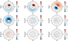 |
Fig. 15. Radial (top row), azimuthal (middle row), and meridional (bottom row) magnetic maps from the ESPaDOnS 2016, 2019, and SPIRou data sets (left, middle, and right columns, respectively) in the same flattened polar view as Fig. 14. The colour-code scales the magnetic field strength from dark blue for the strongest negative value to dark red for the strongest positive value. |
The ESPaDOnS 2016 DI map shows a main dark spot around ϕ = 0.55 that extends between 70 and 20° latitude, which is consistent with He I D3 emitting region, and a bright structure from ϕ = 0.95 to 0.20 around the equator that is certainly a plage, as even the accretion shock is dark at the photospheric level. The magnetic topology, mostly toroidal (61%), is dominated by the dipolar (60%) and quadrupolar (17%) components, with a mean magnetic field strength of 1.00 kG (Bmax = 3.12 kG) and a magnetic dipolar positive pole of 0.728 kG located at about 30° latitude and 166° longitude (ϕ = 0.46).
The brightness map obtained from SPIRou revealed a main dark feature extended from ϕ = 0.0 to 0.25 and a bright plage around ϕ = 0.6, which is perfectly consistent with the 2016 map. However, the magnetic topology seems to be less complex than in 2016. It is almost fully poloidal (99%) and more dominated by the dipole component (77%). As expected, the recovered field strength is much smaller (⟨B⟩ = 0.131 kG, Bmax = 0.389 kG). The dipole negative pole is located at about 23° latitude, 329° longitude (ϕ = 0.91), with a −0.231 kG-strength.
Given the poor rotational phase coverage of the ESPaDOnS 2019’s data set (ϕ∈ [0.03, 0.64]), we needed to guide the reconstruction instead of starting from a uniform map to avoid a too strong extrapolation on the missing phases. We do not expect a similar brightness contrast between ESPaDOnS and SPIRou, but given the very similar spectroscopic behaviour between the 2016 and 2019 ESPaDOnS data sets (see Sects. 3.1 and 3.2), we might expect similar features. We therefore used the ESPaDOnS 2016 brightness map as input to guide its reconstruction. To check this assumption, we reproduced the Stokes I profiles resulting from the 2016 reconstruction on the 2019 phases, yielding a consistent behaviour (reduced χ2 = 1.1). The obtained final brightness reconstruction shows a main dark feature that is slightly shifted in phase compared to 2016 (ϕ ≈ 0.5) and less extended in latitude. A polar bright feature is also located around ϕ = 1, which is reminiscent of the SPIRou maps. We expect a similar topology of the magnetic field between SPIRou and ESPaDOnS 2019 for the magnetic reconstruction, with different magnetic strengths, as pointed out by the Bℓ analysis. We therefore used the SPIRou magnetic maps as input to guide the reconstruction. The resulting topology is less poloidal-dominated than SPIRou (91%), and the dipolar component occupies a smaller fraction of this poloidal field (65%), with a similar contribution of the quadrupolar and octupolar components (about 15%). Surprisingly, the mean magnetic field strength is similar to 2016 (1.08 kG), but the maximum field strength is much higher (4.79 kG), as is the strength of the dipolar pole Bdip = 1.87 kG, which is located at the same position (ϕ = 0.43 and 30° latitude).
3.3.2. Small scale
Even though the ZDI analysis gives access to the magnetic topology, it neglects the small-scale magnetic field, which contains a major part of the magnetic energy of cool stars. This is analysed by studying the change it induces in the shape of magnetically sensitive lines (Kochukhov et al. 2020). This technique is called Zeeman intensification. To perform this analysis, we used the algorithm of Hahlin et al. (2021), performing a Markov chain Monte Carlo (MCMC) sampling, using the SoBaT library (Anfinogentov et al. 2021) on a grid of synthetic spectra produced by the SYNMAST code. This polarised radiative transfer code was described by Kochukhov et al. (2010). This grid was computed from the VALD line lists used in Sect. 3.1 and from MARCS atmospheric models (Gustafsson et al. 2008). We parametrised a uniform radial magnetic field as the sum of the magnetic field strength ranging from 0 to 6 kG with a step of 2 kG, weighted by filling factors representing the amount of stellar surface covered by this magnetic field. For the ESPaDOnS observations, as in previous studies (Hahlin & Kochukhov 2022; Pouilly et al. 2023, 2024), we used the 963.5–981.2 nm region.
This region contains a group of Ti I lines with different magnetic sensitivity (geff summarised in Table 3), allowing us to disentangle the effect of the magnetic field on the equivalent widths from the effect of any other parameters, such as the Ti I abundance. However, this region also contains many telluric lines that are superimposed on the Ti I lines from the stellar spectra and which need to be removed from the observed spectrum for the magnetic analysis. To do this, we used the molecfit package (Smette et al. 2015), which was developed to model and remove telluric lines from spectra obtained with instruments at the European Southern Observatory. It can be used on spectra from any instrument.
Ti I lines used for the Zeeman intensification analysis.
Finally, as EX Lup is an accreting star with the signature of an accretion shock, the veiling might disturb the inference results, in particular, the abundance, the v sin i and the radial tangential macroturbulent velocity, vmac. We thus estimated the veiling using the magnetic null line of the Ti I multiplet at 974.36 nm by performing a χ2 minimisation using SYNMAST synthetic spectra. We let the abundance, the v sin i, and the vmac as free parameters and added a fractional veiling, defined as
 (3)
(3)
where Iveil is the veiled spectrum, I is the spectrum without veiling, and r is the fractional veiling. We stress that deriving a precise value of the veiling is beyond the scope of this study.
Our aim was to estimate the EX Lup mean spectrum at a wavelength close to the Ti I lines in order to minimise its effect on the other inferred parameters. For the 2016 ESPaDOnS mean spectrum, the minimum χ2 is reached for r = 0.5, v sin i = 4.9 km s−1, vmac = 1.9 km s−1, and a Ti I abundance of −7.2. For the mean spectrum of the 2019 ESPaDOnS observations, we obtained r = 0.48, v sin i = 5.0 km s−1, vmac = 2.5 km s−1, and a Ti I abundance of −7.2. We therefore assumed the values obtained for r and vmac, and used the others as initial guesses for the MCMC sampling.
We assumed a multicomponent model given by
 (4)
(4)
where fi are the filling factors, that is, the fraction of the stellar surface covered by a field strength Bi, and Si are the synthetic spectra of the corresponding magnetic field strength. The averaged magnetic field is thus given by
 (5)
(5)
To set the number of the filling factor to be used, we iteratively added filling factors with a step of 2 kG in the corresponding magnetic field strength, and used the Bayesian information criterion (BIC, Sharma 2017) to only include the filling factors that significantly improved the fit. The suitable solutions are components of 0, 2, and 4 kG for the ESPaDOnS 2016 and SPIRou observations, and 0, 2, 4, 6, and 8 kG for ESPaDOnS 2019. The free parameters of the analysis are thus the following: fi, v sin i, vr, and the Ti I abundance, for which uniform priors were adopted. Finally, we used an effective sample size of 1000 (Sharma 2017).
The resulting line fit and magnetic field strength posterior distributions are presented in Fig. 16. The 2016 magnetic field strength (3.08 ± 0.04 kG) is consistent with that from 2019 within the uncertainties (3.16 ± 0.05 kG). The inferences of all parameters are summarised in Table 4.
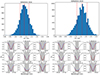 |
Fig. 16. Results of the ESPaDOnS Zeeman intensification analysis. Top: Distribution of the average magnetic field of EX Lup for the 2016 (left) and 2019 (right) data sets. The solid red line represents the median, and the dashed lines represent the 68 % confidence regions. Bottom: Fit to 2016 (left) and 2019 (right) optical Ti I multiplet of EX Lup. The solid red line shows the best fit to the observations in black, while the dashed blue line shows the non-magnetic spectra with otherwise identical stellar parameters. The shaded area marks the region used for the fit. |
Inference results on the small-scale magnetic field on Ti I lines.
For SPIRou observations, we again used a set of Ti I lines around 2200 nm (see Table 3). Unfortunately, this wavelength region does not contain any magnetically null line that is deep enough at our S/N to perform the veiling study we performed on ESPaDOnS observations. Only a visual inspection of the line at 974.4 nm is possible, indicating that the parameters obtained for ESPaDOnS at this wavelength are consistent with the SPIRou observations. We thus used the veiling values obtained for the 2019 ESPaDOnS data set, fixed the v sin i at the literature value, and let the inference compensate for the eventual error with the non-magnetic parameters. The inferred parameters are summarised in Table 4, and the line fit and inferred magnetic field strength are shown in Fig. 17. The magnetic field strength we recovered (2.00 ± 0.03 kG) is significantly lower than the values found for the ESPaDOnS observations. As highlighted by Hahlin et al. (2023), the small-scale field might be overestimated in the optical wavelength. In our case, a second explanation might come from the high vmac we obtained, which is probably needed to compensate for an underestimated veiling. This lowers the effect of the magnetic field.
4. Discussion
We characterised the accretion process of the prototypical EXor, EX Lup, in quiescence, together with its magnetic field at small and large scales. We confirmed that the typical magnetospheric accretion process of cTTSs is ongoing in this system, which seems stable between the two epochs we studied (2016 and 2019). A main accretion funnel flow connects the disc to the stellar surface. This produces the IPC profile observed in the H lines we studied and their modulation with the stellar rotation period. The accretion shock at the stellar surface produces the emission of the NC of the He I D3 and Ca II IRT lines, which are modulated with the stellar period and are anti-correlated with the IPC profiles, as expected in the magnetospheric accretion scheme. This is consistent with the occurrence of the maximum IPC profile at the same phase as the He I D3 emitting region (ϕ≈ 0.6), indicating a funnel flow that is aligned with the accretion shock, and inherently meaning that the truncation radius is located at the stellar corotation radius. As expected, this phase is also associated with an extremum of Bℓ for both LSD and He I D3 measurements, and with the ESPaDOnS ZDI brightness and magnetic topology reconstructions, showing the connection between accretion and magnetic field. To investigate the truncation radius rmag, we used the expression given by Bessolaz et al. (2008),
 (6)
(6)
where the Mach number ms ≈ 1, B⋆ is the equatorial magnetic field strength (given from the dipole strength and the relation of Gregory 2011) in units of 140 G, Ṁacc is the mass accretion rate in units of 10−8 M⊙⋅yr−1, M⋆ is the stellar mass in units of 0.8 M⊙, and R⋆ is the stellar radius in units of 2 R⊙. As Ṁacc in quiescence, we used the value before the 2022 outburst given by Wang et al. (2023), 1.8 × 10⁻⁹ M⊙⋅yr−1. The stellar mass and radius are given by Gras-Velázquez & Ray (2005) (0.6 M⊙ and 1.6 R⊙), and the magnetic obliquity is obtained from the ZDI analysis (30° for ESPaDOnS, 23° for SPIRou; see Sect. 3.3.1). The dipole strengths needed to obtain rmag = rcorot = 8.5 ± 0.5 R⋆ are thus 2.10 ± 0.46 kG and 1.98 ± 0.43 kG for ESPaDOnS and SPIRou, respectively. Only an estimate of the truncation radius was obtained because we lack a precise value of the dipole strength. The Bℓ measurements in the He I D3 line and the Zeeman intensification values also contain the higher-order components of the magnetic field, and the ZDI spherical harmonic decomposition from LSD might include flux cancellation that lowers the large-scale strength we obtained. Even though the ZDI results on the 2019 datasets indicate a topology that is largely dominated by the dipole component, using these values should yield an overestimation of rmag. The results using our magnetic field measurements are summarised in Table 5. The values we obtained from the Bℓ and the small-scale field are not consistent with the corotation radius, as expected, except for the SPIRou measurement. This can be explained by the smaller recovered field in the infrared domain. However, the optical ZDI values yield truncation radii consistent with the corotation radius because the dipole-dominant magnetic topology of the system allowed us to recover a good estimate of the dipole pole strength using ZDI. Here again, the SPIRou value yields a lower truncation radius due to the lower magnetic field strength obtained.
Magnetospheric truncation radius obtained using the various magnetic field measurements.
The difference in the results of the various magnetic analyses between the optical and infrared frames in 2019 needs to be discussed. From the Bℓ computed from the LSD profiles, the maximum values obtained are 911 ± 26 and 64 ± 20 G for the ESPaDOnS and SPIRou observations, respectively. These maxima both occurred around ϕ = 0.6, where the Stokes V signature is strongest with ESPaDOnS but almost vanishes with SPIRou. A large discrepancy here is therefore expected. The minimum Bℓ values reach −155 ± 11 and −178 ± 13 G for the ESPaDOnS and SPIRou observations, respectively. They are both around ϕ = 0.1 and are thus consistent. This behaviour is also visible in the ZDI reconstruction, where the strong positive radial magnetic field region at phase 0.6 in the ESPaDOnS map completely vanishes in the SPIRou map. The two qualitative explanations we can provide are the following: (i) This maximum value is located in an optically dark region of the photosphere, which is consistent with simultaneous optical photometry (Kóspál et al., in prep.), and it is thus less contrasted in the SPIRou domain. The magnetic contribution of this region to the Stokes V signal might therefore be lowered in the infrared domain when the smaller-scale negative field is obscured in the optical domain. Furthermore, (ii) the two wavelength domains allow us to trace different heights in the photosphere, and this difference might be an indication of a vertical structure of the magnetic field.
The two ZDI reconstructions we obtained from the two ESPaDOnS epochs appear to indicate similar brightness and magnetic radial maps even though the overall topology has evolved from a toroidal- to a poloidal-dominated state, as was reported previously (e.g., DQ Tau A, Pouilly et al. 2023, 2024). The strong positive radial field spot that is associated with the dark spot of the stellar brightness and with the dipole pole is also consistent with the modulation of the He I D3 NC radial velocity and Bℓ. However, the latter indicates an accretion shock associated with a region with a strong negative field. Given the large amplitude of the He I D3 NC radial velocity variation compared to EX Lup v sin i, the emitting region is probably very small, meaning that its magnetic field information is lost at the photospheric level. This might explain this disparity (Yadav et al. 2015).
Despite this stable pattern between 2016 and 2019, we observed some disparities in some parameters. Even though the radial velocity and the Bℓ (from LSD and He I D3) modulations are well in phase, their amplitudes are slightly larger in 2019. If the stronger magnetic field obtained in the optical frame at the small and large scale explains the larger amplitude of the Bℓ modulation, the accompanying effect on the radial velocity indicates a modulation by the hotspot. This is an expected behaviour, but the consistency between the ESPaDOnS and SPIRou radial velocity measurements is surprising. The stellar activity effect on the photospheric lines that produce the apparent radial velocity modulation is a wavelength-dependent phenomenon. An amplitude consistency between the radial velocity measurements in the optical and infrared frames is thus not expected.
To investigate in our data sets the relation between the stellar activity and the radial velocity modulation, we compared the latter to an activity indicator, the bisector inverse slope (BIS, Queloz et al. 2001). The BIS was computed from the LSD profiles presented in Figs. 10, 11, and 12, and it is defined as the difference between the mean velocity of the bisector at the top and bottom of the line. In the ESPaDOnS profiles, the first 15%, which contain the continuum and the wings, were ignored, as were the last 15%, where the noise or an activity signature splitting the profile into two parts can affect the computation. The top and bottom regions we used to compute the BIS are the top and bottom 25% parts of the remaining profile. For the SPIRou profiles, the same conditions were used, but we had to ignore the first 25% of the profiles as it was affected by stronger wings. When the radial velocity modulation is only induced by the stellar activity, the line deformation, indicated by the BIS, entirely causes this modulation. This means that a strong linear correlation should appear between the BIS and the radial velocity, in a perfect situation, with a −1-slope and a BIS = 0 km s−1 at the mean velocity.
The plots of BIS versus radial velocity are presented in Appendix C. For each data set, the Pearson correlation coefficient indicates a strong anti-correlation (2016: r = −0.81, p-value = 0.005; ESPaDOnS 2019: r = −0.95, p-value = 0.004; SPIRou: r = −0.72, p-value = 0.05). However, the optical measurements show much shallower slopes (−0.51 ± 0.13 and −0.43 ± 0.07 in 2016 and 2019, respectively) and an intersect far from the mean velocity expected (−0.34 ± 0.10 and −0.08 ± 0.06). Only the infrared measurements are consistent (slope:−0.68 ± 0.27, intersect: −1.37 ± 0.25), but only because of the larger uncertainties that are probably due to the lower correlation. Furthermore, the much lower BIS we obtained (exclusively negative) in the infrared compared to the optical frame indicates chromatic effects that are not observed in the radial velocity modulation. Stellar activity therefore probably dominates the radial velocity modulation, but another effect, such as Doppler shift induced by a companion, cannot be completely excluded and needs further investigations. These are unfortunately beyond the scope of this work.
Finally, we would like to address the strong magnetic field we recovered that drives the accretion process on EX Lup. With Bℓ reaching 4.2 kG in the accretion shock, a dipole strength of 1.9 kG within a large-scale field of 1 kG reaching 4.8 kG locally, and a small-scale field exceeding 3 kG in the optical domain, EX Lup has one of the strongest magnetic field of all cTTSs, and the strongest of those with a dipole-dominated topology. This configuration can set the suitable condition invoked by D’Angelo & Spruit (2010) for their hypothesis of an episodic accretion due to the magnetospheric accretion process itself. With this dipolar strength, the magnetospheric radius is outside of but close to the corotation radius (see Table 5). In this situation, instability arises because angular momentum is transferred from the star to the disc (the so-called propeller regime), but it is not enough to drive an outflow. This magnetic interaction only prevents accretion, pilling up the gas in the inner disc and increasing its pressure. It therefore forces the inner edge of the disc to move inward and cross the corotation radius. This allows accretion to occur. After the gas reservoir has been accreted, the inner edge of the disc moves outward and another cycle starts (see D’Angelo & Spruit 2010; D’Angelo & Spruit 2011; D’Angelo & Spruit 2012). This phenomenon is different from the magnetospheric inflation reported for other cTTSs (e.g., see the studies of AA Tau or V807 Tau by Bouvier et al. 2003; Pouilly et al. 2021, respectively), where a significant difference between the truncation and corotation radii induces a torsion of the magnetic field lines, which in turn produces a toroidal field that inflates the whole magnetosphere. This inflation reaches an opening of the magnetic field lines that produces a magnetospheric ejection (Zanni & Ferreira 2013; Pantolmos et al. 2020) before reconnecting to the disc. This phenomenon is recurrent and produces an accretion variability as well. Still, the timescale of this cycle is of the order of the stellar rotation period, far shorter than the gas pile-up invoked by D’Angelo & Spruit (2010), and no signature of magnetospheric inflation or ejection was detected in EX Lup. However, we would like to stress that no accumulation of matter at the magnetospheric radius was detected either. EX Lup only appears to be in the same initial conditions as the latter authors’ theory. In addition, the BIS suggest another source for radial velocity variation, such as a companion. Tidal interactions (Bonnell & Bastien 1992) or thermal instabilities in the disc (Lodato & Clarke 2004) induced by a companion are also existing hypotheses for the EXor behaviour. Moreover, recent works by Nayakshin et al. (2024b,a) favoured the latter instability as the origin of the episodic accretion of FUor objects. Finally, the disc itself was not investigated in this work. Instabilities in the disc are thus hypotheses that cannot be excluded (Bell & Lin 1994; Armitage et al. 2001).
5. Conclusions
EX Lup is the prototypical EXor-type object. Its recurrent bursts and outbursts were previously studied in detail using spectroscopy and photometry. However, no information about its magnetic field was derived before, despite its key role in the accretion process of cTTS and even though it might be the origin of episodic accretion. We provided the first spectropolarimetric time-series study over two epochs (2016 and 2019) and two wavelength domains (optical and infrared) of EX Lup. This is the first EXor whose magnetic field was studied.
We confirmed an ongoing magnetospheric accretion process as seen in many cTTSs. It is represented by an accretion funnel flow and an accretion shock that corotates with the stellar surface and is driven by a kG dipolar magnetic field. The funnel flow seems to be aligned with the accretion shock, which itself is located near the magnetic dipole pole. This is consistent with the stable pattern that is observed between the epochs we studied.
The magnetic field of EX Lup has shown some disparities between the wavelength domains, which are much weaker in the infrared. This can be understood as a wavelength dependence of the parameters we studied, but it can also indicate a vertical structure of the magnetic field because different wavelengths trace different heights in the photosphere. An expected small- to large-scale effect is also observed based on the different field strengths we recovered using ZDI and Zeeman intensification, but also based on the opposite polarity of the field associated with the accretion shock and the field recovered using LSD. This indicates a very small accretion shock, as expected from the low mass accretion rate in quiescence and the large radial velocity variation of the emitting region.
Finally, the multi-kilogauss field we recovered for EX Lup indicates that the magnetospheric radius is close to but larger than the corotation radius. This configuration is suitable for disc instabilities induced by the magnetic field that yield accretion cycles. These cycles might explain the accretion bursts observed on EX Lup, suggesting an inherently episodic magnetospheric accretion process. However, a definite identification of the origin of EXor behaviour is beyond the scope of this paper, and other theories implying the disc itself or a companion cannot be excluded.
Data availability
The Espadons and Spirou reduced polarimetric spectra is available at the CDS via anonymous ftp to cdsarc.cds.unistra.fr (130.79.128.5) or via https://cdsarc.cds.unistra.fr/viz-bin/cat/J/A+A/691/A18
HJD 2 457 548.91, 2 458 645.88, and 2 458 646.87.
Values estimated from their Fig. 7.
Acknowledgments
We would like to warmly thanks Oleg Kochukhov for useful discussions about the magnetic field of EX Lup, as well as Colin P. Folsom for his help in using the new version of his ZDIpy package. The SpecpolFlow package is available at https://github.com/folsomcp/specpolFlow. The PySTEL(L)A package is available at https://github.com/pouillyk/PySTELLA This research was funded in whole or in part by the Swiss National Science Foundation (SNSF), grant number 217195 (SIMBA). For the purpose of Open Access, a CC BY public copyright licence is applied to any Author Accepted Manuscript (AAM) version arising from this submission. Based on observations obtained at the Canada–France– Hawaii Telescope (CFHT) which is operated from the summit of Maunakea by the National Research Council of Canada, the institut National des Sciences de l’Univers of the Centre National de la Recherche Scientifique of France, and the University of Hawaii. The observations at the Canada–France–Hawaii Telescope were performed with care and respect from the summit of Maunakea which is a significant cultural and historic site. This work was also supported by the NKFIH excellence grant TKP2021-NKTA-64.
References
- Anfinogentov, S. A., Nakariakov, V. M., Pascoe, D. J., & Goddard, C. R. 2021, ApJS, 252, 11 [Google Scholar]
- Armitage, P. J., Livio, M., & Pringle, J. E. 2001, MNRAS, 324, 705 [NASA ADS] [CrossRef] [Google Scholar]
- Audard, M., Ábrahám, P., Dunham, M. M., et al. 2014, in Protostars and Planets VI, eds. H. Beuther, R. S. Klessen, C. P. Dullemond, & T. Henning, 387 [Google Scholar]
- Baluev, R. V. 2008, MNRAS, 385, 1279 [Google Scholar]
- Bell, K. R., & Lin, D. N. C. 1994, ApJ, 427, 987 [NASA ADS] [CrossRef] [Google Scholar]
- Bellotti, S., Morin, J., Lehmann, L. T., et al. 2023, A&A, 676, A56 [NASA ADS] [CrossRef] [EDP Sciences] [Google Scholar]
- Beristain, G., Edwards, S., & Kwan, J. 2001, ApJ, 551, 1037 [Google Scholar]
- Bessolaz, N., Zanni, C., Ferreira, J., Keppens, R., & Bouvier, J. 2008, A&A, 478, 155 [NASA ADS] [CrossRef] [EDP Sciences] [Google Scholar]
- Bonnell, I., & Bastien, P. 1992, ApJ, 401, L31 [Google Scholar]
- Bouvier, J., Grankin, K. N., Alencar, S. H. P., et al. 2003, A&A, 409, 169 [NASA ADS] [CrossRef] [EDP Sciences] [Google Scholar]
- Campbell-White, J., Sicilia-Aguilar, A., Manara, C. F., et al. 2021, MNRAS, 507, 3331 [NASA ADS] [CrossRef] [Google Scholar]
- Cook, N. J., Artigau, É., Doyon, R., et al. 2022, PASP, 134, 114509 [NASA ADS] [CrossRef] [Google Scholar]
- Cruz-Sáenz de Miera, F., Kóspál, Á., Abrahám, P., et al. 2023, A&A, 678, A88 [NASA ADS] [CrossRef] [EDP Sciences] [Google Scholar]
- D’Angelo, C. R., & Spruit, H. C. 2010, MNRAS, 406, 1208 [NASA ADS] [Google Scholar]
- D’Angelo, C. R., & Spruit, H. C. 2011, MNRAS, 416, 893 [CrossRef] [Google Scholar]
- D’Angelo, C. R., & Spruit, H. C. 2012, MNRAS, 420, 416 [Google Scholar]
- Donati, J.-F. 2003, ASP Conf. Ser., 307, 41 [Google Scholar]
- Donati, J.-F., Semel, M., Carter, B. D., Rees, D. E., & Collier Cameron, A. 1997, MNRAS, 291, 658 [NASA ADS] [CrossRef] [Google Scholar]
- Donati, J.-F., Howarth, I. D., Jardine, M. M., et al. 2006, MNRAS, 370, 629 [NASA ADS] [CrossRef] [Google Scholar]
- Donati, J. F., Gregory, S. G., Alencar, S. H. P., et al. 2011, MNRAS, 417, 472 [NASA ADS] [CrossRef] [Google Scholar]
- Donati, J. F., Bouvier, J., Alencar, S. H., et al. 2020a, MNRAS, 491, 5660 [Google Scholar]
- Donati, J. F., Kouach, D., Moutou, C., et al. 2020b, MNRAS, 498, 5684 [Google Scholar]
- Fischer, W. J., Hillenbrand, L. A., Herczeg, G. J., et al. 2023, ASP Conf. Ser., 534, 355 [NASA ADS] [Google Scholar]
- Folsom, C. P., Bagnulo, S., Wade, G. A., et al. 2012, MNRAS, 422, 2072 [NASA ADS] [CrossRef] [Google Scholar]
- Folsom, C. P., Bouvier, J., Petit, P., et al. 2018, MNRAS, 474, 4956 [NASA ADS] [CrossRef] [Google Scholar]
- Gaia Collaboration (Vallenari, A., et al.) 2023, A&A, 674, A1 [NASA ADS] [CrossRef] [EDP Sciences] [Google Scholar]
- Goto, M., Regály, Z., Dullemond, C. P., et al. 2011, ApJ, 728, 5 [CrossRef] [Google Scholar]
- Gras-Velázquez, À., & Ray, T. P. 2005, A&A, 443, 541 [NASA ADS] [CrossRef] [EDP Sciences] [Google Scholar]
- Gregory, S. G. 2011, Am. J. Phys., 79, 461 [NASA ADS] [CrossRef] [Google Scholar]
- Gustafsson, B., Edvardsson, B., Eriksson, K., et al. 2008, A&A, 486, 951 [NASA ADS] [CrossRef] [EDP Sciences] [Google Scholar]
- Hahlin, A., & Kochukhov, O. 2022, A&A, 659, A151 [NASA ADS] [CrossRef] [EDP Sciences] [Google Scholar]
- Hahlin, A., Kochukhov, O., Alecian, E., & Morin, 2021, J., & BinaMIcS Collaboration, A&A, >650, A197 [NASA ADS] [CrossRef] [EDP Sciences] [Google Scholar]
- Hahlin, A., Kochukhov, O., Rains, A. D., et al. 2023, A&A, 675, A91 [NASA ADS] [CrossRef] [EDP Sciences] [Google Scholar]
- Hartmann, L., Herczeg, G., & Calvet, N. 2016, ARA&A, 54, 135 [Google Scholar]
- Kochukhov, O., Makaganiuk, V., & Piskunov, N. 2010, A&A, 524, A5 [NASA ADS] [CrossRef] [EDP Sciences] [Google Scholar]
- Kochukhov, O., Hackman, T., Lehtinen, J. J., & Wehrhahn, A. 2020, A&A, 635, A142 [NASA ADS] [CrossRef] [EDP Sciences] [Google Scholar]
- Kóspál, Á., Mohler-Fischer, M., Sicilia-Aguilar, A., et al. 2014, A&A, 561, A61 [NASA ADS] [CrossRef] [EDP Sciences] [Google Scholar]
- Landi Degl’Innocenti, E., & Landolfi, M. 2004, in Polarization in Spectral Lines, (Kluwer Academic Publishers), Astrophys. Space Sci. Lib., 307 [Google Scholar]
- Landstreet, J. D. 1988, ApJ, 326, 967 [Google Scholar]
- Lodato, G., & Clarke, C. J. 2004, MNRAS, 353, 841 [NASA ADS] [CrossRef] [Google Scholar]
- Manara, C. F., Frasca, A., Venuti, L., et al. 2021, A&A, 650, A196 [NASA ADS] [CrossRef] [EDP Sciences] [Google Scholar]
- Muzerolle, J., Calvet, N., & Hartmann, L. 2001, ApJ, 550, 944 [Google Scholar]
- Nayakshin, S., Cruz Sáenz de Miera, F., & Kóspál, Á. 2024a, MNRAS, 532, L27 [NASA ADS] [CrossRef] [Google Scholar]
- Nayakshin, S., Cruz Sáenz de Miera, F., & Kóspál, Á. 2024b, MNRAS, 530, 1749 [NASA ADS] [CrossRef] [Google Scholar]
- Nowacki, H., Alecian, E., Perraut, K., et al. 2023, A&A, 678, A86 [NASA ADS] [CrossRef] [EDP Sciences] [Google Scholar]
- Pantolmos, G., Zanni, C., & Bouvier, J. 2020, A&A, 643, A129 [NASA ADS] [CrossRef] [EDP Sciences] [Google Scholar]
- Pouilly, K., Bouvier, J., Alecian, E., et al. 2020, A&A, 642, A99 [NASA ADS] [CrossRef] [EDP Sciences] [Google Scholar]
- Pouilly, K., Bouvier, J., Alecian, E., et al. 2021, A&A, 656, A50 [NASA ADS] [CrossRef] [EDP Sciences] [Google Scholar]
- Pouilly, K., Kochukhov, O., Kóspál, Á., et al. 2023, MNRAS, 518, 5072 [Google Scholar]
- Pouilly, K., Hahlin, A., Kochukhov, O., Morin, J., & Kóspál, Á. 2024, MNRAS, 528, 6786 [NASA ADS] [CrossRef] [Google Scholar]
- Queloz, D., Henry, G. W., Sivan, J. P., et al. 2001, A&A, 379, 279 [NASA ADS] [CrossRef] [EDP Sciences] [Google Scholar]
- Rachkovsky, D. N. 1967, Izvestiya Ordena Trudovogo Krasnogo Znameni Krymskoj Astrofizicheskoj Observatorii, 37, 56 [NASA ADS] [Google Scholar]
- Ryabchikova, T., Piskunov, N., Kurucz, R. L., et al. 2015, Phys. Scr., 90, 054005 [Google Scholar]
- Sharma, S. 2017, ARA&A, 55, 213 [Google Scholar]
- Sicilia-Aguilar, A., Kóspál, Á., Setiawan, J., et al. 2012, A&A, 544, A93 [NASA ADS] [CrossRef] [EDP Sciences] [Google Scholar]
- Sicilia-Aguilar, A., Fang, M., Roccatagliata, V., et al. 2015, A&A, 580, A82 [NASA ADS] [CrossRef] [EDP Sciences] [Google Scholar]
- Sicilia-Aguilar, A., Campbell-White, J., Roccatagliata, V., et al. 2023, MNRAS, 526, 4885 [NASA ADS] [CrossRef] [Google Scholar]
- Singh, K., Ninan, J. P., Romanova, M. M., et al. 2024, ArXiv e-prints [arXiv:2404.05420] [Google Scholar]
- Sipos, N., Ábrahám, P., Acosta-Pulido, J., et al. 2009, A&A, 507, 881 [NASA ADS] [CrossRef] [EDP Sciences] [Google Scholar]
- Smette, A., Sana, H., Noll, S., et al. 2015, A&A, 576, A77 [NASA ADS] [CrossRef] [EDP Sciences] [Google Scholar]
- Unno, W. 1956, PASJ, 8, 108 [NASA ADS] [Google Scholar]
- Vorobyov, E. I., & Basu, S. 2005, ApJ, 633, L137 [NASA ADS] [CrossRef] [Google Scholar]
- Vorobyov, E. I., & Basu, S. 2006, ApJ, 650, 956 [CrossRef] [Google Scholar]
- Wade, G. A., Bagnulo, S., Kochukhov, O., et al. 2001, A&A, 374, 265 [NASA ADS] [CrossRef] [EDP Sciences] [Google Scholar]
- Wang, M.-T., Herczeg, G. J., Liu, H.-G., et al. 2023, ApJ, 957, 113 [NASA ADS] [CrossRef] [Google Scholar]
- Yadav, R. K., Christensen, U. R., Morin, J., et al. 2015, ApJ, 813, L31 [Google Scholar]
- Zanni, C., & Ferreira, J. 2013, A&A, 550, A99 [NASA ADS] [CrossRef] [EDP Sciences] [Google Scholar]
Appendix A: Cross-correlation matrices of optical emission lines
Here we present the cross-correlation matrices of the ESPaDOnS emission lines studied in this work. These matrices are discussed in Sect. 3.2.5.
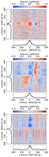 |
Fig. A.1. He I D3 vs Hα(top), Ca II IRT (854.2 nm) vs Hα(middle), and Ca II IRT (854.2 nm) vs He I D3 (bottom) correlation matrices for ESPaDOnS 2016 emission lines. |
Appendix B: Stokes I and V fit from ZDI reconstruction
In this section we show the fit of the LSD profiles by the ZDI reconstruction for the three data sets studied. The Stokes I profiles are shown in Fig. B.1 and the Stokes V profiles in Fig. B.2.
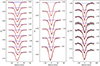 |
Fig. B.1. Fit (red) of the observed (black) Stokes I profiles from the ZDI reconstruction for ESPaDOnS 2016 (left), 2019 (middle) and SPIRou (right) observations. The grey-shaded area corresponds to the uncertainties in the observation, and the number at the right of each profile indicates its rotation cycle. |
Appendix C: BIS versus radial velocity
This appendix presents the analysis of the BIS and radial velocity correlation. These results are discussed in Sect. 4.
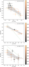 |
Fig. C.1. BIS vs RV of ESPaDOnS 2016 (top), 2019 (middle), and SPIRou (bottom) observations. The colour code scales the HJD of observations. The red dotted line shows the best linear regression with slope "a" and intercept "b" indicated in legend. The uncertainty on the regression is shown as the grey-shaded area The green dotted line has a slope of −1 and an intercept equal to the mean radial velocity. |
All Tables
Magnetospheric truncation radius obtained using the various magnetic field measurements.
All Figures
|
Fig. 1. Radial velocity curves determined for the observation summarised in Table 1. Top: Radial velocity vs. HJD. The vertical dotted line marks the switch from ESPaDOnS to SPIRou, and the different colours represent different rotation cycles. Bottom: Same as above, but folded in phase with P = 7.417 d and T0 = 2 457 544.40981. The dotted curve shows the sinus fit. |
| In the text | |
|
Fig. 2. Variability of 2016 Balmer lines of EX Lup. Top row: Hα(left), Hβ(middle), and Hγ(right) residual lines profiles. Each colour represents a different observation. Bottom row: 2D periodograms of the Hα(left), Hβ(middle), and Hγ(right) residual lines. The dotted white line marks the rotation period of 7.417 d. |
| In the text | |
|
Fig. 3. Variability of the 2019 Balmer lines of EX Lup. Top row: Hα(left), Hβ(middle), and Hγ(right) residual lines profiles. Each colour represents a different observation. Bottom row: Hα(left), Hβ(middle), and Hγ(right) residual line auto-correlation matrices. The colour-code scales the correlation coefficient. Light yellow represents a strong correlation, and dark purple shows a strong anti-correlation. The strong anti-correlation around +350 km s−1 in the Hβ and Hγ matrices is probably an artefact because it is located in a part of the continuum that varies very little. |
| In the text | |
|
Fig. 4. EX Lup He I D3 line variability. Top row: 2016 (left) and 2019 (right) line profiles. Bottom row: Auto-correlation matrices of the 2016 (left) and 2019 (right) lines. |
| In the text | |
|
Fig. 5. He I D3 2016 2D periodogram. |
| In the text | |
|
Fig. 6. Radial velocity fit of He I D3 2016 NC (top) and its version folded in phase (bottom) following the ephemeris given in Eq. (1). |
| In the text | |
|
Fig. 7. ESPaDOnS 2016 Ca II IRT (854.2 nm) residual line profiles (left), 2D periodogram (middle), and auto-correlation matrix (right). |
| In the text | |
|
Fig. 8. ESPaDOnS 2019 Ca II IRT (854.2 nm) residual line profiles (top) and auto-correlation matrix (bottom). |
| In the text | |
|
Fig. 9. SPIRou He I (1083 nm) line profiles (left), 2D periodogram (middle), and auto-correlation matrix (right). |
| In the text | |
|
Fig. 10. ESPaDOnS 2016 LSD Stokes I(left) and V(right) profiles. The rotation phase and the HJD are indicated left and right of each profile, respectively. The scale is indicated in the bottom left corner of each plot. |
| In the text | |
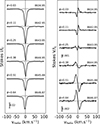 |
Fig. 11. Same as Fig. 10, but for the ESPaDOnS 2019 observations. |
| In the text | |
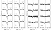 |
Fig. 12. Same as Fig. 10, but for the SPIRou observations. |
| In the text | |
|
Fig. 13. Bℓ curves from LSD profile (top two panels) and from He I D3 line (bottom two panels). |
| In the text | |
|
Fig. 14. Brightness maps from the ESPaDOnS 2016, 2019, and SPIRou data sets (left, middle, and right, respectively) on a flattened polar view. The central dot is thus the pole, the two dotted circles are latitude 60 and 30°, and the solid circle represents the equator. The black ticks show the clockwise rotation phases, and the red ticks represent the observed phases. The colour-code indicates the brightness on a linear scale, where a value of 1.0 represents the quiet photosphere. Values lower than one are darker regions, and values greater than one are bright. |
| In the text | |
|
Fig. 15. Radial (top row), azimuthal (middle row), and meridional (bottom row) magnetic maps from the ESPaDOnS 2016, 2019, and SPIRou data sets (left, middle, and right columns, respectively) in the same flattened polar view as Fig. 14. The colour-code scales the magnetic field strength from dark blue for the strongest negative value to dark red for the strongest positive value. |
| In the text | |
|
Fig. 16. Results of the ESPaDOnS Zeeman intensification analysis. Top: Distribution of the average magnetic field of EX Lup for the 2016 (left) and 2019 (right) data sets. The solid red line represents the median, and the dashed lines represent the 68 % confidence regions. Bottom: Fit to 2016 (left) and 2019 (right) optical Ti I multiplet of EX Lup. The solid red line shows the best fit to the observations in black, while the dashed blue line shows the non-magnetic spectra with otherwise identical stellar parameters. The shaded area marks the region used for the fit. |
| In the text | |
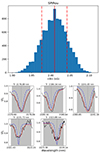 |
Fig. 17. Same as Fig. 16, but for the SPIRou IR Ti I multiplet. |
| In the text | |
|
Fig. A.1. He I D3 vs Hα(top), Ca II IRT (854.2 nm) vs Hα(middle), and Ca II IRT (854.2 nm) vs He I D3 (bottom) correlation matrices for ESPaDOnS 2016 emission lines. |
| In the text | |
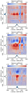 |
Fig. A.2. Same as Fig. A.1 but for ESPaDOnS 2019 emission lines. |
| In the text | |
|
Fig. B.1. Fit (red) of the observed (black) Stokes I profiles from the ZDI reconstruction for ESPaDOnS 2016 (left), 2019 (middle) and SPIRou (right) observations. The grey-shaded area corresponds to the uncertainties in the observation, and the number at the right of each profile indicates its rotation cycle. |
| In the text | |
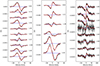 |
Fig. B.2. Same as Fig. B.1 but for Stokes V profiles. |
| In the text | |
|
Fig. C.1. BIS vs RV of ESPaDOnS 2016 (top), 2019 (middle), and SPIRou (bottom) observations. The colour code scales the HJD of observations. The red dotted line shows the best linear regression with slope "a" and intercept "b" indicated in legend. The uncertainty on the regression is shown as the grey-shaded area The green dotted line has a slope of −1 and an intercept equal to the mean radial velocity. |
| In the text | |
Current usage metrics show cumulative count of Article Views (full-text article views including HTML views, PDF and ePub downloads, according to the available data) and Abstracts Views on Vision4Press platform.
Data correspond to usage on the plateform after 2015. The current usage metrics is available 48-96 hours after online publication and is updated daily on week days.
Initial download of the metrics may take a while.