| Issue |
A&A
Volume 670, February 2023
|
|
|---|---|---|
| Article Number | A165 | |
| Number of page(s) | 18 | |
| Section | Stellar structure and evolution | |
| DOI | https://doi.org/10.1051/0004-6361/202245194 | |
| Published online | 21 February 2023 | |
Misalignment of the outer disk of DK Tau and a first look at its magnetic field using spectropolarimetry
1
Dublin Institute for Advanced Studies, Astronomy & Astrophysics Section, 31 Fitzwilliam Place, Dublin 2, Ireland
e-mail: This email address is being protected from spambots. You need JavaScript enabled to view it.
2
Tartu Observatory, University of Tartu, Observatooriumi 1, Tõravere, 61602 Tartumaa, Estonia
3
University of Western Ontario, Department of Physics & Astronomy, London, Ontario N6A 3K7, Canada
4
Leiden Observatory, Leiden University, PO Box 9513 2300 RA Leiden, The Netherlands
5
Univ. Grenoble Alpes, CNRS, IPAG, 38000 Grenoble, France
6
LUPM, Université de Montpellier & CNRS, 34095 Montpellier Cedex 05, France
7
Univ. de Toulouse, CNRS, IRAP, 14 Avenue Belin, 31400 Toulouse, France
Received:
12
October
2022
Accepted:
22
December
2022
Abstract
Context. Misalignments between a forming star’s rotation axis and its outer disk axis, although not predicted by standard theories of stellar formation, have been observed in several classical T Tauri stars (cTTs). The low-mass cTTs DK Tau is suspected of being among them. In addition, it is an excellent subject to investigate the interaction between stellar magnetic fields and material accreting from the circumstellar disk, as it presents clear signatures of accretion.
Aims. The goal of this paper is to study DK Tau’s average line-of-sight magnetic field in both photospheric absorption lines and emission lines linked to accretion, using spectropolarimetric observations, as well as to examine inconsistencies regarding its rotation axis.
Methods. We used data collected with the ESPaDOnS spectropolarimeter, at the Canada-France-Hawaii Telescope, and the NARVAL spectropolarimeter, at the Télescope Bernard Lyot, probing two distinct epochs (December 2010 to January 2011 and November to December 2012), each set spanning a few stellar rotation cycles. We first determined the stellar parameters of DK Tau, such as effective temperature and vsini. Next, we removed the effect of veiling from the spectra, then obtained least-squares deconvolution (LSD) profiles of the photospheric absorption lines for each observation, before determining the average line-of-sight magnetic field from them. We also investigated accretion-powered emission lines, namely the 587.6 nm HeI line and the CaII infrared triplet (at 849.8 nm, 854.2 nm and 866.2 nm), as tracers of the magnetic fields present in the accretion shocks.
Results. We find that DK Tau experiences accretion onto a magnetic pole at an angle of ∼30° from the pole of its rotation axis, with a positive field at the base of the accretion funnels. In 2010 we find a magnetic field of up to 0.95 kG (from the CaII infrared triplet) and 1.77 kG (from the HeI line) and in 2012 we find up to 1.15 kG (from the CaII infrared triplet) and 1.99 kG (from the HeI line). Additionally, using our derived values of period, vsini and stellar radius, we find a value of 58° (+18)(−11) for the inclination of the stellar rotation axis, which is significantly different from the outer disk axis inclination of 21° given in the literature.
Conclusion. We find that DK Tau’s outer disk axis is likely misaligned compared to its rotation axis by 37°.
Key words: stars: individual: DK Tau / stars: variables: T Tauri, Herbig Ae/Be / stars: magnetic field / accretion, accretion disks / techniques: polarimetric / techniques: spectroscopic
© The Authors 2023
 Open Access article, published by EDP Sciences, under the terms of the Creative Commons Attribution License (https://creativecommons.org/licenses/by/4.0), which permits unrestricted use, distribution, and reproduction in any medium, provided the original work is properly cited.
This article is published in open access under the Subscribe to Open model. This email address is being protected from spambots. You need JavaScript enabled to view it. to support open access publication.
1. Introduction
Stellar magnetic fields are omnipresent and play an essential role in the formation of stars and planets. Understanding their impact is therefore crucial to the study of stellar birth. We do not, however, yet possess a complete picture of how stellar magnetic fields originate, how they evolve over time, or the extent of their impact on circumstellar disks and the accretion process in the early stages of a star’s life (see e.g., Bouvier et al. 2007; Gregory et al. 2012; Folsom et al. 2016; Hartmann et al. 2016; Villebrun et al. 2019). Stellar magnetic fields of accreting T Tauri stars play an essential role in driving accretion and strongly impact the geometry of the accretion flow (see Hartmann et al. 2016). By analyzing the magnetic field along the line-of-sight and integrated over the visible stellar hemisphere measured in the acc retion-powered emission lines, one can recreate a picture of the component of the stellar magnetic field that dominates the accretion process. This is an integral quantity that relates Stokes I and Stokes V, making use of spectropolarimetric data. The interested reader is referred to, for example, Rees & Semel (1979), Donati & Landstreet (2009), Morin (2012). The Stokes parameters and the magnetic field are connected through the Zeeman effect. This effect describes the impact of a magnetic field on a spectrum: its atomic (and molecular) lines are broadened or split, depending on the strength of the field and the sensitivity of the line in question (see e.g., Tennyson 2011; Hussain & Alecian 2014).
In this work, we analyze the spectropolarimetry of the classical T Tauri star (cTTs) DK Tau. DK Tau is a young low-mass star surrounded by a circumstellar disk which is actively accreting from its inner regions. It is a wide binary (separation  , equivalent to 307 au – see e.g., Manara et al. 2019), which allows DK Tau A (hereafter “DK Tau”) to be spatially resolved with spectropolarimetry and studied on its own. It is located in the Taurus Molecular Cloud at a distance of 132.6 pc Gaia Collaboration (2016, 2018, 2023). Its spectral type is K7 (see e.g., Johns-Krull 2007; Fischer et al. 2011) with a heliocentric radial velocity of +16.2 km s−1 (Kounkel et al. 2019). Rota et al. (2022) measured the inclination, with respect to the line of sight, of its outer (> 20 au) gaseous disk axis via projection to be 21°, using the 12CO (J = 2 − 1) line with ALMA. The star’s rotation period P, as determined using photometry, has been measured as 8.4 days Bouvier et al. (1993) and 8.18 days Percy et al. (2010), Artemenko et al. (2012).
DK Tau presents with significant and variable veiling (a strong signature of accretion – see e.g., Hartigan et al. 1995; Fischer et al. 2011). In addition to accretion, it also shows evidence of ejection (see e.g., Hartigan et al. 1995), in particular inner disk winds and a jet as revealed by the detection of both low and high velocity forbidden [OI] emission by Hartigan et al. (1995) and Banzatti et al. (2019).
The effect of veiling on spectra complicates magnetic field measurements, yet the study of active accretors is very valuable for understanding the interaction between stellar magnetic fields and accreting material from the circumstellar disk. Indeed, our current understanding of magnetospheric accretion (see e.g., Shu et al. 1994; Romanova et al. 2002; Bessolaz et al. 2008; Hartmann et al. 2016) involves the truncation of the inner circumstellar disk at a few stellar radii and the channeling of accretion in funnel flows by the stellar magnetic field. When the accreted matter falls onto the star at near free-fall velocities, it produces an accretion shock close to the stellar surface, which gives rise to continuum and line veiling Calvet & Gullbring (1998) and generates a localized bright/hot spot at the level of the chromosphere.
Simple models of stellar formation do not account for a misalignment between the star’s rotation axis and its outer disk axis. However, misalignments may be common, as several dippers display a low inclination of their outer disk axis (see e.g., Ansdell et al. 2020; Sicilia-Aguilar et al. 2020). Dippers are stars that show flux dips in their light curves. The standard explanation involves circumstellar material from the inner disk passing in front of the star, occulting it periodically or aperiodically (see e.g., McGinnis et al. 2015; Roggero et al. 2021). Dippers therefore require a relatively high inclination for the inner disk axis (which is here assumed to point in the same direction as the stellar rotation axis), that is inconsistent with their measured outer disk axis inclination. Such a misalignment has been directly measured in few cTTs (see e.g., Alencar et al. 2018; Bouvier et al. 2020). These observations suggest a more complex formation mechanism than normally considered, though it is not clear what gives rise to such a misalignment. As examples of potential causes, Sicilia-Aguilar et al. (2020) suggest the possibility of two different protostellar collapses, whereas Alencar et al. (2018) invoke the presence of a massive planet inside the disk gap, and Benisty et al. (2018) the effects of a low-mass stellar companion. DK Tau shows signs of being one of these systems with a misaligned outer disk.
In this paper, we describe our observations in Sect. 2. We detail our analysis and results regarding stellar parameters, veiling, and magnetic characterizations in Sect. 3. In Sect. 4 we discuss the implications of the inclination we measure for DK Tau and its magnetic field. Finally, Sect. 5 contains our conclusions.
2. Observations
Our data set is comprised of two sets of circularly polarized spectra of DK Tau, collected from December 2010 to January 2011, and from the end of November to the end of December 2012, with the spectropolarimeters ESPaDOnS (Echelle SpectroPolarimetric Device for the Observation of Stars), mounted at the CFHT (Canada-France-Hawaii Telescope) 3.6 m telescope in Hawaii (Donati et al. 2006), and NARVAL, mounted at the 2 m TBL (Télescope Bernard Lyot) on the Pic du Midi in France (Aurière 2003). These echelle spectropolarimeters cover the visible domain, from 370 to 1050 nm, in a single exposure, and have a resolving power of 65 000. ESPaDOnS has a fiber aperture of  , while NARVAL has one of
  .
.
Table 1 lists the dates of the middle of the observations for the two ESPaDOnS and NARVAL data sets. The total exposure time was 4996.0 s for each ESPaDOnS observation and 4800.0 s for each NARVAL observation. In 2010 a total of 15 observations were taken over 39 days, and in 2012 a total of 12 observations were taken over 35 days, with the intention of capturing a few rotation cycles of the target in each set.
Dates for the 2010 and 2012 ESPaDOnS and NARVAL data sets.
The data are public and were downloaded from the archive of the PolarBase website1 (see e.g., Petit et al. 2014). These observations were made as a result of proposals 10BP12 and 12BP12, with J.-F. Donati as P.I. in both cases and obtained as part of the MaPP (Magnetic Protostars and Planets) large program at the CFHT. We also downloaded the corresponding image files for the ESPaDOnS data from the Canadian Astronomy Data Centre (CADC) website2. The data had been previously reduced at the CFHT and TBL. The reduction was carried out with the LibreESpRIT (for “Echelle Spectra Reduction: an Interactive Tool”) reduction package specifically built for extracting polarization echelle spectra from raw data. This includes subtracting the bias and the dark frames, and correcting for the variations in sensitivity using flat field frames (Donati et al. 1997). The spectra were continuum normalized in addition to the LibreESpRIT automatic continuum normalization, as the automatic procedure is not tailored for stars presenting with emission lines and it did not manage to properly adjust the continuum.
3. Analysis and results
3.1. Veiling
Accretion shocks are at a higher temperature than the photosphere. This adds an extra continuum to the stellar continuum, artificially decreasing the depth of the photospheric absorption lines. This is known as veiling and it varies with the wavelength, and can also vary from night to night. Its effect needs to be removed from the spectra in order to analyze the stellar magnetic field from the photospheric absorption lines.
Veiling (R) is defined as the ratio between the flux of the accretion shock and the photospheric flux. For a normalized spectrum, it can be expressed using the following equation:
![Mathematical equation: $$ \begin{aligned} I_{\mathrm{v} }(\lambda ) = [I_{\mathrm{ph} }(\lambda ) + R(\lambda )] N(\lambda ) \end{aligned} $$](/articles/aa/full_html/2023/02/aa45194-22/aa45194-22-eq4.gif) (1)
(1)
where Iv(λ) refers to the veiled intensity at wavelength λ, Iph(λ) to the intensity of the photosphere at wavelength λ, R(λ) to the veiling at wavelength λ and N(λ) is a normalization constant at wavelength λ.
In order to measure the veiling in our spectra, we used a technique based on the fitting of a rotationally broadened and artificially veiled weak-lined T Tauri star (wTTs) spectrum to the spectrum of DK Tau. By choosing a wTTs with the same spectral type as our cTTs and coming from the same star forming region3, this wTTs can be seen as the purely photospheric version of our star because it experiences no accretion. We tested several wTTs with a K7 spectral type and a line-of-sight-projected equatorial rotational velocity vsini lower than the vsini of DK Tau (see Sect. 3.2), in order to find the one that provided the best fit. We ultimately used the spectrum of TAP45 (which has a vsini of 11.5 km s−1 – see Feigelson et al. 1987; Bouvier et al. 1993) as a template to estimate the veiling across DK Tau’s spectra as the extra continuum that has to be added to the wTTs spectrum in order to reproduce the veiled cTTs spectrum (at the lowest χ2 level).
We obtained values of the veiling as a function of the wavelength (in bins of ∼20 nm), for each spectrum. When the value is less than ∼0.4 throughout the spectrum, we see that it is approximately constant in wavelength, therefore we took the mean value as R for the whole spectrum. When it is larger than this, we fit a linear relation through the points and considered this function as our R(λ). We then inverted Eq. (1) to recover the normalized photospheric spectrum of each observation. Figure 1 shows the night with the least veiling and the one with the most veiling on the top and bottom panel respectively.
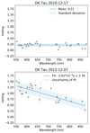 |
Fig. 1. Veiling (gray dots), the best linear fit (blue line) and the standard deviation (light blue shaded region) as a function of wavelength for the fourth night of the 2010 ESPaDOnS observations (top panel) and for the seventh night of the 2012 ESPaDOnS observations (bottom panel). |
In 2010, the peak values of veiling (at ∼550 nm) for each observation range from 0.2 to 1.8. Three observations out of fifteen have nearly constant veiling values across their spectrum. In 2012, the peak values of veiling for each observation range from 0.2 to 1.3 (lower than the value from two years before). Only one observation out of twelve has a nearly constant veiling value across its spectrum.
For the two sets of observations, we see that the slope of veiling as a function of wavelength steepens when the veiling is higher as well. We also find that when the veiling is high, there is more scatter. We believe this scatter is due to the correlation of stronger line emission with stronger mass accretion rate (see e.g., Dodin & Lamzin 2012; Rei et al. 2018). In that case, individual line emission would contribute more to the veiling by filling in absorption lines; whereas for nights when the veiling is low, continuum veiling would remain the dominant form of veiling. The interpretation of these trends goes beyond the scope of this work, and will be investigated in a subsequent paper.
3.2. Stellar parameters
Given the importance of accurate stellar parameters, we took advantage of ESPaDOnS and NARVAL’s continuum normalized high resolution spectra to derive precise values for DK Tau, in particular of the line-of-sight-projected equatorial rotational velocity vsini, needed to investigate the potential misalignment of DK Tau’s outer disk, and for the effective temperature Teff, which is needed for our analysis. For this, we first obtained the mean spectrum of the four nights with the least amount of veiling (i.e., R = 0.2 for all four nights, see Sect. 3.1) in order to get a spectrum with a higher signal to noise ratio of 136, whereas the individual spectra had a signal to noise ratio of 103 on average. We then used the ZEEMAN spectrum synthesis program, developed by Landstreet (1988) and Wade et al. (2001) and modified by Folsom et al. (2016) to derive the stellar parameters. Under the assumption of local thermodynamic equilibrium, this code solves radiative transfer equations. It iteratively compares a synthetic spectrum (calculated using a grid of model atmospheres and a list of atomic data) with the observation, by χ2 minimization, to determine free model parameters. Veiling was included in the model.
We used the Vienna Atomic Line Database (VALD) website4 (see e.g., Ryabchikova et al. 2015) to acquire a continuous atomic line list ranging from 400 nm to 1000 nm for a star of Teff = 4000 K, logarithmic surface gravity log g = 4 (in cgs units) and a solar metallicity. We used the MARCS model atmosphere grid of Gustafsson et al. (2008). In the ZEEMAN code, we specified the following initial values for the stellar parameters: for Teff and vsini, we used the values provided in the literature, of Teff = 4000 K Herczeg & Hillenbrand (2014), and vsini = 12.7 km s−1 McGinnis et al. (2020). We used log g = 4 (in cgs units), as this is typical of T Tauri stars (TTs), microturbulence velocity vmic = 1 km s−1, macroturbulence velocity vmac = 0 km s−1, solar metallicity and a veiling of 0.1. We started with a model with initial values of Teff, vsini, log g and veiling for a fixed value of vmic, vmac and metallicity. We then ran fits with only Teff and vsini as free parameters. When fitting the observation, we used a wavelength range from 400 nm to 1000 nm. We ran the code on several windows throughout the spectrum. We calculated the average of the values obtained for the different spectral windows and took the standard deviation of the spread as the error bars. We derive a Teff of 4150 ± 110 K and a vsini of 13.0 ± 1.3 km s−1. We note that our values are in good agreement with the ones found in the literature (see Herczeg & Hillenbrand 2014; McGinnis et al. 2020).
We also determined DK Tau’s radius. We first calculated the stellar luminosity L⋆ using the J-band magnitudes of Eisner et al. (2007). As DK Tau A and B are not spatially resolved in their observations, we corrected the J-band magnitude to remove the contribution of DK Tau B. This was done by extrapolating the brightness ratio given by Eisner et al. (2007) for the K-band (of 3.3) to the J-band, taking into consideration the shape of the continua of the two stars based on their respective spectral types, as well as the individual extinction each star suffers (i.e., AV = 0.7 mag for DK Tau A, and AV = 1.80 mag for DK Tau B – Herczeg & Hillenbrand 2014). We find a flux ratio of 4.4 for the J-band. We then corrected the magnitude for the extinction in DK Tau A (i.e., 0.7 mag) Herczeg & Hillenbrand (2014)
5. It can be noted that the value for the extinction quoted by Fischer et al. (2011) is a factor 2 higher. The variability of the extinction is probably connected to the dipper behavior of the star (Roggero et al. 2021). We also corrected for a veiling of RJ = 0.3 ± 0.1, based on an interpolation of our measurements of veiling as a function of wavelength (see Sect. 3.1). This is very similar to the values observed by Fischer et al. (2011). We then used the bolometric correction in the J band from Pecaut & Mamajek (2013). We find a value of L⋆ = (1.65 ± 0.25) L⊙. Using the relation  and our measured value of Teff, we derive a stellar radius of R⋆ = (2.48 ± 0.25) R⊙.
Table 2 summarizes the measured properties of DK Tau. The inclination of the outer disk axis was measured by Rota et al. (2022) using ALMA observations. We derive a different value for the inclination i of the stellar rotation axis (see Sect. 4.1). The stellar rotation period P mentioned in the literature is based on photometry (see Bouvier et al. 1993; Percy et al. 2010; Artemenko et al. 2012). The mass M⋆ was derived by Johns-Krull (2007) from pre-main sequence evolutionary tracks. Using the Siess et al. (2000) models6, we find that the values of Teff and L⋆ that we obtain give a slightly higher M⋆ than the one of 0.7 M⊙ derived by Johns-Krull (2007), but it agrees with 0.7 M⊙ within 2σ (see Appendix A).
Summary of the measured properties of DK Tau.
3.3. Least-squares deconvolution
Least-squares deconvolution (LSD) is a cross-correlation technique used to add the signatures from hundreds of photospheric absorption lines and obtain an average line profile of very high signal to noise ratio (see e.g., Donati et al. 1997; Kochukhov et al. 2010). It makes use of a line mask, a list describing the position and depth of the chosen absorption lines. We first created a line mask using the VALD line list (with a detection threshold of 0.01, Teff = 4000 K, log g = 4 and vmic = 1 km s−1) and assuming an ATLAS9 stellar atmosphere model (Kurucz 1993). Next, using our line mask, we applied LSD to all observations in the range from 500 nm to 1000 nm (i.e., excluding the blue edge of the spectra because of excess noise), excluding regions with telluric and emission lines, as well as the lines most affected by accretion7, in order to obtain a mean line profile for each veiling-corrected spectrum. We set the effective Landé factor ḡ0 = 1.4, the central intensity d0 = 0.47 and the equivalent wavelength λ0 = 650.0 nm for all the nights (see Kochukhov et al. 2010). The LSD profiles were then normalized to be at the same equivalent width. The latter was done in order to correct for the residual effects of veiling. For all nights, we obtained a definite Zeeman signal detection in the LSD profiles, with a false alarm probability smaller than 0.001% (see the LSD profiles in Appendix B).
The Stokes I LSD profiles of the ESPaDOnS and NARVAL observations made on 19 December 2010 presented a small absorption feature blueward of the main absorption line (see e.g., Fig. 2). The other nights all showed a single photospheric absorption line. This small absorption feature is due to scattered moonlight, as the full Moon was close to DK Tau on that night (with an angular separation of about 8°), and as the contamination is at the expected lunar radial velocity in the heliocentric rest frame8. This type of contamination has been seen before (see e.g., Donati et al. 2011).
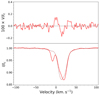 |
Fig. 2. LSD profile (in the heliocentric velocity frame) of Stokes V (top) and Stokes I (bottom) parameters normalized to the continuum for the sixth night of the 2010 ESPaDOnS observations. Note on this night scattered light from the Moon caused the small blue-ward absorption feature. For comparison, we also show the seventh night of the 2010 ESPaDOnS observations (dashed line), which did not suffer from moonlight contamination. |
We fit the wing of the main absorption feature with that of a Voigt profile and manually removed the contamination.
3.4. Average line-of-sight magnetic field
We measured the magnetic field along the line-of-sight and integrated over the visible stellar hemisphere, Blos 9, by using Eq. (3.3) from Morin (2012):
![Mathematical equation: $$ \begin{aligned} B_{\mathrm{los} }(G) = -2.14 \times 10^{11} \frac{\int {v \, V(v) \, \mathrm{d}v}}{\lambda _{0} \, g_{\mathrm{eff} } \, c \, \int {[I_{\rm c} - I_{v}] \, \mathrm{d}v}} \end{aligned} $$](/articles/aa/full_html/2023/02/aa45194-22/aa45194-22-eq6.gif) (2)
(2)
on the LSD profiles of the photospheric absorption lines (see also Rees & Semel 1979; Donati et al. 1997; Wade et al. 2000). In this equation, v is the radial velocity in the rest frame of the star, V refers to Stokes V, λ0 is the wavelength of the line center in nm, geff is the effective Landé factor of the line, I refers to Stokes I and Ic to the unpolarized continuum. We find values ranging from −0.19 ± 0.05 kG to 0.20 ± 0.03 kG in 2010 and from −0.13 ± 0.02 kG to 0.08 ± 0.02 kG in 2012 (see Fig. 3, and see the list of values in Appendix B). It should be noted that, since Blos represents a signed average over the visible stellar hemisphere, regions of opposite polarities partly cancel out.
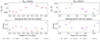 |
Fig. 3. Average line-of-sight magnetic field Blos as derived from the photospheric absorption lines and veiling over time, shown folded in phase with the derived 8.2 day period, for the 2010 (left panel) and 2012 (right panel) datasets. Different colors and symbols represent different rotation cycles. |
We applied a phase dispersion minimization (PDM; Stellingwerf 1978) technique on the 2010 Blos values and found a period of 8.20 ± 0.13 days. Since this is the period of the modulation of the stellar magnetic field, it accurately represents the stellar rotation period. This period is consistent with values found in the literature from photometry (8.4 days from Bouvier et al. 1993, and 8.18 days from Percy et al. 2010; Artemenko et al. 2012). Small discrepancies could be explained by differential rotation: different measurements tracking features at various latitudes.
3.5. Emission lines
After analyzing the LSD profiles of photospheric absorption lines to derive the associated Blos linked to non-accreting regions, we also investigated emission lines associated with accretion shocks, in particular the narrow component of the 587.6 nm HeI line and of the CaII infrared triplet (IRT – at 849.8 nm, 854.2 nm and 866.2 nm). They can be used to get more information on DK Tau’s magnetic fields, as they are tracers of the fields present at the footpoints of accretion funnels (see e.g., Donati et al. 2007). These lines are known to have multiple components (see e.g., Beristain et al. 2001; McGinnis et al. 2020), often containing a narrow component (NC), originating from the accretion shock, and a much broader component (or components), which likely forms farther out in the accretion columns or in hot winds. For this reason, we decomposed the profiles using a fit of 2 or more Gaussians in order to isolate the NC (examples of these fits can be seen in Appendix C). For the CaII lines, we then averaged the three lines into a single LSD-like profile in order to increase the signal to noise ratio, as it has been done in other studies (see e.g., Donati et al. 2007, 2008, 2012. Since this is a triplet, the shape of all three lines should be the same (see e.g., Azevedo et al. 2006). In addition, in our data, we see an intensity ratio close to 1:1:1 and the NCs are not contaminated by the nearby Paschen emission lines at 850.2 nm, 854.5 nm and 866.5 nm. The NC of the HeI line is believed to be generated in the post-shock region at the base of the magnetic accretion funnels that connect the surface of the star to its inner disk. The NC of the CaII IRT is thought to probe the accretion regions and the chromosphere.
The Stokes V and Stokes I profiles of the HeI emission line and the CaII IRT, for both epochs, can be seen in Fig. 4. The Stokes V profiles of the emission lines show similar signatures with phase. This indicates that the accretion spot is mostly likely located at a high enough latitude to be visible with the same polarity at all times. They also indicate that the field is positive (i.e., pointing toward the observer) at the base of the accretion funnels that connect the star to its circumstellar disk.
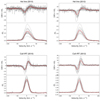 |
Fig. 4. Stokes V and Stokes I profiles (in gray) and average (in red) of the HeI emission line (top panels) and the CaII IRT (bottom panels), for the 2010 (left panels) and 2012 (right panels) observations. |
We measured Blos in the emission lines using the same method as described in Sect. 3.4. We find values ranging from 0.20 ± 0.51 kG to 1.77 ± 0.08 kG for HeI in 2010, from 0.48 ± 0.09 kG to 1.99 ± 0.09 kG for He I in 2012, from 0.34 ± 0.04 kG to 0.95 ± 0.02 kG for CaII in 2010, from 0.26 ± 0.02 kG to 1.41 ± 0.05 kG for CaII in 2012. Figure 5 shows the obtained values folded in phase (and the list of values can be found in Appendix C). The values of Blos are higher in 2012. We find that the values measured through the CaII IRT are lower than the ones measured through the HeI line. It has been hypothesized that the lower intensity of Blos found using the CaII IRT stems from the dilution of the emission from the accretion shock by chromospheric emission (see e.g., Donati et al. 2019), which results in the Stokes V/I profile being shallower for the CaII IRT than for the HeI line.
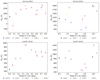 |
Fig. 5. Average line-of-sight magnetic field Blos over time, shown folded in phase with an 8.2 day period, for the HeI emission line (top panels) and the Ca II IRT (bottom panels), for the 2010 (left panel) and 2012 (right panel) datasets. Different colors and symbols represent different rotation cycles. |
We find extreme values of Blos in the emission lines that are one order of magnitude larger than the extreme values of Blos derived from the LSD profiles of the photospheric absorption lines (see Fig. 3), showing strong fields in the accretion shocks. This is consistent with the current understanding of accretion shocks as compact regions with some of the strongest magnetic field concentrating in dark polar regions at the surface of the star and magnetic field lines reaching to the circumstellar disk. For both epochs, we only see the positive pole and never the negative one.
The plots of the Blos in the emission lines in 2012 do not fold well in phase. We believe this may stem from the location of the accretion shocks being more dynamic and/or the accretion being more complex, with more than one accretion shock. This is also observed in the variability of veiling in 2012 (see Fig. 3), which does not fold well with the rotation phase, indicating that there is considerable intrinsic variability in the mass accretion rate.
We derived the equivalent width (EW) of the HeI emission line. Figure 6 shows the obtained values folded in phase (and the list of values can be found in Appendix C). When the EW is larger, we are seeing more of the accretion shock in our line-of-sight. This is also when we measure stronger magnetic fields using emission lines tracing the accretion shock (see Fig. 5), as expected following the paradigm of magnetospheric accretion.
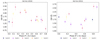 |
Fig. 6. Equivalent width (in Å) of the HeI emission line over time, shown folded in phase with an 8.2 day period, for the 2010 (left panel) and 2012 (right panel) datasets. Different colors and symbols represent different rotation cycles. |
3.6. Magnetic obliquity
We used the third equation of Preston (1967), which assumes a pure dipole, a simplification of the magnetic field present in the accretion shocks, to calculate an estimate of the magnetic obliquity (i.e., the angle between the stellar rotation axis and the magnetic field axis) derived from the emission lines. We used the extreme values found for Blos in the emission lines and an inclination i of 58°. For the HeI emission line, we find a magnetic obliquity10 of 26° for the 2010 epoch, and of 21° for the 2012 epoch. For the CaII IRT, we find a magnetic obliquity of 16° for the 2010 epoch, and of 23° for the 2012 epoch. These estimates are consistent with the Stokes V signatures of the emission lines. They are also consistent with the magnetic obliquity of 18° (+8)(−7) in 2011 derived by McGinnis et al. (2020), using the radial velocity variability of the HeI emission line and assuming one accretion spot. We therefore have an agreement between the values derived from the magnetic field that drives the accretion and the value derived from a result of accretion.
The estimates of the magnetic obliquity are consistent with only seeing the positive pole in the plots of the Blos in the emission lines, confirming that DK Tau experiences nearly poleward accretion, with a positive field at the base of the accretion funnels.
The HeI emission lines show a radial velocity variability with a small amplitude, which is another indication that the accretion spot is most likely close to the pole. As the star rotates, if the accretion spot were located at the equator, the velocity variation would be large as the spot gets red and blueshifted.
3.7. Truncation and co-rotation radii
In order to calculate the truncation radius, we need to know the star’s mass accretion rate. For this, we measured the equivalent width (EW) of several emission lines (i.e., Hα, Hβ, Hγ, the HeI lines at 447.1 nm, 667.8 nm and 706.5 nm, as well as the CaII IRT at 849.8 nm, 854.2 nm and 866.2 nm). Since ESPaDOnS and NARVAL’s spectra are not flux calibrated, we created a template for DK Tau based on SO879, a weak-lined T Tauri star with a K7 spectral type (described in Stelzer et al. 2013). The template was corrected for extinction, then scaled to have the same luminosity (i.e., 1.65 L⊙) and be at the same distance (i.e., 132.6 pc) as DK Tau. After correcting the EW for veiling, we used this template to flux calibrate them through the following formula:
 (3)
(3)
where Fline is the flux of the line, EWline is the veiling corrected EW of the line and Fcont is the flux of the continuum of the template at the wavelength of the line in question. Then we obtained the luminosity in each line. Next, we used the relations in Table B.1. from Alcalá et al. (2017) to calculate the accretion luminosity from each line and averaged these values for each night. We then took the average over all nights in each epoch as the accretion luminosity, and the standard deviation of the spread in the values found from different nights as the error bars. We find Lacc = 0.26 ± 0.18 L⊙ in 2010 and Lacc = 0.49 ± 0.42 L⊙ in 2012. These values are similar to the ones found e.g., by Fischer et al. (2011) (i.e., 0.17 L⊙) or by Fang et al. (2018) (i.e., 0.16 L⊙).
We then converted the accretion luminosity into mass accretion rate using Eq. (8) from Gullbring et al. (1998) with the values of R⋆ and M⋆ from Table 2 and Rin = 5 R⋆ (as is typically used). We find log (Ṁacc [M⊙ yr−1]) = −7.43 in 2010, and log (Ṁacc [M⊙ yr−1]) = −7.15 in 2012. These values are consistent with the one of −7.42 quoted by Gullbring et al. (1998). Finally, we used Eq. (6) from Bessolaz et al. (2008) to estimate the truncation radius. This equation assumes an axisymmetric dipole, which is a simplification of DK Tau’s magnetic topology. It also uses the dipolar field calculated at the equator as B⋆. Considering the equatorial value is half of the value at the pole, we estimated the latter (see Preston 1967) using the values of Blos in the emission lines11. This is an approximation, as part of the Blos could come from higher order multipoles, in particular from the octupole, rather than the dipole. We find rtrunc ∼ (5.2 ± 1.1) R⋆ for the HeI emission line in 2010, rtrunc ∼ (3.9 ± 0.8) R⋆ for the CaII IRT12 in 2010, rtrunc ∼ (4.7 ± 1.2) R⋆ for the HeI emission line in 2012, and rtrunc ∼ (3.9 ± 1.0) R⋆ for the CaII IRT in 2012. We calculated the co-rotation radius as well, using Kepler’s third law: rco-rot = 6.1 R⋆. We find that the truncation radius values are consistent with the co-rotation radius within the error bars. This implies that DK Tau is unlikely to be in the propeller regime, an unstable accretion regime, as the truncation radius is not farther than the co-rotation radius Romanova et al. (2018). For the 2010 epoch, DK Tau may be in the stable accretion accretion regime, since the Blos and accretion tracers seem fairly periodic. The truncation radius being slightly smaller than the co-rotation radius is consistent with this as well Blinova et al. (2016).
4. Discussion
4.1. Inconsistencies regarding the inclination
Naively one might assume that the inclination angle i of the stellar rotation axis with respect to the line-of-sight is 21° based on the inclination of the outer gaseous disk axis Rota et al. (2022). DK Tau’s lightcurve however classifies the star as a dipper (Roggero et al. 2021). The traditional explanation invokes circumstellar material passing in front of the star and occulting it. If the disk is seen close to edge on, matter lifted above the disk plane could cause these occultations. However, DK Tau’s outer disk is seen nearly pole on Rota et al. (2022), which is inconsistent with this scenario, unless the stellar rotation axis is at a very different angle than that of the outer disk axis.
Furthermore, based on the star’s rotational properties (see Table 2) and using the following relation
 (4)
(4)
we derive a much higher inclination of 58° (+18)(−11). Therefore, if DK Tau is in fact seen nearly pole on, then P, vsini and R⋆ are not consistent with each other. As the stellar radius is the most uncertain of these parameters13, it is possible that it may have been underestimated. However, if we consider that P, vsini and i are accurately determined, then we would need R⋆ = (6 ± 1) R⊙ for this formula to agree, which is unrealistically large for a TTs.
Another possibility is that the period or vsini may be inaccurate. Regarding vsini, the value we derive agrees within error bars with the one measured by McGinnis et al. (2020), despite using two different assessment methods. It is therefore a value that can be trusted. This leaves the stellar rotation period.
In the literature, the stellar rotation period of DK Tau has been measured using photometry with values ranging from 8.18 days (Percy et al. 2010; Artemenko et al. 2012) to 8.4 days (Bouvier et al. 1993). However, since the photometry is dominated by flux dips that might be due to extinction events (Roggero et al. 2021), it is possible that these dips are caused by circumstellar material that is not located at the co-rotation radius. In that case, the measured period would not be the same as the stellar rotation period.
In Sect. 3.4 we derived a period from the rotational modulation of the line-of-sight magnetic field Blos, which should accurately represent the stellar rotation period. In the context of exoplanet search programs, Blos is indeed often considered as the most reliable indicator of stellar rotation period (see e.g., Hébrard et al. 2016). Additionally, the value we find of 8.20 ± 0.13 days is consistent with those found in the literature from photometry. We therefore find that the value for the period can be trusted.
Moreover, this rotation period can be seen in a number of datasets at our disposal. For example, we computed bidimensional periodograms of the intensity of the HeI (at 587.6 nm) emission line, and the Stokes I and Stokes V LSD profiles of the photospheric absorption lines (see Appendix D). The HeI line comes from the accretion shock and should therefore vary with the stellar rotation period. In 2010 we find a period around 8 days for the entire red-shifted part of the HeI line (from 0 to 50 km s−1), however this period is very uncertain. The Stokes V profile also shows a period near 8.5 days between ∼ − 20 and −7 km s−1 and between ∼0 and 8 km s−1, but again the uncertainty is large. The Stokes I profile does not show a clear period. In 2012 there is no clear period found from the HeI line, likely because accretion is more intrinsically variable in this epoch than 2 years prior. Again no clear period is observed from the Stokes I profile, but the Stokes V profile shows a possible periodicity at around 8 days (albeit with a large uncertainty, same as in 2010).
Furthermore, the variation of the 2010 veiling as a function of time is also consistent with an 8.2 day period (see Fig. 3). The variation of the 2012 veiling as a function of time, however, does not seem to follow any trend with the period. This is consistent with the intensity of the He I line not showing a clear correlation with period in this epoch, since both are tracing accretion. This is another indication that there must be some intrinsic variability in the mass accretion rate in 2012, which masks any rotational modulation of the accretion spot(s).
We looked at the possibility of the rotation period or vsini being inaccurate and found evidence to the contrary. Because their values appear to be accurate, we deduce that it is the value for the inclination that is problematic. We conclude that the inclination measured for the outer circumstellar disk axis must not represent the inclination of the rotation axis of the star. This suggests that there is a considerable misalignment between the rotation axis of DK Tau and its outer disk. When we calculate DK Tau’s inclination based on its rotational properties using Eq. (4), we find i = 58° (+18)(−11). This value is based on vsini = (13.0 ± 1.3) km s−1, P = (8.2 ± 0.2) days and R⋆ = (2.48 ± 0.25) R⊙. It follows that the outer disk axis of DK Tau is likely misaligned by 37° with its rotation axis (see Fig. 7).
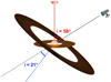 |
Fig. 7. Sketch (not to scale) showing DK Tau in the center, surrounded first by its inner disk, then by its outer disk which is considerably misaligned. The rotation axis at 58° is in red, the outer disk axis at 21° is in blue, and the line-of-sight axis is in gray (by C. Delvaux). |
Misalignments between the inner and outer circumstellar disk axes of T Tauri stars are starting to be observed, when combining near infrared interferometric VLTI/GRAVITY data and millimeter interferometric ALMA data (see e.g., Ansdell et al. 2020; Bouvier et al. 2020), or with shadows observed with VLT/SPHERE (see e.g., Benisty et al. 2018; Sicilia-Aguilar et al. 2020), or with VLTI/GRAVITY (see e.g., Bohn et al. 2022). We find a misalignment between the outer disk axis and the rotation axis. What of the inner disk axis? In young dippers like DK Tau, the material that causes the dips is believed to be located in the inner accretion disk Bouvier et al. (2007), McGinnis et al. (2015), which need to be observed at high inclinations in order for material to cross our line-of-sight to produce the dips. Therefore an inclination of 21° of the inner disk of DK Tau is difficult to reconcile with its dipper light curve. In addition, the inner disk axis is normally expected to be aligned with the stellar rotation axis. We thus find it very likely that the inner disk axis of DK Tau has the same inclination of i = 58° as was calculated for its rotation axis. This inclination is sufficiently high to support the dipper behavior and there are other cases of dippers with similar inclinations (see e.g., McGinnis et al. 2015; Roggero et al. 2021). DK Tau is one more example of a TTS with a misalignment between its inner and outer circumstellar disk axes.
It is also a wide binary system, and the misalignment could stem from the binary formation mechanism: turbulent fragmentation might generate disk axis that are more randomly oriented. It is however interesting to note as well that the outer disk axes of both components of the binary are misaligned by 43° (see Rota et al. 2022), which is close to the value (of 37°) of the misalignment between the inner and outer disk axes of DK Tau A. This could suggest a quasi-alignment of the inner disk axis of DK Tau A with the outer disk axis of DK Tau B, assuming that they are not only aligned compared to our line-of-sight, but that the orientation of their nodes are aligned as well, which is unknown.
4.2. Magnetic field in the accretion-powered emission lines
The Blos derived from the photospheric absorption lines (see Sect. 3.4), gives a partial view of DK Tau’s magnetic fields that exclude the accreting regions, as photospheric absorption lines and accretion-powered emission lines form in different regions of the stellar surface. It is the field present in these accreting regions that is understood to best probe the global stellar magnetic field that reaches to the circumstellar disk. The magnetic obliquity derived from the accretion-powered emission lines is therefore likely to be close to the actual value. We find that the low magnetic obliquity that we derive (see Sect. 3.6), the positive polarity of the Blos in the emission lines, as well as their Stokes V signatures and the range of radial velocity of the HeI line are consistent with the presence of an accretion spot always visible and close to the pole. This is where the accretion funnels connecting DK Tau to its disk would be anchored. This is similar to what has been found for several other cTTs (see e.g., Johnstone et al. 2014; McGinnis et al. 2020).
For the 2010 epoch, we find that the magnetic field in the Ca II IRT (and in the HeI line – see Fig. 5) is at a maximum close to the same phase (i.e., around phase 0.3) as the maximum in the veiling (see Fig. 3), which is when the accretion shock is in our line-of-sight. Around phase 0.5, we see a small redshifted absorption in the Hα line (see Appendix E), indicating that the accretion column is in our line-of-sight, which is directly after the maximum of the magnetic field in the emission lines and the increase in veiling, therefore probably directly after the accretion shock was in our line-of-sight. Because this small redshifted absorption is not perfectly simultaneous with the increase in veiling and in the emission lines, it might be an indication of differential rotation.
5. Conclusions
In this paper, we have studied DK Tau, a low-mass classical T Tauri star (cTTs) with significant veiling (defined as the ratio between the accretion shock flux and the photospheric flux), using dual-epoch spectropolarimetric observations (collected in 2010 and 2012). We derive an effective temperature Teff of 4 150 ± 110 K and a line-of-sight-projected equatorial rotational velocity vsini of 13.0 ± 1.3 km s−1, in agreement with the literature. We find peak values of veiling in the optical (∼550 nm) ranging from 0.2 to 1.8 in 2010, and from 0.2 to 1.3 in 2012.
We derive the line-of-sight magnetic field integrated over the visible hemisphere Blos from the photospheric absorption lines (linked to non-accreting regions). We find values ranging from −0.19 ± 0.05 kG to 0.20 ± 0.03 kG in 2010 and from −0.13 ± 0.02 kG to 0.08 ± 0.02 kG in 2012.
We recover a rotation period of 8.2 days using the values of Blos for the 2010 dataset. We confirmed the period by analyzing the intensity of the HeI line in 2010, the intensity of the Stokes V profiles in both 2010 and 2012, and the variation of veiling as a function of time in 2010. They are all consistent with an 8.2 day period. This also agrees with the values of period given in the literature from photometry.
We find several inconsistencies related to the inclination of the stellar rotation axis with respect to the line-of-sight i. The measurement of the inclination of the outer circumstellar disk axis gives a value of 21° Rota et al. (2022). DK Tau’s lightcurve, however, classifies it as a dipper (Roggero et al. 2021), for which the simplest explanation involves a star seen close to edge on. Furthermore, using Eq. (4), we find that the inclination of 21°, the period, vsini and the radius are not consistent with each other. When using the values of period, vsini and stellar radius that we derive to estimate the inclination of the stellar rotation axis, we find a value of i = 58° (+18)(−11). We thus find a substantial misalignment between DK Tau’s rotation axis (at 58°) and its outer disk axis (at 21°) to be likely.
To complement the partial picture of the Blos derived from the photospheric absorption lines, we analyzed emission lines that are tracers of the magnetic fields present in the accretion shocks. We examined the narrow component of the 587.67 nm HeI emission line and of the CaII infrared triplet (IRT – at at 849.8 nm, 854.2 nm and 866.2 nm). We found that their Stokes V profiles show similar signatures with phase, indicating that DK Tau experiences poleward accretion, with a positive field at the base of the accretion funnels connecting the star to its circumstellar disk.
We measured Blos within the accretion shocks. We find values ranging from 0.92 ± 0.09 kG to 1.77 ± 0.08 kG for HeI in 2010, from 0.48 ± 0.09 kG to 1.99 ± 0.09 kG for HeI in 2012, from 0.42 ± 0.02 kG to 0.95 ± 0.02 kG for CaII in 2010, from 0.30 ± 0.01 kG to 1.15 ± 0.02 kG for CaII in 2012. The positive polarity of the Blos in the emission lines is again consistent with the presence of an accretion spot always visible and close to the pole. This geometry is similar to what has been found for other cTTs (see e.g., Johnstone et al. 2014; McGinnis et al. 2020).
We derived an estimate of the magnetic obliquity from the emission lines using the third equation of Preston (1967). This equation assumes a pure dipole, which is a simplification of the magnetic field present in the accretion shocks. It is the field present in these accretion shocks that is understood to best probe the global stellar magnetic field that reaches the circumstellar disk. The magnetic obliquities derived from the accretion-powered emission lines are therefore a reasonable reflection of the real dipole present above the surface of the star. For the HeI emission line, we find a magnetic obliquity of 26° for the 2010 epoch, and of 21° for the 2012 epoch. For the Ca II IRT, we find a magnetic obliquity of 16° for the 2010 epoch, and of 23° for the 2012 epoch. These estimates are consistent with the magnetic obliquity of 18° (+8)(−7) in 2011 derived by McGinnis et al. (2020), using the HeI emission line and assuming one accretion spot.
We also estimated the truncation radius using the values of Blos in the emission lines, and find rtrunc ∼ (5.2 ± 1.1) R⋆ for the HeI emission line in 2010, rtrunc ∼ (3.9 ± 0.8) R⋆ for the CaII IRT in 2010, rtrunc ∼ (4.7 ± 1.2) R⋆ for the HeI emission line in 2012, and rtrunc ∼ (3.9 ± 1.0) R⋆ for the CaII IRT in 2012. We calculated the co-rotation radius as well, and find rco-rot = 6.1 R⋆. We find that the truncation radius values are consistent with the co-rotation radius within the error bars.
In conclusion, we find that DK Tau, presenting with significant veiling, has similar magnetic properties to the more moderately accreting cTTs studied so far. In addition, we find that DK Tau’s outer disk axis is likely to be misaligned compared to its rotation axis by 38°. This poses questions with regards to standard models of circumstellar disk formation. More observations of cTTs are needed to better understand the prevalence of such misalignments, while the geometry of DK Tau’s system requires additional studies to characterize it further.
This implies that both T Tauri stars would have the same chemical composition and very similar age and log g. We also assume that the microturbulence and macroturbulence velocities should be very similar.
We chose to use the value quoted by Herczeg & Hillenbrand (2014) as they give a value for both components of the binary.
We identified them by comparing with the spectrum of RU Lup, a cTTs of the same spectral type as DK Tau but presenting with more accretion, and determining the lines in emission.
The online applet at https://astroutils.astronomy.osu.edu/exofast/barycorr.html, based on Wright & Eastman (2014), allows to calculate the correction applied to geocentric observations in order to transpose them in the heliocentric rest frame. In our case, this correction is −8.8 km s−1. Applied to the Moon’s radial velocity of 0 km s−1 in the geocentric rest frame, this translates into a radial velocity of −8.8 km s−1 in the heliocentric rest frame.
Blos is also referred to as the longitudinal field Bℓ. We chose not to use this term to avoid confusion with its homonym Bϕ, the field along the east-west direction or azimuthal field (see e.g., Vidotto 2016).
This is not the magnetic obliquity of the entirety of DK Tau’s magnetic field. It is based solely on the average line-of-sight magnetic field present in the accretion shocks and probed through emission lines. Furthermore, the calculation uses the extreme values for Blos and does not account for variability between nights.
We used the magnetic field derived from the accretion-powered emission lines, considering it will dominate over the magnetic field derived from the photospheric absorption lines at the distance of the truncation radius.
We find lower values for the truncation radius estimates when using the CaII IRT. This stems from the lower values found for Blos in those lines (see Sect. 3.5).
This is because it depends on evolutionary models as well as an accurate determination of the effective temperature and stellar luminosity. Both can be subject to fairly large uncertainties, particularly the luminosity for a star with a dipper light curve which likely suffers from variable extinction.
Acknowledgments
The authors thank A. Natta for helpful discussions and C. Delvaux for the sketch of DK Tau. We also thank the referee for valuable comments that improved the paper. Based on observations obtained at the Canada-France-Hawaii Telescope (CFHT) which is operated by the National Research Council of Canada, the Institut National des Sciences de l’Univers of the Centre National de la Recherche Scientifique of France, and the University of Hawaii. Based on observations obtained at the Télescope Bernard Lyot (TBL) which is operated by the Institut National des Sciences de l’Univers of the Centre National de la Recherche Scientifique of France. This work has made use of the VALD database, operated at Uppsala University, the Institute of Astronomy RAS in Moscow, and the University of Vienna. This project has received funding from the European Research Council (ERC) under the European Union’s Horizon 2020 research and innovation programme under grant agreement No. 743029 (EASY: Ejection Accretion Structures in YSOs), as well as grant agreement No. 817540 (ASTROFLOW), grant agreement No. 742095 (SPIDI) and grant agreement No. 740651 (NewWorlds).
References
- Alcalá, J. M., Manara, C. F., Natta, A., et al. 2017, A&A, 600, A20 [NASA ADS] [CrossRef] [EDP Sciences] [Google Scholar]
- Alencar, S. H. P., Bouvier, J., Donati, J. F., et al. 2018, A&A, 620, A195 [NASA ADS] [CrossRef] [EDP Sciences] [Google Scholar]
- Ansdell, M., Gaidos, E., Hedges, C., et al. 2020, MNRAS, 492, 572 [Google Scholar]
- Artemenko, S. A., Grankin, K. N., & Petrov, P. P. 2012, Astron. Lett., 38, 783 [Google Scholar]
- Aurière, M. 2003, in EAS Publications Series, eds. J. Arnaud, & N. Meunier, 9, 105 [CrossRef] [EDP Sciences] [Google Scholar]
- Azevedo, R., Calvet, N., Hartmann, L., et al. 2006, A&A, 456, 225 [NASA ADS] [CrossRef] [EDP Sciences] [Google Scholar]
- Banzatti, A., Pascucci, I., Edwards, S., et al. 2019, ApJ, 870, 76 [Google Scholar]
- Benisty, M., Juhász, A., Facchini, S., et al. 2018, A&A, 619, A171 [NASA ADS] [CrossRef] [EDP Sciences] [Google Scholar]
- Beristain, G., Edwards, S., & Kwan, J. 2001, ApJ, 551, 1037 [Google Scholar]
- Bessolaz, N., Zanni, C., Ferreira, J., Keppens, R., & Bouvier, J. 2008, A&A, 478, 155 [NASA ADS] [CrossRef] [EDP Sciences] [Google Scholar]
- Blinova, A. A., Romanova, M. M., & Lovelace, R. V. E. 2016, MNRAS, 459, 2354 [Google Scholar]
- Bohn, A. J., Benisty, M., Perraut, K., et al. 2022, A&A, 658, A183 [NASA ADS] [CrossRef] [EDP Sciences] [Google Scholar]
- Bouvier, J., Cabrit, S., Fernandez, M., Martin, E. L., & Matthews, J. M. 1993, A&AS, 101, 485 [NASA ADS] [Google Scholar]
- Bouvier, J., Alencar, S. H. P., Harries, T. J., Johns-Krull, C. M., & Romanova, M. M. 2007, in Protostars and Planets V, eds. B. Reipurth, D. Jewitt, & K. Keil, 479 [Google Scholar]
- Bouvier, J., Perraut, K., Le Bouquin, J. B., et al. 2020, A&A, 636, A108 [NASA ADS] [CrossRef] [EDP Sciences] [Google Scholar]
- Calvet, N., & Gullbring, E. 1998, ApJ, 509, 802 [Google Scholar]
- Dodin, A. V., & Lamzin, S. A. 2012, Astron. Lett., 38, 649 [Google Scholar]
- Donati, J. F., & Landstreet, J. D. 2009, ARA&A, 47, 333 [Google Scholar]
- Donati, J. F., Semel, M., Carter, B. D., Rees, D. E., & Collier Cameron, A. 1997, MNRAS, 291, 658 [Google Scholar]
- Donati, J. F., Catala, C., Landstreet, J. D., & Petit, P. 2006, in ESPaDOnS: The New Generation Stellar Spectro-Polarimeter. Performances and First Results, eds. R. Casini, & B. W. Lites, ASP Conf. Ser., 358, 362 [NASA ADS] [Google Scholar]
- Donati, J. F., Jardine, M. M., Gregory, S. G., et al. 2007, MNRAS, 380, 1297 [NASA ADS] [CrossRef] [Google Scholar]
- Donati, J. F., Jardine, M. M., Gregory, S. G., et al. 2008, MNRAS, 386, 1234 [NASA ADS] [CrossRef] [Google Scholar]
- Donati, J. F., Bouvier, J., Walter, F. M., et al. 2011, MNRAS, 412, 2454 [CrossRef] [Google Scholar]
- Donati, J. F., Gregory, S. G., Alencar, S. H. P., et al. 2012, MNRAS, 425, 2948 [Google Scholar]
- Donati, J. F., Bouvier, J., Alencar, S. H., et al. 2019, MNRAS, 483, L1 [Google Scholar]
- Eisner, J. A., Hillenbrand, L. A., White, R. J., et al. 2007, ApJ, 669, 1072 [NASA ADS] [CrossRef] [Google Scholar]
- Fang, M., Pascucci, I., Edwards, S., et al. 2018, ApJ, 868, 28 [NASA ADS] [CrossRef] [Google Scholar]
- Feigelson, E. D., Jackson, J. M., Mathieu, R. D., Myers, P. C., & Walter, F. M. 1987, AJ, 94, 1251 [NASA ADS] [CrossRef] [Google Scholar]
- Fischer, W., Edwards, S., Hillenbrand, L., & Kwan, J. 2011, ApJ, 730, 73 [Google Scholar]
- Folsom, C. P., Petit, P., Bouvier, J., et al. 2016, MNRAS, 457, 580 [Google Scholar]
- Gaia Collaboration (Prusti, T., et al.) 2016, A&A, 595, A1 [NASA ADS] [CrossRef] [EDP Sciences] [Google Scholar]
- Gaia Collaboration (Brown, A. G. A., et al.) 2018, A&A, 616, A1 [NASA ADS] [CrossRef] [EDP Sciences] [Google Scholar]
- Gaia Collaboration (Vallenari, A., et al.) 2023, A&A, in press https://doi.org/10.1051/0004-6361/202243940 [Google Scholar]
- Gregory, S. G., Donati, J. F., Morin, J., et al. 2012, ApJ, 755, 97 [Google Scholar]
- Gullbring, E., Hartmann, L., Briceño, C., & Calvet, N. 1998, ApJ, 492, 323 [Google Scholar]
- Gustafsson, B., Edvardsson, B., Eriksson, K., et al. 2008, A&A, 486, 951 [NASA ADS] [CrossRef] [EDP Sciences] [Google Scholar]
- Hartigan, P., Edwards, S., & Ghandour, L. 1995, ApJ, 452, 736 [Google Scholar]
- Hartmann, L., Herczeg, G., & Calvet, N. 2016, ARA&A, 54, 135 [Google Scholar]
- Hébrard, É. M., Donati, J. F., Delfosse, X., et al. 2016, MNRAS, 461, 1465 [CrossRef] [Google Scholar]
- Herczeg, G. J., & Hillenbrand, L. A. 2014, ApJ, 786, 97 [Google Scholar]
- Hussain, G. A. J., & Alecian, E. 2014, in Magnetic Fields throughout Stellar Evolution, eds. P. Petit, M. Jardine, & H. C. Spruit, 302, 25 [NASA ADS] [Google Scholar]
- Johns-Krull, C. M. 2007, ApJ, 664, 975 [Google Scholar]
- Johnstone, C. P., Jardine, M., Gregory, S. G., Donati, J. F., & Hussain, G. 2014, MNRAS, 437, 3202 [Google Scholar]
- Kochukhov, O., Makaganiuk, V., & Piskunov, N. 2010, A&A, 524, A5 [NASA ADS] [CrossRef] [EDP Sciences] [Google Scholar]
- Kounkel, M., Covey, K., Moe, M., et al. 2019, AJ, 157, 196 [NASA ADS] [CrossRef] [Google Scholar]
- Kurucz, R. 1993, ATLAS9 Stellar Atmosphere Programs and 2 km/s Grid. Kurucz CD-ROM No. 13 (Cambridge: Smithsonian Astrophysical Observatory) [Google Scholar]
- Landstreet, J. D. 1988, ApJ, 326, 967 [Google Scholar]
- Manara, C. F., Tazzari, M., Long, F., et al. 2019, A&A, 628, A95 [NASA ADS] [CrossRef] [EDP Sciences] [Google Scholar]
- McGinnis, P. T., Alencar, S. H. P., Guimarães, M. M., et al. 2015, A&A, 577, A11 [NASA ADS] [CrossRef] [EDP Sciences] [Google Scholar]
- McGinnis, P., Bouvier, J., & Gallet, F. 2020, MNRAS, 497, 2142 [Google Scholar]
- Morin, J. 2012, in EAS Publications Series, eds. C. Reylé, C. Charbonnel, & M. Schultheis, 57, 165 [NASA ADS] [CrossRef] [EDP Sciences] [Google Scholar]
- Pecaut, M. J., & Mamajek, E. E. 2013, ApJS, 208, 9 [Google Scholar]
- Percy, J. R., Grynko, S., Seneviratne, R., & Herbst, W. 2010, PASP, 122, 753 [Google Scholar]
- Petit, P., Louge, T., Théado, S., et al. 2014, PASP, 126, 469 [NASA ADS] [CrossRef] [Google Scholar]
- Preston, G. W. 1967, ApJ, 150, 547 [NASA ADS] [CrossRef] [Google Scholar]
- Rees, D. E., & Semel, M. D. 1979, A&A, 74, 1 [NASA ADS] [Google Scholar]
- Rei, A. C. S., Petrov, P. P., & Gameiro, J. F. 2018, A&A, 610, A40 [NASA ADS] [CrossRef] [EDP Sciences] [Google Scholar]
- Roggero, N., Bouvier, J., Rebull, L. M., & Cody, A. M. 2021, A&A, 651, A44 [NASA ADS] [CrossRef] [EDP Sciences] [Google Scholar]
- Romanova, M. M., Ustyugova, G. V., Koldoba, A. V., & Lovelace, R. V. E. 2002, ApJ, 578, 420 [Google Scholar]
- Romanova, M. M., Blinova, A. A., Ustyugova, G. V., Koldoba, A. V., & Lovelace, R. V. E. 2018, New Astron., 62, 94 [Google Scholar]
- Rota, A. A., Manara, C. F., Miotello, A., et al. 2022, A&A, 662, A121 [NASA ADS] [CrossRef] [EDP Sciences] [Google Scholar]
- Ryabchikova, T., Piskunov, N., Kurucz, R. L., et al. 2015, Phys. Scr., 90, 054005 [Google Scholar]
- Shu, F., Najita, J., Ostriker, E., et al. 1994, ApJ, 429, 781 [Google Scholar]
- Sicilia-Aguilar, A., Manara, C. F., de Boer, J., et al. 2020, A&A, 633, A37 [NASA ADS] [CrossRef] [EDP Sciences] [Google Scholar]
- Siess, L., Dufour, E., & Forestini, M. 2000, A&A, 358, 593 [Google Scholar]
- Stellingwerf, R. F. 1978, ApJ, 224, 953 [Google Scholar]
- Stelzer, B., Frasca, A., Alcalá, J. M., et al. 2013, A&A, 558, A141 [NASA ADS] [CrossRef] [EDP Sciences] [Google Scholar]
- Tennyson, J. 2011, Astronomical Spectroscopy: An Introduction to the Atomic and Molecular Physics of Astronomical Spectra (Singapore: World Scientific Publ. Co) [CrossRef] [Google Scholar]
- Vidotto, A. A. 2016, MNRAS, 459, 1533 [NASA ADS] [CrossRef] [Google Scholar]
- Villebrun, F., Alecian, E., Hussain, G., et al. 2019, A&A, 622, A72 [NASA ADS] [CrossRef] [EDP Sciences] [Google Scholar]
- Wade, G. A., Donati, J. F., Landstreet, J. D., & Shorlin, S. L. S. 2000, MNRAS, 313, 851 [CrossRef] [Google Scholar]
- Wade, G. A., Bagnulo, S., Kochukhov, O., et al. 2001, A&A, 374, 265 [NASA ADS] [CrossRef] [EDP Sciences] [Google Scholar]
- Wright, J. T., & Eastman, J. D. 2014, PASP, 126, 838 [Google Scholar]
Appendix A: Stellar parameters
Using the Siess et al. (2000) models14, we checked the compatibility of the values of M⋆, Teff and L⋆ and obtained Fig. A.1. The range of Teff and L⋆ (accounting for their error bars) that we derive correspond to masses that are close within 2σ to the value of M⋆ = 0.7 M⊙ quoted by Johns-Krull (2007).
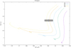 |
Fig. A.1. Hertzsprung-Russell diagram with PMS evolutionary tracks from Siess et al. (2000). The colored lines correspond to different masses (in M⊙). The gray rectangle highlights our values of Teff and L⋆ with their error bars. |
Appendix B: Photospheric absorption lines
Figure B.1 shows the Stokes V and Stokes I profiles of the photospheric absorption lines for both epochs. Table B.1 lists the values of the Blos, the line-of-sight magnetic field integrated over the visible hemisphere, for the photospheric absorption lines.
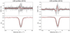 |
Fig. B.1. Stokes V and Stokes I profiles (in gray) and average (in red) of the absorption lines, for the 2010 (left panels) and 2012 (right panels) observations. |
Blos for the photospheric absorption lines.
Appendix C: Emission lines
The emission lines associated with accretion shocks have multiple components (usually a broad and a narrow component). The narrow component is believed to come from the accretion shock, and that is the component we wish to isolate to probe the magnetic field in the shock region. We fit several components of each emission line that we studied and then subtracted all the components except the narrow one, to get a residual profile. Figure C.1 shows two examples, for the HeI line (at 587.6 nm) and for the average of the CaII IRT (at 849.8 nm, 854.2 nm and 866.2 nm).
Table C.1 lists the values of the Blos, the line-of-sight magnetic field integrated over the visible hemisphere, for the HeI line and the CaII IRT.
Table C.2 lists the values of the equivalent width (EW) of the HeI line.
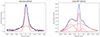 |
Fig. C.1. Fit of the HeI line for the first night of the 2010 ESPaDOnS observations (left panel) and of the average of the CaII IRT for the second night of the 2012 ESPaDOnS observations (right panel). The observed line is in black. The different components are in red and their sum is in blue. |
Blos for the emission lines.
EW of the HeI line.
Appendix D: Bidimensional periodograms
Fig. D.1 shows the bidimensional periodograms of the intensity of the HeI (at 587.6 nm) emission line, the Stokes I and Stokes V LSD profiles of the photospheric absorption lines. Bidimensional periodograms analyze the intensity of the line in several bins over the velocity range. This allows us to see if different parts of the lines have different periods and therefore distinct origins. A dark color on the plots indicates a peak in the periodogram, meaning that a period was found, but a large spot indicates a large uncertainty.We would expect to find the same period in all the bins if the entire line has a single origin. This is seen for instance in the plot of the HeI line in 2010, where the same period is found for the whole redshifted part of the line. However, the width of the peak of the periodogram is very broad, indicating that there is a large uncertainty in this period.
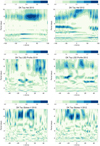 |
Fig. D.1. Bidimensional periodograms of the intensity of the HeI (at 587.6 nm) emission line (top panel), the Stokes I (middle panel) and Stokes V LSD profiles (bottom panel) of the photospheric absorption lines, for the 2010 (left panels) and 2012 epoch (right panels). The power of the periodogram is showed using the color code. A light color represents a zero power intensity, while a dark color represents the maximum power intensity. |
Appendix E: Hα lines
Fig. E.1 shows the Hα line for the fourth and fifth night of the 2010 ESPaDOnS observations, corresponding to phase ∼0.5. For both nights, we see a small redshifted absorption, indicating that the accretion column is in our line-of-sight.
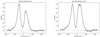 |
Fig. E.1. Hα line for the fourth night (right panel) and the fifth night (left panel) of the 2010 ESPaDOnS observations. The dotted line highlights the continuum. |
All Tables
All Figures
|
Fig. 1. Veiling (gray dots), the best linear fit (blue line) and the standard deviation (light blue shaded region) as a function of wavelength for the fourth night of the 2010 ESPaDOnS observations (top panel) and for the seventh night of the 2012 ESPaDOnS observations (bottom panel). |
| In the text | |
|
Fig. 2. LSD profile (in the heliocentric velocity frame) of Stokes V (top) and Stokes I (bottom) parameters normalized to the continuum for the sixth night of the 2010 ESPaDOnS observations. Note on this night scattered light from the Moon caused the small blue-ward absorption feature. For comparison, we also show the seventh night of the 2010 ESPaDOnS observations (dashed line), which did not suffer from moonlight contamination. |
| In the text | |
|
Fig. 3. Average line-of-sight magnetic field Blos as derived from the photospheric absorption lines and veiling over time, shown folded in phase with the derived 8.2 day period, for the 2010 (left panel) and 2012 (right panel) datasets. Different colors and symbols represent different rotation cycles. |
| In the text | |
|
Fig. 4. Stokes V and Stokes I profiles (in gray) and average (in red) of the HeI emission line (top panels) and the CaII IRT (bottom panels), for the 2010 (left panels) and 2012 (right panels) observations. |
| In the text | |
|
Fig. 5. Average line-of-sight magnetic field Blos over time, shown folded in phase with an 8.2 day period, for the HeI emission line (top panels) and the Ca II IRT (bottom panels), for the 2010 (left panel) and 2012 (right panel) datasets. Different colors and symbols represent different rotation cycles. |
| In the text | |
|
Fig. 6. Equivalent width (in Å) of the HeI emission line over time, shown folded in phase with an 8.2 day period, for the 2010 (left panel) and 2012 (right panel) datasets. Different colors and symbols represent different rotation cycles. |
| In the text | |
|
Fig. 7. Sketch (not to scale) showing DK Tau in the center, surrounded first by its inner disk, then by its outer disk which is considerably misaligned. The rotation axis at 58° is in red, the outer disk axis at 21° is in blue, and the line-of-sight axis is in gray (by C. Delvaux). |
| In the text | |
|
Fig. A.1. Hertzsprung-Russell diagram with PMS evolutionary tracks from Siess et al. (2000). The colored lines correspond to different masses (in M⊙). The gray rectangle highlights our values of Teff and L⋆ with their error bars. |
| In the text | |
|
Fig. B.1. Stokes V and Stokes I profiles (in gray) and average (in red) of the absorption lines, for the 2010 (left panels) and 2012 (right panels) observations. |
| In the text | |
|
Fig. C.1. Fit of the HeI line for the first night of the 2010 ESPaDOnS observations (left panel) and of the average of the CaII IRT for the second night of the 2012 ESPaDOnS observations (right panel). The observed line is in black. The different components are in red and their sum is in blue. |
| In the text | |
|
Fig. D.1. Bidimensional periodograms of the intensity of the HeI (at 587.6 nm) emission line (top panel), the Stokes I (middle panel) and Stokes V LSD profiles (bottom panel) of the photospheric absorption lines, for the 2010 (left panels) and 2012 epoch (right panels). The power of the periodogram is showed using the color code. A light color represents a zero power intensity, while a dark color represents the maximum power intensity. |
| In the text | |
|
Fig. E.1. Hα line for the fourth night (right panel) and the fifth night (left panel) of the 2010 ESPaDOnS observations. The dotted line highlights the continuum. |
| In the text | |
Current usage metrics show cumulative count of Article Views (full-text article views including HTML views, PDF and ePub downloads, according to the available data) and Abstracts Views on Vision4Press platform.
Data correspond to usage on the plateform after 2015. The current usage metrics is available 48-96 hours after online publication and is updated daily on week days.
Initial download of the metrics may take a while.