| Issue |
A&A
Volume 677, September 2023
|
|
|---|---|---|
| Article Number | A158 | |
| Number of page(s) | 26 | |
| Section | Numerical methods and codes | |
| DOI | https://doi.org/10.1051/0004-6361/202346064 | |
| Published online | 21 September 2023 | |
Deep learning denoising by dimension reduction: Application to the ORION-B line cubes
1
IRAM,
300 rue de la Piscine,
38406
Saint Martin d’Hères, France
e-mail: This email address is being protected from spambots. You need JavaScript enabled to view it.
2
Univ. Grenoble Alpes, Inria, CNRS, Grenoble INP, GIPSA-Lab,
Grenoble,
38000, France
3
LERMA, Observatoire de Paris, PSL Research University, CNRS, Sorbonne Universités,
75014
Paris, France
4
Université de Toulon, Aix Marseille Univ., CNRS, IM2NP,
Toulon, France
5
Instituto de Física Fundamental (CSIC).
Calle Serrano 121,
28006,
Madrid, Spain
6
Chalmers University of Technology, Department of Space, Earth and Environment,
412 93
Gothenburg, Sweden
7
Univ. Lille, CNRS, Centrale Lille, UMR 9189 – CRIStAL,
59651
Villeneuve d’Ascq, France
8
LERMA, Observatoire de Paris, PSL Research University, CNRS, Sorbonne Universités,
92190
Meudon, France
9
Laboratoire d’Astrophysique de Bordeaux, Univ. Bordeaux, CNRS, B18N, Allee Geoffroy Saint-Hilaire,
33615
Pessac, France
10
Instituto de Astrofísica, Pontificia Universidad Católica de Chile,
Av. Vicuña Mackenna 4860,
7820436
Macul, Santiago, Chile
11
Institut de Recherche en Astrophysique et Planétologie (IRAP), Université Paul Sabatier,
Toulouse Cedex 4, France
12
GEPI, Observatoire de Paris, PSL University, CNRS,
5 place Jules Janssen,
92190
Meudon, France
13
Laboratoire de Physique de l'Ecole normale supérieure, ENS, Université PSL, CNRS, Sorbonne Université, Université de Paris,
Sorbonne Paris Cité,
75005
Paris, France
14
Jet Propulsion Laboratory, California Institute of Technology,
4800 Oak Grove Drive,
Pasadena, CA
91109, USA
15
National Radio Astronomy Observatory,
520 Edgemont Road,
Charlottesville, VA,
22903, USA
16
Harvard-Smithsonian Center for Astrophysics,
60 Garden Street,
Cambridge, MA
02138, USA
17
School of Physics and Astronomy, Cardiff University,
Queen’s buildings,
Cardiff
CF24 3AA, UK
18
AIM, CEA, CNRS, Université Paris-Saclay, Université Paris Diderot,
Sorbonne Paris Cité,
91191
Gif-sur-Yvette, France
Received:
2
February
2023
Accepted:
18
July
2023
Abstract
Context. The availability of large bandwidth receivers for millimeter radio telescopes allows for the acquisition of position-position-frequency data cubes over a wide field of view and a broad frequency coverage. These cubes contain a lot of information on the physical, chemical, and kinematical properties of the emitting gas. However, their large size coupled with an inhomogenous signal-to-noise ratio (S/N) are major challenges for consistent analysis and interpretation.
Aims. We searched for a denoising method of the low S/N regions of the studied data cubes that would allow the low S/N emission to be recovered without distorting the signals with a high S/N.
Methods. We performed an in-depth data analysis of the 13CO and C17O (1–0) data cubes obtained as part of the ORION-B large program performed at the IRAM 30 m telescope. We analyzed the statistical properties of the noise and the evolution of the correlation of the signal in a given frequency channel with that of the adjacent channels. This has allowed us to propose significant improvements of typical autoassociative neural networks, often used to denoise hyperspectral Earth remote sensing data. Applying this method to the 13CO (1–0) cube, we were able to compare the denoised data with those derived with the multiple Gaussian fitting algorithm ROHSA, considered as the state-of-the-art procedure for data line cubes.
Results. The nature of astronomical spectral data cubes is distinct from that of the hyperspectral data usually studied in the Earth remote sensing literature because the observed intensities become statistically independent beyond a short channel separation. This lack of redundancy in data has led us to adapt the method, notably by taking into account the sparsity of the signal along the spectral axis. The application of the proposed algorithm leads to an increase in the S/N in voxels with a weak signal, while preserving the spectral shape of the data in high S/N voxels.
Conclusions. The proposed algorithm that combines a detailed analysis of the noise statistics with an innovative autoencoder architecture is a promising path to denoise radio-astronomy line data cubes. In the future, exploring whether a better use of the spatial correlations of the noise may further improve the denoising performances seems to be a promising avenue. In addition, dealing with the multiplicative noise associated with the calibration uncertainty at high S/N would also be beneficial for such large data cubes.
Key words: methods: data analysis / methods: statistical / ISM: clouds / radio lines: ISM / techniques: image processing / techniques: imaging spectroscopy
© The Authors 2023
 Open Access article, published by EDP Sciences, under the terms of the Creative Commons Attribution License (https://creativecommons.org/licenses/by/4.0), which permits unrestricted use, distribution, and reproduction in any medium, provided the original work is properly cited.
This article is published in open access under the Subscribe to Open model. This email address is being protected from spambots. You need JavaScript enabled to view it. to support open access publication.
1 Introduction
The current generation of millimeter radio-astronomy receivers is able to produce large spectro-imaging data cubes (about 106 pixels ×105 frequencies or 0.4 TB) at a sensitivity of 0.1 K (per pixel of ~9″ × 9″ × 0.5 km s−1 in about 1000 h of observing time at, for example, the IRAM (Institut de Radioastronomie Millimétrique) 30m telescope (Pety et al. 2017). The next generation of receivers will be between 25 and 50 times faster (Pety et al. 2022). Such projects will thus move from the category of large programs, which are difficult to carry out because they require more than 100 h of telescope time per semester, to typical programs that only require 20–40 h per semester. The main challenges in interpreting these observations are the following: (i) the noise level depends on the frequency, (ii) the emission varies from bright unresolved sources to faint extended ones, and (iii) the intricate gas kinematics of the emitting gas leads to complex emission line profiles (non-Gaussian profiles, high velocity line wings, self-absorptions, etc.), which vary from one pixel to another. Increasing the signal-to-noise ratio (S/N), often simply referred to as denoising, is an important step to lead to new discoveries by enlarging the space of achieved observing performances.
Denoising is an important topic in remote sensing, and many methods and algorithms are found in the literature, for instance principal component analysis (PCA, e.g., Wold et al. 1987), kernel-PCA (e.g., Schölkopf et al. 1997), low rank tensor decomposition (e.g., Harshman et al. 1970), and total variation methods (e.g., Vogel & Oman 1996). These methods try to compress and uncompress the input data in a way that filters the noise but retains the salient features of the signal. Among them, autoencoder neural networks are interesting algorithms because they propose a generic nonlinear PCA, well adapted to hyperspec-tral data in Earth remote sensing (Licciardi & Chanussot 2018).
In this paper, we explore the statistical nature of signal and noise in millimeter radio-astronomy cubes in order to understand the adaptations of typical autoencoders, which are required to efficiently denoise these cubes.
This article is organized as follows. Section 2 presents the general problem of denoising and the particular case of denois-ing by dimension reduction. Section 3 details the acquisition processes that directly affect the properties of the noise. Sections 4 and 5 characterize the signal and noise properties for the studied line data cubes. The intrinsic dimension of the signal is determined in Sect. 6. Section 7 presents the modifications proposed to typical autoencoder neural networks to better handle radio-astronomy line cubes. The obtained denoising performances are then compared with the state-of-the-art Regularized Optimization for Hyper-Spectral Analysis (ROHSA) algorithm in Sect. 8. Section 9 summarizes the conclusions.
2 Denoising by dimension reduction
2.1 Definition of a denoising algorithm
The observed data d are noisy observations of the astronomical signal s
 (1)
(1)
where f is a known function that describes the observing process with its random component considered as noise. Denoising computes an estimate ŝ of the signal based on prior knowledge of the deterministic and random part of the function f. This study will be restricted to the case where the response f of the telescope is linear
 (2)
(2)
where n is one realization of an additive random variable N, and c is one realization of a multiplicative random variable C. The variables N and C are centered on 0 and 1, respectively. In radio-astronomy, N represents the thermal noise, and C the calibration noise associated to the uncertain determination of the calibration parameters (see Sect. 5). It is often assumed that the calibration uncertainty is negligible. In this case, the performance of the denoising estimator can be characterized by the improvement of the S/N.
2.2 Supervised versus self-supervised methods
In machine learning, denoising algorithms belong to two main categories.
Supervised methods. that use a set of known (d, s) couples, called a training set, to train the algorithm to estimate s from the measured values of d. When available, ground truth data are the best choice to build the training set. In astrophysics, numerical simulations based on physical laws and laboratory experiments are used as surrogates. The simplifications required to be able to describe a complicated reality may bias the denoising.
Self-supervised methods. consider that data are both the measurements (features) and ground truth (labels). Additional constraints on the denoising process are required to avoid delivering the data itself as the denoised estimate of the signal. A common assumption is that the signal s is located in a lower dimension space than the observed data d. The idea is that the intrinsic dimension of the signal space is lower than its extrinsic dimension. For instance, we shall assume that the data are composed of three features (d1, d2, d3) with four different samples for each of the feature, as in
![Mathematical equation: $\left[ {{d_1},{d_2},{d_3}} \right] = \left[ {\matrix{ 2 \hfill & 1 \hfill & 1 \hfill \cr 1 \hfill & { - 2} \hfill & 1 \hfill \cr 5 \hfill & 6 \hfill & 4 \hfill \cr 2 \hfill & { - 8} \hfill & 4 \hfill \cr } } \right].$](/articles/aa/full_html/2023/09/aa46064-23/aa46064-23-eq3.png) (3)
(3)
The extrinsic dimension is three, that is the number of features. But its intrinsic dimension is only two. Indeed, the values of the features (i.e., the first, second, and third columns of the above matrix) are deterministically linked to two independent variables u and v through
 (4)
(4)
![Mathematical equation: $\left[ {u,\upsilon } \right] = \left[ {\matrix{ {\,\,\,1} & 1 \cr { - 1} & 2 \cr {\,\,\,\,2} & 3 \cr {\, - 2} & 4 \cr } } \right]. $](/articles/aa/full_html/2023/09/aa46064-23/aa46064-23-eq5.png) (5)
(5)
Any algorithm that is able to deduce the above relations from the measured data would enable one to compress it because only two numbers per sample are required to encode the three features. But it would also enable one to denoise the data. Indeed, in the presence of noise, knowing the relationship that exists between the features, will enable us to consider the measurement of the three features as three independent measurements of the same two underlying variables u, v, and thus to increase the S/N of the estimated signal.
2.3 Generic denoising by dimension reduction
2.3.1 Principle
Denoising by dimension reduction aims at mapping the data with an encoder function ℰ : ℝm → ℝl with l < m, so that ϕ = ℰ(d) contains all the salient features ϕ of the signal of interest s and filters out the noise. The fact that l < m implies that the encoder compresses the data. Another function, named decoder Ɗ : ℝl → ℝm, estimates the signal s from its salient features without loss. The estimated signal should preserve the relevant physical information from the astronomical source, and it should have an increased S/N. The spaces ℝm and ℝl are thus called data and bottleneck (or latent) spaces, respectively. The denois-ing will be all the better when l ≪ m, and the signal is extracted without distortion.
In astrophysics, denoising can be achieved with two different approaches. First, astronomers may just wish to improve the S/N of the measurements to ease the extraction of the physical information in a second step. The structure and unit of the estimated signal stay unchanged. Second, astronomers may directly try to estimate the physical parameters (e.g., the source geometry and kinematics, the volume and column density, the kinetic temperature, the far-UV illumination, the Mach number, the magnetic field, chemical abundances, etc.), which best fit the measured data. In this case, the significant physical and chemical processes are selected, and their corresponding laws allow one to fit the data. The salient features ϕ are the physical parameters of interest. While this study will use the first approach, an interesting challenge of denoising algorithms by dimension reduction is to enable astrophysicists to relate the delivered salient features to the physical quantities of interest. For instance, Gratier et al. (2017) showed that the first component of the PCA of the integrated intensities of a set of lines is related to the gas column density.
2.3.2 In practice
Denoising by dimension reduction is thus based on a structure linking data d, estimated signal ŝ, and salient features ϕ as
 (6)
(6)
In principle, the level of distorsion should be measured as the distance between s and ŝ. However, it is impossible here because astronomical observations of the interstellar medium do not provide ground truth. We thus replace ŝ by s in the reminder of the paper for the sake of simplicity. In this representation, (i1 ,…, im) are the spectral channels of the observed intensities, while (j1,…, jl) are the indices of the salient features. The global denoising function A, often called autoencoder, is defined as
 (7)
(7)
It is just the composition of the ℰ and Ɗ functions. The functions ℰ and Ɗ are not exactly inverse of each other. Indeed, in order to denoise, the function ℰ must filter out the noise. In other words, we expect that the function ℰ will transform a random variable D of a large variance into a random variable Φ of a low variance. There is no such requirement for the function Ɗ. For instance, denoising can sometimes be achieved through the association of PCA, which is a linear inversible transformation, with a low dimensional projection. After the application of the PCA to the data, the components that better explain the correlations of the original data are kept and the other ones are set to zero, before inversing the PCA transformation. In this case, Ɗ is the inverse of the PCA, while β is the PCA itself followed by a nonlinear function that sets the noisiest (least informative from the signal viewpoint) components to zero. In this case, the reduction of dimensionality is obtained by enforcing a low dimensional bottleneck with the direct transform before applying the inverse transform.
To achieve the denoising, it is necessary to estimate the best functions ℰ and Ɗ in terms of quality of reconstruction of the data for a given dimensionality of the bottleneck space.
Sampling the data. Finding functions by numerical means first implies to correctly sample the manifold that links their input and output values. In other words, the algorithm must be trained with many (e.g., K) samples of the data d. This is subject to interpretation. In our case, the data are one position-positionchannel cube d(ix, iy·ic), where ix, iy, and ic are the position of a pixel along the position and channel axes. This data cube can be seen as a set of images  (ix, iy) or a set of spectra
  (ic). The molecular line profiles are broadened by the gas motions along the line of sight. Optically thin lines deliver an approximation of the probability distribution function (PDF) of the velocity component parallel to the line of sight. As the interstellar medium is highly turbulent, the different spectra of one cube can be seen as the PDFs of many realizations of the underlying turbulent velocity field. This is the viewpoint used in this article.
Measuring the distance between s and d over all the samples. Our goal is to find a single pair of functions (ℰ, Ɗ) that correctly autoencodes all the samples of the data (all the spectra in our case). The distance between s and d is quantified with the mean squared error (MSE) between d and s over all the samples
 (8)
(8)
The denoising problem can then be recast as an optimization problem whose goal is to find the function 𝒜 that will minimize the distance between s = 𝒜(d) and d, that is
 (9)
(9)
![Mathematical equation: ${\cal L}\left( {A,d} \right) = {1 \over K}\,\,\sum\limits_{k = 1}^K {\,{{\left[ {A\left( {{d_k}} \right) - {d_k}} \right]}^2}} .$](/articles/aa/full_html/2023/09/aa46064-23/aa46064-23-eq12.png) (10)
(10)
ℒ is often called the loss function.
We now need to define the family of functions from which 𝒜 will be selected. Several ways can be used to reach this goal.
Using generic function approximators. Such as artificial neural networks. This will be our choice in this paper (see Sect. 6).
Using specific classes of function. For instance, Marchal et al. (2019) propose to fit the spectra as a finite set of Gaussian functions whose parameters (amplitude, position, full width at half maximum) can be spatially regularized. This methods is named ROHSA that stands for Regularized Optimization for Hyper-Spectral Analysis. In this case, D is a sum of Gaussians, β is the fitting algorithm, and the loss function is regularized as
 (11)
(11)
 (12)
(12)
where 𝒦 is a 2D convolution kernel that computes the second order differences, and λa, λµ, and λσ are the Lagrangian multipliers associated with convolved images of the amplitudes aɡ, positions µɡ, and standard deviations σɡ of the G Gaussian functions. The value of these multipliers needs to be fixed.
3 Acquisition of radio-astronomy spectral line cubes by a ground-based single-dish telescope
A detailed analysis of the radio-astronomical data is of critical importance to understand the specificities of the considered data and thus propose adequate optimizations for the denoising autoencoder. To do this, we first describe the acquisition of the data in detail to emphasize all the phenomena that will impact the properties of the recorded signal and noise.
3.1 The ORION-B IRAM 30 m Large Program
The ORION-B project (Outstanding Radio-Imaging of OrioN-B, co-PIs: J. Pety and M. Gerin) is a large program of the IRAM 30 meter telescope that aims to improve our understanding of physical and chemical processes of the interstellar medium by mapping about half of the Orion B molecular cloud over ~85% of the 3 mm atmospheric window. The ORION-B field of view covers five square degrees at a typical angular resolution of 27″ (or 50 mpc at a distance of 400 pc), or about 8 × 10⁴ independent lines of sight.
It uses the EMIR heterodyne receivers (Carter et al. 2012) coupled with the Fourier Transform Spectrometers (Klein et al. 2006, 2012) that instantaneously deliver two spectra per polarization of 7.8 GHz-bandwidth sampled every 195 kHz. These two spectra, named lower and upper side-bands, are separated by 7.9 GHz. The local oscillator of the heterodyne receiver can be tuned at 3 mm from 82.0 to 107 GHz. This enables a frequency coverage ranging from 70.7 to 118.3 GHz in a few successive observations. Moreover, the horizontal and vertical polarizations are recorded and averaged. This delivers the total intensity of the source (independent of the polarization state). It also allows us to gain a factor of two on the acquisition time compared to recording a single polarization state and assuming that the signal is unpolarized.
The ORION-B large program delivers a total bandwidth of about 40 GHz at a channel spacing of δ f = 195 kHz, that is about 200 000 channels. The spectral resolving power (defined as f / δ f, where f is the observing frequency) increases from 3.6 × 10⁵ to 6.0 × 10⁵ with increasing frequency in the 3 mm wavelength range. This huge resolving power allows radioastronomers to resolve the profiles from emission lines of chemical tracers of the molecular gas, for instance, the J =1–0 lines of the isotopologues of carbon monoxide: 12CO, 13CO, C18O, and C17O.
3.2 Scanning strategy
The heterodyne receivers currently available at the IRAM 30 meter telescope can only record the emission toward a single direction of the sky at any time. They are thus called single-beam receivers. To make an image with such a detector, we need to scan the sky at a constant angular velocity along lines of constant right ascension or declination. The signal is continuously recorded and dumped at regular time intervals. This observing mode is called on-the-fly observations.
The data consist of a set of spectra that cover the target field of view in a set of parallel lines. The angular distance (Δθ) between the lines is set to satisfy the Nyquist sampling criterion
 (13)
(13)
where λ is the smallest observed wavelength, and D is the single-dish telescope diameter (30m here).
The resulting telescope response is slightly elongated along the scanning direction because it is convolved along this direction with a boxcar filter whose size corresponds to the angular size scanned during the integration time (Mangum et al. 2007). To minimize this effect, it is desirable that the telescope has moved only by a small fraction of its natural response during one integration. We choose to dump the data 5 times over the angular scale corresponding to the telescope natural beamwidth
 (14)
(14)
We use the minimum sampling time that the computer system is able to sustain during the typical duration of an observing session, for instance 8 h. With a dump time of 0.25 s, a scanning speed of 17″/s ensures a sampling of 5 dumps per beam along the scanning direction at the 21.2″ resolution reached at the highest observed frequency for the used tuning, that is 116 GHz. The spatial sampling rates along and across the scanning direction are adapted to the highest frequencies of each individual tunings.
Only one scanning direction per tuning was observed in order to maximize the observed field of view in the allocated telescope time. The usual redundancy between horizontal and vertical scanning coverages could thus not be exploited to improve the denoising algorithm.
Studied molecular lines.
3.3 Calibration
Appendix B describes the methods used to calibrate the data. Under perfect conditions, the calibrated spectrum, Scal, can be written as
 (15)
(15)
where Tsys(f) is the system temperature during the observation, ON( f, θl, θm) is the spectra on-source at the position (θl, θm), and REF(f, θl0, θm0) is a reference spectrum observed at a fixed position (θl0, θm0) of the sky where the source does not emit. This reference spectrum is used 1) to correct for the shape of the frequency bandpass, and 2) to subtract the contribution of the atmosphere to the measured signal. The RMS noise level will be directly proportional to the system temperature that is the calibration factor needed to get the right intensity units. Using the same reference spectrum for several adjacent pixels introduces a slight spatial correlation in the noise properties. Section 5.2 characterizes this in detail.
3.4 Spectral resampling and spatial gridding
We wish to study the variations of the emission of a given line as a function of the position on the sky. We thus need to obtain a position-position-frequency cube centered around the line rest frequency in the source rest frame (see Table 1), which is tagged by the typical velocity of the source in the LSRK frame. However, the gas in a molecular cloud experiences turbulent motions. These hypersonic motions imply a combination of a broadening of the linewidth compared to the natural thermal linewidth and a shift in frequency of the line peak due to the Doppler effect associated with the large scale velocity gradients. Both effects are used to probe the kinematics of the molecular gas where star forms (see, e.g., Orkisz et al. 2017, 2019; Gaudel et al. 2023).
In order to study the kinematics of the gas traced by different molecules, it is easier to compare spectral line cubes that share the same spatial and velocity grid. Appendix A describes the impact of the Doppler effect on radio-astronomy line cubes. The velocity axis is linked to the frequency axis through Eq. (A.1). In particular, the velocity resolution associated for a given line is inversely proportional to the line rest frequency for a spectrum regularly sampled in frequency. Getting the same velocity axis for the different tracers around their rest frequencies requires resampling the spectra in velocity. We choose to resample all the spectra to 0.5 km s−1, which corresponds to the spectrometer velocity channel spacing at the highest observed frequency in our data, that is the frequency of the 12CO (1–0) line. This means that all other spectral line cubes will be oversampled along the spectral axis. As the imperfect Doppler tracking also implies a resampling of the spectral axis, we correct for both effects in a single resampling step. This resampling is done by simple linear split (or integration) of the adjacent channels when the target spectral resolution is narrower (or respectively wider) than the original one. This ensures that the line flux is conserved.
At this point, the data are thus a set of spectra regularly sampled on the same velocity grid. They are also regularly sampled spatially but with small spatial shifts between two rows along the scanned direction because the data acquisition only starts when the telescope scanning velocity is constant, and this event has a relatively uncertain position on the sky for each line. We thus need to “grid” the spectra on a regular spatial grid. This is done through a convolution with a Gaussian kernel of full width at half maximum approximately one-third of the IRAM 30 m telescope beamwidth at the considered rest line frequency. This operation conserves the flux and degrades the telescope point spread function width by ~9%. Here again we choose the same spatial grid for all the lines. We set the pixel size of 9″ in order to comply with the Nyquist criterion for the studied line that has the highest frequency. The other spectral line cubes will be spatially oversampled.
We now end up with one position-position-velocity cube per studied line. Each cube contains 240 velocity channels times 1074 × 758 pixels. The size of the voxels are 9″ × 9″ × 0.5 km s−1. The velocity axis is centered around the rest frequency of the associated line. While the spatial and spectral grid are common to all cubes, the spatial and spectral response inversely scales as the line rest frequency. To ease the computation of line ratios, the cubes are often convolved with a Gaussian kernel to reach the same angular resolution as the telescope response of the line that has the smallest rest frequency. This is the case for the cubes provided in the first public data release of the ORION-B project1, where the provided cubes are smoothed to a common resolution of 31″ .In contrast, no action is in general taken to get a common spectral resolution because a large fraction of the analysis just relies on the intensity integrated on the full line profile.
4 Properties of the signal in two ORION-B spectral line cubes
We here analyze the signal properties of two radio-astronomy line cubes from the ORION-B dataset (namely, the 13CO J =1–0 and C17O J =1–0 cubes2). This analysis will lay out the ground for the innovations proposed in Sect. 7.
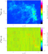 |
Fig. 1 Comparison of mean intensity images between two radio-astronomy lines. |
4.1 Spatial and spectral means
A spectral cube contains two spatial dimensions and a spectral dimension. Figure 1 compares the map of the emission averaged over the spectral axis for the two cubes. The most obvious differences are the intensity dynamics (defined as the ratio of the cube peak intensity to the typical noise level) and the S/Ns. The 13CO (1–0) mean emission has an intensity dynamic of at least a factor 10. But a fraction of the voxels of the 13CO (1–0) cube still lies at S/N lower than 5. The C17O (1–0) mean emission mostly looks like noise. Only an astronomer knowing the shape of the source may guess the existence of some signal on the southeastern part of the image near NGC 2023 and NGC 2024.
Figure 2 compares the spectra averaged over the observed field of view, as well as the minimum and maximum spectra for the two cubes. The line signal is sparse along the spectral axis: The mean spectra of the line cubes show signal only between about −0.5 and 16.0 km s−1, that is a small fraction of the measured channels. These spectra confirm the difference already seen for the intensity dynamics and S/Ns. The sparsity of the line signal along the spectral axis allows us to estimate the noise level. Assuming that the noise follows a centered Gaussian distribution of RMS σ, the difference between the minimum and maximum spectra is 6σ for 99.7% of the samples. This gives a typical noise level of about 0.1 K in our case. The dynamical range of the line cubes are thus on the order of 430 and 20 for the 13CO (1–0) and C17O (1–0) lines, respectively. The spectra in the C17O (1–0) cube must be spatially averaged in order to clearly detect a mean spectrum because the typical S/N of this cube is on the order of 1.
4.2 Histograms of the measured intensities
Figure 3 compares the histograms of the intensities for the two cubes. On each panel, three noise histograms are displayed: The black one uses all the channels, while the green and red ones use the channel with mostly signal or noise, respectively. The left column shows the histograms over the full interval of intensities. These “signal” histograms show that the bright end of the 13CO (1–0) intensities follow an exponential distribution. The right column zooms in over the faint intensity edge of the histogram. These two “noise” histograms are close to a Gaussian distribution. They are centered on zero by construction because of the baseline removal.
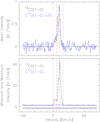 |
Fig. 2 Comparison of intensity spectra between the two radio-astronomy lines. The spectra show the mean (top), minimum and maximum (bottom) intensity as a function of the channel velocity or number. The vertical dashed red lines show the channels whose spatial distribution is plotted on Fig. 4. The vertical dotted lines on the radio-astronomy spectra separate the signal channels from the noise-only ones. |
4.3 Signal redundancy among the channels
Figure 4 compares the spatial distribution of the signal for two channels of the 13CO (1–0) cube. The two chosen channels are displayed as the red vertical lines in Fig. 2. They are centered on the two main velocity components of the Orion В molecular cloud (Pety et al. 2017). These channels display different spatial patterns and are thus quasi-independent. In other words, the knowledge of the first pattern provides no information on the shape of the second pattern.
To better quantify this phenomenon, we compute the Pearson correlation coefficient and the mutual information between each pair of channels. The former highlights linear relationships between two channels while the latter is able to capture both linear and nonlinear relationships. The absence of a linear correlation does not mean either independence or the absence of redundancy to be exploited for information extraction. The computation of the mutual information is thus desirable because, as shown by Licciardi & Chanussot (2018), the relations between the channels of hyperspectral cubes are sometimes strongly nonlinear. It quantifies whether one can predict one quantity knowing the other one, even though the relationship is nonlinear. It is equal to 0 if and only if both variables are statistically independent. More details are given in Appendix F. The mutual information is numerically computed by approximating the joint distribution with nearest neighbors (Kraskov et al. 2004). In order to have homogeneous and comparable results, we express the correlation coefficient in bits of information as the mutual information (Gelfand & Yaglom 1959). If ρ(X, Y) is the Pearson correlation coefficient between X and Y, it can be expressed in bits of information through I = −0.5 log2 [l – ρ(X, Y)2]. This quantity diverges when the relationship between the two variables is deterministic. We thus blank the diagonal coefficients.
The top panel of Fig. 5 shows the linear relation between two channels. The linear correlation of the 13CO (1–0) cube has significant values only in two regions: 1) along the diagonal because the spectral response of the radio-astronomy spectrometer is slightly larger than one channel (see Sect. 5.3), and 2) for the [3.15 km s−1] velocity range, where the signal sits. The bottom panel of Fig. 5 shows the image of mutual information that quantifies any relation. Large values of the mutual information gather into two main groups related to the two velocity components of the Orion В cloud at 6 km s−1 and 11 km s−1. Moreover, there is a faint correlation between the two main velocity ranges. In the signal region, the coefficient values fall by a factor of ~ 10 at a typical distance of 3 or 4 channels. We call this distance mutual information scale in Sect. 6.5. In other words, the mutual information scale is small for the 13CO (1–0) cube.
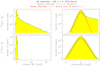 |
Fig. 3 Comparison of the histograms of the intensity of the two radio-astronomy lines. The left column shows the full intensity dynamical range, while the right column zoom on faint intensity. The black histogram is computed over all the data channels. The red and green histograms are computed over the channel ranges that contains either mostly noise or high signal-to-noise ratio intensity, respectively. |
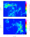 |
Fig. 4 Velocity channels at 6 and 10 km s−1 of 13CO (1–0). The corresponding channels are displayed as vertical dashed red lines in Fig. 2. |
5 Noise properties
We next characterize the noise properties inside the acquired radio-astronomical cubes. In particular we compute the noise spatial and spectral power density3.
5.1 Spatial and spectral levels
To estimate the noise levels, we assume that the spatial and spectral variations of the noise are independent of each other, as proposed by Leroy et al. (2021). The noise RMS can then be factored as
 (16)
(16)
where σspe(ix, iy) and σspa(ic) represent the spatial and spectral variation of the noise RMS computed along the spectral and spatial axes, respectively. We start by computing the noise RMS of the channels for each pixel on channels that are devoid of signal. We then divide the signal cube by the spatial variations of the spectral RMS, σspe(ix, iy), and we compute the RMS per channel after masking regions where signal is detected (see Sect. 7.3). Moreover, we compute the standard deviation of the RMS as  where s is the number of samples used.
The top panel of Fig. 6 shows the map of the noise spectral RMS, normalized by its median value, for the C17O (1–0) cube. We do not show the result for the 13CO (1–0) cube because it is similar to the result for the C17O (1–0) cube. The noise map has an obvious inhomogeneous spatial distribution with mostly vertical stripes organized in squares. This reflects the acquisition scheme, where a single pixel detector is scanned along vertical lines of size of ~1000″ inside squares. The noise pattern evolves from left to right because the scanning strategy was optimized during the acquisition of the ORION-B large program data. For instance, in the middle of the acquisition we tried to organize the approximately 1000″-long scans into long vertical lines instead of squares. However, this increased the striping in the signal images. We thus decided to come back to an acquisition in consecutive squares to ensure a better continuity of the signal.
The noise comes mostly from the atmosphere contribution to the measured power in radio-astronomy (see Appendix C.1). This implies that the noise level follows to first order the quality of the weather. A dry atmosphere during winter observations improve the noise level by a typical factor of approximately 1.5 over summer observations for the two studied lines. This is the origin of the large variations of the noise level from one square to another. The amount of atmosphere that emits depends on the source elevation. It is minimum at zenith and maximum when the source rises and sets. Thus, the noise level also follows the elevation of the telescope at constant weather, and this is the main origin of the noise level regular variations inside each square.
The bottom panel of Fig. 6 shows the variations of the spatial RMS of the noise with the velocity. The line cubes show spectral variations of the noise between −2 and +4% with two characteristic patterns. First, there is an oscillating pattern that directly comes from the resampling of the spectra along the spectral axis. Superimposed, there is also an increase of the noise level of about 2% following more or less a boxcar function between −10 and +30 km s−1. This is related to the baseline removal step during the reduction. This step is required to remove remaining atmospheric residual signal after the atmosphere calibration. It is done by fitting a Chebyshev polynomial of low order outside the velocity window where the signal appears with some margin to avoid biasing the baseline by signal at low S/N in the line wings. The baseline substracted inside the signal window is then interpolated using the fitted Chebyshev coefficients. We here used a polynomial order of degree 1 outside the [−10, +30 km s−1] signal window.
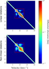 |
Fig. 5 Amount of information shared between channels for the 13CO(1–0) data cube. The top row shows information related only to linear relationship, while the bottom row shows information related to any type of relation (i.e., the mutual information). |
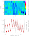 |
Fig. 6 Noise spatial (top) and spectral (bottom) variations for the C17O (1–0) line cube. The spatial maps were normalized by the median noise value. The red region in the bottom panels shows the 3σ uncertainty interval of the computation. |
5.2 Noise spatial power density
We first compute the spatial 2D Fourier transform of the C17O (1–0) cube for 90 channels devoid of signal, from −50 to −5 km s−1. We then compute the square of the modulus of the Fourier transform, and we finally average the 90 resulting images. This gives an estimation of the noise spatial power density.
We use the radio-astronomy convention to define the conjugate coordinates of the angular coordinates (θl, θm) relative to the projection center of the image as (u, v) with
 (17)
(17)
where λ is the wavelength of the observed line. In our case, λ = 2.67 mm. The conjugate planes are called image and uv planes, respectively. The (θl, θm) and (u, v) coordinates are expressed in radian and meter, respectively.
The first column of Fig. 7 shows the obtained noise spatial power density. For a perfect measurement, we expect to recover an image proportional to |ℱ [B]|2, that is the square of the modulus of the Fourier transform of the point spread function of the telescope B. While |ℱ [B]|2 should show a radial symmetry to first order, we obtain a spatial power density that is dominated by a structure elongated along the u axis. This structure comes from correlations in the observed noise between all the spectra belonging to the same subscan (scanned vertically in this case).
Appendix C shows that the noise spatial power density is to first order equal to 𝒫 (u, v) ≃ 𝒫on(u, v) + 𝒫ref(u, v), with
![Mathematical equation: ${P_{{\rm{on}}}}\left( {u,\upsilon } \right) = {A_{{\rm{pix}}}}\,{\left( {{{{\sigma _{{\rm{on}}}}} \over \sigma }} \right)^2}\,\,{\left| {{\cal F}\left[ B \right]} \right|^2}\left( {u,\upsilon } \right),$](/articles/aa/full_html/2023/09/aa46064-23/aa46064-23-eq21.png) (18)
(18)
and
![Mathematical equation: ${P_{\,\,\,{\rm{ref}}}}\left( {u,\upsilon } \right) = {A_{{\rm{rect}}}}\,{\left( {{{{\sigma _{{\rm{ref}}}}} \over \sigma }} \right)^2}\,{\left[ {{\rm{sinC}}\,\left( {{{{\rm{\Delta }}{\theta _l}u} \over \lambda }} \right)\,{\rm{sinC}}\,\left( {{{{\rm{\Delta }}{\theta _m}\upsilon } \over \lambda }} \right)} \right]^2}.$](/articles/aa/full_html/2023/09/aa46064-23/aa46064-23-eq22.png) (19)
(19)
In these equations, Apix and Arect = ΔθlΔθm are the respective areas of the image pixel and of any rectangle that shares the same reference measurement. Moreover,  , and σon and σref are the typical standard deviation of the noise on source and on reference, respectively.
The second and third columns of Fig. 7 show the resulting model, and the ratio of the measured and modeled noise spatial power density in logarithmic scale. In the studied case, the modeling holds for most of the uv plane.
5.3 Noise spectral power density
Figure 8 shows the noise spectral power density and the noise autocorrelation. To get them, we first compute the 1D Fourier transform along the frequency axis for the same subcube devoid of signal. We then compute the square of the modulus of the Fourier transform, and we average results over the pixels. The autocorrelation function of the noise is estimated by calculating the inverse Fourier transform of the spectral power density.
The autocorrelation shows that the correlation between two channels x[f] and x[f + δf] becomes zero when |δf | > 2 × 183.80 kHz. This fact leads us to model the noise spectral autocorrelation with the autocorrelation of a symmetric finite impulse response filter of the form h = [a b a], with the constraint 2a2 + b2 = 1 in order to preserve the signal power. The curve on Fig. 8 shows five nonzero values because it corresponds to the autocorrelation of the filter. We estimate h = [0.18 0.97 0.18] for the 13CO (1–0) and C17O (1–0) spectral cubes. The good fit of the noise autocorrelation with the autocorrelation of this filter indicates that the noises of pair of channels separated by more than two channels are uncorrelated. The estimated filter can be used to simulate noise with a similar spectral power density.
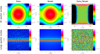 |
Fig. 7 Comparison between the measured (left) and modeled (middle) noise spatial power density, and their ratios (right) in logarithmic scale. The top row shows the spatial power densities for all scales, while the bottom row zooms in on the large spatial scales. |
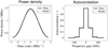 |
Fig. 8 Comparison between the measured (plain line) and modeled (dashed line) spectral power density (left) and autocorrelation function (right). |
5.4 Noise PDFs at low and large S/N
The measured intensity at pixel i j and velocity channel c is given by
![Mathematical equation: ${I_{ijc}} = \left( {1 + {_{ij}}} \right)\,\left[ {{S_{ijc}} + {N_{ijc}}} \right],$](/articles/aa/full_html/2023/09/aa46064-23/aa46064-23-eq24.png) (20)
(20)
where Sijc is the signal from the source, Nijc the additive noise coming mostly from the atmosphere and the receiver, and ϵij the relative uncertainty on the calibration gain. We assume that ϵij is mostly constant over the narrow-band spectra used here. The values of Nijc and ϵij are drawn from two centered normal distributions of standard deviation σijc and Σ, respectively. Depending on the observed atmospheric window (3 or 1 mm), the values of Σ range from 0.05 to 0.1, so ϵij ≪ 1 (for details, see the Appendix D). Thus, there are two main different limiting regimes that depend on the S/N

At low S/Ns, we can neglect the uncertainty of the calibration, and the additive noise dominates the uncertainty budget. In contrast, at a high S/N, we can neglect the additive noise, and the uncertainty budget is dominated by the multiplicative noise with  .
.
6 The autoencoder neural network as a generic method of dimension reduction
In this section, we introduce a deep learning method called autoencoder neural network. We present its default architecture and operation. We then use it to compute the amount of redundancy available in the input dataset. In the next section, we tailor it for molecular line cubes based on the data analysis performed in Sect. 3.
6.1 Neural networks
Artificial neural networks are a class of statistical machine learning methods that were originally designed to simulate the behavior of the brain. Today, they are widely used in data science because they allow any nonlinear functions in high dimensional spaces to be modeled easily. More precisely, we use architectures derived from the multilayer perceptron (Shalev-Shwartz & Ben-David 2014). Multilayer perceptrons are composed of a succession of matrix products and nonlinear functions called activation functions. They are interesting because they are universal approximators of any continuous function when they have at least one hidden layer and this layer contains enough neurons (Hornik et al. 1989). Appendix E gives more details.
The modeling of a nonlinear function by a neural network can be considered as a global optimization problem that is solved through stochastic gradient descent. The user specifies a loss function that will constrain the neural network to select one family of functions adapted to the considered problem. The only constraint on the loss function is that it must be derivable with respect to each parameter of the network, in order to be able to perform their optimization by the stochastic gradient descent algorithm (Duda & Hart 1973).
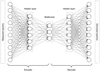 |
Fig. 9 Example of an autoencoder neural network. Each column represents a neuron layer. Each arrow represents a connection between the neuron layers. The first and last layers are composed from the measured and denoised intensities of a spectrum at the different channels, respectively. The bottleneck contains the minimum number of neurons needed to compress the data without loss of signal information. In this example, the signal intrinsic dimension (size of the bottleneck) is three while the data extrinsic one (size of the input and output spectra) is 10. |
6.2 Autoencoder neural network
Figure 9 shows the architecture of an autoencoder neural network. As the autoencoder described in Sect. 2.3, it is composed of two cascaded parts, the encoder and the decoder functions that are implemented as two neural networks. The encoder aims at computing a simplified representation of the data. The decoder aims at reconstructing the input data as faithfully as possible from the simplified representation. In our cases, we choose symmetrical architectures for the encoder and decoder parts. Nevertheless, it does not mean that the functions ℰ and Ɗ are inverse from each other, as explained in Sect. 2.3.
The reduction of dimension space enforced by the autoencoder can be interpreted as an approximation of a nonlinear PCA (Licciardi & Chanussot 2015). In the case of noisy data containing signal with a low dimension representation, this compression should retain the signal features and filter the noise. As an autoencoder neural network is designed to identify a low dimension representation of the signal, it allows one to perform a generic denoising operation. In particular, it generalizes the denoising operation that can be performed with a PCA in the case where the signal features are nonlinearly correlated.
6.3 Estimating the intrinsic dimension of a dataset
When denoising by reduction dimension, the amount of denoising is related to the redundancy in the input data, which allows one to reduce the dimension without loosing relevant information. If the dimension of the input data is called the extrinsic dimension and the dimension of the bottleneck the intrinsic dimension, we thus wish to measure the intrinsic dimension of the data. The extrinsic dimension is necessarily greater than or equal to the intrinsic dimension.
An autoencoder neural network is interesting here because it is a practical algorithm that encompasses the whole category of methods that assumes a reduction of dimension to denoise the data (see Sect. 1). We use the autoencoder to analyze the intrinsic dimension of the signal with respect to the extrinsic dimension of the data, and thus emphasize the amount of redundancy that could be used to increase the S/N.
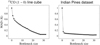 |
Fig. 10 Distance (mean absolute deviation) between input and reconstructed data as a function of the bottleneck size for the 13CO (1–0) data (left) and the Indian Pines data (right). |
6.4 Implementation
We define a set of autoencoders whose bottleneck size varies between one and the extrinsic dimension of the data (m). The loss function is then minimized for each of these autoencoders. Figure 10 shows the mean absolute deviation between the input data and the denoised data as a function of the bottleneck size (l). The intrinsic dimension is the smallest dimension of the bottleneck that allows us to reconstruct the signal without significant loss of relevant information. Two regimes are expected for this curve: A quick decrease of the mean absolute deviation as long as increasing the bottleneck size adds useful information to reconstruct the signal, followed by a constant value of the mean absolute deviation when further increasing the bottleneck size starts to reconstruct the noise. The threshold between these two regimes is interpreted as the intrinsic dimension of the data. This method is directly inspired by the “elbow method” used when denoising with a PCA (Ferré 1995).
The choice of the loss function is key to ensure a proper estimation of the intrinsic dimension. A desirable property is to select encoders that will maintain independent input variables as independent bottleneck neurons instead of encoding them as linear combinations. Using the mean absolute deviation instead of the more usual mean squared error allows one to avoid mixing independant inputs. Indeed, we shall assume that the data are composed of two uncorrelated non-Gaussian (e.g., Laplacian) variables of mean 0 and variance 1. The encoding of this pair of variables with a single component (i.e., an autoencoder with a single bottleneck neuron) consists in searching for the direction that maximizes the norm of the projection in one direction. As illustrated in Fig. 11, the L2 norm is invariant to rotation, implying that the maximization of the projection is not sensitive to rotation, so the encoder will mix the two components. In contrast, the values of the L1 norm varies under rotation, so the autoencoder will thus avoids mixing the independent pair of variables. In other words, if we try to encode the two independent variables with a bottleneck made of a single neuron, the MSE loss function will constrain the autoencoder to pay attention to the largest values of the two random variables and to combine them linearly in order to minimize its value. In contrast, the mean absolute deviation will enforce a solution where only one of the two independent variables is encoded in the bottleneck, the other one being ignored.
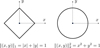 |
Fig. 11 Illustration of the non-invariance to rotation of the L1 norm as opposed to the L2 norm. |
6.5 Comparison of the intrinsic dimension between the ORION-B cubes and a typical hyperspectral cube
Figure 10 compares the evolution of the mean absolute deviation as a function of the dimension of the bottleneck for two datasets: The ORION-B 13CO (1–0) line cube on the left panel, and a Earth remote sensing hyperspectral cube, named Indian Pines4, that is used to benchmark denoising algorithms on the right panel. This comparison is useful because Licciardi & Chanussot (2018) showed that dimension reduction with a neural autoencoder is particularly efficient to denoise the latter dataset.
The intrinsic dimension of Indian Pines can be estimated at around 4. In constrast, the curve for 13CO (1–0) only has a clear elbow at about 27. This implies that the intrinsic dimension of the signal is close to its extrinsic dimension. This confirms our previous finding that the measured mutual information scale is small for the ORION-B line data (see Sect. 4.3).
Two main properties explain the different behaviors of the 13CO (1–0) and Indian Pine cubes. The astronomy line cube contains many signal-less channels that are irrelevant for scientific purpose but can be used to characterize the noise properties. Moreover, the achieved spectral resolution still limits the amount of redundancy inside the sampled line profile. In contrast, almost all the channels of Indian Pine cube are scientifically relevant and (anti-)correlated. In this respect, denoising by dimension reduction would be easier for astronomy hyperspectral cubes observed with direct detection imaging spectrometers used to study the spectral energy distribution of the sources, including the continuum and and low to medium resolution spectral line emission, such as the SPIRE and PACS spectrometers on-board Herschel (Pilbratt et al. 2010) or the MIRI and NIR-Spec instruments on-board JWST (Rigby et al. 2023), because such instruments provide hyperspectral cubes with scientifically relevant information for each spectral channel.
7 A locally connected autoencoder with prior information to denoise line data
As discussed in the previous section, the reduction dimension of the ORION-B line cubes is more difficult than in the case of Earth remote sensing cubes. It is thus all the more important to optimize the structure of the used autoencoder neural network with sound assumptions to help it converge on the correct solution. In this section, we propose an innovative autoencoder structure adapted to the properties of the line cubes. We first describe the geometry of the autoencoder that takes into account the fact that the mutual information scale is small compared to the extrinsic dimension of the data. We then propose a loss function that ensures that channels without signal are set to zero instead of some arbitrary (small) value.
7.1 Locally connected autoencoder
A typical autoencoder is composed of fully connected layers, which means that all the input neurons of the layer are connected to each output neuron (see Fig. 9). This ensures that all potential correlations between the input data are explored. In line cubes, only channels at nearby frequencies are correlated. This means that an autoencoder would try to learn the numerous combinations of uncorrelated channels. Figure 12 shows an architecture where a set of multilayer perceptrons connects adjacent input neurons to adjacent bottleneck and output neurons. In our case, this means that only adjacent channels will be encoded together. This change introduces a major difference compared to a typical autoencoder. The latter would deliver the same result (within numerical approximations) whatever the ordering of the input neurons. In contrast, our tailored autoencoder assumes that adjacent channels are linked together. This means that we introduce the notion of proximity in frequency of the channels inside the autoencoder architecture.
As a comparison, a convolutional layer5 (O’Shea & Nash 2015) would in addition take into account the order of the channels. However, the applied convolution filter would be identical for all observed spectra. In other words, a convolutional layer assumes spectral translation invariance with respect to the observed spectra while the proposed architecture does not. In particular, the fact that the S/N and the amount of signal information can vary significantly with the frequency would be ignored with a convolutional layer.
For simplicity, we choose a symmetric autoencoder which has a total of four hyperparameters that must be chosen: 1) l, the size of the bottleneck layer; 2) p, the size of the sliding window that connects nearby channels; 3) q, the size of each perceptron layer; and 4) h, the number of hidden layers of each perceptron. We have the following relations: l < m and p < q < m, where m is the number of input and output channels in the spectrum. The hyperparameters of the tailored autoencoder may depend on the studied line. For instance, it is likely that the model for a line such as 13CO (1–0) is more complex than for the C170 (1–0) line, implying larger values for l and h. The data analysis performed in Sect. 4.3 imposes some constraints. If r is the mutual information scale in channel units, the optimal window size is p = 2r + 1. Moreover,  is a (potentially optimistic) lower bound for the size of the bottleneck because it represents the number of groups of channels that are decorrelated from each other.
In practice, the simplest implementation of our tailored autoencoder is to perform a matrix product for each window. However, the autoencoder will then perform a large number of consecutive matrix products leading to large overheads. We instead choose to encode the set of locally connected perceptrons as a unique fully connected perceptron, where the superfluous weights are set to 0 during the initialization and the associated gradients are multiplied by 0 during the training. This requires a single (tailored) matrix multiplication per layer. The number of free (i.e., nonzero) parameters in this optimized autoencoder can be computed directly from the Python implementation that is available on the project GitHub repository. In our application, the number of free parameters is only 6% of the total number of matrix elements. This eases the training of the optimized autoencoder.
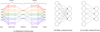 |
Fig. 12 Optimized autoencoder architecture (a) where fully connected layers (b) are replaced by locally connected layers (c). The number of entries is 5 and the bottleneck is size 3. The hidden layers of the network can be described by describing the small encoders, here they are of dimension [3, 2] with input and output windows of the same size 3. |
7.2 Adding prior information to the optimization problem
As described in Sect. 2.3.2, denoising by dimension reduction is an optimization problem that tries to find the autoencoding function 𝒜 that will minimize the distance between the data and its autoencoding, averaged over all the data samples: see Eqs. (9) and (10). The presence of noise implies three adaptations of the autoencoder about the definition of its training loss function. The first one will take into account the important variation of the S/N (from <1 to a few 100) in radio-astronomy data. The second one will address the potential unbalance between the number of voxels that only contain noise and the number of voxels that actually contain relevant signal. The third one will ensure that the autoencoder attributes a zero-valued intensity (instead of any other randomly chosen systematic value) for voxels that only contain noise.
To handle varying S/N values. The distance is usually weighted by the standard deviation of the noise. In our case, the baseline part of the spectrum enables us to easily estimate the noise standard deviation σk for the spectrum dk at pixel k = ix + nx (iy – 1). We thus will modify the loss function as
 (21)
(21)
This normalization avoids the variation of the data “energy” just caused by noise, which would overweight the noisiest pixels. We recognize here the reduced χ-squared merit function that is regularly used in astronomy. In contrast, the machine learning community mostly uses the MSE.
To address the problem of sparsity of the signal inside the cube. We balance the loss function by giving prior information about the channels that have a large probability to be just noise. To do this, we first segment the position-position-frequency cube into signal and noise samples (see Sect. 7.3). We then modify the loss function as
 (22)
(22)
where w jk = 1 for a channel j of spectrum k dominated by signal, and w jk = 0, elsewhere. The normalization factors ensure that noise-only (S /N < 1) samples do not dominate the loss function. This solves the potential unbalance between signal and noise samples inside each spectrum. While the architecture of the optimized autoencoder does not use the spatial information, the segmentation used in the proposed loss function introduces some spatial information as it is a method that works in the position-position-frequency space.
To ensure that noise-only samples deliver 0. Instead of a small random value, we use the Lq norm6, with q ∈]0, 2], for samples that are mostly noise. This enforces the training to choose either 0 or the autoencoded (denoised) value of the data, 𝒜(djk). The denoised value of the data will be selected when the data sample has a statistical signature too far from random Gaussian noise. The hyperparameter q allows one to finely control the asymptotic behavior of the penalty of voxels containing only noise: The closer q is to 0, the larger the penalty applied to an autoencoded value close to zero. In this study, we chose q = 1.
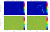 |
Fig. 13 Maps of the maximum (top) and minimum (bottom) S/N per spectrum before (left) and after (right) convolution of the C17O (1–0) line cube by the telescope point spread function. |
7.3 Detecting significant signal
The C17O (1–0) is characterized by a low S/N. The best way to detect signal in such a condition is to correlate the noisy measurement with the expected shape of the signal and to threshold the output because the probability that random noise reproduces the expected shape is negligible. This technique, named matched filtering, is all the more effective when the shape of the signal is accurately known. For example, if one aims at detecting a point source, we just need to know the point spread function of the instrument. Correlating the noisy measurement with the point spread function thus not only delivers an optimal way to detect point sources, but it also improves the detection of spatially resolved sources. Indeed, adjacent pixels can be thought as measurements of the same source where the noise is uncorre-lated from one pixel to another. As the pixel size is chosen to at least Nyquist-sample the point spread function, any source will be spread over at least four contiguous pixels, and the S/N after correlating with the point spread function will be much higher than the S/N per pixel of the original image. As this makes no assumption on the shape of the source, this is a simple way to optimize the detection of any kind of a resolved source. In summary, while matched filtering is the optimal way to detect point sources, it also improves the detection of resolved sources because it smoothes the data to an angular resolution larger by  and thus naturally increases the S/N per pixel.
Figure 13 shows the map of the maximum and minimum S/N per spectrum before and after correlation of the C17O (1–0) line cube by the telescope point spread function. In both cases, the S/N is defined as
 (23)
(23)
where d(ix, iy, ic) and σ(ix, iy, ic) are the position–position–velocity cubes of intensities and noise RMS, respectively. The computation of the noise RMS is described in Sect. 5.1. When correlating the cube by the instrument response, the maximum of the S/N improves by a factor on the order of 2 from 9.7 to 16.8, and the percentage of pixels whose maximum S/N value is above 5 increases from 0.13 to 0.75%. In contrast, the minimum S/N value is relatively stable (−6.7 vs. −6.1) as expected when the noise is (mostly) uncorrelated between adjacent pixels.
The S/N cube can then be thresholded to yield a 3D mask of detected pixels. On one hand, we wish to reduce the number of false positives. This requires to use a relatively high threshold value. Indeed, for a Gaussian additive noise, even using a S/N threshold value of 3 yields about 0.3% of false positives, that is approximately 105 voxels even when assuming that the signal can be present only between −5 and 20 km s−1. On the other hand, we wish to reduce the number of false negatives. In millimeter radio-astronomy, a large fraction of the source flux frequently has S/N values lower than 3. Using a too high S/N threshold value thus implies a large quantity of false negative pixels.
The first way to improve the tradeoff between the requirements to minimize the number of false positives and negatives uses again the fact that the noise distribution is (mostly) uncorrelated between contiguous pixels. It is indeed possible to segment the cube in regions contiguous in the position-position-velocity space and for which all pixels have a S/N value above a given threshold. In practice, we define segments of voxels contiguous in the position–position–velociy space, which satisfy the S/N criterion. When a voxel is added to the current segment, we check whether the segment should be merged with a segment already defined in the previous row of the current image or the previous image of the cube. The pixels that do not satisfy the criterion are put in a specific segment regardless of their position in the cube. Segmenting in contiguous regions above a given threshold was proposed by Pety & Falgarone (2003) along the spectral axis and Rosolowsky & Leroy (2006) in 3D. When adjacent samples have uncorrelated noise levels, the probability of a false negative decreases when the total S/N of the region (defined as the sum of the S/N over all the pixels of the region) increases. Hence sorting the segmented regions by decreasing total S/N and selecting the first few ones minimizes the chance 1) to overlook large regions at relatively low values of the mean S/N, and 2) to yield too many false positive regions.
Figure 14 shows the evolution of three properties of the 3D segments obtained for the C17O (1–0) line, and sorted by decreasing value of the S/N summed over their voxels (hereafter named segment total S/N). The three properties are the number of voxels inside each segment, the segment total and mean S/N. These properties are shown for two different S/N thresholds (1 and 2) used during the cube segmentation process. Figure 15 shows maps of the peak intensity  I(ic), the line integrated intensity
  I(ic)dv, and the centroid velocity
  . We compute them by including the voxels that belong to the first 200 segments. In all generality, the number of segments included is a compromise between including only the segments with the highest total S/N and enough segments with a mean S/N larger than 3. Two hundred segments is a good compromise when the S/N threshold is 2. We here use the same number of segments when the S/N threshold is 1 in order to make a comparison without changing too many parameters at a time.
For the C17O (1–0) line, the number of voxels per segment varies from more than 10 millions to about 1, in comparison with the 195 millions of voxels present in the cube. The total S/N follows a similar trend because the mean S/N per voxel is low. In contrast, the mean S/N and images have a different behavior depending on the S/N threshold.
For a threshold of 1. The segment mean S/N is always smaller than 3. It is constant at about 1.5 before oscillating. Voxels have been selected over almost all the field of view and it is difficult to see any structured signal in the three associated maps.
For a threshold of 2. The segment mean S/N starts to decrease or oscillates above 3 before converging to about 2.5 with an increasing dispersion. The signal is now pretty well defined in the three associated maps, even though some vertical striping is sometimes still visible.
These properties can be understood by the fact that for uncorrelated Gaussian noise, the probability to have the intensity of one of the 6th closest neighbors to any voxels above 1, 2 or 3σ is 0.90 = (1 − 0.6836), 0.25, and 0.02 respectively. This implies that any voxel has a large chance to be part of the first segment for an S/N threshold of 1, a minor chance for a threshold of 2, and a negligible chance for a threshold of 3.
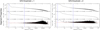 |
Fig. 14 Properties of the segments obtained on the cube of S/N for the C17O (1–0) line. This cube was segmented into contiguous position-position-velocity regions above a minimum S/N value. The segments are ordered by decreasing value of the S/N summed over the segment (total S/N). The shown properties are, from top to bottom, the total number of pixels inside the segment, the total S/N, and the mean S/N of the segment. These properties are shown for two different S/N thresholds: 1 and 2. The blue plain vertical lines show the segments that are selected to compute the moment maps in Fig. 15. The red dashed horizontal lines show the typical mean S/N reached for the segment # 200. |
8 Denoising performances
We here compare the denoising performances between our tailored autoencoder and the ROHSA algorithm7 that we shortly summarized in Sect. 2.3.2. We do this comparison on the 13CO (1–0) cube that displays a large S/N range. Our autoencoder neural network and ROHSA share several properties. They propose a representation of the data that can be interpreted as denoising by dimension reduction. They work mainly on individual spectra with a regularization term that introduces some spatial information about the data. They nevertheless differ in the family of functions assumed to encode the data. ROHSA assumes that the signal is composed of a limited number of Gaussian functions whose amplitude, position, and standard deviation are spatially regularized. Our autoencoder assumes that the data can be approximately classified as noise and signal pixels, and that the scale of mutual information between channels is small compared to the number of channels in the spectra.
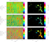 |
Fig. 15 Maps of the moments of the spectrum for two different values (1 at left, and 2 at right) of the S/N threshold used to compute the position– position–velocity mask of significant emission. From top to bottom, the peak intensity (maximum of the spectrum), line integrated intensity (moment 0 of the spectrum), and centroid velocity (moment 1 of the spectrum) are shown. |
8.1 Detailed setups of the autoencoder and ROHSA
We use the Python framework PyTorch to implement our numerical neural network experiments8. The segmentation of the line cubes is implemented in a new IRAM software named CUBE and distributed inside GILDAS9. The associated Python and CUBE scripts are available in a GitHub repository10.
We use the approximately 800 000 spectra of 240 channels as input to the autoencoder. We tagged as mostly signal the voxels that belong to the first 200 segments obtained with a S/N threshold of 2, and the reminders as mostly noise. The hyperparameters of the autoencoder were optimized as follows. The width of the sliding window is set at 7 channels according to the mutual information scale (see Sect. 4.3). Most of the other hyperparameters were set with a typical cross validation procedure (Refaeilzadeh et al. 2009). In short, we first defined a set of possible values to explore. For each set of hyperparameters, we then optimized the network on a training dataset and we compute its performance on a different validation dataset. In order to reduce the variability of the results depending on the choice of the training and validation sets, this procedure is performed several times, varying the test and validation sets so that each sample has been selected once in the validation set during the procedure. This gives for the local encoder: A bottleneck size of 75% the number of input channels (here 180), and 3 hidden layers of size [35, 14, 7] per perceptron. During this cross validation procedure, the hyperparameters that are assumed noncritical are fixed to usual values: The Adam stochastic optimizer (Kingma & Ba 2014) was used with a batch size of 100, 50 epochs, and a learning rate that decreases exponentially from 10−3 to 10−6.
Instead of trying to optimize the hyperparameters of ROHSA for denoising, we used the ones derived by Gaudel et al. (2023) when trying to decompose the spectra into a set of coherent velocity layers in order to study the velocity field around the filaments of gas where stars will form. The number of Gaussians was set to 5 for the 13CO (1–0) cube, and the Lagrangian multipliers used to regularize the maps of Gaussian amplitude, position, and standard deviation were λa = λµ = λσ = 100.
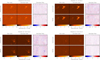 |
Fig. 16 Comparison of the denoising performances of the taylored autoencoder and ROHSA for four different velocity channels belonging to the line wings. For each channel, the raw (left) and denoised (middle) images are shown with the same intensity scale and the residual (right) image is displayed with an optimized intensity scale. The top and bottom rows show the results for the autoencoder and ROHSA algorithms, respectively. |
8.2 Results
Figure 16 compares the raw images with the denoised ones obtained with the autoencoder and ROHSA for four different velocity channels that were chosen in the line wings because denoising of the additive component is expected to act mostly at low to intermediate S/N. The two algorithms produce similar results to first order. They both set noise-only voxels to a value close to zero. The shape of significant signal is kept, and the residuals mostly look like noise. A closer look suggests that ROHSA delivers signals that are more spatially coherent than the autoencoder at low S/N but this stays within the noise level. At intermediate S/N, ROHSA deforms the signal more than the autoencoder as can be seen in the residuals of the channels at 13.5 km s−1.
A more quantitative comparison can be seen in Fig. 17 that shows the spatial variations of the spectral RMS of the residual cubes and their ratio with the spectral RMS of the raw data. The spatial variations of the spectral RMS show that both algorithms recover the rectangular pattern coming from the ON-REF acquisition method. However, a significant part of the signal appears in the ROHSA residuals, while only a few point sources appear in the autoencoder residuals. The signal that remains in the autoencoder residuals is coming from defaults in the signal tagging procedure. The better preservation of the signal by the autoencoder goes hand in hand with a slight under-denoising. Indeed, the map of the spectral RMS of the residuals normalized by the spectral RMS of the noise is on average lower than 1 in regions that have been tagged as mostly signal. In other words, the denoised output is closer to the raw input than it should be in case of perfect denois-ing. In contrast, the residuals of ROHSA better recover the noise level at low S/N at the price of more distortion of the signal at high S/N.
Figure 18 compares the joint histogram of the denoised vs. the raw intensities. A perfect denoising of the noise additive component would deliver a joint histogram along the diagonal at large S/N and an histogram whose dispersion is very asymmetric around zero: The distribution should have the same dispersion as the noise along the raw intensity axis and a narrow dispersion along the denoised intensity axis. The autoencoder succeeds in mimicking the identity function with a good approximation for signal above 20σ, that is a much lower value than ROHSA. The two algorithms have different behaviors around zero intensity. On one hand, ROHSA biases the denoising to positive intensities resulting into a larger vertical size of the histogram, which means a larger dispersion along the denoised intensity axis for positive values. On the other hand, the autoencoder slightly biases the denoising to positive values for positive raw intensities and to negative values for negative raw intensities. The bias is more significant for the negative part and can be tracked in the raw cube to voxels in the surrounding of obviously positive signal.
We interpret this as the consequence of the matched filtering step that includes in the mostly signal mask negative intensities at the edges of strong signal.
The denoising quality must also be judged on quantitative estimators that sttongly differ from the loss function. Figure 19 compares the averaged spectra before and after denoising for the autoencoder and ROHSA. Both the autoencoder and ROHSA deliver an overall positive bias on spectral regions that contain the signal but the bias is about twice lower for the autoencoder. This means that the algorithms slightly bias positively the total flux of the source. Finally, Figs. 20 and 21 compare the spatial variations of the properties of the13 CO (1–0) line before and after denoising. The results on the raw data cube can be considered as unbiased. The properties are computed on the raw and denoised data in exactly the same way. In particular, we used the same spectral window [−5,21 kms-1] to compute the line moments. In addition to the peak intensity, line integrated intensity, and centroid velocity defined in Sect. 7.3, we compute the robust line width that is the ratio of the line integrated intensity by the peak intensity. This value would be equal to the line full width at half maximum for a Gaussian shape. We also compute the line velocity dispersion, defined as the square root of ![Mathematical equation: ${{\left\{ {{{\rm{\Sigma }}_{{i_c}}}\,{{\left[ {\upsilon \left( {{i_c}} \right) - C} \right]}^2}\,I\left( {{i_c}} \right)} \right\}} \mathord{\left/ {\vphantom {{\left\{ {{{\rm{\Sigma }}_{{i_c}}}\,{{\left[ {\upsilon \left( {{i_c}} \right) - C} \right]}^2}\,I\left( {{i_c}} \right)} \right\}} {\left\{ {{{\rm{\Sigma }}_{{i_c}}}I\left( {{i_c}} \right)} \right\}}}} \right. \kern-\nulldelimiterspace} {\left\{ {{{\rm{\Sigma }}_{{i_c}}}I\left( {{i_c}} \right)} \right\}}}$](/articles/aa/full_html/2023/09/aa46064-23/aa46064-23-eq35.png) .
.
Denoising has a higher impact on the higher order moments of the line, namely the centroid velocity and the velocity dispersion. To first order, the autoencoder and ROHSA algorithms give similar results. In particular, the histograms of the residuals between these two methods are all centered on zero. Moreover, they both set low maximum intensities closer to zero than the raw data, as expected for a denoising algorithm. Looking in more detail, differences appear in regions of low to intermediate S/N. ROHSA better removes the striping pattern of the noise in regions devoid of signal but it does this by biasing positively the maximum intensity and the line integrated intensity. The velocity of the maximum is better preserved by the autoencoder than by ROHSA, but the two algorithms deliver similar centroid velocity results. Finally, the line width estimator delivers narrower linewidths on the autoencoder data than on ROHSA data, in particular in regions of low S/N.
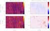 |
Fig. 17 Comparison of the properties of the residuals after denoising by our autoencoder (top) and ROHSA (bottom). The right column shows the map of the residual RMS, and the left column shows the map of the residual RMS normalized by the noise standard deviation. |
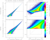 |
Fig. 18 Comparison of the denoising performances of the taylored autoencoder (top) and ROHSA (bottom). Each panel shows the joint histogram of the denoised intensities vs. the data intensities. The left and right columns display the full dynamic range of intensities and a zoom into the low intensities. A arcsinh transform was applied in order to show the intensities below 5σ (lower dashed square) with a linear scale and above 20σ with a logarithm scale (upper dashed square). The dotted line highlights the identity function. |
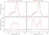 |
Fig. 19 Comparison of the spectral profiles and residuals for the autoencoder (left) and ROHSA (right) algorithms. Top: comparison of the input (in black) and output (in red) intensities. Bottom: comparison of the residuals between the input and denoised data. |
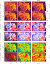 |
Fig. 20 Maps of the properties of the 13CO (1–0) line before (left) and after denoising with the autoencoder (middle) and ROHSA (right). From top to bottom, the properties are the maximum of the line, the line integrated intensity, the velocity of the maximum, the centroid velocity, a robust estimation of the line width, and the velocity dispersion. |
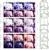 |
Fig. 21 Maps and histograms of the residuals of the properties of the 13CO (1−0) line. The properties are the same as for Fig. 20. The first, second, and third columns show the maps of residuals between the autoencoder denoised and raw data, the ROHSA denoised and raw data, and the ROHSA and autoencoder denoised data, respectively. The color scales are saturated in order to emphasize the differences where some signal is detected. The fourth column shows the associated histograms. The brown and green lines show the residuals from the autoencoder and ROHSA denoising, respectively. The black lines show the difference between the autoencoder and ROHSA results. |
8.3 Perspectives
Our autoencoder does not rely on the spatial information, in particular, the spatial correlations of the noise. Wavelet scattering transforms and wavelet phase harmonic transforms are recent tools that allow the spatial texture of data to be characterized in statistical ways with only a few hundred coefficients (Allys et al. 2019; Levrier et al. 2021). This can be used to denoise astrophysical data as proposed by Regaldo-Saint Blancard et al. (2020). Investigating whether this would improve the denoising performances achieved here will be the subject of a forthcoming paper.
9 Conclusion
In this paper, we have proposed a promising approach to denoise radio-astronomy line data cubes, inspired by a method developed to denoise hyperspectral cubes in Earth remote sensing. To do this, we first characterized in-depth the properties of the noise and signal for two radio-astronomy position-position-velocity cubes that are part of the ORION-B IRAM 30 m large program, namely the 13CO (1–0) and C17O (1–0) cubes.
The additive noise is well represented by a Gaussian random variable. Its RMS value varies spatially and spectrally. It can be modeled as the product of a spatial and a spectral contribution.
The spatial variations come from a combination of the source scanning strategy, variations of the atmospheric conditions between winter and summer runs, for example, and the source elevation during each observing session.
The spectral variations mostly have two origins. First, the resampling (currently) required to correct for Doppler effects in wide-bandwidth observations implies a sinusoidal oscillation of the noise level with frequency. Second, the interpolation of the polynomial fit of the baseline also slightly increases the noise RMS in the line frequency range.
The noise spatial power distribution can be modeled as the sum of two components: i) the square of the Fourier transform of the telescope point spread function, and ii) the modeling of the noise correlation introduced by sharing the same reference spectra among many on-source spectra.
The noise spectral autocorrelation can be modeled by the autocorrelation of a finite impulse response filter with a shape of [0.18 0.97 0.18]. This implies that the noise between pairs of channels is uncorrelated as long as their distance is larger than two channels.
Moreover, the signal is sparse along the spectral axis. This allows an easy estimation of the noise level and the associated S/N. This S/N varies from less than one to several hundred, mostly because of the large intensity dynamic range. The uncertainty budget is dominated by additive noise at a low S/N, but it becomes dominated by multiplicative noise due to the uncertain calibration when the S/N is larger than the inverse of the RMS of the calibration uncertainty: on the order of 20 in our case. For this study, we only denoised the low S/N part of the observations dominated by additive noise.
We then looked at the cube as a set of spectra that were individually denoised by dimension reduction. This method assumes that there is linear or nonlinear redundancy between the data features (here the channels of any spectrum). This hypothesis is well verified by standard hyperspectral cubes usually produced in Earth remote sensing. A mutual information computation shows that this hypothesis is more problematic for radio-astronomy line cubes, because the signal information decorrelates quickly from one channel to another at the obtained spectral resolution. From this viewpoint, denoising by dimension reduction would be more adapted to astronomy hyperspectral cubes observed with direct detection imaging spectrometers used to study the spectral energy distribution of the sources. When dealing with cubes that only contain spectrally resolved line emission, any denois-ing method by dimension reduction must thus take into account the fast decorrelation of channels that characterize these cubes.
An autoencoder is a nonlinear low rank deep learning denois-ing method whose goal is to minimize the distortion of the signal. We adapted the typical architecture to our line data as follows.
The proposed architecture took the fast decorrelation of the signal into account as a function of frequency.
We took the sparsity of the signal into account inside the spectrum by adapting the loss function of the autoencoder depending on whether the voxels contain mostly signal or mostly noise. This implies an a priori position-position-frequency classification algorithm.
For signal voxels, we weighed the distance between the data and the autoencoded data by the inverse of the noise variance. For noise voxels, we used the L1 norm between the autoencoded data and zero to ensure that the autoencoder would not create or destroy flux for low S/N voxels.
We finally compared the denoising performance to that achieved by the ROHSA algorithm that represents the spectra as a set of Gaussian fits. While ROHSA allows one to decompose the signal into velocity layers (e.g., Gaudel et al. 2023), the denoising performances of the proposed autoencoder are higher. The latter allowed us to increase the S/N in pixels with a low S/N while preserving the shape of spectra in high S/N pixels.
Acknowledgements
This work is based on observations carried out under project numbers 019-13, 022-14, 145-14, 122-15, 018-16, and finally the large program number 124-16 with the IRAM 30m telescope. IRAM is supported by INSU/CNRS (France), MPG (Germany) and IGN (Spain). This work was supported by the French Agence Nationale de la Recherche through the DAOISM grant ANR-21-CE31-0010, and by the Programme National “Physique et Chimie du Milieu Interstellaire” (PCMI) of CNRS/INSU with INC/INP, co-funded by CEA and CNES. This project also received financial support from the CNRS through the MITI interdisciplinary programs. J.R.G. and M.G.S.M. thank the Spanish MCINN for funding support under grant PID2019-106110G-100. Part of the research was carried out at the Jet Propulsion Laboratory, California Institute of Technology, under a contract with the National Aeronautics and Space Administration (80NM0018D0004). D.C.L. was supported by USRA through a grant for SOFIA Program 09-0015. We thank Antoine Marchal and Marc-Antoine Miville-Deschenes for their help in using the ROHSA algorithm. We thank the referee for valuable comments that helped us to improve the manuscript.
Appendix A Doppler effect and implied spectral resampling
The observed lines are emitted in the source frame at the line rest frequency, for example frest = 110.20135 GHz for the 13CO (1–0) line. The relative motion between the observatory and the Orion B molecular cloud in the Milky Way implies that the lines are recorded in the observatory frame at a frequency shifted by the Doppler effect. Pety & Bardeau (2011) describe in depth the consequences of this effect on the spectral data. In short, this effect can be approximated to first order in the Doppler parameter  (radio velocity convention) as
 (A.1)
(A.1)
where c is the speed of light, vsou/obs the component of the source velocity along the line of sight in the observatory frame, and fobs the observed frequency.
Moreover, the spectrum is regularly sampled in frequency. Its frequency axis is thus described as
 (A.2)
(A.2)
where ƒref is the reference frequency at the reference channel iref, and δ f the frequency channel spacing. The astronomer is interested by the description of the velocity variations in the source rest frame. However, the spectrum is recorded in the observatory frame. The same intensity I(i) of the spectrum can thus be attributed to two different frequencies, fobs(i) and frest(i). Equation A.2 can thus be written in the two frames for the same channel i as
 (A.3)
(A.3)
 (A.4)
(A.4)
Applying Eq. A.1 yields
 (A.5)
(A.5)
On one hand, the channel spacing in the observatory frame (δ fobs) is fixed by the spectrometer hardware. On the other hand, there is an infinite number of ( ) values to describe the same spectrum. The simplest choice is to set
  to the rest frequency of the line of interest, for example fest = 110.20135 GHz for the 13CO (1–0) line, and to use
  as the tuning frequency of the receiver, implying that the reference channel and thus the associated line will be localized at the middle of the spectrum frequency axis.
The Doppler frequency shift (frest – fobs) of Eq. A.1 varies with time during the day because of the Earth rotation around its axis and during the year because of the Earth rotation around the Sun. To remove this time dependency at the tuning frequency, radio-observatories slightly shift the tuning frequency with time according to the relative velocity between the observatory and the inertial frame, named Kinematic Local Standard of Rest (LSRK). The remaining Doppler effect between the LSRK frame and the source rest frame is dealt with in the data reduction software because it is independent of the observing time. However, the hardware correction, called real-time Doppler tracking, has two main limitations.
First, as it is only applied to the tuning frequency, it exactly corrects only the rest frequency at the reference channel while the radio-astronomy receivers observe wide bandwidth at high spectral resolution. The frequency scale in the source frame thus experiences a time-dependent frequency dilation around the reference frequency: δ frest = δ fobs/ {1 – vsou/obs(t/c}, with δ fobs the channel spacing fixed by the spectrometer hardware in the observatory frame. The order of magnitude of the Earth velocity in the LSRK frame, |Δv| ≤ 30 km s−1, implies that the dilation effect, δ frest, becomes on the order of the channel spacing every few tens of thousands channels. No observatory is yet proposing a hardware solution to correct for this dilation effect.
Second, when scanning the receiver over a portion of the sky to obtain wide-field imaging, the Doppler tracking correction is computed only once at the start of each scan. This is to ensure that potential standing wave associated with the cavity composed of, for example, the primary and secondary mirrors, have a periodicity along the frequency axis that is fixed during the scan duration. The Doppler tracking correction is thus only approximate because it is computed only once every few minutes in a particular sky direction, while the Doppler effect continuously depends both on the time and sky direction. The dependence on the sky direction is most problematic when scanning a wide portion of sky during a single scan.
Correcting for the time and space dependence of the Doppler effect implies a shift of the reference channel (iref) at constant reference frequency ( ) in the source frame (for details, see, e.g., Pety & Bardeau 2011). The observed spectra are thus slightly shifted in frequency. Moreover, current heterodyne receivers cover two frequency bands located below (lower side band) and above (upper side band) the frequency of the local oscillator. Due to the difference in frequency between the two bands (16 GHz for the EMIR receiver), the velocity scales are slightly different for these two side bands. Furthermore the separation of the signals from the two bands is not perfect. This may lead to the apparition of “ghost” lines from the rejected band at frequencies that depend on the local oscillator frequency. We refer the reader to Pety & Bardeau (2011) for associated details. All in all, the spectra thus need to be resampled to a common frequency axis before merging them to avoid blurring the spectral response in the science-ready product.
Appendix B Calibration in a nutshell
In this appendix, we summarize the calibration of the raw data, which combines the determination and application of the time varying calibration factor with the removal of the contribution of the atmosphere to the measured intensity. For simplicity, we start with assuming that the gain of the measurement is constant with time before generalizing to the case where the gain actually varies with time. We finally look at the impact of this calibration scheme on the measured noise. We do not speak about important additional subtleties, such as the impact of the mixing of the image sideband into the signal sideband or the usefulness of smoothing the frequency bandpass response when determining the calibration gain.
B.1 Time independent gain
The intensity measured (Imeas) by the receiver can be written before calibration and to zero order as the sum of the contribution of the astronomical signal (S astro) and of the atmospheric emission (S atm), multiplied by a gain (ɡ)
 (B.1)
(B.1)
The astronomer is interested to recover the astronomical signal. However, the contribution of the atmosphere most often completely dominates the astronomical signal at millimeter wavelengths, in other words Sastro ≪ Satm. It is thus required to measure independently the contribution of the atmosphere in order to subtract it. A common way to do this is to regularly observe a reference line of sight in between the observations of the on-source lines of sight. This method is called position switching. Writing the two observations as
 (B.2)
(B.2)
 (B.3)
(B.3)
this gives
 (B.4)
(B.4)
When the reference line of sight is actually devoid of signal ( ), and the contribution from the atmosphere is stable between the on-source and reference lines of sight, the last two terms cancel and we obtain
 (B.5)
(B.5)
B.2 Time varying gain
This gain is a combination of the absorption of the atmosphere and of the electronic amplification of the receiver. The electronic gain is constant over a typical timescale of about 30 minutes. But the atmosphere absorption varies on much shorter timescales. Moreover the atmosphere absorption and receiver amplification vary with frequency. In order to take into account the time variation of the system (atmosphere + receiver) gain, we model it as the product of the atmosphere and the receiver gain
 (B.6)
(B.6)
Using this expression in Eq. B.2 and B.3, we obtain
 (B.7)
(B.7)
 (B.8)
(B.8)
In order to solve for  , we first remove the receiver dependency because it dominates the spectral part of the gain variations, in particular at the edges of the observed bandpass. To do this, we just take the ratio of the ON and REF measurements. This yields
![Mathematical equation: ${{{\rm{ON}}} \over {{\rm{REF}}}} = {{g_{{\rm{on}}}^{{\rm{atm}}}} \over {g_{{\rm{ref}}}^{{\rm{atm}}}}}{{\left[ {S_{{\rm{on}}}^{{\rm{astro}}} + S_{{\rm{on}}}^{{\rm{atm}}}} \right]} \over {\left[ {S_{{\rm{ref}}}^{{\rm{astro}}} + S_{{\rm{ref}}}^{{\rm{atm}}}} \right]}}\~1.$](/articles/aa/full_html/2023/09/aa46064-23/aa46064-23-eq57.png) (B.9)
(B.9)
This ratio is of order 1 for two reasons
1 The astronomical signal is (most often) dominated by the atmospheric signal, in other words Sastro ≪ Satm.
2 The time variation of the gains are mostly due to variations of the atmosphere absorption, which are to first order anti-correlated with the variations of the atmosphere emission. This can be written as
 (B.10)
This is of course only true when the atmosphere varies only slightly during the observation.
We thus subtract 1 to the ratio of Eq. B.9 in order to mimic a Taylor decomposition. Solving for  then yields the sum of three terms
 (B.11)
 (B.12)
 (B.13)
 (B.14)
Equation B.11 is a generalization of Eq. B.4 to the case where the gain varies with time during the observations. Both have three terms.
The baseline The term ℬ is the residual that is nonzero when the assumption that the atmosphere emission and absorption are anticorrelated, that is Eq. B.10, breaks. This term is responsible for the typical continuum variations, called baselines, seen around the lines. These baseline offsets are removed through the baselining procedure described in Sect. 5.1.
The reference signal The term  is exactly zero, except when there exists some residual signal from the astronomical source on the reference line of sight. This happens for lines whose emission is extended over several degrees on the plane of sky, for instance, the 12CO and 13CO (1–0) emissions from local Giant Molecular Clouds. This is nevertheless rather the exception than the rule. When this term is nonzero, it can not be treated through baselining as the previous continuum offset. Indeed, it has a similar shape as the on-source line. It must thus be measured independently at relatively large signal-to-noise ratio and added back to the calibrated on-source signal. Contrary to common belief, this is
  that must be added, and not
  . In other words, the astronomical signal toward the reference line of sight must be added after multiplication by the time gain ratio between the on-source and reference observations.
The on-source signal Under perfect conditions, we recover an equation whose shape is similar to Eq. B.5, that is
 (B.15)
The term in parenthesis is unitless and the system temperature (Tsys) is the multiplicative calibration factor needed to establish the correct intensity unit scale. The system temperature depends both on frequency and time.
Appendix C Noise spatial power density
The spatial energy density of a 2D stochastic process D is defined as
![Mathematical equation: ${{\cal E}_D}\left( {u,\upsilon } \right) = {\rm{E}}\left[ {{{\left| {{\cal F}\left[ D \right]} \right|}^2}\left( {u,\upsilon } \right)} \right],$](/articles/aa/full_html/2023/09/aa46064-23/aa46064-23-eq68.png) (C.1)
(C.1)
where ℱ [D] is the Fourier transform of D, and E is the expectation operator. In our case, the stochastic process is the measurement of the signal affected by random noise over an image of area Aima, and the expectation is measured as the average of the images over a given number of channels. The spatial power density of D is then defined as the spatial energy density divided by the area of the image, that is
 (C.2)
(C.2)
The reference spectrum is observed only in between the observation of two consecutive lines on source. The integration time at the reference position is much larger than the one for each ON spectrum. The contribution of the noise from the reference position to the noise of the calibrated spectrum is thus negligible when computing the noise RMS per ON position. However, the noise of the reference spectrum is shared by all the ON spectra of two consecutive lines, implying a noise energy level correlated to the scanning configuration (rectangular patterns).
Here, we first compute the first order term of the Taylor decomposition of Eq. B.15 at point Satm. This allows us to show that the noise spatial power density is to first order the sum of two components coming from the ON and REF noise spatial behaviors, respectively. We finally compute the quantitative impact of the noise correlation introduced by the REF measurements.
C.1 Linearization of the measurement equation
We restart from Eq B.15 that relates the calibrated signal to the ON and REF measurements to show that we have to first order for channels devoid of signal
![Mathematical equation: $S_{{\rm{on}}}^{{\rm{astro}}}\left( {{\theta _l},{\theta _m},{\theta _{l0}},{\theta _{m0}}} \right) \simeq \left[ {B \star {N_{{\rm{on}}}}} \right]\left( {{\theta _l},{\theta _m}} \right) - \left[ {B \star {N_{{\rm{ref}}}}} \right]\left( {{\theta _{l0}},\theta { & _{m0}}} \right),$](/articles/aa/full_html/2023/09/aa46064-23/aa46064-23-eq70.png) (C.3)
(C.3)
where ⋆ is the convolution symbol, B is the point spread function of the telescope, and (Non, Nref) are a couple of centered normal random variables of same standard deviation as the atmospheric signal on source or on reference, respectively.
To do this, we first redefine the On and REF measurements to take into account three things. First, we compute the noise spatial power density only on channels devoid of line astronomical signal. In other words, we assume that Sastro = 0. Second, the coupling of the telescope to the sky is imperfect. This translates into a convolution equation. Third, the telescope is scanning the sky when observing on source, while it always comes back to the same position, (θl0, θm0), devoid of astronomical signal, when observing the reference. Given coordinates (θl, θm) and (θl0, θm0) at which ON and REF spectra are respectively measured, we obtain the measurement expressions
![Mathematical equation: ${\rm{ON}}\left( {{\theta _l},{\theta _m}} \right) = {g^{{\rm{rec}}}}g_{{\rm{on}}}^{{\rm{atm}}}.\left[ {B \star S_{{\rm{on}}}^{{\rm{atm}}}} \right]\left( {{\theta _l},{\theta _m}} \right),$](/articles/aa/full_html/2023/09/aa46064-23/aa46064-23-eq71.png) (C.4)
(C.4)
![Mathematical equation: ${\rm{REF}}\left( {{\theta _{l0}},{\theta _{m0}}} \right) = {g^{{\rm{rec}}}}g_{{\rm{ref}}}^{{\rm{atm}}}.\left[ {B \star S_{{\rm{ref}}}^{{\rm{atm}}}} \right]\left( {{\theta _{l0}},{\theta _{m0}}} \right).$](/articles/aa/full_html/2023/09/aa46064-23/aa46064-23-eq72.png) (C.5)
(C.5)
The atmospheric signal Satm can be considered as a normal random variable of expectation 𝔼 [Satm] and standard deviation σatm. As explained above σatm/𝔼 [Satm] ≪ 1 in millimeter radio-astronomy. In order to prepare to compute the Taylor decomposition of Eq. C.3 in 𝔼 [Satm], we rewrite the atmospheric random variable as
![Mathematical equation: $\matrix{ {{S^{{\rm{atm}}}} = \left[ {{S^{{\rm{atm}}}}} \right]\left( {1 + {\rm{\Delta }}} \right),} & {{\rm{with}}} & {{\rm{\Delta }} = {N \mathord{\left/ {\vphantom {N }} \right. \kern-\nulldelimiterspace} }\left[ {{S^{{\rm{atm}}}}} \right]} \cr } ,$](/articles/aa/full_html/2023/09/aa46064-23/aa46064-23-eq73.png) (C.6)
(C.6)
where δ is a centered normal random variable of standard deviation ≪ 1. Replacing the definitions C.6 in Eq. C.4 and C.5, and using the fact that the integral of B is equal to one, we yield
![Mathematical equation: ${{{\rm{ON}}\left( {{\theta _l},{\theta _m}} \right)} \over {{\rm{REF}}\left( {{\theta _{l0}},{\theta _{m0}}} \right)}} = {{g_{{\rm{on}}}^{{\rm{atm}}}\left[ {S_{{\rm{on}}}^{{\rm{atm}}}\left( {{\theta _l},{\theta _m}} \right)} \right]} \over {g_{{\rm{ref}}}^{{\rm{atm}}}\left[ {S_{{\rm{ref}}}^{{\rm{atm}}}\left( {{\theta _{l0}},{\theta _{m0}}} \right)} \right]}}\left\{ {{{1 + \left[ {B \star {{\rm{\Delta }}_{{\rm{on}}}}} \right]\left( {{\theta _l},{\theta _m}} \right)} \over {1 + \left[ {B \star {{\rm{\Delta }}_{{\rm{ref}}}}} \right]\left( {{\theta _{l0}},{\theta _{m0}}} \right)}}} \right\}.$](/articles/aa/full_html/2023/09/aa46064-23/aa46064-23-eq74.png)
Using again the fact that the first term of the product is of order 1, and keeping only the first order term in the Taylor decomposition of the second product term, we find
![Mathematical equation: ${{{\rm{ON}}\left( {{\theta _l},{\theta _m}} \right)} \over {{\rm{REF}}\left( {{\theta _{l0}},{\theta _{m0}}} \right)}} = - 1 \simeq \left[ {B \star {{\rm{\Delta }}_{{\rm{on}}}}} \right]\left( {{\theta _l},{\theta _m}} \right) - \left[ {B \star {{\rm{\Delta }}_{{\rm{ref}}}}} \right]\left( {{\theta _{l0}},{\theta _{m0}}} \right).$](/articles/aa/full_html/2023/09/aa46064-23/aa46064-23-eq75.png) (C.7)
(C.7)
We obtain Eq. C.3 by 1) replacing this equation in Eq. B.15, 2) using the definition of N in Eq. C.6, and 3) recognizing that Tsys ~ 𝔼 [Satm].
C.2 Normalization of the pixel variances
We plan to compute the spatial power density of  . Equation C.3 indicates that the measured signal is to first order the subtraction of two central normal random variables of standard deviation σon and σref. The standard deviation of
  is thus
 (C.8)
(C.8)
As the weather and the source elevation is varying during the observations, σ varies with times and thus with the position in the final map as shown on Fig. 6. Fortunately, the observing conditions can be considered constant between the observation on source and on reference. This implies that
 (C.9)
(C.9)
where dton and dtref are the integration time on source and on reference. We can thus compute the spatial power density of the ratio  to get rid of the noise variations due to the weather or the source elevation. This simplifies the interpretation of the result. From this point on, we keep the notation of Eq. C.3, and just note that the random variables Non and Nref have for standard deviation σon/σ and σref/σ.
C.3 Relative contributions from the ON and REF measurements
The spatial power density of the difference of two independent random processes is the sum of the spatial power density of each random process. We thus get
 (C.10)
with
![Mathematical equation: ${\cal P}{\;_{{\rm{on}}}}\left( {u,v} \right) = {{\left[ {{{\left| {{\cal F}\left[ {B \star {N_{{\rm{on}}}}} \right]} \right|}^2}\left( {u,v} \right)} \right]} \over {{A_{{\rm{ima}}}}}}$](/articles/aa/full_html/2023/09/aa46064-23/aa46064-23-eq82.png) (С.11)
(С.11)
![Mathematical equation: $ = {A_{{\rm{pix}}}}{\left( {{{{\sigma _{{\rm{on}}}}} \over \sigma }} \right)^2}{\left| {{\cal F}\left[ B \right]} \right|^2}\left( {u,v} \right),$](/articles/aa/full_html/2023/09/aa46064-23/aa46064-23-eq83.png) (C.12)
(C.12)
and
![Mathematical equation: ${\cal P}{\;_{{\rm{ref}}}}\left( {u,v} \right) = {{\left[ {{{\left| {{\cal F}\left[ {B \star {N_{{\rm{ref}}}}} \right]} \right|}^2}\left( {u,v} \right)} \right]} \over {{A_{{\rm{ima}}}}}}.$](/articles/aa/full_html/2023/09/aa46064-23/aa46064-23-eq84.png) (C.13)
(C.13)
The noise spatial power density of the on-source noise delivers the usual result, that is, it is proportional to the Fourier transform of the point spread function of the telescope. In the next section, we compute the noise spatial power density of the reference noise. In particular, it is not proportional to |ℱ [B]|2 (u, v) because the reference position is always observed at the same position on sky.
С.4 Quantitative impact of the noise correlation
We shall assume that all on-source pixels inside a rectangle of area Arect share the same reference spectrum, and that these rectangles form a chessboard pattern. The images are paved by nrect rectangles. The impact (R) of the reference observations on the observation procedure can be modeled by a convolution of a random dirac comb III with a 2D rectangular shape Π
![Mathematical equation: $R\left( {{\theta _l},{\theta _m}} \right) = \left[ {{\rm{\Pi }} \star {\rm{}}} \right]\left( {{\theta _l},{\theta _m}} \right),$](/articles/aa/full_html/2023/09/aa46064-23/aa46064-23-eq85.png) (C.14)
(C.14)
 (C.15)
and
 (C.16)
where к is the index of one rectangle over the chessboard, (θl,k, θm,k) the position of center of each rectangle, and Nk is the random variable associated with each measurement of the reference position. This random variable is assumed to be a normal variable 𝒩( ). The factor 1/ATect that appears in the definition C.16 ensures that the integral of the 2D rectangular shape Π is equal to 1 (unitless), and that all the energy of the stochastic process R is contained into the energy of the random comb function Ш. Figure C.l illustrates this decomposition in the 1D case. We now show that the noise spatial power density of the process R is
![Mathematical equation: ${\cal P}{\;_R}\left( {u,v} \right) = {\left[ {\sin {\rm{C}}\left( {{{{\rm{\Delta }}{\theta _l}u} \over \lambda }} \right)\sin {\rm{C}}\left( {{{{\rm{\Delta }}{\theta _m}v} \over \lambda }} \right)} \right]^2}{A_{{\rm{rect}}}}\left\langle {\sigma _k^2} \right\rangle ,$](/articles/aa/full_html/2023/09/aa46064-23/aa46064-23-eq89.png) (C.17)
(C.17)
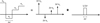 |
Fig. C.1 Illustration of the 1D calibration noise decomposition as the convolution between a random Dirac comb and a rectangular filter. |
where
 (C.18)
is the average of the noise variances of the reference measurements. Indeed, the properties of the Fourier transform and the deterministic nature of the Π function allow us to yield
![Mathematical equation: ${\cal P}{\;_R}\left( {u,v} \right) = {\left| {{\cal F}\left[ {\rm{\Pi }} \right]} \right|^2}\left( {u,v} \right){\cal P}{\;_{\rm{}}}\left( {u,v} \right).$](/articles/aa/full_html/2023/09/aa46064-23/aa46064-23-eq91.png) (C.19)
(C.19)
As the Fourier transform of a boxcar is a cardinal sine,
![Mathematical equation: ${\left| {{\cal F}\left[ {\rm{\Pi }} \right]} \right|^2}\left( {u,v} \right) = {\left[ {\sin {\rm{C}}\left( {{{{\rm{\Delta }}{\theta _l}u} \over \lambda }} \right)\sin {\rm{C}}\left( {{{{\rm{\Delta }}{\theta _m}v} \over \lambda }} \right)} \right]^2}.$](/articles/aa/full_html/2023/09/aa46064-23/aa46064-23-eq92.png) (C.20)
(C.20)
As III is a white noise, its energy spectral density is a constant. By using the energy conservation property of the Fourier transform, we get
![Mathematical equation: ${\cal P}{\;_{\rm{}}}\left( {u,v} \right) = {{A_{{\rm{rect}}}^2} \over {{A_{{\rm{Ima}}}}}}\sum\limits_{k = 1}^{{n_{{\rm{rect}}}}} {\left[ {N_k^2} \right]} .$](/articles/aa/full_html/2023/09/aa46064-23/aa46064-23-eq93.png) (C.21)
(C.21)
Finally, using Eq. C.18 and the fact that Aima = Аrect nrect, the spatial power distribution of the 2D random comb is
 (C.22)
Appendix D Calibration uncertainty
Fig. D.1: Relative variation of the fitted Gaussian area for the 13CO (1–0) line toward the Horsehead core in percentage. The left panel shows the variations as a function of the time of the measurements, while the right panel shows the histogram of the variations. The black and red colors are used for the H and V polarizations of the EMIR receiver. The vertical error bars around each point show the uncertainties on the fitted area due to thermal noise. The horizontal dashed lines show the mean variation for each polarization. The horizontal dotted lines show the ± 1σ level for all the measurements.
In order to monitor the calibration uncertainty, we observed the same position with known and bright line intensities at the start of each 8-hour block of observations. We choose the Horse-head core position (located at (+20″, +22″) from the projection center of 05h40m54.270s, −02º28′00.00″) as this position has been extensively studied in the framework of the Horsehead WHISPER survey (see, e.g., Guzmán et al. 2012; Pety et al. 2012; Gratier et al. 2013; Guzmán et al. 2013). We used the symmetric position switching observing mode with a reference position located at (−100″, 0″) from the projection center. We
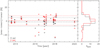 |
Fig. D.1 Relative variation of the fitted Gaussian area for the 13CO (1–0) line toward the Horsehead core in percentage. The left panel shows the variations as a function of the time of the measurements, while the right panel shows the histogram of the variations. The black and red colors are used for the H and V polarizations of the EMIR receiver. The vertical error bars around each point show the uncertainties on the fitted area due to thermal noise. The horizontal dashed lines show the mean variation for each polarization. The horizontal dotted lines show the ± 1σ level for all the measurements. |
In order to monitor the calibration uncertainty, we observed the same position with known and bright line intensities at the start of each 8-hour block of observations. We choose the Horse-head core position (located at (+20″, +22″) from the projection center of 05h40m54.270s, −02°28′00.00″) as this position has been extensively studied in the framework of the Horsehead WHISPER survey (see, e.g., Guzmán et al. 2012; Pety et al. 2012; Gratier et al. 2013; Guzmán et al. 2013). We used the symmetric position switching observing mode with a reference position located at (−100″, 0″) from the projection center. We integrated 6 minutes in total (3 minutes on source and 3 minutes on reference). This yields 55 measurements times two polarization spread over slightly more than 6 years and observed during varying weather conditions.
Calibration and reduction were done using standard methods of MRTCAL and CLASS. After extracting 11 MHz around the 13CO (1–0) rest frequency, we averaged the 110 separate spectra. The mean spectrum of all 110 measurements was fitted with a single Gaussian to get a reference value for the13 CO (1–0) line integrated intensity. In this fit, we only considered the main component of Orion B, near 10 km s−1. We then fit a single Gaussian for each 6-minutes measurement using the solution for the averaged spectra as initial guess for the fit and we visually checked that all fits were good. We then computed the variation of each measurement relative to the value derived for the average spectrum. Figure D.1 shows the relative variations as a function of the time and their histograms for the H and V EMIR polarizations separately.
The relative variations range from −25 to +10%. The vertical polarization delivers almost systematically a larger intensity than the horizontal polarization. This explains why the mean relative variations are +1.01 and −1.09%, respectively. The RMS around these means are 6.8 and 6.1%. The median absolute deviations are 5.0 and 4.3%, respectively. The difference between the RMS and median absolute deviation implies that a few measurements are outliers. Overall, the calibration uncertainty for the IRAM 30m is on the order of 5% for an almost instantaneous observation at 3 mm, as is the case for the ORION-B project. Averaging many such measurements when, for example, observing low brightness sources, considerably reduces this uncertainty. This experiment says nothing about the absolute calibration accuracy.
Appendix E About the multilayer perceptron
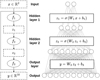 |
Fig. E.1 Example of graphical representation of a multilayer perceptron. The left part of the figure represents the network as a flowchart, highlighting the successive operations applied to the inputs. The right part shows the detailed architecture of the network, in this case consisting of two inputs, ten outputs and two hidden layers of four and height neurons, respectively. |
A neural network is a graphical model that maps nonlinearly outputs from inputs. A neural network architecture represents a given class of function. Neural networks are composed of a succession of layers that perform nonlinear transformations. Figure E.1 shows an example of a forward propagation architecture, named multilayer perceptron. Forward propagation means that the output of one layer is always the input of the next layer, while multilayer implies that there are at least two layers. In addition, the layers are fully connected, which means that each output of a layer is computed from all inputs. More precisely, for each layer, the input x and the output y are related through
 (E.1)
(E.1)
where W and b are respectively the weight matrix and the bias vector, which are estimated during the learning step. The biases enable one to shift the argument of a nonlinear activation function σ. Such a perceptron has the universal approximation property. It is able to approximate as precisely as required any continuous function provided it has enough neurons.
Appendix F A short introduction to mutual information
In information theory, mutual information is a quantity that measures the statistical dependence of two variables. The mutual information in base 2 of two continuous real variables X and Y is calculated as
 (F.1)
(F.1)
with fx, fY, and fX,Y respectively the probability density functions of X, Y, and (X, Y).
Mutual information is a positive real quantity and it is symmetric. In other words, I (X, Y) = I (Y, X). If there exists a function f (linear or not) such that Y = f (X), then I (X, Y) = +∞. Conversely, if the knowledge of one of the variables gives no information about the other (i.e., the two variables are independent) then I (X, Y) = 0. Mutual information is therefore a more general indicator than Pearson or Spearman correlation coefficient since it takes into account nonlinear and nonmonotonic relationships. In particular, it is possible for two variables to be decorrelated but have nonzero mutual information.
Appendix G Supplementary figures
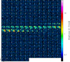 |
Fig. G.1 Visualization of the 240 spectral images of the 13CO (1–0) cube sorted by increasing velocity. |
References
- Allys, E., Levrier, F., Zhang, S., et al. 2019, A&A, 629, A115 [NASA ADS] [CrossRef] [EDP Sciences] [Google Scholar]
- Carter, M., Lazareff, B., Maier, D., et al. 2012, A&A, 538, A89 [NASA ADS] [CrossRef] [EDP Sciences] [Google Scholar]
- Duda, R. O., & Hart, P. E. 1973, Maximum Likelihood Estimation (New York: John Wiley and Sons, Inc.), 44 [Google Scholar]
- Ferré, L. 1995, Comput. Stat. Data Anal., 19, 669 [CrossRef] [Google Scholar]
- Gaudel, M., Orkisz, J. H., Gerin, M., et al. 2023, A&A, 670, A59 [NASA ADS] [CrossRef] [EDP Sciences] [Google Scholar]
- Gelfand, I. M., & Yaglom, A. 1959, Calculation of the Amount of Informationabout a Random Function Contained in Another Such Function (American Mathematical Society Providence) [Google Scholar]
- Gratier, P., Pety, J., Guzmán, V., et al. 2013, A&A, 557, A101 [CrossRef] [EDP Sciences] [Google Scholar]
- Gratier, P., Bron, E., Gerin, M., et al. 2017, A&A, 599, A100 [CrossRef] [EDP Sciences] [Google Scholar]
- Guzmán, V., Pety, J., Gratier, P., et al. 2012, A&A, 543, A1 [Google Scholar]
- Guzmán, V. V., Goicoechea, J. R., Pety, J., et al. 2013, A&A, 560, A73 [Google Scholar]
- Harshman, R. A. 1970, UCLA Working Papers in Phonetics, 16, 1 [Google Scholar]
- Hornik, K., Stinchcombe, M., & White, H. 1989, Neural Netw., 2, 359 [NASA ADS] [CrossRef] [Google Scholar]
- Kingma, D. P., & Ba, J. 2014, arXiv e-prints [arXiv: 1412.6988] [Google Scholar]
- Klein, B., Philipp, S. D., Güsten, R., Krämer, I., & Samtleben, D. 2006, SPIEConf. Ser., 6275, 627511 [NASA ADS] [Google Scholar]
- Klein, B., Hochgürtel, S., Krämer, I., et al. 2012, A&A, 542, A3 [Google Scholar]
- Kraskov, A., Stögbauer, H., & Grassberger, P. 2004, Phys. Rev. E, 69, 066138 [NASA ADS] [CrossRef] [Google Scholar]
- Leroy, A. K., Hughes, A., Liu, D., et al. 2021, ApJS, 255, 19 [NASA ADS] [CrossRef] [Google Scholar]
- Levrier, F., Allys, E., Régaldo-Saint Blancard, B., et al. 2021, in SF2A-2021:Proceedings of the Annual Meeting of the French Society of Astronomy and Astrophysics, eds. A. Siebert, A. Siebert, K. Baillié, et al., 91 [Google Scholar]
- Licciardi, G. A., & Chanussot, J. 2015, IEEE Geosci. Remote Sensing Lett., 12, 1228 [CrossRef] [Google Scholar]
- Licciardi, G., & Chanussot, J. 2018, Eur. J. Remote Sensing, 51, 375 [NASA ADS] [CrossRef] [Google Scholar]
- Mangum, J. G., Emerson, D. T., & Greisen, E. W. 2007, A&A, 474, 679 [NASA ADS] [CrossRef] [EDP Sciences] [Google Scholar]
- Marchal, A., Miville-Deschênes, M.-A., Orieux, F., et al. 2019, A&A, 626, A101 [NASA ADS] [CrossRef] [EDP Sciences] [Google Scholar]
- Orkisz, J. H., Pety, J., Gerin, M., et al. 2017, A&A, 599, A99 [NASA ADS] [CrossRef] [EDP Sciences] [Google Scholar]
- Orkisz, J. H., Peretto, N., Pety, J., et al. 2019, A&A, 624, A113 [NASA ADS] [CrossRef] [EDP Sciences] [Google Scholar]
- O’Shea, K., & Nash, R. 2015, arXiv e-prints [arXiv:1511.08458] [Google Scholar]
- Pety, J., & Bardeau, S. 2011, Description of the spectral axis handling in CLASS, Tech. rep., iRAM Memo 2011-4 [Google Scholar]
- Pety, J., & Falgarone, E. 2003, A&A, 412, 417 [NASA ADS] [CrossRef] [EDP Sciences] [Google Scholar]
- Pety, J., Gratier, P., Guzmán, V., et al. 2012, A&A, 548, A68 [NASA ADS] [CrossRef] [EDP Sciences] [Google Scholar]
- Pety, J., Guzmán, V. V., Orkisz, J. H., et al. 2017, A&A, 599, A98 [NASA ADS] [CrossRef] [EDP Sciences] [Google Scholar]
- Pety, J., Gerin, M., Bron, E., et al. 2022, in European Physical Journal Web ofConferences, 265, 00048 [NASA ADS] [CrossRef] [EDP Sciences] [Google Scholar]
- Pilbratt, G. L., Riedinger, J. R., Passvogel, T., et al. 2010, A&A, 518, A1 [NASA ADS] [CrossRef] [EDP Sciences] [Google Scholar]
- Refaeilzadeh, P., Tang, L., & Liu, H. 2009, Encyclop. Database Syst., 5, 532 [CrossRef] [Google Scholar]
- Regaldo-Saint Blancard, B., Levrier, F., Allys, E., Bellomi, E., & Boulanger, F. 2020, A&A, 642, A217 [EDP Sciences] [Google Scholar]
- Riener, M., Kainulainen, J., Henshaw, J. D., et al. 2019, A&A, 628, A78 [NASA ADS] [CrossRef] [EDP Sciences] [Google Scholar]
- Rigby, J., Perrin, M., McElwain, M., et al. 2023, PASP, 135, id.048001 [Google Scholar]
- Rosolowsky, E., & Leroy, A. 2006, PASP, 118, 590 [NASA ADS] [CrossRef] [Google Scholar]
- Schölkopf, B., Smola, A., & Müller, K.-R. 1997, in International Conference on Artificial Neural Networks, Springer, 583 [Google Scholar]
- Shalev-Shwartz, S., & Ben-David, S. 2014, Understanding Machine Learning:From Theory to Algorithms (Cambridge University Press) [CrossRef] [Google Scholar]
- Vogel, C. R., & Oman, M. E. 1996, SIAM J. Sci. Comput., 17, 227 [CrossRef] [MathSciNet] [Google Scholar]
- Wold, S., Esbensen, K., & Geladi, P. 1987, Chemom. Intell. Lab. Syst., 2, 37 [CrossRef] [Google Scholar]
It is available on the IRAM large program archive at https://oms.iram.fr/?dms=frontpage
These cubes are available on the ORION-B project web page at https://www.iram.fr/~pety/ORION-B/data.html
To be precise, we could use the complete formulation, noise spatial and spectral power spectral density. This however introduces a confusion between the spectral (frequency, wavelength, or velocity) axis of astronomy cubes and the spectral density that refers to computations in the Fourier plane. We thus choose to remove spectral in power spectral density.
The latter dataset, named Indian Pines, has been acquired with the Airborne Visible/Infrared Imaging Spectrometer (AVIRIS) sensor over an agricultural area located at northwestern Indiana, USA. This cube is composed of 220 spectral channels ranging from 400 nm to 2500 nm. Its spatial linear resolution is 20 × 20 m. It is publicly available here https://www.ehu.eus/ccwintco/index.php/ Hyperspectral_Remote_Sensing_Scenes
Unlike a dense layer used in a perceptron which is composed of a matrix product, a convolutional layer is composed of a linear filter.
The Lq norm of the vector X = (x1,…,xn) is defined as  .
.
We also compared with the GAUSSPY+ algorithm (Riener et al. 2019), which guesses the number of fitted Gaussian components per pixels instead of fixing it over the full field of view as ROHSA does. While both algorithms deliver solutions with slightly different systematic deviations, the differences are not compelling enough to warrant presenting both of them.
The GILDAS software are distributed here https://www.iram.fr/IRAMFR/GILDAS/
All Tables
All Figures
|
Fig. 1 Comparison of mean intensity images between two radio-astronomy lines. |
| In the text | |
|
Fig. 2 Comparison of intensity spectra between the two radio-astronomy lines. The spectra show the mean (top), minimum and maximum (bottom) intensity as a function of the channel velocity or number. The vertical dashed red lines show the channels whose spatial distribution is plotted on Fig. 4. The vertical dotted lines on the radio-astronomy spectra separate the signal channels from the noise-only ones. |
| In the text | |
|
Fig. 3 Comparison of the histograms of the intensity of the two radio-astronomy lines. The left column shows the full intensity dynamical range, while the right column zoom on faint intensity. The black histogram is computed over all the data channels. The red and green histograms are computed over the channel ranges that contains either mostly noise or high signal-to-noise ratio intensity, respectively. |
| In the text | |
|
Fig. 4 Velocity channels at 6 and 10 km s−1 of 13CO (1–0). The corresponding channels are displayed as vertical dashed red lines in Fig. 2. |
| In the text | |
|
Fig. 5 Amount of information shared between channels for the 13CO(1–0) data cube. The top row shows information related only to linear relationship, while the bottom row shows information related to any type of relation (i.e., the mutual information). |
| In the text | |
|
Fig. 6 Noise spatial (top) and spectral (bottom) variations for the C17O (1–0) line cube. The spatial maps were normalized by the median noise value. The red region in the bottom panels shows the 3σ uncertainty interval of the computation. |
| In the text | |
|
Fig. 7 Comparison between the measured (left) and modeled (middle) noise spatial power density, and their ratios (right) in logarithmic scale. The top row shows the spatial power densities for all scales, while the bottom row zooms in on the large spatial scales. |
| In the text | |
|
Fig. 8 Comparison between the measured (plain line) and modeled (dashed line) spectral power density (left) and autocorrelation function (right). |
| In the text | |
|
Fig. 9 Example of an autoencoder neural network. Each column represents a neuron layer. Each arrow represents a connection between the neuron layers. The first and last layers are composed from the measured and denoised intensities of a spectrum at the different channels, respectively. The bottleneck contains the minimum number of neurons needed to compress the data without loss of signal information. In this example, the signal intrinsic dimension (size of the bottleneck) is three while the data extrinsic one (size of the input and output spectra) is 10. |
| In the text | |
|
Fig. 10 Distance (mean absolute deviation) between input and reconstructed data as a function of the bottleneck size for the 13CO (1–0) data (left) and the Indian Pines data (right). |
| In the text | |
|
Fig. 11 Illustration of the non-invariance to rotation of the L1 norm as opposed to the L2 norm. |
| In the text | |
|
Fig. 12 Optimized autoencoder architecture (a) where fully connected layers (b) are replaced by locally connected layers (c). The number of entries is 5 and the bottleneck is size 3. The hidden layers of the network can be described by describing the small encoders, here they are of dimension [3, 2] with input and output windows of the same size 3. |
| In the text | |
|
Fig. 13 Maps of the maximum (top) and minimum (bottom) S/N per spectrum before (left) and after (right) convolution of the C17O (1–0) line cube by the telescope point spread function. |
| In the text | |
|
Fig. 14 Properties of the segments obtained on the cube of S/N for the C17O (1–0) line. This cube was segmented into contiguous position-position-velocity regions above a minimum S/N value. The segments are ordered by decreasing value of the S/N summed over the segment (total S/N). The shown properties are, from top to bottom, the total number of pixels inside the segment, the total S/N, and the mean S/N of the segment. These properties are shown for two different S/N thresholds: 1 and 2. The blue plain vertical lines show the segments that are selected to compute the moment maps in Fig. 15. The red dashed horizontal lines show the typical mean S/N reached for the segment # 200. |
| In the text | |
|
Fig. 15 Maps of the moments of the spectrum for two different values (1 at left, and 2 at right) of the S/N threshold used to compute the position– position–velocity mask of significant emission. From top to bottom, the peak intensity (maximum of the spectrum), line integrated intensity (moment 0 of the spectrum), and centroid velocity (moment 1 of the spectrum) are shown. |
| In the text | |
|
Fig. 16 Comparison of the denoising performances of the taylored autoencoder and ROHSA for four different velocity channels belonging to the line wings. For each channel, the raw (left) and denoised (middle) images are shown with the same intensity scale and the residual (right) image is displayed with an optimized intensity scale. The top and bottom rows show the results for the autoencoder and ROHSA algorithms, respectively. |
| In the text | |
|
Fig. 17 Comparison of the properties of the residuals after denoising by our autoencoder (top) and ROHSA (bottom). The right column shows the map of the residual RMS, and the left column shows the map of the residual RMS normalized by the noise standard deviation. |
| In the text | |
|
Fig. 18 Comparison of the denoising performances of the taylored autoencoder (top) and ROHSA (bottom). Each panel shows the joint histogram of the denoised intensities vs. the data intensities. The left and right columns display the full dynamic range of intensities and a zoom into the low intensities. A arcsinh transform was applied in order to show the intensities below 5σ (lower dashed square) with a linear scale and above 20σ with a logarithm scale (upper dashed square). The dotted line highlights the identity function. |
| In the text | |
|
Fig. 19 Comparison of the spectral profiles and residuals for the autoencoder (left) and ROHSA (right) algorithms. Top: comparison of the input (in black) and output (in red) intensities. Bottom: comparison of the residuals between the input and denoised data. |
| In the text | |
|
Fig. 20 Maps of the properties of the 13CO (1–0) line before (left) and after denoising with the autoencoder (middle) and ROHSA (right). From top to bottom, the properties are the maximum of the line, the line integrated intensity, the velocity of the maximum, the centroid velocity, a robust estimation of the line width, and the velocity dispersion. |
| In the text | |
|
Fig. 21 Maps and histograms of the residuals of the properties of the 13CO (1−0) line. The properties are the same as for Fig. 20. The first, second, and third columns show the maps of residuals between the autoencoder denoised and raw data, the ROHSA denoised and raw data, and the ROHSA and autoencoder denoised data, respectively. The color scales are saturated in order to emphasize the differences where some signal is detected. The fourth column shows the associated histograms. The brown and green lines show the residuals from the autoencoder and ROHSA denoising, respectively. The black lines show the difference between the autoencoder and ROHSA results. |
| In the text | |
|
Fig. C.1 Illustration of the 1D calibration noise decomposition as the convolution between a random Dirac comb and a rectangular filter. |
| In the text | |
|
Fig. D.1 Relative variation of the fitted Gaussian area for the 13CO (1–0) line toward the Horsehead core in percentage. The left panel shows the variations as a function of the time of the measurements, while the right panel shows the histogram of the variations. The black and red colors are used for the H and V polarizations of the EMIR receiver. The vertical error bars around each point show the uncertainties on the fitted area due to thermal noise. The horizontal dashed lines show the mean variation for each polarization. The horizontal dotted lines show the ± 1σ level for all the measurements. |
| In the text | |
|
Fig. E.1 Example of graphical representation of a multilayer perceptron. The left part of the figure represents the network as a flowchart, highlighting the successive operations applied to the inputs. The right part shows the detailed architecture of the network, in this case consisting of two inputs, ten outputs and two hidden layers of four and height neurons, respectively. |
| In the text | |
|
Fig. G.1 Visualization of the 240 spectral images of the 13CO (1–0) cube sorted by increasing velocity. |
| In the text | |
Current usage metrics show cumulative count of Article Views (full-text article views including HTML views, PDF and ePub downloads, according to the available data) and Abstracts Views on Vision4Press platform.
Data correspond to usage on the plateform after 2015. The current usage metrics is available 48-96 hours after online publication and is updated daily on week days.
Initial download of the metrics may take a while.