| Issue |
A&A
Volume 671, March 2023
|
|
|---|---|---|
| Article Number | A39 | |
| Number of page(s) | 13 | |
| Section | Numerical methods and codes | |
| DOI | https://doi.org/10.1051/0004-6361/202245139 | |
| Published online | 03 March 2023 | |
Utilization of convolutional neural networks for H I source finding
Team FORSKA-Sweden approach to SKA Data Challenge 2
1
Fraunhofer-Chalmers Centre & Fraunhofer Center for Machine Learning,
412 88,
Gothenburg,
Sweden
e-mail: This email address is being protected from spambots. You need JavaScript enabled to view it.
2
Department of Space, Earth and Environment, Chalmers University of Technology,
Onsala Space Observatory,
439 92
Onsala,
Sweden
e-mail: This email address is being protected from spambots. You need JavaScript enabled to view it.
Received:
5
October
2022
Accepted:
17
January
2023
Abstract
Context. The future deployment of the Square Kilometer Array (SKA) will lead to a massive influx of astronomical data and the automatic detection and characterization of sources will therefore prove crucial in utilizing its full potential.
Aims. We examine how existing astronomical knowledge and tools can be utilized in a machine learning-based pipeline to find 3D spectral line sources.
Methods. We present a source-finding pipeline designed to detect 21-cm emission from galaxies that provides the second-best submission of SKA Science Data Challenge 2. The first pipeline step was galaxy segmentation, which consisted of a convolutional neural network (CNN) that took an H I cube as input and output a binary mask to separate galaxy and background voxels. The CNN was trained to output a target mask algorithmically constructed from the underlying source catalog of the simulation. For each source in the catalog, its listed properties were used to mask the voxels in its neighborhood that capture plausible signal distributions of the galaxy. To make the training more efficient, regions containing galaxies were oversampled compared to the background regions. In the subsequent source characterization step, the final source catalog was generated by the merging and dilation modules of the existing source-finding software SOFIA, and some complementary calculations, with the CNN-generated mask as input. To cope with the large size of H I cubes while also allowing for deployment on various computational resources, the pipeline was implemented with flexible and configurable memory usage.
Results. We show that once the segmentation CNN has been trained, the performance can be fine-tuned by adjusting the parameters involved in producing the catalog from the mask. Using different sets of parameter values offers a trade-off between completeness and reliability.
Key words: methods: data analysis / methods: statistical / radio lines: galaxies
© The Authors 2023
 Open Access article, published by EDP Sciences, under the terms of the Creative Commons Attribution License (https://creativecommons.org/licenses/by/4.0), which permits unrestricted use, distribution, and reproduction in any medium, provided the original work is properly cited.
This article is published in open access under the Subscribe to Open model. This email address is being protected from spambots. You need JavaScript enabled to view it. to support open access publication.
1 Introduction
Designing robust strategies to find sources and build catalogs is key for the success of modern large astronomical surveys. Attempts to automatize the identification and characterization of astronomical sources are as old as the astronomical catalogs themselves and have evolved to our day by taking advantage of both technological progress and human intervention (e.g., from the works of the Harvard Computers, Nelson 2008, to the successful series of citizen science projects of Galaxy Zoo, Masters & Galaxy Zoo Team 2020). With the advent of massive data and the possibilities of automation, machine learning techniques are a tool with great potential in making astronomical discoveries.
Among the facilities that will become a reality in the next years in the field of astronomy, the future Square Kilometer Array (SKA) will catalyze a revolution in this area of research by tracing the 21-cm line emission of the neutral hydrogen (H I) atom back to the early Universe, thus enabling the study of the formation of its first galaxies (e.g., see chapter The Hydrogen Universe in Braun et al. 2015). This scientific revolution will come accompanied by many developments to face the challenge of processing the largest astronomical data sets to be produced in human history so far. That includes the need to automatize the search and characterization of the signal from massive quantities of galaxies in the observations delivered by SKA.
The field is quickly developing to address these future challenges and in this context, the SKA Observatory has initiated a series of “data challenges” to encourage the scientific community to specifically prepare for SKA. After a first challenge in 2018 aimed at detecting sources in a simulation of the radio continuum to be observed by SKA (Bonaldi et al. 2021), SKA Data Challenge 2 (SDC2) consisted of expanding the exercise to detect H I line sources in large 3D data cubes emulating the ones to be produced by the telescope in the near future (Hartley et al., in preparation). In this paper, we present and analyze the pipeline developed by our team FORSKA-Sweden, which scored the second-best submission in SDC2.
Historically, since the discovery of the 21-cm H I line in 1944 (van de Hulst 1945) and the construction of the first radio telescopes, the field of extragalactic H I science has had a long tradition of carrying out large surveys with telescopes around the globe (see e.g., Giovanelli & Haynes 2015, for a review), developing source detection and characterization techniques for 2D spectra and 3D data cubes, and finding the best proxies to study the physical properties of galaxies from the observational data. Some recent examples of algorithms for source detection that have paved the way to our work include, for instance, Serra et al. (2015); Whiting (2012); Westmeier et al. (2021); Whiting & Humphreys (2012). Former approaches have mainly relied on classical signal processing strategies to find extragalactic H I sources, and incorporating machine learning techniques is a natural step forward in the automation process.
Deep learning with convolutional neural networks (CNN) has been utilized extensively as an artificial intelligence technique within image recognition. Alongside impressive empirical results when applying CNNs in different application fields, their success can also be attributed to their specific adaptability to complex tasks with relatively little domain knowledge needed (LeCun et al. 2015). In addition, CNNs have been applied in radio astronomy (e.g., Lukic et al. 2018; González et al. 2018), including as algorithms presented to the first SKA Data Challenge aimed at detecting continuum sources (e.g., Lukic et al. 2019). Given the type of data generally involved in spectral line observations with radio interferometers that are primarily identifying coherent signal in 3D data cubes and the nature of the challenge with access to an ideal catalog of sources, we built our pipeline around supervised binary segmentation using CNNs. Binary segmentation is the general problem of separating an object of interest, in our case a galaxy, from the background in an image or similar (Thoma 2016; Liu et al. 2018). Recently, CNNs have become a popular approach for such problems when applied in other areas, such as medical imaging (Minaee et al. 2021). We used a general-purpose segmentation CNN, called u-net (Ronneberger et al. 2015), to generate a binary mask resembling the galaxy shape suggested by the true source catalog. To estimate the source characteristics, we took advantage of existing public code in SOFIA (Serra et al. 2015) for robust H I parameter estimation from the CNN-generated mask.
Our CNN-based solution and algorithms of the other competing teams in the challenge altogether set a good basis for source detection and characterization algorithms for SKA surveys in the future. In this paper, we give a thorough description and motivation of our pipeline, together with an analysis on how the pipeline can be tweaked to give a range in terms of performance. All code related to this project is publicly available at GitHub1. The SKA Data Challenge 2 general analysis and results for all teams will be presented un an upcomping work (Hartley et al., in prep.).
This paper is organized as follows: our methods for implementing the pipeline are presented in Sect. 2, an analysis of the performance is given in Sect. 3, followed by a discussion in Sect. 4 and our conclusions in Sect. 5.
2 Methods
The challenge data set consisted of a simulated H I data cube, its companion continuum data cube, and the catalog of sources that had been fed into the simulated H I data cube. The ultimate goal was to recover the latter catalog from the SKA data cubes. Given the challenge score definition, and the low chances of alignment of continuum sources with H I sources in the challenge cube, we did not search for absorption features and, therefore, we did not make use of the continuum data cube in our pipeline.
Our pipeline combines different disciplines by decomposing the overall problem of source catalog generation into the machine learning task of obtaining a source mask from the H I data cube through segmentation, followed by the astronomically focused source characterization given such a mask. Our method relies on supervised learning, which was possible to implement as the true source catalog for a simulated H I data cube was provided in the challenge. In many cases, we could take advantage of publicly available software, such as machine learning frameworks for segmentation and the domain-specific spectroscopic source-finding software SOFIA. However, to overcome computer memory limitations when applying our method and ensure its portability to different computing environments, we implemented an extra configuration layer that allows for its memory usage to be adjusted.
This section is structured as follows: in Sect. 2.1, we give a brief description of the simulated data we used, in Sect. 2.2, we formulate the segmentation problem of mask generation and give the machine learning-related details, in Sect. 2.3, we explain how the source characteristics were estimated from a mask, and in Sect. 2.4, we describe the considerations we had to take into account in the pipeline implementation to allow for flexible memory usage.
2.1 Data
All the development and evaluation of this work was based on the simulated data provided in SDC2. This data set consisted of a simulation of the Universe in the redshift interval z = 0.235−0.495, as observed by SKA in the frequency range of 950−1150 MHz. A description of the simulation was provided by the organizers2 and will be presented in an upcoming research paper (Hartley et al., in prep.). Here, we only summarize the data set to highlight the aspects that are relevant to presenting our method.
The simulated data set was the output of two layers of simulations. First, a putative representation of the galaxies inhabiting the Universe at those redshifts was generated in the form of a source catalog of galaxies with physical properties spanning the parameter space deemed realistic according to our current knowledge of galaxy formation and evolution. This catalog listing source positions and properties will be referred to as the true source catalog. Next, a simulation was run and produced a final H I data cube that mimics a 2000-h observation using SKA of the underlying true catalog of galaxies.
The attributes included in the source catalog (summarized in Table 1) are: source position (spatial coordinates of the galaxy center in the sky and central frequency) and source property characterization (integrated H I line flux, H I major axis, H I linewidth, disk position angle, and inclination). The H I line width corresponds to the observed width at 20% of its peak. The disk position angle was defined as the angle of the major axis of the receding side of the galaxy and inclination was defined as the angle between a normal to the galaxy disk and the line of sight. Also, the minor axis s could be retrieved from the source catalog from the equation:
 (1)
(1)
as suggested by an ellipsoidal shape of the galaxy with the ratio a between the thickness and S. For all simulated sources, α = 0.2 was used.
There were two simulated H I cubes: the development cube of 40 GB and the challenge cube of 850 GB. The first was provided to participants to develop their techniques, and thus when the challenge was still running, the true source catalog of the development cube was accessible for participants while the source catalog of the challenge cube was hidden. However, after the challenge was finished, also the source catalog of the challenge cube has been released to the public. As illustrated by the flowchart in Fig. 1, we used 80% of the development cube for training a segmentation model and the remaining 20% for validation, which is described in Sect. 2.2. After training the segmentation model, we used it in the pipeline and evaluated the performance, as described in Sect. 3, for a 40 GB sub-region of the challenge cube.
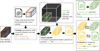 |
Fig. 1 Flowchart for data usage. Generating a mask from a true source catalog refers to the procedure presented in Sect. 2.2.2 and training step is described in Sect. 2.2.3. Pipeline employment covers both steps of galaxy segmentation (Sect. 2.2) and source characterization (Sect. 2.3). The evaluation refers to the analysis performed in Sect. 3. |
Source attributes in the catalog.
2.2 Step I: Galaxy segmentation
The purpose of the machine learning-oriented galaxy segmentation step was to detect galaxies and provide a mask to use for source characterization. On a high level, the mask output from this step can be viewed as a translation layer between machine learning and astronomy. From this perspective, we reasoned that the mask should be a representation of detected galaxies easing the source characterization. Our approach to obtaining such a mask was to inform training in the segmentation step. By making astronomical assumptions and based on the source properties given in the catalog, we constructed the target mask to be learned by the segmentation u-net. With access to the true source catalog, we could formulate the mask generation from the H I cube as supervised binary segmentation. Training a segmentation model in a supervised manner involves a target mask with the same shape as the input data, which the model is trained to output. In Sect. 2.2.1, we describe the segmentation CNN, in Sect. 2.2.2 we motivate the shape of the target mask, and in Sect. 2.2.3 we give all the details on how training was performed.
2.2.1 Segmentation model
Our segmentation model was a 3D u-net, which is a type of CNN specifically designed for segmentation. It was originally intended for two-dimensional (2D) biomedical segmentation (Ronneberger et al. 2015), but later also adapted to three-dimensional (3D) volumetric segmentation (Çiçek et al. 2016). The u-net architecture consists of two parts: the encoder and the decoder. In the encoder, convolutional layers are alternated with down-sampling layers, producing a hierarchy where low levels capture rough features occupying large space. For each of the resolution levels produced by the encoder, except the last, the decoder concatenates its output with the output from the earlier decoder level but upsampled. To produce the decoder-level output, further convolutional layers are applied to the concatenated tensor. The output of the final decoder layer is an image with the same shape as the input image. One benefit of the u-net architecture is that it is a fully convolutional neural network and therefore the input can be of almost any size. For example, in a setting with no memory restriction, we could propagate the whole cube through the model once, without the need for cropping into subcubes.
We used a model architecture provided by the Segmentation Models package (Yakubovskiy 2020) but modified it to handle 3D data, which is depicted in Fig. 2. Between each downsampling of the encoder, there was a sequence of multiple ResNet blocks, as described by He et al. (2016), but with batch normalization (Ioffe & Szegedy 2015) layers before each activation. Downsampling was performed into five different resolutions, lower than the original input, by striding a filter with a stride of 2. The upsampling in the decoder was done by linear interpolation. The convolution layers on each level of the decoder consisted of a double repetition of the sequence: convolution layer, batch normalization layer, and ReLU (Glorot et al. 2011) activation. The exception was for the last decoder layer, where a Sigmoid activation was used, meaning that all output values were between 0 and 1, as required for our target mask. As in the adaptation of u-net for volumetric data, we used 3D convolutions with every filter shaped as 3 × 3 × 3 voxels.
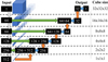 |
Fig. 2 Overview of the used u-net segmentation model for an example input cube of size 32 × 32 × 32. The encoder is formed by all grey vertical arrows pointing downwards on the plot, while the decoder consists of the remaining arrows on the right of the plot. The dashed lines separate the different resolutions, meaning that down- or upsampling actions are used to go between these. Black rectangles with numbers indicate the number of filters of the different stages. Gray arrows represent one or multiple ResNet blocks, each with one downsampling layer. Orange arrows represent upsampling layers, green represents copy and merger actions, and blue arrows represent a sequence of two decoder blocks. |
2.2.2 Target mask
To train our segmentation model, a target mask had to be constructed. This target mask should represent the shape suggested by the attributes provided in the true source catalog, that is, the attributes of line width, major axis, position angle, and inclination. Ignoring the voxel resolution of the mask, a mask constructed with this approach could perfectly reproduce the shape-related attributes of the source characterization procedures. Hence, our hope was that masks obtained from a segmentation CNN trained with these targets would attain a similar structure so that no handling of noise and blur needs to be involved in the source characterization. Analogous to deep learning applied for denoising problems (Tian et al. 2020), training should proceed easier if the mask resembles the galaxy regions in the H I cube. Therefore, we based the construction of the target mask on computing bounds on the line-of-sight velocity from basic astronomic assumptions applied to the shape-related attributes. However, the presence of blur introduces discrepancies between the shape as suggested by the source catalog and its appearance in the H I cube. To mitigate this and achieve more resemblance between the target mask and the data, we added extra padding to the target mask constructed from the astronomical assumptions.
For reference, all notation of source attributes introduced in this section is summarized in Table 1. Essentially, to compute the mask we assumed a simplistic model of a galaxy shaped as a circular disk with an infinitesimal thickness, where the orbital speed is a function of the radius. Consequently, the maximum orbital speed is upper bounded by  . Influenced by observed velocity profiles, for example, in De Blok et al. (2008), we also assumed a lower bound on the orbital speed so that the orbital period for any inner ring is at most the period at the disk’s boundary. Furthermore, we assumed the largest orbital speed at the disk’s boundary. When generating a mask based on these assumptions, we defined the ellipse shape by using the major axis, S, inclination, i, and position angle, θ, from the true source catalog together with the minor axis, s, calculated according to Eq. (1). For each pixel x, y, relative to the center and with a major axis aligned in the x-axis, inside the ellipse, the mask occupation was given by the inequalities:
 (2a)
(2a)
 (2b)
(2b)
where vC is the central velocity corresponding to the central frequency vc in Table 1 and
 (3)
(3)
A precise derivation of Eqs. (2a) and (2b) is given in Appendix A. A detailed description about the added padding to the mask that compensates for blur in the data can be found in Appendix B. Although this mask construction is obviously limited and potentially inaccurate, we assessed by visual inspection (exemplified in Fig. 3) that the resulting masks overlap with the most apparent features of the galaxies.
2.2.3 Training the segmentation CNN
Training the segmentation CNN was performed by minimizing a loss function of the CNN output and the target mask. Due to the nature of the data, we had to cope with a large data size and a severe class imbalance in the segmentation problem. To address these issues, we sample small sub-cubes from the development H I cube, allowing for an adjustment of both the size of the training data and the balance between the galaxy and background voxels.
It has been noted that the loss function used when training may play a significant role in the performance, but what is an appropriate choice may depend on the nature of the problem (Jadon 2020). As in the case of many other segmentation applications, the galaxy segmentation problem is highly imbalanced, so that the number of background voxels is remarkably larger than the number of galaxy voxels. Two common examples of segmentation loss functions are cross-entropy and soft Dice (Milletari et al. 2016), where the latter has often been preferred in more recent works with imbalanced classes (Bertels et al. 2019). However, it has also been noted that soft Dice makes training more unstable compared to cross-entropy (Nordström et al. 2020). When training the segmentation CNN, we used a linear combination of cross-entropy and soft Dice, which has been suggested as an attempt to alleviate such training instability (Taghanaki et al. 2019; Isensee et al. 2018). Hence, for N voxels predicted by the CNN, each of these denoted ŷi, i ∈ {1,…, N}, with corresponding target value yi, the loss function used was:
 (4)
(4)
To minimize this loss, we used the Adam optimizer (Kingma & Ba 2014), and repeatedly saved the models that achieved the smallest validation loss. The progress of the training and validation loss is viewed in Fig. C.1
In order to enable training on machines with different memory constraints and independent of the input H I cube size, we sampled sub-regions from the development cube, illustrated by the blue arrows in Fig. 4. For each source in the true source catalog, a galaxy container cube, that covered the corresponding mask and a padding of 32 voxels were generated. Also, background training cubes, of size 32 × 32 × 32, were sampled randomly from other regions with no galaxies present. Due to memory constraints, we set the number of background training cubes to four times the number of galaxy training cubes. By modifying this number, the data size could be adjusted to fit the machine on which the training was performed. The training data set consisted of the galaxy sub-cubes and background training cubes, together with their corresponding masks.
When creating batches used for training the segmentation CNN, we sampled background and galaxy training cubes, as illustrated by the orange arrows in Fig. 4. Background training cubes were randomly selected from the set of stored cubes, while galaxy training cubes were sampled from the galaxy container cubes. This semi-random sampling enabled tuning the ratio between galaxy and background in the training by simply adjusting the number of training cubes of each type.
We used a total batch size of 128 subcubes and evaluated the loss in Eq. (4) over the whole batch, that is, N = 128 · 32 · 32 · 32. The training cubes, together with the corresponding target cube, were rotated and mirrored randomly in the direction of the two spatial dimensions for data augmentation. The only allowed rotations were 90°, 180°, and 270°, to avoid the need for rescaling and cropping. Since noise levels varied over frequency in the H I cube, input data were normalized using parameters specific to each frequency band. To avoid outliers, voxel values below the 0.1th percentile and above the 99.9th percentile of each band were clipped. The clipped values were then re-scaled to 0 mean and unit variance, calculated for each frequency band. The generated data set was split for training and validation using the x-axis of the development cube as a divide: cubes whose x-axis upper boundary was below 80% of the side length were used for training, while the remaining 20% were used for validation, as visualized in Fig. 1.
To achieve the same class balance between galaxy and background in the training batch as in the whole original development cube, the fraction of galaxy training cubes would have needed to be about 5–6%. When training with such a small fraction of galaxy training cubes, we noted that it took a very long time for the segmentation CNN to learn the shapes of galaxy segments. To cut the training times, we increased the fraction of galaxy subcubes in each batch to 50%. Obviously, this introduces a bias of excess galaxy voxels into the training set with respect to the target mask of the whole development cube. However, this bias can be handled by adjusting the mask threshold and the SOFIA parameters (as described in Sect. 2.3).
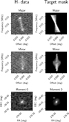 |
Fig. 3 Comparison between data from the H I cube (upper row) and the corresponding target mask (lower row) for a strong source in the development cube. The left column plot shows the intersection along the major axis and the middle column plot shows the minor axis. Gray pixels in the target occur due to rounding when computing slicing the cubic data. The right column plots show an equivalent to Moment 1 plots, that is, all voxel values summed over the frequency range corresponding to the vertical axis in left-hand side plots. |
2.3 Step II: Source characterization
With a trained segmentation CNN, the mask was retrieved by propagating an input H I cube into the model and binarizing the output with a threshold value. From here, we could utilize many of the modules in SOFIA 1.3.2 (Serra et al. 2015) to both extract contiguous segments and compute the corresponding attributes. First, the binary mask was passed as input to the merging module, which efficiently merges disconnected segments regarded as being close enough and rejects segments being too small. From the output list of this module estimates of the source centroid sky coordinates (α°, δ°), the central frequency, vcentral, and the line width, w20, were provided.
For the remaining attributes, we found that for faint sources the routines implemented in SOFIA were not suitable for the masks given by the segmentation CNN. Therefore, we implemented these computations ourselves. To compute the major and minor axis, the obtained 3D mask was projected onto the x, y-plane to get a structure similar to the galaxy ellipse. The sizes of the axes were then determined by taking the two principal components from the set of 2D positions of the projected mask. From the estimation of the two axes, the inclination was calculated by the relationship between the axes ratio in Eq. (1). Similarly, the position angle, θ, was computed by principal component analysis, but performed on the 3D mask instead. Since the position angle, θ, was defined as the angle of the major axis of the receding side of the galaxy, the angle of the first principal component, projected onto the x, y-plane, was used. In order to distinguish which end of the major axis corresponds to the receding side, the sign of this principal component over the frequency axis was used.
To compute the line flux integral, F, we utilized the dilation module in SOFIA, which increments the mask size until a maximum integrated flux is reached. From such a dilated mask, the line flux integral, F, was computed by summing up voxel values corresponding to all voxels marked in the dilated mask.
By thresholding the CNN output, and as provided by SOFIA, there were additional parameters to set in this step: the mask threshold, minimum line flux integral, maximum line flux integral, minimum radius for separated sources to be merged, minimum and maximum size in each direction of the cube, and the minimum number of voxels of the source, and maximum mask dilation. All of these had an impact on the generated source catalog. In the case of SDC2, the goal was to obtain the maximum score according to a pre-defined scoring function. We employed an algorithm for hyperparameter optimization, Tree of Parzen Estimator (TPE; Bergstra et al. 2011), with the same objective as the scoring function in the challenge, to find appropriate parameter values. In the general use case of our source detection pipeline, this scoring function may not be an appropriate metric and is instead up to the user to define. In this paper, we do not consider a single objective function to be optimized, however, we analyze in Sect. 3 how the parameter values affected the pipeline performance.
 |
Fig. 4 Flowchart of the sampling procedure for training and validation data. The left part, with blue arrows, illustrates sampled data set stored in memory: C galaxy container cubes and 4 C background training cubes. The right part, with orange arrows, illustrates sampling performed during training, resulting in p · 128 galaxy training cubes and (1 − p) · 128 background training cubes. |
2.4 Memory management for pipeline deployment
We developed and used the pipeline on two different types of machines: one at the Swiss National Supercomputing Centre (CSCS) Lugano, Switzerland, equipped with 64GB RAM and an NVIDIA Tesla P100 16GB, and one at Fraunhofer-Chalmers Centre equipped with 64 GB RAM and an NVIDIA GeForce GTX 1070 with 8GB GPU memory. To cope with these varying hardware constraints, we designed a method to apply the pipeline on an H I cube of any size, regardless of the memory constraints. To achieve this, the input H I cube was partitioned into sub-cubes, where each of the cubes was consecutively processed by the pipeline to produce one catalog for each sub-cube. The free memory needed for the pipeline scaled linearly to the size of the input cube and for that reason, the shapes of these sub-cubes were chosen to match hardware limitations. A final catalog for the full cube was finally produced by merging the catalogs.
To account for the risk of splitting a single source into two different sub-cubes, each sub-cube was expanded with padding. If a source was found with a center located in the padding region, it was rejected to be included in that sub-cube catalog. To still cover as much as possible of the whole cube, sub-cubes were arranged with overlap so that padding regions of one sub-cube were always included in the core region of another sub-cube. In our implementation, overlap regions were computed multiple times, so larger padding increased the execution time.
Similarly, we were flexible in choosing the input shape also for the segmentation CNN. Due to the convolutions and downsamplings in the model, the output voxel values of the segmentation CNN are determined by its neighborhood – the receptive field (Luo et al. 2016). Considering the receptive field centered at a voxel close to the boundary of an input cube, much of this region is missed in the input and therefore the output value of this voxel may be affected. To mitigate such potential damage, we added padding also to the CNN input cubes, but still arranged them so the effective output regions cover the full cube but padding on the very edge of the cube. Since regions inside the padding inevitably will be processed multiple times, larger padding will increase the computational cost. We did not investigate the actual receptive field for the trained CNN, but used the radius of the potential receptive field of the center voxel in the training cube, which was 16.
We had to consider two memory bottlenecks of the pipeline: processing the cube with the segmentation CNN constrained by the GPU memory and the SOFIA modules constrained by RAM. The execution time of the SOFIA modules scaled approximately linearly with the cube input size, but memory efficiency increased with the larger cube. With the padding fixed, determined by a minimum galaxy size to always be included, the most efficient arrangement strategy is to maximize the size of the mask passed to the SOFIA modules. Therefore, we let this define the size of the sub-cube and split it further into smaller cubes which were propagated through the segmentation CNN. The full arrangement, including the different padding regions, is visualized in Fig. 5.
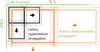 |
Fig. 5 Illustration of the arrangement of subsets of the full cube when applying the pipeline, projected into the two spatial dimensions. In the pipeline, this arrangement was also applied in the frequency dimension. Green lines denote the cube boundary, black and grey the regions processed in one batch of the galaxy segmentation step, and orange for one batch of the source characterization step. Dashed lines denotes padding in each of the steps. |
3 Analysis and results
In SDC2, the source-finding performance was measured by a scoring function computed from a cross-match between predicted and true source catalogs. For each entry in the predicted source catalog, the source’s score was set to −1 if the entry failed to be matched with a true source. If there was a match, the score was given by a value between 0 and 1, determined by the accuracy of the attribute estimates (see list of attributes in Table 1). The final score was computed by summing the source scores for all entries of the predicted source catalog. For comparison of our pipeline with other methods based on that metric, we recommend reviewing the results of the SDC2, as analyzed by (Hartley et al., in prep.). With the pre-defined penalty of −1 and de facto achievable estimation accuracy, this way of performance metric may implicitly favor a particular setting for reliability and completeness. In this section, we aim to analyze the performance of our pipeline in a much broader sense, by removing specific performance scoring on the individual attributes and focusing instead on exploring the parameter space of completeness and reliability. By adopting this approach, we can then explore the impact of performance on the estimated source attributes quantitatively and provide guidance for future applications in production.
In contrast to the SDC2 scoring, where the performance was calculated by only comparing the entries in the predicted source catalog and the true source catalog, we utilized the masks for a cross-matching purpose for the analysis in this section. Since these two ways of measuring the performance are fundamentally different, the results from the challenge are not comparable with the ones presented here. With access to the mask as predicted by the pipeline and true masks generated from the true source catalog using the procedure described in Sect. 2.2.2, we could use the intersection over union (IoU) metric (Minaee et al. 2021) to declare if a predicted source should be matched with a true source. This is a common performance metric for segmentation in computer vision and is defined as:
 (5)
(5)
for two sets A and B, which in our case were the voxels of a predicted and true mask. After employing the pipeline on the 40GB evaluation region from the challenge cube, visualized in Fig. 1, IoU was computed between each predicted source mask and all overlapping true masks. If the largest IoU among all those overlapping true masks for a predicted source was above 0.35, it was matched with the corresponding true source. Otherwise, when the predicted source could not be matched with any true source, it was regarded as a false positive.
For a predicted source catalog of P sources where M sources were matched, we defined reliability R as the number of matches divided by the number of detections:
 (6)
(6)
We note that the matching procedure could, in principle, allow for matching multiple predicted sources with the same true source. Therefore, the completeness, C, was defined as the number of matches divided by the number of true catalog sources:
 (7)
(7)
where D is the number of true sources matched with at least one predicted source and T is the length of the true source catalog. Our matching criterion turns out to be rather strict, meaning that the mask must recover a fairly large part of the galaxy. Therefore, the values of both reliability and completeness are lower than the corresponding values obtained with the SDC2 scoring.
As pointed out in Sect. 2.3, the parameter values of step II affected much of the characteristics of the predicted catalog. Therefore, employing the pipeline using a segmentation CNN trained on the development cube, the reliability and the completeness could be tweaked by the parameter values. In order to analyze the performance for different applications we used a fixed segmentation CNN, but sampled sets of parameter values in the space given by Table 2 to generate a variety of masks and catalogs. To perform such a sampling, we used the black box optimization algorithm TPE (Bergstra et al. 2011) to maximize the objective function:
![Mathematical equation: $ \alpha R + \left( {1 - \alpha } \right)C,\quad \alpha \in \left[ {0,\,1} \right], $](/articles/aa/full_html/2023/03/aa45139-22/aa45139-22-eq10.png) (8)
(8)
where a new value of α was randomly selected before each sampling. By varying α in this way, TPE was driven to sample parameter values preferred in different settings of importance for completeness C and reliability R, respectively.
Although the sampling procedure was designed to give parameter values preferable in different settings, many of the obtained parameter values were not desired in any setting at all. Therefore, after the set of parameter values were obtained through the sampling procedure, a “best ranking” metric was calculated to indicate which sets of parameter values that were preferred over other for any α. The calculation was performed by iteratively generating a sequence of the sets of parameter values sorted according to Eq. (8) for all α ∈ [0,1], which gave a unique sequence. Then, for each set of parameter values, the best ranking was determined as the lowest index it got among all the different sequences, corresponding to the different values of α. Hence, a small number of this metric means that the set of parameter values may be preferable in some setting, while a large number means it was not. The “best ranking” metric together with completeness, C, reliability, R, and source attribute estimation errors are visualized in Fig. 6.
Among the set of parameter values with low best ranking, there is a clear trade-off regarding the completeness and reliability. While the most reliable set of parameter values have reliability close to 1 and completeness around 0.02, the completeness is increased up to 0.07 at the cost of decreasing reliability down to 0.85. For each of the source attributes, there is an almost linear association between the reliability and the estimation error, so that they are negatively correlated. The dispersion in the reliability-error association is characterized differently for each attribute, where the position angle and the inclination are more distinct compared to the other. Most clearly for the line width, but also for the line flux integral, the spread of the estimation error is larger among the high-reliability sets of parameter values compared to the low-reliability sets. There are also outliers in the associations, but they are dominated by sets of parameter values that do not perform well for any value of α.
As shown in Fig. 6, completeness values of the sampled sets of parameter values do not go beyond 8% when measured against the full true catalog. This is expected as the flux distribution of sources, as bulk sources in the true catalog are weak (see Hartley et al., in prep.). To characterize the method it is important however to analyze the completeness with respect to the integrated line flux, which is shown in Fig. 7. From that perspective we see that completeness is, in general, higher for sources with a larger integrated line flux among all sets of parameter vales. However, high-completeness sets do not only detect more faint sources than high-reliability sets, but also more sources at the end tail of sources with the largest integrated line fluxes.
As it is shown in Figs. 6 and 7, the value of reliability does vary among the explored sets of parameters and its trade-off has an impact on the completeness of the predicted catalogs. Given this set of variously reliable sets, we can now reverse the question and investigate the maximum reliability that any given source in the true catalog can achieve through our pipeline. The maximum reliability of a particular source should correspond to the difficulty to distinguish it from false detection, which can be viewed as a proxy for the source’s detectability using our pipeline. In Fig. 8, we see that there is some degree of association between the maximum reliability and the line flux integral. For the very brightest sources, above 70 Jy Hz, the max reliability is almost the same for all of these source. Below that integrated flux level, there is some degree of linear association between line flux integral and the maximum reliability. The variance of this linear association is larger when the line flux integral is smaller, meaning that the prediction performance may decrease. A remark here is that the large number of undetected sources cannot be included in the scatter plot. Hence, the predictability of the maximal reliability may be less precise than the scatter plot alone would suggest.
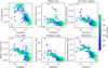 |
Fig. 6 Performance of the sampled sets of parameter values for step II. Each dot represent a single set of parameter values, as listed in Table 2, and its color is set by the best ranking (see text). The best forming set of parameter values, that have a small best ranking value, are colored green, while the worst with a large best ranking are colored in blue. The upper left plot shows completeness C as defined in Eq. (7) and reliability, R, as defined in Eq. (6), on the vertical and horizontal axis, respectively. In each of the other five plots, the attribute errors are plotted on the vertical axis, with reliability, R, on the horizontal axis. For major axis, line flux integral and line width, the value on the vertical axis is the median relative error. For the position angle and inclination, the value on the vertical axis is the median absolute error. For a predicted value of ŷ and a true value of y, the relative error is given by |ŷ – y|/y, while the absolute error is given by |ŷ – y|. |
Parameters of the source characterization step and their respective range used for sampling parameter values.
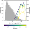 |
Fig. 7 Completeness in bins of integrated line flux of the sets of parameter with best ranking 1 in Fig. 6. Completeness for each line and level of integrated flux is shown on the right vertical axis, while the overall reliability of the set is given by the line color. The histogram in gray shows the distribution of all sources in the test set, with counts on the left vertical axis. We note that the scale on the horizontal axis is logarithmic. |
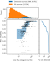 |
Fig. 8 Maximum catalog reliability among true sources detected by at least one predicted source catalog. Each dot represents a detected true source, located horizontally by its line flux integral and vertically by the maximum reliability. The blue background in the scatter plot shows the range between the 10th and the 90th percentile in maximum reliability of ten equally sized sets of detected sources, grouped by the line flux integral. The top histogram compares the integrated line flux distributions of all sources in the true source catalog with all detected sources. The right-hand side plot shows the cumulative fraction of detected sources, starting from the sources with highest max reliability. |
4 Discussion and future work
The results in Sect. 3, together with the results achieved in SDC2 (Hartely et al., in preparation), may suggest that our pipeline is useful when there exists a pre-defined source catalog on a portion of the data that can be utilized for supervised learning. Still, we see a number of challenges that should be addressed before setting our pipeline, or its descendants, into production. Most importantly, we argue that there is a need for a convenient performance metric aimed for unifying multiple purposes of a pipeline and that transfer between simulated and real data must be further studied. We believe many of the issues that we discuss in this section are not only specific to our pipeline, but could be addressed as needs emerge as machine learning approaches are being incorporated into the field of source finding.
4.1 Modifying pipeline components
Since the segmentation u-net used in our pipeline is aimed for a general purpose (e.g., medical imaging, see Sect. 2.2.1), there might be adaptations to the domain that could improve the performance. A reasonable example of how the model could be tweaked in this case is the size and shape of the filters in the convolution layers. Unlike the case of H I line data, in typical image applications of u-net, the axes have the same characteristics in every direction and a cubic shape is reasonable. Since the line width of a galaxy, measured in number of voxels in the data cube, is typically way larger than its disk diameter, a filter with a shape longer in the frequency dimension may be beneficial. Such a filter was implemented by the SDC2 winning team MINERVA (Hartley et al., in prep.).
Other potential improvements might be related to the construction of the segmentation target (Sect. 2.2.2), which was based on simplistic assumptions of the velocity profile that do not always hold. Most notably, the assumption that the largest orbital speed is obtained at the disk’s boundary is often violated. A simple adjustment to be applied to mitigate such a problem could be to allow for a bound of orbital speed also at this position – but to what extent is up for future work.
Another issue not taken into account by our target mask is the disk simplification, deviating from the ellipsoid assumption in the simulation. This is a simplification even compared to the simulation, where the shapes of the galaxies are modeled as ellipsoids. Considering ellipsoids instead of disks would not affect the upper bound in Eq. (2a), and the lower bound of the lower row, while the lower bound would be decreased.
4.2 Unifying performance metrics across applications
In Sect. 3, we used IoU of 0.35 between predicted masks and the ones constructed as in Sect. 2.2.2 to cross-match predicted and true sources. In Fig. 6, we can see that increased reliability from such a matching procedure gives in general better attribute estimates. This may indicate that a better overlap with our masks gives better source catalogs. However, this matching procedure is not sufficient for a universal comparison between any source finder. In fact, this cross-matching procedure, relying upon the same kind of masks as used in training and the chosen IoU threshold, is most likely only applicable in this work specifically. For the field in general, a convenient matching procedure should not involve masks at all since the essential problem is to generate the catalog, which can be solved with varying kinds of intermediate steps and not only binary masks. The matching used in SDC2 (Hartley et al., in prep.), based on only the properties of Table 1, could be an attractive procedure since it only requires a generated and a true source catalog.
In the related computer vision problems of object detection and instance segmentation, much of the machine learning progress in recent years can be attributed to the frequent benchmarking of different algorithms on a few but well-used data sets such as Pascal VOC (Everingham et al. 2009) and MS COCO (Lin et al. 2014). However, another important aspect that has allowed for the rapid development of the field is also the usage of general-purpose metrics, that take a range of applications into account. Even with a convenient matching procedure, there is still a tradeoff between reliability and completeness, as shown in Fig. 6, that is not reflected in the official SDC2 scoring mentioned above.
An intuitive way of achieving such general-purpose metric would be to give a score that is proportional to the difficulty in detecting the source, making strong sources more costly to miss. However, as shown in Figs. 7 and 8, predicting the detection difficulty for sources individually with our pipeline may be problematic. A common setup in the aforementioned machine learning benchmarks (but not in accordance with the one in SDC2) is that the algorithm must not only give the detected objects, but also a confidence score for each of them. Based on an algorithm that is able to accurately estimate confidence, the catalog can be filtered depending on reliability requirements. Hence, a single generated catalog can be utilized for multiple purposes, despite the presence of a tradeoff. The confidence score is utilized in performance metrics such as the average precision metric (Padilla et al. 2020), which is computed by the reliability multiplied by the completeness averaged for every possible confidence score-filtered catalog.
Estimating the confidence of each predicted source has been studied earlier in the field, for instance, by Serra et al. (2012). This algorithm was not employed in our pipeline, although it is implemented as a module in SOFIA. However, our results indicate that also the sets of step II parameter values might be used for such a purpose: by knowing the expected reliability of a set of parameter values, the reliability should be reflected by the maximum parameter set reliability similar to Fig. 8. By cross-matching different predicted catalogs produced by different sets of parameter values, the reliability of a single source may correspond to the highest expected reliability of the predicted catalogs in which it was included.
4.3 Apply pipeline to real data
An key limitation of this work is that we have only considered simulated data and we have not tried the pipeline on any real observation. The main worry when applying machine learning for a real problem when training has been performed on simulated data is that any bias in a simulation may be transferred and ultimately could degrade performance. For example, the simulated data may only cover a limited set of potential outcomes, meaning our pipeline was neither developed nor evaluated for features that were not included in the simulation. For the case of the SKA SDC2 data, there was a very low number of absorption feature occurrences in the data cubes. Therefore, we did not prioritize any special treatment of those sources when developing the pipeline since the few occurrences in the evaluation data probably had only a minor effect on the results. Moreover, the spiral galaxies simulated and ingested in the challenge data cube consisted of low-resolution versions of real H I observations of a small number of nearby galaxies. The pipeline has therefore not been trained to find signals that deviate from those spiral galaxies.
An interesting aspect to note is that the most data-hungry task, namely, training the segmentation CNN, is performed on data that is clearly biased with respect to the distribution of galaxies and background. Still, the source characterization is tunable to produce the reliability-completeness tradeoff. This suggests that at least some steps could possible be performed on somewhat biased simulated data, followed by tuning parameters in step II based on a smaller amount of real data.
5 Conclusions
We have developed a machine learning-driven pipeline for finding H I line sources that demonstrates reliable performance in predicting source catalogs from the simulated data in SDC2 (Hartley et al., in prep.). By only assuming simplistic properties of the spiral galaxies listed in the true source catalog, we generated a target mask that was suitable for training a segmentation CNN. In the final pipeline, the trained segmentation CNN produces a mask from a H I data cube, from which the existing SOFIA software is used to efficiently create the predicted catalog. Hence, we hereby show that modern machine learning tools can successfully be combined with astronomical guidance and established software routines.
In our results, we see that parameters of the second pipeline step, namely, to create the catalog from the mask, can be varied to generate substantially different catalogs. Different parameter values may be favorable in different applications, in terms of a tradeoff between completeness and reliability. This suggests that the time-consuming task of training the segmentation CNN does not have to be performed for any new type of source finding purpose. However, to allow for such development, there is a need for general purpose metrics that measures performance for a range of settings of the reliability rather than a single one.
Acknowledgements
This work was supported by a grant from the Swiss National Supercomputing Centre (CSCS) under project ID sm47. We acknowledge support from the Onsala Space Observatory national infrastructure for the provisioning of its facilities/observational support. Onsala Space Observatory receives funding through the Swedish Research Council via grant no. 2017 – 00648. We also acknowledge support from the Fraunhofer Cluster of Excellence Cognitive Internet Technologies.
Appendix A Derivation of target mask
To derive the mask shape from the assumptions, we considered a disk-shaped galaxy with diameter S and infinitesimal thickness in ℝ3, tilted with an inclination, i, around the x-axis in a clockwise direction and with the position angle, θ, around the z-axis in an anti-clockwise direction. In a H I cube the center of the galaxy will be found at (x0, y0, vcentral), where the central frequency, vcentral, corresponds to the line-of-sight velocity vC. We parameterize the positions on the disk by the distance to the galaxy center, r ∈ [0,1], and the angle relative to the position angle, u ∈ [0, 2π). For example, points at the line u = 0 correspond to those along the major axis in the receding direction. The rotational speed of the disk at radius, r, is given by the function:
![Mathematical equation: $ {\upsilon _R}\left( r \right):\left[ {0,\,1} \right] \mapsto , $](/articles/aa/full_html/2023/03/aa45139-22/aa45139-22-eq11.png) (A.1)
(A.1)
so that the line-of-sight velocity is
 (A.2)
(A.2)
The source catalog tells us that
 (A.3)
(A.3)
and since we assume vR(r) to be the same for every direction u due to Eq. (A.2), it follows that
 (A.4)
(A.4)
Putting Eqs. (A.3) and (A.4) together gives
 (A.5)
(A.5)
With an orbital period T(r) for the circle with radius r, which is:

we assume due that the orbital period for any r satisfies:

or equivalently

Assuming that the rotational speed at the disk’s boundary is the maximum speed, that is,  , together with Eq. (A.5), then gives us:
 (A.6)
(A.6)
These inequalities include various possible line widths that fit inside a triangular shape, as illustrated in Fig. A.1. Our hope was that the true vR(r) should be in the set of valid functions, although we noted that velocity profile sometimes tends to be below the blue line in Fig. A.1. However, we concluded that this region captures the most salient features of the profile in most cases by visual inspection, as exemplified in Fig. 3.
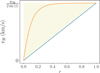 |
Fig. A.1 Velocity profiles covered by the mask (yellow shaded area), accompanied by two examples of velocity profiles (orange and blue lines). The two examples are a subset of all the velocity profiles that fit inside the yellow shaded area and thereby are represented by the mask. The horizontal axis shows the distance to the galaxy center r and the vertical axis displays the orbital speed vR. We note that r is a normalized value between 0 and 1, where 0 is the galaxy center and 1 is the edge. |
Expressing Eq. (A.6) as the line-of-sight velocities vz gives
 (A.7)
(A.7)
where  . This describes the occupied voxels of the mask. When constructing the mask, we defined the ellipse shape by using the major axis, S, inclination, i, and position angle, θ, from the source catalog. The minor axis, s, was computed by Eq. (1). For each pixel x, y, relative to the center and with a major axis along the x-axis, inside the ellipse we retrieved boundaries in the line-of-sight velocity by using

and

Appendix B Padding of the target mask
In this section, we give detailed formulation on how we constructed a modified version of Eq. (A.7) to account for padding to the target mask. Due to blur and noise in the data, not even a perfect galaxy model would be expected to eliminate the actual discrepancy between the mask and the galaxy voxels. It is for that reason that padding is included. For a padding of p ∈ ℝ0+, and pixels x, y (relative to the ellipse center), we define

and

From this, we define the following variables:

To improve readability we also define the function

The lower bounds of the occupied line-of-sight velocities are
 (B.1)
(B.1)
The upper bounds of the occupied line-of-sight velocities are
 (B.2)
(B.2)
In Figs. B.2 and B.1, the added padding is visualized as an illustration.
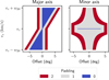 |
Fig. B.1 Illustrations of mask occupation for an example galaxy visualized as PV-diagrams, with positional offset from the galaxy center on the horizontal axis and line-of-sight velocity on the vertical axis. The cross-section along the major axis is shown in the left plot and along the minor axis in the right plot. The example galaxy has a major axis S = 10 and inclination i = 45°. The color denotes the occupation for three different levels of padding, including zero padding. |
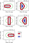 |
Fig. B.2 Other illustrations of mask occupation for the same example galaxy as in Fig. B.1, viewed by the cross-sections of different line-of-sight velocities. The green ellipse represents the shape given by the major and minor axis. The color denotes the occupation for three different levels of padding, including zero padding. |
Appendix C Training curve
In this section we give the progress of training and validation loss of the segmentation CNN, which can be seen in Fig. C.1, for reproducibility purposes.
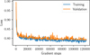 |
Fig. C.1 Progress of training and validation loss of the segmentation CNN. |
References
- Bergstra, J., Bardenet, R., Bengio, Y., & Kégl, B. 2011, Advances in Neural Information Processing Systems, 24 [Google Scholar]
- Bertels, J., Eelbode, T., Berman, M., et al. 2019, Lecture Notes in Computer Science, 11765, 92 [Google Scholar]
- Bonaldi, A., An, T., Brüggen, M., et al. 2021, MNRAS, 500, 3821 [Google Scholar]
- Braun, R., Bourke, T., Green, J. A., Keane, E., & Wagg, J. 2015, in Advancing Astrophysics with the Square Kilometre Array (AASKA14), 174 [Google Scholar]
- Çiçek, Ö., Abdulkadir, A., Lienkamp, S. S., Brox, T., & Ronneberger, O. 2016, Lecture Notes in Computer Science, 9901, 424 [CrossRef] [Google Scholar]
- De Blok, W. J., Walter, F., Brinks, E., et al. 2008, AJ, 136, 2648 [NASA ADS] [CrossRef] [Google Scholar]
- Everingham, M., Van Gool, L., Williams, C. K., Winn, J., & Zisserman, A. 2009, Int. J. Comput. Vis., 88, 303 [Google Scholar]
- Giovanelli, R., & Haynes, M. P. 2015, A&ARv, 24, 1 [Google Scholar]
- Glorot, X., Bordes, A., & Bengio, Y. 2011, Proceedings of Machine Learning Research, 15, 315 [Google Scholar]
- González, R. E., Muñoz, R. P., & Hernández, C. A. 2018, Astron. Comput., 25, 103 [CrossRef] [Google Scholar]
- He, K., Zhang, X., Ren, S., & Sun, J. 2016, Deep Residual Learning for Image Recognition [Google Scholar]
- Ioffe, S., & Szegedy, C. 2015, Proceedings of Machine Learning Research, 37, 448 [Google Scholar]
- Isensee, F., Kickingereder, P., Wick, W., Bendszus, M., & Maier-Hein, K. H. 2018, Lecture Notes in Computer Science, 11384, 234 [Google Scholar]
- Jadon, S. 2020, 2020 IEEE Conference on Computational Intelligence in Bioinformatics and Computational Biology, CIBCB 2020 [Google Scholar]
- Kingma, D. P., & Ba, J. 2014, 3rd International Conference on Learning Representations, ICLR 2015 – Conference Track Proceedings [Google Scholar]
- LeCun, Y., Bengio, Y., & Hinton, G. 2015, Nature 521, 436 [Google Scholar]
- Lin, T. Y., Maire, M., Belongie, S., et al. 2014, Lecture Notes in Computer Science, 8693, 740 [CrossRef] [Google Scholar]
- Liu, X., Deng, Z., & Yang, Y. 2018, Artif. Intell. Rev., 52, 1089 [Google Scholar]
- Lukic, V., Brüggen, M., Banfield, J. K., et al. 2018, MNRAS, 476, 246 [NASA ADS] [CrossRef] [Google Scholar]
- Lukic, V., Gasperin, F. D., & Brüggen, M. 2019, Galaxies, 8, 3 [NASA ADS] [CrossRef] [Google Scholar]
- Luo, W., Li, Y., Urtasun, R., & Zemel, R. 2016, Adv. Neural Inform. Process. Syst., 29 [Google Scholar]
- Masters, K. L., & Galaxy Zoo Team 2020, in Galactic Dynamics in the Era of Large Surveys, 353, eds. M. Valluri, & J. A. Sellwood, 205 [NASA ADS] [Google Scholar]
- Milletari, F., Navab, N., & Ahmadi, S. A. 2016, Proceedings – 2016 4th International Conference on 3D Vision, 3DV 2016, 565 [Google Scholar]
- Minaee, S., Boykov, Y. Y., Porikli, F., et al. 2021, IEEE Trans. Pattern Analy. Mach. Intell., 44, 3523 [Google Scholar]
- Nelson, S. 2008, Nature, 455, 36 [NASA ADS] [CrossRef] [Google Scholar]
- Nordström, M., Bao, H., Löfman, F., et al. 2020, Lecture Notes in Computer Science, 12264, 269 [CrossRef] [Google Scholar]
- Padilla, R., Netto, S. L., & Da Silva, E. A. 2020, International Conference on Systems, Signals, and Image Processing, 2020 July, 237 [Google Scholar]
- Ronneberger, O., Fischer, P., & Brox, T. 2015, Lecture Notes in Computer Science, 9351, 234 [CrossRef] [Google Scholar]
- Serra, P., Jurek, R., & Fler, L. 2012, PASA, 29, 296 [NASA ADS] [CrossRef] [Google Scholar]
- Serra, P., Westmeier, T., Giese, N., et al. 2015, MNRAS, 448, 1922 [Google Scholar]
- Taghanaki, S. A., Zheng, Y., Kevin Zhou, S., et al. 2019, Comput. Med. Imaging Graph., 75, 24 [CrossRef] [Google Scholar]
- Thoma, M. 2016, ArXiv e-prints [arXiv:1602.06541] [Google Scholar]
- Tian, C., Fei, L., Zheng, W., et al. 2020, Neural Netwo., 131, 251 [CrossRef] [Google Scholar]
- van de Hulst, H. C. 1945, Nederlandsch Tijdschrift voor Natuurkunde, 11, 210 [Google Scholar]
- Westmeier, T., Kitaeff, S., Pallot, D., et al. 2021, MNRAS, 506, 3962 [NASA ADS] [CrossRef] [Google Scholar]
- Whiting, M. T. 2012, MNRAS, 421, 3242 [NASA ADS] [CrossRef] [Google Scholar]
- Whiting, M., & Humphreys, B. 2012, PASA, 29, 371 [NASA ADS] [CrossRef] [Google Scholar]
- Yakubovskiy, P. 2020, Segmentation Models Pytorch, https://github.com/qubvel/segmentation_models.pytorch [Google Scholar]
A full description of the data and the challenge was provided in the file SCIENCE DATA CHALLENGE 2: DATA DESCRIPTION, published under the SDC2 website https://sdc2.astronomers.skatelescope.org/sdc2-challenge/description on February 1, 2021.
All Tables
Parameters of the source characterization step and their respective range used for sampling parameter values.
All Figures
|
Fig. 1 Flowchart for data usage. Generating a mask from a true source catalog refers to the procedure presented in Sect. 2.2.2 and training step is described in Sect. 2.2.3. Pipeline employment covers both steps of galaxy segmentation (Sect. 2.2) and source characterization (Sect. 2.3). The evaluation refers to the analysis performed in Sect. 3. |
| In the text | |
|
Fig. 2 Overview of the used u-net segmentation model for an example input cube of size 32 × 32 × 32. The encoder is formed by all grey vertical arrows pointing downwards on the plot, while the decoder consists of the remaining arrows on the right of the plot. The dashed lines separate the different resolutions, meaning that down- or upsampling actions are used to go between these. Black rectangles with numbers indicate the number of filters of the different stages. Gray arrows represent one or multiple ResNet blocks, each with one downsampling layer. Orange arrows represent upsampling layers, green represents copy and merger actions, and blue arrows represent a sequence of two decoder blocks. |
| In the text | |
|
Fig. 3 Comparison between data from the H I cube (upper row) and the corresponding target mask (lower row) for a strong source in the development cube. The left column plot shows the intersection along the major axis and the middle column plot shows the minor axis. Gray pixels in the target occur due to rounding when computing slicing the cubic data. The right column plots show an equivalent to Moment 1 plots, that is, all voxel values summed over the frequency range corresponding to the vertical axis in left-hand side plots. |
| In the text | |
|
Fig. 4 Flowchart of the sampling procedure for training and validation data. The left part, with blue arrows, illustrates sampled data set stored in memory: C galaxy container cubes and 4 C background training cubes. The right part, with orange arrows, illustrates sampling performed during training, resulting in p · 128 galaxy training cubes and (1 − p) · 128 background training cubes. |
| In the text | |
|
Fig. 5 Illustration of the arrangement of subsets of the full cube when applying the pipeline, projected into the two spatial dimensions. In the pipeline, this arrangement was also applied in the frequency dimension. Green lines denote the cube boundary, black and grey the regions processed in one batch of the galaxy segmentation step, and orange for one batch of the source characterization step. Dashed lines denotes padding in each of the steps. |
| In the text | |
|
Fig. 6 Performance of the sampled sets of parameter values for step II. Each dot represent a single set of parameter values, as listed in Table 2, and its color is set by the best ranking (see text). The best forming set of parameter values, that have a small best ranking value, are colored green, while the worst with a large best ranking are colored in blue. The upper left plot shows completeness C as defined in Eq. (7) and reliability, R, as defined in Eq. (6), on the vertical and horizontal axis, respectively. In each of the other five plots, the attribute errors are plotted on the vertical axis, with reliability, R, on the horizontal axis. For major axis, line flux integral and line width, the value on the vertical axis is the median relative error. For the position angle and inclination, the value on the vertical axis is the median absolute error. For a predicted value of ŷ and a true value of y, the relative error is given by |ŷ – y|/y, while the absolute error is given by |ŷ – y|. |
| In the text | |
|
Fig. 7 Completeness in bins of integrated line flux of the sets of parameter with best ranking 1 in Fig. 6. Completeness for each line and level of integrated flux is shown on the right vertical axis, while the overall reliability of the set is given by the line color. The histogram in gray shows the distribution of all sources in the test set, with counts on the left vertical axis. We note that the scale on the horizontal axis is logarithmic. |
| In the text | |
|
Fig. 8 Maximum catalog reliability among true sources detected by at least one predicted source catalog. Each dot represents a detected true source, located horizontally by its line flux integral and vertically by the maximum reliability. The blue background in the scatter plot shows the range between the 10th and the 90th percentile in maximum reliability of ten equally sized sets of detected sources, grouped by the line flux integral. The top histogram compares the integrated line flux distributions of all sources in the true source catalog with all detected sources. The right-hand side plot shows the cumulative fraction of detected sources, starting from the sources with highest max reliability. |
| In the text | |
|
Fig. A.1 Velocity profiles covered by the mask (yellow shaded area), accompanied by two examples of velocity profiles (orange and blue lines). The two examples are a subset of all the velocity profiles that fit inside the yellow shaded area and thereby are represented by the mask. The horizontal axis shows the distance to the galaxy center r and the vertical axis displays the orbital speed vR. We note that r is a normalized value between 0 and 1, where 0 is the galaxy center and 1 is the edge. |
| In the text | |
|
Fig. B.1 Illustrations of mask occupation for an example galaxy visualized as PV-diagrams, with positional offset from the galaxy center on the horizontal axis and line-of-sight velocity on the vertical axis. The cross-section along the major axis is shown in the left plot and along the minor axis in the right plot. The example galaxy has a major axis S = 10 and inclination i = 45°. The color denotes the occupation for three different levels of padding, including zero padding. |
| In the text | |
|
Fig. B.2 Other illustrations of mask occupation for the same example galaxy as in Fig. B.1, viewed by the cross-sections of different line-of-sight velocities. The green ellipse represents the shape given by the major and minor axis. The color denotes the occupation for three different levels of padding, including zero padding. |
| In the text | |
|
Fig. C.1 Progress of training and validation loss of the segmentation CNN. |
| In the text | |
Current usage metrics show cumulative count of Article Views (full-text article views including HTML views, PDF and ePub downloads, according to the available data) and Abstracts Views on Vision4Press platform.
Data correspond to usage on the plateform after 2015. The current usage metrics is available 48-96 hours after online publication and is updated daily on week days.
Initial download of the metrics may take a while.