| Issue |
A&A
Volume 675, July 2023
BeyondPlanck: end-to-end Bayesian analysis of Planck LFI
|
|
|---|---|---|
| Article Number | A6 | |
| Number of page(s) | 26 | |
| Section | Cosmology (including clusters of galaxies) | |
| DOI | https://doi.org/10.1051/0004-6361/202243619 | |
| Published online | 28 June 2023 | |
BEYONDPLANCK
VI. Noise characterization and modeling
1
Institute of Theoretical Astrophysics, University of Oslo, Blindern, Oslo, Norway
e-mail: This email address is being protected from spambots. You need JavaScript enabled to view it.
2
Dipartimento di Fisica, Università degli Studi di Milano, Via Celoria 16, Milano, Italy
3
INAF-IASF Milano, Via E. Bassini 15, Milano, Italy
4
INFN, Sezione di Milano, Via Celoria 16, Milano, Italy
5
INAF – Osservatorio Astronomico di Trieste, Via G.B. Tiepolo 11, Trieste, Italy
6
Planetek Hellas, Leoforos Kifisias 44, Marousi, 151 25
Greece
7
Department of Astrophysical Sciences, Princeton University, Princeton, NJ, 08544
USA
8
Jet Propulsion Laboratory, California Institute of Technology, 4800 Oak Grove Drive, Pasadena, California, USA
9
Department of Physics, Gustaf Hällströmin katu 2, University of Helsinki, Helsinki, Finland
10
Helsinki Institute of Physics, Gustaf Hällströmin katu 2, University of Helsinki, Helsinki, Finland
11
Computational Cosmology Center, Lawrence Berkeley National Laboratory, Berkeley, California, USA
12
Haverford College Astronomy Department, 370 Lancaster Avenue, Haverford, Pennsylvania, USA
13
Max-Planck-Institut für Astrophysik, Karl-Schwarzschild-Str. 1, 85741 Garching, Germany
14
Dipartimento di Fisica, Università degli Studi di Trieste, Via A. Valerio 2, Trieste, Italy
Received:
23
March
2022
Accepted:
17
June
2022
Abstract
We present a Bayesian method for estimating instrumental noise parameters and propagating noise uncertainties within the global BEYONDPLANCK Gibbs sampling framework, which we applied to Planck Low Frequency Instrument (LFI) time-ordered data. Following previous works in the literature, we initially adopted a 1/f model for the noise power spectral density (PSD), but we found the need for an additional lognormal component in the noise model in the 30 and 44 GHz bands. We implemented an optimal Wiener-filter (or constrained realization) gap-filling procedure to account for masked data. We then used this procedure to both estimate the gapless correlated noise in the time-domain, ncorr, and to sample the noise PSD parameters, ξn = {σ0, fknee, α, Ap}. In contrast to previous Planck analyses, we assumed piecewise stationary noise only within each pointing period (PID), and not throughout the full mission, but we adopted the LFI Data Processing Center results as priors on α and fknee. We generally found best-fit correlated noise parameters that are mostly consistent with previous results, with a few notable exceptions. However, a detailed inspection of the time-dependent results has revealed many important findings. First and foremost, we find strong evidence for statistically significant temporal variations in all noise PSD parameters, many of which are directly correlated with satellite housekeeping data. Second, while the simple 1/f model appears to be an excellent fit for the LFI 70 GHz channel, there is evidence for additional correlated noise that is not described by a 1/f model in the 30 and 44 GHz channels, including within the primary science frequency range of 0.1–1 Hz. In general, most 30 and 44 GHz channels exhibit deviations from 1/f at the 2–3σ level in each one-hour pointing period, motivating the addition of the lognormal noise component for these bands. For certain periods of time, we also find evidence of strong common mode noise fluctuations across the entire focal plane. Overall, we conclude that a simple 1/f profile is not adequate for obtaining a full characterization of the Planck LFI noise, even when fitted hour-by-hour, and a more general model is required. These findings have important implications for large-scale CMB polarization reconstruction with the Planck LFI data and the current work is a first attempt at understanding and mitigating these issues.
Key words: cosmology: observations / cosmic background radiation / diffuse radiation / polarization / methods: data analysis
© The Authors 2023
 Open Access article, published by EDP Sciences, under the terms of the Creative Commons Attribution License (https://creativecommons.org/licenses/by/4.0), which permits unrestricted use, distribution, and reproduction in any medium, provided the original work is properly cited.
This article is published in open access under the Subscribe to Open model. This email address is being protected from spambots. You need JavaScript enabled to view it. to support open access publication.
1. Introduction
One of the main algorithmic achievements made within the field of cosmic microwave background (CMB) analysis over the past few decades is a method of data compression that is both accurate and nearly lossless. Starting from data sets that typically comprise 𝒪(108 − 1011) time-ordered measurements, we are now able to routinely produce sky maps that contain 𝒪(103 − 107) pixels (e.g., Tegmark 1997; Ashdown et al. 2007). From these, we may constrain the angular CMB power spectrum, which spans 𝒪(103) multipoles (e.g., Gorski 1994; Hivon et al. 2002; Wandelt et al. 2004). Finally, we may use this data to derive tight constraints on a small set of cosmological parameters (e.g., Bond et al. 2000; Lewis & Bridle 2002; Planck Collaboration V 2020; Planck Collaboration VI 2020), which is typically the ultimate goal of any CMB experiment.
Two fundamental assumptions underlying this radical compression process are: the instrumental noise may be modeled to a sufficient precision and the corresponding induced uncertainties may be propagated faithfully to higher order data products. The usual starting point for this process is to assume that the noise is Gaussian and random in time and is not correlated with the true sky signal at any given time. Under the Gaussian hypothesis, the net noise contribution therefore decreases as  , where Nobs is the number of observations of the given sky pixel, while the signal contribution is independent of Nobs.
However, it is not sufficient to assume that the noise is simply Gaussian and random. We must also assume something about its statistical properties, both in terms of its correlation structure in time and its stationarity period. Regarding the correlation structure, the single most common assumption in the CMB literature is that the temporal noise power spectrum density (PSD) can be modeled as a sum of a so-called 1/f term and a white noise term (e.g., Bennett et al. 2013; Planck Collaboration II 2020; Planck Collaboration III 2020). The white noise term arises from intrinsic detector and amplifiers’ thermal noise and it is substantially reduced by cooling the instrument to cryogenic temperatures, typically to ∼20 K for coherent receivers, as in the case of Planck Low Frequency Instrument (LFI), and to 0.1–0.3 K for bolometric detectors. Traditionally, the white noise of coherent radiometers is expressed in terms of system noise temperature, Tsys, per unit integration time (measured in K Hz−1/2); whereas for bolometers, it is expressed as noise equivalent power, NEP (W Hz−1/2). The sources of the 1/f noise component include intrinsic instabilities in the detectors, amplifiers, and readout electronics, as well as environmental effects, and, notably, atmospheric fluctuations for sub-orbital experiments. In the case of Planck LFI, the 1/f noise was dominated by gain and noise temperature fluctuations and thermal instabilities (Planck Collaboration II 2020), and it was minimized by introducing the 4 K reference loads and gain modulation factor to optimize the receiver balance. We refer to Planck Collaboration II (2014, 2016) and BeyondPlanck Collaboration (2023) for further details.
Regarding stationarity, the two most common assumptions are either that the statistical properties remain constant throughout the entire observation period (e.g., Planck Collaboration II 2020), or that it may at least be modeled as piecewise stationary within, for instance, one hour of observations (e.g., QUIET Collaboration 2011). Given such basic assumptions, the effect of the instrumental noise on higher-order data products has then traditionally been assessed, and propagated, either through the use of detailed end-to-end simulations (e.g., Planck Collaboration XII 2016) or in the form of explicit noise covariance matrices (e.g., Tegmark et al. 1997; Page et al. 2007; Planck Collaboration V 2020).
The importance of accurate noise modeling is intimately tied to the overall signal-to-noise ratio (S/N) of the science target in question. For applications with very S/N, detailed noise modeling is essentially irrelevant, since other sources of systematic errors dominate the total error budget. One prominent example of this is the CMB temperature power spectrum as measured by Planck on large angular scales (Planck Collaboration IV 2020; Planck Collaboration V 2020). The white noise contribution to the power spectrum can be misestimated by several orders of magnitude without making any difference in terms of cosmological parameters. This is because the full error budget is vastly dominated by cosmic variance.
The cases for which accurate noise modeling is critically important feature S/N values on the order of unity. For these, noise misestimation may be the difference between obtaining a tantalizing, but ultimately unsatisfying, 2 σ result and claiming a ground-breaking and decisive 5 σ discovery – or, in the worst-case scenario, erroneously reporting a baseless positive detection.
This regime is precisely where the CMB field is expected to find itself in only a few years from now, as the next-generation CMB experiments (e.g., CMB-S4, LiteBIRD, PICO, Simons Observatory, and many others; Abazajian et al. 2019; Suzuki et al. 2018; Sugai et al. 2020; LiteBIRD Collaboration 2023; Hanany et al. 2019; Ade et al. 2019) are currently being planned, built, and commissioned in the context of the search for primordial gravitational waves imprinted in B-mode polarization. The predicted magnitude of this signal is expected to be at most a few tens of nanokelvins on angular scales larger than a degree, corresponding to a relative precision of 𝒪(10−8), and extreme precision is required for a robust detection. It has therefore become critically important to take into account all sources of systematic uncertainties, including correlated noise, and propagate these into the final results.
The BEYONDPLANCK project (BeyondPlanck Collaboration 2023) is an initiative that aims to meet this challenge by implementing the first global Bayesian CMB analysis pipeline that supports faithful end-to-end error propagation from raw time-ordered data to final cosmological parameters. One fundamental aspect of this approach is a fully parametric data model that is fitted to the raw measurements through standard posterior sampling techniques, simultaneously constraining both instrumental and astrophysical parameters. Within this framework, the instrumental noise is just one among many different sources of uncertainty, all of which are treated on the same statistical basis. The sample-based approach introduced by BEYONDPLANCK therefore represents a third and novel way of propagating noise uncertainties (Keihänen et al. 2023; Suur-Uski et al., in prep.), complementary to the existing simulation and covariance matrix based approaches used by traditional pipelines.
As a real-world demonstration of this novel framework, the BEYONDPLANCK collaboration has chosen the Planck LFI measurements (Planck Collaboration I 2020; Planck Collaboration II 2020) as its main scientific target (BeyondPlanck Collaboration 2023). These data represent an important and realistic testbed in terms of overall data volume and complexity, and they also offer fairly well-understood properties after more than a decade of detailed scrutiny by the Planck team (see Planck Collaboration II 2014, 2016, 2020, and references therein). However, as reported in this paper, there are still a number of subtle unresolved and unexplored issues relating to this important and well-studied data set that potentially may have an impact on higher-level science results. Furthermore, as demonstrated by the current analysis, the detailed low-level Bayesian modeling approach is ideally suited to identify, study, and eventually mitigate these effects.
Thus, the present paper has two main goals. The first is to describe the general algorithmic framework implemented in the BEYONDPLANCK pipeline for modeling instrumental noise in CMB experiments. The second goal is then to apply these methods to the Planck LFI observations and characterize the performance and systematic effects of the instrument as a function of time and the detector.
The rest of the paper is organized as follows. First, in Sect. 2, we briefly review the BEYONDPLANCK analysis framework and data model, with a particular emphasis on the noise modeling aspects. In Sect. 3, we present the individual sampling steps required for noise modeling, as well as some statistics that are useful for efficient data monitoring. In Sect. 4, we discuss various important degeneracies that are relevant for noise modeling and ways of minimizing the impact of modeling errors. Next, in Sect. 5, we give a high-level overview of the various noise posterior distributions and their correlation properties, as well as detailed specifications for each detector. In Sect. 6, we discuss anomalies found in the data and interpret these in terms of the instrument and the thermal environment. Finally, we summarize our conclusions in Sect. 7.
2. BEYONDPLANCK data model and framework
The BEYONDPLANCK project is an attempt to build up an end-to-end data analysis pipeline for CMB experiments going all the way from raw time-ordered data to cosmological parameters in a consistent Bayesian framework. This allows us to characterize degeneracies between instrumental and astrophysical parameters in a statistically well-defined framework, from low-level instrumental quantities such as gain (Gjerløw et al. 2023), bandpasses (Svalheim et al. 2023a), far sidelobes (Galloway et al. 2023a), and correlated noise via Galactic parameters that include the synchrotron amplitude or spectral index (Andersen et al. 2023; Svalheim et al. 2023b), and up to the angular CMB power spectrum and cosmological parameters (Colombo et al. 2023; Paradiso et al. 2023).
The LFI dataset consists of three bands, at frequencies of roughly 30, 44, and 70 GHz. These bands have two, three, and six radiometer pairs each, respectively, which (for historical reasons) are numbered from 18 to 28. The two radiometers in each pair are labeled as M and S1 (Planck Collaboration II 2014). In BEYONDPLANCK, the raw uncalibrated data, d, produced by each of these radiometers is modeled in the time domain as follows:
![Mathematical equation: $$ \begin{aligned}&d_{j,t} = g_{j,t} \mathtt{P}_{tp,j}\left[\mathtt{B}^{\mathrm{symm} }_{pp^{\prime },j}\sum _{c} \mathtt{M}_{cj}(\beta _{p^{\prime }}, \Delta _\mathrm{bp} ^{j})a^c_{p^{\prime }} + \mathtt{B}^{\mathrm{asymm} }_{pp^{\prime },j}\left(s^{\mathrm{orb} }_{j,t} + s^{\mathrm{fsl} }_{j,t}\right)\right] \nonumber \\&\qquad + s^{\mathrm{1hz} }_{j,t} + n^{\mathrm{corr} }_{j,t} + n^{\mathrm{wn} }_{j,t}. \end{aligned} $$](/articles/aa/full_html/2023/07/aa43619-22/aa43619-22-eq2.gif) (1)
(1)
Here the subscript t denotes a sample index in time domain; j denotes radiometer; p denotes the pixel number; c is an index denoting the different signal components; g denotes the gain; P denotes the pointing matrix; Bsymm and Basymm denote the symmetric and asymmetric beam matrices, respectively; a are the astrophysical signal amplitudes; β are the corresponding spectral parameters; Δbp are the bandpass corrections; Mcj is the bandpass-dependent component mixing matrix; sorb is the orbital dipole; sfsl are the far sidelobe corrections; s1hz represents electronic 1 Hz spike corrections; ncorr is the correlated noise; and nwn is the white noise. For more details on each of these parameters, we refer to BeyondPlanck Collaboration (2023) and its companion papers.
Let us denote the combined set of all free parameters by ω ≡ {g, ncorr, ξn, Δbp, ncorr, a, β, Cℓ}. Here, we have defined the noise power spectral density (PSD) parameters, ξn ≡ {σ0, fknee, α, Ap}. The goal of the Bayesian approach is now to sample from the joint posterior distribution,
 (2)
(2)
where the notation P(A ∣ B) indicates the conditional probability of A given B (i.e., keeping B fixed). This is a large and complicated distribution, with many degeneracies. However, using Gibbs sampling we can divide the sampling process into a set of managable steps. Gibbs sampling is a simple algorithm in which samples from a joint multi-dimensional distribution are generated by iterating through all corresponding conditional distributions. Using this method, the BEYONDPLANCK sampling scheme may be summarized as follows (BeyondPlanck Collaboration 2023),
 (3)
(3)
 (4)
(4)
 (5)
(5)
 (6)
(6)
 (7)
(7)
 (8)
(8)
 (9)
(9)
Here, ← indicates sampling from the distribution on the right-hand side.
We note that for some of these steps, we did not follow the strict Gibbs approach of conditioning on all but one variable. Most notably for us, this is the case for the gain sampling step in Eq. (3), where we did not set any condition on ncorr. In effect, we instead sampled the gain and correlated noise jointly by exploiting the definition of a conditional distribution:
 (10)
(10)
This equation implies that a joint sample {g, ncorr} may be produced by first sampling the gain from the marginal distribution with respect to ncorr, and then sampling ncorr from the usual conditional distribution with respect to g. The advantage of this joint sampling procedure is a much shorter Markov correlation length as compared to standard Gibbs sampling, as discussed by Gjerløw et al. (2023).
A convenient property of Gibbs sampling is its modular nature, as the various parameters are sampled independently within each conditional distribution, but the joint dependencies are still explored through the iterative scheme. In this paper, we are therefore only concerned with two of the above steps, namely Eqs. (4) and (5). For details on the complete Gibbs chain and the other sampling steps, we refer to BeyondPlanck Collaboration (2023) and its companion papers.
When sampling the correlated noise, we want to allow for the possibility that the noise properties change over time. Perhaps the simplest way to allow for this (thus, the approach we adopt in this paper) is to divide the data into chunks of time and assume that the noise properties are constant within each chunk and independent between chunks. The next step is then to choose the timescale, tchunk, over which we assume that the noise properties are stationary. There are a number of considerations that are relevant for deciding this timescale. In general, there are at least three important timescales to consider, namely the scanning period, tscan (i.e., how long it takes between the telescope comes back to roughly the same position on the sky, which is about 60 seconds for Planck), the correlated noise timescale tcorr ∼ 1/fknee (i.e., the timescale at which the correlated noise becomes relevant compared to the white noise, typically 10–100 s for LFI), and the timescale at which the noise properties change, tchange (which strongly depends on what gives rise to the change). Ideally we would want to chunk the data at a timescale that is much longer than the two former and much shorter than the latter timescale, that is, tscan, tcorr ≪ tchunk ≪ tchange. However, as changes to the noise properties can occur both suddenly due to glitches or sudden changes in the thermal environment (as is discussed in Sect. 6) or drift slowly over time, the last of the three timescales is not always well defined.
Another factor to consider is that if we are using Fourier transforms of the timestreams (or any other analysis that can be scaled superlinearly with the chunk size over time), a larger chunk size would be more computationally expensive. In general, the details of the specific data are very relevant, even if we do not have a completely well defined way to determine an optimal chunk size. The sample rate of the LFI time-ordered data is 32.5079 Hz, 46.5455 Hz, and 78.7692 Hz for the 30, 44, and 70 GHz bands, respectively.
The LFI time-ordered data are divided into roughly 45 000 pointing periods, denoted PIDs (pointing ID), during which the satellite spin axis direction remained fixed (see Planck Collaboration II 2011 for details on the Planck scanning strategy). Most PIDs have a duration of 30–60 min, which is at least an order of magnitude longer than both the scanning period and the correlated noise timescale for LFI, so they are a natural and convenient choice for chunking the data. Therefore, when sampling the correlated noise and the corresponding PSD parameters, we assume that the noise is stationary within each PID, but independent between PIDs. The gain is also assumed to be constant within each PID, however, this is not fit independently for each PID, but rather sampled smoothly on longer timescales (Gjerløw et al. 2023).
Following previous works in the literature (Mennella et al. 2010; Planck Collaboration II 2014, 2020), we start by assuming that the noise PSD may be described by a so-called 1/f model:
![Mathematical equation: $$ \begin{aligned} P(f) = \sigma _0^2\left[1 + \left(\frac{f}{f_\mathrm{knee} }\right)^\alpha \right]\!. \end{aligned} $$](/articles/aa/full_html/2023/07/aa43619-22/aa43619-22-eq12.gif) (11)
(11)
Here, f denotes a temporal frequency; σ0 quantifies the white noise level of the time-ordered data2; α is the slope (typically negative) of the correlated noise spectrum; and the knee frequency, fknee, denotes the (temporal) frequency at which the variance of the correlated noise is equal to the white noise variance.
While the 70 GHz noise properties are well described with the 1/f model, we show in the following that this model is not sufficient for representing the noise properties of the 30 and 44 GHz bands. These detectors often show a small amount of excess power at intermediate temporal frequencies (0.01–1 Hz), which is not adequately fit by the 1/f model. In order to address this, we allow for an additional lognormal component in the noise PSD for these bands:
![Mathematical equation: $$ \begin{aligned} P(f) = \sigma _0^2\left[1 + \left(\frac{f}{f_\mathrm{knee} }\right)^\alpha \right] + A_\mathrm{p} \exp \left[-\frac{1}{2}\left(\frac{\log _{10}f - \log _{10} f_\mathrm{p} }{\sigma _\mathrm{dex} }\right)^2\right]\!, \end{aligned} $$](/articles/aa/full_html/2023/07/aa43619-22/aa43619-22-eq13.gif) (12)
(12)
where Ap and fp are the amplitude and the frequency of the peak of the lognormal component, and σdex denotes the width of the component, in dex, around this peak. As the deviations from the 1/f model are small, and not very significant in a single PID, we are not be able to estimate the three parameters of the lognormal, Ap, fp, and σdex, for each PID. For this reason, we keep fp and σdex fixed, and only sample Ap for each PID.
We used a fairly wide lognormal centered on fp = 0.011 Hz with a width of σdex = 1 in order to accomodate excess power across a wide range of frequencies. A more detailed analysis would fit individual values for fp and σdex for each radiometer, allowing for an even better model fit; however, we find that the current model leads to acceptable model fits, as quantified in the time stream χ2 values, for all radiometers. The four PSD parameters that we go on to fit are then collectively denoted ξn = {σ0, fknee, α, Ap}.
The choice of using a lognormal component to parametrize the deviations from the 1/f model, as opposed to other ways of extending the noise model, is not motivated by any fundamental considerations. Rather, we simply want to add an extra degree of freedom to the noise model in the relevant frequency range and we found that a lognormal component was a practical way to do this. By using a lognormal, which decays both at high and low frequencies, we can use the high frequencies to determine the white noise level, σ0, and the low frequencies to measure fknee and α. In this way we reduce the degeneracy between the added noise component and the 1/f parameters, although some level of degeneracy between them is inevitable.
3. Methods
As outlined above, noise estimation in the Bayesian BEYONDPLANCK framework amounts to essentially being able to sample from two conditional distributions, namely, P(ncorr ∣ d, ω \ ncorr) and P(ξn ∣ d, ω \ ξn), where A \ B denotes all the elements of the set A except the ones also present in B. The first presentation of Bayesian noise estimation for time-ordered CMB data that was applicable to the current problem was presented by Wehus et al. (2012) and the main novel feature presented in the current paper is simply the integration of these methods into the larger end-to-end analysis framework outlined above. In addition, the current analysis also employs important numerical improvements as introduced by Keihänen et al. (2023), in which optimal mapmaking is re-phrased into an efficient Bayesian language.
The starting point for both conditional distributions is the following parametric data model,
 (13)
(13)
where d denotes the raw time ordered data (TOD) organized into a column vector; g is the gain;
![Mathematical equation: $$ \begin{aligned} \boldsymbol{s}^\mathrm{tot} \equiv \mathtt{P}\left[\mathtt{B}^{\mathrm{symm} } \mathtt{M}a + \mathtt{B}^{\mathrm{asymm} }\left(s^{\mathrm{orb} } + s^{\mathrm{fsl} }\right)\right]\!, \end{aligned} $$](/articles/aa/full_html/2023/07/aa43619-22/aa43619-22-eq15.gif) (14)
(14)
describing the total sky signal, comprising both CMB and foregrounds, projected into time-domain; s1hz represents electronic 1 Hz spike corrections; ncorr represents the correlated noise in the time domain; and nwn is white noise. The two noise terms are both assumed to be Gaussian-distributed with covariance matrices  and
and  , respectively. The complete noise PSD is then (in Fourier space) given by
 ![Mathematical equation: $ P(f) = {\tt N}_{\mathrm{wn}} + {\tt N}_{\mathrm{corr}} = \sigma_0^2 + \sigma_0^2\left(\frac{f}{f_{\mathrm{knee}}}\right)^\alpha + A_{\mathrm{p}} \exp\left[-\frac{1}{2}\left(\frac{\log_{10}f - \log_{10} f_{\mathrm{p}}}{\sigma_{\mathrm{dex}}}\right)^2\right] $](/articles/aa/full_html/2023/07/aa43619-22/aa43619-22-eq18.gif) .
.
3.1. Sampling correlated noise, P(ncorr∣d, ξn, stot, g)
Our first goal is to derive an appropriate sampling prescription for the time-domain correlated noise conditional distribution, P(ncorr ∣ d, ξn, stot, s1hz, g). To this end, we started by defining the signal-subtracted data, d′, directly exploiting the fact that g, s1hz, and stot are currently conditioned upon3,
 (15)
(15)
Since both ncorr and nwn are assumed to be Gaussian with known covariance matrices, the appropriate sampling equation for ncorr is also that of a multivariate Gaussian distribution, which is standard textbook material; we note that for a brief review, we refer to Appendix A in BeyondPlanck Collaboration (2023). In particular, the maximum likelihood (ML) solution for  is given by the so-called Wiener-filter equation:
 (16)
(16)
while a random sample of ncorr may be found by solving the following equation,
 (17)
(17)
where η1 and η2 are two independent vectors of random variates drawn from a standard Gaussian distribution, η1, 2 ∼ 𝒩(μ = 0, σ2 = 1).
3.1.1. Ideal data
Assuming for the moment that both  and
and  are diagonal in Fourier space, we note that Eq. (17) may be solved in a closed form in Fourier space,
 (18)
(18)
for any non-negative frequency, f, where the correlated noise TOD has been decomposed as  . For completeness, C is a constant factor that depends on the Fourier convention of the numerical library of choice4, and w1, 2 are two independent random complex samples from a Gaussian distribution,
 (19)
(19)
where ηR, I ∼ 𝒩(μ = 0, σ2 = 1).
Figure 1 shows three independent realizations of ncorr that all correspond to the same signal-subtracted Planck 30 GHz TOD segment. Each correlated noise sample is essentially a Wiener-filtered version of the original data and traces the slow variations in the data, with minor variations corresponding the two random fluctuation terms in Eq. (18), as allowed by the white noise level present in the data. We can also see that there are gaps in the data, which call for greater attention.
 |
Fig. 1. Illustration of three constrained correlated noise realizations (colored curves) drawn from P(ncorr ∣ d, ξn, stot, g) for the Planck 30 GHz data (grey curve). Regions for which parts of the data have been masked, either due to a processing mask or flagged data, are marked as white gaps. |
3.1.2. Handling masking through a conjugate gradient solver
When expressing an explicit solution for Eq. (17) in Eq. (18), we assume that both  and
and  were diagonal in Fourier space. However, as illustrated in Fig. 1, real observations have gaps, either because of missing or flagged data. The most typical example of missing data is the application of a processing mask that removes all samples with too strong foreground contamination, either from Galactic diffuse sources or from extragalactic point sources.
We can represent these gaps in our statistical model by setting the white noise level for masked samples to infinity. This ensures that Eqs. (16) and (17) are still well defined, albeit somewhat harder to solve. The new difficulty lies in the fact that while  is still diagonal in the time domain, it is no longer diagonal in the Fourier domain. This problem may be addressed in two ways. Specifically, we can either solve Eqs. (16) and (17) directly, using an iterative method such as the conjugate gradient (CG) method (Wehus et al. 2012; Keihänen et al. 2023) or we can fill any gap in d′ with a simpler interpolation scheme, for instance, a polynomial plus white noise, and then use Eq. (18) directly. The former method is mathematically superior, as it results in a statistically exact result. However, the CG method is in general not guaranteed to converge due to numerical round-off errors, and since the current algorithm is to be applied millions of times in a Monte Carlo environment, the second approach is useful as a fallback solution for the few cases for which the exact CG approach fails.
As shown by Keihänen et al. (2023), Eq. (17) may be recast into a compressed form using the Sherman-Morrison-Woodbury formula, effectively separating the masked from the unmasked degrees of freedom and the latter may then be handled with the direct formula in Eq. (18). This approach, in addition to having a lower computational cost per CG iteration, also needs fewer iterations to converge compared to the untransformed equation. We adopt this approach without modifications for the main BEYONDPLANCK pipeline.
Returning to Fig. 1, we note that the correlated noise has significantly larger variance between the samples within the gaps than in the data-dominated regime. As a result, we should expect to see a slightly higher conditional χ2 inside the processing mask in a full analysis than outside, since ncorr necessarily traces the real data less accurately in that range. This is in fact seen in the main BEYONDPLANCK analysis, as reported by BeyondPlanck Collaboration (2023) and Suur-Uski et al. (in prep.). However, when marginalizing over all allowed correlated noise realizations, the final uncertainties will be statistically appropriate, due to the fluctuation terms in Eq. (17).
3.1.3. Gap-filling by polynomial interpolation
As mentioned above, the CG algorithm does not always converge and for Monte Carlo applications that will run millions of times without human supervision, it is useful to establish a robust fallback solution. For this purpose, we adopted the basic approach of simply interpolating between the values on each side of a gap. Specifically, we computed the average of the non-masked points among the 20 points on each side of the gap and interpolated them linearly between these two values. The choice of exactly 20 points is somewhat arbitrary, but it is a compromise between integrating down the white noise and making sure that the correlated noise stays roughly constant in the interval. In addition, we added a white noise component to d′, based on  , to each masked sample.
An important limitation of the linear gap-filling procedure is associated with estimation of the noise PSD parameters, ξn. As described in Sect. 3.2, these parameters are estimated directly from ncorr by Gibbs sampling. A statistically suboptimal sample of ncorr may therefore also bias ξn, which in turn may skew ncorr even further. If the gaps are short, then this bias is usually negligible, but for large gaps it can be problematic. This situation is illustrated in Fig. 2, which compares the linear gap filling procedure with the exact CG approach. In general, the linear method tends to underestimate the fluctuations on large timescales within the gap.
 |
Fig. 2. Correlated noise realizations using linear gap-filling (black) and full constrained realizations using CG (colored dashed lines) for simulated data with extreme noise properties and a large gap. This illustrates the limitation of the linear gap-filling procedure. In general, the linear gap-filling procedure tends to underestimate the fluctuations in ncorr on long timescales within the gaps. |
Because of the close relative alignment of the Planck scanning strategy with the Galactic plane that takes place every six months (Planck Collaboration I 2011), some pointing periods happen to have larger gaps than others. For these, two long masked regions occur every minute, when the telescope points toward the Galactic plane. Any systematic bias introduced by the gap-filling procedure itself will then not be randomly distributed in the TOD, but rather systematically contribute to the same modes, with a specific period equal to the satellite spin rate. For these, the statistical precision of the CG algorithm is particularly important to avoid biased noise parameters.
Overall, the linear gap filling procedure should only be used when strictly necessary. In practice, we use it only when the CG solver fails to converge within 30 iterations, which happens in less than 0.03% of all cases.
Another simpler and more accurate gap filling procedure is suggested by Keihänen et al. (2023): We may simply fill the gaps in d′ with the previous sample of the correlated noise and then add white noise fluctuations. This corresponds to Gibbs sampling over the white noise as a stochastic parameter, which is statistically fully valid. However, this approach requires us to store the correlated noise TOD in memory between consecutive Gibbs iterations. Since memory use is already at its limit (Galloway et al. 2023b), this method is not used for the main BEYONDPLANCK analysis. However, for systems with more available RAM, this method is certainly preferable over simple linear interpolation.
3.2. Sampling noise PSD parameters, P(ξn ∣ ncorr)
The second noise-related conditional distribution in the BEYONDPLANCK Gibbs chain is P(ξn ∣ ncorr), which describes the noise PSD. As discussed in Sect. 2, in this paper we model this function in terms of a 1/f spectrum as defined by Eq. (11), with an added lognormal component in the 30 and 44 GHz bands Eq. (12). We emphasize, however, that any functional form for P(f) may be fitted using the methods described below. Figure 3 illustrates the PSD of the different components for a 70 GHz radiometer, and our task is now to sample each of the noise PSD parameters ξn = {σ0, fknee, α}, corresponding to the dashed blue line in this figure.
 |
Fig. 3. Comparison of temporal PSDs for different components. The blue curve shows the PSD of the signal-subtracted data; the orange curve shows the fitted correlated noise PSD; and the gray line shows the PSD of the residual TOD. The dashed curves correspond to the best fit 1/f-noise model, with (blue) and without (orange) white noise. Note: The 70 GHz channels do not have a lognormal component. |
3.2.1. Sampling the white noise level, σ0
We start with the white noise level, which by far is the most important noise PSD parameter in the system. We first note, based on Eq. (11), that if α is close to zero, then the correlated and white noise terms are perfectly degenerate. Even for α ≈ −1, there is a significant degeneracy between the two components for a finite-length TOD.
Of course, for other parameters in the full Gibbs chain, only the combined P(f) function is relevant – and not each component individually. At the same time, and as described in BeyondPlanck Collaboration (2023), marginalization over the two terms within other sampling steps happens using two fundamentally different methods: while white noise marginalization is performed analytically through a diagonal covariance matrix, marginalization over correlated noise is done by Monte Carlo sampling of ncorr. It is therefore algorithmically advantageous to make sure that the white noise term accounts for as much as possible of the full noise variance, as this would lead to an overall shorter Markov chain correlation length.
For this reason, we employ a commonly used trick in radio astronomy for estimating the white noise level and define this to be
 (20)
(20)
where r ≡ d′−ncorr. By differencing consecutive samples, any residual temporal correlations are effectively eliminated and thus will not bias the determination of σ0. This is very important, because the comparison of this white noise level to the full variance of the residual is what defines the χ2 goodness-of-fit statistic (see Sect. 5.2) that we use to check if our model fits the data.
This method is equivalent to fixing the white noise level to the highest frequencies in Fig. 3. Formally speaking, this means that σ0 should not be considered a free parameter within the Gibbs chain, but rather a derived quantity fixed by the data, d, the gain, g, the signal model, stot, and the correlated noise, ncorr. However, this distinction does not carry any particular statistical significance with respect to other parameters and, in the following, we therefore discuss σ0 on the same footing as any of the other noise parameters.
3.2.2. Sampling correlated noise parameters, fknee, α, and Ap
With  fixed by Eq. (20), the other noise parameters, fknee, α and Ap, are sampled from their exact conditional distributions. Since we assume that also the correlated noise component is characterized by a Gaussian distribution, the appropriate functional form is that of a multivariate Gaussian:
 (21)
(21)
where  , and P(fknee, α, Ap) is an optional prior. This may be efficiently evaluated in Fourier space as
![Mathematical equation: $$ \begin{aligned} -\ln P = \sum _{f=f_{\mathrm{min} }}^{f_{\mathrm{max} }} \left[\frac{|n_f^\mathrm{corr} |^2}{\mathtt{N}_\mathrm{corr} (f)} + \ln {\mathtt{N}_\mathrm{corr} (f)}\right] - \ln P(f_\mathrm{knee} ,\alpha , A_\mathrm{p} ), \end{aligned} $$](/articles/aa/full_html/2023/07/aa43619-22/aa43619-22-eq36.gif) (22)
(22)
where ![Mathematical equation: $ {\tt N}_{\mathrm{corr}}(f) = \sigma_0^2 \left(\frac{f}{f_{\mathrm{knee}}}\right)^\alpha + A_{\mathrm{p}} \exp\left[-\frac{1}{2}\left(\frac{\log_{10}f - \log_{10} f_{\mathrm{p}}}{\sigma_{\mathrm{dex}}}\right)^2\right] $](/articles/aa/full_html/2023/07/aa43619-22/aa43619-22-eq37.gif) .
.
To explore this joint distribution, we iteratively Gibbs sample over fknee, α and Ap, using an inversion sampler for each of the three conditional distributions, P(fknee ∣ α, Ap, σ0, ncorr), P(α ∣ fknee, Ap, σ0, ncorr) and P(Ap ∣ α, fknee, σ0, ncorr); see Appendix A in BeyondPlanck Collaboration (2023) for details regarding the inversion sampler.
If we (naively) apply our statistical model, all frequencies are in principle expected to be included in the sum in Eq. (22). At the same time, we note that frequencies well above fknee ideally should carry very little statistical weight, since the correlated noise variance then by definition is smaller than the white noise variance. This means that the sampled ncorr is almost completely determined by the prior (i.e., the previous values of σ0, fknee, α, Ap), at these high frequencies. The sum in Eq. (22), on the other hand, is completely dominated by those high frequencies. The result of this is an excessively long Markov chain correlation length when including all frequencies in Eq. (22); the inferred values of α, fknee, and Ap will always be extremely close to the previous values.
One way to avoid these long correlation lengths would be not to condition on ncorr at all, but rather use the likelihood for d′ to sample α, fknee and Ap (and sample ncorr afterwards). This is equivalent to sampling ξn from the marginal distribution with respect to ncorr. This is also fully analogous to how the degeneracy between g and ncorr is broken through joint sampling. However, for real-world data, residual signals or systematics may leak into d′, in particular, at frequencies around and above the satellite scanning frequency. While some of these systematics may also leak into ncorr, in general ncorr is cleaner, especially at frequencies below fknee, where ncorr is dominated by the random sampling terms.
Thus, a useful solution that makes the correlated noise parameters robust against modeling errors while also resulting in a short Markov chain correlation length is to condition on ncorr above some pre-specified frequency. In practice, we therefore choose to only include frequencies below fmax = 3.7, 3.0 or 0.14 Hz for the 30, 44, and 70 GHz bands, respectively. That is, we only use the part of ncorr where we are able to measure the 1/f slope with an appreciable signal-to-noise ratio (S/N). For the lower frequency cutoff in Eq. (22), we adopt fmin > 0, and only exclude the overall mean per PID.
3.2.3. Priors on α and fknee
As described by Planck Collaboration II (2020), the official Planck LFI Data Processing Center (DPC) analyses assume the noise PSD to be stationary throughout the mission. Here, we allow these parameters to vary from PID to PID in order to accommodate possible changes in the thermal environment of the satellite. However, since the duration of a single PID is typically one hour or shorter, there is only a limited number of large-scale frequencies available to estimate the correlated noise parameters, and this may in some cases lead to significant degeneracies between α, fknee, and Ap. In particular, if fknee is low (which of course is the ideal case), α is essentially unconstrained. To avoid pathological cases, it is therefore useful to impose priors on these parameters, based on the assumption that the system should be relatively stable as a function of time.
Specifically, we adopt a log-normal prior for fknee,
 (23)
(23)
where  is the DPC result for a given radiometer (Planck Collaboration II 2020) and σfknee = 0.1. For α, we adopt a Gaussian prior of the form:
 (24)
(24)
where αDPC again is the DPC result for the given radiometer and σα = 0.2. Figure 4 shows a comparison of the posterior distributions with (solid lines) and without (dashed lines) active priors for a typical example.
 |
Fig. 4. Distribution of noise parameters for PID 3401 of radiometer 20M, one of the 70 GHz channels, for fixed stot and g. Dashed red lines correspond to results obtained without an active prior, while the solid line corresponds to results after including the active priors on fknee and α from Eqs. (23) and (24). The black cross indicates the best fit values derived by the DPC pipeline for this radiometer. |
The prior widths have been chosen to be sufficiently loose that the overall impact of the priors is moderate for most cases. The priors are in practice only used to exclude pathological cases. Technically speaking, we also impose absolute upper and lower limits for each parameter, as this is needed for gridding the conditional distribution within the inversion sampler. However, the limits are chosen to be sufficiently wide so that they have no significant impact on final results. We did not use an active prior on the amplitude Ap.
4. Mitigation of modeling errors and degeneracies
When applying the methods described above to real-world data as part of a larger Gibbs chain, several other degeneracies and artifacts may emerge beyond those discussed above. In this section, we discuss some of the main challenges for the current setup, and we also describe solutions to break or mitigate these issues.
4.1. Signal modeling errors and processing masks
First, we note that the correlated noise component is by nature entirely instrument specific, and depends on the intrinsic behavior of the individual radiometers (mainly fluctuations in gain and noise temperature of the amplifiers) and on the stability of the thermal environment. It is therefore difficult to impose any strong spatial priors on ncorr, beyond the loose PSD priors described above, and these provide only very weak constraints in the map-domain. The correlated noise is from first principles the least known parameter in the entire model and its allowed parameter space is able to describe a wide range of different TOD combinations, without inducing a significant likelihood penalty relative to the noise PSD model. As a result, a wide range of systematic errors or model mismatches may be described quite accurately by modifying ncorr, rather than ending up in the residual:
 (25)
(25)
Colloquially speaking, the correlated noise component may in many respects be considered the “trash can” of CMB time-ordered analysis, capturing anything that does not fit elsewhere in the model. This is both a strength and a weakness. On the one hand, the flexibility of ncorr protects against modeling errors for other (and far more important) parameters in the model, including the CMB parameters. On the other hand, in many cases it is preferable that modeling errors show up as χ2 excesses, so that they can be identified and mitigated, rather than leaking into the correlated noise. To check for different types of modeling errors, it is therefore extremely useful to inspect both χ2s and binned sky maps of rν and ncorr for artifacts. For an explicit example of this, see the discussion of data selection for BEYONDPLANCK in Suur-Uski et al. (in prep.), where these statistics are used as efficient tools to identify bad observations.
In general, the most problematic regions of the sky are those with bright foregrounds, either in the form of diffuse Galactic emission or strong compact sources. If residuals from such foregrounds are present in the signal-subtracted data, d′, while estimating the correlated noise TOD, the correlated noise Wiener filter in Eq. (17) will attempt to fit these in ncorr, and this typically results in stripes along the scanning path with a correlation length defined by the ratio between fknee and the scanning frequency.
To suppress such artifacts, we impose a processing mask for each frequency, as discussed in Sect. 3.1. In the current analysis, the process of defining these masks is as follows.
First, we bin the time-domain residual5 in Eq. (25) into an IQU pixelized sky map for each frequency (as defined by Eq. (77) in BeyondPlanck Collaboration 2023), and smooth this map to an angular resolution of 10° FWHM. Then, we take the absolute value of the smoothed map, and then smooth it again with a 30′ beam to account for pixels which the raw residual map changes sign. We then compute the maximum absolute value for each pixel over each of the three Stokes parameters. The resulting maps are shown in Fig. 5 for each of the three Planck LFI frequencies.
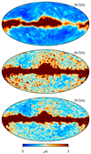 |
Fig. 5. Residual maps, rν, for each of the three Planck LFI frequencies, smoothed to a FWHM common angular resolution of 10°. |
We can see that these maps are then thresholded at values well above the noise level and these thresholded maps form the main input to the processing masks. Next, to remove particularly bright compact objects that may not be picked up by the smooth residual maps described above, we additionally remove all pixels with high free-free or AME levels (or both), as estimated in an earlier analysis. The final processing masks are shown in Fig. 6, and allow 73, 81, and 77% of the sky to be included while fitting correlated noise at 30, 44, and 70 GHz, respectively.
 |
Fig. 6. Processing masks used for correlated noise sampling. Different shades of gray indicate different frequency masks. The allowed 30 GHz sky fraction (light) is fsky = 0.73; the 44 GHz sky fraction (intermediate) is fsky = 0.81; and the 70 GHz sky fraction (dark) is fsky = 0.77. |
We note that while we use a processing mask when estimating the correlated noise, masking out data from high foreground signal regions, the data from these high signal regions are still used in the other parts of the BEYONDPLANCK pipeline (e.g., mapmaking, component separation, etc.). The difference is only that we have a more uncertain noise model in these regions (since the noise is extrapolated from outside and characterized by a high sample variance).
4.2. Degeneracies with the gain
The brightest component of the entire BEYONDPLANCK signal model is the Solar CMB dipole, which has an amplitude of 3 mK. This component plays a critical role in terms of gain estimation (Gjerløw et al. 2023) and serves as the main tool to determine relative calibration differences between detectors. Both the gain and CMB dipole parameters are of course intrinsically unknown quantities and must be fitted jointly. Any error in the determination of these will therefore necessarily result in a nonzero residual, in the same manner as Galactic foregrounds described above, and this may potentially also bias ncorr. Unlike the Galactic residuals, however, it is not possible to mask the CMB dipole, since it covers the full sky. The correlated noise component is therefore particularly susceptible to errors in either the gain or CMB dipole parameters, and residual large-scale dipole features in the binned ncorr map is a classic indication of calibration errors. To illustrate the effect of an incorrect gain model, Fig. 7 shows a 30 GHz correlated noise sample when assuming that the gain is constant throughout the entire Planck mission.
 |
Fig. 7. Correlated noise intensity sample for the 30 GHz band when fitting a model that assumes constant gains throughout the mission. This map has been smoothed to an angular resolution of 2.5° FWHM. |
The gain also has a direct connection with the white noise level, σ0. This is manifested in different ways, depending on the choice of units adopted for σ0. When expressed in units of volts, the white noise level is simply given by the radiometer equation:
![Mathematical equation: $$ \begin{aligned} \sigma _0 [\mathrm{V} ] \propto g_\mathrm{phys} T_\mathrm{sys} , \end{aligned} $$](/articles/aa/full_html/2023/07/aa43619-22/aa43619-22-eq42.gif) (26)
(26)
where gphys is the actual physical gain of the radiometer, and Tsys is the system temperature (BeyondPlanck Collaboration 2023). In calibrated units of KCMB, however, the white noise level is
![Mathematical equation: $$ \begin{aligned} \sigma _0 [\mathrm{K} ] \propto \frac{g_\mathrm{phys} }{g_\mathrm{model} }T_\mathrm{sys} , \end{aligned} $$](/articles/aa/full_html/2023/07/aa43619-22/aa43619-22-eq43.gif) (27)
(27)
where gmodel is the gain estimate in our model. When considering the evolution of the noise parameters as a function of time, we then note that σ0[V] will thus be correlated with the physical gain, which depends strongly on the thermal environment at any given time. On the other hand, if our gain model is correct, namely, gmodel ≈ gphys, these fluctuations will be canceled out in temperature units, and σ0[K] should instead correlate with the system temperature, Tsys. The system temperature also depends on the physical temperature, Tphys, as the amplifiers’ noise and waveguide losses increase with temperature. These were measured in pre-flight tests to be at a level dTsys/dTphys ≈ 0.2–0.5 K/K, depending on the radiometer (Terenzi et al. 2009). In conclusion, if we observe a sudden change in σ0[K] that is not present in σ0[V], this might indicate a problem in the gain model. We also expect that changes in σ0[K] reflect genuine variations of the white noise level, mainly driven by changes in the 20 K stage. In the following, we plot σ0 as a function of time in both units of volts and kelvins, and use these to disentangle gain and system temperature variations.
5. Results
Here, we present the main results obtained in applying the methods described above to the Planck LFI data within the BEYONDPLANCK Gibbs sampling framework (BeyondPlanck Collaboration 2023), as summarized in terms of the posterior distributions for each of the noise parameters. In total, four independent Gibbs chains were produced in the main BEYONDPLANCK analysis, each chain including 500–1000 samples, for a total computational cost of about 620 000 CPU-hours (BeyondPlanck Collaboration 2023; Galloway et al. 2023b).
5.1. Posterior distributions and Gibbs chains
First, we recall that at every step in the Gibbs chain, we sample the correlated noise parameters for each pointing period and each radiometer, both the time-domain realization ncorr and the PSD parameters ξn. To visually illustrate the resulting variations from sample to sample in terms of PSDs, Fig. 8 shows three subsequent spectrum samples for a single pointing period for the 23S radiometer. We see that the correlated noise follows the data closely at low frequencies, while at high frequencies the correlated noise is completely dominated by the sampling terms; thus, at these frequencies, the correlated noise PSD is effectively extrapolated based on the current noise PSD model. The scatter between the three colored curves shows the typical level of variations allowed by the combination of white noise and degeneracies with other parameters in the model.
 |
Fig. 8. Three subsequent samples (colored curves) of the correlated noise PSD for 23S, one of the 70 GHz radiometers. The black line shows the PSD of the signal-subtracted data. |
Figure 9 shows the pixel-space correlated noise corresponding to a single Gibbs sample, obtained after binning ncorr for all radiometers and all PIDs into an IQU map. The columns show different frequency maps (30, 44, and 70 GHz) and rows show different Stokes parameters (I, Q, and U). Overall, we see that the morphology of each map is dominated by stripes along the Planck scanning strategy, as expected for correlated 1/f noise, and we do not see any obvious signatures of either residual foregrounds in the Galactic plane, nor CMB dipole leakage at high latitudes. This suggests that the combination of the data model and processing masks described above performs reasonably well. We also note that the peak-to-peak values of the total correlated noise maps are 𝒪(1 μK), which is of the same order of magnitude as the predicted E-mode signal from cosmic reionization (Planck Collaboration IV 2020). Thus, correlated noise estimation plays a critical role for large-scale polarization reconstruction, while it is negligible for CMB temperature analysis.
 |
Fig. 9. Maps of a single Gibbs sample of the correlated noise added over all radiometers in the 30 GHz (left), 44 GHz (middle) and 70 GHz (right) bands. From top to bottom: Rows show Stokes I, Q, and U, respectively. Maps have been smoothed to a common angular resolution of 5° FWHM. |
For both ncorr and ξn, the main result of the BEYONDPLANCK pipeline are the full ensembles of Gibbs samples. These are too large to visualize in their entirety here, and are instead provided digitally6. In the following, we therefore focus on ξn. As an example, Fig. 10 displays one of the full Gibbs chains for two different PIDs for one radiometer from each LFI frequency band. We see that the Gibbs chains appear both stable and well behaved. Some chains have longer Markov chain autocorrelation lengths than others, as expected from their different levels of degeneracies both within the noise model itself, and between the noise and the signal or gain. In particular, the lognormal amplitude, Ap, shows a long autocorrelation time, due to the degeneracy with fknee and α. However, while the long autocorrelation times are not ideal, all the chains are converging and seem to explore the full range of the distributions. In any case, moving power between the lognormal and the 1/f components has no effect on the rest of the model. To account for burn-in, we removed the first 50 samples from each chain.
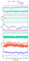 |
Fig. 10. Gibbs samples of noise parameters for two different PIDs for detectors 27M, 24S, and 20M of the 30, 44 and 70 GHz bands respectively. |
The main results are shown in Figs. 11–16, which summarize the noise PSD parameters for each LFI radiometer in terms of distributions of posterior means (top section; histograms made from the posterior means for all PIDs) and as average quantities as a function of PID (bottom section). The former are useful to obtain a quick overview of the mean behavior of a given radiometer, while the latter is useful to study its evolution in time. Blue, red, and green correspond to 30, 44, and 70 GHz radiometers, respectively. Mean ξn values are tabulated in Table 1, while the average noise properties of all radiometers in each band are plotted as a function of time in Fig. 17.
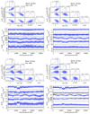 |
Fig. 11. Noise characterization of the Planck LFI 30 GHz radiometers; 27M (top left), 27S (top right); 28M (bottom left), and 28S (bottom right). For each radiometer, the top figure shows distributions of noise parameters PSD, ξn = {σ0, fknee, α, Ap}, averaged over all Gibbs samples for the full mission. The bottom figure shows the time evolution of the posterior mean of the noise parameters, and the bottom panel shows the evolution in reduced normalized χ2 in units of σ. Black dashed curves and crosses show corresponding values as derived by, and used in, the official Planck LFI DPC pipeline. |
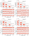 |
Fig. 12. Noise characterization of the Planck LFI 44 GHz radiometers; 24M (top left), 24S (top right); 25M (bottom left), and 25S (bottom right). For each radiometer, the top figure shows distributions of noise parameters PSD, ξn = {σ0, fknee, α, Ap}, averaged over all Gibbs samples for the full mission. The bottom figure shows the time evolution of the posterior mean of the noise parameters, and the bottom panel shows the evolution in reduced normalized χ2 in units of σ. Black dashed curves and crosses show corresponding values as derived by, and used in, the official Planck LFI DPC pipeline. |
 |
Fig. 13. Noise characterization of the Planck LFI 44 GHz radiometers; 26M (left), 26S (right). For each radiometer, the top figure shows distributions of noise parameters PSD, ξn = {σ0, fknee, α, Ap}, averaged over all Gibbs samples for the full mission. The bottom figure shows the time evolution of the posterior mean of the noise parameters, and the bottom panel shows the evolution in reduced normalized χ2 in units of σ. Black dashed curves and crosses show corresponding values as derived by, and used in, the official Planck LFI DPC pipeline. |
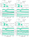 |
Fig. 14. Noise characterization of the Planck LFI 70 GHz radiometers; 18M (top left), 18S (top right); 19M (bottom left), and 19S (bottom right). For each radiometer, the top figure shows distributions of noise parameters PSD, ξn = {σ0, fknee, α}, averaged over all Gibbs samples for the full mission. The bottom figure shows the time evolution of the posterior mean of the noise parameters, and the bottom panel shows the evolution in reduced normalized χ2 in units of σ. Black dashed curves and crosses show corresponding values as derived by, and used in, the official Planck LFI DPC pipeline. |
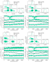 |
Fig. 15. Noise characterization of the Planck LFI 70 GHz radiometers; 20M (top left), 20S (top right); 21M (bottom left), and 21S (bottom right). For each radiometer, the top figure shows distributions of noise parameters PSD, ξn = {σ0, fknee, α}, averaged over all Gibbs samples for the full mission. The bottom figure shows the time evolution of the posterior mean of the noise parameters, and the bottom panel shows the evolution in reduced normalized χ2 in units of σ. Black dashed curves and crosses show corresponding values as derived by, and used in, the official Planck LFI DPC pipeline. |
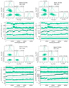 |
Fig. 16. Noise characterization of the Planck LFI 70 GHz radiometers; 22M (top left), 22S (top right); 23M (bottom left), and 23S (bottom right). For each radiometer, the top figure shows distributions of noise parameters PSD, ξn = {σ0, fknee, α}, averaged over all Gibbs samples for the full mission. The bottom figure shows the time evolution of the posterior mean of the noise parameters, and the bottom panel shows the evolution in reduced normalized χ2 in units of σ. Black dashed curves and crosses show corresponding values as derived by, and used in, the official Planck LFI DPC pipeline. |
 |
Fig. 17. Posterior mean noise parameters averaged over all radiometers in each band, for the full mission. |
Distribution of posterior mean noise parameters for each radiometer.
Regarding the mean values, we see that the 30 GHz radiometers generally have fairly high knee frequencies, fknee ∼ 100 mHz, and shallow power law slopes, α ∼ −0.85. The 70 GHz channels, on the other hand, have lower knee frequencies, fknee ∼ 20 mHz, and steeper slopes, α ∼ −1.2. The 44 GHz channels generally fall between these two extremes. The (normalized) 30 GHz amplitudes of the lognormal noise PSD component,  , are typically a bit larger, fluctuating between ∼0 − 1.5, than the 44 GHz ones, fluctuating between ∼0 − 0.7.
The values of α for the individual radiometers are, as expected, typically around −1, with a spread that depends on the detailed properties of each radiometer component. The intrinsic correlated noise is dominated by fluctuations in the gain and noise temperature of the FEM and BEM amplifiers, and on the isolation of the phase switches. In addition, common mode correlated noise is induced by temperature instabilities of the instrument interfaces (mainly in the 20 K and 300 K stages), with different amplitudes for different radiometers depending on their individual thermal susceptibility coefficient. All these noise contributions are then processed by the LFI pseudo-correlation scheme, which largely suppresses their effect in the scientific data by differencing the sky signal with the signal from the internal 4 K reference load, whose instabilities may, in principle, contribute to the correlated noise. A prediction of the combined effects of all these sources in terms of α and fknee of the differenced data for the individual radiometers is beyond the reach of our instrument model and those values can only be obtained by measurement.
The dashed lines in Figs. 11–16 show the Planck LFI DPC values for each parameter (Planck Collaboration II 2020), which are assumed to be constant throughout the mission. In most cases, these agree well with the results presented here. The main exception is the 30 GHz white noise level, σ0, for which we on average find values that are lower by about 2%. It is difficult to precisely pinpoint the origin of these differences, but we do note that Galactic foregrounds are particularly bright at 30 GHz. One possible hypothesis is that these are fitted slightly better in the joint and iterative BEYONDPLANCK approach, as compared to the linear pipeline DPC approach.
5.2. Time variability and goodness-of-fit tests
Perhaps the single most important and visually immediate conclusion to be drawn from these plots is the fact that the noise properties of the LFI instrument vary significantly in time. This is evident in all three frequency channels and all radiometers. Furthermore, by comparing the time evolution between different radiometers, we observe many common features, both between frequencies and, in particular, among radiometers within the same frequency band. Many of these may be associated with specific and known changes in the thermal environment of the satellite and can be traced using thermometer housekeeping data. This is the main topic for the next section.
The bottom panels in Figs. 11–16 show a χ2 per PID of the following form:
 (28)
(28)
where nsamp is the number of samples, and ri is the residual for sample i as defined by Eq. (25). Thus, this quantity measures the normalized mean-subtracted χ2 for each PID, which should, for ideal data and nsamp ≫ 1, be distributed according to a standard Gaussian distribution.
Starting with the 70 GHz channel, which is generally considered to be the most well behaved, we see that the χ2 fluctuates around zero for most channels, with a standard deviation of roughly unity. In general, the 30 and 44 GHz channels appear less stable than the 70 GHz channels in terms of overall χ2, with several detectors showing a positive bias of 1–2 σ per PID, with internal temporal variations at the 1 σ level. This suggests that while the addition of the lognormal noise PSD component certainly improves the fit of the noise PSD model, we still do not always get a perfect fit. This is not very surprising, since the shape parameters of the lognormal component are not chosen separately for each radiometer, only the overall amplitude is fit. Sampling the lognormal shape parameters independently for each radiometer is a main goal for future LFI analysis.
As a typical illustration of noise PSD model fits, Fig. 18 shows the PSD for a range of 18 PIDs for the 28M 30 GHz radiometer. Here the 1/f model is not able to fit the correlated noise to sufficient statistical accuracy at intermediate temporal frequencies, between 0.1 and 10 Hz, but rather shows a generally flatter trend. The addition of the lognormal component greatly improves the fit between about 0.3–3 Hz, but we still see significant deviations from the model at slightly lower frequencies this is an example of features that could be better fit if the shape parameters were fit individually for each radiometer. A similar behavior is seen in many 30 and 44 GHz radiometers, while the 70 GHz radiometers are better behaved.
 |
Fig. 18. PSD of signal-subtracted data from radiometer 28M, averaged over 18 PIDs (at intervals of 100 PIDs) in the range 30 000–32 000 (black). The dashed lines show the mean BEYONDPLANCK (dashed green) and LFI DPC (dashed and dotted gray) noise models for the same data. Dotted lines show the 1/f (blue) and lognormal (purple) components of the BEYONDPLANCK noise model. |
Turning our attention to the ξn parameters, we see much larger variability than in the χ2. First, we note a period of significant instability in most channels between PIDs 8000–20 000, but most strikingly in the 70 GHz α estimates. This feature is discussed in more detail in Sect. 6, where it is explicitly shown to be correlated with thermal variations. We note, however, that the noise model seems flexible enough to adjust to these particular changes, as no associated excess χ2 is observed in the same range.
Next, when considering the white noise level, σ0, given in units of volts or kelvins, we see the pattern anticipated in the previous section. The uncalibrated white noise in units of volts follows the slow drifts of the gain, which typically manifests itself in slow annual gain oscillations. In contrast, the calibrated noise in units of KCMB is far more stable. Other significant features include sharp jumps in noise properties, most notably seen around PID 20 000 for radiometer 26S (see Fig. 13), but also seen in most radiometers in the period before and after PID 11 000. Both of these aspects are discussed in Sect. 6.
6. Systematic effects
Previous LFI analyses have assumed a stationary noise model with three fixed parameters (σ0 [K], fknee, and α) for each of the 22 radiometers. In contrast, each of these parameters is estimated for every PID in BEYONDPLANCK increasing the total number of PSD noise parameters from 66 to more than 3 million. This increase in information allows us to capture the effects of evolution in the radiometer responses and local thermal environment, as well as subtle interactions between them. In this section, we use this new information to characterize potential residual systematic effects in the data, and, as far as possible, associate these with independent housekeeping data or known satellite events. An overview of the measurements from eight temperature sensors that are particularly important for LFI is provided in Fig. 19. For details on the locations of the various temperature sensors, we refer to Fig. 21 of Bersanelli et al. (2010) and Fig. 18 of Lamarre et al. (2010).
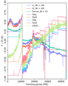 |
Fig. 19. High-level comparison of measurements from eight temperature sensors that are particularly relevant for LFI. Sensors TS5L, TS6L, TS1R, and TS2R are installed in the 20 K focal plane frame, while LVHX1 is the liquid-vapor heat exchanger providing 18 K to HFI; sensors L1_4K, L2_4K, and Cernox_4K are on the HFI 4 K stage supporting the LFI 4 K reference loads. The step-like increases in the 20 K stage are visible both before and after the sorption cooler switchover event (near PID 11 000). For details on the locations of the various temperature sensors, see Fig. 21 of Bersanelli et al. (2010) and Fig. 18 of Lamarre et al. (2010). For visualization purposes, the mean value has been subtracted from each data set, and some have been scaled by one or two orders of magnitude, as indicated in the legend. |
6.1. Temperature changes in the 20 K stage
A key element for the LFI thermal environment was the Planck sorption cooler system (SCS), which provided the 20 K stage to the LFI front-end and the 18 K pre-cooling stage to HFI. The SCS included a nominal and a redundant unit (Planck Collaboration II 2011). In August 2010 (around PID 11 000), a heat switch of the nominal cooler unit reached its end of life, and the SCS was therefore switched over to the redundant cooler7. This “switchover” event implied a major redistribution of the temperatures in the LFI focal plane, with variations at ∼1 K level, for two main reasons. First, the efficiency of the newly active redundant cooler led to an overall decrease of the absolute temperature. Second, because of the different location of the interface between the focal plane structure and the cold-end for the redundant cooler, a change of temperature gradients appeared across the focal plane.
Since the SCS dissipated significant power, changes in its configuration produced measurable thermal effects in the entire Planck spacecraft and most directly in the 20 K stage. In the period preceding the switchover, starting around PID 8000, a series of power input adjustments were commanded to reduce thermal fluctuations in the 20 K stage while optimizing the sorption cooler lifetime, which generated a number of step-like increases in the LFI focal plane temperature. These are measured by all of the LFI temperature sensors located in the 20 K focal plane unit, as shown in Fig. 19.
Following the switchover, in the period with PIDs 11 000–15 000, a significant increase of 20 K temperature fluctuations was observed. These excess fluctuations were understood as due to residual liquid hydrogen sloshing in the inactive cooler and affecting the cold-end temperature. The issue was resolved by heating the unit and letting the residual hydrogen evaporate. Afterwards, to optimize the performance and lifetime of the operating cooler, several periodic, step-like adjustments were again introduced in the operational parameters of the cooler. This resulted in a semi-gradual, monotonic increase of the LFI focal plane temperature from switchover to end of mission of ∼1.3 K.
In Fig. 19 the sudden discontinuity at switchover (PID 11 000) is visible for all temperature sensors, and the stepwise up-ward trend driven by SCS operational adjustments can be seen in all 20 K sensors. These temperature variations directly affected the LFI noise performance for most radiometers, as observed in the lower panels of Figs. 11–16. To see this, it may be useful to concentrate on a well-behaved case (e.g., radiometers 22 or 23, Fig. 16) and then recognize the same features in other radiometers.
The effect of the SCS switchover shows up as a sharp discontinuity also in the white noise levels near PID 11 000. The sudden decrease of the focal plane temperature of about 1 K implies a change in radiometer gain, as well as a genuine reduction in radiometer noise. This leads to a decrease not only in σ0 [V] but also σ0 [K]. Furthermore, due to the change in cold-end interface, the temperature drop at switchover was larger on the top-right-hand side of the focal plane (as defined by the view in Fig. 6 of BeyondPlanck Collaboration 2023) than in other regions. In particular, we see in Figs. 11–16 that the drop in σ0 [K] is particularly pronounced for radiometers 21, 22, 23, 27 (both M and S), which are all located in that portion of the focal plane.
Using Fig. 16 as a guide once again, we can also recognize the effect of the incremental increase of focal plane temperature due to sorption cooler adjustments, both before and after the switchover. The increasing physical temperature of the focal plane drives a corresponding increase of σ0 [K], which is visible for most of the radiometers in Figs. 11–16. However, we cannot exclude that part of the observed slow increase of white noise is due to aging effects degrading the intrinsic noise performance of the front-end amplifiers. To disentangle these two components would require a more detailed thermal and radiometric model.
6.2. Temperature fluctuations and 1/f parameters
In Fig. 20 (top four panels), we report the value and rms of representative temperature sensor of the 4 K and 20 K stages (L1_4K and TS5L). During the thermal instability period that followed the switchover, the noise properties of essentially all the 70 GHz radiometers markedly changed their 1/f noise behavior (with the only notable exception of 21M). This is highlighted in the lower two panels of Fig. 20, which show the averaged values of α and fknee for all the 70 GHz radiometers. The correlation between 1/f noise parameters and temperature fluctuations is very strong, with higher fluctuations producing an increase in fknee and a steepening (i.e., more negative) slope α. The latter is a typical behavior of thermally driven instabilities, which tend to transfer more power to low frequencies and thus steepen the 1/f tail. This behavior shows up also in the individual 70 GHz radiometers (Figs. 14–16).
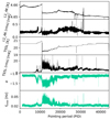 |
Fig. 20. Average correlated noise properties of the 70 GHz radiometers (bottom two panels) compared with 4 K and 20 K temperature sensor read-outs (top four panels) for the full mission. |
Figure 21 is a zoom into the pre-switchover period (PID 7000–11 000) of the upper plot. Here we see the effect of some of the step-wise adjustments in the sorption cooler operation, whose main effect is to temporarily reduce the temperature fluctuations. The observed tight correlation with the steepening of the slope is striking.
For a specific example of how noise property variations modify the noise PSD, Fig. 22 shows the average PSD for 10 PIDs between 3000–4000 (black) compared to 10 PIDs between 12 000–13 000 (grey) for the 70 GHz 20M radiometer. We see large increases in power at low frequencies, and a shift in the knee frequency.
 |
Fig. 22. PSD of signal subtracted data from radiometer 20M, averaged over 10 PIDs in the ranges 3000–4000 (black) and 12 000–13 000 (grey). |
These correlations also appear, albeit more weakly in the 30 and 44 GHz radiometers (see Fig. 17). In particular, there is no correlation with the knee frequency. This behavior could be partly explained by the fact that, by mechanical design, the front-end modules (FEMs) of the 30 and 44 GHz are less thermally coupled to the frame and cooler front-end; alternatively, it could be indicative of an additional source of non-thermal correlated noise that dominates the slope and knee frequency of these channels. This could be the case also for the 70 GHz radiometer 21M, for which the lack of correlation cannot be explained in terms of poor thermal coupling.
These hypotheses are supported by Fig. 18, which compares the PSD of the 30 GHz 28M signal-subtracted data, averaged over 18 PIDs in a typical stable period, with both the BEYONDPLANCK and LFI DPC noise models for the same period. We see that the 1/f model is not able to properly describe the observed data. The deviation indicates that there is an excess power in the frequency range between 0.1 and 5 Hz. This and similar excesses in many of the other 30 and 44 GHz channels are the motivation for adding the lognormal component to the noise model for these bands.
6.3. Seasonal effects and slow drifts
The changing Sun-satellite distance during the yearly Planck orbit around the Sun produced a seasonal modulation of the solar power absorbed by the spacecraft. The corresponding effect on the LFI thermal environment was negligible for the actively controlled front-end, as demonstrated by the lack of yearly modulation in the 20 K temperature sensors (see Fig. 19 and the upper panel of Fig. 20). However, the 300 K environment and the passive cooling elements (V-groove radiators) were affected by a ∼1% seasonal modulation (see Fig. 6 of Planck Collaboration I 2014).
Since the radiometer back-end modules (BEMs) provided a major contribution to the radiometer gain, g, and since they are located in the 300 K service module (SVM), the thermal susceptibility of the BEMs coupled with local thermal changes is expected to induce radiometer gain variations. On the other hand, since the BEMs are downstream relative to the > 30 dB amplification from the FEMs, their contribution to the noise temperature, Tsys, is negligible. Therefore we may expect the LFI uncalibrated signal (and the uncalibrated noise σ0 [V]) to show a seasonal modulation due to thermally-driven BEM gain variations, with essentially no degeneracy with Tsys.
Figures 11–16 show that several LFI radiometers exhibit such modulation in the uncalibrated white noise, σ0 [V], throughout the four year survey. For all of these, the modulation disappears in σ0 [K], indicating that our gain model properly captures this effect. We also observe that the sign of the modulation is opposite for the 70 GHz and the 30/44 GHz radiometers. Furthermore, all radiometers that exhibit seasonal modulation also show a systematic slow drift of σ0 [V] throughout the mission with the same sign as the initial modulation (which corresponds to increasing physical temperatures in the SVM). Since the spacecraft housekeeping recorded a slow overall increase in temperature throughout the mission (ΔT ≈ 5 K), the observed drift of σ0 [V] is qualitatively consistent with the hypothesis of BEM susceptibility as the origin of the effect.
For each radiometer, the amplitude of the modulation depends on the details of the thermal susceptibility of the LFI elements down-stream relative to the third V-groove, including waveguide losses, BEM components, particularly low-noise amplifiers (LNAs), detector diodes, data acquisition electronics (gain and offset), and so on. The dominant element is the BEM, whose thermal susceptibility was measured in the LFI pre-launch test campaign for the 30 and 44 GHz radiometers (Villa et al. 2010). The change in BEM output voltage, ΔVout, as a function of the variation in BEM physical temperature, ΔTBEM, can be written as:
 (29)
(29)
where Tin is the input signal temperature (either sky or reference load) and ϕBEM is a transfer function quantifying the BEM thermal susceptibility. The measured values of ϕBEM (Villa et al. 2010) were slightly negative for all the 30 and 44 GHz radiometers, ranging from −0.01 to −0.02, and this is consistent with both the observed overall drift and the seasonal effect. No such ground tests could be done for the 70 GHz instrument. However, in-flight tests during commissioning (Cuttaia & Terenzi 2011) revealed that the sign of ϕBEM for the 70 GHz radiometers was opposite to those of 30 and 44 GHz, which is consistent with our interpretation.
6.4. Inter-radiometer correlations
So far, we have mostly considered noise properties as measured separately for each radiometer. However, given the significant sensitivity to external environment parameters discussed above, it is also interesting to quantify the correlations between detectors. As a first measure of this, we plot in Fig. 23 the correlation of ncorr averaged over all pairs of radiometers within each frequency band as a function of PID. As expected from the previous discussion, we find a large common correlation for the 70 GHz channel that peaks in the post-switchover period. Similar coherent patterns are seen in the 30 and 44 GHz channels, but at somewhat lower levels.
 |
Fig. 23. Average correlation between the correlated noise in the different radiometers in each frequency band for the full mission. Colored dots indicate correlations found in a single PID, while the colored curves are a “running mean” of the corresponding points. We use every hundreth PID, so that 1% of all PIDs are included in the plot. |
As a specific example of such common mode noise, Fig. 24 shows the signal subtracted timestreams for one radiometer from each band for PID 12 301, which is representative for the period of maximum correlation. Here, we see that the same large scale fluctuations are present in all three bands, though at different levels of amplitude. In Fig. 25 we show the average cross-correlation between time streams of all 70 GHz radiometers for the same PID. We compare the average correlation between the correlated noise components, ncorr, with the correlation between the residuals,  . We see that even though the correlations between the ncorr components are large, the residuals are highly uncorrelated. This is an indication that the common mode signal is efficiently described by ncorr, and it therefore does not leak into the rest of the BEYONDPLANCK pipeline.
 |
Fig. 24. Signal subtracted data from radiometers from all three bands for PID 12 301. The data is averaged over a 20 second timescale and scaled to fit in the same plot. |
 |
Fig. 25. Average cross-correlation between timestreams of all 70 GHz radiometers for PID 12301. Orange points show average correlation between the correlated noise components, while the grey points shows average correlation between the residuals. We see that even though the correlation between the correlated noise components is high, the residuals are completely uncorrelated, indicating that this correlated signal does not leak into the rest of the pipeline and, rather, it is incorporated into the correlated noise. |
Figure 26 shows a global correlation matrix of all the noise parameters for all the LFI radiometers throughout the mission. A number of interesting features can be recognized in this diagram:
 |
Fig. 26. Noise parameter correlation matrix. We average over all Gibbs samples of the noise parameters, ξn = {σ0, fknee, α, Ap}, for each PID. We then find the correlation in time between these averages for the different bands and detectors. The results here are for the calibrated white noise level, σ0 [K]. |
First, we note that all 70 GHz radiometers exhibit an internally coherent trend, where fknee and α behave essentially as a common mode for the entire 70 GHz array, with the only exception being 21M. This coherent behavior reflects the common thermal origin of the 1/f noise of the 70 GHz radiometers, as discussed in Sect. 6.2. We also see that σ0 [K] shows a similar common mode behavior for the 70 GHz radiometers and, to a lesser extent, it also correlates with the σ0 [K] of the 30 and 44 GHz radiometers. This is indicative of the fact that changes in the LFI radiometers’ sensitivities are driven by the global LFI thermal environment, most importantly by the slow increase in temperature at the 20 K temperature stage.
However, for 30 and 44 GHz, we do not observe the same common mode behavior for fknee and α as for the 70 GHz. Rather, we see positive correlation (red pixels in Fig. 26) between fknee and α within each single radiometer. This suggests that (a) the dominant source of 1/f noise is independent for each 30 and 44 GHz radiometer and (b) for a given radiometer, as fknee increases, the slope becomes flatter (i.e., α becomes less negative). This behavior further supports the hypothesis that the dominant source of correlated noise in the 30 and 44 GHz is not of thermal origin.
We see that the amplitude of the lognormal noise component, Ap, is negatively correlated with both α and fknee. This makes sense, since with the lognormal component added, α and fknee no longer have to adjust to the intermediate frequency noise signal, which means that fknee is lower and α gets steeper.
Finally, we observe an anti-correlation between fknee and σ0 (as a common mode at 70 GHz and individually for 30 and 44 GHz). Slightly larger values of fknee for lower σ0 can be understood in terms of the correlated fluctuations becoming subdominant near fknee when the white noise increases during the mission time.
6.5. Correlation with housekeeping data
Next, we correlated the LFI noise parameters with housekeeping data – in particular with temperature sensors that are relevant for LFI. This process is summarized in Fig. 27, showing the correlation coefficients with respect to several sensors that monitor the 20 K stage (TS5L, TS2R, TS6L, TS1R, LVHX1) and the 4 K stage (L1_4K, L2_4K, Cernox_4K). Some significant patterns appear that can be interpreted in terms of the general instrument behavior: (1) For the 70 GHz radiometers, both the rms and the peak-to-peak variations of the 20 K temperature sensor fluctuations are correlated with fknee and anti-correlate with α (i.e., they prefer a steeper power-law slope). This indicates that the 1/f noise of the 70 GHz radiometers is dominated by residual thermal fluctuations in the 20 K stage. A similar trend can be seen also at 30 GHz in the two horn-coupled receivers 28M and 28S. However, the 44 GHz channels show no sign of this behavior. Combined with the lack of correlation with the 4 K sensors, this is consistent with the hypothesis that the 1/f noise of the 44 GHz (and partly the 30 GHz) radiometers is dominated by non-thermal fluctuations. (2) Weaker correlations are seen between the various noise parameters and the 4 K temperature sensors. The lack of significant correlation of the rms and peak-to-peak variations of 4 K sensors with any of the 1/f parameters, fknee and α, is an indication that the 4 K reference loads do not contribute significantly to the radiometers correlated noise. (3) Strong anti-correlation (correlation) of the gain g with the absolute value of the 20 K sensors for the 70 GHz (30/44 GHz) radiometers is observed. Based on the discussion in Sect. 6.3, this pattern can be understood by noting that the 20 K stage temperature systematically increased throughout the mission, driven by sorption cooler adjustments. The same monotonic trend was also on-going in the 300 K stage, which controls the BEM amplifiers. This is thus a spurious correlation, for which the increasing back-end temperature actually leads to lower (higher) values of g for the 70 GHz (30/44 GHz) radiometers.
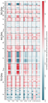 |
Fig. 27. Correlation in time, for the complete mission, between noise parameters and the temperature sensors. For each sensor we show the results (from left to right) from the mean temperature, the temperature rms, and the peak-to-peak temperature of each sensor within each pointing period. The results here are for the calibrated white noise level, σ0 [K]. We have imposed a mild high-pass filter (in time) of the different datasets in order to avoid random correlations on the very longest timescales. |
6.6. Issues with individual radiometers
In addition to the overall behavior and correlations that are common to many or most radiometers, there are issues that only seem to affect individual radiometers. Here, we point out two special cases: 26S and 21M.
First, as discussed above, we often find excess noise power in the 30 and 44 GHz channels in the signal-subtracted data at intermediate frequencies, ∼0.01–5 Hz, which cannot be described with a 1/f noise model. The most extreme example of this is the 44 GHz 26S radiometer, as shown in the bottom panel of Fig. 13. Here we see a jump in fknee around PID 20 800, after which the noise parameters change abruptly. This is elucidated in Fig. 28, which compares the noise PSD averaged over 10 PIDs in the 12 000–13 000 range with a corresponding average evaluated in the 32 000–33 000 range. We see that the signal from the early period is consistent with a 1/f spectrum, while for the later period we find an excess in power at intermediate frequencies that is not possible to fit with the 1/f noise model. Considering that the Planck spin period is 60 s, temporal frequencies of 0.1–1 Hz correspond to angular scales of 6–60° on the sky. This noise excess therefore represents a significant contaminant with respect to large-scale CMB polarization reconstruction, which is one of the main scientific targets for the current BEYONDPLANCK analysis. This is why the lognormal component was added, that is, to prevent this excess noise from leaking into any of the sky components or other parts of our model.
 |
Fig. 28. PSD of signal subtracted data from radiometer 26S, averaged over ten PIDs (at intervals of 100 PIDs) in the ranges 12 000–13 000 (black) and 32 000–33 000 (grey). We see that there is significantly more power in the frequency range 0.1–10 Hz in the later period. |
The sudden degradation of 26S at around PID 21 000 has no simultaneous counterpart in any other LFI radiometer, including the coupled 26M which exhibits a normal behavior (see Fig. 13). This suggests a singular event within the 26S itself, or in the bias circuits serving its RF components. Since we do not observe any significant changes in the radiometer output signal level and no anomalies are seen in the LNAs currents, it is unlikely that the problem resides in the HEMT amplifiers. A more plausible cause would be a degradation of the phase switch performance, possibly due to aging, the instability of the input currents, or a loss of internal tuning balance (Mennella et al. 2010; Cuttaia et al. 2009). Indeed sub-optimal operation of the phase switches would not significantly change the signal output level, but is known to introduce excess 1/f noise, as verified during the ground testing and in-flight commissioning phase.
The second anomalous case is the 70 GHz 21M radiometer. While the noise properties of the other 70 GHz channels are (internally) significantly correlated, this particular channel does not show similar correlations. The reason for the different behavior of 21M is still not fully understood. However, as shown for PID 2201 in Fig. 29, this particular radiometer exhibits a typical “popcorn” or “random telegraph” noise, that is, a white noise jumping between two different offset states. During ground testing this behavior was noted in the undifferenced data of LFI21 and LFI23 and ascribed to bimodal instability in the detector diodes. The effect was then recognized in-flight and this prevented any proper correction of ADC nonlinearity effect (Planck Collaboration III 2014). However, because the timescale of diode jumps between states (typically a few minutes) is longer than the differencing between sky and reference load (0.25 ms, corresponding to the phase switch frequency of 4 kHz), the effect can be efficiently removed in the differenced data. In the current analysis, we actually observe popcorn behavior in the differenced data, suggesting either an increased instability of the affected diode in 21M (possibly due to aging) or an alternative origin for the effect. Popcorn noise has been also found in some HFI channels (Planck HFI Core Team 2011). We have not seen any sign of popcorn noise in any of the other LFI channels besides 21M, but we did not perform a deep dedicated search for it. Nonetheless, the fact that the χ2 distribution for channel 21M appears acceptable suggests that this effect, even if it manages to survive in the differenced data stream, occurs at a sufficiently long timescale, such that ncorr is able to absorb it, preventing it from leaking into other astrophysical components.
 |
Fig. 29. Signal subtracted data from radiometer 21M for PID 2201. The data are averaged over a one second timescale. |
7. Conclusions
This paper has two main goals. First, it aims to describe Bayesian noise estimation within a global CMB analysis framework (BeyondPlanck Collaboration 2023). As such, this work represents the first real-world application and demonstration of methods originally introduced by Wehus et al. (2012). At the same time, this study takes advantage of important numerical improvements introduced by Keihänen et al. (2023). The second main goal is to apply this method to the Planck LFI measurements to characterize their noise properties to a more detailed extent than done previously (Planck Collaboration II 2020).
An important question regarding the original work of Wehus et al. (2012) was whether the method would be practical for real-world observations or whether it was too computationally expensive to be useful in a real pipeline. We are now in a position to quantitatively answer this question. As summarized by BeyondPlanck Collaboration (2023), Galloway et al. (2023b), the noise estimation step in the BEYONDPLANCK pipeline accounts for 19% of the total runtime (27 CPU-hours per sample for the 70 GHz channel), most of which is spent Fourier transforming the raw time-ordered data. As such, exact Bayesian noise estimation certainly is an expensive pipeline component – but it is by no means prohibitive. Additionally, it is important to note that Bayesian correlated noise sampling replaces both traditional mapmaking and noise covariance matrix evaluations (Keihänen et al. 2023; Suur-Uski et al., in prep.), which are two of the most expensive procedures in a traditional CMB analysis pipeline (Planck Collaboration I 2020) and, in fact, this leads to lower computational requirements overall. As an example, we note that a full BEYONDPLANCK Gibbs sample (which includes both low- and high-level processing with all LFI channels) costs 243 CPU-hours, while producing a single component of the Planck Full Focal Plane (FFP) simulation of the 70 GHz channel costs 9360 CPU-hours (Planck Collaboration XII 2016). Likewise, we also note that the current BEYONDPLANCK analysis was run on an in-house cluster with 256 cores and 4 TB of RAM, while the Planck simulations were produced on a large national computing center with 𝒪(105) cores (Planck Collaboration I 2020; Planck Collaboration Int. LVII 2020). We believe that the computational speed of this method alone should make it an attractive option for other CMB experiments, not to mention the possibilities of performing joint exact Bayesian analysis.
As far as LFI-specific analyses are concerned, the current results point toward generally complex noise behavior with subtle contributions from origins that have not yet been fully accounted for. Most notably, the noise properties of each LFI radiometer vary significantly in time and acutely depend on the thermal environment of the instrument. For the 70 GHz channel, for which the correlated noise amplitude (and knee frequency) is generally low, most of these variations may be described in terms of a simple 1/f model with time-dependent parameters. With very few exceptions, the time-domain χ2 of this channel is statistically acceptable throughout the mission.
However, for the 30 and 44 GHz channels, a more complex picture has emerged. Multiple observations suggest an as-yet unexplained source of non-thermal correlated noise in the 44 GHz (and at a lower level in the 30 GHz radiometers) that is responsible for mild (and possibly time-varying) deviations from the simple 1/f model. Inspection of individual PIDs indicates the presence of excess power between 0.1 and 5 Hz, well above the Planck scanning frequency of 0.017 Hz, thereby affecting the angular scales that are relevant for large-scale CMB polarization science. This excess motivated the addition of a lognormal noise component, at intermediate frequencies, in addition to the 1/f component for these bands.
Our analysis suggests that these effects are not due to temperature fluctuations, but they are, rather, associated with other effects, such as electrical instabilities or other environmental issues. We carried out a preliminary investigation by correlating the LFI radiometers whose LNA bias were supplied by common electronics groups8, but we have found no compelling evidence of correlations or anomalies. Many other electrical effects must be studied by exploiting all the available housekeeping information. Most of the spikes in the rms of the temperature sensors (see, e.g., Fig. 20) are readily understood to be attributed to commanded cooler adjustments, but a few of them deserve further investigation. The influence of transient perturbations should also be systematically investigated, including the possible effect of cosmic rays and solar flares.
A complete and quantitative analysis requires a detailed thermal model of the full instrument that includes the back-end unit and interfaces with the V-grooves, coupled with thermal susceptibility parameters of the relevant components (LNAs, OMTs, waveguides, BEMs, detector diodes, and data acquisition electronics). Such a detailed study is beyond the scope of this work, but this will now be possible in the near future thanks to the present study.
It is important to note that while we have focused this discussion on the application to the LFI time-ordered-data, the methods presented here are much more general. As the addition of the lognormal noise component shows, the methods can accomodate any parametric noise PSD model, as long as the data can constrain it. It can also be straightforwardly extended to cases where we have correlated noise components that are common to several detectors, which is, for instance, typically the case for atmospheric fluctuations.
In general, the detailed BEYONDPLANCK modeling approach allows us to highlight a number of subtle systematic patterns in the LFI radiometers that were previously noted and reported in earlier analyses. However, it is only now, for the first time, that it has become possible to elucidate and understand in greater detail. The examples featured here provide a detailed characterization of the nature of seasonal modulations and long term drifts, correlations between instrument noise parameters and temperature sensor read-out information, and deviations from the 1/f noise model. These methods are likely to play a central role in the analysis of future high-sensitivity CMB B-mode experiments such as LiteBIRD (Sugai et al. 2020; LiteBIRD Collaboration 2023).
Each pair of radiometers are connected to the same feedhorn through the main arm (M) or side arm (S) of an orthomode transducer, and are therefore sensitive to orthogonal linear polarizations.
The white noise levels σ0 are specified for an integration time corresponding to three samples per FWHM beam crossing (see Maris et al. 2009 for details); σ0 has different units if we are discussing the uncalibrated data, σ0 [V], calibrated data, σ0 [K] ≡σ0 [V] /g, or the white noise PSD,  [K2 Hz−1] ≡(σ0 [K]
 , where Rsamp is the sample rate (in Hz) of the time ordered data. Where this distinction is important, we include the units explicitly.
When a parameter appears on the right-hand side of a conditioning bar in a probability distribution, it is assumed known to infinite precision. It is therefore for the moment a constant quantity, and not associated with any stochastic degrees of freedom or uncertainties.
We use the FFTW library, in which case  , where nsamples is the number of time samples.
The residual used here is based on a preliminary test run, since these masks are used internally in the final analysis.
This operation took place at PID 10911, corresponding to Operation Day (OD) 454.
There were four such power groups in LFI, feeding the radiometers associated with the following horn sets: (19-20-28), (18-26), (21-22-24-27), (23-25).
Acknowledgments
We thank Prof. Pedro Ferreira and Dr. Charles Lawrence for useful suggestions, comments and discussions. We also thank the entire Planck and WMAP teams for invaluable support and discussions, and for their dedicated efforts through several decades without which this work would not be possible. The current work has received funding from the European Union’s Horizon 2020 research and innovation programme under grant agreement numbers 776282 (COMPET-4; BEYONDPLANCK), 772253 (ERC; BITS2COSMOLOGY), and 819478 (ERC; COSMOGLOBE). In addition, the collaboration acknowledges support from ESA; ASI and INAF (Italy); NASA and DoE (USA); Tekes, Academy of Finland (grant no. 295113), CSC, and Magnus Ehrnrooth foundation (Finland); RCN (Norway; grant nos. 263011, 274990); and PRACE (EU).
References
- Abazajian, K., Addison, G., Adshead, P., et al. 2019, ArXiv e-prints [arXiv:1907.04473] [Google Scholar]
- Ade, P., Aguirre, J., Ahmed, Z., et al. 2019, JCAP, 2019, 056 [Google Scholar]
- Andersen, K. J., Herman, D., Aurlien, R., et al. 2023, A&A, 675, A13 (BeyondPlanck SI) [NASA ADS] [CrossRef] [EDP Sciences] [Google Scholar]
- Ashdown, M. A. J., Baccigalupi, C., Balbi, A., et al. 2007, A&A, 471, 361 [NASA ADS] [CrossRef] [EDP Sciences] [Google Scholar]
- Bennett, C. L., Larson, D., Weiland, J. L., et al. 2013, ApJS, 208, 20 [Google Scholar]
- Bersanelli, M., Mandolesi, N., Butler, R. C., et al. 2010, A&A, 520, A4 [NASA ADS] [CrossRef] [EDP Sciences] [Google Scholar]
- BeyondPlanck Collaboration (Andersen, K. J., et al.) 2023, A&A, 675, A1 (BeyondPlanck SI) [Google Scholar]
- Bond, J. R., Jaffe, A. H., & Knox, L. 2000, ApJ, 533, 19 [NASA ADS] [CrossRef] [Google Scholar]
- Colombo, L. P. L., Eskilt, J. R., Paradiso, S., et al. 2023, A&A, 675, A11 (BeyondPlanck SI) [NASA ADS] [CrossRef] [EDP Sciences] [Google Scholar]
- Cuttaia, F., & Terenzi, L. 2011, Planck-LFI Technical Note, 098 [Google Scholar]
- Cuttaia, F., Mennella, A., Stringhetti, L., et al. 2009, J. Instrum., 4, 2013 [Google Scholar]
- Galloway, M., Andersen, K. J., Aurlien, R., et al. 2023a, A&A, 675, A3 (BeyondPlanck SI) [NASA ADS] [CrossRef] [EDP Sciences] [Google Scholar]
- Galloway, M., Reinecke, M., Andersen, K. J., et al. 2023b, A&A, 675, A8 (BeyondPlanck SI) [NASA ADS] [CrossRef] [EDP Sciences] [Google Scholar]
- Gjerløw, E., Ihle, H. T., Galeotta, S., et al. 2023, A&A, 675, A7 (BeyondPlanck SI) [NASA ADS] [CrossRef] [EDP Sciences] [Google Scholar]
- Gorski, K. M. 1994, ApJ, 430, L85 [NASA ADS] [CrossRef] [Google Scholar]
- Hanany, S., Alvarez, M., Artis, E., et al. 2019, ArXiv e-prints [arXiv:1902.10541] [Google Scholar]
- Hivon, E., Górski, K. M., Netterfield, C. B., et al. 2002, ApJ, 567, 2 [NASA ADS] [CrossRef] [Google Scholar]
- Keihänen, E., Suur-Uski, A.-S., Andersen, K. J., et al. 2023, A&A, 675, A2 (BeyondPlanck SI) [NASA ADS] [CrossRef] [EDP Sciences] [Google Scholar]
- Lamarre, J., Puget, J., Ade, P. A. R., et al. 2010, A&A, 520, A9 [NASA ADS] [CrossRef] [EDP Sciences] [Google Scholar]
- Lewis, A., & Bridle, S. 2002, Phys. Rev. D, 66, 103511 [Google Scholar]
- LiteBIRD Collaboration (Allys, E., et al.) 2023, Prog. Theor. Exp. Phys, 2023, 042F01 [CrossRef] [Google Scholar]
- Maris, M., Tomasi, M., Galeotta, S., et al. 2009, J. Instrum., 4, 2018 [Google Scholar]
- Mennella, A., Bersanelli, M., Butler, R. C., et al. 2010, A&A, 520, A5 [NASA ADS] [CrossRef] [EDP Sciences] [Google Scholar]
- Page, L., Hinshaw, G., Komatsu, E., et al. 2007, ApJS, 170, 335 [Google Scholar]
- Paradiso, S., Colombo, L. P. L., Andersen, K. J., et al. 2023, A&A, 675, A12 (BeyondPlanck SI) [NASA ADS] [CrossRef] [EDP Sciences] [Google Scholar]
- Planck HFI Core Team 2011, A&A, 536, A4 [NASA ADS] [CrossRef] [EDP Sciences] [Google Scholar]
- Planck Collaboration I. 2011, A&A, 536, A1 [NASA ADS] [CrossRef] [EDP Sciences] [Google Scholar]
- Planck Collaboration II. 2011, A&A, 536, A2 [NASA ADS] [CrossRef] [EDP Sciences] [Google Scholar]
- Planck Collaboration I. 2014, A&A, 571, A1 [NASA ADS] [CrossRef] [EDP Sciences] [Google Scholar]
- Planck Collaboration II. 2014, A&A, 571, A2 [NASA ADS] [CrossRef] [EDP Sciences] [Google Scholar]
- Planck Collaboration III. 2014, A&A, 571, A3 [NASA ADS] [CrossRef] [EDP Sciences] [Google Scholar]
- Planck Collaboration II. 2016, A&A, 594, A2 [NASA ADS] [CrossRef] [EDP Sciences] [Google Scholar]
- Planck Collaboration XII. 2016, A&A, 594, A12 [NASA ADS] [CrossRef] [EDP Sciences] [Google Scholar]
- Planck Collaboration I. 2020, A&A, 641, A1 [NASA ADS] [CrossRef] [EDP Sciences] [Google Scholar]
- Planck Collaboration II. 2020, A&A, 641, A2 [NASA ADS] [CrossRef] [EDP Sciences] [Google Scholar]
- Planck Collaboration III. 2020, A&A, 641, A3 [NASA ADS] [CrossRef] [EDP Sciences] [Google Scholar]
- Planck Collaboration IV. 2020, A&A, 641, A4 [NASA ADS] [CrossRef] [EDP Sciences] [Google Scholar]
- Planck Collaboration V. 2020, A&A, 641, A5 [NASA ADS] [CrossRef] [EDP Sciences] [Google Scholar]
- Planck Collaboration VI. 2020, A&A, 641, A6 [NASA ADS] [CrossRef] [EDP Sciences] [Google Scholar]
- Planck Collaboration Int. LVII. 2020, A&A, 643, A42 [NASA ADS] [CrossRef] [EDP Sciences] [Google Scholar]
- QUIET Collaboration (Bischoff, C., et al.) 2011, ApJ, 741, 111 [NASA ADS] [CrossRef] [Google Scholar]
- Sugai, H., Ade, P. A. R., Akiba, Y., et al. 2020, J. Low Temp. Phys., 199, 1107 [CrossRef] [Google Scholar]
- Suzuki, A., Ade, P. A. R., Akiba, Y., et al. 2018, J. Low Temp. Phys., 193, 1048 [NASA ADS] [CrossRef] [Google Scholar]
- Svalheim, T. L., Zonca, A., Andersen, K. J., et al. 2023a, A&A, 675, A9 (BeyondPlanck SI) [NASA ADS] [CrossRef] [EDP Sciences] [Google Scholar]
- Svalheim, T. L., Andersen, K. J., Aurlien, R., et al. 2023b, A&A, 675, A14 (BeyondPlanck SI) [NASA ADS] [CrossRef] [EDP Sciences] [Google Scholar]
- Tegmark, M. 1997, ApJ, 480, L87 [NASA ADS] [CrossRef] [Google Scholar]
- Tegmark, M., Taylor, A. N., & Heavens, A. F. 1997, ApJ, 480, 22 [NASA ADS] [CrossRef] [Google Scholar]
- Terenzi, L., Salmon, M. J., Colin, A., et al. 2009, J. Instrum., 4, 2012 [Google Scholar]
- Villa, F., Terenzi, L., Sandri, M., et al. 2010, A&A, 520, A6 [NASA ADS] [CrossRef] [EDP Sciences] [Google Scholar]
- Wandelt, B. D., Larson, D. L., & Lakshminarayanan, A. 2004, Phys. Rev. D, 70, 083511 [Google Scholar]
- Wehus, I. K., Næss, S. K., & Eriksen, H. K. 2012, ApJS, 199, 15 [NASA ADS] [CrossRef] [Google Scholar]
All Tables
All Figures
 |
Fig. 1. Illustration of three constrained correlated noise realizations (colored curves) drawn from P(ncorr ∣ d, ξn, stot, g) for the Planck 30 GHz data (grey curve). Regions for which parts of the data have been masked, either due to a processing mask or flagged data, are marked as white gaps. |
| In the text | |
 |
Fig. 2. Correlated noise realizations using linear gap-filling (black) and full constrained realizations using CG (colored dashed lines) for simulated data with extreme noise properties and a large gap. This illustrates the limitation of the linear gap-filling procedure. In general, the linear gap-filling procedure tends to underestimate the fluctuations in ncorr on long timescales within the gaps. |
| In the text | |
 |
Fig. 3. Comparison of temporal PSDs for different components. The blue curve shows the PSD of the signal-subtracted data; the orange curve shows the fitted correlated noise PSD; and the gray line shows the PSD of the residual TOD. The dashed curves correspond to the best fit 1/f-noise model, with (blue) and without (orange) white noise. Note: The 70 GHz channels do not have a lognormal component. |
| In the text | |
 |
Fig. 4. Distribution of noise parameters for PID 3401 of radiometer 20M, one of the 70 GHz channels, for fixed stot and g. Dashed red lines correspond to results obtained without an active prior, while the solid line corresponds to results after including the active priors on fknee and α from Eqs. (23) and (24). The black cross indicates the best fit values derived by the DPC pipeline for this radiometer. |
| In the text | |
 |
Fig. 5. Residual maps, rν, for each of the three Planck LFI frequencies, smoothed to a FWHM common angular resolution of 10°. |
| In the text | |
 |
Fig. 6. Processing masks used for correlated noise sampling. Different shades of gray indicate different frequency masks. The allowed 30 GHz sky fraction (light) is fsky = 0.73; the 44 GHz sky fraction (intermediate) is fsky = 0.81; and the 70 GHz sky fraction (dark) is fsky = 0.77. |
| In the text | |
 |
Fig. 7. Correlated noise intensity sample for the 30 GHz band when fitting a model that assumes constant gains throughout the mission. This map has been smoothed to an angular resolution of 2.5° FWHM. |
| In the text | |
 |
Fig. 8. Three subsequent samples (colored curves) of the correlated noise PSD for 23S, one of the 70 GHz radiometers. The black line shows the PSD of the signal-subtracted data. |
| In the text | |
 |
Fig. 9. Maps of a single Gibbs sample of the correlated noise added over all radiometers in the 30 GHz (left), 44 GHz (middle) and 70 GHz (right) bands. From top to bottom: Rows show Stokes I, Q, and U, respectively. Maps have been smoothed to a common angular resolution of 5° FWHM. |
| In the text | |
 |
Fig. 10. Gibbs samples of noise parameters for two different PIDs for detectors 27M, 24S, and 20M of the 30, 44 and 70 GHz bands respectively. |
| In the text | |
 |
Fig. 11. Noise characterization of the Planck LFI 30 GHz radiometers; 27M (top left), 27S (top right); 28M (bottom left), and 28S (bottom right). For each radiometer, the top figure shows distributions of noise parameters PSD, ξn = {σ0, fknee, α, Ap}, averaged over all Gibbs samples for the full mission. The bottom figure shows the time evolution of the posterior mean of the noise parameters, and the bottom panel shows the evolution in reduced normalized χ2 in units of σ. Black dashed curves and crosses show corresponding values as derived by, and used in, the official Planck LFI DPC pipeline. |
| In the text | |
 |
Fig. 12. Noise characterization of the Planck LFI 44 GHz radiometers; 24M (top left), 24S (top right); 25M (bottom left), and 25S (bottom right). For each radiometer, the top figure shows distributions of noise parameters PSD, ξn = {σ0, fknee, α, Ap}, averaged over all Gibbs samples for the full mission. The bottom figure shows the time evolution of the posterior mean of the noise parameters, and the bottom panel shows the evolution in reduced normalized χ2 in units of σ. Black dashed curves and crosses show corresponding values as derived by, and used in, the official Planck LFI DPC pipeline. |
| In the text | |
 |
Fig. 13. Noise characterization of the Planck LFI 44 GHz radiometers; 26M (left), 26S (right). For each radiometer, the top figure shows distributions of noise parameters PSD, ξn = {σ0, fknee, α, Ap}, averaged over all Gibbs samples for the full mission. The bottom figure shows the time evolution of the posterior mean of the noise parameters, and the bottom panel shows the evolution in reduced normalized χ2 in units of σ. Black dashed curves and crosses show corresponding values as derived by, and used in, the official Planck LFI DPC pipeline. |
| In the text | |
 |
Fig. 14. Noise characterization of the Planck LFI 70 GHz radiometers; 18M (top left), 18S (top right); 19M (bottom left), and 19S (bottom right). For each radiometer, the top figure shows distributions of noise parameters PSD, ξn = {σ0, fknee, α}, averaged over all Gibbs samples for the full mission. The bottom figure shows the time evolution of the posterior mean of the noise parameters, and the bottom panel shows the evolution in reduced normalized χ2 in units of σ. Black dashed curves and crosses show corresponding values as derived by, and used in, the official Planck LFI DPC pipeline. |
| In the text | |
 |
Fig. 15. Noise characterization of the Planck LFI 70 GHz radiometers; 20M (top left), 20S (top right); 21M (bottom left), and 21S (bottom right). For each radiometer, the top figure shows distributions of noise parameters PSD, ξn = {σ0, fknee, α}, averaged over all Gibbs samples for the full mission. The bottom figure shows the time evolution of the posterior mean of the noise parameters, and the bottom panel shows the evolution in reduced normalized χ2 in units of σ. Black dashed curves and crosses show corresponding values as derived by, and used in, the official Planck LFI DPC pipeline. |
| In the text | |
 |
Fig. 16. Noise characterization of the Planck LFI 70 GHz radiometers; 22M (top left), 22S (top right); 23M (bottom left), and 23S (bottom right). For each radiometer, the top figure shows distributions of noise parameters PSD, ξn = {σ0, fknee, α}, averaged over all Gibbs samples for the full mission. The bottom figure shows the time evolution of the posterior mean of the noise parameters, and the bottom panel shows the evolution in reduced normalized χ2 in units of σ. Black dashed curves and crosses show corresponding values as derived by, and used in, the official Planck LFI DPC pipeline. |
| In the text | |
 |
Fig. 17. Posterior mean noise parameters averaged over all radiometers in each band, for the full mission. |
| In the text | |
 |
Fig. 18. PSD of signal-subtracted data from radiometer 28M, averaged over 18 PIDs (at intervals of 100 PIDs) in the range 30 000–32 000 (black). The dashed lines show the mean BEYONDPLANCK (dashed green) and LFI DPC (dashed and dotted gray) noise models for the same data. Dotted lines show the 1/f (blue) and lognormal (purple) components of the BEYONDPLANCK noise model. |
| In the text | |
 |
Fig. 19. High-level comparison of measurements from eight temperature sensors that are particularly relevant for LFI. Sensors TS5L, TS6L, TS1R, and TS2R are installed in the 20 K focal plane frame, while LVHX1 is the liquid-vapor heat exchanger providing 18 K to HFI; sensors L1_4K, L2_4K, and Cernox_4K are on the HFI 4 K stage supporting the LFI 4 K reference loads. The step-like increases in the 20 K stage are visible both before and after the sorption cooler switchover event (near PID 11 000). For details on the locations of the various temperature sensors, see Fig. 21 of Bersanelli et al. (2010) and Fig. 18 of Lamarre et al. (2010). For visualization purposes, the mean value has been subtracted from each data set, and some have been scaled by one or two orders of magnitude, as indicated in the legend. |
| In the text | |
 |
Fig. 20. Average correlated noise properties of the 70 GHz radiometers (bottom two panels) compared with 4 K and 20 K temperature sensor read-outs (top four panels) for the full mission. |
| In the text | |
 |
Fig. 21. Zoom on PIDs 7000–11 000 from row four and five of Fig. 20. |
| In the text | |
 |
Fig. 22. PSD of signal subtracted data from radiometer 20M, averaged over 10 PIDs in the ranges 3000–4000 (black) and 12 000–13 000 (grey). |
| In the text | |
 |
Fig. 23. Average correlation between the correlated noise in the different radiometers in each frequency band for the full mission. Colored dots indicate correlations found in a single PID, while the colored curves are a “running mean” of the corresponding points. We use every hundreth PID, so that 1% of all PIDs are included in the plot. |
| In the text | |
 |
Fig. 24. Signal subtracted data from radiometers from all three bands for PID 12 301. The data is averaged over a 20 second timescale and scaled to fit in the same plot. |
| In the text | |
 |
Fig. 25. Average cross-correlation between timestreams of all 70 GHz radiometers for PID 12301. Orange points show average correlation between the correlated noise components, while the grey points shows average correlation between the residuals. We see that even though the correlation between the correlated noise components is high, the residuals are completely uncorrelated, indicating that this correlated signal does not leak into the rest of the pipeline and, rather, it is incorporated into the correlated noise. |
| In the text | |
 |
Fig. 26. Noise parameter correlation matrix. We average over all Gibbs samples of the noise parameters, ξn = {σ0, fknee, α, Ap}, for each PID. We then find the correlation in time between these averages for the different bands and detectors. The results here are for the calibrated white noise level, σ0 [K]. |
| In the text | |
 |
Fig. 27. Correlation in time, for the complete mission, between noise parameters and the temperature sensors. For each sensor we show the results (from left to right) from the mean temperature, the temperature rms, and the peak-to-peak temperature of each sensor within each pointing period. The results here are for the calibrated white noise level, σ0 [K]. We have imposed a mild high-pass filter (in time) of the different datasets in order to avoid random correlations on the very longest timescales. |
| In the text | |
 |
Fig. 28. PSD of signal subtracted data from radiometer 26S, averaged over ten PIDs (at intervals of 100 PIDs) in the ranges 12 000–13 000 (black) and 32 000–33 000 (grey). We see that there is significantly more power in the frequency range 0.1–10 Hz in the later period. |
| In the text | |
 |
Fig. 29. Signal subtracted data from radiometer 21M for PID 2201. The data are averaged over a one second timescale. |
| In the text | |
Current usage metrics show cumulative count of Article Views (full-text article views including HTML views, PDF and ePub downloads, according to the available data) and Abstracts Views on Vision4Press platform.
Data correspond to usage on the plateform after 2015. The current usage metrics is available 48-96 hours after online publication and is updated daily on week days.
Initial download of the metrics may take a while.


