| Issue |
A&A
Volume 674, June 2023
|
|
|---|---|---|
| Article Number | A64 | |
| Number of page(s) | 25 | |
| Section | Interstellar and circumstellar matter | |
| DOI | https://doi.org/10.1051/0004-6361/202346141 | |
| Published online | 01 June 2023 | |
Far-infrared line emission from the outer Galaxy cluster Gy 3–7 with SOFIA/FIFI-LS: Physical conditions and UV fields★
1
Institute of Astronomy, Faculty of Physics, Astronomy and Informatics, Nicolaus Copernicus University,
Grudziądzka 5,
87–100
Toruń,
Poland
e-mail: agata.karska@umk.pl
2
Max-Planck-Institut für Radioastronomie,
Auf dem Hügel 69,
53121
Bonn,
Germany
3
National Centre for Nuclear Research,
ul. Pasteura 7,
02-093
Warszawa,
Poland
4
Exoplanets and Stellar Astrophysics Laboratory, NASA Goddard Space Flight Center,
Greenbelt, MD
20771,
USA
5
Center for Research and Exploration in Space Science and Technology, NASA Goddard Space Flight Center,
Greenbelt, MD
20771,
USA
6
Department of Astronomy, University of Maryland,
College Park, MD
20742,
USA
7
Astronomical Observatory of the Jagiellonian University,
Orla 171,
30–244,
Kraków,
Poland
8
Deutsches SOFIA Institut, University of Stuttgart,
Pfaffenwaldring 29,
70569
Stuttgart,
Germany
9
SOFIA/USRA, NASA Ames Research Center,
PO Box 1,
MS 232-12,
Moffett Field, CA
94035,
USA
10
Space Telescope Science Institute,
3700 San Martin Dr.,
Baltimore, MD
21218,
USA
11
Niels Bohr Institute, Centre for Star and Planet Formation, University of Copenhagen,
Øster Voldgade 5–7,
1350
Copenhagen,
Denmark
Received:
14
February
2023
Accepted:
10
April
2023
Context. Far-infrared (FIR) line emission provides key information about the gas cooling and heating due to shocks and UV radiation associated with the early stages of star formation. Gas cooling via FIR lines might, however, depend on metallicity.
Aims. We aim to quantify the FIR line emission and determine the spatial distribution of the CO rotational temperature, ultraviolet (UV) radiation field, and H2 number density toward the embedded cluster Gy 3–7 in the CMa–l224 star-forming region, whose metallicity is expected to be intermediate between that of the Large Magellanic Cloud and the Solar neighborhood. By comparing the total luminosities of CO and [OI] toward Gy 3–7 with values found for low- and high-mass protostars extending over a broad range of metallicities, we also aim to identify the possible effects of metallicity on the FIR line cooling within our Galaxy.
Methods. We studied SOFIA/FIFI-LS spectra of Gy 3–7, covering several CO transitions from J = 14–13 to 31-30, the OH doublet at 79 μm, the [OI] 63.2 and 145.5 μm, and the [CII] 158 μm lines. The field of view covers a 2′ × 1′ region with a resolution of ~7″–18″.
Results. The spatial extent of CO high-J (Jup ≥14) emission resembles that of the elongated 160 μm continuum emission detected with Herschel, but its peaks are offset from the positions of the dense cores. The [OI] lines at 63.2 μm and 145.5 μm follow a similar pattern, but their peaks are found closer to the positions of the cores. The CO transitions from J = 14–13 to J = 16–15 are detected throughout the cluster and show a median rotational temperature of 170 ± 30 K on Boltzmann diagrams. Comparisons to other protostars observed with Berschel show a good agreement with intermediate-mass sources in the inner Galaxy. Assuming an origin of the [OI] and high-J CO emission in UV-irradiated C–shocks, we obtained pre-shock H2 number densities of 104–105 cm−3 and UV radiation field strengths of 0.1–10 Habing fields (G0).
Conclusions. Far-IR line observations reveal ongoing star formation in Gy 3–7, dominated by intermediate-mass Class 0/I young stellar objects. The ratio of molecular-to-atomic far-IR line emission shows a decreasing trend with bolometric luminosities of the protostars. However, it does not indicate that the low-metallicity has an impact on the line cooling in Gy 3–7.
Key words: stars: formation / stars: protostars / ISM: jets and outflows / ISM: molecules
Tables 2, 4, A.1, B.1, C.1, D.1, and D.2 are also available at the CDS via anonymous ftp to cdsarc.cds.unistra.fr (130.79.128.5) or via https://cdsarc.cds.unistra.fr/viz-bin/cat/J/A+A/674/A64
© The Authors 2023
 Open Access article, published by EDP Sciences, under the terms of the Creative Commons Attribution License (https://creativecommons.org/licenses/by/4.0), which permits unrestricted use, distribution, and reproduction in any medium, provided the original work is properly cited.
This article is published in open access under the Subscribe to Open model. Subscribe to A&A to support open access publication.
1 Introduction
During the earliest stages of star formation, the gravitational collapse of dense cores is accompanied by an ejection of bipolar jets originating from the resulting protostars, which may alter the physical conditions and chemistry of their environment, even on clump scales (Arce et al. 2007; Frank et al. 2014).
Non-dissociative shock waves develop as the jets (and winds) interact with the surrounding medium (Kaufman & Neufeld 1996; Flower & Pineau des Forêts 2012) and heat up the gas up to typically ~300 K (Karska et al. 2018; Yang et al. 2018). Additionally, ultraviolet (UV) photons contribute to the gas heating and influence the chemical composition of the low- to high-mass protostars’ envelopes (Bruderer et al. 2009; Visser et al. 2012). Similarly to some pc-scale outflows, UV photons may operate over a significant fraction of low-mass star-forming clumps and clusters (Mirocha et al. 2021). The cooling of the gas, which in the case of embedded objects is dominated by line emission in the far-infrared (FIR) and (sub)millimeter domains, provides important constraints on the heating mechanisms and observations of these cooling lines allow us to constrain gas temperatures, densities, and UV fields (Goldsmith & Langer 1978; Hollenbach & McKee 1989).
Recent observations with the Herschel Space Observatory (Pilbratt et al. 2010)1 targeted the main gas cooling lines toward a significant sample of protostars spanning a broad range of masses (van Dishoeck et al. 2021). In particular, the Photodetector Array Camera and Spectrometer (pAcS; Poglitsch et al. 2010) provided detections of high-J CO (Jup ≥14), H2O, and OH lines, as well as forbidden transitions of [OI] and [CII], all of them being important diagnostic tools in molecular clouds. Among the key findings with PACS are the following: (i) the presence of ubiquitous “warm” gas (~300 K) associated with low- to high-mass protostars (Green et al. 2013; Manoj et al. 2013; Karska et al. 2013, 2014a; Matuszak et al. 2015); (ii) the detection of a plethora of high-J CO (up to 49-48; Eu ~6700 K) and H2O (up to Eu ~1500 K) lines tracing the “‘hot” gas component (Herczeg et al. 2012; Goicoechea et al. 2012), with a median temperature of ~720 K (Karska et al. 2018); (iii) the identification of the origin of the FIR line emission in UV-irradiated non-dissociative shocks extending along the outflows (Karska et al. 2014b, 2018; Benz et al. 2016; Kristensen et al. 2017b); and (iv) the recognition of the dominant role of CO and H2O in the gas cooling budget of low-mass (LM) protostars (Karska et al. 2013, 2018) as well as CO and [O I] as coolants of high-mass (HM) protostars (Karska et al. 2014a). The above observations have provided a surprisingly uniform picture of the FIR line emission from deeply-embedded protostars, but targeted only on relatively nearby regions (d < 450 pc in case of LM objects; van Dishoeck et al. 2021).
Observations of the Large and Small Magellanic Clouds (LMC and SMC) with Herschel have shed some light on the FIR line cooling from protostars in a significantly different, low-metallicity environment (Z of 0.2–0.5 Z⊙; Russell & Dopita 1992). The Spectral and Photometric Imaging Receiver (SPIRE; Griffin et al. 2010) and PACS provided detections of CO (up to J = 14–13), H2O, OH, and [O I], and [C II] lines, facilitating comparisons with Galactic sources (Oliveira et al. 2019). The CO emission toward 15 sources in the LMC showed two relatively cool gas components, with temperatures of ~40 and ~120 K, consistent with Galactic measurements using SPIRE (White et al. 2010; Jiménez-Donaire et al. 2017; Yang et al. 2018). The line cooling budget of protostars in the Magellanic Clouds is dominated by [O I] and [C II] emission, with an increasing contribution of CO as the metallicity increases from the SMC to LMC and to the Galactic young stellar objects (YSOs; Karska et al. 2014a; Oliveira et al. 2019). The low fraction of CO line cooling is interpreted as a metallicity effect: the combined result of a reduced carbon abundance and higher grain temperatures due to a lower shielding from UV photons (Oliveira et al. 2019).
The outer parts of our Galaxy provide an alternative site for testing the impact of metallicity on the FIR gas properties of protostars. Due to the negative-metallicity gradient, the abundances of dust and molecules decrease in the outer Galaxy (Sodroski et al. 1997). The metallicity affects the gas and dust cooling budget of molecular clouds and results in lower CO rotational temperatures, Trot (Roman-Duval et al. 2010). Despite the overall decreasing trend of the mass surface density of molecular clouds in the outer Galaxy (for a review, see Heyer & Dame 2015), some star-forming regions show a significant star-formation activity. For example, the CMa-1224 star-forming region at a Galactocentric radius, Rqc, of 9.1 kpc consists of ~290 Class I/II YSOs, as identified by Sewiło et al. (2019) using data from GLIMPSE360: Completing the Spitzer Galactic Plane Survey (PI: B. Whitney) and the Herschel infrared Galactic Plane Survey (Hi-GAL; Molinari et al. 2010, see also Elia et al. 2013). The expected metallicity of this region is ~0.55–0.73 Z⊙, depending on the adopted O/H Galactocentric radial gradient (Balser et al. 2011; Fernández-Martín et al. 2017; Esteban & García-Rojas 2018).
Gy 3–7 is a deeply-embedded cluster with exceptionally bright FIR continuum emission, located at the second-most massive filament in the CMa–l224 region (Sewiło et al. 2019) at a distance of ~1 kpc (e.g., Lombardi et al. 2011). It is associated with IRAS 07069–1045, which was recognized early on as a star-forming region driving a CO outflow, with a bolometric luminosity (Lbol) of 980 L⊙ (assuming a distance of 1.4 kpc; Wouterloot & Brand 1989). The source was considered as a candidate HM star-forming region based on its position in the IRAS color-color diagrams and the presence of dense gas traced by CS 2-1 (Wood & Churchwell 1989; Bronfman et al. 1996). However, several attempts have failed to detect the CH3OH maser emission, which is a common signature of HM protostars (Menten et al. 1992; Szymczak et al. 2000). Instead, H2O maser and thermal NH3 emission was detected as part of the Red MSX Survey (RMS; Urquhart et al. 2011, see Fig. 1).
Recent FIR observations with Herschel/Hi-GAL spatially resolved two dense cores in Gy 3–7 with Lbol of 75.9 and 324.2 L⊙, the latter corresponding to IRAS 07069-1045 (Elia et al. 2013, 2021, see Fig. 1). Near-IR observations revealed an extended H2 emission, which may arise from the jets from protostars (Navarete et al. 2015). Gy 3–7 contains several more evolved YSOs, with spectral types ranging from B1 to B5 (Tapia et al. 1997; Gyulbudaghian 2012) and it is cataloged as a young stellar cluster (Soares & Bica 2002, 2003; Bica et al. 2003).
In this paper, we investigate the FIR line emission toward Gy 3–7 obtained using the Stratospheric Observatory for Infrared Astronomy (SOFIA) observations with the Field-Imaging Far-Infrared Line Spectrometer (FIFI-LS; Klein et al. 2014; Fischer et al. 2018). We also consider the gas densities and UV radiation fields in Gy 3–7, as well as the stellar content of the cluster. We examine whether the rotational temperatures and the ratio of CO and [O I] line luminosities in Gy 3–7 are consistent with the picture of star formation in the inner Galaxy and/or the low-metallicity environment of the Magellanic Clouds. Finally, we also present the results of our search for water masers with the Toruń 32-m radio telescope (RT4).
The paper is organized as follows. Section 2 describes the observations with SOFIA and RT4. In Sect. 3, we present line and continuum maps, as well as the line profiles at selected positions of interest. Section 4 shows the analysis of the results and Sect. 5 provides the discussion of the results in the context of previous studies. We provide our summary and conclusions in Sect. 6.
2 Observations
2.1 SOFIA FIFI-LS
SOFIA/FIFI-LS observations were collected in November 2019 as part of the SOFIA Cycle 7 (Project ID 07-0157, PI: M. Kaźmierczak-Barthel). FIFI-LS is an integral field unit consisting of two grating spectrometers with a spectral coverage ranging from 51 to 120 μm (blue) and from 115 to 200 μm (red), facilitating simultaneous observations of selected wavelength intervals (0.3–0.9 μm) in both channels (SOFIA Observer’s Handbook for Cycle 102). The spectral resolution, R, ranges from ~500 to 2000 and increases with wavelength for a given grating order. The corresponding velocity resolution of ~150 to 600 km s−1 provides unresolved spectral profiles of all the FIR lines, including H2O (Kristensen et al. 2012; Mottram et al. 2017), CO (Kristensen et al. 2017b), and [O I] (Kristensen et al. 2017a; Yang et al. 2022a).
The FIFI-LS detector is composed of 5 × 5 spatial pixels (hereafter spaxels) with the centers offset by 10″, similar to the PACS spectrometer on Herschel. The spaxel size is 6″× 6″ in the blue channel (field of view, FOV, of 30″ × 30″) and 12″ × 12″ in the red channel (FOV of 1′ × 1′), providing an improvement over PACS by matching the actual wavelength-dependent beam sizes. The FIR sky background was subtracted by symmetric chopping around the telescope’s optical axis with a matched telescope nod. The 300″ throw in the east-west direction was chosen to avoid contaminated regions.
Table 1 shows the full catalog of lines targeted with FIFI-LS. The maps of the [O I] line at 63.2 μm and the [C II] line at 157.7 μm were obtained simultaneously as 2 × 2 mosaics, with a FOV of 60″ × 60″ in the blue channel and 90″ × 90″ in the red channel, during the wall-clock time of 51 min. The maps of the remaining lines were collected as a single FOV with dithering. The total observing time was 239 min (~4 h).
The data were reduced with the SOFIA FIFI-LS pipeline (Vacca et al. 2020), which contains all the necessary calibrations and flat-field corrections. For the telluric correction in the pipeline reduction, we used water vapor values obtained with the method described in Fischer et al. (2021) and Iserlohe et al. (2021). Then, the IDL-based software FLUXER v.2.783 was used to produce the continuum and line emission maps. The continuum was fitted as a 0th order polynomial in spectral areas free of line emission and the spectral line was fitted with a Gaussian. The selection of channels for the baseline subtraction, the observed wavelength of the targeted line and its width were obtained over the area with strong line detections, separately for each species. Subsequently, these values were adopted for the entire datacube to obtain the integrated line fluxes for the entire map. Further processing of the maps was performed with Python.
The overall calibration accuracy can be assumed to be within 20%, including a 10% calibration accuracy of the instrument, and the additional uncertainty due to telluric effect, which is assumed to be well under 10%. For the [O I] line at 63.2 μm, located close to the water absorption line, the water vapor overburden was determined between 3.5 and 3.7 μm. With an error of 10% on this water vapor range, this results in a transmission at the line location of 78–83%.
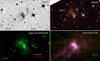 |
Fig. 1 Digital Sky Survey (DSS) R (top left), 2MASS composite image using the J, H, and Ks filters (top right), Spfeer/GLIMPSE360 4.5 μm (Sewiło et al. 2019; bottom left), and Herschel/Hi-GAL composite image at 70, 160, and 250 μm (Elia et al. 2013; bottom right) of the Gy 3–7 cluster. Circles in the top panels show the positions of YSO candidates from Tapia et al. (1997). Yellow diamond and red cross in the bottom-left panel show the position of the H2O maser (Urquhart et al. 2011) and the IRAS source at the south-west side (IRAS 07069–1045), respectively. The blue “×” symbols in the bottom right panel show the positions of dense cores as traced by the H2 column density (Elia et al. 2013). Dense core in the west corresponds to IRAS 07069-1045. |
Catalog of lines observed with FIFI-LS toward Gy 3–7.
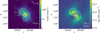 |
Fig. 2 Distribution of dust continuum emission toward Gy 3–7. Left: continuum map of Gy 3–7 at 70 μm observed with Herschel/PACS. Red “+” and blue “×” symbols refer to the 70 μm continuum peaks, adopted as the positions for the dense cores A and B in the subsequent analysis. Circles show the positions of HIGALBM224.6079–1.0065 and HIGALBM224.6128–1.0013 cores from the Herschel/Hi-GAL catalog (Elia et al. 2021). Right: map of the H2 column density (NH2). Black circles with the beam size of 20″ indicate the extract regions of the SOFIA FIFI-LS spectra toward the two dense cores A and B (see more in Sect. 3.1). White contours in each map show the continuum at 70 μm, with contour levels at 5, 10, 40, 80, 400, and 800 mJy arcsec−2. |
2.2 Herschel/PACS
We used the Herschel/PACS 70 μm continuum map to verify the positions of the dense cores in Gy 3–7 listed in the Herschel/Hi-GAL compact source catalogue4 (Elia et al. 2021). Figure 2 shows the 70 μm continuum map and the H2 column density, N(H2), map obtained using the ppmap tool with the Herschel/Hi-GAL survey (Marsh et al. 2017). Overall, there is a good agreement between the catalog positions and the peaks in the continuum at 70 μm and N(H2). In the subsequent analysis, we adopt the coordinates of the 70 μm peaks as the dense core coordinates. We refer to the core at (RA, Dec) = (7h09m20s.4, −10°50′28′.′/4) as A and to that at (7h09m21s.9, −10°50′35″) as B; they correspond to the Herschel/Hi-GAL catalog sources HIGALBM224.6079−1.0065 and HIGALBM224.6128–1.0013, respectively (Elia et al. 2021).
2.3 RT4
We conducted a survey at 22 GHz using the Toruń 32-m radio telescope (RT4) toward the entire CMa–l224 region. The full-beam width at half maximum of the antenna at 22 GHz is ~ 106″, with a pointing error of ≲12″ (Lew 2018).
Two series of observations were performed from 2019 April to 2020 January and from 2020 January to May 2020 in which a total of 205 positions were observed. We used the correlator with 2 × 4096 channels and 8 MHz bandwidth operating in the frequency-switching mode, which provided a local standard of rest velocity coverage from −11.9 to 41.9 km s−1. The spectral resolution of the observations is 0.03 km s−1. The observations were calibrated by the chopper wheel method and corrected for the gain elevation effect. The system temperature varied from −120 K during winter to ~200 K in summer. Overall, the 3σ detection limit was between ~3.8 and ~7.5 Jy per 0.03 km s−1 channel. The telescope pointing was checked every ~2 h by observing a nearby bright, point source. We successfully detected a variable water maser emission at (RA, Dec) = (7h09m21s.05, −10°50′05″.4), in direct vicinity of Gy 3–7, and at (RA, Dec) = (7h09m22s.66, −10°30′4y″.6), associated with IRAS 07069-1026 (see Appendix A).
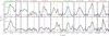 |
Fig. 3 SOFIA FIFI-LS continuum-subtracted spectra toward the two dense cores in Gy 3–7: HIGALBM224.6079–1.0065 (source “A”) and HIGALBM224.6128–1.0013 (source “B”). The emission is extracted within a beam size of 20″ indicated by black circles in the right panel of Fig. 2. Vertical lines show the laboratory wavelengths of the detected lines. Spectra of the [OI] line at 63 μm are multiplied by a factor of 0.2 and those of the CO 14–13 line by a factor of 0.6 to better illustrate the line detections. |
3 Results
Near-IR images of Gy 3–7 reveal an extended nebulosity associated with the two Hi-GAL dense cores and several YSO candidates (see Fig. 1). Spatially-resolved FIR line emission data obtained with FIFI-LS allows us to study key gas cooling lines at ~10 000 au scales and identify regions where processes responsible for the gas heating are at play.
3.1 Line detections
Figure 3 shows the FIR line emission toward the two Hi-GAL dense cores in Gy 3–7 (see Sect. 2.2; for the full list of targeted lines see Table 1). All lines are spectrally-unresolved with FIFI-LS and can be represented by single Gaussian profiles (Sect. 2.1).
The spectra show strong line emission in the [O I] lines at 63 μm and 145 μm, as well as in the high-J CO lines: the CO 14-13 line at 186.0 μm, the CO 16-15 line at 162.8 μm, and the CO 17-16 line at 152.3 μm. Core A shows also a detection of the CO 22-21 line at 118.6 μm (Eu of ~1400 K) and a tentative detection of CO 30-29 line at 87.2 μm (Eu of ~2600 K). The CO 31-30 line at 84.41 μm is blended with the OH line at 84.42 μm, and due to the lack of baseline covering the OH 84.6 μm line from the doublet, its emission cannot be quantified. The OH doublet at ~79.2 μm seems to be tentatively detected toward both cores, but is severely affected by the rise of the baseline on its left side and its flux cannot be properly measured (Appendix B). The OH doublet at 163.12 and 163.18 μm, located next to the CO 16–15 line, is not detected in neither of the two cores.
The [O I] line at 63.18 μm sits on the edge of a telluric water feature and the low transmission at λ ≳ 63.24 μm increases the noise on the continuum. Since the transmission at the spectral line location is well known and the S/N is very high, there is no relevant effect on the uncertainty of the line flux. Possible self-absorption of this [OI] line cannot be identified at the spectral resolution of FIFI-LS. The higher-resolution spectra collected toward other YSOs using the German REceiver for Astronomy at Terahertz Frequencies (GREAT; Risacher et al. 2018) show that self-absorption could decrease the integrated emission of the line by a factor of 2–3 (Leurini et al. 2015; Mookerjea et al. 2021).
Similarly, self-absorption in the [CII] line at 157.7 μm might affect the FIFI-LS spectra. Strong self-absorption unresolved by FIFI-LS may result in a non-detection of this line toward core A. In contrast, the line is clearly detected toward core-B. Decreases of the flux of [C ii] line due to self-absorption as high as a factor of 20 have been estimated toward photodissociation regions (Guevara et al. 2020).
In summary, FIFI-LS spectra provide detections of key FIR cooling lines toward two dense cores in Gy 3–7: the high-J CO, [O I], and [C II]. Due to the atmospheric absorption, the H2O emission could not be targeted; the OH emission suffers from line blending and poor baselines. In Sect. 3.2, we show the distribution of line emission in various species toward the entire cluster.
3.2 Spatial extent of FIR line emission
The FIR range contains several important diagnostic lines, which provide information about the physical conditions and processes that strongly contribute to the gas cooling (Goldsmith & Langer 1978; Kaufman & Neufeld 1996). The analysis of spatial extent of various FIR species pinpoints the presence of shocks and/or UV radiation associated with star formation.
Figures 4 and 5 show the spatial extent of the FIR lines detected toward Gy 3–7 (Sect. 3.1). The line emission is compared to the FIR dust continuum emission at 70 or 160 μm from Herschel/PACS (Fig. 4) and the 4.5 μm continuum tracing warmer dust from Spitzer/IRAC (Fig. 5). Bright rotationally excited H2 emission associated with shocks might also contribute to the flux in the 4.5 μm IRAC band (Cyganowski et al. 2008, 2011). Appendix B shows additional maps of Gy 3–7 for lines from various species.
The high-J CO emission distribution is elongated in the same direction as the IR continuum, but its peaks are offset from the continuum peaks at wavelengths similar to those of the respective CO lines. A similar pattern of emission is also seen for the [O I] 63 μm and 145 μm lines; yet, the peak of the [O I] lines are almost co-spatial with the core positions, which is not the case for the CO lines. Nevertheless, both the CO and the [OI] extend beyond the core positions along the E–W direction. Such elongated high-J CO morphologies have been commonly interpreted as arising in shocked outflows from LM and IM protostars (Goicoechea et al. 2012; He et al. 2012; Kristensen et al. 2012, 2017b; Karska et al. 2013; Matuszak et al. 2015; Green et al. 2016; Tobin et al. 2016). Similarly, extended [O I] emission has been associated with embedded, atomic outflows (Karska et al. 2013; Nisini et al. 2015), as recently confirmed by detections of broad line wings in the 63 μm line with SOFIA/GREAT (Leurini et al. 2015; Kristensen et al. 2017a; Yang et al. 2022a). Thus, the high-J CO and [O I] emission toward Gy 3–7 might also arise from outflows, where shocks and UV radiation both contribute to gas cooling (see Sect. 5).
The [C II] emission also follows the pattern of the continuum emission, but its two emission peaks are offset by ~11″ in different directions from the corresponding [O I] 63 μm peaks. These differences are illustrated further in Fig. 6, in which emission in various species is directly compared. Clearly, the [C II] emission traces different regions of Gy 3–7 than the high-J CO and [O I] lines, which is at least partly due to its lower critical density, ncrit ~(3.7–4.5) × 103 cm−3 for Tkin of 300–100 K (assuming collisions with H2, Wiesenfeld & Goldsmith 2014). As a result, [C II] is excited in lower density regions and likely exposed to external UV radiation creating a photodissociation region (Hollenbach & Tielens 1997). To some extent, the pattern of [C II] emission might be also affected by self-absorption, which is spectrally-unresolved in the FIFI-LS data (Sect. 3.1).
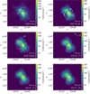 |
Fig. 4 FIFI-LS contour maps of the [O I] lines at 63.2 and 145.5 μm, the [CII] line at 157.7 μm, the CO lines with Jup = 14, 16, 17 at 186, 163, and 153 μm respectively (white contours) on top of the continuum emission at 160 μm (at 70 μm for the [OI] line at 63.2 μm) from Herschel/PACS. The white contours show line emission at 25%, 50%, 75%, and 95% of the corresponding line emission peak. The “+” and “×” signs show the positions of the dense cores A and B. |
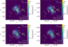 |
Fig. 5 FIFI-LS contour maps of the [O I] lines at 63.2 and 145.5 μm, the [CII] line at 157.7 μm, and the CO 14-13 line at 186 μm (white contours) on top of the continuum emission at 4.5 μm from Spitzer/IRAC. The contours show line emission at 25%, 50%, 75%, and 95% of the corresponding line emission peak. The “+” and “×” signs show the positions of the dense cores A and B, respectively. The orange squares show the positions of two YSO candidates with envelopes, and the yellow circles show the positions of the remaining YSOs (Sect. 4.5). |
4 Analysis
The high-J CO emission allows us to measure the CO rotational temperature of the warm molecular gas and to estimate the total line cooling by the FIR CO lines. The mapping capabilities of FIFI-LS provide information about the spatial distribution of the temperature and gas cooling across the entire clump.
4.1 CO rotational temperatures
We used Boltzmann (or rotational) diagrams to calculate the CO rotational temperature toward the two dense cores in Gy 3–7 as a proxy of gas kinetic temperature. Assuming that all these lines are optically thin and thermalized, their upper level column densities, Nu, are estimated using Eq. (1) following Goldsmith & Langer (1999):
 (1)
(1)
where gu is the degeneracy of the upper level, Q(Trot) is the rotational partition function at a temperature, Trot, Ntot is the total column density, and kB is the Boltzmann constant (see Table 1).
Due to the low spatial resolution of FIFI-LS, the emitting region of the highly-excited gas is unresolved and thus we calculate instead the number of emitting molecules, 𝒩u, for each transition (see e.g., Herczeg et al. 2012; Karska et al. 2013):
 (2)
(2)
where Fλ is the flux of the line at wavelength λ, d is the distance to Gy 3–7, A is the Einstein coefficient, c is the speed of light, and h is the Planck’s constant. Consequently, the total number of emitting molecules 𝒩tot is derived instead of the Ntot from Eq. (1). To measure Trot over the same physical scales, we convolved the CO emission maps down to the lowest spatial resolution corresponding to CO 14–13 observation (18.3″, see Table 1) and resampled the maps to the same pixel size.
The flux of CO lines toward cores A and B was calculated within a beam of 20″ (see Table B.1). We performed a linear fit on the rotational diagram using the curve_fit function in Python (y = ax + b). The Trot and 𝒩tot values are derived from the slope a and y-intercept b of the fit (Eq. (1)).
Figure 7 shows the CO Boltzmann diagrams toward the two cores in Gy 3–7. We obtain rotational temperatures of 305 ± 85 K and 155 ± 20 K toward dense cores A and B, respectively, using CO lines with Jup of 14–22 (see Table 2). The same transitions have been associated with the “warm” component detected on CO diagrams toward protostars in the inner Galaxy and corresponding to the widely found Trot of 300 K (Karska et al. 2013; Manoj et al. 2013; Green et al. 2013). The CO 30–29 and CO 31-30 data at 87.2 and 84.4 μm, respectively, indicate the presence of the “hot” component toward core A (Karska et al. 2013). However, the 84.4 μm line is blended with OH, which clearly affects the CO line flux (see Fig. 3). Consequently, we are not able to constrain the “hot” component using only the CO 30-29 line.
The spatial distribution of the “warm” component’s CO rotational temperature toward the entire Gy 3–7 clump is shown in the left panel of Fig. 8. Here, we calculate Trot using the three lowest transitions (Jup of 14–17), which are detected in a large part of the map, except for the map edges where even CO 17–16 is not detected (Fig. 4). The resulting Trot values range from 105 to 230 K across the map, with a median value of 170(15) ± 30 K5. The CO rotational temperatures are the highest in the vicinity of the CO 17–16 emission peaks, which are offset by ~17″ from core A to the west (Fig. 4). The morphology of the Trot distribution suggests the origin of high-J CO in a bipolar outflow driven by core A. Significantly lower CO temperatures, ≲150 K, are measured in the surroundings of core B, without a clear outflow signature from this object. The temperatures around 200 K at the eastern edge of the map are likely caused by higher gas densities in this region, rather than higher gas kinetic temperatures.
The spatial distribution of dust temperatures Tdust toward Gy 3–7, adopted from the Herschel/Hi-GAh survey, is also shown in the right panel of Fig. 8. The morphology of regions with elevated temperatures is similar to the extent of N(H2), and shows two peaks at 27 and 21 K toward core A and B, respectively. The pattern differs significantly from the distribution of warm, ~300 K gas, traced by CO lines, favoring the origin of the CO emission in a bipolar outflow driven by core A. Nevertheless, the lowest-J CO transitions observed with FIFI-LS might partly trace the extended continuum emission, for instance, on the eastern part of Gy 3–7. We discuss this issue further in Sect. 5.1.
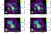 |
Fig. 6 Integrated intensity maps of selected pairs of FIR lines from FIFI-LS with the top line shown in colors, and the bottom line in white contours. The contour levels are 25%, 50%, 75%, and 95% of the corresponding line emission peak. The “+” and “×” signs show the positions of the dense cores A and B, respectively. The spaxel size in the emission map of the [O I] line at 63 μm is 6″ × 6″ (blue channel) and in the map of other lines (CO 14-13, [OI] at 145 μm, and [CII] at 157.7 μm) is 12″ × 12″ (red channel). Gray circles show the beam size for each color map. |
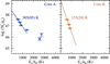 |
Fig. 7 CO rotational diagrams toward core A (left, in blue) and B (right, in orange). Circles refer to values based on line detections and the triangle shows the measurement using the upper limit of the CO 31-30 line, which is blended with OH. Solid lines show fits using transitions belonging to the “warm” gas component; the CO 30–29 line at 87.19 μm is therefore not included. The CO rotational temperature Trot derived from the rotational diagram is labeled in each panel and the value in parenthesis indicates its uncertainty. |
CO rotational temperature, the number of emitting molecules, and total line luminosities of CO and [O I] lines toward dense cores in Gy 3–7 and IM YSOs from Matuszak et al. (2015).
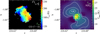 |
Fig. 8 Gas and dust temperatures toward Gy 3–7. Left: CO rotational temperature map obtained using Boltzmann diagrams. White contour map shows the CO 17–16 emission at 25%, 50%, 75%, and 95% of the emission peak. Right: H2 column density contour map overlaid on the dust temperature map derived from the ppmap tool with the Herschel/Hi-GAL survey (Marsh et al. 2017). Contour levels of the N(H2) are at (5, 10, 30, 50, 55) × 1021 cm−2. |
4.2 FIR line cooling
The FIR line cooling budget in LM protostars is sensitive to a source’s evolutionary stage and Lbol, and its contributions provide important information on the shock origin of the FIR emission (Karska et al. 2013, 2018). Here, we quantify the luminosity of the FIR CO and [O I] lines toward the two cores in Gy 3–7 and a sample of IM protostars observed with Herschel/PACS (Matuszak et al. 2015).
4.2.1 Calculation procedure
We calculated the line cooling following procedures developed for Herschel/PACS observations in the same wavelength range (Karska et al. 2018). Briefly, we determined the line luminosity of CO lines in the “warm” component, LCO(warm), from the sum of the individual line fluxes with Jup from 14 to 24, corresponding to Eu/kB = 580–1800 K. Since not all CO transitions are observed, we use linear fits from the Boltzmann diagram to the “warm” component to recover the fluxes of the transitions not covered by FIFI-LS or PACS observations. The flux uncertainties of those transitions were propagated from the parameters of the linear fit and their uncertainty. The same procedure could be applied to the “hot” component toward Gy 3–7 cores due to the lack of data on a sufficient number of high-J CO transitions. As a result, we did not calculate the total FIR CO cooling, that is, we did not account for transitions with Eu>1800 K. The advantage of this approach is that we avoid significant source-to-source variations in LCO(hot), which is reflected by the broad range of rotational temperatures measured using the highest-J CO lines (see Fig. 6 in Karska et al. 2018). The total line luminosity of [O I], L[O I], is calculated by the addition of the fluxes of the [O I] 63 and 145 μm lines. Table 2 shows the FIR line luminosities obtained for Gy 3–7, as well as those for six IM YSOs from Matuszak et al. (2015).
Figure 9 shows the spatial distribution of the FIR line luminosity of CO and [O I] toward Gy 3–7. Most of the CO luminosity orginates in a region west of core A, suggesting an outflow origin (see also Sect. 3.2). A similar region is characterized also by a high [O I] luminosity, which typically follows the pattern of high-J CO emission around LM protostars (Karska et al. 2013; Nisini et al. 2015; van Dishoeck et al. 2021). Additionally, a high [O I] luminosity is measured to the east from core B, toward the direction of the [C II] peak (see Figs. 5 and 6). The lack of enhancement of CO line luminosity in this region could suggest an origin of the [O I] emission in the PDR. We explore this scenario further in Sect. 4.3.
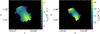 |
Fig. 9 Spatial extent of FIR line luminosities of CO (left) and [O I] (right) toward Gy 3–7. The calculation procedure is described in Sect. 4.2. |
4.2.2 Flux correlations
We compare the FIR line emission in Gy 3–7 with the data based on Herschel/PACS measurements toward LM Class 0 and Class I (Karska et al. 2018), IM (Matuszak et al. 2015), and HM YSOs (Karska et al. 2014a). CO luminosities are consistently calculated for the “warm” component on Boltzmann diagrams. The correlations between luminosities of the two [O I] lines, as well as the [O I] and CO lines are shown in Fig. 10.
A strong power-law correlation is found between the [O I] line luminosities for all low- and intermediate-mass sources including the two cores in Gy 3–7 (the Pearson coefficient of the correlation is r = 0.996, which corresponds to a significance of 8.2σ). The observed ratios of the [O I] 63 μm/145 μm lines span a range from 4 to 38 with a median value of ~12. These results are quantitatively similar to those shown in Fig. 11 of Karska et al. (2013) for a sub-sample of 18 LM YSOs.
The HM YSOs follow a similar trend, however, several sources show a flux deficit in the [O I] 63 μm line, which is likely caused by line-of-sight contamination and optical depth effects (see, e.g., Liseau et al. 1992; Leurini et al. 2015). A power-law fit to the sample including HM YSOs shows a shallower slope (b = 0.91 versus b = 0.99, when only LM and IM YSOs are considered). The correlation strength is comparable to the one for LM and IM sources alone, with a Pearson coefficient of 0.991 corresponding to 8.5σ.
The CO line luminosity in the “warm” component shows a strong correlation with the 145 μm [O I] line luminosity. A power-law fit to the entire sample returns a slope of b ~0.93 and the Pearson coefficient of 0.971, corresponding to 8.2σ (Fig. 10). Clearly, the line luminosity of the [O I] 145 μm line shows a smaller scatter for the HM YSOs with respect to the 63 μm line. In case of LM YSOs, a significant scatter in the ratio of CO and [O I] line luminosities is likely linked to their different evolutionary stages. The ratio of CO line luminosity over Lbol is ~2.3 larger for Class 0 than Class I sources, whereas the [O I] luminosities are similar for both groups (Karska et al. 2018). Thus, the molecular-to-atomic line cooling is expected to be higher in Class 0 objects. Indeed, the linear fit using only Class 0 sources results in a shallower slope, but do not affect the general conclusions.
In summary, we find a strong correlation between the line luminosities of the [O I] and CO lines for YSOs in a broad mass range, consistent with previous results for LM YSOs (Karska et al. 2013). Combined with the similar spatial extent of the [O I] and CO lines (Sect. 3.2), the correlations suggest a similar physical origin of the two species.
4.3 Properties of a possible photodissociation region
Assuming that the [O I] and [C II] lines predominately arise from a photodissociation region (PDR), the UV field strengths, G0, and hydrogen nucleus number densities, nH, across Gy 3–7 can be obtained from their ratios. These assumptions might be justified in case of the eastern part of Gy 3–7 with relatively weak CO line luminosities (see Sect. 4.2). On the contrary, the [O I] line luminosity in the surrounding of core A closely follows the high-J CO emission associated with outflow shocks.
We determined the physical properties of the PDR using the PDR Toolbox 2.1.16 (Pound & Wolflre 2011) based on the PDR models provided by Kaufman et al. (2006). We used three line ratios involving the [O I] lines at 63.2 μm and 145.5 μm, and [CII] line at 157.7 μm, and ran the code at each spaxel of the FIFI-LS maps. We obtained gas densities of 104–105 cm−3 and UV field strengths of the order of 103–106 times the average interstellar UV radiation field (Habing 1968). These physical conditions are typical for dense, star-forming clumps associated with HM YSOs (Ossenkopf et al. 2010; Benz et al. 2016; Mirocha et al. 2021). However, given that Gy 3–7 is associated with IM YSOs (see Sect. 4.5), UV radiation fields of 103 or higher are unlikely (e.g., Karska et al. 2018).
The similar spatial extent of the [OI] and high-J CO emission (Sect. 3.2) and the strong line luminosity correlation between the two species (Sect. 4.2) favor the origin of the bulk of [O I] in the outflow shocks rather than in the photodissociation region. We consider this scenario in Sect. 4.4.
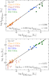 |
Fig. 10 Correlations between luminosities of FIR CO and [O I] lines. Top: correlation between the luminosities of the 63 and 145 μm [O I] lines at from LM to HM YSOs. Cores A and B in Gy 3–7 are marked as grey diamonds, Class 0 and Class I YSOs as orange "×" signs and red circles (Karska et al. 2018), respectively, IM YSOs as blue circles (Matuszak et al. 2015), and HM YSOs as green squares, respectively (Karska et al. 2014a). Black solid line is the linear fit to all sources except for the HM YSOs, showing a strong correlation between the two [O I] line luminosities. Bottom: correlation between luminosities of the CO lines and the [O I] line at 145 μm. Black solid line shows the linear fit to all sources, including the HM YSOs. |
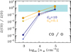 |
Fig. 11 Ratio of the CO and [O I] luminosities as a function of preshock density for UV irradiated C–shock models and observations of Gy 3-7 cores and IM YSOs from Matuszak et al. (2015; light blue box). All models correspond to UV fields parameterized by G0 of 10 (in blue) and 0.1 (in orange). Solid lines connect models with shock velocities vs of 20 km s−1, and dashed lines – the models with vs of 10 km s−1. |
4.4 Comparisons with UV-irradiated shocks
Bright FIR emission detected toward LM YSOs has been interpreted in the context of continuous (C–type) shocks irradiated by UV photons (Karska et al. 2014b; Kristensen et al. 2017b). Figure 11 shows a comparison of the FIR observations toward IM YSOs, including two cores in Gy 3–7, and the UV-irradiated shock models from Melnick & Kaufman (2015) and Karska et al. (2018).
Predictions of shock models were previously calculated for high-J CO lines covered by Herschel/PACS. Here, we show the predictions for UV field strengths, G0, of 0.1 and 10, and shock velocities of 10 and 20 km s−1 (see also Fig. 14 in Karska et al. 2018). For the sake of comparison, we calculated the total FIR line luminosity of CO using the transitions in the “warm” component (Sect. 4.2.1), as well as high-J CO lines, both for Gy 3–7 and for IM YSOs (Matuszak et al. 2015). The [O I] line luminosity is calculated from the sum of the two fine-structure [O I] lines.
The models show a good match with observations for preshock H2 number densities of 105 cm−3 and the entire range of the considered UV radiation field strengths. For shock velocities, vs, of 20 km s−1, a possible match is also found for pre-shock densities of 104 cm−3 and G0 of 0.1. The compression factor >10 is expected in C–type shocks (Karska et al. 2013), so the gas densities are of the order of 105−106 cm−3, in agreement with those of LM YSOs (e.g., Kristensen et al. 2012; Mottram et al. 2017).
Due to the lack of H2O observations from FIFI-LS and non-detections of OH, we are limited to comparisons between CO and [O I] lines. Some of the [O I] emission might arise in the PDR (Sect. 4.3), which would increase the observed line luminosity ratio; however, the strong correlation of [O I] and high-J CO tracing outflow shocks does not support this scenario.
Best-fit models of SED using the Robitaille (2017) classification.
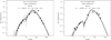 |
Fig. 12 SEDs of YSOs in Gy 3-7 well-fitted with Robitaille (2017) models with envelopes. The best fit model is indicated with the black solid line and gray lines show the YSO models with χ2 between |


4.5 Spectral energy distribution analysis
We investigate the physical properties of 15 individual YSO candidates from Tapia et al. (1997) and Sewiło et al. (2019) in Gy 3–7 to understand their possible impact on the FIR and submillimeter line emission. Spectral energy distribution (SED) models of YSOs from Robitaille (2017) are fitted to the multi-wavelength photometry of YSOs using a dedicated fitting tool (Robitaille et al. 2007). Multi-wavelength photometry spanning from near- to mid-IR range of YSO candidates in the IRAS field is presented in Appendix C.
We followed the procedures described in detail in Karska et al. (2022). We used 18 sets of model SEDs including various physical components of a YSO: star, disc, in-falling envelope, bipolar cavities, and an ambient medium (Robitaille 2017). We used the PARSEC evolutionary tracks produced by the revised Padova code (Bressan et al. 2012; Chen et al. 2014, 2015; Tang et al. 2014) to quantify the results of SED model fitting. Models producing YSO parameters outside of the PARSEC pre-main sequence (PMS) tracks were excluded. YSOs with models in line with the PARSEC tracks are illustrated on the Hertzsprung-Russell diagram in Appendix C. For those YSOs, we calculate the stellar luminosity from the Stefan–Boltzmann law, using the stellar radius and effective temperature from the SED fitting. The masses and ages are determined from the closest PMS track; however, we only provide the stellar masses and ages that are consistent with the SED fitting results (i.e., the evolutionary stage) and YSO lifetimes from Dunham et al. (2015), respectively (see Sect. 3.7 in Karska et al. 2022).
Table 3 shows the best-fit SED models for 12 YSOs in Gy 3–7. The SEDs of two sources require an envelope contribution which is typical for deeply-embedded Class 0/I YSOs (see Fig. 12), while six sources are successfully modeled with a passive disk and four are normal stars (see Appendix C). The resulting physical parameters determined from SED models are shown in Table 4.
The two YSOs with envelopes, No. 10 and 12 in Table 4, are located in the center of Gy 3–7 (see Figs. 1 and 5), and their strong IR excess has already been noted by Tapia et al. (1997). The Class 0 YSO is co-spatial with the IRAS source and the dense core A (Elia et al. 2021), and might be the source of the outflow responsible for the FIR emission. Both objects are in the IM regime based on their luminosities obtained from SEDs. The four objects that are modeled as stars with foreground extinction have photometry only from 1 to 5 μm. In this range, it is difficult to distinguish between stars with foreground extinction and stars with disks, so we do not rule out the latter explanation.
5 Discussion
Far-IR observations from FIFI-LS confirm the status of Gy 3–7 as a deeply-embedded cluster, as originally proposed by Tapia et al. (1997). Here, we discuss the likely origin of FIR emission in Gy 3–7 and we search for any effects coming from metallicity by comparison with YSOs from the inner Galaxy.
Physical parameters for a subset of YSO candidates with at least five photometric data points.
5.1 Origin of FIR emission in Gy 3–7
A strong correlation of high-J CO and [OI] luminosities and their spatial extent in Gy 3–7 provides a strong support toward the common origin of the two species. The modeling of envelopes of HM YSOs showed that emission from shocks is necessary to reproduce line fluxes of high-J CO lines (Karska et al. 2014a). The same is certainly the case for LM and IM YSOs as well, which are characterized by lower envelope densities and temperatures. On the other hand, the [O I] emission could be associated with a photodissociation region (Kaufman & Neufeld 1996; Hollenbach & Tielens 1997) or outflow shocks (Karska et al. 2013; Nisini et al. 2015). Recent velocity-resolved profiles of the [O I] line at 63 μm with SOFIA/GREAT support the later scenario for LM YSOs, which does not suffer from strong self-absorption (Kristensen et al. 2017a; Yang et al. 2022a). Therefore, we assume that the entire high-J CO and [O I] emission originates from outflow shocks. As shown in Sect. 4.4, the line luminosity ratio of CO and [O I] is consistent with C-type shocks irradiated by UV fields of 0.1–10 times the average interstellar radiation field and pre-shock densities of 104–105 cm−3 (see also Melnick & Kaufman 2015; Karska et al. 2018). The detection of variable H2O maser further confirms the outflow activity in the region (Furuya et al. 2003). We provide details in Appendix A.
The physical conditions in Gy 3–7 are also constrained by CO rotational temperatures, which provide a good proxy of gas kinetic temperatures (Karska et al. 2013; van Dishoeck et al. 2021). The high-J transitions are likely optically thin and ther-malized at gas densities >105 cm−3 that are routinely measured for LM and IM YSOs (e.g., Kristensen et al. 2012; Mottram et al. 2017). The top panel in Fig. 13 shows that Trot, CO associated with the two dense cores in Gy 3−7 is either fully consistent (core A) or at the low-end of other IM YSOs (core B), for which the median value from the literature is 320(33) ± 35 K (Matuszak et al. 2015). Similar rotational temperatures have been measured for LM and HM YSOs (Karska et al. 2013, 2014a, 2018; Green et al. 2013, 2016; Manoj et al. 2013; Yang et al. 2018), with average values of 328(33) ± 63 K (Karska et al. 2018) and 300(23) ± 60 K (Karska et al. 2014a), respectively.
Some differences between the dense core B in Gy 3–7 and the other YSOs studied in the literature might result from a smaller number of transitions probed by FIFI-LS. The curvature seen in the rotational diagrams causes the rotational temperature to be underestimated if high-J CO transitions are not observed. Therefore, we re-calculated all literature measurements of Trot for IM and HM YSOs using the same or similar transitions as obtained for Gy 3–7 (Table 2 and Appendix D). As expected, CO rotational temperatures for IM and HM YSOs are now lower than reported in the literature and consistent even with core B (see bottom panel of Fig. 13).
5.2 Possible impact of metallicity on FIR line emission in the outer Galaxy
Far-IR observations of HM YSOs in the low-metallicity environments of the SMC and LMC show a lower fraction of molecular-to-atomic emission with respect to Galactic YSOs (Oliveira et al. 2019). Here, we investigate the impact of bolo-metric luminosity, Lbol, and source Galactocentric radius, RGC, on the ratio of CO and [O I] line luminosity.
Figure 14 shows the molecular-to-atomic ratio toward Gy 3–7 cores and other Galactic IM and HM YSOs as a function of Lbol. The values of Lbol for the two cores in Gy 3–7 are adopted from Elia et al. (2021), and are equal to 75.9 and 324.2 L⊙, respectively. The correlation is characterized by a Pearson coefficient of 0.19, corresponding to 1.6σ. Since the number of LM YSOs exceeds by far the number of IM and HM sources, we also search for trends in the binned datasets. We bin sources in equal intervals of logLbol=1, and adopt a 1 σ variance of the distribution as the uncertainty inside the bin. As a result, we confirm a weak correlation between the ratio of line luminosity and Lbol (r ~0.59, corresponding to 1.5σ). Thus, our large sample of YSOs starts to reveal a relationship between the mass of YSOs and the fraction of molecular-to-atomic cooling. This has not been possible with a sample of 18 LM YSOs and 10 HM YSOs analyzed in Karska et al. (2014a), where a ratio of ~4 was reported for YSOs in the entire mass regime. We note, however, that the Herschel/PACS measurements from the literature benefited from additional detections of H2O and OH, which were included in the molecular FIR cooling.
Figure 15 shows the molecular-to-atomic ratio as a function of Galactocentric radius. In addition, Fig. 16 shows the same ratio as a function of metallicity, Z, estimated assuming elemental abundance gradients derived from H II regions (Balser et al. 2011). Appendix D provides heliocentric distances, Galactocentric radii, and metallicities of Galactic sources, as well the measurements of CO and [O I] for YSOs in both the Milky Way and the Magellanic Clouds.
The molecular-to-atomic ratio decreases very weakly with the Galactocentric radius (Fig. 15) but the Pearson coefficient is too small to confirm the correlation (r = 0.08, corresponding to 0.7σ). Additional observations of YSOs in the outer Galaxy would be necessary to constrain the molecular-to-atomic ratio, in particular, in the gap between 10 and 12 kpc. Due to the lack of such observations, we searched for trends as a function of metallicity by including YSOs in the Magellanic Clouds (Fig. 16). We note, however, that the [O I] line at 145 μm was not observed toward sources in the Magellanic Clouds, and the ratio of the two [O I] lines calculated for LM YSOs from Karska et al. (2018) was adopted to estimate its fluxes (Oliveira et al. 2019). As seen in Fig. 10, this ratio may differ for HM YSOs due to self-absorption or optical depth effects in the [O I] 63 μm line. Additionally, the total CO luminosity of YSOs in the SMC and LMC was estimated using the detections in SPIRE and the conversion factor from Yang et al. (2018), also based on LM YSOs.
In conclusion, Gy 3–7 follows closely the correlations set by YSOs observed in the Milky Way and the Magellanic Clouds. The ratio of molecular-to-atomic line emission is dominated by source bolometric luminosities, and only a very weak decreasing trend with the Galactocentric radius was detected.
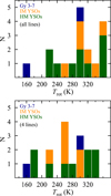 |
Fig. 13 CO rotational temperatures for dense cores in Gy 3–7 and intermediate- and high-mass YSOs from the literature (Karska et al. 2014a; Matuszak et al. 2015). Top: straightforward comparison with the literature values. Bottom: Comparison accounting for the number of observed CO lines considered in the rotational diagrams. |
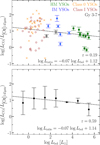 |
Fig. 14 Correlations between the ratio of CO and [O I] line luminosities and bolometric luminosity of YSOs in the two cores in Gy 3–7 (gray diamonds), Class 0 and Class I YSOs (orange ‘×’ signs and red circles, respectively; Karska et al. 2018), IM YSOs (blue circles; Matuszak et al. 2015), and HM YSOs (green squares; Karska et al. 2014a). The bolometric luminosities for Gy 3–7 cores are adopted from Elia et al. (2021). The top panel shows a power-law fit to all individual data points, and the bottom panel shows the fit to the data bins (both shown as black dashed line). |
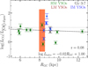 |
Fig. 15 Ratio of molecular to atomic line luminosities as a function of the Galactocentric radius. The light coral box indicates the range of the line luminosity ratio and the Galactocentric radius for LM YSOs in the nearby clouds, which are excluded from the power-law fit to the remaining YSOs (dashed black line). Gray dotted horizontal line indicates where the molecular luminosity is equal to the atomic luminosity. |
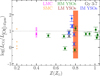 |
Fig. 16 Ratio of molecular to atomic line luminosities as a function of metallicity, Z. HM YSOs in the SMC and LMC are shown with cross and “×” symbols in orange and purple colors, respectively. The light coral box indicates the range of the line luminosity ratio and the metallicity for LM YSOs in the nearby clouds, which are excluded from the power-law fit to the remaining YSOs (dashed black line). The gray dotted horizontal line indicates where the molecular luminosity is equal to the atomic luminosity. |
6 Conclusions
We investigated the SOFIA/FIFI-LS maps of the CO transitions from J = 14-13 to J = 31-30, the [O I] lines at 63.2 μm and 145.5 μm, and the [C II] 158 μm line toward the outer Galaxy cluster Gy 3–7. Spatial information on the FIR emission enabled us to quantify such physical parameters as temperatures, densities, and UV radiation fields, as well as to associate them with identified YSOs. Our conclusions are as follows:
The CO J = 14-13 to J = 16-15 emission lines are detected in a significant part of Gy 3–7, where Herschel/PACS 160 μm continuum emission is also strong. Higher–J CO lines up to 31-30 are clearly detected only toward the dense core A.
The spatial extent of the [O I] emission at 63 and 145 μm is similar to that of CO 14-13 and the 70 and 160 μm continuum emission. The [C II] emission is also extended, but shows systematic shifts in the emission peaks away from the FIR continuum, tracing lower density gas.
The CO rotational diagrams show the warm components toward two cores with Trot of 305 and 155 K, and a range of Trot from ~105 to 230 K throughout the cluster, where only three high-J CO lines are unambiguously detected. Similar rotational temperatures have been detected toward IM and HM YSOs in the inner Milky Way calculated using the same or similar CO transitions.
A strong correlation of the CO and [O I] line luminosities and their similar spatial extent point at the common origin in the outflow shocks. The CO/[O I] line luminosity ratio of Gy 3–7 cores and other intermediate-mass YSOs is consistent with C-type shocks propagating at pre-shock densities of 104–105 cm−3 and UV fields of 0.1–10 times the average interstellar radiation field.
Physical parameters for 15 YSO candidates in the Gy 3–7 cluster are obtained from a YSO SED model fitting (Robitaille 2017). Two sources, corresponding to Hi-GAL dense cores from Elia et al. (2021), are well-fitted with YSO models including the envelope, confirming their early evolutionary stage (Class 0/I). The location of the Class 0 source at the center of Gy 3–7 cluster suggests that it might be the driving source of the outflow revealed by FIR emission.
The ratio of warm CO and [O I] at 145 μm line luminosities from protostellar envelopes shows a weak decreasing trend with the bolometric luminosity and Galactocentric radius. We do not identify any significant dependence of the line cooling in Gy 3–7 on metallicity.
High-resolution submillimeter observations would be necessary to unambiguously associate FIR emission from FIFI-LS with candidate YSOs and their outflows. Alternatively, the efficient imaging of Gy 3–7 with the Mid-Infrared Instrument on board James Webb Space Telescope in F560W and/or F770 W filters tracing H2 emission would unveil the details in the outflows (Yang et al. 2022b).
Acknowledgements
N.L., A.K., M.F., M.G., M.K., and K.K. acknowledge support from the First TEAM grant of the Foundation for Polish Science no. POIR.04.04.00-00-5D21/18-00 (PI: A. Karska). A.K. also acknowledges support from the Polish National Agency for Academic Exchange grant no. BPN/BEK/2021/1/00319/DEC/l. This article has been supported by the Polish National Science Center grant 2014/15/B/ST9/02111 and 2016/21/D/ST9/01098. The material is based upon work supported by NASA under award number 80GSFC21M0002 (MS). The research is supported by a research grant (19127) from VILLUM FONDEN (LEK). This work is based (in part) on observations made with the NASA/DLR Stratospheric Observatory for Infrared Astronomy (SOFIA). SOFIA is jointly operated by the Universities Space Research Association, Inc. (USRA), under NASA contract NNA17BF53C, and the Deutsches SOFIA Institut (DSI) under DLR contract 50 OK 2002 to the University of Stuttgart. The 32 m radio telescope is operated by the Institute of Astronomy, Nicolaus Copernicus University and supported by the Polish Ministry of Science and Higher Education SpUB grant.
Appendix A Water masers in CMa-l224
Appendix A.1 : Survey results
Water masers are important signposts of both low- and high-mass star formation; they are collisionally excited, tracing warm molecular gas behind shock waves in the environment of YSOs and Hii regions (e.g., Litvak 1969; Elitzur et al. 1989; Furuya et al. 2003; Ladeyschikov et al. 2022 and references therein). Figure A.1 shows the pointings of our 22 GHz water maser survey of the CMa-/224 star-forming region with the 32-m radio telescope in Torun (RT4; a half-power beam width, HPBW~106”, corresponding to ~0.5 pc at 1 kpc; see Sect. 2.3), overlaid on the CO 1-0 integrated intensity image from the Forgotten Quadrant Survey (FQS, Benedettini et al. 2020; HPBW-55” at 115 GHz). The RT4 water maser survey targeted the fields harboring YSO candidates identified by Sewiło et al. (2019). Out of 205 observed fields, (185, 18, 2) were observed in (2, 3, 6) epochs. Water masers were detected toward two fields, one centered on Gy 3-7 and the other on source IRAS 07069-1026 in the main filament in CMa-/224. The very low detection rate is likely the result of the low sensitivity of our observations and the variability of the maser emission (see Sect. 2.3).
The detection of the water maser toward IRAS 07069–1026 constitutes the first maser detection toward this source, while the detection toward Gy 3–7 has previously been reported in the literature. Urquhart et al. (2011) detected the 22 GHz water maser emission toward Gy 3–7 (their source G224.6075-01.0063) with the 100-m Green Bank Telescope (GBT; HPBW~30″). Water masers were detected toward two other locations in CMa–l224 by Valdettaro et al. (2001) with the Medicina 32-m radio telescope (a similar angular resolution as for RT4), toward IRAS 07077–1026 and IRAS 07054–1039 (see Figure A.1).
The water maser spectra for Gy 3–7 and IRAS 07069-1026 for all epochs of the RT4 observations are shown in Figure A.2 and Figure A.3, respectively. Gy 3–7 was observed with RT4 six times over five months with the time interval between subsequent epochs ranging from 2 days to over two months (see Table A.1 for observing dates). The water maser emission was detected in all epochs. IRAS 07069–1026 was observed in two epochs separated by about six months (see Table A.1). The water maser emission toward IRAS 07069-1026 was only detected in the second epoch, illustrating a high variability of the water maser phenomenon. The RT4 spectra of Gy 3–7 also show clear evidence for a variable nature of the maser emission in this region. Both the peak flux density and central velocity of the maser spots varied significantly between April 2019 and May 2020, covering the flux density and velocity ranges of 4.4–117.2 Jy and 1.8–3.9 km s−1, respectively.
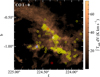 |
Fig. A.1 CO 1 – 0 integrated intensity map of CMa-l224. Yellow circles show all RT4 pointings, while white circles indicate those with the 22 GHz water maser detections: toward Gy 3–7 and source IRAS 07069–1026 in the main filament. Blue and red circles indicate the positions of water masers detected toward CMa–l224 with the GBT (Urquhart et al. 2011) and the Medicina telescope (Valdettaro et al. 2001), respectively (see text for details). |
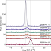 |
Fig. A.2 22 GHz H2O maser spectra obtained toward Gy 3–7 with the 32-m radio telescope in Torun from December 2019 to May 2020. The date of observations is indicated above each spectrum. Except for the spectrum corresponding to the observation on May 15, 2020, spectra are shifted vertically by 30 Jy (for the observation on March 21, 2020) and 15 Jy (for the remaining observations) to improve the clarity of the figure. Dashed vertical lines show central velocities of the lines detected in the latest (May 15, 2020) and earliest (December 11, 2019) of the six epochs of observations (see also Table A.1). |
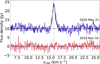 |
Fig. A.3 22 GHz H2O maser emission detected toward IRAS 07069–1026 (see also Table A.1). The H2O maser was detected only in one of the two observing epochs. The spectrum observed on May 21, 2020 is shifted vertically by 10 Jy to improve the clarity of the figure. |
The Gauss functions were fitted to the 22 GHz water maser lines observed towards Gy 3–7 and IRAS 07069–1026. The Gauss fitting results are shown Table A.1: the central velocities (Vp) of the water maser lines, their peak flux densities (Sp), full-widths at half maximum (FWHM), and the integrated flux densities (∫ SdV). The measured flux densities are likely underestimated by 10–20% due to the atmospheric conditions at the observatory site; no correction for atmospheric attenuation was applied.
Parameters of the 22 GHz H2O maser lines detected toward CMa–l224 with RT4
Appendix A.2: Water maser emission in Gy 3–7
Urquhart et al. (2011) report the detection of a single water maser spot toward Gy 3–7 (G224.6075–01.0063) with the peak flux density of 2.57 Jy and velocity of 28.7 km s−1 (~25 km s−1 higher than the emission detected with RT4). However, the inspection of the spectrum provided by Urquhart et al. (2011) reveals a second, much fainter and broader water maser line centered at the velocity of ~0 km s−1, only ~2–4 km s−1 lower than the peak velocities of the lines detected in our observations. No water maser emission at higher velocities was detected in any of the six RT4 epochs.
The systemic velocity of Gy 3–7 is 16.7 km s−1 based on the NH3 observations of Urquhart et al. (2011), in a very good agreement with the CO 1–0 velocity of ~16 km s−1 (Benedettini et al. 2020), indicating that NH3 and CO trace the same molecular gas. The water maser emission toward Gy 3–7 is blueshifted (this study) and redshifted (Urquhart et al. 2011) with respect to the systemic velocity. The blueshifted emission has the similar velocity offset (~13–16 km s−1) from the systemic velocity as the redshifted emission (12 km s−1), extending the velocity range over which the maser spots are found toward Gy 3–7 from ~2 km s−1 reported in Urquhart et al. (2011) to ~30 km s−1.
About 60% of the sources from the Urquhart et al. (2011) sample have total velocity ranges of the water maser emission of ≲20 km s−1. The mean/median velocity range of the entire sample is 24.7/15.2 km s−1. Six sources have velocity ranges of >100 km s−1. The Gy 3–7’s water maser velocity range of ~30 km s−1 is larger than the velocity ranges of the majority of the sources from the Urquhart et al. (2011) sample, but it is well within the observed values.
The water maser data currently available for Gy 3–7 show that the blueshifted water maser spots are brighter than the red-shitfed ones (and thus detected more often), in agreement with the results obtained by Urquhart et al. (2011) for a large sample of ~300 YSOs and H II regions. The higher relative velocities of blueshifted masers also agree with the Urquhart et al. (2011)’ results.
The difference of ~12–16 km s−1 between the systemic velocity of Gy 3–7 and the velocities of maser spots is small enough to assume that there is the physical association between the molecular gas traced by NH3 and CO and the maser emission (possibly originating in outflow shocks); it is less likely that the maser emission is arising from a different region located along the same line of sight. The mean difference between the maser and systemic velocities for the Urquhart et al. (2011) sample of YSOs and HII regions is −3.8 km s−1, but with the large standard deviation (~20 km s−1). It is possible that the water maser emission with smaller offsets from the systemic velocity of Gy 3–7 exists, but remained undetected due to the maser variability and/or limited sensitivity of the observations.
The spatial resolution of the existing water maser observations of Gy 3–7 is too low to accurately pinpoint the location of the maser spots in the region. Higher resolution observations are needed to investigate the distribution of the maser spots toward Gy 3–7 and the origin of the maser emission. Systematic monitoring of the water maser activity at high angular resolution would be necessary to constrain any periodicity in the maser line intensity in one or more velocity components (Szymczak et al. 2016).
Appendix B Spatial extent of FIR line emission
Figures B.1 and B.2 show the spatial extent of the [O I] lines at 63 and 145 μm, the [C II] line at 157 μm, the CO lines with Jup = 14 – 31, and the OH line at 79.2 μm. We calculated the flux of these emission line toward the two dense cores A and B, within a beam size of 20″ (Table B.1). Since all lines are spectrally-unresolved, the line fluxes are obtained using Gaussian fits and their uncertainties are estimated as 1σ of the distribution of 10 000 Gaussian profiles generated based on the parameters of the Gaussian fit and their uncertainty.
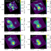 |
Fig. B.1 FIFI-LS integrated intensity maps of the [O I] lines at 63.2 and 145.5 μm, the [C II] line at 157.7 μm, the CO lines J = 14 – 13, 16 – 15, 17 – 16 at 186, 162.8, 153.3 μm, respectively. The white contours show line emission at 25%, 50%, 75%, and 95% of the corresponding line emission peak. The “+” and “x” signs show the positions of the dense cores A and B, respectively. |
Flux SOFIA FIFI-LS toward the two dense cores within a beam size of 20”.
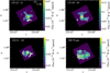 |
Fig. B.2 FIFI-LS integrated intensity maps of the CO 22 – 21, CO 30 – 29, and CO 31 – 30 transitions at 118, 84, and 87 μm, respectively, and the OH line at 79.2 μm. The white contours show line emission at 25%, 50%, 75%, and 95% of the corresponding line emission peak, see also Figure B.1. |
Appendix C Multi-wavelength photometry and SED fitting results
Table C.1 shows the multi-wavelength photometry for 15 YSO candidates in Gy 3–7. Figure C.1 shows the SEDs of YSO candidates in Gy 3–7 with the best-fit Robitaille (2017) models. Figure C.2 shows the Hertzsprung-Russell diagram with the positions of the YSOs obtained from the SED modeling in line with the PMS tracks.
We note that sources numbered 3 – 8 and source 11 lack continuum measurements at > 4.5 μm, which limits the SED modeling. The best-fit models for sources No. 4–6 and 11 are stars (Table 4), since the envelope emission could not be traced. Near-IR observations show some IR excess toward source No. 6 (Tapia et al. 1997), but the confirmation of its YSO status would require additional observations, which are outside of the scope of this paper.
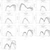 |
Fig. C.1 SEDs of YSO candidates with well-fitted Robitaille (2017) YSO models. The best-fit model is indicated with the black solid line. Gray lines show the YSO models with χ2 between |


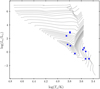 |
Fig. C.2 HR diagram with YSOs in Gy 3–7 (blue ‘×’ symbols) and the PARSEC evolutionary tracks (Bressan et al. 2012; Chen et al. 2014, 2015; Tang et al. 2014). |
Multi-wavelength photometry of YSO candidates in the IRAS field. The columns represent the 2MASS JHKs, Spitzer IRAC 3.6 and 4.5 μm, AllWISE, Herschel PACS, and SPIRE
Appendix D CO rotational temperature of the intermediate-to high-mass YSOs in the Milky Way
We compare the rotational temperatures towards the two dense cores to the results found in the samples of the IM and HM YSOs in the Milky Way. There are six IM and ten HM YSOs presented in Karska et al. (2014a) and Matuszak et al. (2015), respectively using the data from Herschel/PACS. To be consistent with our SOFIA/FIFI-LS data, we recalculated the rotational temperatures derived by fitting the rotational diagram using 4 CO transitions with Jup = (14, 16, 18, 22) and (14, 16, 17, 22) for the IM and HM YSOs, respectively.
We checked the new results with the ones presented in the aforementioned studies and find that using only four CO transitions returns a lower Trot than the case of using all the observable CO transitions. The relative difference is in between 4-27% with a median of 5% for the HM YSOs. The comparison of these differences is shown in Table D.1.
Table D.2 shows heliocentric distances, Galactocentric radii, metallicities, and luminosities of the sources in the Milky Way and Magellanic Clouds. We used heliocentric distances together with source coordinates to calculate Galactocentric radii, assuming a distance from the Sun to the Galactic center of 8.34 kpc. We estimated the metallicity toward the Milky Way sources using the O/H galactocentric radial gradient based on H II regions in the Galactic disk (Balser et al. 2011).
CO rotational temperature and number of emitting molecules for HM YSOs, derived by fitting the rotational diagram of CO using all and only four available CO transitions.
FIR line cooling luminosity of the sample in the Milky Way (MW), LMC, and SMC used to compare with results of this study
References
- Arce, H. G., Shepherd, D., Gueth, F., et al. 2007, in Protostars and Planets V, eds. B. Reipurth, D. Jewitt, & K. Keil (Tucson: University of Arizona Press), 245 [Google Scholar]
- Balser, D. S., Rood, R. T., Bania, T. M., & Anderson, L. D. 2011, ApJ, 738, 27 [NASA ADS] [CrossRef] [Google Scholar]
- Benedettini, M., Molinari, S., Baldeschi, A., et al. 2020, A&A, 633, A147 [NASA ADS] [CrossRef] [EDP Sciences] [Google Scholar]
- Benz, A. O., Bruderer, S., van Dishoeck, E. F., et al. 2016, A&A, 590, A105 [NASA ADS] [CrossRef] [EDP Sciences] [Google Scholar]
- Bica, E., Dutra, C. M., & Barbuy, B. 2003, A&A, 397, 177 [NASA ADS] [CrossRef] [EDP Sciences] [Google Scholar]
- Bressan, A., Marigo, P., Girardi, L., et al. 2012, MNRAS, 427, 127 [NASA ADS] [CrossRef] [Google Scholar]
- Bronfman, L., Nyman, L. A., & May, J. 1996, A&AS, 115, 81 [Google Scholar]
- Bruderer, S., Benz, A. O., Doty, S. D., van Dishoeck, E. F., & Bourke, T. L. 2009, ApJ, 700, 872 [NASA ADS] [CrossRef] [Google Scholar]
- Butner, H. M., Evans J., Neal, I., Harvey, P.M., et al. 1990, ApJ, 364, 164 [NASA ADS] [CrossRef] [Google Scholar]
- Chen, Y., Girardi, L., Bressan, A., et al. 2014, MNRAS, 444, 2525 [Google Scholar]
- Chen, Y., Bressan, A., Girardi, L., et al. 2015, MNRAS, 452, 1068 [Google Scholar]
- Cyganowski, C. J., Whitney, B. A., Holden, E., et al. 2008, AJ, 136, 2391 [Google Scholar]
- Cyganowski, C. J., Brogan, C. L., Hunter, T. R., Churchwell, E., & Zhang, Q. 2011, ApJ, 729, 124 [NASA ADS] [CrossRef] [Google Scholar]
- Dunham, M. M., Allen, L. E., Evans J., Neal I., et al. 2015, ApJS, 220, 11 [NASA ADS] [CrossRef] [Google Scholar]
- Elia, D., Molinari, S., Fukui, Y., et al. 2013, ApJ, 772, 45 [NASA ADS] [CrossRef] [Google Scholar]
- Elia, D., Merello, M., Molinari, S., et al. 2021, MNRAS, 504, 2742 [NASA ADS] [CrossRef] [Google Scholar]
- Elitzur, M., Hollenbach, D. J., & McKee, C. F. 1989, ApJ, 346, 983 [NASA ADS] [CrossRef] [Google Scholar]
- Esteban, C., & García-Rojas, J. 2018, MNRAS, 478, 2315 [NASA ADS] [CrossRef] [Google Scholar]
- Faúndez, S., Bronfman, L., Garay, G., et al. 2004, A&A, 426, 97 [Google Scholar]
- Fernández-Martín, A., Pérez-Montero, E., Vílchez, J. M., & Mampaso, A. 2017, A&A, 597, A84 [NASA ADS] [CrossRef] [EDP Sciences] [Google Scholar]
- Fischer, C., Beckmann, S., Bryant, A., et al. 2018, J. Astron. Instrum., 7, 1840003 [Google Scholar]
- Fischer, C., Iserlohe, C., Vacca, W., et al. 2021, PASP, 133, 055001 [NASA ADS] [CrossRef] [Google Scholar]
- Flower, D. R., & Pineau des Forêts, G. 2012, MNRAS, 421, 2786 [NASA ADS] [CrossRef] [Google Scholar]
- Frank, A., Ray, T. P., Cabrit, S., et al. 2014, in Protostars and Planets VI, eds. H. Beuther, R.S. Klessen, C. P. Dullemond, & T. Henning (Tucson: University of Arizona Press), 451 [Google Scholar]
- Furuya, R. S., Kitamura, Y., Wootten, A., Claussen, M. J., & Kawabe, R. 2003, ApJS, 144, 71 [NASA ADS] [CrossRef] [Google Scholar]
- Giannini, T., Massi, F., Podio, L., et al. 2005, A&A, 433, 941 [NASA ADS] [CrossRef] [EDP Sciences] [Google Scholar]
- Goicoechea, J. R., Cernicharo, J., Karska, A., et al. 2012, A&A, 548, A77 [NASA ADS] [CrossRef] [EDP Sciences] [Google Scholar]
- Goldsmith, P. F., & Langer, W. D. 1978, ApJ, 222, 881 [Google Scholar]
- Goldsmith, P. F., & Langer, W. D. 1999, ApJ, 517, 209 [Google Scholar]
- Graczyk, D., Pietrzyński, G., Thompson, I. B., et al. 2014, ApJ, 780, 59 [Google Scholar]
- Green, J. D., Evans I., Neal J., Jørgensen, J. K., et al. 2013, ApJ, 770, 123 [NASA ADS] [CrossRef] [Google Scholar]
- Green, J. D., Yang, Y.-L., Evans I., Neal J., et al. 2016, AJ, 151, 75 [NASA ADS] [CrossRef] [Google Scholar]
- Griffin, M. J., Abergel, A., Abreu, A., et al. 2010, A&A, 518, A3 [Google Scholar]
- Guevara, C., Stutzki, J., Ossenkopf-Okada, V., et al. 2020, A&A, 636, A16 [CrossRef] [EDP Sciences] [Google Scholar]
- Gyulbudaghian, A. L. 2012, Astrophysics, 55, 92 [Google Scholar]
- Habing, H. J. 1968, Bull. Astron. Inst. Netherlands, 19, 421 [Google Scholar]
- Hachisuka, K., Brunthaler, A., Menten, K. M., et al. 2006, ApJ, 645, 337 [NASA ADS] [CrossRef] [Google Scholar]
- Hatchell, J., & van der Tak, F. F. S. 2003, A&A, 409, 589 [NASA ADS] [CrossRef] [EDP Sciences] [Google Scholar]
- He, J. H., Takahashi, S., & Chen, X. 2012, ApJS, 202, 1 [NASA ADS] [CrossRef] [Google Scholar]
- Herczeg, G. J., Karska, A., Bruderer, S., et al. 2012, A&A, 540, A84 [NASA ADS] [CrossRef] [EDP Sciences] [Google Scholar]
- Heyer, M., & Dame, T. M. 2015, ARA&A, 53, 583 [Google Scholar]
- Hollenbach, D., & McKee, C. F. 1989, ApJ, 342, 306 [Google Scholar]
- Hollenbach, D. J., & Tielens, A. G. G. M. 1997, ARA&A, 35, 179 [NASA ADS] [CrossRef] [Google Scholar]
- Immer, K., Reid, M. J., Menten, K. M., Brunthaler, A., & Dame, T. M. 2013, A&A, 553, A117 [NASA ADS] [CrossRef] [EDP Sciences] [Google Scholar]
- Iserlohe, C., Fischer, C., Vacca, W. D., et al. 2021, PASP, 133, 055002 [NASA ADS] [CrossRef] [Google Scholar]
- Jakob, H., Kramer, C., Simon, R., et al. 2007, A&A, 461, 999 [NASA ADS] [CrossRef] [EDP Sciences] [Google Scholar]
- Jiménez-Donaire, M. J., Meeus, G., Karska, A., et al. 2017, A&A, 605, A62 [NASA ADS] [CrossRef] [EDP Sciences] [Google Scholar]
- Johnstone, D., Fich, M., McCoey, C., et al. 2010, A&A, 521, A41 [Google Scholar]
- Karska, A., Herczeg, G. J., van Dishoeck, E. F., et al. 2013, A&A, 552, A141 [NASA ADS] [CrossRef] [EDP Sciences] [Google Scholar]
- Karska, A., Herpin, F., Bruderer, S., et al. 2014a, A&A, 562, A45 [NASA ADS] [CrossRef] [EDP Sciences] [Google Scholar]
- Karska, A., Kristensen, L. E., van Dishoeck, E. F., et al. 2014b, A&A, 572, A9 [NASA ADS] [CrossRef] [EDP Sciences] [Google Scholar]
- Karska, A., Kaufman, M. J., Kristensen, L. E., et al. 2018, ApJS, 235, 30 [NASA ADS] [CrossRef] [Google Scholar]
- Karska, A., Koprowski, M., Solarz, A., et al. 2022, A&A, 663, A133 [NASA ADS] [CrossRef] [EDP Sciences] [Google Scholar]
- Kaufman, M. J., & Neufeld, D. A. 1996, ApJ, 456, 611 [NASA ADS] [CrossRef] [Google Scholar]
- Kaufman, M. J., Wolfire, M. G., & Hollenbach, D. J. 2006, ApJ, 644, 283 [Google Scholar]
- Klein, R., Beckmann, S., Bryant, A., et al. 2014, SPIE Conf. Ser., 9147, 91472X [NASA ADS] [Google Scholar]
- Kristensen, L. E., van Dishoeck, E. F., Bergin, E. A., et al. 2012, A&A, 542, A8 [NASA ADS] [CrossRef] [EDP Sciences] [Google Scholar]
- Kristensen, L. E., Gusdorf, A., Mottram, J. C., et al. 2017a, A&A, 601, A4 [Google Scholar]
- Kristensen, L. E., van Dishoeck, E. F., Mottram, J. C., et al. 2017b, A&A, 605, A93 [NASA ADS] [CrossRef] [EDP Sciences] [Google Scholar]
- Kuchar, T. A., & Bania, T. M. 1994, ApJ, 436, 117 [NASA ADS] [CrossRef] [Google Scholar]
- Ladd, E. F., Deane, J. R., Sanders, D. B., & Wynn-Williams, C. G. 1993, ApJ, 419, 186 [NASA ADS] [CrossRef] [Google Scholar]
- Ladeyschikov, D. A., Gong, Y., Sobolev, A. M., et al. 2022, ApJS, 261, 14 [NASA ADS] [CrossRef] [Google Scholar]
- Leurini, S., Wyrowski, F., Wiesemeyer, H., et al. 2015, A&A, 584, A70 [NASA ADS] [CrossRef] [EDP Sciences] [Google Scholar]
- Lew, B. 2018, Exp. Astron., 45, 81 [NASA ADS] [CrossRef] [Google Scholar]
- Liseau, R., Lorenzetti, D., Nisini, B., Spinoglio, L., & Moneti, A. 1992, A&A, 265, 577 [NASA ADS] [Google Scholar]
- Litvak, M. M. 1969, Science, 165, 855 [NASA ADS] [CrossRef] [Google Scholar]
- Lombardi, M., Alves, J., & Lada, C. J. 2011, A&A, 535, A16 [NASA ADS] [CrossRef] [EDP Sciences] [Google Scholar]
- Manoj, P., Watson, D. M., Neufeld, D. A., et al. 2013, ApJ, 763, 83 [NASA ADS] [CrossRef] [Google Scholar]
- Marsh, K. A., Whitworth, A. P., Lomax, O., et al. 2017, MNRAS, 471, 2730 [Google Scholar]
- Matuszak, M., Karska, A., Kristensen, L. E., et al. 2015, A&A., 578, A20 [NASA ADS] [CrossRef] [EDP Sciences] [Google Scholar]
- Melnick, G. J., & Kaufman, M. J. 2015, ApJ, 806, 227 [NASA ADS] [CrossRef] [Google Scholar]
- Menten, K. M., Reid, M. J., Pratap, P., Moran, J. M., & Wilson, T. L. 1992, ApJ, 401, L39 [NASA ADS] [CrossRef] [Google Scholar]
- Minier, V., André, P., Bergman, P., et al. 2009, A&A, 501, L1 [NASA ADS] [CrossRef] [EDP Sciences] [Google Scholar]
- Mirocha, A., Karska, A., Gronowski, M., et al. 2021, A&A, 656, A146 [NASA ADS] [CrossRef] [EDP Sciences] [Google Scholar]
- Molinari, S., Swinyard, B., Bally, J., et al. 2010, A&A, 518, A100 [Google Scholar]
- Mookerjea, B., Sandell, G., Veena, V. S., et al. 2021, A&A, 648, A40 [NASA ADS] [CrossRef] [EDP Sciences] [Google Scholar]
- Moscadelli, L., Reid, M. J., Menten, K. M., et al. 2009, ApJ, 693, 406 [NASA ADS] [CrossRef] [Google Scholar]
- Motogi, K., Sorai, K., Habe, A., et al. 2011, PASJ, 63, 31 [NASA ADS] [Google Scholar]
- Mottram, J. C., van Dishoeck, E. F., Kristensen, L. E., et al. 2017, A&A, 600, A99 [NASA ADS] [CrossRef] [EDP Sciences] [Google Scholar]
- Navarete, F., Damineli, A., Barbosa, C. L., & Blum, R. D. 2015, MNRAS, 450, 4364 [NASA ADS] [CrossRef] [Google Scholar]
- Neckel, T. 1978, A&A, 69, 51 [NASA ADS] [Google Scholar]
- Nisini, B., Santangelo, G., Giannini, T., et al. 2015, ApJ, 801, 121 [NASA ADS] [CrossRef] [Google Scholar]
- Oliveira, J. M., van Loon, J. T., Sewiło, M., et al. 2019, MNRAS, 490, 3909 [NASA ADS] [CrossRef] [Google Scholar]
- Ossenkopf, V., Röllig, M., Simon, R., et al. 2010, A&A, 518, A79 [Google Scholar]
- Pickett, H. M., Poynter, R. L., Cohen, E. A., et al. 1998, J. Quant. Spec. Radiat. Transf., 60, 883 [Google Scholar]
- Pietrzyński, G., Graczyk, D., Gieren, W., et al. 2013, Nature, 495, 76 [Google Scholar]
- Pilbratt, G. L., Riedinger, J. R., Passvogel, T., et al. 2010, A&A, 518, A1 [NASA ADS] [CrossRef] [EDP Sciences] [Google Scholar]
- Poglitsch, A., Waelkens, C., Geis, N., et al. 2010, A&A, 518, A2 [Google Scholar]
- Pound, M. W., & Wolfire, M. G. 2011, ASP Conf. Ser., 394, 654 [Google Scholar]
- Purser, S. J. D., Lumsden, S. L., Hoare, M. G., & Kurtz, S. 2021, MNRAS, 504, 338 [NASA ADS] [CrossRef] [Google Scholar]
- Risacher, C., Güsten, R., Stutzki, J., et al. 2018, J. Astron. Instrum., 7, 1840014 [NASA ADS] [CrossRef] [Google Scholar]
- Robitaille, T. P. 2017, A&A, 600, A11 [NASA ADS] [CrossRef] [EDP Sciences] [Google Scholar]
- Robitaille, T. P., Whitney, B. A., Indebetouw, R., & Wood, K. 2007, ApJS, 169, 328 [Google Scholar]
- Roman-Duval, J., Jackson, J. M., Heyer, M., Rathborne, J., & Simon, R. 2010, ApJ, 723, 492 [NASA ADS] [CrossRef] [Google Scholar]
- Russell, S. C., & Dopita, M. A. 1992, ApJ, 384, 508 [NASA ADS] [CrossRef] [Google Scholar]
- Rygl, K. L. J., Brunthaler, A., Sanna, A., et al. 2012, A&A, 539, A79 [NASA ADS] [CrossRef] [EDP Sciences] [Google Scholar]
- Sandell, G. 2000, A&A, 358, 242 [NASA ADS] [Google Scholar]
- Sandell, G., & Sievers, A. 2004, ApJ, 600, 269 [NASA ADS] [CrossRef] [Google Scholar]
- Schöier, F. L., van der Tak, F. F. S., van Dishoeck, E. F., & Black, J. H. 2005, A&A, 432, 369 [Google Scholar]
- Sewiło, M., Whitney, B. A., Yung, B. H. K., et al. 2019, ApJS, 240, 26 [CrossRef] [Google Scholar]
- Shevchenko, V. S., & Yakubov, S. D. 1989, Soviet Ast., 33, 370 [NASA ADS] [Google Scholar]
- Soares, J. B., & Bica, E. 2002, A&A, 388, 172 [NASA ADS] [CrossRef] [EDP Sciences] [Google Scholar]
- Soares, J. B., & Bica, E. 2003, A&A, 404, 217 [NASA ADS] [CrossRef] [EDP Sciences] [Google Scholar]
- Sodroski, T. J., Odegard, N., Arendt, R. G., et al. 1997, ApJ, 480, 173 [NASA ADS] [CrossRef] [Google Scholar]
- Stanke, T., McCaughrean, M. J., & Zinnecker, H. 2000, A&A, 355, 639 [NASA ADS] [Google Scholar]
- Szymczak, M., Hrynek, G., & Kus, A. J. 2000, A&AS 143, 269 [NASA ADS] [CrossRef] [EDP Sciences] [Google Scholar]
- Szymczak, M., Olech, M., Wolak, P., Bartkiewicz, A., & Gawroński, M. 2016, MNRAS, 459, L56 [NASA ADS] [CrossRef] [Google Scholar]
- Tang, J., Bressan, A., Rosenfield, P., et al. 2014, MNRAS, 445, 4287 [NASA ADS] [CrossRef] [Google Scholar]
- Tapia, M., Persi, P., Bohigas, J., & Ferrari-Toniolo, M. 1997, AJ, 113, 1769 [Google Scholar]
- Tobin, J. J., Stutz, A. M., Manoj, P., et al. 2016, ApJ, 831, 36 [NASA ADS] [CrossRef] [Google Scholar]
- Urquhart, J. S., Morgan, L. K., Figura, C. C., et al. 2011, MNRAS, 418, 1689 [NASA ADS] [CrossRef] [Google Scholar]
- Urquhart, J. S., Hoare, M. G., Lumsden, S. L., et al. 2012, MNRAS, 420, 1656 [NASA ADS] [CrossRef] [Google Scholar]
- Vacca, W., Clarke, M., Perera, D., Fadda, D., & Holt, J. 2020, ASP Conf. Ser., 527, 547 [NASA ADS] [Google Scholar]
- Valdettaro, R., Palla, F., Brand, J., et al. 2001, A&A, 368, 845 [CrossRef] [EDP Sciences] [Google Scholar]
- van der Tak, F. F. S. 2012, Philos. Trans. Roy. Soc. Lond. A., 370, 5186 [NASA ADS] [Google Scholar]
- van der Tak, F. F. S., van Dishoeck, E. F., Evans, N. J. II, Bakker, E. J., & Blake, G. A. 1999, ApJ, 522, 991 [NASA ADS] [CrossRef] [Google Scholar]
- van Dishoeck, E. F., Kristensen, L. E., Benz, A. O., et al. 2011, PASP, 123, 138 [NASA ADS] [CrossRef] [Google Scholar]
- van Dishoeck, E. F., Kristensen, L. E., Mottram, J. C., et al. 2021, A&A, 648, A24 [NASA ADS] [CrossRef] [EDP Sciences] [Google Scholar]
- Visser, R., Kristensen, L. E., Bruderer, S., et al. 2012, A&A, 537, A55 [NASA ADS] [CrossRef] [EDP Sciences] [Google Scholar]
- White, G. J., Abergel, A., Spencer, L., et al. 2010, A&A, 518, A114 [Google Scholar]
- Wiesenfeld, L., & Goldsmith, P. F. 2014, ApJ, 780, 183 [Google Scholar]
- Wilson, B. A., Dame, T. M., Masheder, M. R. W., & Thaddeus, P. 2005, A&A, 430, 523 [NASA ADS] [CrossRef] [EDP Sciences] [Google Scholar]
- Wood, D. O. S., & Churchwell, E. 1989, ApJ, 340, 265 [NASA ADS] [CrossRef] [Google Scholar]
- Wouterloot, J. G. A., & Brand, J. 1989, A&AS, 80, 149 [NASA ADS] [Google Scholar]
- Xu, Y., Reid, M. J., Menten, K. M., et al. 2009, ApJ, 693, 413 [CrossRef] [Google Scholar]
- Yang, Y.-L., Green, J. D., Evans I., Neal J., et al. 2018, ApJ, 860, 174 [NASA ADS] [CrossRef] [Google Scholar]
- Yang, Y.-L., Evans, N. J., Karska, A., et al. 2022a, ApJ, 925, 93 [NASA ADS] [CrossRef] [Google Scholar]
- Yang, Y.-L., Green, J. D., Pontoppidan, K. M., et al. 2022b, ApJ, 941, L13 [NASA ADS] [CrossRef] [Google Scholar]
All Tables
CO rotational temperature, the number of emitting molecules, and total line luminosities of CO and [O I] lines toward dense cores in Gy 3–7 and IM YSOs from Matuszak et al. (2015).
Physical parameters for a subset of YSO candidates with at least five photometric data points.
Multi-wavelength photometry of YSO candidates in the IRAS field. The columns represent the 2MASS JHKs, Spitzer IRAC 3.6 and 4.5 μm, AllWISE, Herschel PACS, and SPIRE
CO rotational temperature and number of emitting molecules for HM YSOs, derived by fitting the rotational diagram of CO using all and only four available CO transitions.
FIR line cooling luminosity of the sample in the Milky Way (MW), LMC, and SMC used to compare with results of this study
All Figures
|
Fig. 1 Digital Sky Survey (DSS) R (top left), 2MASS composite image using the J, H, and Ks filters (top right), Spfeer/GLIMPSE360 4.5 μm (Sewiło et al. 2019; bottom left), and Herschel/Hi-GAL composite image at 70, 160, and 250 μm (Elia et al. 2013; bottom right) of the Gy 3–7 cluster. Circles in the top panels show the positions of YSO candidates from Tapia et al. (1997). Yellow diamond and red cross in the bottom-left panel show the position of the H2O maser (Urquhart et al. 2011) and the IRAS source at the south-west side (IRAS 07069–1045), respectively. The blue “×” symbols in the bottom right panel show the positions of dense cores as traced by the H2 column density (Elia et al. 2013). Dense core in the west corresponds to IRAS 07069-1045. |
| In the text | |
|
Fig. 2 Distribution of dust continuum emission toward Gy 3–7. Left: continuum map of Gy 3–7 at 70 μm observed with Herschel/PACS. Red “+” and blue “×” symbols refer to the 70 μm continuum peaks, adopted as the positions for the dense cores A and B in the subsequent analysis. Circles show the positions of HIGALBM224.6079–1.0065 and HIGALBM224.6128–1.0013 cores from the Herschel/Hi-GAL catalog (Elia et al. 2021). Right: map of the H2 column density (NH2). Black circles with the beam size of 20″ indicate the extract regions of the SOFIA FIFI-LS spectra toward the two dense cores A and B (see more in Sect. 3.1). White contours in each map show the continuum at 70 μm, with contour levels at 5, 10, 40, 80, 400, and 800 mJy arcsec−2. |
| In the text | |
|
Fig. 3 SOFIA FIFI-LS continuum-subtracted spectra toward the two dense cores in Gy 3–7: HIGALBM224.6079–1.0065 (source “A”) and HIGALBM224.6128–1.0013 (source “B”). The emission is extracted within a beam size of 20″ indicated by black circles in the right panel of Fig. 2. Vertical lines show the laboratory wavelengths of the detected lines. Spectra of the [OI] line at 63 μm are multiplied by a factor of 0.2 and those of the CO 14–13 line by a factor of 0.6 to better illustrate the line detections. |
| In the text | |
|
Fig. 4 FIFI-LS contour maps of the [O I] lines at 63.2 and 145.5 μm, the [CII] line at 157.7 μm, the CO lines with Jup = 14, 16, 17 at 186, 163, and 153 μm respectively (white contours) on top of the continuum emission at 160 μm (at 70 μm for the [OI] line at 63.2 μm) from Herschel/PACS. The white contours show line emission at 25%, 50%, 75%, and 95% of the corresponding line emission peak. The “+” and “×” signs show the positions of the dense cores A and B. |
| In the text | |
|
Fig. 5 FIFI-LS contour maps of the [O I] lines at 63.2 and 145.5 μm, the [CII] line at 157.7 μm, and the CO 14-13 line at 186 μm (white contours) on top of the continuum emission at 4.5 μm from Spitzer/IRAC. The contours show line emission at 25%, 50%, 75%, and 95% of the corresponding line emission peak. The “+” and “×” signs show the positions of the dense cores A and B, respectively. The orange squares show the positions of two YSO candidates with envelopes, and the yellow circles show the positions of the remaining YSOs (Sect. 4.5). |
| In the text | |
|
Fig. 6 Integrated intensity maps of selected pairs of FIR lines from FIFI-LS with the top line shown in colors, and the bottom line in white contours. The contour levels are 25%, 50%, 75%, and 95% of the corresponding line emission peak. The “+” and “×” signs show the positions of the dense cores A and B, respectively. The spaxel size in the emission map of the [O I] line at 63 μm is 6″ × 6″ (blue channel) and in the map of other lines (CO 14-13, [OI] at 145 μm, and [CII] at 157.7 μm) is 12″ × 12″ (red channel). Gray circles show the beam size for each color map. |
| In the text | |
|
Fig. 7 CO rotational diagrams toward core A (left, in blue) and B (right, in orange). Circles refer to values based on line detections and the triangle shows the measurement using the upper limit of the CO 31-30 line, which is blended with OH. Solid lines show fits using transitions belonging to the “warm” gas component; the CO 30–29 line at 87.19 μm is therefore not included. The CO rotational temperature Trot derived from the rotational diagram is labeled in each panel and the value in parenthesis indicates its uncertainty. |
| In the text | |
|
Fig. 8 Gas and dust temperatures toward Gy 3–7. Left: CO rotational temperature map obtained using Boltzmann diagrams. White contour map shows the CO 17–16 emission at 25%, 50%, 75%, and 95% of the emission peak. Right: H2 column density contour map overlaid on the dust temperature map derived from the ppmap tool with the Herschel/Hi-GAL survey (Marsh et al. 2017). Contour levels of the N(H2) are at (5, 10, 30, 50, 55) × 1021 cm−2. |
| In the text | |
|
Fig. 9 Spatial extent of FIR line luminosities of CO (left) and [O I] (right) toward Gy 3–7. The calculation procedure is described in Sect. 4.2. |
| In the text | |
|
Fig. 10 Correlations between luminosities of FIR CO and [O I] lines. Top: correlation between the luminosities of the 63 and 145 μm [O I] lines at from LM to HM YSOs. Cores A and B in Gy 3–7 are marked as grey diamonds, Class 0 and Class I YSOs as orange "×" signs and red circles (Karska et al. 2018), respectively, IM YSOs as blue circles (Matuszak et al. 2015), and HM YSOs as green squares, respectively (Karska et al. 2014a). Black solid line is the linear fit to all sources except for the HM YSOs, showing a strong correlation between the two [O I] line luminosities. Bottom: correlation between luminosities of the CO lines and the [O I] line at 145 μm. Black solid line shows the linear fit to all sources, including the HM YSOs. |
| In the text | |
|
Fig. 11 Ratio of the CO and [O I] luminosities as a function of preshock density for UV irradiated C–shock models and observations of Gy 3-7 cores and IM YSOs from Matuszak et al. (2015; light blue box). All models correspond to UV fields parameterized by G0 of 10 (in blue) and 0.1 (in orange). Solid lines connect models with shock velocities vs of 20 km s−1, and dashed lines – the models with vs of 10 km s−1. |
| In the text | |
|
Fig. 12 SEDs of YSOs in Gy 3-7 well-fitted with Robitaille (2017) models with envelopes. The best fit model is indicated with the black solid line and gray lines show the YSO models with χ2 between |
| In the text | |
|
Fig. 13 CO rotational temperatures for dense cores in Gy 3–7 and intermediate- and high-mass YSOs from the literature (Karska et al. 2014a; Matuszak et al. 2015). Top: straightforward comparison with the literature values. Bottom: Comparison accounting for the number of observed CO lines considered in the rotational diagrams. |
| In the text | |
|
Fig. 14 Correlations between the ratio of CO and [O I] line luminosities and bolometric luminosity of YSOs in the two cores in Gy 3–7 (gray diamonds), Class 0 and Class I YSOs (orange ‘×’ signs and red circles, respectively; Karska et al. 2018), IM YSOs (blue circles; Matuszak et al. 2015), and HM YSOs (green squares; Karska et al. 2014a). The bolometric luminosities for Gy 3–7 cores are adopted from Elia et al. (2021). The top panel shows a power-law fit to all individual data points, and the bottom panel shows the fit to the data bins (both shown as black dashed line). |
| In the text | |
|
Fig. 15 Ratio of molecular to atomic line luminosities as a function of the Galactocentric radius. The light coral box indicates the range of the line luminosity ratio and the Galactocentric radius for LM YSOs in the nearby clouds, which are excluded from the power-law fit to the remaining YSOs (dashed black line). Gray dotted horizontal line indicates where the molecular luminosity is equal to the atomic luminosity. |
| In the text | |
|
Fig. 16 Ratio of molecular to atomic line luminosities as a function of metallicity, Z. HM YSOs in the SMC and LMC are shown with cross and “×” symbols in orange and purple colors, respectively. The light coral box indicates the range of the line luminosity ratio and the metallicity for LM YSOs in the nearby clouds, which are excluded from the power-law fit to the remaining YSOs (dashed black line). The gray dotted horizontal line indicates where the molecular luminosity is equal to the atomic luminosity. |
| In the text | |
|
Fig. A.1 CO 1 – 0 integrated intensity map of CMa-l224. Yellow circles show all RT4 pointings, while white circles indicate those with the 22 GHz water maser detections: toward Gy 3–7 and source IRAS 07069–1026 in the main filament. Blue and red circles indicate the positions of water masers detected toward CMa–l224 with the GBT (Urquhart et al. 2011) and the Medicina telescope (Valdettaro et al. 2001), respectively (see text for details). |
| In the text | |
|
Fig. A.2 22 GHz H2O maser spectra obtained toward Gy 3–7 with the 32-m radio telescope in Torun from December 2019 to May 2020. The date of observations is indicated above each spectrum. Except for the spectrum corresponding to the observation on May 15, 2020, spectra are shifted vertically by 30 Jy (for the observation on March 21, 2020) and 15 Jy (for the remaining observations) to improve the clarity of the figure. Dashed vertical lines show central velocities of the lines detected in the latest (May 15, 2020) and earliest (December 11, 2019) of the six epochs of observations (see also Table A.1). |
| In the text | |
|
Fig. A.3 22 GHz H2O maser emission detected toward IRAS 07069–1026 (see also Table A.1). The H2O maser was detected only in one of the two observing epochs. The spectrum observed on May 21, 2020 is shifted vertically by 10 Jy to improve the clarity of the figure. |
| In the text | |
|
Fig. B.1 FIFI-LS integrated intensity maps of the [O I] lines at 63.2 and 145.5 μm, the [C II] line at 157.7 μm, the CO lines J = 14 – 13, 16 – 15, 17 – 16 at 186, 162.8, 153.3 μm, respectively. The white contours show line emission at 25%, 50%, 75%, and 95% of the corresponding line emission peak. The “+” and “x” signs show the positions of the dense cores A and B, respectively. |
| In the text | |
|
Fig. B.2 FIFI-LS integrated intensity maps of the CO 22 – 21, CO 30 – 29, and CO 31 – 30 transitions at 118, 84, and 87 μm, respectively, and the OH line at 79.2 μm. The white contours show line emission at 25%, 50%, 75%, and 95% of the corresponding line emission peak, see also Figure B.1. |
| In the text | |
|
Fig. C.1 SEDs of YSO candidates with well-fitted Robitaille (2017) YSO models. The best-fit model is indicated with the black solid line. Gray lines show the YSO models with χ2 between |
| In the text | |
|
Fig. C.2 HR diagram with YSOs in Gy 3–7 (blue ‘×’ symbols) and the PARSEC evolutionary tracks (Bressan et al. 2012; Chen et al. 2014, 2015; Tang et al. 2014). |
| In the text | |
Current usage metrics show cumulative count of Article Views (full-text article views including HTML views, PDF and ePub downloads, according to the available data) and Abstracts Views on Vision4Press platform.
Data correspond to usage on the plateform after 2015. The current usage metrics is available 48-96 hours after online publication and is updated daily on week days.
Initial download of the metrics may take a while.