| Issue |
A&A
Volume 665, September 2022
|
|
|---|---|---|
| Article Number | A85 | |
| Number of page(s) | 12 | |
| Section | Extragalactic astronomy | |
| DOI | https://doi.org/10.1051/0004-6361/202243822 | |
| Published online | 13 September 2022 | |
Infrared view of the multiphase ISM in NGC 253
I. Observations and fundamental parameters of the ionised gas
1
Deutsches SOFIA Institut, University of Stuttgart, Pfaffenwaldring 29, 70569, Stuttgart
e-mail: This email address is being protected from spambots. You need JavaScript enabled to view it.
2
Laboratoire AIM, CEA/Service d’Astrophysique, Bât. 709, CEA-Saclay, 91191 Gif-sur-Yvette Cedex, France
3
Max-Planck-Institut für Radioastronomie, Auf dem Hügel 69, 53121 Bonn, Germany
4
Centro de Astro-Ingeniería (AIUC), Pontificia Universidad Católica de Chile, Av. Vicuña Mackena, 4860 Macul, Santiago, Chile
Received:
20
April
2022
Accepted:
28
June
2022
Abstract
Context. Massive star formation leads to enrichment of the interstellar medium with heavy elements. On the other hand, the abundance of heavy elements is a key parameter with which to study the star-formation history of galaxies. Furthermore, the total molecular hydrogen mass, usually determined by converting CO or [C II]158 μm luminosities, depends on the metallicity as well. However, the excitation of metallicity-sensitive emission lines depends on the gas density of the H II regions where they arise.
Aims. We used spectroscopic observations of the nuclear region of the starburst galaxy NGC 253 from SOFIA, Herschel, and Spitzer, as well as photometric observations from GALEX, 2MASS, Spitzer, and Herschel in order to derive physical properties such as the optical depth to correct for extinction, as well as the gas density and metallicity of the central region.
Methods. Ratios of the integrated line fluxes of several species were utilised to derive the gas density and metallicity. The [O III] along with the [S III] and [N II] line flux ratios, for example, are sensitive to the gas density but nearly independent of the local temperature. As these line ratios trace different gas densities and ionisation states, we examined whether or not these lines could originate from different regions within the observing beam. The ([Ne II]13 μm + [Ne III]16 μm)/Hα line flux ratio on the other hand is independent of the depletion onto dust grains but sensitive to the Ne/H abundance ratio and is used as a tracer for metallicity of the gas.
Results. We derived values for gas phase abundances of the most important species, as well as estimates for the optical depth and the gas density of the ionised gas in the nuclear region of NGC 253. We obtained densities of at least two different ionised components (< 84 cm−3 and ∼170−212 cm−3) and a metallicity of solar value.
Key words: galaxies: starburst / galaxies: individual: NGC 253 / infrared: ISM
© A. Beck et al. 2022
 Open Access article, published by EDP Sciences, under the terms of the Creative Commons Attribution License (https://creativecommons.org/licenses/by/4.0), which permits unrestricted use, distribution, and reproduction in any medium, provided the original work is properly cited.
This article is published in open access under the Subscribe-to-Open model. This email address is being protected from spambots. You need JavaScript enabled to view it. to support open access publication.
1. Introduction
NGC 253 is the nearest spiral galaxy showing a nuclear starburst with a star-formation rate (SFR) of 3 M⊙ yr−1 (Radovich et al. 2001). Its proximity makes this galaxy a perfect model with which to study the interstellar medium (ISM) in the extreme environments of massive star formation (see Table 1 for basic properties of NGC 253). Near-infrared (NIR) observations revealed the presence of a bar which funnels gas and dust from outer regions into the nuclear starburst (Iodice et al. 2014). Besides fuelling of the starburst by the stellar bar, an outflow exiting from the nuclear region has been observed in Hα (Bolatto et al. 2013a), and CO (Leroy et al. 2015; Walter et al. 2017). From these observations, a mass outflow rate of about 3−9 M⊙yr−1 was estimated, implying that the nuclear starburst is severely suppressed by the outflow. The existence of a central supermassive black hole (SMBH) has been discussed within the literature (e.g., Vogler & Pietsch 1999; Günthardt et al. 2015). The putative central SMBH and subsequent active galactic nucleus (AGN; Fernández-Ontiveros et al. 2009) should have a noticeable impact on the ISM and the star-formation activity in the nuclear region, accreting the surrounding stars and ISM at high velocities. The accretion creates highly ionised species such as O3+ or Ne4+, which are also observable via their fine-structure lines in the mid-infrared (MIR, Fernández-Ontiveros et al. 2016, and references therein). The outflows originating from the starburst and the hypothetical AGN reduce the cold molecular gas reservoir, which is needed to sustain the ongoing starburst. However, the nature of this hypothetical BH, its signatures in the surrounding ISM and consequences for star-formation, and the H2 gas mass reservoir are still undetermined (Fernández-Ontiveros et al. 2009). Due to the presence of these many different components – bar (Engelbracht et al. 1998), starburst (Rosenberg et al. 2013), outflows (Bolatto et al. 2013a; Krips et al. 2016), and possibly a BH or AGN (Fernández-Ontiveros et al. 2009) – the major energy input to the ISM is uncertain, and this series tackles this topic.
General properties of NGC 253.
Additionally, there is still little knowledge about the chemical composition of the gas in the nuclear region of NGC 253 (Martín et al. 2021). This is mostly due to difficulties that occur when optical lines like [O II]3737 Å or [O III]5007 Å are observed in such a highly extincted starburst galaxy. However, the metallicity is a key parameter when trying to understand the ongoing mechanisms in the ISM. As metals are byproducts of star formation, the metallicity of a galaxy tracks its evolutionary history. Additionally, to estimate the molecular hydrogen gas mass reservoir of galaxies from CO emission, the conversion factor is known to be a function of metallicity (e.g., Bolatto et al. 2013b, and references therein). Recent studies showed that, in low-metallicity environments in particular, a large fraction of H2 is not traced by CO emission (e.g., Madden et al. 2020, and references within). Hence, knowing the metallicity is the main parameter to estimate the molecular hydrogen mass, which itself is a key ingredient of star formation.
This study uses recent SOFIA observations of [O III]52, 88 μm, [O I]63,146 μm, and [C II]158 μm in conjunction with Spitzer and Herschel MIR and FIR spectroscopy. We gather MIR to FIR observations from the various telescopes, some observations of which will be used in this study. In this paper, we address the properties of the ionised gas in the central region of NGC 253 using Hu α (7−6), [Ne II]13 μm, [Ne III]16 μm, [S III]19 μm, [S III]33 μm, [O III]52 μm, [O III]88 μm, [N II]122 μm, and [N II]205 μm. Due to their wide range of critical densities and ionisation potentials, we are able to pin down the densities traced by these different emission lines. Additionally, we quantify the abundances of various species, and thus the overall metallicity of the central region, since ratios like O/H and N/O provide measures for the star-formation history of a galaxy (e.g., Pérez-Montero et al. 2013; Spinoglio et al. 2022). In a followup paper, we present a more complex multiphase model using MULTIGRIS (Lebouteiller & Ramambason 2022; Ramambason et al. 2022) a Bayesian method determining probability density distributions of parameters of a multisector Cloudy (Ferland et al. 2017) grid from a set of emission lines. With this approach, we will constrain parameters of the ISM such as the intensity of the radiation field of the different components of the ISM, the temperature and luminosity of the putative black hole or AGN, and the age of the starburst.
This work is structured as follows: Sect. 2 describes our observations and the data reduction, as well as archival data from different observatories, and the determination of line fluxes and errors. Section 3 follows with an analysis using some of the observed lines, and determination of the density and metallicity of the ionised gas, as well as the optical depth of the nuclear region. A summary and outlook of future work concludes this study in Sect. 4.
2. Observations and data reduction
2.1. SOFIA/FIFI-LS
We used the Field-Imaging Far-Infrared Line Spectrometer (FIFI-LS Fischer et al. 2018) on board the Stratospheric Observatory For Infrared Astronomy (SOFIA, Young et al. 2012) to obtain emission line data. FIFI-LS is an imaging spectrometer for the FIR providing a wavelength-dependent spectral resolution of R = 600−2000. This instrument provides two independent observing channels allowing simultaneous observations in the λ = 51−120 μm (blue channel) and in the λ = 115−203 μm (red channel) wavelength regimes. Each channel projects an array of 5 × 5 spatial pixels (spaxels) on the sky, covering a total area of 30″ × 30″ and 60″ × 60″ in the blue and red channels, respectively (Klein et al. 2014; Colditz et al. 2018).
Observations were carried out on SOFIA flights starting from Palmdale, California, during cycle 3 in October 2015, cycle 6 in November 2018, and cycle 7 in November 2019 as guaranteed time campaigns. A summary of the observed lines, flight dates, and spatial and spectral resolution is listed in Table 2. Figure 1 shows an outline of our observations (white contours).
Summary of our observed lines with FIFI-LS.
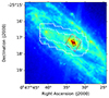 |
Fig. 1. Photometric image from Spitzer/IRAC at λ = 8 μm in logscale. The white contours show observations from SOFIA/FIFI-LS (solid – [O I]146 μm and [C II]158 μm, dashed – [O III]88 μm, dotted – [O III]52 μm and [O I]63 μm), the two black boxes show apertures of Spitzer/IRS short- and long high modules. The red box shows the approximate footprint of the Herschel/PACS observations. |
The FIFI-LS data were reduced with the FIFI-LS standard data reduction pipeline (Vacca et al. 2020). The pipeline performs a flux calibration, and resamples the data onto a spatial grid of 1.5″ × 1.5″ and 3″ × 3″ (pipeline spaxels) in the blue and red channels, respectively. The transmission of the atmosphere and hence the observed line flux at a given wavelength depend mainly on the total upward atmospheric precipitable water vapour (PWV). Inflight PWV values are determined by targeting specific water vapour features which are used in the data reduction pipeline for atmospheric calibration purposes (see Fischer et al. 2021 and Iserlohe et al. 2021 for more details). For our [O III]52 μm, [O III]88 μm, [O I]146 μm, and [C II]158 μm observations, we used the data from the pipeline that is PWV calibrated. The [O I]63 μm lies in a wavelength regime that is contaminated with a telluric absorption feature and is therefore not used in this study.
Flux density errors in the data cubes are the propagated errors from the ramp fit of the readout of the detector, but do not include errors from flux calibration or the PWV correction (FIFI-LS team, private communication). We therefore estimated the statistical flux density uncertainty from the root-mean-square (RMS) error in the continuum region of each pipeline spaxel. Due to the small spectral coverage, the continuum is nearly constant and the RMS error is not amplified by a non-constant continuum. For the [O III]52 μm, [O III]88 μm, [O I]146 μm, and [C II]158 μm observations, we excluded spectral regions with the expected line position. Due to a strong absorption feature at 51.7 μm, the flux density < 51.8 μm was also not included for the root-mean-square calculation (see Fig. 2 for an example spectrum and fit).
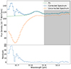 |
Fig. 2. Spectra of the pipeline spaxel (1.5″ × 1.5″) located toward the nucleus. The orange spectrum shows the observed spectrum (including errors from the ramp fit) without correction for atmospheric transmission. The telluric absorption feature at 51.7 μm can clearly be seen in the continuum. The blue spectrum shows the pipeline-corrected spectrum, including the errors determined as described in Sect. 2.1. The grey area shows the spectral region used to calculate flux density uncertainties. Green shows the best fit from the Monte Carlo method. |
To determine the line fluxes and their statistical uncertainties in each pipeline spaxel, we used a Monte Carlo approach, varying the flux density within the normal-distributed flux density uncertainties in each spectralbin randomly over 500 steps. The spectrum obtained from this variation was fitted with a linear continuum and a Gaussian with variable mean, width, and amplitude (see Fig. 2). From the integral over the Gaussian component, we obtained the line flux in each step − giving a sample of 500 line fluxes in each pipeline spaxel, from which we calculated the mean and standard deviation, which are the line flux and line flux error, respectively. These procedures were applied to the spectra from all pipeline spaxels, yielding the line flux maps shown in Fig. 3.
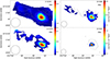 |
Fig. 3. Line flux maps from the SOFIA/FIFI-LS observations. Colour maps show the line flux in 10−17 W m−2 on a 3″ × 3″ (left column) and 1.5″ × 1.5″ (right column) grid, respectively. Pixels with a S/N smaller than 3 are masked. The black circles depict the aperture used to extract the spectrum from the nuclear region (Sect. 2.3.1). We also show contours from the fitted underlying continuum (grey). |
2.2. Additional data
2.2.1. Spitzer/IRS
We complement our data set with single slit spectra obtained with the Infrared Spectrograph (IRS, Houck et al. 2004) on board the Spitzer Space Telescope. Data are available at the Combined Atlas of Spitzer IRS Spectra (Lebouteiller et al. 2015, CASSIS1) under AOR key 9072640.
While the nuclear region of NGC 253 was observed with low- and high-resolution modules, we only use the short-high (SH) and long-high (LH) module observations, from 9.6−19.6 μm and 18.7−27.2 μm, because the low-resolution observations are saturated. Both high-resolution modules have a velocity resolution of Δv = 500 km s−1, comparable to the spectral resolution of our FIFI-LS observations. Slit sizes of the short- and long-wavelength module are different, 4.7″ × 11.3″ and 11.1″ × 22.3″, to better match the PSF size of each module.
CASSIS offers two reduction processes, the optimal extraction adapted to point-like sources, and full extraction adapted to extended sources. As the nucleus of NGC 253 is partly extended (see Sect. 2.3.2 and Fig. 6), we chose a full extraction procedure as this ensures we retrieve most of the flux of the source. The full extraction accounts for losses of flux density, and integrates the flux density over the full slit size. Although the nucleus of NGC 253 is not uniformly extended over the whole slit, which would be the ideal application for the full extraction, this process yields better results than optimal extraction.
For each emission line in the IRS spectrum, we fitted a Gaussian line profile and a polynomial of order 0–4 for the underlying continuum using lmfit. From the line fits, we obtained the line flux and line flux errors. In cases where several emission lines were close together, we fitted the continuum and all lines simultaneously. The high order for the continuum is necessary to account for the several broad emission and absorption features from, for instance, polycyclic aromatic hydrocarbons and silicates in the MIR. Line centroids are allowed to vary within 400 km s−1 with respect to the expected velocity from the source (see Table 1). The minimum line width is 300 km s−1, which is about the spectral resolution of IRS. Some lines are only weakly detected. We give an upper limit for the line flux if the obtained line flux from the fit is smaller than two times the RMS of the flux density of the continuum (in W m−2 μm−1) multiplied by the spectral resolution (in μm). In this case, the upper limit is given by two times the rms error of the continuum.
2.2.2. Herschel
We add to the FIFI-LS and Spitzer data observations with the Photodetector Array Camera and Spectrometer (PACS, Poglitsch et al. 2010) on board the Herschel Space Observatory2 (Pilbratt et al. 2010). We used PACSman v3.63 (Lebouteiller et al. 2012) for data reduction and analysis of the PACS spectral cubes. PACSman uses the rebinned data cubes from the PACS standard pipeline and fits a Gaussian emission line and a second-order polynomial for the underlying continuum in each of the 9.4″ × 9.4″ spaxels. PACSman provides a Monte Carlo-based method to determine the line flux errors in each spaxel. Similar to the procedure in Sect. 2.1, the flux density is varied within the Gaussian-distributed uncertainties in each of the 3000 steps. Each of the obtained spectra are fitted yielding a line flux in each spaxel. From the sample of 3000 line fluxes, we calculated the mean and standard deviation, ultimately providing the line flux and line flux error in one spaxel, respectively.
We obtained line flux maps and corresponding uncertainties for the [N III]57 μm, [O I]63 μm, [O III]88 μm, [N II]122 μm, [O I]146 μm, and [C II]158 μm transitions. See Fig. 4 for the observed spectra from the central 3 × 3 spaxels of the field-integral unit (cf. Sect. 2.3.3).
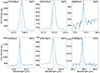 |
Fig. 4. Spectra of the nuclear region observed with the Herschel/PACS spectrometer. Only the spectrum of the central 3 × 3 spaxels is shown here (Sect. 2.3.3). The dashed line shows the redshift-corrected rest wavelength of the emission line. |
We finally complement our data set with Herschel/SPIRE-FTS observations. The SPIRE line fluxes from Pérez-Beaupuits et al. (2018) are already corrected for the semi-extended nuclear source (see Sect. 2.3), and therefore we do not reduce these observations and list only the results in Table 3. For details of the data reduction, see Pérez-Beaupuits et al. (2018).
2.3. Data homogenisation
We focus on emission from the nuclear source in this study, and therefore we have to determine the line fluxes and line flux errors arising only from the nucleus for each instrument.
2.3.1. SOFIA/FIFI-LS
The FIFI-LS line flux maps (Fig. 3) are oversampled, without knowledge of the correlation between the pipeline spaxels. In addition, the line flux maps are much more extended than only the nucleus and show emission from the bar and disc. To extract line fluxes and corresponding errors from only the nucleus, we proceeded as follows: we calculated an effective PSF size by fitting a Gaussian to the spatial profile of the nucleus for each emission line − the ideal PSF is broadened by the non-Nyquist sampling of the observations and the resample procedure in the pipeline. We resampled both the line flux maps (Fig. 3) and line flux error maps to a spatial grid of the effective PSF size. For the line flux error maps, we assumed that all pixels are fully correlated, meaning that the errors are cumulative. To get most of the line flux from the nucleus and avoid contamination from background (i.e., disc-) emission, we extracted the line flux and errors from the resampled maps using a circular aperture with a radius of two times the effective PSF FWHM, assuming that the pixels are uncorrelated. This means that errors add up quadratically. This procedure yields an upper limit for the line flux errors, because the assumption of the first step that all pixels are correlated is not entirely fulfilled. However, it is a good approximation as the errors are of the same order as the uncertainties from Herschel/PACS (see Table 3). The resulting spectra from this procedure are shown in Fig. 5.
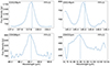 |
Fig. 5. Spectra from our FIFI-LS observations in the nuclear region of NGC 253. See Sect. 2.3.1 and Fig. 3 for details of the extraction aperture. |
All line fluxes and corresponding statistical errors from the FIFI-LS observations are listed in the second block of Table 3. The line fluxes listed are in good agreement with the values from Herschel/PACS as explained in Sect. 2.3.3. We compared the [O III]52 μm line flux with observations from the Kuiper Airborne Observatory (KAO), as this emission line was not observable with PACS. Compared to observations published by Carral et al. (1994), our value for [O III]52 μm emission is lower by ∼50%. However, the beam size of KAO at 52 μm is approximately eight times larger than that of SOFIA at that wavelength, so the KAO observations most likely include some background emission. To confirm that the KAO measurements of [O III]52 μm include diffuse emission, we extracted the spectrum from a 43″ aperture, which is the beam size of the KAO observations shown in Carral et al. (1994). Applying the same Monte Carlo method as in Sect. 2.1 we get a line flux of 107.7 ± 30.8 W m−2. This is in good agreement with the findings of Carral et al. (1994), who yielded a line flux of 90 ± 20 W m−2.
2.3.2. Spitzer/IRS
The spatial profile of the nuclear source is not point-like, but slightly extended, as can be seen from the cross-dispersion direction of the IRS LH slit (see Fig. 6). From the comparison of the observed spread and the ideal PSF, we get a spatial extent of the nucleus of 6.68″, corresponding to 113.6 pc under the assumed distance of 3.5 Mpc (see Table 1). This is in good agreement with the 6″ from [Ne II]13 μm observations by Engelbracht et al. (1998). We assume that the source size is the same for all MIR and FIR observations.
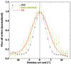 |
Fig. 6. Spatial profiles from the cross-dispersion direction of the LH module of IRS (see Lebouteiller et al. 2015, for details). Black shows the model PSF from observations of several point sources. Green diamonds show the spatial profile of NGC 253 in the observations, red is a Gaussian fit with a free FWHM. From the fit, we obtained a broadening of the PSF of 6.68″. |
As the spatial extent of the source is of the order of the size of the SH aperture size, the flux density in the SH observations is naturally underestimated due to a loss of flux outside the aperture. This leads to an offset between the continuum flux density of both SH and LH modules. To account for any lost flux density in the smaller SH aperture, we stitched the overlapping continua of both modules. We fit the spectrum of both modules in the overlapping continuum region (∼18.7−19.6 μm) linearly. From the fit we get an offset of the two continua of 1.55, and therefore we scale the SH spectrum by a factor of 1.55. We assume that the continuum and line emission arise from the same region, which is valid because the MIR continuum emission is mostly from hot dust in H II regions. We used broad band photometric images from the Midcourse Space Experiment (MSX3) at λ = 12.13 μm, 14.65 μm, and 21.3 μm to assert that no wavelength-dependent scaling is necessary. The more recent WISE observations are saturated and therefore cannot be used to verify the scaling. The continuum of the IRS spectra agrees within ∼10% with all three MSX bands, and therefore no wavelength-dependent scaling is needed. The resulting spectrum and MSX measurements are shown in Fig. 7. Footprints of SH and LH observations can be seen in Fig. 1.
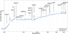 |
Fig. 7. Spitzer/IRS spectrum (blue) and MSX broadband flux density measurements (red dots) of the nuclear region (11.1″ × 22.3″) of NGC 253. Detected emission lines in the Spitzer spectrum are labelled accordingly. MSX filter bandwidths are indicated in dashed lines. |
Line fluxes from both modules and other parameters of the observed lines are listed in Table 3. Our values are in good agreement with values from Bernard-Salas et al. (2009) who used the same data set.
2.3.3. Herschel/PACS
To get the integrated line flux from the nuclear source from the PACS line flux maps created in Sect. 2.2.2, we summed up the line flux from the central 3 × 3 spaxels (28.2″ × 28.2″) to limit background emission and noise from the weakly illuminated outer pixels, and to only extract the nuclear source flux. A comparison of our line fluxes with Pérez-Beaupuits et al. (2018) shows consistency within the error bars for all lines except [C II]158 μm, which is ∼20% weaker in our case. However, when comparing the [C II]158 μm line flux from all 5 × 5 spaxels, the results are again in good agreement. The large difference between these two values is due to a significant contribution of [C II]158 μm from the underlying disc. Line fluxes and errors of the brightest fine-structure lines observed with PACS are listed in Table 3.
3. Analysis
We used ratios of our MIR and FIR integrated line fluxes to determine parameters of the ISM. These fine-structure lines are in most cases not affected by extinction or self-absorption. Furthermore, when studying line ratios from the same species (e.g., [O III]52/88 μm) the ratio is independent of the ionic abundance of O2+. This is particularly important, because the elemental abundances are uncertain for NGC 253.
3.1. Optical depth
Luminous IR objects tend to be highly extincted sources, making it sometimes necessary to correct for extinction even at MIR wavelengths, particularly for AV ≥ 10 mag (Armus et al. 2007). We therefore have to correct the MIR line fluxes for extinction or make sure that such correction is not needed for our modelling approach. The optical depth determinations for the nuclear region in NGC 253 vary within the literature from AV = 5.5 mag (Pérez-Beaupuits et al. 2018, from dust SED fit), to AV = 14.0 mag (Rieke et al. 1980, from Brα/Brγ), and up to AV = 19.1 mag (Engelbracht et al. 1998, from [Fe II]), depending on the tracers.
To determine the optical depth of the nuclear region of NGC 253, we used the SED fitting tool MAGPHYS (da Cunha et al. 2008). Based on a set of photometric observations between the UV and FIR range as input, MAGPHYS fits the SED of a galaxy. MAGPHYS varies different parameters for the stellar emission (e.g., SFR and initial mass function), and dust attenuation and emission (e.g. optical depth and dust mass) and fits the SED by minimising the χ2 between observations and modelled SED. It is not possible to fix any of the parameters, all variables are free. As input data, we used photometric observations from the archives of different observatories, covering the spectral range from the UV to the FIR. We used data from GALEX in the far-UV (FUV) and near-UV (NUV) bands, 2MASS in the J, H, and Ks bands, Spitzer/IRAC bands 1−4 and Herschel/PACS bands 70, 100, and 160 μm. The MSX filters are not available in MAGPHYS and are therefore not used to model the SED. Details about the different photometric bands are reported in Table 4.
We obtained the flux density maps from the respective archives of the different observatories. To get only the flux density from the nucleus, we convolved the source size of 6.68″ (see Fig. 6) with the resolution of the different observatories at the given wavelength and extracted the flux density from an aperture of the resulting diameter. We assume that the nuclear emission is dominant in this region and that emission from other structures, such as the bar, is negligible. The obtained measurements are listed in Table 4 and shown in Fig. 8. Using these flux densities as input, MAGPHYS determines the best-fitting SED and returns the fitted parameters. From the fit, we obtained a total IR luminosity LTIR = 1.37 × 10¹⁰ L⊙. We also used the prescription given in Galametz et al. (2013; see their Eq. (7) and Table 3) to calculate LTIR from FIR data only. From this prescription – using the Herschel/PACS photometric data only – we obtain LTIR = (9.2 ± 0.4)×109 L⊙, which is in good agreement with the result from MAGPHYS. MAGPHYS also returns the optical depth, which is AV = 4.35 mag. This again is in good agreement with the findings of a recent study (Pérez-Beaupuits et al. 2018) who obtained AV = 5.5 ± 2.5 mag from the 100 μm dust continuum emission. The fitted SED is shown in Fig. 8.
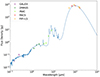 |
Fig. 8. Broadband measurements from GALEX, 2MASS, Spitzer/IRAC, and Herschel/PACS observations and the resulting SED fit from MAGPHYS (blue). We also include the continuum from the SOFIA/FIFI-LS observations (Sect. 2.1) which are in good agreement with the fitted SED. |
Using the models from Weingartner & Draine (2001) with RV = 3.1 and the optical depth we obtained (AV = 4.35 mag) we calculated optical depths at other wavelengths. We yield an optical depth at λ = 20 μm of A20 μm = 0.13 mag, which translates into an extinction correction for the line fluxes of ∼12%. The wavelengths of the emission lines used for the line flux ratios are close, and therefore the extinction affects the line ratios even less. In the case of the ([Ne II]13 μm + [Ne III] 16μm)/Hα, the extinction correction is 3.5%. We find that the extinction correction has little effect on the set of lines used in our study.
3.2. Ionised gas density
Densities of the nuclear region of NGC 253 are reported in the literature to range from ∼4.3 × 102 cm−3 (Carral et al. 1994, from [O III]) up to 5 × 103 cm−3 (Engelbracht et al. 1998, from [Fe II]) for the ionised gas. The results depend on the tracers used, which could, in principle, apply to different regions within the observing beam or could be associated with different regions due to poorer spatial resolution.
Several observed line flux ratios are sensitive to the density of the H II region. Well-known examples are the [O III]52 μm/[O III]88 μm and [N II]122 μm/[N II]205 μm ratios (e.g., Carral et al. 1994; Oberst et al. 2011; Herrera-Camus et al. 2016). Additionally, the MIR line flux ratios [Ne III]16 μm/[Ne III]36 μm, [Ne V]14 μm/[Ne V]24 μm, and [S III]19 μm/[S III]33 μm are excellent tracers for the density of the ionised gas because they are independent of the ionic abundance and are weakly dependent on the electron temperature. These line flux ratios are not only ideal tracers of the density – because of their different critical densities (see Table 3) –, but they potentially also trace different regions of the ionised ISM, as shown in Fig. 9. Owing to the critical densities, the line flux ratio [N II]122 μm/[N II]205 μm is a good tracer for the diffuse outskirts of [H II] regions (Oberst et al. 2011), the ratios [S III]19 μm/[S III]33 μm and [Ne III]16 μm/[Ne III]36 μm trace a higher density phase. Furthermore, the [Ne V]14 μm/[Ne V]24 μm traces the gas phase, the conditions of which are dominated by the AGN because Ne4+ is not produced by stars but by the accretion disc from an AGN or fast radiative shocks (Izotov et al. 2012).
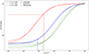 |
Fig. 9. Density dependence (logscale) of the [O III]52 μm/[O III]88 μm, [N II]122 μm/[N II]205 μm, and [S III]19 μm/[S III]33 μm line flux ratios for different temperatures. The various line flux ratios are sensitive to different density regimes. The results from [N II]122 μm/[N II]205 μm and [S III]19 μm/[S III]33 μm are indicated in red and green dots, respectively, and for [O III]52 μm/[O III]88 μm we show the upper density limit (blue dots). |
We used a Monte Carlo method to obtain a density from these line flux ratios and also to propagate uncertainties. With the Monte Carlo method we were also able to investigate whether or not the influence of the electron temperature is indeed negligible.
To determine the hydrogen density, we used the Python package PyNeb (Luridiana et al. 2013). PyNeb calculates the density of the ionised gas, if two density-dependent emission lines and the temperature of the gas are provided, by solving the equilibrium equations of the n-level atom and determining the level populations. We assumed a normal distribution for the line fluxes, where the mean of the distribution is given by the line flux and the standard deviation corresponds to the statistical uncertainties given in Table 3. For the calculations, the temperature is uniformly distributed between 7000 K and 13 000 K, which are typical values for the gas in [H II] regions (Osterbrock & Ferland 2006). In each of the 105 steps, a temperature and line flux for each of the ionised species of a pair of lines were randomly picked and a density was calculated. The results of these calculations are shown in the left panel of Fig. 10 for the [S III]19 μm/[S III]33 μm line flux ratio.
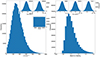 |
Fig. 10. Results from the Monte Carlo simulation to derive the hydrogen density (Sect. 3.2) and the Ne/H abundance ratio (Sect. 3.3). Left: main plot showing the derived density in 10 cm−3 bins. Inset plots show histograms of the randomly picked temperature (uniform distribution, 1000 K bins), and integrated line fluxes for [S III]19 μm and [S III]33 μm. Right: inset plots again showing histograms of the randomly picked integrated line fluxes of [Ne II]13 μm, [Ne III]16 μm, and Hu α. From the line fluxes, temperature, and density, we obtained the Ne/H abundance ratio in solar units, which is shown in the main plot (0.1 bins). |
We applied this Monte Carlo method to all line flux ratios listed above. However, from the [Ne III]16 μm/[Ne III]36 μm and [Ne V]14 μm/[Ne V]24 μm we did not obtain any results as these line flux ratios did not allow PyNeb to solve the level populations. We derived the densities listed in Table 5 from the line flux ratios.
The obtained densities from [S III]19 μm/[S III]33 μm and [N II]122 μm/[N II]205 μm are in good agreement with each other despite the different critical densities. In contrast, the [O III]52 μm/[O III]88 μm is lower by a factor of 2. The density obtained from the ratio [O III]52 μm/[O III]88 μm lies within a range where the line flux ratio is not sensitive to the density, and therefore we only give an upper limit for the density. For the latter line flux ratio, we used both lines from the FIFI-LS observations to reduce systematic effects.
The densities derived from all line flux ratios are significantly lower than results from other studies (e.g., Engelbracht et al. 1998). For the [N II] line flux ratio, this is most likely due to the low critical densities of both transitions. Both the [N II]122 μm and [N II]205 μm lines are therefore associated with diffuse, low-density regions and do not trace high-density regimes. The [S III] line flux ratio traces higher density regions (see Fig. 9), but the S+ ion has a higher ionisation potential (see Table 3) compared to, for example, Fe+. Nevertheless, Fe+ was used in Engelbracht et al. (1998). The different excitation potential and critical density of the species could explain the discrepancy between the results of our study and this latter. The ratio [O III]52 μm/[O III]88 μm was also used by Carral et al. (1994). The difference between the results of Carral et al. (1994) and those presented here is most likely due to the different sizes of observing beams, leading to a higher [O III]52 μm line flux and, hence, to a higher density, as discussed in Sect. 2.3.1. We conclude that, although all densities are in moderate agreement with each other, to appropriately model the ionised gas in the nuclear region at least a two-phase model would be needed, because of the different critical densities and ionisation potentials of the used species.
3.3. Chemical composition
The determinations of metallicity in the nuclear region of NGC 253 vary widely within the literature. The metallicity ranges from ∼0.5 Z⊙ (Carral et al. 1994; Ptak et al. 1997), to ≲1 Z⊙ (Engelbracht et al. 1998), and up to ≲1.5 Z⊙ (Webster & Smith 1983).
We calculated the metallicity with the available emission lines self-consistently. The [Ne II]13 μm, [Ne III]16 μm, and Hu α together provide excellent constraints for this purpose, and we can use the ([Ne II]13 μm + [Ne III]16 μm)/Hu α line flux ratio, which is sensitive to the Ne/H abundance in the gas (Bernard Salas et al. 2001; Lebouteiller et al. 2008). The lines arise from the ionised gas and Ne is not depleted on dust grains; the Ne/H is therefore an ideal tracer for the metallicity of the gas.
To calculate the Ne/H abundance ratio, we again used the Python tool PyNeb. For a given temperature T, density n, and line flux ratio [Ne II]13 μm/Hu α, PyNeb predicts the Ne+/H abundance ratio by solving the equilibrium equations and level populations for the Ne and H atom. The procedure is the same for the line flux ratio [Ne III]16 μm/Hu α, yielding the abundance ratio Ne2+/H. We assumed that Ne+ and Ne2+ are the dominant ionisation stages, that is Ne/H = Ne+/H + Ne2+/H. Under this assumption, we can use the densities derived in Sect. 3.2.
Again, we used the Monte Carlo method to propagate uncertainties in the derived Ne/H abundance ratio. We calculated the Ne/H abundance ratio assuming the different densities we obtained from the [S III], [N II], and [S III] line flux ratios in Sect. 3.2. To do so, we extended our Monte Carlo approach from Sect. 3.2. After calculating the density from the randomly drawn line fluxes (e.g., for [S III]19 μm and [S III]33 μm), line fluxes for [Ne II]13 μm, [Ne III]16 μm, and Hu α were drawn; the distributions for these lines are again normal distributions. With these three emission lines, as well as the temperature and density from the first step (Sect. 3.2), we calculated the Ne/H abundance ratio for 105 steps. From this sample, we calculated the mean and standard deviation.
The results are shown in the right panels of Fig. 10. We obtain a Ne/H abundance ratio of nearly solar value, [Ne/H][O III = 1.08 ± 0.41, [Ne/H]N II = 1.00 ± 0.24, and [Ne/H][S III] = 1.00 ± 0.24. The similar results suggest that the density does not seem to play a major role in the metallicity determination in the examined density regimes. From the Ne/H abundance, we use equations given by Izotov & Thuan (1999), Izotov et al. (2006), and Nicholls et al. (2017), who studied elemental abundances in galaxies to deduce abundances for C, N, O, Si, S, and Fe. The abundances of these elements are given in Table 6.
Gas-phase elemental abundances relative to the hydrogen abundance for most of the species that were observed.
As discussed by Madden et al. (2020) for example, the metallicity is of great importance for determining the CO-to-H2 conversion factor αCO. Using the results from previous studies, αCO (in M⊙ pc−2(K km s−1)−1) ranges from ∼1 up to ∼40, covering more than 1.5 orders of magnitude. From our obtained metallicity and Eq. (6) in Madden et al. (2020), we yield a more accurate αCO of  .
.
4. Summary and outlook
In this first of a series of papers, we present a wealth of MIR and FIR data of the nuclear region of the starburst galaxy NGC 253 from the SOFIA, Herschel, and Spitzer telescopes. We describe the data-reduction steps for each observatory and note caveats that appeared during these processes. The full list of observed lines, the line fluxes, and errors from the nuclear region are listed in Table 3, and the extended line flux maps we obtained from SOFIA/FIFI-LS observations are shown in Fig. 3.
Furthermore, we used the obtained line fluxes to derive fundamental parameters of the local ISM, such as density n, metallicity Z, and optical depth AV. We show that for our observed MIR emission lines, no extinction correction is needed. We used the line flux ratios of [S III], [S III], and [N II], which are almost independent of the local temperature and mostly depend on the gas density or, more precisely, on the local density of electrons, which are the main collisional partners to excite these states. We conclude that there are at least two ionised gas phases in the central region of this galaxy. From the calculated density and assumed temperature, we used the line flux ratio of ([Ne II]13 μm + [Ne III]16 μm)/Hu α – which is an ideal tracer for the Ne/H abundance – to calculate the local metallicity, for which we obtain solar value.
In a forthcoming paper, we will use all observed lines to create a more sophisticated multi-phase model using MULTIGRIS, a Bayesian approach to determine the probability density distribution within a set of Cloudy models (Lebouteiller & Ramambason 2022; Ramambason et al. 2022) of ISM parameters such as density, intensity of radiation field, and age of the starburst.
Obs. ID 1342210652, 1342212531
Available at https://irsa.ipac.caltech.edu/data/MSX/
Acknowledgments
The authors thank the anonymous referee for useful comments that improved the quality and clarity of the paper. SOFIA, the Stratospheric Observatory For Infrared Astronomy, is a joint project of the Deutsche Raumfahrtagentur im Deutschen Zentrum für Luft- und Raumfahrt e.V. (German Space Agency at DLR, grant: FKZ 50OK2002) and the National Aeronautics and Space Administration (NASA). It is funded on behalf of the German Space Agency at DLR by the Federal Ministry for Economic Affairs and Climate Action based on legislation by the German Parliament, the state of Baden-Württemberg and the University of Stuttgart. Scientific operation for Germany is coordinated by the Deutsches SOFIA Institut (DSI) at the University of Stuttgart. Software: Astropy (Astropy Collaboration 2013, 2018), Photutils (Bradley et al. 2021), Matplotlib (Hunter 2007), NumPy (Harris et al. 2020), SciPy (Virtanen et al. 2020)
References
- Armus, L., Charmandaris, V., Bernard-Salas, J., et al. 2007, ApJ, 656, 148 [NASA ADS] [CrossRef] [Google Scholar]
- Astropy Collaboration (Robitaille, T. P., et al. 2013, A&A, 558, A33 [NASA ADS] [CrossRef] [EDP Sciences] [Google Scholar]
- Astropy Collaboration (Price-Whelan, A. M., et al.) 2018, AJ, 156, 123 [Google Scholar]
- Bernard Salas, J., Pottasch, S. R., Beintema, D. A., & Wesselius, P. R. 2001, A&A, 367, 949 [NASA ADS] [CrossRef] [EDP Sciences] [Google Scholar]
- Bernard-Salas, J., Spoon, H. W. W., Charmandaris, V., et al. 2009, ApJS, 184, 230 [Google Scholar]
- Bolatto, A. D., Warren, S. R., Leroy, A. K., et al. 2013a, Nature, 499, 450 [Google Scholar]
- Bolatto, A. D., Wolfire, M., & Leroy, A. K. 2013b, ARA&A, 51, 207 [CrossRef] [Google Scholar]
- Bradley, L., Sipőcz, B., Robitaille, T., et al. 2021, https://doi.org/10.5281/zenodo.596036 [Google Scholar]
- Carral, P., Hollenbach, D. J., Lord, S. D., et al. 1994, ApJ, 423, 223 [NASA ADS] [CrossRef] [Google Scholar]
- Colditz, S., Beckmann, S., Bryant, A., et al. 2018, J. Astron. Instrum., 7, 1840004 [Google Scholar]
- Cormier, D., Lebouteiller, V., Madden, S. C., et al. 2012, A&A, 548, A20 [NASA ADS] [CrossRef] [EDP Sciences] [Google Scholar]
- da Cunha, E., Charlot, S., & Elbaz, D. 2008, MNRAS, 388, 1595 [Google Scholar]
- Draine, B. T. 2011, Physics of the Interstellar and Intergalactic Medium (Princeton: Princeton University Press) [Google Scholar]
- Engelbracht, C. W., Rieke, M. J., Rieke, G. H., Kelly, D. M., & Achtermann, J. M. 1998, ApJ, 505, 639 [NASA ADS] [CrossRef] [Google Scholar]
- Ferland, G. J., Chatzikos, M., Guzmán, F., et al. 2017, Rev. Mex. Astron., 53, 385 [NASA ADS] [Google Scholar]
- Fernández-Ontiveros, J. A., Prieto, M. A., & Acosta-Pulido, J. A. 2009, MNRAS, 392, L16 [CrossRef] [Google Scholar]
- Fernández-Ontiveros, J. A., Spinoglio, L., Pereira-Santaella, M., et al. 2016, ApJS, 226, 19 [CrossRef] [Google Scholar]
- Fischer, C., Bryant, A., Beckmann, S., et al. 2016, Proc. SPIE, 9910, 991027 [NASA ADS] [CrossRef] [Google Scholar]
- Fischer, C., Beckmann, S., Bryant, A., et al. 2018, J. Astron. Instrum., 7, 1840003 [Google Scholar]
- Fischer, C., Iserlohe, C., Vacca, W., et al. 2021, PASP, 133, 055001 [NASA ADS] [CrossRef] [Google Scholar]
- Galametz, M., Kennicutt, R. C., Calzetti, D., et al. 2013, MNRAS, 431, 1956 [NASA ADS] [CrossRef] [Google Scholar]
- Giveon, U., Sternberg, A., Lutz, D., Feuchtgruber, H., & Pauldrach, A. W. A. 2002, ApJ, 566, 880 [NASA ADS] [CrossRef] [Google Scholar]
- Günthardt, G. I., Agüero, M. P., Camperi, J. A., et al. 2015, AJ, 150, 139 [CrossRef] [Google Scholar]
- Harris, C. R., Millman, K. J., van der Walt, S. J., et al. 2020, Nature, 585, 357 [NASA ADS] [CrossRef] [Google Scholar]
- Herrera-Camus, R., Bolatto, A., Smith, J. D., et al. 2016, ApJ, 826, 175 [Google Scholar]
- Houck, J. R., Roellig, T. L., van Cleve, J., et al. 2004, ApJS, 154, 18 [NASA ADS] [CrossRef] [Google Scholar]
- Hunter, J. D. 2007, Comput. Sci. Eng., 9, 90 [NASA ADS] [CrossRef] [Google Scholar]
- Iodice, E., Arnaboldi, M., Rejkuba, M., et al. 2014, A&A, 567, A86 [NASA ADS] [CrossRef] [EDP Sciences] [Google Scholar]
- Iserlohe, C., Fischer, C., Vacca, W. D., et al. 2021, PASP, 133, 055002 [NASA ADS] [CrossRef] [Google Scholar]
- Izotov, Y. I., & Thuan, T. X. 1999, ApJ, 511, 639 [NASA ADS] [CrossRef] [Google Scholar]
- Izotov, Y. I., Stasińska, G., Meynet, G., Guseva, N. G., & Thuan, T. X. 2006, A&A, 448, 955 [CrossRef] [EDP Sciences] [Google Scholar]
- Izotov, Y. I., Thuan, T. X., & Privon, G. 2012, MNRAS, 427, 1229 [NASA ADS] [CrossRef] [Google Scholar]
- Kaufman, M. J., Wolfire, M. G., & Hollenbach, D. J. 2006, ApJ, 644, 283 [Google Scholar]
- Klein, R., Beckmann, S., Bryant, A., et al. 2014, Proc. SPIE, 9147, 91472X [NASA ADS] [CrossRef] [Google Scholar]
- Kramida, A., Ralchenko, Yu., Reader, J., & NIST ASD Team 2020, NIST Atomic Spectra Database (ver. 5.8), https://physics.nist.gov/asd [Google Scholar]
- Krips, M., Martín, S., Sakamoto, K., et al. 2016, A&A, 592, L3 [NASA ADS] [CrossRef] [EDP Sciences] [Google Scholar]
- Lebouteiller, V., & Ramambason, L. 2022, A&A, in press, https://doi.org/10.1051/0004-6361/202243865 [Google Scholar]
- Lebouteiller, V., Bernard-Salas, J., Brandl, B., et al. 2008, ApJ, 680, 398 [NASA ADS] [CrossRef] [Google Scholar]
- Lebouteiller, V., Cormier, D., Madden, S. C., et al. 2012, A&A, 548, A91 [NASA ADS] [CrossRef] [EDP Sciences] [Google Scholar]
- Lebouteiller, V., Barry, D. J., Goes, C., et al. 2015, ApJS, 218, 21 [Google Scholar]
- Leroy, A. K., Bolatto, A. D., Ostriker, E. C., et al. 2015, ApJ, 801, 25 [NASA ADS] [CrossRef] [Google Scholar]
- Luridiana, V., Morisset, C., & Shaw, R. A. 2013, Astrophysics Source Code Library [record ascl:1304.021] [Google Scholar]
- Madden, S. C., Cormier, D., Hony, S., et al. 2020, A&A, 643, A141 [NASA ADS] [CrossRef] [EDP Sciences] [Google Scholar]
- Malhotra, S., Kaufman, M. J., Hollenbach, D., et al. 2001, ApJ, 561, 766 [Google Scholar]
- Martín, S., Mangum, J. G., Harada, N., et al. 2021, A&A, 656, A46 [NASA ADS] [CrossRef] [EDP Sciences] [Google Scholar]
- Meijerink, R., Spaans, M., & Israel, F. P. 2007, A&A, 461, 793 [NASA ADS] [CrossRef] [EDP Sciences] [Google Scholar]
- Müller-Sánchez, F., González-Martín, O., Fernández-Ontiveros, J. A., Acosta-Pulido, J. A., & Prieto, M. A. 2010, ApJ, 716, 1166 [CrossRef] [Google Scholar]
- Nicholls, D. C., Sutherland, R. S., Dopita, M. A., Kewley, L. J., & Groves, B. A. 2017, MNRAS, 466, 4403 [Google Scholar]
- Oberst, T. E., Parshley, S. C., Nikola, T., et al. 2011, ApJ, 739, 100 [NASA ADS] [CrossRef] [Google Scholar]
- Osterbrock, D. E., & Ferland, G. J. 2006, Astrophysics of Gaseous Nebulae and Active Galactic Nuclei (University Science Books) [Google Scholar]
- Pence, W. D. 1981, ApJ, 247, 473 [NASA ADS] [CrossRef] [Google Scholar]
- Pérez-Beaupuits, J. P., Güsten, R., Harris, A., et al. 2018, ApJ, 860, 23 [Google Scholar]
- Pérez-Montero, E., Contini, T., Lamareille, F., et al. 2013, A&A, 549, A25 [NASA ADS] [CrossRef] [EDP Sciences] [Google Scholar]
- Pilbratt, G. L., Riedinger, J. R., Passvogel, T., et al. 2010, A&A, 518, L1 [NASA ADS] [CrossRef] [EDP Sciences] [Google Scholar]
- Poglitsch, A., Waelkens, C., Geis, N., et al. 2010, A&A, 518, L2 [NASA ADS] [CrossRef] [EDP Sciences] [Google Scholar]
- Ptak, A., Serlemitsos, P., Yaqoob, T., Mushotzky, R., & Tsuru, T. 1997, AJ, 113, 1286 [NASA ADS] [CrossRef] [Google Scholar]
- Radovich, M., Kahanpää, J., & Lemke, D. 2001, A&A, 377, 73 [NASA ADS] [CrossRef] [EDP Sciences] [Google Scholar]
- Ramambason, L., Lebouteiller, V., Bik, A., et al. 2022, A&A, in press, https://doi.org/10.1051/0004-6361/202243866 [Google Scholar]
- Rekola, R., Richer, M. G., McCall, M. L., et al. 2005, MNRAS, 361, 330 [NASA ADS] [CrossRef] [Google Scholar]
- Rieke, G. H., Lebofsky, M. J., Thompson, R. I., Low, F. J., & Tokunaga, A. T. 1980, ApJ, 238, 24 [NASA ADS] [CrossRef] [Google Scholar]
- Rosenberg, M. J. F., van der Werf, P. P., & Israel, F. P. 2013, A&A, 550, A12 [NASA ADS] [CrossRef] [EDP Sciences] [Google Scholar]
- Sloan, G. C., Herter, T. L., Charmandaris, V., et al. 2015, AJ, 149, 11 [NASA ADS] [CrossRef] [Google Scholar]
- Spinoglio, L., Fernández-Ontiveros, J. A., Malkan, M. A., et al. 2022, ApJ, 926, 55 [NASA ADS] [CrossRef] [Google Scholar]
- Vacca, W., Clarke, M., Perera, D., Fadda, D., & Holt, J. 2020, in ASP Conf. Ser., eds. R. Pizzo, E. R. Deul, J. D. Mol, J. de Plaa, & H. Verkouter, 527, 547 [NASA ADS] [Google Scholar]
- Virtanen, P., Gommers, R., Oliphant, T. E., et al. 2020, Nat. Methods, 17, 261 [Google Scholar]
- Vogler, A., & Pietsch, W. 1999, A&A, 342, 101 [NASA ADS] [Google Scholar]
- Walter, F., Bolatto, A. D., Leroy, A. K., et al. 2017, ApJ, 835, 265 [NASA ADS] [CrossRef] [Google Scholar]
- Webster, B. L., & Smith, M. G. 1983, MNRAS, 204, 743 [NASA ADS] [Google Scholar]
- Weingartner, J. C., & Draine, B. T. 2001, ApJ, 548, 296 [Google Scholar]
- Young, E. T., Becklin, E. E., Marcum, P. M., et al. 2012, ApJ, 749, L17 [NASA ADS] [CrossRef] [Google Scholar]
All Tables
Gas-phase elemental abundances relative to the hydrogen abundance for most of the species that were observed.
All Figures
|
Fig. 1. Photometric image from Spitzer/IRAC at λ = 8 μm in logscale. The white contours show observations from SOFIA/FIFI-LS (solid – [O I]146 μm and [C II]158 μm, dashed – [O III]88 μm, dotted – [O III]52 μm and [O I]63 μm), the two black boxes show apertures of Spitzer/IRS short- and long high modules. The red box shows the approximate footprint of the Herschel/PACS observations. |
| In the text | |
|
Fig. 2. Spectra of the pipeline spaxel (1.5″ × 1.5″) located toward the nucleus. The orange spectrum shows the observed spectrum (including errors from the ramp fit) without correction for atmospheric transmission. The telluric absorption feature at 51.7 μm can clearly be seen in the continuum. The blue spectrum shows the pipeline-corrected spectrum, including the errors determined as described in Sect. 2.1. The grey area shows the spectral region used to calculate flux density uncertainties. Green shows the best fit from the Monte Carlo method. |
| In the text | |
|
Fig. 3. Line flux maps from the SOFIA/FIFI-LS observations. Colour maps show the line flux in 10−17 W m−2 on a 3″ × 3″ (left column) and 1.5″ × 1.5″ (right column) grid, respectively. Pixels with a S/N smaller than 3 are masked. The black circles depict the aperture used to extract the spectrum from the nuclear region (Sect. 2.3.1). We also show contours from the fitted underlying continuum (grey). |
| In the text | |
|
Fig. 4. Spectra of the nuclear region observed with the Herschel/PACS spectrometer. Only the spectrum of the central 3 × 3 spaxels is shown here (Sect. 2.3.3). The dashed line shows the redshift-corrected rest wavelength of the emission line. |
| In the text | |
|
Fig. 5. Spectra from our FIFI-LS observations in the nuclear region of NGC 253. See Sect. 2.3.1 and Fig. 3 for details of the extraction aperture. |
| In the text | |
|
Fig. 6. Spatial profiles from the cross-dispersion direction of the LH module of IRS (see Lebouteiller et al. 2015, for details). Black shows the model PSF from observations of several point sources. Green diamonds show the spatial profile of NGC 253 in the observations, red is a Gaussian fit with a free FWHM. From the fit, we obtained a broadening of the PSF of 6.68″. |
| In the text | |
|
Fig. 7. Spitzer/IRS spectrum (blue) and MSX broadband flux density measurements (red dots) of the nuclear region (11.1″ × 22.3″) of NGC 253. Detected emission lines in the Spitzer spectrum are labelled accordingly. MSX filter bandwidths are indicated in dashed lines. |
| In the text | |
|
Fig. 8. Broadband measurements from GALEX, 2MASS, Spitzer/IRAC, and Herschel/PACS observations and the resulting SED fit from MAGPHYS (blue). We also include the continuum from the SOFIA/FIFI-LS observations (Sect. 2.1) which are in good agreement with the fitted SED. |
| In the text | |
|
Fig. 9. Density dependence (logscale) of the [O III]52 μm/[O III]88 μm, [N II]122 μm/[N II]205 μm, and [S III]19 μm/[S III]33 μm line flux ratios for different temperatures. The various line flux ratios are sensitive to different density regimes. The results from [N II]122 μm/[N II]205 μm and [S III]19 μm/[S III]33 μm are indicated in red and green dots, respectively, and for [O III]52 μm/[O III]88 μm we show the upper density limit (blue dots). |
| In the text | |
|
Fig. 10. Results from the Monte Carlo simulation to derive the hydrogen density (Sect. 3.2) and the Ne/H abundance ratio (Sect. 3.3). Left: main plot showing the derived density in 10 cm−3 bins. Inset plots show histograms of the randomly picked temperature (uniform distribution, 1000 K bins), and integrated line fluxes for [S III]19 μm and [S III]33 μm. Right: inset plots again showing histograms of the randomly picked integrated line fluxes of [Ne II]13 μm, [Ne III]16 μm, and Hu α. From the line fluxes, temperature, and density, we obtained the Ne/H abundance ratio in solar units, which is shown in the main plot (0.1 bins). |
| In the text | |
Current usage metrics show cumulative count of Article Views (full-text article views including HTML views, PDF and ePub downloads, according to the available data) and Abstracts Views on Vision4Press platform.
Data correspond to usage on the plateform after 2015. The current usage metrics is available 48-96 hours after online publication and is updated daily on week days.
Initial download of the metrics may take a while.