| Issue |
A&A
Volume 680, December 2023
|
|
|---|---|---|
| Article Number | A55 | |
| Number of page(s) | 14 | |
| Section | Extragalactic astronomy | |
| DOI | https://doi.org/10.1051/0004-6361/202347557 | |
| Published online | 12 December 2023 | |
Infrared view of the multiphase ISM in NGC 253
II. Modelling the ionised and neutral atomic gas
1
Deutsches SOFIA Institut, University of Stuttgart, Pfaffenwaldring 29, 70569 Stuttgart, Germany
e-mail: This email address is being protected from spambots. You need JavaScript enabled to view it.
2
AIM, CEA, CNRS, Université Paris-Saclay, Université Paris-Diderot, Sorbonne Paris-Cité, 91191 Gif-sur-Yvette, France
3
Max-Planck-Institut für Radioastronomie, Auf dem Hügel 69, 53121 Bonn, Germany
4
Centro de Astro-Ingeniería (AIUC), Pontificia Universidad Católica de Chile, Av. Vicuña Mackena 4860, Macul, Santiago, Chile
5
Institut für Theoretische Astrophysik, Zentrum für Astronomie, Universität Heidelberg, Albert-Ueberle-Str. 2, 69120 Heidelberg, Germany
6
Universidad Autonoma de Chile, Pedro de Valdivia 425, Providencia, Santiago de Chile, Chile
Received:
25
July
2023
Accepted:
29
September
2023
Abstract
Context. Multi-wavelength studies of galaxies and galactic nuclei allow us to build a relatively more complete picture of the interstellar medium (ISM), especially in the dusty regions of starburst galaxies. An understanding of the physical processes in nearby galaxies can assist in the study of more distant sources at higher redshifts that cannot be resolved.
Aims. We aimed to use observations presented in the first part of this series of papers to model the physical conditions of the ISM in the nuclear region of NGC 253, in order to obtain primary parameters such as gas densities and metallicities. From the model we created, we further calculated secondary parameters, such as gas masses of the different phases, and estimated the fraction of [C II]158 μ m from the different phases, which allowed us to probe the nuclear star formation rate.
Methods. To compare theory with our observations we used MULTIGRIS, a probabilistic tool that determines probabilities for certain ISM parameters from a grid of Cloudy models together with a set of spectroscopic lines.
Results. We find that the hypothetical active galactic nucleus within NGC 253 has only a minor impact, compared to the starburst, on the heating of the ISM, as probed by the observed lines. We characterise the ISM and obtain parameters such as a solar metallicity, a mean density of ∼230 cm−3, an ionisation parameter of log U ≈ −3, and an age of the nuclear cluster of ∼2 Myr. Furthermore, we estimate the masses of the ionised (3.8 × 10⁶ M⊙), neutral atomic (9.1 × 10⁶ M⊙), and molecular (2.0 × 10⁸ M⊙) gas phases as well as the dust mass (1.8 × 10⁶ M⊙) in the nucleus of NGC 253.
Key words: galaxies: ISM / galaxies: starburst
© The Authors 2023
 Open Access article, published by EDP Sciences, under the terms of the Creative Commons Attribution License (https://creativecommons.org/licenses/by/4.0), which permits unrestricted use, distribution, and reproduction in any medium, provided the original work is properly cited.
This article is published in open access under the Subscribe to Open model. This email address is being protected from spambots. You need JavaScript enabled to view it. to support open access publication.
1. Introduction
In the extreme environments of galactic nuclei, the various heating and cooling mechanisms at work within the interstellar medium (ISM) are notoriously entangled. Consequently, the physical conditions of the ISM are difficult to constrain. In particular, the heating mechanisms are strenuous to unravel, as they are typically and indirectly probed through specific corresponding cooling processes. Multi-wavelength observations and models, ideally with tracers sensitive to the different ISM phases, are therefore mandatory to link heating and cooling processes that regulate the matter cycle and star formation. Nearby galaxies, such as NGC 253 at a distance of 3.5 Mpc (Rekola et al. 2005), are ideal laboratories in which to study these effects. Our understanding of the physics in nearby galaxies may then be useful for more distant sources, where spatial resolution is far more limited. Models of the ISM are becoming ever more complex, able to account for an increasing number of mechanisms, encompassing not only stellar emission, but also the effects of active galactic nuclei (AGN), shock, cosmic rays, and so on. Furthermore, an increasing number of ISM cooling diagnostics can be considered by the models, including many infrared observables, such as atomic fine-structure emission lines.
In this study we used observations of the nuclear region of NGC 253, presented in Beck et al. (2022, hereafter B22) from infrared telescopes to model the ionised and neutral atomic gas. Although this galaxy is one of the archetypical starburst galaxies, the major excitation conditions in the centre of it are not yet well understood (e.g. Vogler & Pietsch 1999; Günthardt et al. 2015): The nuclear starburst likely plays a crucial role in the gas excitation; however, the central supermassive black hole (BH) and associated AGN may have an impact as well (Fernández-Ontiveros et al. 2009). When constraining the impacts of heating on the ISM, it is also necessary to constrain a variety of relevant physical parameters, such as the metallicity, optical depth, or gas density. For instance, the latter varies widely within the literature for NGC 253, depending on the regions observed and the tracers used (e.g. Puche & Carignan 1991; Wall et al. 1991; Carral et al. 1994; Engelbracht et al. 1998). In B22, we used a subset of the observed emission lines and an analytical approach, with which we obtained the solar metallicity, an optical depth of 4.35 mag, and a mean density of ∼150 cm−3 for the ionised gas within the central ∼100 pc. From the more complete picture built by the multi-wavelength study it is also possible to derive, simultaneously and self-consistently, masses of the ionised and neutral atomic hydrogen as well as the dust mass, which are the goals of this work. As of this study, these have only been obtained on much larger scales (Melo et al. 2002; Weiß et al. 2008).
The [C II]158 μ m line has recently been proposed as a powerful probe with which to determine not only the local star formation rate (SFR; Herrera-Camus et al. 2018), but also the CO-dark gas (Madden et al. 2020). However, the validity of [C II]158 μ m as a tracer is hindered by its ubiquitous nature, potentially originating from ionised, atomic, and molecular phases of the ISM. An objective in this study is to determine the masses of the different phases and calculate the origin of the [C II]158 μ m from those different phases. Furthermore, using our models, we estimate and compare SFRs from different tracers.
This paper is organised as follows: In Sect. 2, we explain the model grid and the code used to infer ISM parameters from this grid. Section 3 continues with creating a model for the ionised gas, by using emission lines that originate primarily in H II regions. This model serves as a starting point from which to create a model for the ionised and neutral atomic gas in Sect. 4. The discussion in Sect. 5 presents parameters that can be inferred from the model explained in Sect. 4.
2. Modelling approach
2.1. Observational constraints
In B22 we presented far-infrared observations from SOFIA/FIFI-LS, complemented by mid-infrared and far-infrared archival data from Herschel/PACS, Herschel/SPIRE, and Spitzer/IRS. The apertures are shown in Fig. 1. We obtained line fluxes and corresponding line flux errors of 30 emission lines, covering different species (C, N, Ne, O, Si, ...) and ionisation states of the nuclear region of NGC 253. The observed emission lines are sensitive to various density regimes, due to their wide range of critical densities. For instance, the critical densities for [Ne II]13 μ m and [N II]205 μ m are 7 × 105 cm−3 and 45 cm−3, respectively. The different ionisation states with ionisation potentials up to 97.12 eV to create Ne4+ also show the variety of physical conditions at the centre of NGC 253.
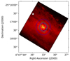 |
Fig. 1. Optical image from Hubble/WFC3 observations of the central ∼2′ of NGC 253. Overlays show the apertures used to extract the line fluxes from the different observatories. The apertures from Spitzer/IRS are shown in grey (SH; small rectangle) and black (LH; larger rectangle). The green square shows the footprint of the Herschel/PACS integral-field-unit. The blue circles are the apertures for the SOFIA/FIFI-LS observations of [O III]52 μ m (solid line), [O III]88 μ m (dashed line), [O I]146 μ m (dash-dotted line), and [C II]158 μ m (dotted line), as described in B22. See also Table 2. |
Owing to the large range of ionisation potentials and density regimes to excite these infrared emission lines, we are now able to draw a more complete picture of the embedded regions in the nucleus of NGC 253 and estimate the physical conditions there by modelling all lines simultaneously.
In addition to the line fluxes listed in Table 3 of B22 we also used observations of the CO rotational transitions CO(1−0) to CO(3−2) from Israel et al. (1995) and CO(4−3) to CO(8−7) from Pérez-Beaupuits et al. (2018) to compare a posteriori. Higher-J CO emission lines are also available in Pérez-Beaupuits et al. (2018). However, these lines are not available in the model grid (Sect. 2.2), and hence we could not use them as constraints or for a comparison a posteriori.
2.2. Model grid
The grid of models used in this study was Star-Forming Galaxy with an X-ray component (SFGX; Ramambason et al. 2022)1. SFGX is a grid of Cloudy (a 1D radiative transfer code, see Ferland et al. 2017) models assuming a cloud of spherical geometry. The modelled cloud is illuminated by a representative stellar cluster of a given age, t, and luminosity, L⋆. The spectrum of this star cluster is created with BPASS (Stanway & Eldridge 2018). In addition to the star cluster, an X-ray source with an inner disk temperature, TX2, and luminosity, LX, is modelled by a multi-colour black body (Mitsuda et al. 1984). In this study, we refer to this combination of star cluster and X-ray source, which are assumed to be co-spatial, as a “cluster”. A cluster in this context is described by a parameter set (L⋆, t, LX, TX). The X-ray source in these Cloudy models is particularly important in our study because of the presence of highly ionised emission lines such as [Ne V]14 μ m and [O IV]26 μ m. Ions like Ne4+ and O3+ with ionisation potentials > 54.9 eV (or λ = 22.6 nm) to create the ion are unlikely to be created by stars and likely imply the presence of an AGN or a different source of X-ray emission.
An ISM component in the grid is characterised by the metallicity, Z, the ionisation parameter, U, the hydrogen volume density at the illuminated edge of the cloud, n, and the depth. We emphasise that the metallicity refers to the O/H abundance. Other elements (such as N, Ne, C, Ne, and Si) scale with the O/H abundance – see Ramambason et al. (2022) for the respective relations. Since the luminosity is already included in the cluster properties, the ionisation parameter is defined by the distance, r, between the cloud and the cluster. SFGX was created to investigate physical conditions in low-metallicity galaxies. Since the optical depth, AV, as a function of depth varies with metallicity (i.e. two clouds with the same physical size but different metallicities have different AV), a more general definition of the cloud depth was defined by a “cut” parameter, ξ, as shown in Table 1.
Definition of the different values of the cut parameter, ξ, in the SFGX grid.
In the following, a parameter set (Z, U, n, ξ) is called a “component”. We note that in cases in which more than one component is modelled, the metallicity is the same for all components. The SFGX grid contains a total of 32 000 models, which are divided into 544 000 sub-models by introducing 17 cut values between ξ = 0 and ξ = 4. We refer to Ramambason et al. (2022) for more details about the grid of models and an application to the Herschel Dwarf Galaxy Survey (Madden et al. 2013).
2.3. Inference method
We used MULTIGRIS for the modelling approach (Lebouteiller & Ramambason 2022). MULTIGRIS uses a Bayesian approach, designed to calculate posterior probability density distributions of the parameters of a given grid of models by using priors (e.g. line fluxes and errors) as constraints. Upper and lower limits for line fluxes can be used as well.
MULTIGRIS allows a linear combination of components, or continuous distributions for the parameters. This is particularly important, as the ISM in galaxies is not homogeneous on (kilo-)parsec-scales, but instead heterogeneous and a mix of several components (e.g. Lacy et al. 1982; Burton et al. 1990; Snow & McCall 2006; Cormier et al. 2019). By considering several components or using, for instance, power laws (PLaws) for certain parameters, various geometries that are relevant to studies of complex objects like galaxies can be explored.
Hence, we investigated two different model architectures: a one cluster and two component architecture (1C2S), and an architecture in which U, n, ξ, and t are continuously distributed, following a PLaw. Both architectures have been used to model the ISM in galaxies; see for instance Péquignot (2008), Polles et al. (2019) approaches with a discrete sampling and Baldwin et al. (1995), Richardson et al. (2016), Ramambason et al. (in prep.) for continuous distribution of ISM parameters.
A power law approach, for instance for the depth and density, takes the porosity and clumpiness of the ISM into account by enabling a larger number of low-density (diffuse) clouds and only a few clouds of higher density and large depth, or vice versa. Each parameter that is described by a PLaw introduces three variables: the slope, α, of the PLaw, and the lower and upper boundaries between which the PLaw is valid.
The choice of a probabilistic approach is justified by the complexity of the problem, for example:
-
The combination of two or more components (i.e. stellar populations or gas phases) yields a large number of free parameters, making it difficult to gauge degenerate solutions.
-
Upper limits or asymmetric uncertainties of line fluxes are difficult to handle with deterministic approaches.
-
Known parameters (e.g. the metallicity) and their uncertainty cannot be used as priors in a deterministic approach.
Probabilistic tools such as MULTIGRIS are able to overcome all the mentioned issues of deterministic techniques. For more details about the methodology, sampling techniques, and applications of MULTIGRIS see Lebouteiller & Ramambason (2022).
We note that in B22 we listed the obtained line fluxes and statistical uncertainties in Table 3. The uncertainties did not include systematical or calibration errors. We included these uncertainties by defining line sets for each instrument. Each line set includes the emission lines observed by one instrument. We assumed that systematic and calibration uncertainties affect the observed emission lines of an instrument all in the same way. For each line set, we introduced a scaling parameter to account for these systematic and calibration uncertainties. This also allowed us to consider potential offsets due to the different spatial resolution and wavelength coverage, and hence the different size of the nucleus. In particular, we also divided the Spitzer/IRS emission lines into two observation sets since this instrument consists of two different modules with different aperture sizes, namely short-high (SH) and long-high (LH) modules. See the discussion in Sect. 2.3.2 of B22 for details.
3. Model of the ionised gas
In this first step we investigated model results using the emission lines arising from H II regions only, meaning all lines with an ionisation potential of ≥13.6 eV. We note that lines with a lower ionisation potential (for example [C II]158 μ m and [Si II]35 μ m) may also arise in H II regions (e.g. Abel et al. 2005; Chevance et al. 2016). However, we did not use these lines as constraints in the first step, because of their ambiguous origin. We let the model predict which fraction of [C II]158 μ m comes from the ionised gas only. This was done by comparing the cumulative line flux of [C II]158 μ m at the ionisation front and at the solution for the cut value, ξ. Lines with lower ionisation potentials are included in Sect. 4. Also, we note that the [Fe III]23 μ m emission line is not included – due to the strong dependence of Fe emission lines on the dust-to-gas ratio, these emission lines are handled separately (see Sect. 4.2).
Recently, Behrens et al. (2022) reported that the cosmic ray ionisation rate (CRIR) in selected clouds in the nuclear region of NGC 253 is about 104× larger than the average Galactic value ζ0 = 2 × 10⁻¹⁶ s−1 (Indriolo et al. 2007). The value of the CRIR used in SFGX, however, is only 3ζ0 (Ramambason et al. 2022). We show in Sect. 3.4 that cosmic rays only mildly affect the ionised gas, and hence the effect on the model results are negligible. The effect of the increased CRIR on the neutral atomic and molecular gas, however, is significant and is explored on a smaller sub-grid (see Sect. 4).
3.1. Systematic offsets within the dataset
In B22 we show the data reduction and cross-calibration of observations of NGC 253 with SOFIA, Spitzer, and Herschel. To account for potential offsets between the line sets (i.e. the emission lines as observed by one instrument) due to calibration or aperture effects, we performed MULTIGRIS runs in which the different line sets were successively added (i.e. the first run with IRS SH and LH modules, the second run adding the PACS lines etc.). MULTIGRIS determines the – small – systematic offsets between datasets so that observations match better with models. The LH module of Spitzer/IRS served as standard (i.e. offsetLH ≡ 1). As the aperture size of this instrument matches the angular size of the nucleus (6.68″) best, we believe that this observation contains low background emission and we therefore expect the LH line set to be of the best quality.
In this way, systematic offsets between line sets should be the dominant source of uncertainties. To simultaneously investigate the effect of different model architectures, we performed the same runs for a 1C2S and for a PLaw architecture. These architectures fulfil the request for more than one component as claimed in B22, but are still as simple as possible. Due to the limited number of constraints, a simple model with fewer parameters preferably avoids overfitting. Table 2 shows the obtained offsets between observation sets that will be further used in this work. Line fluxes shown in Table 3 of B22 were multiplied by these factors to account for the offsets introduced by calibration uncertainties and PSF effects between the instruments.
Mean systematic line flux offsets due to calibration or aperture effects between observation blocks determined from MULTIGRIS runs in linear scale.
The systematic offsets of all line sets are smaller than one. This could be due to different beam sizes, meaning that the Herschel and SOFIA observations include more background emission because of their lower spatial resolution. This would also explain why the PACS, SPIRE, and FIFI-LS offsets are all in good agreement. The SH observations of Spitzer/IRS are also < 1. Since this observation does not fully sample the nucleus due to a small aperture size, we performed a scaling correction of 1.55 based on the continua of SH and LH in B22. The lines may not arise from the exact same region as the thermal emission at ∼20 μm, which could lead to an over-correction of the line fluxes, and thus a systematic offset < 1 in the SH emission lines.
3.2. Impacts of the model configuration
To evaluate the performance, we used the marginal likelihood as well as “pnσ” values, both of which are computed by MULTIGRIS. The marginal likelihood measures the probability that the model grid including any prior reproduces the observations and will reach a maximum for the most likely set of parameters, under the assumption that the priors do not change. Too few parameters are not able to reproduce all the emission lines and will therefore have a low marginal likelihood, while too many parameters will cause overfitting, which is when the model contains more parameters than can be justified by the constraints. The pnσ values on the other hand describe how many draws of the posterior distribution agree within nσ of the constraints or observables. The higher the pnσ values, the better the model is able to reproduce the observations within their uncertainties.
Generally, both architectures show high pnσ values, with p3σ = 99.19% and p3σ = 96.44% for the 1C2S and PLaw architectures, respectively. Moreover, both are able to reproduce all emission lines (with the exception of [O IV]26 μ m) within the uncertainties (see Fig. 2). The log marginal likelihood is better for the 1C2S architecture (−31.8, compared to −37.3 for the PLaw architecture). However, this does not mean that the 1C2S architecture is a more realistic or “better” one – see for instance Lebouteiller & Richardson (in prep.) for a discussion on model architectures. To conclude, the model architecture does not seem to play a significant role in the modelling of the ionised gas.
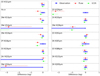 |
Fig. 2. Comparison of modelled/predicted and observed line fluxes. Emission lines from the ionised gas are used as constraints. The abscissa is normalised to the observed line flux (≡0) with errorbars (blue). Red and green show the resulting line fluxes from the PLaw and 1C2S architectures, respectively. For display reasons, the abscissa in column one are compressed so that the PLaw results for the [Ne V] lines are not entirely visible. Blue arrows denote the upper limits on line fluxes. |
3.3. Results for the ionised gas
We started by narrowing down the parameter space of our model grid. This is necessary, since a new model grid with a larger CRIR is required but the full set of Cloudy models would take a long time to run. To do so, we investigated the parameters that can already be determined from the solution for the ionised gas. For instance, emission lines from species with high ionisation potentials such as [O IV]26 μ m (55 eV) and [Ne V]14 μ m (97 eV) are almost exclusively created by X-rays (Abel & Satyapal 2008). Hence, the parameters of the X-ray source are already constrained when using these emission lines. Another parameter that can already be determined is the metallicity, Z, provided we assume that the metallicity does not vary significantly within the nuclear region. We further estimated the stellar luminosity, L⋆, using the ionised gas model, assuming that this parameter does not vary greatly once the neutral atomic gas lines are taken into account. We focus on the PLaw architecture in this section and compare the results with those from the 1C2S architecture at the end of this section. Figure 3 shows the probability density functions (PDF) of the parameters determined in this section. Mejía-Narváez et al. (2020) interpret the PDFs, for instance for the metallicity, as a physical distribution within the ISM; however, we think that the PDF in our case is dominated by the uncertainty rather than a physical metallicity distribution function. Table 3 shows the resulting median and standard deviations for all variables of the model. For the PLaw distributed parameters an average and standard deviation is given as well.
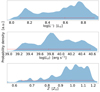 |
Fig. 3. Probability density distributions for the stellar luminosity, L⋆, X-ray luminosity, LX, and metallicity, Z, for the PLaw architecture (see Sect. 3.3). The median and confidence intervals of the posterior distribution are shown in red. |
Table 3 and Fig. 3 show that the inferred metallicity from the inference is around the solar value. This is in good agreement with the results of our analytic approach in B22, in which we calculated Z = 1.0 Z⊙ using the ([Ne II]13 μ m + [Ne III]16 μ m)/Hu α line flux ratio. The probability is a little outside the given uncertainties.
With  we obtained a somewhat lower stellar luminosity, L⋆, than previous studies, although with a large uncertainty and broad PDF, as can be seen in row 1 of Fig. 3. Watson et al. (1996) estimated a luminosity from young stars of 1.5 × 10⁹ L⊙. Radovich et al. (2001) calculated 1.5 × 10¹⁰ L⊙, although with a much poorer spatial resolution (∼2′) and a higher extinction correction of 11 mag, compared to our result of AV = 4.35 mag in B22.
The mean age of the nuclear stellar cluster that we obtain from our solution is  . This is slightly younger than previous estimates, such as by Kornei & McCrady (2009), Fernández-Ontiveros et al. (2009), who obtained 5.7 and 6.3 Myr, respectively, perhaps due to a different choice of initial mass functions (IMFs). We investigate the effects of different IMFs in Sect. 5.3.
One major question that is tackled with this study is the characterisation of the central BH, because the physical properties and the impact of the BH on the ISM are not completely understood. The total X-ray luminosity obtained from our models, which we assume originates in the central BH or AGN, is 5.9 × 1039 erg s−1, which is in good agreement with Chandra observations (4.7 × 1039 erg s−1; Lopez et al. 2023) and Fernández-Ontiveros et al. (2009). The X-ray luminosity shows large uncertainties, but the PDF shows only low probabilities for luminosities below 1039 erg s−1 and above 4 × 1040 erg s−1 (see in Fig. 3). To confirm that an X-ray component is important in this model, we made runs with no X-ray source. For both architectures, the pnσ values and marginal likelihood drop by several percent and the highly ionised emission lines are not well reproduced. The X-ray component is indeed necessary to model the observed emission lines, in particular to recover the [O IV] and [Ne V] emission. For comparison, Sgr A* has a similar luminosity of LX = 4 × 1039 erg s−1 (Kaneda et al. 1997), suggesting that the central BH of NGC 253 resembles a low-luminosity AGN rather than a typical extragalactic AGN that has luminosities in the range of LX = 1040 − 1043 erg s−1 (e.g. Fornasini et al. 2018).
The PLaw distributions of the density, n, the ionisation parameter, U, and the cut parameter, ξ, show that a model with low-density (i.e. diffuse), low-depth, and low ionisation parameter clouds is preferred. However, the range of these three parameters is small (see the lower and upper boundaries in Table 3), suggesting that most of the ionised gas emission arises from a mostly diffuse gas component. The average gas density in the PLaw model is 135 cm−3, which is in good agreement (although with large uncertainties) with our analytic results in B22, in which we used the [O III]52/88 μ m, [S III]19/33 μ m, and [N II]122/205 μ m line flux ratios and obtained 84 ≲ n ≲ 212 cm−3. As expected, the range of the cut values, ξ, is somewhat beyond the ionisation front, ξ = 1.0. A fraction of the emission from species with ionisation potentials near 13.6 eV (e.g. [N II]) possibly originates beyond the ionisation front, which is why ξ ≡ 1.0 or below is not an expected or reasonable solution.
In Table 3 we also show the resulting parameters for the 1C2S configurations. Both the PLaw and 1C2S architectures are in good agreement within the uncertainties, showing again that the choice of configurations seems to be only a second order effect when considering only the ionised gas emission lines.
3.4. Influence of cosmic rays
Using data from the ALCHEMI spectral survey (Martín et al. 2021), Behrens et al. (2022) show that the CRIR in the centre is three to four orders of magnitudes larger than the average Milky Way value, ζ0, while the value used in the SFGX grid is fixed at only 3ζ0. Such high values imply a considerable increase of heating to the ISM and will in particular affect emission lines from the neutral atomic and molecular gas (e.g. Sternberg & Dalgarno 1995; Goldsmith 2001; Bisbas et al. 2021). Here, we investigated if the higher CRIR also affects emission from the ionised gas. For this purpose, we created new Cloudy models using the best parameter set obtained from the model results in Sect. 3.3 and changed the CRIR from 6 × 10⁻¹⁶ s−1 to 10−13 s−1, as reported in Behrens et al. (2022). The Cloudy models were combined according to their weights or covering factors, Wi, as shown in Table 3. As expected, emission lines from the ionised gas are hardly affected by a change in the CRIR (see Fig. B.1). The difference in the cumulative line flux slightly beyond the ionisation front (i.e. ξ = 1.25) is lower than 10% for most of the lines. Only Hu α, [Ne II]13 μ m, and [S III]33 μ m have a larger but still small difference of ≲20%. Emission lines from the neutral atomic and molecular gas, however, are heavily affected by a change in the CRIR. Figures 4 and 5 show that the difference in these lines is of the order of one magnitude or even more.
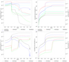 |
Fig. 4. Emissivity (left) and cumulative line flux (right) over the cut parameter, ξ, for emission lines from the ionised gas. The solid lines show models with a low CRIR (6 × 10⁻¹⁶ s−1) and the dashed lines are from models with a high CRIR (10−13 s−1). |
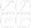 |
Fig. 5. Same as Fig. 4 but for emission lines from the molecular gas and the total infrared luminosity, LTIR. |
4. Modelling the ionised and neutral atomic gas
4.1. New model grid and sanity checks
To take the higher CRIR and their effect on the neutral atomic (and molecular) gas into account, we created a new sub-grid of SFGX with an increased CRIR of 10−13 s−1. To reduce the computing time for calculating the Cloudy models and for the MULTIGRIS runs, we decreased the parameter space as listed in Table 4. The resulting new grid contains a total of 10 880 models. We combined this new grid with the corresponding sub-grid from SFGX, so that we now had a sampling for the CRIR. We call this new grid SFNX (for “star-forming nucleus with an X-ray source”) in the following3.
Input parameters of Cloudy models in the new sub-grid of SFGX and the parameter space of the original SFGX grid.
In Sect. 3.4 we showed that an increased CRIR only has a minor impact on the line fluxes of ionised gas lines. To confirm that the effect is negligible, we proved that MULTIGRIS finds similar parameter sets in SFNX and in SFGX.
We carried out another run with a two component configuration, using only emission lines originating in the ionised gas, as done in Sect. 3.2. Table 3 shows the resulting mean values and confidence intervals for both runs, which are in good agreement. The only exception is LX, in which the results from the new grid are lower but still within the uncertainties. This is most likely due to a degeneracy effect between LX and ζ (see Sect. 5.1 for a more detailed discussion) and the higher values chosen for L⋆ = 109 L⊙ in order to be consistent with the SFGX grid. Since the new grid is able to reproduce the results from SFGX, but also takes the much higher CRIR into account, we were now able to investigate solutions for the neutral atomic gas.
4.2. Results for the ionised and neutral atomic gas
In the next step we added emission lines from the neutral atomic gas, with the systematic offsets as determined in Sect. 3.1 remaining the same.
As mentioned earlier, we had not yet included the [Fe III]23 μ m emission line due to the dependence on the dust-to-gas ratio. Adding emission lines from the neutral atomic gas such as [Fe II]18 μ m and [Fe II]26 μ m as constraints, we now enabled a small systematic offset for the three Fe lines. We assumed that the line fluxes scale linearly with the iron abundance (within only a small offset) and accounted for small variations in the dust-to-gas ratio. We obtain an offset of ∼0.3 for both configurations, suggesting that the model would under-predict the Fe lines without the scaling.
Since H2 rotational transitions arise to a significant extent from the warm neutral atomic gas (e.g. Roussel et al. 2007; Togi & Smith 2016) we also include these lines in these new runs. Although we include emission lines from molecular hydrogen, we do not claim that our model is a proper solution for the molecular gas in the centre of NGC 253.
Most of the parameters obtained for the ionised gas model (Sect. 3.3 and Table 3) are consistent with the model of the ionised and neutral atomic gas, as shown in Table 5. This shows that the approach of starting with only ionised gas lines and determining systematic offsets between instruments (Sect. 3.1) is valid. Generally, the preferred model in the PLaw architecture has a high abundance of low-density, low ionisation parameter, and low-depth (i.e. diffuse gas) clouds. All three parameters (n, U, and ξ) have a negative slope for the PLaw, meaning that higher-density clouds with larger depths and higher ionisation parameters are less abundant. In the 1C2S architecture, this is reflected by a smaller covering factor, W2, for the second component. However, some parameters show differences compared to the results from the ionised gas. Obviously, the cut parameter, ξ, is larger than in the model for the ionised gas. To reproduce emission lines from the neutral atomic gas, the model has to reach values beyond the ionisation front (ξ = 1) and even the H/H2 photo-dissociation front (ξ = 2). Since we do not include CO or other emission lines from the molecular core, larger depths (ξ ≥ 3) are neither needed nor found. The obtained average, ξ ≈ 2.3 (cf. Table 1), translates into an AV of 4.5, which is in good agreement with our results in B22 (see also Fig. A.1). Furthermore, the density – in particular the upper limit, nupper, of the PLaw architecture and the density of the second component, n2, of the 1C2S architecture – is significantly higher than in the ionised gas model. This is expected, since the model needs to account for higher critical densities of many of the emission lines from the warm neutral gas, such as [O I]63 μ m or [Si II]35 μ m.
Resulting parameters from an inference using emission lines from the ionised and neutral atomic gas as constraints, for the two different architectures discussed in this study.
The additional parameter introduced for the CRIR, ζ, is ∼2 × 10⁻¹⁵ s−1. This is significantly lower than predicted by Behrens et al. (2022; ∼10−13 s−1), which is expected for two reasons. First, the region observed is much larger in our case (40″ compared to 1.6″ in Behrens et al. 2022), so the locally increased CRIR from Behrens et al. (2022) is smeared out within our observing beam. Second, although many lines are sensitive to the CRIR, as shown in Sect. 3.4, higher fluxes for these lines can be modelled for instance by a higher density, a stronger radiation field, and/or a higher X-ray luminosity (see Sect. 5.1). It is possible that there is some degeneracy between these parameters, which may also be reflected by the large uncertainties.
Some of the emission lines are not reproduced by any of the architectures (e.g. [N II]122 μ m or [Fe II]26 μ m), resulting in lower pnσ values, now with a p3σ of 85% compared to ≥95%. See Fig. 6 for a comparison of observed and modelled line fluxes for both architectures. The pnσ values are, however, still high enough to obtain a reliable inference of further (secondary) parameters from this model (Sect. 5.4).
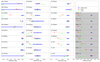 |
Fig. 6. Same as Fig. 2. Emission lines from the ionised and neutral atomic gas are used as constraints (white background) with CO emission lines predicted by MULTIGRIS (grey background). |
5. Discussion
5.1. Cosmic ray ionisation rate and X-ray luminosity
Table 3 shows that the X-ray luminosity drops significantly from ∼5 × 1039 erg s−1 to ∼1037 erg s−1 once the CRIR is increased. This somewhat contradicts our finding that X-rays are needed to reproduce the highest ionised emission lines in our sample. Hence, we performed another MULTIGRIS run, forcing a higher X-ray luminosity of LX = 5 × 1039 erg s−1. The resulting parameter sets for both architectures (PLaw and 1C2S) are similar, with the exception of the CRIR, which drops by ∼25% in the higher X-ray runs, consistent with findings from Lebouteiller et al. (2017). Cosmic rays affect mostly the neutral atomic and molecular gas, while the ionised gas remains unchanged. X-rays, however, affect the ionised gas – and high ionisation states in particular – but also heat the neutral atomic gas, which creates a degeneracy between the luminosity of the X-ray source and the CRIR. Such difficulties between the discrimination of X-rays and cosmic rays have already been shown, for instance by Meijerink et al. (2006). Observations of the CO+ molecule could help to break this degeneracy, as done in M82 (Spaans & Meijerink 2007). In conclusion, this implies that both the CRIR and X-ray luminosity obtained in this study (Tables 3 and 5) should be considered rather as upper limits.
5.2. Predictions for the molecular gas
From the PDFs of the model parameters, MULTIGRIS is able to predict the luminosity of other emission lines. We predicted line fluxes for several CO emission lines (J = 1 → 0 to J = 8 → 7) that arise from the molecular gas. We compared the predicted line fluxes with those observed by Herschel/PACS and Herschel/SPIRE (see Pérez-Beaupuits et al. 2018) but did not use them as constraints. Figure 6 compares the observed and predicted CO line fluxes and the corresponding uncertainties in column 4 (grey background). With the exception of CO(1 − 0) in the 1C2S architecture, all CO emission lines are under-predicted by up to two orders of magnitude. The model clearly fails to account for the molecular gas.
We investigated potential causes of the under-prediction of the CO emission. However, for a more detailed model of the molecular gas we refer to a forthcoming paper. Due to the increased CRIR, the ISM is much warmer and the H/H2 and C/CO photo-dissociation front are shifted to larger depths with increasing ζ. Since the Cloudy models, however, stop at a fixed AV = 10 mag, models with a higher CRIR contain less H2, and therefore also less CO. This, in turn, results in significantly lower CO line fluxes simply due to the low abundance of CO in the whole Cloudy model. To overcome the low CO abundance, we investigated which AV is needed to predict the observed CO line fluxes by running new Cloudy models with parameters from Table 5 but with an arbitrary high AV of 30 mag. In fact, such a model would be able to reproduce the CO line fluxes as observed by Herschel/SPIRE and JCMT, but the increase in depth obviously affects other lines in the model as well. In particular, emission lines like the [C I] and [O I] lines originate partly in the molecular gas and become brighter with larger depth (see also Fig. 4, which shows that the cumulative fluxes of these lines are growing even at larger ξ values). Furthermore, we calculated the total molecular hydrogen mass, M(H2), from these high AV models (see Sect. 5.4), which is two orders of magnitude larger than typical hydrogen masses in the nuclei of galaxies. To conclude, simply increasing the depth of the models cannot overcome the under-predicted CO emission, which other emission lines would be affected by and from which an absurdly high molecular gas mass would be obtained. Furthermore, it would be in contradiction with our results for an AV of 4.35 from the SED fit in B22.
Shocks could also play a role in the excitation of CO emission (e.g. Lesaffre et al. 2013; Pon et al. 2016; Kamenetzky et al. 2018). Furthermore, Hao et al. (2009) showed that shocks can possibly excite [O IV]26 μ m emission, which is significantly under-predicted in our models as well. Another mechanism not taken into account is the time-dependence of the chemistry. Cloudy assumes a static chemistry; however, simulations have shown that a time-dependent chemistry (in particular in nuclei of active galaxies) can result in CO line fluxes that are several orders of magnitude brighter (Meijerink et al. 2013).
5.3. Effects of the initial mass function
To determine the emitted spectrum of an interstellar cloud, Cloudy requires an input spectrum, in our case the spectrum of a starburst cluster. The distribution of the overall mass among the stars within the cluster (the IMF) can have a significant effect on the output spectrum of the cluster, and hence also on the physical conditions and spectrum of the illuminated cloud. However, the exact shape of the IMF, and whether it universal, is still uncertain and debated (e.g. Hopkins 2018, and references therein). We analysed the impact of a different IMF by creating a new input spectrum. To eliminate potential uncertainties by using different codes (and therefore different assumptions such as evolutionary tracks, etc.), we used BPASS to predict the stellar emission.
While the other parameters remained the same (Eldridge et al. 2017; Ramambason et al. 2022), we changed the IMF from a Kroupa-like IMF (Kroupa et al. 1993) to a Salpeter IMF (Salpeter 1955). Thereafter, we ran two Cloudy simulations with the parameters from Table 5, one using the spectrum from a Kroupa IMF and one using the spectrum from a Salpeter IMF.
Figure 7 shows the resulting line fluxes from these Cloudy simulations. The line fluxes from the two models are generally in good agreement, in particular emission lines originating in the neutral atomic (e.g. [O I] and [C I]) and molecular gas (CO and H2), where they agree within 1%. Emission lines, which to some fraction come from the ionised gas, are slightly more affected. The [Fe II], [C II]158 μ m, and [Si II]35 μ m lines differ by ∼5%. The largest deviations occur for emission lines that arise purely from the ionised gas, with the Kroupa IMF yielding fainter line fluxes than the Salpeter IMF in almost all cases. For instance, the two [Si III] lines are brighter by ∼10% and the two [Ne III] lines by ∼20%. However, the ratio of two emission lines from the triplet of a species (e.g. [N II], [S III], and [O III]) are constant for one IMF. This indicates that the reason for the differences is primarily different abundances of the respective ions. Indeed, the abundance of higher ionic states (which is one output of Cloudy) are 5 − 10% higher for the Kroupa IMF at depths lower than the ionisation front.
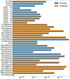 |
Fig. 7. Comparison of predicted line fluxes from Cloudy runs, using a Kroupa (blue) and Salpeter (orange) IMF input spectrum, respectively. For representation reasons, the [Ne V] emission lines are not shown but are both of the order of 10−28 W m−2, i.e. within the upper limits of our observations. |
We conclude that the particular shape of the chosen IMF can have a significant impact on the resulting line fluxes, in particular those from emission lines originating in the ionised gas. However, by selecting a state-of-the-art IMF and model BPASS, we assume that these effects are minor and that our results are valid.
5.4. Secondary parameters obtained from the model
In addition to predicting line fluxes of other emission lines, MULTIGRIS also allows us to predict secondary parameters in post-processing runs. These secondary parameters must be stored in a post-processing grid that is associated with the main grid, in our case SFGX and SFNX, respectively. The values listed throughout this section are results from the PLaw architecture. However, similar to the results of the primary parameters in Table 5, the post-processing parameters are comparable and agree within uncertainties. Assuming a spherical geometry, the masses of dust and the different hydrogen phases were calculated from the Cloudy output. Using our final model (see Table 5) we are then able to estimate the mass of ionised and neutral atomic hydrogen in the centre of NGC 253. In principle, we can also obtain a mass for the molecular hydrogen. However, due to the limited validity of our model regarding the molecular gas, the results for this phase have to be taken with caution, as noted by the large uncertainties associated with these parameters. The resulting masses are shown in Table 6. Both the mass for the ionised hydrogen and that for the neutral atomic hydrogen are in good agreement with estimates from KAO observations (Carral et al. 1994), which obtained 1 × 10⁶ M⊙ and 5 × 10⁶ M⊙ from the Tielens & Hollenbach (1985) PDR models for the ionised and neutral atomic hydrogen, respectively.
Resulting post-processing parameters for the nucleus of NGC 253.
We can also estimate the fraction of [C II]158 μ m associated with the ionised, neutral atomic, and molecular gas. Recently, [C II] has been increasingly considered as a probe for the CO dark gas or even the total molecular gas mass (e.g. Madden et al. 2020, and references within). It is necessary, however, to correct for emission coming from H II regions that do not contain any H2. In the case of NGC 253 with solar metallicity, the fraction of [C II]158 μ m from the ionised gas phase is ∼26% (see Table 6). This is somewhat lower than the findings in Cormier et al. (2019) (using their Eq. (2) yields 45% of [C II]158 μ m from the ionised gas), which could be due to the different CRIR assumed in our study or the fact that solar metallicities are not covered in Cormier et al. (2019).
5.5. Star formation rates
In Sect. 3.3 we showed that the potential AGN in the centre of NGC 253 has little effect on its environment, as probed by the observed lines. What really drives the heating in the nucleus seems to be the star formation activity, usually quantified by the star formation rate (SFR). Within the last few decades, a number of tracers for the SFR have been proposed, either from theoretical considerations or empirical calibrations (see Kennicutt & Evans 2012, for a review). Each of these tracers has its (dis-)advantages, in particular regarding where the respective probe arises, and if it is affected by extinction. In this section we compare three different SFR tracers, namely the Hα, [C II]158 μ m, and LTIR luminosities. Throughout, we assume a distance of 3.5 Mpc (Rekola et al. 2005) to convert fluxes to luminosities.
One of the most important tracers of the SFR is the luminosity of the Hα line, since it is easily observable with optical telescopes and is directly emitted by young stars. From our latest model presented in Sect. 4, MULTIGRIS is able to infer the intrinsic (extinction-free) luminosity of this emission line (Table 6). Using the empirical calibration from Calzetti et al. (2007), which is also tested on smaller, ∼100 pc scales (Pessa et al. 2021; Belfiore et al. 2023), we obtain  . One disadvantage of the Hα emission line is that that it that it typically suffers from extinction in extragalactic sources, which is why we corrected the line flux from Table 6 assuming a mixed extinction model and the optical depth of 4.5 mag, as determined in Sect. 4.2.
Another frequently employed probe for the SFR is the total infrared luminosity, LTIR. It assumes that in thermal equilibrium most of the stellar radiation is reprocessed by dust and radiated within the infrared spectral range (i.e. between 3 μm and 1000 μm). We already determined the LTIR in B22 in two different ways, confirmed by our MULTIGRIS approach. The calibration shown in Kennicutt (1998) yields  , which is in good agreement with the SFR determined from Hα.
Stacey et al. (1991) proposed the [C II]158 μ m emission line as a probe for the SFR. Since we directly measured this quantity and did not calculate or predict it, we believe that this is the most reliable measurement of the SFR in this study – not taking any calibration uncertainties into account. Using the more recent calibration from Herrera-Camus et al. (2018), we obtain SFR = 1.7 ± 0.5 M⊙ yr−1.
All the SFRs we obtain from the different probes are in good agreement with each other. They are also comparable with the results from ISO observations in Radovich et al. (2001), who obtained SFR = 2.1 M⊙ yr−1 for the nucleus; however, with a larger beam of the ISO telescope compared to our observations. The larger observing beam could result in contamination of infrared emission from the disk, and therefore in a slightly higher SFR. Yet, the result from Radovich et al. (2001) is within the uncertainties of our solution.
5.6. Comments on, and caveats for, the model grids
Although the model grids SFGX and SFNX that we use cover a wide range of ISM conditions, we note that some mechanisms are not taken into account, which might affect the model results and in particular lead to the under-prediction of the CO emission lines. These aspects are discussed shortly and will be further investigated in future studies.
According to Sánchez (2020) and Sánchez et al. (2021), one potential major contribution to the radiation field could be post-asymptotic giant branch (AGB) stars. These objects typically have a hard but weak ionising effect on the ISM, which could cascade down into the CO-emitting regions. AGB stars are included in the BPASS models; however, the post-AGB phase is not well understood and needs improvements (Eldridge et al. 2017). While the works of Sánchez (2020), Sánchez et al. (2021) show that ionisation occurs on local scales, the limited spatial resolution of our observations in this work leads to the fact that the ionising sources are not resolved.
Another mechanism not considered in the model grids is shocks, for instance from supernovae or galactic outflows. Such outflows have been observed in CO, Hα, and X-ray emission (Bolatto et al. 2013). They are well known to contribute to ISM heating, and therefore boost emission lines.
Lastly, the relative abundances of elements vary not only within galaxies but even when comparing H II regions within one galaxy (García-Rojas & Esteban 2007). The model grids take into account that the abundance, for example of N and C, varies with the O/H ratio. However, it might also be the case that the relative abundance of N and C changes as well. A deviation in the relative abundances of elements would directly lead to a change in the relative line fluxes of different species.
6. Summary
In this study we used a combined set of 30 emission lines from SOFIA, Herschel, and Spitzer observations of the nuclear region of the starburst galaxy NGC 253 to investigate the physical conditions of the ISM on a 100 pc scale. Using MULTIGRIS, a Bayesian code to probabilistically investigate a set of Cloudy models, we constrained the parameters of the ionised and neutral atomic gas. After eliminating systematic offsets between the different telescopes, instruments, and modules, we first determined the parameters of the ionised gas. The model we created is able to reproduce all observed emission lines, with the exception of [O IV]26 μ m. We find that the metallicity and density that we calculated from analytic prescriptions in B22 are in good agreement with our probabilistic results. Furthermore, we infer that the hypothetical AGN in the nucleus of NGC 253 has a minor impact on the heating of the ISM, with luminosities ≲6 × 1039 erg s−1 or ≲1.5 × 10⁶ L⊙. After modelling the ionised gas, we added emission lines originating in the neutral atomic gas, with an increased CRIR, as shown by Behrens et al. (2022). We show that the higher CRIR has little to no effect on the results for the ionised gas. Again, the extended model is able to reproduce most (24 of 30) of the emission lines, and the obtained optical depth is in good agreement with our results from B22. However, the model fails to reproduce most of the CO emission – we refer to a future study to further investigate the molecular gas properties. From our model we were able to calculate gas and dust masses, and determined the fraction of [C II]158 μ m emission from the different phases (Table 6). Since the nuclear starburst seems to have a major heating impact on the ISM, we calculated the star formation rates from different tracers, which are all in good agreement (0.6 − 1.7 M⊙ yr−1).
SFGX is available within the MULTIGRIS framework at https://gitlab.com/multigris/mgris
The outer disk temperature is assumed to be a constant TX, out = 103 K.
Available at https://doi.org/10.5281/zenodo.8362031
Acknowledgments
We thank the referee, S. Sánchez, for comments which improved the clarity of the paper. The authors acknowledge support by the state of Baden-Württemberg through bwHPC. L.R. gratefully acknowledges funding from the DFG through an Emmy Noether Research Group (grant number CH2137/1-1).
References
- Abel, N. P., & Satyapal, S. 2008, ApJ, 678, 686 [NASA ADS] [CrossRef] [Google Scholar]
- Abel, N. P., Ferland, G. J., Shaw, G., & van Hoof, P. A. M. 2005, ApJS, 161, 65 [NASA ADS] [CrossRef] [Google Scholar]
- Baldwin, J., Ferland, G., Korista, K., & Verner, D. 1995, ApJ, 455, L119 [NASA ADS] [Google Scholar]
- Beck, A., Lebouteiller, V., Madden, S. C., et al. 2022, A&A, 665, A85 [NASA ADS] [CrossRef] [EDP Sciences] [Google Scholar]
- Behrens, E., Mangum, J. G., Holdship, J., et al. 2022, ApJ, 939, 119 [NASA ADS] [CrossRef] [Google Scholar]
- Belfiore, F., Leroy, A. K., Sun, J., et al. 2023, A&A, 670, A67 [NASA ADS] [CrossRef] [EDP Sciences] [Google Scholar]
- Bisbas, T. G., Tan, J. C., & Tanaka, K. E. I. 2021, MNRAS, 502, 2701 [CrossRef] [Google Scholar]
- Bolatto, A. D., Warren, S. R., Leroy, A. K., et al. 2013, Nature, 499, 450 [Google Scholar]
- Burton, M. G., Hollenbach, D. J., & Tielens, A. G. G. M. 1990, ApJ, 365, 620 [NASA ADS] [CrossRef] [Google Scholar]
- Calzetti, D., Kennicutt, R. C., Engelbracht, C. W., et al. 2007, ApJ, 666, 870 [Google Scholar]
- Carral, P., Hollenbach, D. J., Lord, S. D., et al. 1994, ApJ, 423, 223 [NASA ADS] [CrossRef] [Google Scholar]
- Chevance, M., Madden, S. C., Lebouteiller, V., et al. 2016, A&A, 590, A36 [NASA ADS] [CrossRef] [EDP Sciences] [Google Scholar]
- Cormier, D., Abel, N. P., Hony, S., et al. 2019, A&A, 626, A23 [NASA ADS] [CrossRef] [EDP Sciences] [Google Scholar]
- Eldridge, J. J., Stanway, E. R., Xiao, L., et al. 2017, PASA, 34, e058 [Google Scholar]
- Engelbracht, C. W., Rieke, M. J., Rieke, G. H., Kelly, D. M., & Achtermann, J. M. 1998, ApJ, 505, 639 [NASA ADS] [CrossRef] [Google Scholar]
- Ferland, G. J., Chatzikos, M., Guzmán, F., et al. 2017, Rev. Mex. Astron. Astrofis., 53, 385 [NASA ADS] [Google Scholar]
- Fernández-Ontiveros, J. A., Prieto, M. A., & Acosta-Pulido, J. A. 2009, MNRAS, 392, L16 [CrossRef] [Google Scholar]
- Fornasini, F. M., Civano, F., Fabbiano, G., et al. 2018, ApJ, 865, 43 [NASA ADS] [CrossRef] [Google Scholar]
- García-Rojas, J., & Esteban, C. 2007, ApJ, 670, 457 [CrossRef] [Google Scholar]
- Goldsmith, P. F. 2001, ApJ, 557, 736 [Google Scholar]
- Günthardt, G. I., Agüero, M. P., Camperi, J. A., et al. 2015, AJ, 150, 139 [CrossRef] [Google Scholar]
- Hao, L., Wu, Y., Charmandaris, V., et al. 2009, ApJ, 704, 1159 [NASA ADS] [CrossRef] [Google Scholar]
- Herrera-Camus, R., Sturm, E., Graciá-Carpio, J., et al. 2018, ApJ, 861, 95 [Google Scholar]
- Hopkins, A. M. 2018, PASA, 35, e039 [NASA ADS] [CrossRef] [Google Scholar]
- Indriolo, N., Geballe, T. R., Oka, T., & McCall, B. J. 2007, ApJ, 671, 1736 [NASA ADS] [CrossRef] [Google Scholar]
- Iodice, E., Arnaboldi, M., Rejkuba, M., et al. 2014, A&A, 567, A86 [NASA ADS] [CrossRef] [EDP Sciences] [Google Scholar]
- Israel, F. P., White, G. J., & Baas, F. 1995, A&A, 302, 343 [NASA ADS] [Google Scholar]
- Kamenetzky, J., Privon, G. C., & Narayanan, D. 2018, ApJ, 859, 9 [Google Scholar]
- Kaneda, H., Makishima, K., Yamauchi, S., et al. 1997, ApJ, 491, 638 [NASA ADS] [CrossRef] [Google Scholar]
- Kennicutt, R. C., Jr. 1998, ApJ, 498, 541 [Google Scholar]
- Kennicutt, R. C., & Evans, N. J. 2012, ARA&A, 50, 531 [NASA ADS] [CrossRef] [Google Scholar]
- Kornei, K. A., & McCrady, N. 2009, ApJ, 697, 1180 [NASA ADS] [CrossRef] [Google Scholar]
- Kroupa, P., Tout, C. A., & Gilmore, G. 1993, MNRAS, 262, 545 [NASA ADS] [CrossRef] [Google Scholar]
- Lacy, J. H., Beck, S. C., & Geballe, T. R. 1982, ApJ, 255, 510 [NASA ADS] [CrossRef] [Google Scholar]
- Lebouteiller, V., & Ramambason, L. 2022, A&A, 667, A34 [NASA ADS] [CrossRef] [EDP Sciences] [Google Scholar]
- Lebouteiller, V., Péquignot, D., Cormier, D., et al. 2017, A&A, 602, A45 [NASA ADS] [CrossRef] [EDP Sciences] [Google Scholar]
- Lesaffre, P., Pineau des Forêts, G., Godard, B., et al. 2013, A&A, 550, A106 [NASA ADS] [CrossRef] [EDP Sciences] [Google Scholar]
- Lopez, S., Lopez, L. A., Nguyen, D. D., et al. 2023, ApJ, 942, 108 [NASA ADS] [CrossRef] [Google Scholar]
- Madden, S. C., Rémy-Ruyer, A., Galametz, M., et al. 2013, PASP, 125, 600 [NASA ADS] [CrossRef] [Google Scholar]
- Madden, S. C., Cormier, D., Hony, S., et al. 2020, A&A, 643, A141 [NASA ADS] [CrossRef] [EDP Sciences] [Google Scholar]
- Martín, S., Mangum, J. G., Harada, N., et al. 2021, A&A, 656, A46 [NASA ADS] [CrossRef] [EDP Sciences] [Google Scholar]
- Meijerink, R., Spaans, M., & Israel, F. P. 2006, ApJ, 650, L103 [Google Scholar]
- Meijerink, R., Spaans, M., Kamp, I., et al. 2013, J. Phys. Chem. A, 117, 9593 [NASA ADS] [CrossRef] [Google Scholar]
- Mejía-Narváez, A., Sánchez, S. F., Lacerda, E. A. D., et al. 2020, MNRAS, 499, 4838 [CrossRef] [Google Scholar]
- Melo, V. P., Pérez García, A. M., Acosta-Pulido, J. A., Muñoz-Tuñón, C., & Rodríguez Espinosa, J. M. 2002, ApJ, 574, 709 [NASA ADS] [CrossRef] [Google Scholar]
- Mitsuda, K., Inoue, H., Koyama, K., et al. 1984, PASJ, 36, 741 [NASA ADS] [Google Scholar]
- Péquignot, D. 2008, A&A, 478, 371 [NASA ADS] [CrossRef] [EDP Sciences] [Google Scholar]
- Pérez-Beaupuits, J. P., Güsten, R., Harris, A., et al. 2018, ApJ, 860, 23 [Google Scholar]
- Pessa, I., Schinnerer, E., Belfiore, F., et al. 2021, A&A, 650, A134 [NASA ADS] [CrossRef] [EDP Sciences] [Google Scholar]
- Polles, F. L., Madden, S. C., Lebouteiller, V., et al. 2019, A&A, 622, A119 [NASA ADS] [CrossRef] [EDP Sciences] [Google Scholar]
- Pon, A., Kaufman, M. J., Johnstone, D., et al. 2016, ApJ, 827, 107 [NASA ADS] [CrossRef] [Google Scholar]
- Puche, D., & Carignan, C. 1991, ApJ, 378, 487 [NASA ADS] [CrossRef] [Google Scholar]
- Radovich, M., Kahanpää, J., & Lemke, D. 2001, A&A, 377, 73 [NASA ADS] [CrossRef] [EDP Sciences] [Google Scholar]
- Ramambason, L., Lebouteiller, V., Bik, A., et al. 2022, A&A, 667, A35 [NASA ADS] [CrossRef] [EDP Sciences] [Google Scholar]
- Rekola, R., Richer, M. G., McCall, M. L., et al. 2005, MNRAS, 361, 330 [NASA ADS] [CrossRef] [Google Scholar]
- Richardson, C. T., Allen, J. T., Baldwin, J. A., et al. 2016, MNRAS, 458, 988 [NASA ADS] [CrossRef] [Google Scholar]
- Roussel, H., Helou, G., Hollenbach, D. J., et al. 2007, ApJ, 669, 959 [NASA ADS] [CrossRef] [Google Scholar]
- Salpeter, E. E. 1955, ApJ, 121, 161 [Google Scholar]
- Sánchez, S. F. 2020, ARA&A, 58, 99 [Google Scholar]
- Sánchez, S. F., Walcher, C. J., Lopez-Cobá, C., et al. 2021, Rev. Mex. Astron. Astrofis., 57, 3 [Google Scholar]
- Snow, T. P., & McCall, B. J. 2006, ARA&A, 44, 367 [NASA ADS] [CrossRef] [Google Scholar]
- Spaans, M., & Meijerink, R. 2007, ApJ, 664, L23 [NASA ADS] [CrossRef] [Google Scholar]
- Stacey, G. J., Geis, N., Genzel, R., et al. 1991, ApJ, 373, 423 [NASA ADS] [CrossRef] [Google Scholar]
- Stanway, E. R., & Eldridge, J. J. 2018, MNRAS, 479, 75 [NASA ADS] [CrossRef] [Google Scholar]
- Sternberg, A., & Dalgarno, A. 1995, ApJS, 99, 565 [NASA ADS] [CrossRef] [Google Scholar]
- Tielens, A. G. G. M., & Hollenbach, D. 1985, ApJ, 291, 747 [NASA ADS] [CrossRef] [Google Scholar]
- Togi, A., & Smith, J. D. T. 2016, ApJ, 830, 18 [NASA ADS] [CrossRef] [Google Scholar]
- Vogler, A., & Pietsch, W. 1999, A&A, 342, 101 [NASA ADS] [Google Scholar]
- Wall, W. F., Jaffe, D. T., Israel, F. P., & Bash, F. N. 1991, ApJ, 380, 384 [NASA ADS] [CrossRef] [Google Scholar]
- Watson, A. M., Gallagher, J. S., III, Holtzman, J. A., et al. 1996, AJ, 112, 534 [NASA ADS] [CrossRef] [Google Scholar]
- Weiß, A., Kovács, A., Güsten, R., et al. 2008, A&A, 490, 77 [NASA ADS] [CrossRef] [EDP Sciences] [Google Scholar]
Appendix A: Relation between AV and ξ
The definition of the cut parameter, ξ (Table 1), is linked to the density of the ionisation states of hydrogen. Therefore, the optical (and physical) depth of the ξ values changes with the ambient conditions, such as the density, n, ionisation parameter, U, or metallicity, Z. Specifically, there is no equation describing the relation between ξ and AV. Figure A.2 illustrates the relation between these two parameters, with changing ambient conditions from Cloudy models. The “Std” model (blue line) shows the resulting AV vs ξ relation, with a parameter set of log n = 2 cm−3, log U = −3, and Z = 1 Z⊙, which is close to the final parameter set (Sect. 4.2). Red, green, and cyan lines show the relation with changing density (log n = 4 cm−3), the ionisation parameter (log U = −1), and the metallicity, Z = 0.5 Z⊙, respectively.
Figure A.1 shows the kernel-density-estimate plots from the MULTIGRIS run of a 1C2S configuration, as described in Sect. 4. This illustrates which values for ξ1 and ξ2 are a likely solution, and to which AV these correspond. The spread in the AV for similar ξ, in particular in the top panel, corresponds to the different physical conditions (e.g. different metallicities or densities).
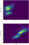 |
Fig. A.1. Kernel density estimate (KDE) plots showing the relation between AV and ξ from the MULTIGRIS runs, as described in Sect. 4, for a 1C2S configuration. |
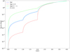 |
Fig. A.2. Relation between AV and ξ from Cloudy models with different ISM parameters. The “Std” model results from a parameter set with log n = 2 cm−1, log U = −3, and Z = 1 Z⊙. The legend denotes which parameters were changed. |
Appendix B: Effects of cosmic rays on emission lines from the ionised gas
For completeness reasons, we show the emissivity and cumulative line fluxes of lines from the ionised gas for two different CRIR, ζ (see Sect. 3.4). Since cosmic rays do not dominate the heating in H II regions, the effect of an increased CRIR – in particular before the ionisation front (ξ = 1) – is negligible.
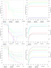 |
Fig. B.1. Emissivity (left) and cumulative line flux (right) over the cut parameter, ξ, for emission lines from the ionised gas. Solid lines show models with a low CRIR (6 × 10⁻¹⁶ s−1). Dashed lines are from models with a high CRIR (10−13 s−1). |
All Tables
Mean systematic line flux offsets due to calibration or aperture effects between observation blocks determined from MULTIGRIS runs in linear scale.
Input parameters of Cloudy models in the new sub-grid of SFGX and the parameter space of the original SFGX grid.
Resulting parameters from an inference using emission lines from the ionised and neutral atomic gas as constraints, for the two different architectures discussed in this study.
All Figures
|
Fig. 1. Optical image from Hubble/WFC3 observations of the central ∼2′ of NGC 253. Overlays show the apertures used to extract the line fluxes from the different observatories. The apertures from Spitzer/IRS are shown in grey (SH; small rectangle) and black (LH; larger rectangle). The green square shows the footprint of the Herschel/PACS integral-field-unit. The blue circles are the apertures for the SOFIA/FIFI-LS observations of [O III]52 μ m (solid line), [O III]88 μ m (dashed line), [O I]146 μ m (dash-dotted line), and [C II]158 μ m (dotted line), as described in B22. See also Table 2. |
| In the text | |
|
Fig. 2. Comparison of modelled/predicted and observed line fluxes. Emission lines from the ionised gas are used as constraints. The abscissa is normalised to the observed line flux (≡0) with errorbars (blue). Red and green show the resulting line fluxes from the PLaw and 1C2S architectures, respectively. For display reasons, the abscissa in column one are compressed so that the PLaw results for the [Ne V] lines are not entirely visible. Blue arrows denote the upper limits on line fluxes. |
| In the text | |
|
Fig. 3. Probability density distributions for the stellar luminosity, L⋆, X-ray luminosity, LX, and metallicity, Z, for the PLaw architecture (see Sect. 3.3). The median and confidence intervals of the posterior distribution are shown in red. |
| In the text | |
|
Fig. 4. Emissivity (left) and cumulative line flux (right) over the cut parameter, ξ, for emission lines from the ionised gas. The solid lines show models with a low CRIR (6 × 10⁻¹⁶ s−1) and the dashed lines are from models with a high CRIR (10−13 s−1). |
| In the text | |
|
Fig. 5. Same as Fig. 4 but for emission lines from the molecular gas and the total infrared luminosity, LTIR. |
| In the text | |
|
Fig. 6. Same as Fig. 2. Emission lines from the ionised and neutral atomic gas are used as constraints (white background) with CO emission lines predicted by MULTIGRIS (grey background). |
| In the text | |
|
Fig. 7. Comparison of predicted line fluxes from Cloudy runs, using a Kroupa (blue) and Salpeter (orange) IMF input spectrum, respectively. For representation reasons, the [Ne V] emission lines are not shown but are both of the order of 10−28 W m−2, i.e. within the upper limits of our observations. |
| In the text | |
|
Fig. A.1. Kernel density estimate (KDE) plots showing the relation between AV and ξ from the MULTIGRIS runs, as described in Sect. 4, for a 1C2S configuration. |
| In the text | |
|
Fig. A.2. Relation between AV and ξ from Cloudy models with different ISM parameters. The “Std” model results from a parameter set with log n = 2 cm−1, log U = −3, and Z = 1 Z⊙. The legend denotes which parameters were changed. |
| In the text | |
|
Fig. B.1. Emissivity (left) and cumulative line flux (right) over the cut parameter, ξ, for emission lines from the ionised gas. Solid lines show models with a low CRIR (6 × 10⁻¹⁶ s−1). Dashed lines are from models with a high CRIR (10−13 s−1). |
| In the text | |
Current usage metrics show cumulative count of Article Views (full-text article views including HTML views, PDF and ePub downloads, according to the available data) and Abstracts Views on Vision4Press platform.
Data correspond to usage on the plateform after 2015. The current usage metrics is available 48-96 hours after online publication and is updated daily on week days.
Initial download of the metrics may take a while.