| Issue |
A&A
Volume 681, January 2024
|
|
|---|---|---|
| Article Number | A14 | |
| Number of page(s) | 23 | |
| Section | Interstellar and circumstellar matter | |
| DOI | https://doi.org/10.1051/0004-6361/202347280 | |
| Published online | 22 December 2023 | |
Modeling the molecular gas content and CO-to-H2 conversion factors in low-metallicity star-forming dwarf galaxies
1
Institut fur Theoretische Astrophysik, Zentrum für Astronomie, Universität Heidelberg,
Albert-Ueberle-Str. 2,
69120
Heidelberg,
Germany
e-mail: This email address is being protected from spambots. You need JavaScript enabled to view it.
2
Université Paris Cité, Université Paris-Saclay, CEA, CNRS, AIM,
91191,
Gif-sur-Yvette,
France
3
Physics Department, Elon University,
100 Campus Drive CB 2625,
Elon,
NC
27244,
USA
4
Department of Physics & Astronomy, University College London,
Gower Street,
London
WC1E 6BT,
UK
5
Sterrenkundig Observatorium, Ghent University,
Krijgslaan 281–S9,
9000
Ghent,
Belgium
6
Cosmic Origins Of Life (COOL) Research DAO, coolresearch.io
7
University of Cincinnati, Clermont College,
4200 Clermont College Drive,
Batavia,
OH
45103,
USA
8
AURA for ESA, Space Telescope Science Institute,
3700 San Martin Drive,
Baltimore,
MD
21218,
USA
9
Laboratoire d’Astrophysique de Bordeaux, Univ. Bordeaux, CNRS,
B18N, Allée Geoffroy Saint-Hilaire,
33615
Pessac,
France
Received:
25
June
2023
Accepted:
5
October
2023
Abstract
Context. Low-metallicity dwarf galaxies often show no or little CO emission, despite the intense star formation observed in local samples. Both simulations and resolved observations indicate that molecular gas in low-metallicity galaxies may reside in small dense clumps, surrounded by a substantial amount of more diffuse gas that is not traced by CO. Constraining the relative importance of CO-bright versus CO-dark H2 star-forming reservoirs is crucial to understanding how star formation proceeds at low metallicity.
Aims. We test classically used single component radiative transfer models and compare their results to those obtained on the assumption of an increasingly complex structure of the interstellar gas, mimicking an inhomogeneous distribution of clouds with various physical properties.
Methods. Using the Bayesian code MULTIGRIS, we computed representative models of the interstellar medium as combinations of several gas components, each with a specific set of physical parameters. We introduced physically motivated models assuming power-law distributions for the density, ionization parameter, and the depth of molecular clouds.
Results. This new modeling framework allows for the simultaneous reproduction of the spectral constraints from the ionized gas, neutral atomic gas, and molecular gas in 18 galaxies from the Dwarf Galaxy Survey. We confirm the presence of a predominantly CO-dark molecular reservoir in low-metallicity galaxies. The predicted total H2 mass is best traced by [C II]158 μm and, to a lesser extent, by [C I] 609 μm, rather than by CO(1–0). We examine the CO-to-H2 conversion factor (αCO) versus metallicity relation and find that its dispersion increases significantly when different geometries of the gas are considered. We define a “clumpiness” parameter that is anti-correlated with [C II]/CO and explains the dispersion of the αCO versus metallicity relation. We find that low-metallicity galaxies with high clumpiness parameters may have αCO values as low as the Galactic value, even at low metallicity.
Conclusions. We identify the clumpiness of molecular gas as a key parameter for understanding variations of geometry-sensitive quantities, such as αCO. This new modeling framework enables the derivation of constraints on the internal cloud distribution of unresolved galaxies, based solely on their integrated spectra.
Key words: galaxies: starburst / galaxies: dwarf / ISM: structure / radiative transfer / infrared: ISM / methods: numerical
© The Authors 2023
 Open Access article, published by EDP Sciences, under the terms of the Creative Commons Attribution License (https://creativecommons.org/licenses/by/4.0), which permits unrestricted use, distribution, and reproduction in any medium, provided the original work is properly cited.
This article is published in open access under the Subscribe to Open model. This email address is being protected from spambots. You need JavaScript enabled to view it. to support open access publication.
1 Introduction
Quantifying the total amount of molecular gas hosted within a galaxy is an important step to understand how stars form in different environments. The presence of cold molecular gas is thought to be a necessary element with respect to fueling the formation of new stars through the fragmentation of dense molecular clouds (e.g., Chevance et al. 2023). Its direct detection is complicated by the fact that H2 has no electric dipole moment. While rovibrational H2 emission can be detected in the infrared, the latter only traces a warm (E/k ≳ 510 K, Roueff et al. 2019) H2 component, rather than the total H2 mass. As an alternative, CO emission has been extensively used to probe the colder H2 component in large samples of local galaxies with instruments such as IRAM, APEX (e.g., HERACLES; Leroy et al. 2009, xCOLD gas survey; Saintonge et al. 2017, Montoya Arroyave et al. 2023), and ALMA (e.g. ALMA-PHANGS, Leroy et al. 2021), in systems at intermediate redshift (z < 1, e.g., Freundlich et al. 2019), and up to redshifts of ~6 (e.g., Ginolfi et al. 2017; Boogaard et al. 2023).
Nevertheless, converting the CO emission into estimates of the total molecular gas masses is not straightforward. A first complication comes from the fact that the CO-to-H2 conversion factor (hereafter, αCO in pc−2(K km s−1)−1) is sensitive to internal variations of the physical properties of the interstellar medium (ISM), rendering the interpretation of an averaged galactic value difficult. At galactic scales, the αCO conversion factor can be derived as a statistical average for the populations of CO-emitting clouds, assuming, in particular, that they are virialized and not overlapping (e.g., Dickman et al. 1986; Bolatto et al. 2013, hereafter B13). Nevertheless, important cloud-to-cloud variations are expected within the ISM of galaxies (e.g., Sun et al. 2020, 2022), making the αCO values particularly sensitive to the spatial variations within galaxies.
In particular, radial gradients of αCO have been observed in local spiral galaxies (e.g., Teng et al. 2022; den Brok et al. 2023) with lower conversion factors derived in galactic centers (e.g., Sandstrom et al. 2013). Environmental effects may also impact star formation mechanisms, leading to dependencies of the αCO values on global galactic parameters (e.g., Accurso et al. 2017). In particular, both the metallicity and dust content of galaxies strongly impact the αCO values (e.g. Glover & Mac Low 2011; Schruba et al. 2012; Bolatto et al. 2013; Genzel et al. 2015; Amorín et al. 2016; Accurso et al. 2017; Tacconi et al. 2018; Madden et al. 2020). Recently, Hirashita (2023) suggested that the αCO conversion factor may be sensitive not only to the dust-to-gas mass ratio but also to the size distribution of dust grains, which impacts the formation and destruction pathways of both H2 and CO molecules. In low-metallicity and dust-poor galaxies, the radiation field may penetrate deep into the molecular cloud envelopes and photodis-sociate CO molecules, while H2 may remain self-shielded. As a result, large amounts of “CO-dark” (e.g., Wolfire et al. 2010) H2 gas, invisible in CO, have been reported in low-metallicity galaxies (e.g., Poglitsch et al. 1995; Madden et al. 1997, 2020; Schruba et al. 2012, 2017; Amorín et al. 2016; Cormier et al. 2014).
Several methods have been explored to recover the fraction of molecular gas hidden in this CO-dark gas component. Direct detections of high-rotational level H2 in the mid-IR can be used to infer the warm and total H2 masses, based on assumptions related to the distribution of H2 rotational temperatures (Togi & Smith 2016). This method is especially promising in the context of JWST, which enables new detections of mid-IR H2 lines with an unprecedented sensitivity (e.g., Hernandez et al. 2023). At low metallicities, however, direct H2 detection remains challenging and alternative methods relying on indirect CO-dark gas tracers are needed. While Galactic studies can rely on numerous indirect tracers, including, for example, γ-ray emission (e.g., Grenier et al. 2005; Ackermann et al. 2012; Remy et al. 2018; Hayashi et al. 2019) or molecular absorption lines (e.g., Liszt & Lucas 1996; Lucas & Liszt 1996; Allen et al. 2015; Nguyen et al. 2018), studies of external galaxies must rely on the direct emission of luminous tracers associated with H2 reservoirs. In particular, the dust continuum has been classically used to estimate the total H2 mass in massive galaxies (e.g., Magnelli et al. 2012; Sandstrom et al. 2013; Genzel et al. 2015; Tacconi et al. 2018; Zavala et al. 2022), as well as in the small Local Group spiral galaxy M33 (Z ~ Z⊙; e.g., Braine et al. 2010; Gratier et al. 2017) and in the SMC (Tokuda et al. 2021).
The [C II]158 µm emission line also provides a widely used proxy of the molecular gas content (e.g., Zanella et al. 2018; Béthermin et al. 2020; Dessauges-Zavadsky et al. 2020), including in dwarf galaxies (e.g., Jameson et al. 2018; Madden et al. 2020) and a potentially promising proxy for high-redshift studies (e.g., Vizgan et al. 2022). More recently, the [C I] emission line has also been identified as a potential tracer of the molecular gas (e.g., Jiao et al. 2019; Crocker et al. 2019; Madden et al. 2020; Dunne et al. 2021, 2022), although its detection remains relatively more challenging.
A proper calibration of the αCO conversion factor, accounting for the CO-dark component, is crucial for solving long-standing debates regarding star formation mechanisms in low-metallicity environments. Among other aspects, the lack of H2 and CO emission in star-forming low-metallicity galaxies (e.g., Tacconi & Young 1987; Taylor et al. 1998; Cormier et al. 2014, 2017; Leroy et al. 2007) could indicate unusually high star formation efficiencies at low metallicity (e.g., Turner et al. 2015). Alternative scenarios include the existence of mechanisms preventing the formation of H2 molecules, particularly due to the smaller amount of dust grains on which H2 form or their disruption in the aftermath of star formation. It also could possibly serve as evidence for the existence of star-formation pathways directly in the neutral atomic gas (e.g., Glover & Clark 2012a,b), with important implications for star formation at high-redshift.
While primordial galaxies remain beyond the reach of current CO-observing facilities, local low-metallicity dwarf galaxies with CO measurements are ideal for investigating those questions. In Madden et al. (2020, hereafter M20), we analyzed a sample of nearby star forming low-metallicity galaxies from the Dwarf Galaxy Survey (DGS; Madden et al. 2013). Using the wealth of available infrared spectral tracers to constrain radiative transfer models, we inferred the total H2 mass in each galaxy of this sample. Our results suggest that most of their molecular mass may reside in CO-dark layers. Accounting for this CO-dark component, M20 reported that these dwarf galaxies fall back on the Kennicutt–Schmidt (KS) relation that links star formation rates (SFR) and stellar masses, from which they were significantly offset when accounting only for the CO-visible H2 mass.
While radiative transfer models, such as those used in M20 enable a deeper understanding of the underlying physics of the ISM than empirical studies, they rely on strong modeling assumptions. In particular, the Cloudy models used in M20 assumed a simple geometry, with the emission arising from the neutral ISM (atomic and molecular phase) matched by a single component (single metallicity and single ionizing source). This simplification of the actual complexity of the multiphase ISM was necessary to keep a reasonably low number of free parameters and to use the CO emission as a direct constraint on the visual extinction of molecular clouds (AV). Nevertheless, it prevented the performance of a fully consistent optimization of the free parameters, since AV was manually adjusted a posteriori to match the observed CO emission. Under those assumptions, M20 found a strong anti-correlation of AV with the [C II]/CO emission line ratio and an anti-correlation between αCO and AV. Because visual extinction is (by design) correlated with the gasphase metallicity in single component models, the latter results also imply an anti-correlation of the αCO with metallicity. M20 reported a negative slope of the αCO versus the metallicity relation, with a narrow dispersion (< 0.32 dex) of the DGS galaxies around it.
In the current study, we explore a more realistic set-up by relaxing the geometrical constraints imposed in M20. We use a new modeling framework, enabling the combination of multiple ISM components. This “topological” representation follows that introduced in Péquignot (2008) and extensively applied to galaxies, including those drawn from the DGS (Cormier et al. 2012, 2019; Polles et al. 2019; Lebouteiller et al. 2017). Those models require the simultaneous determination of numerous free parameters, which is difficult to robustly achieve with frequentist methods such as an X2 minimization. This difficulty was leveraged by the development of MULTIGRIS1 (Lebouteiller & Ramambason 2022a), which provides a new framework for model combination based on Bayesian statistics. While this new tool has successfully allowed for the modeling of the ionized and neutral ISM of the DGS galaxies with unprecedentedly detailed models (up to four components; Lebouteiller & Ramambason 2022b; Ramambason et al. 2022), this representation can still be improved. In particular, the use of statistical distributions to parameterize the combination of numerous components has been introduced in several recent studies to describe the hydrogen density and ionization parameter (Richardson et al. 2014, 2016, 2019), as well as the visual extinction (Bisbas et al. 2021) of clouds distributed within the ISM. These distribution functions provide a different representation, closer to what is predicted by simulations of a gravoturbulent star-forming ISM (e.g., Offner et al. 2014; Burkhart 2018; Burkhart & Mocz 2019; Appel et al. 2023) and observed in the nearby universe (e.g., Brunt 2015; Lombardi et al. 2015)
The work presented here uses the new ISM modeling framework from MULTIGRIS to revisit the M20 results, assuming a more complex geometry. The data used in this analysis, including updated CO measurements, is presented in Sect. 2. In Sect. 3, we describe the different architectures of models (single and multi-component). We compare their results to previous models from M20 and motivate the choice of an optimal architecture in Sect. 4. We then focus on the results obtained using the power law models in Sect. 5. The physical interpretations, caveats, and possible improvements of our study are discussed in Sect. 6. Our main findings are summarized in Sect. 7.
2 Data
2.1 Sample
Our sample is drawn from the DGS survey (Madden et al. 2013) which gathers observations of 50 nearby (0.5–191 Mpc) star-forming dwarf galaxies. This sample spans a large range of physical conditions and in particular a wide range of sub-solar2 metallicities from 12 + log(O/H) = 7.14 (~1/35 Z⊙) up to 8.43 (~ 1/2 Z⊙). This sample has been observed both in the far-infrared and submillimeter domains with the Herschel Space Telescope, as well as in the mid-infrared (MIR) domain with the Spitzer observatory. The wealth of emission lines arising from the different phases of the ISM makes it an ideal sample to constrain in detail the ISM structure. We restricted our sample to 18 compact galaxies for which either a detection or an upper limit in CO was available for the whole galaxy. We excluded galaxies for which only partial regions were observed.
In Table 1, we list the CO(1–0) measurements and upper limits taken from the literature, with their associated uncertainties. This table is based on that used in M20 but includes updated measurements and their reported uncertainties. Most measurements are expressed in K km s−1 and are reported with the instrumental beam θ, expressed in arcseconds. We also report the CO conversion to integrated flux in W m−2 based on Solomon et al. (1997), assuming that the angular size of the source was negligible compared to the telescope beam: ΩS ≪ Ωb. Hence, we approximate the solid angle of the source convolved with the telescope beam ΩS*b ≈ Ωb ≈ θ2, with θ the full width at half maximum of the telescope beam in arcsecs.
This assumption is equivalent to fixing arbitrarily the size of the source, which is unknown. It introduces uncertainties linked to the potential presence of CO emission outside the beam, which could lead to an underestimation of the molecular gas masses. Most importantly, Cormier et al. (2014) have stressed that this uncertainty may hamper the comparison between different CO line transitions, corresponding to different beam sizes, since their ratio is quite sensitive to the choice of beam used for the reduction. Thus, in the current study, we focus only on the CO(1–0) line, for which the largest number of detections are available. We note that transitions of higher energy level (e.g., CO(20–1) and CO(3–2)) as well as emission from 13CO have also been detected in a few galaxies, which we do not include in the current study. Nevertheless, for the two lowest metallicity galaxies in our sample for which no CO(1–0) detection is reported, we used conversions based on other transitions. For SBS 0335-052, we used the CO(3–2) detection reported in Hunt et al. (2014) to estimate CO(1–0) luminosity, assuming an area of 1″ subtended by the source. For I Zw 18, we use the CO(2–1) detection reported in Zhou et al. (2021) at 3.5σ significance, which they used to estimate a CO(1–0) luminosity, assuming an optically thick and thermalized emission.
Finally, we include the two recent CO(1–0) detections with the ALMA 12-m array for Haro 11 and NGC 1705, reported in Gao et al. (2022) and Hunt et al. (2023), respectively. Considering the new detections (rather than the previous upper limits on CO) lowers the predicted αCO values by a factor of ~72 for Haro 11 and a factor of ~6 for NGC 1705. Nevertheless, the predictions obtained for all the main quantities discussed throughout the paper (emission lines, masses, and conversion factors) remain compatible with the previous values within error-bars3. While the exact values of physical parameters are slightly modified (e.g., up to a factor ~3 for the predicted H2 masses), it does not change any of the trends discussed throughout the paper.
Hunt et al. (2023) also reported another detection obtained for NGC 1705 with the ACA 7-m array, which is a factor of two lower. To account for this uncertainty on the integrated flux, we considered a large σ value of half the ALMA 12-m detection to have a detection uncertainty of 50% of the total flux. Two new measurements for NGC 625 and NGC 5253 are also provided in Hunt et al. (2023). We included the updated measurement for NGC 5253, assuming an uncertainty of 10%, as the new value differs significantly from the value from Taylor et al. (1998) that was previously used in M20 (lower by a factor 2.5). Using the new detection yields an H2 mass that is lower by a factor 2.2, and a αCO value higher by a factor 1.14. As for Haro 11 and NGC 1705, those variations are smaller than the errorbars associated with our predictions. The ALMA 12-m integrated luminosity reported in Hunt et al. (2023) for NGC 625 corresponds to a luminosity of 6.59 × 10⁻²⁰ W m−2, which is slightly lower but compatible within errorbars with the measurement from Cormier et al. (2014) used in the current study.
Integrated CO(1–0) measurements in the DGS galaxies.
IR tracers used as constraints and corresponding ionization potentials for ionic lines.
2.2 Tracers of multi-phase ISM
In Table 2, we list the spectral tracers used as constraints. The tracers used to constrain the ionized gas and the photodissociated regions (PDR) are similar to those used in Ramambason et al. (2022). In addition to those tracers, the current analysis requires the use of tracers emitted in the molecular gas. As we will discuss in Sect. 5.2.1, the choice of tracers associated with molecular gas is not straightforward, especially in low-metallicity environments. In particular, part of the H2 may form in the PDR due to the self-shielding of H2 molecules. Hence, PDR tracers are particularly useful to estimate the total amount of molecular gas mass. When available, we include the following tracers that partly or totally emit in the PDRs: [O I], [Fe II], [Si II], and [C II].
As opposed to Ramambason et al. (2022), we do not include the H2 rovibrational lines as constraints, which consist mostly of upper limits, and use CO(1–0) instead. This exclusion is motivated by the coarse radial depth sampling in our models (see Sect. 3.1.2), which does not capture the sharp transition in the H2 cumulative emission. As shown in Fig. A.1, the emission of H2 may sharply increase before the H/H2 transition (defined in terms of fractional abundances). Because this transition is not well captured, this creates an abrupt jump in our predictions, with models stopping at the ionization front predicting no H2 emission, while all models stopping after the ionization front predict substantial H2 emission. As a result, our model predictions can only match the H2 upper limits with models that are completely deprived of molecular gas and PDR. Nevertheless, we checked a posteriori how the predicted H2 luminosities compare with the H2 detections and upper limits, as shown in Fig. A.2. We find that H2 S(0) and H2 S(1) upper limits are systematically over-predicted by our models, while this issue is somehow mitigated for the H2 detections. We find that our predictions agree within 0.5 dex with all the H2 detections, despite slight overpredictions of H2 S(0) and H2 S(1). The coarse radial sampling does not affect CO predicted emission, which has a smoother radial profile and probes a colder molecular gas reservoir, at larger AV (see Fig. A.1). This motivates the choice of our sample, described in Sect. 2.1, for which CO(1–0) measurements or upper limits are available.
3 Modeling framework
3.1 SFGX grid
3.1.1 Overview
The individual models or “components” used in this study are drawn from the “Star-Forming Galaxies with X-ray sources” (SFGX) grid of models presented in Ramambason et al. (2022), tailored to study star-forming low-metallicity dwarf galaxies. This grid consists of spherical models computed with the photoionization and photodissociation code Cloudy v17.02 (Ferland et al. 2017) and spans a large metallicity range going from ~1/100Z⊙ to 2Z⊙. Eight parameters were varied, associated with the physical properties of the radiation sources (the stellar luminosity, age of the stellar burst, X-ray luminosity, and temperature of the X-ray source assumed to be a multicolor blackbody) and the gas (metallicity, density at the illuminated edge, n, and ionization parameter, U, at the illuminated edge). The ionization parameter at the illuminated edge is defined as follows:
 (1)
(1)
where Q(H0) is the number of ionizing photons emitted per second, and n0 is the density at the illuminated edge, located at the inner radius Rin.
The SFGX grid has since been updated from the previous version used in Ramambason et al. (2022), with the addition of the dust-to-gas mass ratio (Zdust) as a free parameter (further described in Sect. 3.1.4). This additional free parameter increases the size of the grid by a factor of 3, leading to a total number of 96 000 Cloudy models covering nine free parameters. Each model is then cut into 17 sub-models stopping at different depths in the cloud, controlled by the “cut” parameter, following a procedure described in Sect. 3.1.2. These submodels allow us to account for “naked” H II regions that are either density-bounded or radiation-bounded and not associated with any neutral gas, as well as for embedded regions, associated with a layer of neutral gas, with varying thickness controlled by its cut. In the following section, we provide an overview of the characteristics of the SFGX grid which matters the most in the present study, including this cut parameter. We refer to Ramambason et al. (2022) for a complete description of the models. We now briefly recall the characteristics of three key parameters in the current study: radial density profile of Cloudy models, depth sampling, and dust-to-gas mass ratio.
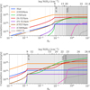 |
Fig. 1 Cumulative emission lines profiles of some chosen tracers as a function of the visual extinction AV, for two models drawn from the SFGX grid. Both models are computed with a density at the illuminated edge of 100 cm−2, an ionization parameter at the illuminated edge U = 10−2, an instantaneous stellar burst of 3 Myr computed with BPASS stellar atmospheres (Eldridge et al. 2017), and no X-ray source. The top row shows a solar metallicity model, while the bottom row shows amodel with Z = 1/10 Z⊙ and Zdust = 1/155 Zdust,⊙, following the prescription from Sect. 3.1.4. The shaded areas mark the location of the PDR (light gray) and molecular zone (dark gray). The vertical dashed lines show the cuts considered for each model. We note that the C/CO transition is not visible in the first panel since it occurs after AV = 10. |
3.1.2 Radial sampling
All models are computed until they reach either an AV of 10 or their electron temperature drops to 10 K4. Each initial Cloudy model is used to create 17 sub-models stopping at different AV controlled by the “cut” parameter, shown in Figs. 1 and 2. The transitions are defined in using the relative abundances of hydrogen (x(H+), x(H), and x(H2)) and carbon (x(C) and x(CO)), where x is the fractional abundance, normalized by the total abundance of a given element. The original model is successively cut at the inner radius (cut=0), ionization front (cut=1; x(H+)=x(H)), H2 dissociation front (cut=2; x(H)=x(H2)), CO dissociation front (cut=3; x(C)=x(CO)), and outer radius (cut=4).
To sample the different phases (H II region, PDR, CO-dark H2 gas, and CO-bright H2 gas) defined by those cuts, three additional cuts are added between each integer i (cut=i+0.25, i+0.5, i+0.75), equally spaced in AV between cut=i and cut=i+1. We note that stopping the model at a given cut and truncating it a posteriori is not strictly equivalent but results in minor variations of the emission, in the case of spherical models in which gas is only illuminated from one single side. Figure 1 illustrates the sampling in depth for two models drawn for the SFGX grid and the cumulative emission of some key tracers used to constrain the depth of a given component (see Sect. 2.2).
3.1.3 Radial density profile
The initial hydrogen density, corresponding to the illuminated edge of the models, is varied from 1 cm−3 to 104 cm−3. To consistently describe the density profile throughout the H II region, the PDR, and the molecular gas, we adopt the same density law as in Cormier et al. (2019), in which the hydrogen density is nearly constant in the H II region and scales with the total hydrogen column density above 1021 cm−2, as follows:
 (2)
(2)
where n0 is the hydrogen density at the illuminated edge and N(H) is the hydrogen column density. This law describes a smoothly varying density, matching both the density profile expected in the PDR of confined, dynamically-expanding H II regions (Hosokawa & Inutsuka 2005, 2006), and in the interior of turbulent molecular clouds (Wolfire et al. 2010).
As shown in Fig. 2, this prescription results in a smooth increase of density throughout the PDR and molecular zone, as opposed to the sharp variations expected, for instance, in the case of constant pressure models (see discussion in Cormier et al. 2019). Although this prescription is fixed in our grid, the resulting geometry of the models depends on other parameters such as the metallicity, ionization parameter, or the hardness of the radiation field. In particular, the depth of the PDR is strongly affected by the metallicity. In models with low metal and dust content, photons can propagate deeper and produce a thicker PDR than in solar-like metallicity models, as shown in Fig. 2.
3.1.4 Dust-to-gas mass ratio
Dust is included in our Cloudy models following the prescription described in Ramambason et al. (2022). The radial variation of the dust abundance follows that of the hydrogen density, while the total dust mass is set by assuming a metallicity-dependent dust-to-gas mass (Zdust). We consider three dust-to-gas mass ratio values per metallicity bin, by sampling the Zdust vs. metallicity relation derived in Galliano et al. (2021). This calibration relies on the spectral fitting of the infrared continuum for a large sample of DustPedia (Davies et al. 2017) and DGS galaxies, which includes our sample. They provide analytical fits corresponding to median, upper and lower values of the envelope encompassing 95% of the galaxies used in their analysis. These prescriptions allow us to explore the potential effects of Zdust variations on our predicted quantities, while restricting the exploration to plausible values of Zdust (within the 95% envelope) for each metallicity bin. We note that this prescription is more refined than the free power-law fit previously derived in Rémy-Ruyer et al. (2013), although compatible. Specifically, Rémy-Ruyer et al. (2013) predict that Zdust scales with ~Z−2, when assuming a metallicity-dependent αCO. For a metallicity of 1/10 Z⊙, the dust-to-gas mass ratio is scaled by a factor ~1/100, while the prescription from Galliano et al. (2021) results in a scaling of ~ 1/155. Although our grid is not designed to investigate in detail the dust composition and its radial distribution (which are both fixed), it remains flexible enough to self-consistently reproduce the observed integrated dust masses of galaxies (see Sect. 4.2).
3.2 MULTIGRIS runs
We applied the Bayesian code MULTIGRIS (Lebouteiller & Ramambason 2022a) to the sample of galaxies described in Sect. 2.1. This code enables flexible combinations of “components” drawn from a large grid of pre-computed models; here, this refers to the SFGX grid described in Sect. 3.1.1. The code architecture, based on the python package PyMC3 (Salvatier et al. 2016a,b), samples the parameter space assuming a given likelihood and sampling method, chosen by the user to infer posterior probability distribution functions (PDF) of any parameter. In the current study, we adopted a multi-Gaussian likelihood and a Markov chain Monte Carlo (MCMC) sampler, which is ideally suited to deal with multi-modal distributions (sequential Monte Carlo sampler, Minson et al. 2013; Ching & Chen 2007). Those choices are motivated and detailed in Lebouteiller & Ramambason (2022b) and Ramambason et al. (2022).
Specifically, our aim is to infer the posterior PDFs of the gas masses associated with different phases of the ISM, namely: M(H+), the total gas mass associated with the ionized reservoir as traced by H+. M(H0), the total gas mass associated with the neutral hydrogen reservoir as traced by H0; M(H2), the total gas mass associated with the molecular gas reservoir as traced by H2; and Mdust, the total mass of dust.
Those masses are extracted from each individual Cloudy models considered as “components”, following the procedure described in Sect. 3.2.1. We also derive those quantities for more complex architectures that consist of either linear combinations of a discrete number of components (see Sect. 3.2.2) or are based on statistical distributions for some key parameters (see Sect. 3.2.3).
3.2.1 Single component models
For each Cloudy model, the total gas mass, MH,i, associated with a given hydrogen state (H+, H0, or H2) is computed as follows:
 (3)
(3)
where mH,i is the mass of the hydrogen ion or molecule (H+, H0, or H2) used as tracer, nH,i is the density of this tracer, xH,i is the relative abundance of the tracer with respect to total hydrogen, nH is the density of total hydrogen, r is the radius varying between the inner (Rin) and outer (Rout) radius, and 4πr2dr is the volume of shell of gas between the radius r and r + dr.
We derived an estimate of the total dust mass based on the dust-to-gas mass ratio, Zdust, defined in Sect. 3.1.4. The total dust mass is defined by:
 (4)
(4)
where Zdust is the dust-to-gas mass ratio, Y⊙ is the Galactic mass fraction of Helium, and M(H+), M(H0), and M(H2) are defined by Eq. (3). In the rest of the paper, we adopt Y0 = 0.270 (Asplund et al. 2009), leading to a corrective factor for the helium mass of ~1.36.
The gas mass definition introduced in Eq. (3) relies on the use of radial abundance profile of hydrogen atoms, under different states. This definition is flexible and can easily be adapted to trace the gas reservoir of ionized, neutral, or molecular gas associated with other elements (e.g., carbon). We define the gas reservoir in different phases as the integrated hydrogen mass, weighted by the fractional abundance of a given tracer as follows:
 (5)
(5)
where  is the density of the element X in a given ionization state (or molecular form), j, and
  is the fractional abundance of this tracer with respect to the total density of the element X. By design, we note that
  . We applied this formula to derive the mass of H2 in the different carbon phases:
  , M(H2)C, and M(H2)CO.
3.2.2 A few independent components
We define a multi-component architecture as a linear combination of components, using a mixing-weight. Those models represent a galaxy as a mix of N different gas components, associated with independent sets of gas parameters (U, n, cut, and the mixing-weight; 4N free parameters), sharing similar chemical properties (described by two parameters; the gas-phase metallicity and dust-to-gas mass ratio) and illuminated by the same radiation field (i.e., a single representative cluster of stars, described by four free parameters: the stellar age, the total cluster luminosity, the luminosity, and temperature of a potential X-ray source). The number of free parameters for such models, including the mixing-weights, is thus 4N + 6, where N is the number of gas components. We refer to Ramambason et al. (2022) for further details, in which a larger sample of DGS galaxies was modeled with architectures combining up to three components.
We define multi-component models by computing linear combinations for the extensive quantities of linear components, in particular, the integrated luminosities and gas masses. To first order, we assume that the gas masses scale linearly with the observed luminosity. In other words, our multi-component models can be considered as luminosity-weighted combination of gas components. We computed the total masses (i.e., M(H2), M(H I), M(H II), and Mdust), and the H2 masses in different carbon phases (i.e., M(H2)C+, M(H2)C, and M(H2)CO) as linear combinations of the masses of each component, such that:
 (6)
(6)
where wi is the mixing-weight and Mi the predicted mass associated with a specific ISM phase, for the ith component. The same formula is applied to derive the combined total luminosity of a given line.
As shown in Ramambason et al. (2022), multi-component models with one to three components enable a simultaneous reproduction of most of the emission lines arising from the H II regions and PDRs in the DGS. Nevertheless, the tailored model developed for IZw 18 in Lebouteiller & Ramambason (2022b), which includes additional tracers of the molecular gas (e.g., CO), has required the addition of a fourth component, corresponding to a component that is deep enough to reach the denser molecular phase in which CO is emitted, associated with a relatively small mixing-weight. Thus, in the current study, we follow a similar approach and consider models with up to four independent components.
We use the same selection criterion as in Ramambason et al. (2022) to select the optimal number of components and keep only the best configuration, according to the marginal likelihood metric. The values for the relative marginal likelihoods and the number of components chosen in the best configuration are reported in Table A.1. We note that models that have the largest number of components do not necessarily perform better in terms of marginal likelihood. This comes from the fact that numerous free parameters (e.g., 4 × 4 + 6 = 22 free parameters for a four-component model) penalize models when not enough constraints are available. To solve this issue, in the following section, we present another architecture allowing for a combination of large numbers of components, while keeping a relatively low number of free parameters.
3.2.3 Statistical distributions of components
While it is possible (in theory) to apply the linear combination described in Sect. 3.2.2 to a large (>4) number of components, the resulting models are associated with lower marginal likelihoods, reflecting the fact that the solution is diluted in an increasingly large parameter space. Instead, we generalize the combination of models by combining components drawn from statistical distributions defined analytically.
A first simple approach is to describe the key parameters of our models using power-law distributions. This approach was inspired by the locally optimally emitting cloud model (LOC; Baldwin et al. 1995), previously used to reproduce emission lines from the narrow line region in quasars and star-forming galaxies (Ferguson et al. 1997; Richardson et al. 2014, 2016). The latter models consider power laws to describe the distributions of density and radiation field of H II regions, allowing for the representation of the integrated emission of a population of clouds with various densities, distributed at various distances from an ionizing source. In the current study, we used the ionization parameter, U, as a proxy for the strength of the radiation field and consider an additional power law describing the depth of each component (via the cut parameter, described in Sect. 3.1.2). This is in essence similar to the approach based on AV-PDF used, for instance, in Bisbas et al. (2019, 2023), albeit here with different choices for the prior distributions, which we further discuss in Sect. 6.2.2.
As detailed in Table 3, we use power-law distributions to describe the three main gas parameters of our models: (1) the hydrogen density n (defined at the illuminated edge of H II regions); (2) the radiation field (through the ionization parameter U of H II regions); and (3) the depth of each component (through the cut parameter).
This method allows us to integrate over a power-law distribution defined by three free parameters: a slope, a lower-bound, and an upper-bound. The prior distributions set for those parameters are relatively weak and defined as normal distributions, centered on a value µ with a relatively large σ. For the “cut” parameter, we consider a broken power-law, allowing for different slopes in the ionized gas (below cutIF = 1, corresponding to the ionizing front) and in the neutral gas (above cutIF = 1), thus parametrized by four free parameters instead of three. This results in a total of 3 × 2 + 4 = 10 free parameters controlling the power-law distributions for U, n, and cut.
In practice, power-law distributions could also be considered for other parameters in our models. In the current study, we focus primarily on the gas parameters, and consider a single set of stellar and X-ray source parameters. This setting corresponds to several gas components illuminated by a single population of stars, and can be considered as a generalization of the models with few components organized around a central cluster, described in Sect. 3.2.2. We also assume that no strong metallic-ity gradients are present in our sample, which is compatible with observations of dwarf galaxies (e.g., Lagos & Papaderos 2013). We hence use a single free value for the other six parameters of the SFGX grid: the metallicity, stellar age, cluster luminosity, dust-to-gas mass ratio, luminosity, and temperature of a potential X-ray source.
In total, those new models account for 10 + 6 = 16 free parameters, less than the 18 parameters necessary to combine three discrete components. Nevertheless, the integration of the power laws effectively performs the linear combination of numerous components, the exact number of which depends on the sampling of the initial grid and varies with the boundaries of the power laws, from a few tens to a few hundreds of components. Even with the coarse sampling of the SFGX grid, with five bins for density and ionization parameter and 17 cuts, the maximum number of components combined using statistical distributions can reach up to 425, when the lower and upper boundaries correspond to the minima and maxima of the grid.
In practice, the integrals over the statistical distributions are calculated on-the-fly during the MCMC sampling process (avoiding the storage of a large precomputed grid, with predefined mixing-weights) using the following formula for each mass (and line luminosity):
![Mathematical equation: $\eqalign{ & {M_{{\rm{power - law }}}} = \sum\limits_{\theta \notin [U,n,{\rm{ cut }}]} {\sum\limits_{{{\rm{U}}_{\min }}}^{{{\rm{U}}_{\max }}} {\sum\limits_{{n_{\min }}}^{{n_{\max }}} {\sum\limits_{{\rm{cu}}{{\rm{t}}_{\min }}}^{{\rm{cu}}{{\rm{t}}_{\max }}} M } } } (\theta ,x,y,z) \cr & & \,\,\,\,\,\, \times \Phi (x,y,z){\rm{d}}\theta {\rm{d}}x{\rm{d}}y{\rm{d}}z, \cr} $](/articles/aa/full_html/2024/01/aa47280-23/aa47280-23-eq15.png) (7)
(7)
where the integration weight function Φ is defined as follows:
 (8)
(8)
where x ∈ [Umin, Umax], x ∈ [nmin, nmax], and z ∈ [cutmin, cutmax].
Because the masses are stored in log10, the weighting function can be re-expressed as follows:
![Mathematical equation: $\eqalign{ & {10^{\log {M_{{\rm{power}} - {\rm{law}}}}}} = \sum\limits_{\theta \notin [U,n,{\rm{cut}}]} {\sum\limits_{{{\rm{U}}_{\min }}}^{{{\rm{U}}_{\max }}} {\sum\limits_{{n_{\min }}}^{{n_{\max }}} {\sum\limits_{{\rm{cu}}{{\rm{t}}_{\min }}}^{{\rm{cu}}{{\rm{t}}_{\max }}} 1 } } } {0^{\log M(\log \theta ,X,YZ) + \Psi (X,Y,Z)}} \cr & & & & & & {\rm{d}}\theta {\rm{d}}X{\rm{d}}Y{\rm{d}}Z \cr} $](/articles/aa/full_html/2024/01/aa47280-23/aa47280-23-eq17.png) (9)
(9)
with X = log x, Y = log y, Z = log z, dx = xdX, dy = ydY, dz = zdZ, and Ψ defined as follows:
 (10)
(10)
Distribution of parameters adopted in the broken power-law configuration.
4 Comparing model architectures
4.1 Overview
We now compare the results obtained assuming three different architectures using: single component models (see Sect. 3.2.1), multi-component models with a few (1–4) independent components (see Sect. 3.2.2), or multi-component models with statistical distributions (power laws; see Sect. 3.2.3). In Table A.3, we quantify how well each configuration reproduces the set of emission lines used as constraints by looking at the probability P(3σ) that the prediction from the models falls within 3σ of the observed value, with σ the error on the detection. We also report the associated posterior predictive p-values (e.g., Meng 1994), which quantify the goodness of the fit for each line. Those p-values are calculated by generating replicated data based on the posterior distributions of parameters and estimating how much they deviate from the observed data (see, e.g., Galliano et al. 2021). This metric is classically used in Bayesian statistics, and allows us to flag models associated with overfitting (p-values close to 0) or under fitting (p-values close to 1), for specific sets of lines. The global P(3σ) and p-values, averaged for all lines, are reasonably good for all architectures. Specifically, the predicted line fluxes agree with the observations at 3σ for at least 66% of the draws for single component models and 71% of the draws for multi-component models (few components and statistical distributions). This indicates that, on average, they all well reproduce most of the constraints. The subset of PDR lines is more difficult to reproduce in some galaxies, and the P(3σ) values are globally lower, although most values remain above ~50% (except for a few galaxies, flagged in Table A.3). We note models that well reproduce the observed emission lines do not necessarily correspond to realistic gas structures. However, using increasingly more complex architectures allows us to derive predictions using models that are, a priori, closer to the actual geometry of the ISM.
We now compare the different gas mass distributions obtained with each configuration and motivate the choice of the best configuration. As a first sanity check, we extract the integrated gas masses associated with the H+, H0, H2, and dust reservoirs in our sample (see Sect. 2.1). The histograms obtained for the whole sample are provided in Fig. 3. We note that all architectures (single component, multi-component with one to four components, and multi-component with power-law distributions) predict integrated masses globally in good agreement with each other and that all models are dominated by H0 and H2 gas reservoirs. We find that the M(H II)/M(H I) mass ratios are below 7% regardless of the architecture we consider. Whether H2 or H I gas reservoir dominates the total gas mass varies from galaxy to galaxy and depend on the architecture. Single-component models predict that H2 mass may dominate in 4 out of 18 galaxies (Haro2, Haro 11, He 2–10, and Mrk 1089) with the M(H2)/M(H I) mass ratios between 0.001 and 13.6. Increasing the number of components leads to more H I-dominated galaxies; with multi-component models, we find only one H2-dominated galaxy (He 2–10) and M(H2)/M(H I) mass ratios between 0.006 and 7. With the power-law distributions, all the galaxies in our sample are predicted to be H I-dominated, with M(H2)/M(H I) between 5% and 66%.
4.2 Atomic hydrogen and dust reservoirs
We then compare the predicted H0 and dust masses (respectively M(H I) and Mdust) with previous measurements. The dust measurements were derived in Rémy-Ruyer et al. (2015) using a phenomenological dust spectral energy distribution (SED) model, accounting for starlight intensity mixing in the ISM, to interpret the whole IR-to-submillimeter observed SED. Their models were applied to a large set of photometric bands available using Herschel, Spitzer, WISE, and 2MASS, when available.
For the measured H I masses, we use the data reported in Rémy-Ruyer et al. (2014) based on estimates using the H I 21 cm line (see references therein). The latter H I masses were corrected to match the dust photometric aperture. We note that we used spectroscopic data from Herschel and Spitzer, integrated on the full instrumental apertures (Cormier et al. 2015), while the photometric data was extracted using specific apertures (see Rémy-Ruyer et al. 2013). Nevertheless, assuming that most of the line emission arises from the galactic body emitting dust tracers, we expect the dust masses we derive to be comparable with those previous measurements.
In Fig. 4, we show that for all architectures, the predicted dust and H I masses are globally in good agreement (within 0.5 dex) with the measurements. We note that this was not the case in Ramambason et al. (2022), in which the H I masses were systematically underpredicted. This underprediction was driven by the fact that Ramambason et al. (2022) accounted for H2 upper limits, while the latter upper limits are now excluded. We refer the reader to Sect. 2.2 for a detailed description of the problem regarding H2 upper limits, due to the sharp variations of H2 radial profile. We stress, however, that our H2 predictions remain in good agreement with the detections of H2 (see Fig. A.2) and that this issue only concerns H2 upper limits.
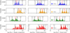 |
Fig. 3 Comparison of the H II, H I, and H2 masses for different architectures. The histograms are built using the MCMC draws for the whole sample. The vertical lines show the minima and maxima of the distributions (dashed lines), the quantiles at 15% and 85% (plain black lines), and the median value (plain red line). |
4.3 Molecular gas reservoirs
4.3.1 Matching the CO emission
In Fig. 5, we plot the predicted CO luminosities versus the measured values, for all architectures. In single component models, the emission of CO is underpredicted by a factor larger than three (0.5 dex) for 6 out of 15 detected galaxies. Multicomponent models, with one to four components, perform better at reproducing CO (12 out of 15 detections are well reproduced within 0.5 dex), but they still underestimate CO (by a factor of more than 3) in three detected galaxies. The multi-component models based on power-law distributions are the only models to predict CO emission in agreement (within 0.5 dex) with the observations, for all the galaxies of our sample.
This inability of the models with a few (1–4) components to match CO emission is also illustrated by the P(3σ) values for CO only, reported in Table A.3. For single component models, the P(3σ) obtained for CO are low (≤25%) for 7/15 galaxies detected in CO, and null in 4/15. The P(3σ) obtained using multi-component models are globally larger, but remain below 25% for 3/15 detections, and null for one galaxy. In other words, the tracers of the ionized and neutral gas are reproduced at the expense of CO.
We note that this underestimation of CO lines was not present in M20, despite their use of a similar single-component approach, because the CO emission was matched a posteriori by adjusting the depth (AV) of each model. While such an adjustment successfully allows for CO matching, it modifies a posteriori the solution, which may not match anymore the other ionized gas and PDR tracers. Here, on the other hand, we consider AV as a free parameter and attempt to fit all lines simultaneously during the MCMC sampling. Within our Bayesian framework, we find that matching all constraints, including CO, is impossible for models with only a few components. This result indicates that in some galaxies, the CO emission can only be matched by models accounting for numerous clouds or gas components. This is discussed further in Sect. 6.1.
4.3.2 CO-bright versus CO-dark molecular gas
While the global mass distribution associated with H II, H I, and H2 are not significantly sensitive to the choice of a given configuration (see Fig. 6), the amount of CO-dark versus CO-bright H2 predicted using different geometries may vary significantly. Using Eq. (3), we extracted the masses of H2 associated with C+, C0, and CO. The histograms obtained for the whole sample in each configuration are provided in Fig. 6. Qualitatively, the total H2 masses in our sample are dominated by H2 reservoirs associated with C+, and to a lesser extent with C0, while the reservoirs associated with CO are 2–4· orders of magnitude below.
In a more quantitative way, we examine in Fig. 7 the ratios of the total H2 mass (MH2,total) to CO-bright H2 mass (MH2,CO), shown as a histogram for the whole sample. On average, we find that the galaxies in our sample are completely dominated by the CO-dark H2 masses. The predicted total H2 masses are on average 100 to 106 times larger than the H2 masses associated with CO, in all architectures, although larger for single component models. Specifically, we find median total-to-CO-bright ratios of 104.5, 103.7, and 103.4 for single component models, multi-component models, and power law models, respectively. Those numbers indicate that, on average, nearly 100% of the H2 gas is CO-dark in our sample. This is linked to the selection of our sample, which consists of extremely CO-faint galaxies and galaxies in which CO is undetected. We find that the predicted fractions of CO-dark gas are at least of 70%, 37%, and 80% in single component models, multi-component models, and power law models, respectively.
In Fig. 8, we plot the total-to-CO-bright H2 mass ratio as a function of [C II]/CO for the three architectures. In M20, this mass ratio was found to tightly correlate with the [C II]/CO. Similarly, we find a tight correlation of MH2,total/MH2,CO with [C II]/CO for single component models (left panel). Our predictions are slightly shifted away from the relation of M20 because CO is underpredicted by single-component models, as already pointed out in Sect. 4.3.1. The correlation between MH2,total/MH2,CO and [C II]/CO still holds when a larger number of components are combined. Nevertheless, we find that increasing the number of components flattens the relation and increases its dispersion. Indeed, purely CO-dark components (corresponding either to diffuse CO-dark reservoirs or CO-dark clumps) may be included in the models when combining components. This is not the case with a single component model where the CO-dark H2 envelope is always associated with CO-bright H2 core. Hence, models combining components predict higher M(H2)total/M(H2)CO at fixed [C II]/CO (i.e., larger content of CO-dark gas), and a larger spread around the average linear relation.
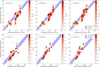 |
Fig. 4 Dust and H I masses predicted by single component (left), multi-component (middle), and power law models (right). The red points mark the location of robust means and the ellipses the 1σ uncertainty around the main peak, following the skewed uncertainty ellipses formalism described in Galliano et al. (2021). We report the mean and standard deviation of the Spearman correlation coefficients (ρ) calculated for of the whole sample, at each of the MCMC steps, represented by the shaded kernel density estimate underlying data points. The dashed lines indicate the 1:1 relation and the blue shaded area a deviation of 0.5 dex around the latter relation. |
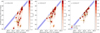 |
Fig. 5 Predicted vs. observed CO emission for single-sector model (left column), multi-sector models (middle column), and power law models (right column). The shades, symbols, and legends are described in Fig. 4. |
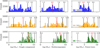 |
Fig. 6 Comparison of the M(H2)CO, M(H2)C and M(H2)C+ for different architectures. The histograms are built using the MCMC draws for the whole sample. The vertical lines show the minima and maxima of the distributions (dashed lines), the quantiles at 15% and 85% (plain black lines), and the median value (plain red line). |
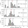 |
Fig. 7 Stacked histograms of the posterior distribution of the total-to-CO-bright H2 masses for the whole DGS sample. The histograms are built using the MCMC draws for the whole sample. The vertical lines show the minima and maxima of the distributions (dashed lines), the quantiles at 15% and 85% (plain black lines), and the median value (plain red line). |
5 Results using statistical distributions of the components
As discussed in Sect. 4.3.1, the architecture using power-law and broken power-law distributions for the U, n, and cut parameters performs better at reproducing the CO emission in our sample. We now focus only on the latter architecture to infer the integrated molecular gas masses and αCO values.
5.1 Constraints on the power laws and broken power laws
As described in Sect. 3.2.3, we combine components following power laws (defined by a slope over a given range of values between a lower and upper bound) for the density and ionization parameter and a broken power law (defined by two slopes over two ranges of values separated by a pivot point) for the cut parameter. We consider relatively weak priors for the slope and boundaries, defined as normal distributions centered on a value µ with a relatively large σ. We now examine the means of the posterior PDFs for the density, ionization parameter, and cut in our sample.
In Fig. 9, we show the means of the posterior PDFs obtained for the slopes and boundaries of the distributions for density, ionization parameter, and cut in each of the individual galaxies. We note that the power laws controlling the density and ionization parameter are parameterized using the values of U and n at the illuminated face of the clouds, which may differ from the volume-averaged U and n. In Table A.2, we report the luminosity weighted-averaged of the corresponding parameters: the density and the ionization parameter at the illuminated edge of H II regions, as well as the cuts in the ionized gas (#1) and neutral gas (#2).
On the left panel of Fig. 9, the mean slopes obtained for the distribution of density are all negative, meaning that components with relatively low density dominate the emission with respect to denser regions. As reported in Table A.2, the averaged densities in the H II regions are ~ 10–100 cm−3, which is close to the typical values often considered for H II regions in thermodynamic equilibrium. We note that three galaxies, NGC 1140, NGC 5253, and UM 448, have mean densities lower than 10 cm−3. We speculate that the relatively high contribution of low density gas in those galaxies may be due to a disturbed morphology of the gas (e.g., ionization cones in NGC 5253; Zastrow et al. 2011, interaction-induced inflow in a merger system for UM 448; James et al. 2013, complex ionized gas structure associated with superbubbles and shocked shells in NGC 1140; Westmoquette et al. 2010). On the other-hand, SBS 0335-052 is associated with a larger mean density value (~ 100 cm−3) than the other galaxies and a relatively high lower bound for the density (~67 cm−3), which suggests that diffuse regions do not contribute much to the observed emission in this galaxy. In the middle panel of Fig. 9, we observe mostly negative medians for the slopes of the distribution of ionization parameters, meaning that regions with relatively low ionization parameters may dominate the total luminosity in most galaxies. The range of slopes covered by the whole sample is large, with several galaxies showing relatively flat slopes and three galaxies with a positive slopes (i.e, dominated by components of high ionization parameters). The means reported in Table A.2 are between ~−3 and −1.5, with three galaxies associated with relatively higher ionization parameters (II Zw 40, Mrk 209, and SBS 0335-052) between −1.5 and −1.25.
In the right panel of Fig. 9, we plot the broken power-law parameters for the cuts, which show a change of slopes at the ionization front (cut=l). This drastic change of slope is indicative of the presence of different populations of gas components, depending on their optical depth. Specifically, we find that the distribution of “naked” H II regions, which are not associated with any neutral gas (i.e., cut ≤1), differs from the distribution of embedded H II regions associated with a complete or partial PDR, and potentially with molecular gas (i.e., cut >1). We observe a large spread in the slopes obtained for each individual galaxy, with both negative and positive slopes found in the ionized gas and in the neutral gas.
Interestingly, if we focus only on galaxies associated with the largest upper bounds for cuts (e.g., cut ≥ 2, indicating that the models include components that are deep enough to exceed the dissociation front), we find that they are all associated with clearly negative slopes for the cuts within the neutral gas. Qualitatively, such negative slopes indicate that the component with relatively smaller optical depths are more numerous and dominate the total luminosity, while fewer components reach greater optical depths contribute to the emission. These features could be associated with a “clumpy” distribution of dense clouds and will be further discussed in Sect. 6.1. In Table A.2, we identify in bold 6/18 galaxies associated with upper bounds higher than 2, which are further examined in Sect. 5.2.3. The averaged values for the cut in the ionized gas are always between 1 (ionization front) and 2 (dissociation front), which is indicative of galaxies dominated (in mass) by atomic neutral gas rather than molecular gas, as discussed in Sect. 4.2. The mean cut values in the ionized gas are between ~0.6 and ~0.8, while we may expect mean cut values closer to unity, if most of the H II regions were radiation-bounded. Such values may reflect an important contribution of density-bounded regions to the total luminosity. The presence of the latter regions, potentially associated with leakage of ionizing photons, was studied in more details in Ramambason et al. (2022).
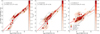 |
Fig. 8 MH2,total/MH2,CO versus [C II]/CO(l–0) for single component models (left), multi-component models (middle), and power law models (right). The shades and symbols are described in Fig. 4. The dashed gray lines corresponds to the relation from M2O while the dashed red lines show the linear regressions fitted to the combined posterior distribution for the entire sample. We indicate the equations of linear regressions fitted to the 2D-PDF of the whole sample and the associated coefficients of determination R2. |
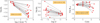 |
Fig. 9 Values of the power-law parameters for individual galaxies controlling the density (left), ionization parameter (middle), and cut (right) for each galaxy. The red dots correspond to the means of the lower and upper boundaries of power laws (and pivot point for the broken power law) and the gray lines represent the power laws corresponding to the averages slope values, for each galaxy. |
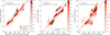 |
Fig. 10 Predicted line fluxes for [C II] [C I], and CO emission lines vs. MH2,total for multi-component models with power-law distributions. The predictions for [C II] and CO match well the observed measurements, as shown in Figs. A.3 and 5. The predictions for [C I] are purely model-based, since no measurement is available. The dashed gray lines show the relations from M20 while the dashed red lines show the linear regressions fitted to the combined posterior distribution for the entire sample. The shades, symbols, and legends are described in Fig. 4. We indicate the equations of linear regressions fitted to the 2D-PDF of the whole sample, and the associated coefficients of determination R2. |
5.2 Total H2 masses
5.2.1 Tracers of M(H2)
In Fig. 10, we plot the evolution of the total H2 masses predicted by the power law models with respect to different tracers: [C II], [C I], and CO(1–0). All the galaxies are detected in [C II] and our line flux predictions are in excellent agreement with the observed values as shown in Fig. A.3. For [C I], our plots show purely predicted luminosities since no detection is available in our sample. Nevertheless, as discussed in Sect. 4.3.1, the power law models are in good agreement with the few tracers arising from the PDRs, as shown by the P(3σ) in Table A.3 and in Fig. A.3. For the CO(1–0), our predictions are in good agreement within 0.5 dex with all measurements, as shown in Fig. 5.
We find that the total H2 mass correlates best with [C II]158 µm, with a Spearman coefficient of 0.92 ± 0.03. As shown in the left panel of Fig. 10, the relation we derive is slightly below that of M20. This systematic offset comes from the nature of the power law models (see Sect. 4.3.1), which allows us to match the CO emission with numerous components rather than assuming a single component. As a result, the total H2 masses derived for a fixed [C II] value are systematically smaller than those derived in M20, on average by a factor 180. We note that the single component models (presented in Sect. 3.2.1), predict masses in perfect agreement with the M20 relation, indicating that this offset is merely due to the different distribution of gas (i.e., more independent components) considered in the multi-component models.
In the middle panel of Fig. 10, we show the relation between H2 mass and [C I] 609 µm. We find that based on our predictions, [C I] 609 µm also provides an excellent tracer of the total H2 (with a Spearman correlation coefficient of 0.9 ± 0.03), although with a slightly larger dispersion than for the [C II] line. We predict a shallower relation than that derived in M20 based on single-sector models with a fixed metallicity of 1/10 Z⊙. On the right panel of Fig. 10, we show the relation between M(H2) and CO(1–0). Although the two quantities are correlated, we find a lower Spearman correlation coefficient (ρ = 0.8 ± 0.07) and a lower regression coefficient than for [C II] and [C I]. Our predictions suggest that both [C II] and [C I] are better tracers of the total H2 mass than CO(1–0) at low metallicity and should be preferred, provided that they can be detected.
5.2.2 Conversion factors
In Fig. 11, we translate the relations from Sect. 5.2.1 into conversion factors, assuming that the area of emission is the same for all tracers5. We then examine the variations on those conversion factors with metallicity. As shown in Fig. 11 (left and middle panel), we find a nearly constant α[CII] value at all metallicities while the α[CI] values anticorrelate with metallicity, with a slope close to −1. We note, however, that there is a significant scatter (~2 dex) around both relations, which is linked to the variety of gas geometry considered when combining many components. We find similar trends of α[CII] and α[CI] values with metallicity when considering lower numbers of components (from one to four components; see Sects. 3.2.1 and 3.2.2), with an increasing scatter as a function of the number of components.
Despite the large scatter, α[CI] (middle panel) shows a clear metallicity trend, with a Spearman coefficient of −0.45 ± 0.12. We derived a negative slope of −1.39, which is in relatively good agreement, although slightly steeper, with the slopes derived in both observational and theoretical studies. In particular, our predictions are compatible with the study from Heintz & Watson (2020), which derived a slope of −1.13 based on samples of high-redshift γ-ray burst and quasar molecular gas absorbers. The slope we derive is also close to the value of about −1 derived by Glover & Clark (2016) based on simulations of star forming clouds, just before the onset of star formation. The latter study also points out that the exact dependence of α[CI] with metallicity is sensitive to dynamical effects and is likely to vary over time. Those effects are ignored in our stationary 1D models and will be further discussed in Sect. 6.2.
Finally, we examine the αCO versus metallicity dependence, shown in the right panel of Fig. 11. While we observe a clear dependence of αCO with metallicity, we find a relatively low absolute value for the Spearman correlation (0.19), indicating that the monotonic trend is weak. This is especially striking when compared to the results from M20 for which the αCO of the DGS galaxies followed a steep relation with metallicity with a narrow dispersion (0.32 dex). Instead, we find a large scatter at fixed metallicity for the power law models, which match best the observed emission lines (see Sect. 4.3.1). While most of the galaxies in our sample are found to be in good agreement with the steep relation from M20 and Schruba et al. (2012) and several αCO values are in better agreement with flatter relations (e.g., Amorín et al. 2016; Accurso et al. 2017), while three galaxies have a predicted αCO values close to the Galactic value (within a factor of 3 based on their 1σ uncertainties), despite their subsolar metallicity. This finding indicates that the αCO may be driven by another physical parameter. In the next section, we further explore the impact of the geometry of our models on the derived αCO values, through the clumpiness of the gas.
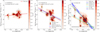 |
Fig. 11 αCII (left), αCI (middle), αCO (right) versus metallicity for power law models. The shades, symbols, and legends are described in Fig. 4. We indicate the equations of linear regressions fitted to the 2D-PDF of the whole sample, and the associated coefficients of determination R2. We also show the Galactic αCO value from B13 and the range of values compatible with it within 30% (gray-shaded area), the αCO vs. metallicity relations from M20, Schruba et al. (2012), Amorín et al. (2016), and Accurso et al. (2017), and the α[CI] vs. metallicity relations from Glover & Clark (2016) and Heintz & Watson (2020). We use a Galactic conversion factor of 3.2 M⊙ pc−2(K km s−1)−1 to correct for the helium mass (factor of 1.36) when comparing to the model prediction of M(H2). |
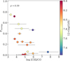 |
Fig. 12 Clumpiness parameter (defined by Eq. (11)) vs. predicted [C II]/CO ratio, colorcoded as a function of metallicity. The clumpiness parameter is anti-correlated with the [C II]/CO ratio and has a secondary dependence with metallicity. |
5.2.3 Impact of clumpiness on αCO
To further examine the different morphologies of galaxies inferred by our code, we define a “clumpiness” probability parameter as follows:
 (11)
(11)
where < C > is the averaged value of the posterior PDF of the binary variable C, αcut,2, and cutmax are respectively the slope and upper-bound of the distribution followed by the cut parameters (see Sect. 3.2.3).
The introduction of the clumpiness parameter allows us to qualitatively define two morphologies of CO-bright molecular gas: 1) diffuse CO distribution, corresponding to low Pclumpy parameters, in which the CO emission is dominated by numerous low-AV clouds6. The inferred distributions favor low upper-bounds (cutmax < 2) meaning that most clouds do not reach their dissociation front, and positive slopes, corresponding to relatively larger contribution of such clouds, with respect to deeper clouds, to the total gas mass; 2) clumpy CO distribution, corresponding to large Pclumpy parameters, in which the CO emission is dominated by a few high-AV clouds. In such galaxies, the distribution of parameters inferred by our models favors large upper-bounds (cut > 2, meaning that some regions drawn during the sampling reach large AV, after the dissociation front) and negative slopes (αcut,2 < 0), meaning that such deep clouds with large AV contribute relatively less to the total gas mass than the lower-AV components. As the Pclumpy parameter increases, galaxies gradually evolve from a diffuse CO distribution to a clumpy distribution.
In Fig. 12, we show the variation of the clumpiness parameter, Pclumpy, as a function of the predicted luminosity ratio [C II]/CO and find a relatively strong anti-correlation with a Spearman correlation coefficient of −0.59. This relation appears to shift with metallicity, with lower metallicities being associated with larger clumpiness parameter at fixed [C II]/CO ratio. In Fig. 13, we then examine how the clumpiness parameter relates to αCO and the metallicity. In the left panel, we see that the dispersion in the αCO versus the metallicity relation is mainly linked to the clumpiness parameters. Galaxies corresponding to the diffuse CO distribution, with Pclumpy ≲ 0.4 are close to the steep relations from Schruba et al. (2012) and M20. On the contrary, the clumpiest galaxies with Pclumpy ≳ 0.4 deviate significantly from the latter relations and are associated with lower αCO. The latter galaxies are flagged in bold in Table A.2.
In the right panel of Fig. 13, we show αCO versus Pclumpy which exhibits a clearer anti-correlation than the αCO vs. metallicity, with a Spearman coefficient of −0.51. In particular, the three clumpiest galaxies (Pclumpy > 0.5) in our sample are found close to the Galactic αCO (within a factor of 3), despite their subsolar metallicities. While one of them, He 2–10, has the highest metallicity in our sample (12 + log(O/H) = 8.43 ± 0.01, Madden et al. 2013), the two other clumpiest galaxies, Mrk 209 and UM 461, both have a metallicity close to ~1/10 Z⊙ (respectively, 12 + log(O/H) = 7.74 ± 0.01 and 12 + log(O/H) = 7.73 ± 0.01; Madden et al. 2013).
Nevertheless, we still find that metallicity plays an important role, with the two lowest metallicity galaxies, I Zw 18 and SBS 0335-052, being clearly offset toward larger αCO. The αCO variations can be relatively well described by fitting a simple linear relation, which depends on both the metallicity and clumpiness parameter:
 (12)
(12)
where Z is the metallicity given as 12 + log(O/H), Pclumpy the clumpiness parameters (see Eq. (11)), and with an optimal slope of β = −3.51 ± 5 × 10⁻⁵. In the latter equation, the clumpiness parameter modulates the slope of the αCO versus metallicity anticorrelation that flattens with increasing clumpiness. For Pclumpy=0, we find a slope of −3.51 which is close to that of M20 (−3.39). We argue that the M20 relation, derived assuming a diffuse CO emission provides an upper limit on αCO while the actual αCO accounting for the clumpiness of the medium, decreases with increasing Pclumpy. We further discuss the possible physical mechanisms leading to either a clumpy or diffuse distribution of molecular gas in Sect. 6.1.
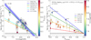 |
Fig. 13 Relation between the αCO vs. the gas-phase metallicity (left panel) and the clumpiness parameter (right panel), defined by Eq. (11). The Spearman correlation coefficients are calculated for the means of individual galaxies, shown by colored dots. We show the Galactic αCO value from B13 and the range of values compatible with it within 30% (gray-shaded area). |
6 Discussion
6.1 Clumpy versus diffuse molecular gas at low metallicity
6.1.1 Geometry of the cold ISM at low metallicity
The current study is aimed at recovering information about the mass distribution of CO-emitting clouds in spatially unresolved galaxies. We introduced multi-component models (described in Sect. 3.2.3) that provide luminosity-weighted predictions for emission lines and masses, accounting for the relative contribution of diffuse low-AV clouds versus denser larger-AV clouds (see Sect. 5.2.3). Our sample of dwarf galaxies (see Sect. 2.1) is best fitted by different luminosity-weighted topologies, going from a diffuse CO distribution (dominated by many low-AV clouds) to a clumpy CO distribution (dominated by a few high-AV clouds). Most of the DGS galaxies (12 out of 18 in this study) are associated with a “diffuse” scenario which matches the picture drawn from previous works of substantial CO-dark molecular gas reservoirs and large αCO values in low-metallicity environments (e.g., Lebouteiller et al. 2017, 2019; Chevance et al. 2020; Madden et al. 2020). Nevertheless, our results predict that a clumpy molecular gas geometry (Pclumpy ≥ 0.4) is expected for 6 out of 18 galaxies in our sample.
Such results are consistent with recent observations, performed at high spatial resolution with ALMA, which have revealed CO clumps with sizes of 10–100 pc in several of the galaxies included in the current study (e.g., NGC 625 at ~20 pc resolution; Imara et al. 2020, II Zw 40 at ~24 pc resolution; Kepley et al. 2016, He 2–10 ~26 pc resolution; Imara & Faesi 2019). Among the three clumpiest galaxies identified in our study, He 2–10 is associated with a high Pclumpy of 0.75, which is consistent with the observations from Imara & Faesi (2019), which reported the presence of 119 resolved giant molecular clouds, with average sizes of ~26 pc in which 45–70% of the total molecular mass is concentrated. The authors report a CO-to-H2 conversion factor of 0.5 to 13 times the Milky-Way value, which is also in good agreement with our predictions. The two other clumpiest galaxies identified by our models (UM 461 and Mrk 209) have not been mapped in CO at high resolution. It is also possible that CO resides in even smaller clumps (≲ 10 pc), below the resolution of the existing ALMA observations. Indeed, recent observations performed at very high-angular resolution in other low metallicity dwarf galaxies have detected CO-clumps with sizes as small as a few parsecs (e.g., Oey et al. 2017; Shi et al. 2020; Schruba et al. 2017; Rubio et al. 2015; Archer et al. 2022). In the Magellanic Clouds, recent studies have shown that CO emission has a complex, highly filamentary structure both in the LMC (Wong et al. 2019, 2022) and in the SMC (Ohno et al. 2023), and have identified CO sub-structures with equivalent radius down to ~0.1 pc.
Nevertheless, the latter observations remain scarce and were performed at different spatial resolutions. Observing a representative sample of dwarf galaxies at high spatial resolution is needed to perform a meaningful comparison with the clumpiness predictions from the current study and to better understand the physical and chemical mechanisms driving the clumpiness of molecular gas in the ISM. Meanwhile, magnetohydrodynamical (MHD) simulations may help to gain insight into the structures that may form in cold neutral gas. In a recent work simulating galaxies with metallicities ranging from 0.2 to 1 Z⊙, Kobayashi et al. (2023) reported the presence of small cold neutral medium structures with sizes ~0.1–1 pc, which form naturally out of converging gas flows, although over longer formation timescales at lower metallicity. Regardless of their exact sizes, our results suggest that clumps may dominate the integrated CO luminosity, with important implications on the integrated gas masses and on the star formation laws derived at galactic-scales.
6.1.2 Impact of clumpiness on integrated gas masses and αCO conversion factors
As discussed in Sect. 4.2, changes in terms of gas topologies (i.e., number and distribution of components) have little effect on the predicted values for the total gas masses associated with the ionized, neutral, and molecular gas reservoirs (see Fig. 3). However, the topology of our models strongly affects how H2 is distributed between the warm CO-dark phase (associated with C+ and C0) and the cold CO-bright phase (associated with CO, see Figs. 6 and 7). While the DGS galaxies are found to be largely dominated by CO-dark H2, regardless of the architecture, we show that single-component models and models with only a few components tend to overestimate both the fractions of CO-dark H2 gas (see Fig. 7) and the total integrated H2 mass (see Fig. 10).
Using statistical distributions of components to mimic a clumpy medium, we find that all the galaxies in our sample are H I-dominated, with M(H2)/M(H I) ranging from ~5% to 66% (see Sect. 4.1). This result differs from those of Cormier et al. (2014), which predict several H2-dominated galaxies using the same sample, based on an αCO prescription that scales with metallicity. Our predictions are in better agreement with the global mass distributions observed in larger surveys, such as the xGASS survey. In the latter survey, the atomic gas fractions are found to increase with decreasing stellar masses, leading to an average M(H2)/M(H I) ratio close to 10% for stellar masses of ~109 M⊙ (Catinella et al. 2018).
We find a large dispersion around the αCO versus metallicity relation (see Fig. 11), which we interpret in terms of clumpiness of the medium (see Fig. 13). The clumpiness parameter, defined by Eq. (11), anti-correlates with the [C II]/CO emission line ratio, as shown in Fig. 12. In other words, our results recover the variations of αCO as a function of [C II]/CO, observed in large samples of galaxies up to ɀ ~ 2.5 (Accurso et al. 2017), and provide a new physical interpretation in terms of clumpiness of the ISM. Our predicted αCO values are anti-correlated with both the metallicity and clumpiness, and are well described by a linear equation involving both parameters (see Eq. (12)). As a result, low-metallicity galaxies may be associated with low αCO values, close to the Galactic value, provided that they have a clumpy molecular gas distribution.
This finding is in line with results from Gratier et al. (2017) in the small spiral galaxy M33 that report an average αCO of twice the Galactic value, despite its half-solar metallicity. Similarly, αCO values of less than a factor ten larger than the Milky-Way value were reported in the Large and Small Magellanic clouds despite their subsolar metallicities (Pineda et al. 2017; Jameson et al. 2018; Saldaño et al. 2023). In particular, Pineda et al. (2017) find that accounting for the small filling factor of CO emission tends to reduce the derived αCO values.
A complementary picture is provided in Hu et al. (2022) that couple hydrodynamical simulations with time-dependent H2 chemistry to study the effect of metallicity variations on the αCO derived from post-processed CO maps. The authors report significant spatial variations of αCO on parsec scales, with diffuse clouds being associated with high αCO values, while denser clouds, from where CO mainly arise, are associated with low αCO values. To account for those spatial variations, Hu et al. (2022) introduce a multivariate αCO calibration that is not only a function of metallicity, but also depends on the beam size and line intensity.
6.1.3 Impact on star-formation laws
While a few studies have examined the atomic gas-to-SFR relation in H I-dominated dwarf galaxies (see e.g., Bigiel et al. 2008), estimates of their total molecular gas surface density, including H2, have remained challenging. An unprecedentedly large sample of dwarf galaxies is included in the recent analysis of de los Reyes & Kennicutt (2019) that revisit the integrated KS law in a wide range of environments, but the authors specifically excluded the blue compact dwarf galaxies (BCD), which are similar to the galaxies in our sample, to focus on non-starbursting systems. In a subsequent paper, Kennicutt & De Los Reyes (2021) provided an updated version of the KS law for spiral and starburst galaxies including BCDs, but most of their sample consists of massive galaxies. In addition, the necessity to adopt of a CO-to-H2 conversion factor to estimate the total molecular gas surface density yields large uncertainties, especially for low-metallicity galaxies. Hence, it remains unclear whether star-forming dwarf galaxies are expected to follow the classical KS law, and predictions based on simulations (such as e.g., Whitworth et al. 2022) or models such as Cormier et al. 2014 or M20 are much needed.
We translate the predicted H I and H2 masses inferred by the power law models into gas surface densities to examine the starformation laws in the DGS. As previously done in Cormier et al. (2014) and M20, we use the dust photometric apertures reported in Rémy-Ruyer et al. (2015) to estimate the angular size of the emission. We note that the predicted H I masses are globally in good agreement with the available measurements based on 21 cm emission (as shown in Fig. 4). The measured H I masses were corrected so that they correspond to the exact same photometric apertures as the integrated line fluxes used in our modeling. This correction was performed by estimating the total H I-emitting area and assuming a Gaussian distribution profile of the H I 21 cm emission. We stress that the uncertainties on the latter corrections remain quite large and the Gaussian profile adopted to model the H I radial extent may overestimate the amount of H I located within the photometric aperture, meaning that H I masses could be overestimated both in models and in observations. We assumed that both H2 masses and the corrected H I masses broadly correspond to the same spatial area and derived an average gas surface densities over the dust apertures. In practice, the latter aperture may lead to an overestimation of Σ(H I), although this is mitigated by the correction of H I masses, and to an underestimation of Σ(H2), especially since H2 clumps may have sizes much smaller than the photometric apertures (~ 1–500 kpc2).
Despite these uncertainties, we examined the position of our sample of star-forming low-metallicity dwarf galaxies with respect to classical star-formation laws in starbursting and non-starbursting galaxies. Figure 14 shows that the DGS galaxies are globally in good agreement with the star formation law derived in Kennicutt & De Los Reyes (2021) for an extended sample of starbursting galaxies and spiral. As previously reported in M20, accounting for the CO-dark H2 gas solves the apparent offset of dwarf galaxies, which appear shifted toward lower gas surface densities when accounting only for the CO-bright H2 gas (e.g., Cormier et al. 2014). For the “clumpy” subsample of galaxies we derive a nearly linear relation corresponding to a constant depletion time of ~1 Gyr. Despite low statistics leading to large uncertainties on the fit, we find that the relation we derived for clumpy dwarf galaxies is compatible with the classical KS law derived for more massive for spiral and starburst galaxies in Kennicutt & De Los Reyes (2021).
On the other hand, we find that several galaxies among the ones predicted to have a diffuse CO distribution are offset toward large gas surface densities and correspond to higher depletion times, between 1 to 10 Gyrs. While similarly long depletion times have been reported for H I-dominated irregular dwarf galaxies in Bigiel et al. (2008) and for non-starbursting dwarf galaxies (see e.g., the low surface density galaxies and faint irregular dwarf galaxies from Wyder et al. 2009 and Roychowdhury et al. 2017 shown in de los Reyes & Kennicutt 2019), the latter timescales appear surprisingly large for star-bursting galaxies. Galaxies associated with large depletion times (5 out of 18 galaxies with depletion time > 1 Gyr) are responsible for a flattening of the slope that we derive, leading to a sublinear relation (slope of 0.59 ± 0.28) for dwarf galaxies with diffuse CO distribution. The latter relation is incompatible with the classical KS law for more massive starbursts, even within the large fit uncertainties. We speculate that this offset may be linked to the presence of diffuse molecular gas reservoirs that are not associated with any star forming regions, an explanation that was previously invoked in Shetty et al. (2013,2014) to account for the flattening of the KS. In particular, Shetty et al. (2014) claimed that the fraction of diffuse, non-starforming CO-bright component could be at least of 30% in extragalactic observations. The presence of a diffuse gas reservoir, shining in CO, is qualitatively consistent with our results and the fact that most galaxies in our sample (12 out of 18) are associated with relatively low clumpiness parameters.
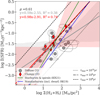 |
Fig. 14 ΣSFR vs. Σ(H2+H I). The galaxies associated with a “clumpy CO” distribution are reported in bold in Table A.2 and correspond to Pclumpy ≥ 0.4 (see Eq. (11)), while the others correspond to a “diffuse CO” distribution. Plain lines correspond to the best fits obtained for those two categories, with their 95% confidence intervals shown as shaded-areas, as well as the relations derived for starbursting galaxies and non-starbursting galaxies from Kennicutt & De Los Reyes (2021) and de los Reyes & Kennicutt (2019), respectively. |
6.2 Known caveats and potential improvements
6.2.1 Limitations of the SFGX grid
While the statistical framework provided by MULTIGRIS allows us to consider complex, more realistic geometries of the gas, its accuracy ultimately depends on the underlying grid of 1D models. In the current study, we used the SFGX grid (see Sect. 3) composed of spherical Cloudy models, computed at thermal equilibrium. A first caveat, already mentioned in Sect. 2.2 is that the radial sampling of our grid does not enable to properly capture the sharp increase of H2 cumulative emission (as shown in Fig. A.1). Mid-IR H2 upper limits are overpredicted by our models, especially for the two lowest levels (H2 S(0) and H2 S(1)). This problem is somewhat mitigated for the detections, which are found in relatively good agreement with predictions, but also tend to be overpredicted for H2 S(0) and H2 S(1). While this issue is restricted only to H2 lines, associated with a sharp radial increase of the emission, it prevents us from using H2 lines as constraints. The latter H2 lines would provide additional information on the neutral atomic and molecular gas phase, for which few tracers are available (see Table 2). While resampling the grid using a finer step in cut or interpolating between different cut values may improve the solutions, properly recovering the fluxes of tracers with sharp radial variations remains challenging with our method. Carefully selecting the list of lines used in the analysis and excluding the problematic tracers remains, for now, the best option.
A second caveat is that Cloudy models are static, while time-dependent effects have been shown to strongly affect both H2 predictions and the associated CO-to-H2 conversion factors (e.g., Glover & Clark 2012b). Specifically, Hu et al. (2021) show that steady-state models tend to overestimate H2 and the CO-dark gas fraction with respect to time-dependent models. As a result, Hu et al. (2022) found that the CO-to-H2 conversion factors derived using time-dependent models are systematically lower than those derived using steady-state models. Based on a highly-resolved (~0.2 pc) ISM simulation of an isolated low-metallicity (1/10 Z⊙) dwarf galaxy post-processed using a time-dependent chemistry network and a dust-evolution model, Hu et al. (2023) recently derive a CO-to-H2 conversion factor close to the Milky-Way value. Accounting for out-of-equilibrium chemistry may result in even lower αCO values than those predicted in the current study.
Additionally, several physical quantities are fixed in the SFGX grid, some of which may be important in order to correctly predict the emission in the neutral and molecular gas. First, the adopted cosmic ray ionization rate (CRIR) is an important parameter to accurately predict CO. The effect of an enhanced CRIR on the CO emission is not trivial as it depends on the density: at low densities ( n ~ 102 cm−3), it causes a decrease in CO emissivity, while at higher densities, this effect is compensated by the rise in temperature (e.g., Bisbas et al. 2015; Vallini et al. 2019). Based on MHD simulations, Gong et al. (2020) found that a decrease of αCO is expected at higher CRIR. In the current study, we follow the prescription of Cormier et al. (2019) and adopted a CRIR value that is about three times higher than the standard Galactic value from Indriolo et al. (2007) in order to account for the recent star-formation history in the DGS. This value remains somewhat arbitrary and is not varied in the SFGX grid. Nevertheless, the SFGX grid includes a variable contribution from X-ray sources with luminosities ranging from 0 to 10% of the stellar luminosity, which may match the emission of galaxies with higher CRIR than the one considered in our models. We note that cosmic rays and X-rays have similar effects in terms of ionization and heating on the PDR tracers (e.g., Lebouteiller et al. 2017); hence, their effects cannot be disentangled with our set of constraints, which include only one line arising from the molecular gas. Disentangling the complex effects of enhanced CRIR and X-rays would require constraining the entire CO-sled (e.g., Vallini et al. 2019; Esposito et al. 2022), which is not possible with only CO(1–0).
Finally, as mentioned in Sect. 3.1.3, the radial density profile in our Cloudy models follows a physically motivated prescription introduced in Cormier et al. (2019), with density increasing linearly in the dense gas, above a given density threshold. This law controls the density profile of the PDR and molecular clouds associated with H2 regions, and directly impacts the luminosity and mass estimates that we derive. The effect of choosing a different density law was examined in Cormier et al. (2019) which tried to fit constant pressure and constant density models to the DGS galaxies. They found that some variations are expected, in particular for [O I] lines, for which the emission is boosted in constant pressure models and decreased in constant density models. Nevertheless, the authors report that such changes did not significantly affect the quality of their fits. The effect of changing density laws is not examined in the current study as it would require running numerous additional Cloudy models, and because it is not clear that this could be constrained within our multi-component framework. Nevertheless, we point out that changing this prescription would likely change the distribution of parameters and the gas geometry inferred by our multi-component models.
6.2.2 Improving the statistical distributions
In Sect. 3.2.3, we present combinations of models based on the use of power laws and broken power laws to describe three main parameters in the study: the density, n, the ionization parameter, U, and the radial depth controlled by the cut. While the use of power laws to describe the distribution of such parameter is physically motivated, other PDFs could be considered based on the information provided by both theoretical studies and resolved observations.
In particular, the expected shape of the density PDF has been examined in several theoretical works. In a gravoturbulent ISM, the density of the gas is expected to follow a log-normal distribution at low densities (associated with a turbulent-dominated regime), while the high-density region is well-described by a power law, associated with a self-gravity dominated regime (e.g., Offner et al. 2014; Burkhart 2018; Burkhart & Mocz 2019; Jaupart & Chabrier 2020; Appel et al. 2023). Hence, the power-law distribution adopted in this study is well-suited to describe the dense star-forming gas but may break down at lower density, where turbulence plays an important role. A possible improvement of the models would be to include a log-normal distribution to account for the diffuse ISM component. Nevertheless, we note that the exact transition between the turbulent-dominated and gravity-dominated regimes is not well-known (e.g., at the location of shock fronts; Appel et al. 2023, at the phase transition between ionized and neutral gas, or between a cold and warm neutral medium; Kobayashi et al. 2022) and the transition point should be considered as an additional free parameter.
The power-law distribution adopted for the ionization parameter is even less easily constrained. In the current study, we use the ionization parameter at the illuminated front as a proxy to control the intensity of the radiation fields. While the ionization parameter provides a convenient proxy to parameterize models, it can be defined differently (either at fixed radius or as a volumic average) and has known dependencies on several other parameters such as metallicity, stellar mass, and the spatial scales (e.g., Ji & Yan 2022). Deriving meaningful priors for the ionization parameter, based either on observations or simulations, may not be straightforward.
A similar issue arises from the use of distribution of cuts rather than a parameterization based on the visual extinction, AV, or on column densities. While the cut parameter allows us to consider different distributions in the ionized gas and in the neutral gas, it prevents any direct comparison among the inferred geometries and the observation or simulations. The clumpiness parameter (introduced in Sect. 5.2.3) cannot be used outside the framework of this study. A more physically motivated approach would consist in describing models based on either on column density of molecular clouds or on AV-PDFs, as, for example in Bisbas et al. (2019, 2023). Even with those quantities, the analytical functions remain debated (e.g., lognormal as in Bisbas et al. 2019, 2023 or power laws as in Brunt 2015; Lombardi et al. 2015). Observational biases such as resolution, noise, boundaries, and superposition effects may also distort the true underlying PDFs of physical parameters, as discussed for example in Lombardi et al. (2015).
Finally, while we have focused on refining the combination of gas parameters, the exploration of the parameter space associated with the stellar population and X-ray sources is beyond the scope of the current study. Nevertheless, the distributions of parameters accounting for the spread in age and luminosity of the population of stellar clusters, as well as the effect of X-ray sources illuminating parts of the gas reservoirs, should also be explored. At any rate, statistics on the population of resolved H II regions or on the stellar cluster distributions based on high angular resolution observations (e.g., with MUSE or JWST) in combination with predictions from high-resolution simulations of galaxies are needed to introduce physically motivated priors on physical parameters.
7 Conclusion
In the current study, we revisit the results from M20 motivated by the extreme [C II]/CO(1–0) values observed in low-metallicity galaxies. We provide new predictions based on updated models and using a Bayesian statistical framework to account for the potentially complex structure of the neutral gas, through the use of statistical distribution of gas components. While the [C II]/CO variations were interpreted as changes in the visual extinction, AV, in M20, we find instead that the latter variations result from the combined effects of both the metallicity and the clumpiness of the ISM. Our main conclusions are summarized below:
Models combining numerous components based on statistical distributions of parameters are the only models able to match simultaneously the suite of ISM tracers used in our study, in all the galaxies of our sample. Models based on a combination of a few components (1–4) significantly underpredict CO(1–0) in at least 3 out of 18 galaxies;
Models combining a few components systematically overestimate the total H2 mass. When more components are considered, we find that all the galaxies in our sample are H I-dominated, which was not the case in previous studies;
Regardless of the modeling architecture, we find that H2 mass is always dominated by the reservoirs associated with C+, as well as C0 to a lesser extent, while the H2 masses associated with CO are negligible. This leads to large predicted fractions of CO-dark H2 gas in all galaxies, above 80% for models based on statistical distributions;
We confirm that [C II]158 µm is a good tracer of the total H2 mass and that α[CII] does not depend on metallicity. We derive a [C II] luminosity versus M(H2) relation, with a slope close to that of M20 but with a systematic offset toward lower H2 masses (a factor ~180 lower);
Our models predict that [C I]609 µm would also be a good tracer of the total H2 mass, although α[CI] is metallicity-dependent. We find a large scatter around the α[CII], α[CI], and αCO versus metallicity relations, associated with variations in the geometry of multi-component models;
We find that CO(1–0) is not a good tracer of the total H2 mass at low metallicity and that αCO strongly depends on both the metallicity and the clumpiness of the medium;
We find that the αCO versus metallicity relation derived in M20, assuming a simpler geometry for the models, only provides an upper limit on the actual αCO. While most of the galaxies in our sample (12 out of 18) are associated with a diffuse CO distribution and align on the M20 relation, we predict a clumpy geometry of CO-emitting clouds associated with reduced αCO values in 6 out of 18 galaxies. Two out of these six clumpy galaxies are predicted with αCO values ≤ 3 times the Galactic value, indicating that αCO may reach values close to the Galactic αCO regardless of the metallicity of the galaxy.
Acknowledgements
The authors thank the anonymous referee for constructive feedback and useful comments. L.R. and M.C. gratefully acknowledge funding from the DFG through an Emmy Noether Research Group (grant number CH2137/1-1). V.L., C.R. and L.R. thank the Transatlantic Partnership Program (grant number TJF21_053). COOL Research DAO is a Decentralized Autonomous Organization supporting research in astrophysics aimed at uncovering our cosmic origins. C.R. acknowledges the support of the Elon University Japheth E. Rawls Professorship.
Appendix A Additional figures
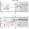 |
Fig. A.1 Cumulative emission lines profiles of some chosen tracers, including the H2 lines for the two models described in Figures 2 and 1. |
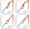 |
Fig. A.2 Predicted versus observed H2 lines for power law models. |
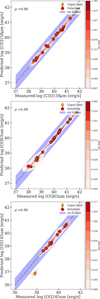 |
Fig. A.3 Predicted versus observed PDR lines for power law models. |
Best configuration selected for multi-component modeling with 1–4 components.
Luminosity weighted-averaged and slopes of the U, n, and cut1 (ionized gas), and cut2 (neutral gas) parameters of the power law models.
P(3σ) probabilities and averaged p-values for the power law models, multi-component, and single component.
References
- Accurso, G., Saintonge, A., Catinella, B., et al. 2017, MNRAS, 470, 4750 [NASA ADS] [Google Scholar]
- Ackermann, M., Ajello, M., Allafort, A., et al. 2012, ApJ, 755, 22 [NASA ADS] [CrossRef] [Google Scholar]
- Allen, R. J., Hogg, D. E., & Engelke, P. D. 2015, AJ, 149, 123 [NASA ADS] [CrossRef] [Google Scholar]
- Amorín, R., Muñoz-Tuñón, C., Aguerri, J. A. L., & Planesas, P. 2016, A&A, 588, A23 [NASA ADS] [CrossRef] [EDP Sciences] [Google Scholar]
- Appel, S. M., Burkhart, B., Semenov, V. A., et al. 2023, ApJ, 954, 93 [NASA ADS] [CrossRef] [Google Scholar]
- Archer, H. N., Hunter, D. A., Elmegreen, B. G., et al. 2022, AJ, 163, 141 [NASA ADS] [CrossRef] [Google Scholar]
- Asplund, M., Grevesse, N., Sauval, A. J., & Scott, P. 2009, ARA&A, 47, 481 [NASA ADS] [CrossRef] [Google Scholar]
- Baldwin, J., Ferland, G., Korista, K., & Verner, D. 1995, ApJ, 455, L119 [NASA ADS] [Google Scholar]
- Béthermin, M., Dessauges-Zavadsky, M., Faisst, A. L., et al. 2020, The Messenger, 180, 31 [Google Scholar]
- Bigiel, F., Leroy, A., Walter, F., et al. 2008, AJ, 136, 2846 [NASA ADS] [CrossRef] [Google Scholar]
- Bisbas, T. G., Papadopoulos, P. P., & Viti, S. 2015, ApJ, 803, 37 [NASA ADS] [CrossRef] [Google Scholar]
- Bisbas, T. G., Schruba, A., & van Dishoeck, E. F. 2019, MNRAS, 485, 3097 [NASA ADS] [Google Scholar]
- Bisbas, T. G., Tan, J. C., & Tanaka, K. E. I. 2021, MNRAS, 502, 2701 [CrossRef] [Google Scholar]
- Bisbas, T. G., van Dishoeck, E. F., Hu, C.-Y., & Schruba, A. 2023, MNRAS, 519, 729 [Google Scholar]
- Bolatto, A. D., Wolfire, M., & Leroy, A. K. 2013, ARA&A, 51, 207 [CrossRef] [Google Scholar]
- Boogaard, L. A., Decarli, R., Walter, F., et al. 2023, ApJ, 945, 111 [NASA ADS] [CrossRef] [Google Scholar]
- Braine, J., Gratier, P., Kramer, C., et al. 2010, A&A, 518, A69 [Google Scholar]
- Brunt, C. M. 2015, MNRAS, 449, 4465 [NASA ADS] [CrossRef] [Google Scholar]
- Burkhart, B. 2018, ApJ, 863, 118 [CrossRef] [Google Scholar]
- Burkhart, B., & Mocz, P. 2019, ApJ, 879, 129 [NASA ADS] [CrossRef] [Google Scholar]
- Catinella, B., Saintonge, A., Janowiecki, S., et al. 2018, MNRAS, 476, 875 [NASA ADS] [CrossRef] [Google Scholar]
- Chevance, M., Madden, S. C., Fischer, C., et al. 2020, MNRAS, 494, 5279 [Google Scholar]
- Chevance, M., Krumholz, M. R., McLeod, A. F., et al. 2023, ASP Conf. Ser., 534, 1 [NASA ADS] [Google Scholar]
- Ching, J., & Chen, Y.-C. 2007, J. Eng. Mech., 133, 816 [Google Scholar]
- Cormier, D., Lebouteiller, V., Madden, S. C., et al. 2012, A&A, 548, A20 [NASA ADS] [CrossRef] [EDP Sciences] [Google Scholar]
- Cormier, D., Madden, S. C., Lebouteiller, V., et al. 2014, A&A, 564, A121 [NASA ADS] [CrossRef] [EDP Sciences] [Google Scholar]
- Cormier, D., Madden, S. C., Lebouteiller, V., et al. 2015, A&A, 578, A53 [CrossRef] [EDP Sciences] [Google Scholar]
- Cormier, D., Bendo, G. J., Hony, S., et al. 2017, MNRAS, 468, L87 [NASA ADS] [CrossRef] [Google Scholar]
- Cormier, D., Abel, N. P., Hony, S., et al. 2019, A&A, 626, A23 [NASA ADS] [CrossRef] [EDP Sciences] [Google Scholar]
- Crocker, A. F., Pellegrini, E., Smith, J. D. T., et al. 2019, ApJ, 887, 105 [NASA ADS] [CrossRef] [Google Scholar]
- Davies, J. I., Baes, M., Bianchi, S., et al. 2017, PASP, 129, 044102 [NASA ADS] [CrossRef] [Google Scholar]
- de los Reyes, M. A. C., & Kennicutt, R. C. Jr. 2019, ApJ, 872, 16 [NASA ADS] [CrossRef] [Google Scholar]
- den Brok, J. S., Bigiel, F., Chastenet, J., et al. 2023, A&A, 676, A93 [NASA ADS] [CrossRef] [EDP Sciences] [Google Scholar]
- Dessauges-Zavadsky, M., Ginolfi, M., Pozzi, F., et al. 2020, A&A, 643, A5 [NASA ADS] [CrossRef] [EDP Sciences] [Google Scholar]
- Dickman, R. L., Snell, R. L., & Schloerb, F. P. 1986, ApJ, 309, 326 [NASA ADS] [CrossRef] [Google Scholar]
- Dunne, L., Maddox, S. J., Vlahakis, C., & Gomez, H. L. 2021, MNRAS, 501, 2573 [NASA ADS] [CrossRef] [Google Scholar]
- Dunne, L., Maddox, S. J., Papadopoulos, P. P., Ivison, R. J., & Gomez, H. L. 2022, MNRAS, 517, 962 [NASA ADS] [CrossRef] [Google Scholar]
- Eldridge, J. J., Stanway, E. R., Xiao, L., et al. 2017, PASA, 34, e058 [Google Scholar]
- Esposito, F., Vallini, L., Pozzi, F., et al. 2022, MNRAS, 512, 686 [NASA ADS] [CrossRef] [Google Scholar]
- Ferguson, J. W., Korista, K. T., Baldwin, J. A., & Ferland, G. J. 1997, ApJ, 487, 122 [NASA ADS] [CrossRef] [Google Scholar]
- Ferland, G. J., Chatzikos, M., Guzmán, F., et al. 2017, Rev. Mex. Astron. Astrofís., 53, 385 [Google Scholar]
- Freundlich, J., Combes, F., Tacconi, L. J., et al. 2019, A&A, 622, A105 [NASA ADS] [CrossRef] [EDP Sciences] [Google Scholar]
- Galliano, F., Nersesian, A., Bianchi, S., et al. 2021, A&A, 649, A18 [EDP Sciences] [Google Scholar]
- Gao, Y., Gu, Q., Shi, Y., et al. 2022, A&A, 661, A136 [NASA ADS] [CrossRef] [EDP Sciences] [Google Scholar]
- Genzel, R., Tacconi, L. J., Lutz, D., et al. 2015, ApJ, 800, 20 [Google Scholar]
- Ginolfi, M., Maiolino, R., Nagao, T., et al. 2017, MNRAS, 468, 3468 [CrossRef] [Google Scholar]
- Glover, S. C. O., & Mac Low, M. M. 2011, MNRAS, 412, 337 [NASA ADS] [CrossRef] [Google Scholar]
- Glover, S. C. O., & Clark, P. C. 2012a, MNRAS, 421, 9 [NASA ADS] [Google Scholar]
- Glover, S. C. O., & Clark, P. C. 2012b, MNRAS, 426, 377 [Google Scholar]
- Glover, S. C. O., & Clark, P. C. 2016, MNRAS, 456, 3596 [Google Scholar]
- Gong, M., Ostriker, E. C., Kim, C.-G., & Kim, J.-G. 2020, ApJ, 903, 142 [CrossRef] [Google Scholar]
- Gratier, P., Braine, J., Schuster, K., et al. 2017, A&A, 600, A27 [NASA ADS] [CrossRef] [EDP Sciences] [Google Scholar]
- Grenier, I. A., Casandjian, J.-M., & Terrier, R. 2005, Science, 307, 1292 [Google Scholar]
- Greve, A., Becker, R., Johansson, L. E. B., & McKeith, C. D. 1996, A&A, 312, 391 [NASA ADS] [Google Scholar]
- Hayashi, K., Okamoto, R., Yamamoto, H., et al. 2019, ApJ, 878, 131 [NASA ADS] [CrossRef] [Google Scholar]
- Heintz, K. E., & Watson, D. 2020, ApJ, 889, L7 [Google Scholar]
- Hernandez, S., Jones, L., Smith, L. J., et al. 2023, ApJ, 948, 124 [NASA ADS] [CrossRef] [Google Scholar]
- Hirashita, H. 2023, MNRAS, 522, 4612 [NASA ADS] [CrossRef] [Google Scholar]
- Hosokawa, T., & Inutsuka, S.-i. 2005, ApJ, 623, 917 [NASA ADS] [CrossRef] [Google Scholar]
- Hosokawa, T., & Inutsuka, S.-i. 2006, ApJ, 646, 240 [NASA ADS] [CrossRef] [Google Scholar]
- Hu, C.-Y., Sternberg, A., & van Dishoeck, E. F. 2021, ApJ, 920, 44 [NASA ADS] [CrossRef] [Google Scholar]
- Hu, C.-Y., Schruba, A., Sternberg, A., & van Dishoeck, E. F. 2022, ApJ, 931, 28 [NASA ADS] [CrossRef] [Google Scholar]
- Hu, C.-Y., Sternberg, A., & van Dishoeck, E. F. 2023, ApJ, 952, 140 [NASA ADS] [CrossRef] [Google Scholar]
- Hunt, L. K., Testi, L., Casasola, V., et al. 2014, A&A, 561, A49 [NASA ADS] [CrossRef] [EDP Sciences] [Google Scholar]
- Hunt, L. K., García-Burillo, S., Casasola, V., et al. 2015, A&A, 583, A114 [NASA ADS] [CrossRef] [EDP Sciences] [Google Scholar]
- Hunt, L. K., Belfiore, F., Lelli, F., et al. 2023, A&A, 675, A64 [NASA ADS] [CrossRef] [EDP Sciences] [Google Scholar]
- Imara, N., & Faesi, C. M. 2019, ApJ, 876, 141 [NASA ADS] [CrossRef] [Google Scholar]
- Imara, N., De Looze, I., Faesi, C. M., & Cormier, D. 2020, ApJ, 895, 21 [NASA ADS] [CrossRef] [Google Scholar]
- Indriolo, N., Geballe, T. R., Oka, T., & McCall, B. J. 2007, ApJ, 671, 1736 [NASA ADS] [CrossRef] [Google Scholar]
- James, B. L., Tsamis, Y. G., Barlow, M. J., Walsh, J. R., & Westmoquette, M. S. 2013, MNRAS, 428, 86 [NASA ADS] [CrossRef] [Google Scholar]
- Jameson, K. E., Bolatto, A. D., Wolfire, M., et al. 2018, ApJ, 853, 111 [Google Scholar]
- Jaupart, E., & Chabrier, G. 2020, ApJ, 903, L2 [NASA ADS] [CrossRef] [Google Scholar]
- Ji, X., & Yan, R. 2022, A&A, 659, A112 [NASA ADS] [CrossRef] [EDP Sciences] [Google Scholar]
- Jiao, Q., Zhao, Y., Lu, N., et al. 2019, ApJ, 880, 133 [Google Scholar]
- Kennicutt, Robert C., J. & De Los Reyes, M. A. C. 2021, ApJ, 908, 61 [NASA ADS] [CrossRef] [Google Scholar]
- Kepley, A. A., Leroy, A. K., Johnson, K. E., Sandstrom, K., & Chen, C. H. R. 2016, ApJ, 828, 50 [NASA ADS] [CrossRef] [Google Scholar]
- Kobayashi, M. I. N., Inoue, T., Tomida, K., Iwasaki, K., & Nakatsugawa, H. 2022, ApJ, 930, 76 [NASA ADS] [CrossRef] [Google Scholar]
- Kobayashi, M. I. N., Iwasaki, K., Tomida, K., et al. 2023, ApJ, 954, 38 [NASA ADS] [CrossRef] [Google Scholar]
- Kobulnicky, H. A., Dickey, J. M., Sargent, A. I., Hogg, D. E., & Conti, P. S. 1995, AJ, 110, 116 [NASA ADS] [CrossRef] [Google Scholar]
- Lagos, P., & Papaderos, P. 2013, Adv. Astron., 2013, 631943 [CrossRef] [Google Scholar]
- Lebouteiller, V. & Ramambason, L. 2022a, Astrophysics Source Code Library [record ascl:2207.001] [Google Scholar]
- Lebouteiller, V., & Ramambason, L. 2022b, A&A, 667, A34 [NASA ADS] [CrossRef] [EDP Sciences] [Google Scholar]
- Lebouteiller, V., Péquignot, D., Cormier, D., et al. 2017, A&A, 602, A45 [NASA ADS] [CrossRef] [EDP Sciences] [Google Scholar]
- Lebouteiller, V., Cormier, D., Madden, S. C., et al. 2019, A&A, 632, A106 [EDP Sciences] [Google Scholar]
- Leroy, A., Bolatto, A. D., Simon, J. D., & Blitz, L. 2005, ApJ, 625, 763 [NASA ADS] [CrossRef] [Google Scholar]
- Leroy, A., Cannon, J., Walter, F., Bolatto, A., & Weiss, A. 2007, ApJ, 663, 990 [NASA ADS] [CrossRef] [Google Scholar]
- Leroy, A. K., Walter, F., Bigiel, F., et al. 2009, AJ, 137, 4670 [Google Scholar]
- Leroy, A. K., Schinnerer, E., Hughes, A., et al. 2021, ApJS, 257, 43 [NASA ADS] [CrossRef] [Google Scholar]
- Liszt, H., & Lucas, R. 1996, A&A, 314, 917 [Google Scholar]
- Lombardi, M., Alves, J., & Lada, C. J. 2015, A&A, 576, L1 [NASA ADS] [CrossRef] [EDP Sciences] [Google Scholar]
- Lucas, R., & Liszt, H. 1996, A&A, 307, 237 [NASA ADS] [Google Scholar]
- Madden, S. C., Poglitsch, A., Geis, N., Stacey, G. J., & Townes, C. H. 1997, ApJ, 483, 200 [NASA ADS] [CrossRef] [Google Scholar]
- Madden, S. C., Rémy-Ruyer, A., Galametz, M., et al. 2013, PASP, 125, 600 [NASA ADS] [CrossRef] [Google Scholar]
- Madden, S. C., Cormier, D., Hony, S., et al. 2020, A&A, 643, A141 [NASA ADS] [CrossRef] [EDP Sciences] [Google Scholar]
- Magnelli, B., Saintonge, A., Lutz, D., et al. 2012, A&A, 548, A22 [NASA ADS] [CrossRef] [EDP Sciences] [Google Scholar]
- Meng, X.-L. 1994, Ann. Stat., 22, 1142 [Google Scholar]
- Minson, S. E., Simons, M., & Beck, J. L. 2013, Geophys. J. Int., 194, 1701 [Google Scholar]
- Montoya Arroyave, I., Cicone, C., Makroleivaditi, E., et al. 2023, A&A, 673, A13 [NASA ADS] [CrossRef] [EDP Sciences] [Google Scholar]
- Nguyen, H., Dawson, J. R., Miville-Deschênes, M. A., et al. 2018, ApJ, 862, 49 [NASA ADS] [CrossRef] [Google Scholar]
- Oey, M. S., Herrera, C. N., Silich, S., et al. 2017, ApJ, 849, L1 [NASA ADS] [CrossRef] [Google Scholar]
- Offner, S. S. R., Clark, P. C., Hennebelle, P., et al. 2014, in Protostars and Planets VI, eds. H. Beuther, R. S. Klessen, C. P. Dullemond, & T. Henning, 53 [Google Scholar]
- Ohno, T., Tokuda, K., Konishi, A., et al. 2023, ApJ, 949, 63 [NASA ADS] [CrossRef] [Google Scholar]
- Péquignot, D. 2008, A&A, 478, 371 [NASA ADS] [CrossRef] [EDP Sciences] [Google Scholar]
- Pineda, J. L., Langer, W. D., Goldsmith, P. F., et al. 2017, ApJ, 839, 107 [NASA ADS] [CrossRef] [Google Scholar]
- Poglitsch, A., Krabbe, A., Madden, S. C., et al. 1995, ApJ, 454, 293 [NASA ADS] [CrossRef] [Google Scholar]
- Polles, F. L., Madden, S. C., Lebouteiller, V., et al. 2019, A&A, 622, A119 [NASA ADS] [CrossRef] [EDP Sciences] [Google Scholar]
- Ramambason, L., Lebouteiller, V., Bik, A., et al. 2022, A&A, 667, A35 [NASA ADS] [CrossRef] [EDP Sciences] [Google Scholar]
- Remy, Q., Grenier, I. A., Marshall, D. J., & Casandjian, J. M. 2018, A&A, 616, A71 [NASA ADS] [CrossRef] [EDP Sciences] [Google Scholar]
- Rémy-Ruyer, A., Madden, S. C., Galliano, F., et al. 2013, A&A, 557, A95 [Google Scholar]
- Rémy-Ruyer, A., Madden, S. C., Galliano, F., et al. 2014, A&A, 563, A31 [Google Scholar]
- Rémy-Ruyer, A., Madden, S. C., Galliano, F., et al. 2015, A&A, 582, A121 [Google Scholar]
- Richardson, C. T., Allen, J. T., Baldwin, J. A., Hewett, P. C., & Ferland, G. J. 2014, MNRAS, 437, 2376 [NASA ADS] [CrossRef] [Google Scholar]
- Richardson, C. T., Allen, J. T., Baldwin, J. A., et al. 2016, MNRAS, 458, 988 [NASA ADS] [CrossRef] [Google Scholar]
- Richardson, C. T., Polimera, M. S., Kannappan, S. J., Moffett, A. J., & Bittner, A. S. 2019, MNRAS, 486, 3541 [NASA ADS] [CrossRef] [Google Scholar]
- Roueff, E., Abgrall, H., Czachorowski, P., et al. 2019, A&A, 630, A58 [NASA ADS] [CrossRef] [EDP Sciences] [Google Scholar]
- Roychowdhury, S., Chengalur, J. N., & Shi, Y. 2017, A&A, 608, A24 [NASA ADS] [CrossRef] [EDP Sciences] [Google Scholar]
- Rubio, M., Elmegreen, B. G., Hunter, D. A., et al. 2015, Nature, 525, 218 [NASA ADS] [CrossRef] [Google Scholar]
- Sage, L. J., Salzer, J. J., Loose, H. H., & Henkel, C. 1992, A&A, 265, 19 [NASA ADS] [Google Scholar]
- Saintonge, A., Catinella, B., Tacconi, L. J., et al. 2017, ApJS, 233, 22 [Google Scholar]
- Saldaño, H. P., Rubio, M., Bolatto, A. D., et al. 2023, A&A, 672, A153 [NASA ADS] [CrossRef] [EDP Sciences] [Google Scholar]
- Salvatier, J., Wiecki, T. V., & Fonnesbeck, C. 2016a, PeerJ Comput. Sci., 2 [Google Scholar]
- Salvatier, J., Wiecki, T. V., & Fonnesbeck, C. 2016b, Astrophysics Source Code Library [record ascl:1610.016] [Google Scholar]
- Sandstrom, K. M., Leroy, A. K., Walter, F., et al. 2013, ApJ, 777, 5 [Google Scholar]
- Schruba, A., Leroy, A. K., Walter, F., et al. 2012, AJ, 143, 138 [NASA ADS] [CrossRef] [Google Scholar]
- Schruba, A., Leroy, A. K., Kruijssen, J. M. D., et al. 2017, ApJ, 835, 278 [NASA ADS] [CrossRef] [Google Scholar]
- Shetty, R., Kelly, B. C., & Bigiel, F. 2013, MNRAS, 430, 288 [NASA ADS] [CrossRef] [Google Scholar]
- Shetty, R., Clark, P. C., & Klessen, R. S. 2014, MNRAS, 442, 2208 [NASA ADS] [CrossRef] [Google Scholar]
- Shi, Y., Wang, J., Zhang, Z.-Y., et al. 2020, ApJ, 892, 147 [NASA ADS] [CrossRef] [Google Scholar]
- Solomon, P. M., Downes, D., Radford, S. J. E., & Barrett, J. W. 1997, ApJ, 478, 144 [NASA ADS] [CrossRef] [Google Scholar]
- Sun, J., Leroy, A. K., Schinnerer, E., et al. 2020, ApJ, 901, L8 [NASA ADS] [CrossRef] [Google Scholar]
- Sun, J., Leroy, A. K., Rosolowsky, E., et al. 2022, AJ, 164, 43 [NASA ADS] [CrossRef] [Google Scholar]
- Tacconi, L. J., & Young, J. S. 1987, ApJ, 322, 681 [NASA ADS] [CrossRef] [Google Scholar]
- Tacconi, L. J., Genzel, R., Saintonge, A., et al. 2018, ApJ, 853, 179 [Google Scholar]
- Taylor, C. L., Kobulnicky, H. A., & Skillman, E. D. 1998, AJ, 116, 2746 [NASA ADS] [CrossRef] [Google Scholar]
- Teng, Y.-H., Sandstrom, K. M., Sun, J., et al. 2022, ApJ, 925, 72 [NASA ADS] [CrossRef] [Google Scholar]
- Thronson, Harley A., J., & Bally, J. 1987, in NASA Conference Publication, 2466, ed. C. J. Lonsdale Persson, 267 [Google Scholar]
- Togi, A., & Smith, J. D. T. 2016, ApJ, 830, 18 [NASA ADS] [CrossRef] [Google Scholar]
- Tokuda, K., Kondo, H., Ohno, T., et al. 2021, ApJ, 922, 171 [NASA ADS] [CrossRef] [Google Scholar]
- Turner, J. L., Beck, S. C., Benford, D. J., et al. 2015, Nature, 519, 331 [NASA ADS] [CrossRef] [Google Scholar]
- Vallini, L., Tielens, A. G. G. M., Pallottini, A., et al. 2019, MNRAS, 490, 4502 [CrossRef] [Google Scholar]
- Vizgan, D., Greve, T. R., Olsen, K. P., et al. 2022, ApJ, 929, 92 [NASA ADS] [CrossRef] [Google Scholar]
- Westmoquette, M. S., Gallagher, J. S., & de Poitiers, L. 2010, MNRAS, 403, 1719 [NASA ADS] [CrossRef] [Google Scholar]
- Whitworth, D. J., Smith, R. J., Tress, R., et al. 2022, MNRAS, 510, 4146 [NASA ADS] [CrossRef] [Google Scholar]
- Wolfire, M. G., Hollenbach, D., & McKee, C. F. 2010, ApJ, 716, 1191 [Google Scholar]
- Wong, T., Hughes, A., Tokuda, K., et al. 2019, ApJ, 885, 50 [NASA ADS] [CrossRef] [Google Scholar]
- Wong, T., Oudshoorn, L., Sofovich, E., et al. 2022, ApJ, 932, 47 [NASA ADS] [CrossRef] [Google Scholar]
- Wyder, T. K., Martin, D. C., Barlow, T. A., et al. 2009, ApJ, 696, 1834 [NASA ADS] [CrossRef] [Google Scholar]
- Young, J. S., Xie, S., Tacconi, L., et al. 1995, ApJS, 98, 219 [NASA ADS] [CrossRef] [Google Scholar]
- Zanella, A., Daddi, E., Magdis, G., et al. 2018, MNRAS, 481, 1976 [Google Scholar]
- Zastrow, J., Oey, M. S., Veilleux, S., McDonald, M., & Martin, C. L. 2011, ApJ, 741, L17 [NASA ADS] [CrossRef] [Google Scholar]
- Zavala, J. A., Casey, C. M., Spilker, J., et al. 2022, ApJ, 933, 242 [CrossRef] [Google Scholar]
- Zhou, L., Shi, Y., Zhang, Z.-Y., & Wang, J. 2021, A&A, 653, L10 [NASA ADS] [CrossRef] [EDP Sciences] [Google Scholar]
We use the values from Asplund et al. (2009) as solar references with the total mass fraction of metals Z⊙ = 0.0134 and the oxygen abundance (O/H)⊙ = 4.9 × 10⁻⁴; i.e., 12 + log(O/H)⊙ = 8.69.
Errorbars are defined based on the upper and lower-bounds of the High Density Probability Interval at 94%.
This second stopping condition ensures that low-metallicity models with little dust converge, even if their maximum AV remains below 10.
In practice, we use a conversion factor of erg s−1 to K km s−1 pc2 calculated for each frequency using the formula from on Solomon et al. (1997)
A cloud defines here a component drawn from our grid of models whose depth exceeds the ionization front (cut > 1).
All Tables
IR tracers used as constraints and corresponding ionization potentials for ionic lines.
Luminosity weighted-averaged and slopes of the U, n, and cut1 (ionized gas), and cut2 (neutral gas) parameters of the power law models.
P(3σ) probabilities and averaged p-values for the power law models, multi-component, and single component.
All Figures
|
Fig. 1 Cumulative emission lines profiles of some chosen tracers as a function of the visual extinction AV, for two models drawn from the SFGX grid. Both models are computed with a density at the illuminated edge of 100 cm−2, an ionization parameter at the illuminated edge U = 10−2, an instantaneous stellar burst of 3 Myr computed with BPASS stellar atmospheres (Eldridge et al. 2017), and no X-ray source. The top row shows a solar metallicity model, while the bottom row shows amodel with Z = 1/10 Z⊙ and Zdust = 1/155 Zdust,⊙, following the prescription from Sect. 3.1.4. The shaded areas mark the location of the PDR (light gray) and molecular zone (dark gray). The vertical dashed lines show the cuts considered for each model. We note that the C/CO transition is not visible in the first panel since it occurs after AV = 10. |
| In the text | |
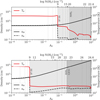 |
Fig. 2 Density and temperature radial profiles for the two models described in Fig. 1. |
| In the text | |
|
Fig. 3 Comparison of the H II, H I, and H2 masses for different architectures. The histograms are built using the MCMC draws for the whole sample. The vertical lines show the minima and maxima of the distributions (dashed lines), the quantiles at 15% and 85% (plain black lines), and the median value (plain red line). |
| In the text | |
|
Fig. 4 Dust and H I masses predicted by single component (left), multi-component (middle), and power law models (right). The red points mark the location of robust means and the ellipses the 1σ uncertainty around the main peak, following the skewed uncertainty ellipses formalism described in Galliano et al. (2021). We report the mean and standard deviation of the Spearman correlation coefficients (ρ) calculated for of the whole sample, at each of the MCMC steps, represented by the shaded kernel density estimate underlying data points. The dashed lines indicate the 1:1 relation and the blue shaded area a deviation of 0.5 dex around the latter relation. |
| In the text | |
|
Fig. 5 Predicted vs. observed CO emission for single-sector model (left column), multi-sector models (middle column), and power law models (right column). The shades, symbols, and legends are described in Fig. 4. |
| In the text | |
|
Fig. 6 Comparison of the M(H2)CO, M(H2)C and M(H2)C+ for different architectures. The histograms are built using the MCMC draws for the whole sample. The vertical lines show the minima and maxima of the distributions (dashed lines), the quantiles at 15% and 85% (plain black lines), and the median value (plain red line). |
| In the text | |
|
Fig. 7 Stacked histograms of the posterior distribution of the total-to-CO-bright H2 masses for the whole DGS sample. The histograms are built using the MCMC draws for the whole sample. The vertical lines show the minima and maxima of the distributions (dashed lines), the quantiles at 15% and 85% (plain black lines), and the median value (plain red line). |
| In the text | |
|
Fig. 8 MH2,total/MH2,CO versus [C II]/CO(l–0) for single component models (left), multi-component models (middle), and power law models (right). The shades and symbols are described in Fig. 4. The dashed gray lines corresponds to the relation from M2O while the dashed red lines show the linear regressions fitted to the combined posterior distribution for the entire sample. We indicate the equations of linear regressions fitted to the 2D-PDF of the whole sample and the associated coefficients of determination R2. |
| In the text | |
|
Fig. 9 Values of the power-law parameters for individual galaxies controlling the density (left), ionization parameter (middle), and cut (right) for each galaxy. The red dots correspond to the means of the lower and upper boundaries of power laws (and pivot point for the broken power law) and the gray lines represent the power laws corresponding to the averages slope values, for each galaxy. |
| In the text | |
|
Fig. 10 Predicted line fluxes for [C II] [C I], and CO emission lines vs. MH2,total for multi-component models with power-law distributions. The predictions for [C II] and CO match well the observed measurements, as shown in Figs. A.3 and 5. The predictions for [C I] are purely model-based, since no measurement is available. The dashed gray lines show the relations from M20 while the dashed red lines show the linear regressions fitted to the combined posterior distribution for the entire sample. The shades, symbols, and legends are described in Fig. 4. We indicate the equations of linear regressions fitted to the 2D-PDF of the whole sample, and the associated coefficients of determination R2. |
| In the text | |
|
Fig. 11 αCII (left), αCI (middle), αCO (right) versus metallicity for power law models. The shades, symbols, and legends are described in Fig. 4. We indicate the equations of linear regressions fitted to the 2D-PDF of the whole sample, and the associated coefficients of determination R2. We also show the Galactic αCO value from B13 and the range of values compatible with it within 30% (gray-shaded area), the αCO vs. metallicity relations from M20, Schruba et al. (2012), Amorín et al. (2016), and Accurso et al. (2017), and the α[CI] vs. metallicity relations from Glover & Clark (2016) and Heintz & Watson (2020). We use a Galactic conversion factor of 3.2 M⊙ pc−2(K km s−1)−1 to correct for the helium mass (factor of 1.36) when comparing to the model prediction of M(H2). |
| In the text | |
|
Fig. 12 Clumpiness parameter (defined by Eq. (11)) vs. predicted [C II]/CO ratio, colorcoded as a function of metallicity. The clumpiness parameter is anti-correlated with the [C II]/CO ratio and has a secondary dependence with metallicity. |
| In the text | |
|
Fig. 13 Relation between the αCO vs. the gas-phase metallicity (left panel) and the clumpiness parameter (right panel), defined by Eq. (11). The Spearman correlation coefficients are calculated for the means of individual galaxies, shown by colored dots. We show the Galactic αCO value from B13 and the range of values compatible with it within 30% (gray-shaded area). |
| In the text | |
|
Fig. 14 ΣSFR vs. Σ(H2+H I). The galaxies associated with a “clumpy CO” distribution are reported in bold in Table A.2 and correspond to Pclumpy ≥ 0.4 (see Eq. (11)), while the others correspond to a “diffuse CO” distribution. Plain lines correspond to the best fits obtained for those two categories, with their 95% confidence intervals shown as shaded-areas, as well as the relations derived for starbursting galaxies and non-starbursting galaxies from Kennicutt & De Los Reyes (2021) and de los Reyes & Kennicutt (2019), respectively. |
| In the text | |
|
Fig. A.1 Cumulative emission lines profiles of some chosen tracers, including the H2 lines for the two models described in Figures 2 and 1. |
| In the text | |
|
Fig. A.2 Predicted versus observed H2 lines for power law models. |
| In the text | |
|
Fig. A.3 Predicted versus observed PDR lines for power law models. |
| In the text | |
Current usage metrics show cumulative count of Article Views (full-text article views including HTML views, PDF and ePub downloads, according to the available data) and Abstracts Views on Vision4Press platform.
Data correspond to usage on the plateform after 2015. The current usage metrics is available 48-96 hours after online publication and is updated daily on week days.
Initial download of the metrics may take a while.