| Issue |
A&A
Volume 673, May 2023
|
|
|---|---|---|
| Article Number | A89 | |
| Number of page(s) | 40 | |
| Section | Extragalactic astronomy | |
| DOI | https://doi.org/10.1051/0004-6361/202245554 | |
| Published online | 10 May 2023 | |
Proximate molecular quasar absorbers
Chemical enrichment and kinematics of the neutral gas⋆
1
French-Chilean Laboratory for Astronomy, IRL 3386, CNRS and U. de Chile, Casilla 36-D, Santiago, Chile
2
Institut d’Astrophysique de Paris, CNRS-SU, UMR 7095, 98bis bd Arago, 75014 Paris, France
e-mail: This email address is being protected from spambots. You need JavaScript enabled to view it.
3
Ioffe Institute, Polyteknicheskaya 26, 194021 Saint-Petersburg, Russia
4
Departamento de Astronomía, Universidad de Chile, Casilla 36-D, Santiago, Chile
5
Centre de Recherche Astrophysique de Lyon, UMR5574, U. Lyon 1, ENS de Lyon, CNRS, 69230 Saint-Genis-Laval, France
6
Observatoire de Paris, LERMA, Collège de France, CNRS, PSL University, Sorbonne University, 75014 Paris, France
7
Department of Astronomy, University of Geneva, Chemin Pegasi 51, 1290 Versoix, Switzerland
8
Inter-University Centre for Astronomy and Astrophysics, Pune University Campus, Ganeshkhind, Pune 411007, India
9
European Southern Observatory, Alonso de Córdova 3107, Vitacura, Casilla, 19001 Santiago, Chile
Received:
25
November
2022
Accepted:
25
February
2023
Abstract
Proximate molecular quasar absorbers (PH2) are an intriguing population of absorption systems that was recently uncovered through strong H2 absorption at a small velocity separation from the background quasars. We performed a multi-wavelength spectroscopic follow-up of 13 such systems with VLT/X-shooter. Here, we present the observations and study the overall chemical enrichment measured from the H I, H2, and metal lines. We combined this with an investigation of the neutral gas kinematics with respect to the quasar host. We find gas-phase metallicities in the range 2% to 40% of the solar value, that is, in the upper-half range of H I-selected proximate damped Lyman-α systems, but similar to what is seen in intervening H2-bearing systems. This is likely driven by similar selection effects that play against the detection of most metal- and molecule-rich systems in absorption. Differences are seen in the abundance of dust (from [Zn/Fe]) and its depletion pattern when compared to intervening systems, however, possibly indicating different dust production or destruction close to the active galactic nucleus. We also note the almost ubiquitous presence of a high-ionisation phase traced by N V in proximate systems. In spite of the hard UV field from the quasars, we found no strong overall deficit of neutral argon, at least when compared to intervening damped Lyman-α systems. The reason likely is that argon is mostly neutral in the H2 phase, which accounts for a large fraction of the total amount of metals. We measured the quasar systemic redshifts through emission lines from both ionised gas and CO(3–2) emission, the latter being detected in all six cases for which we obtained 3 mm data from complementary NOEMA observations. For the first time, we observe a trend between the line-of-sight velocity with respect to systemic redshift and metallicity of the absorbing gas. This suggests that high-metallicity neutral and molecular gas is more likely to be located in outflows, while low-metallicity gas could be more clustered in velocity space around the quasar host, possibly with an infalling component.
Key words: galaxies: active / galaxies: evolution / quasars: general / quasars: absorption lines / quasars: emission lines
Based on observations collected at the European Organisation for Astronomical Research in the Southern Hemisphere under ESO programmes 103.B-0260(A) and 105.203L.001.
© The Authors 2023
 Open Access article, published by EDP Sciences, under the terms of the Creative Commons Attribution License (https://creativecommons.org/licenses/by/4.0), which permits unrestricted use, distribution, and reproduction in any medium, provided the original work is properly cited.
This article is published in open access under the Subscribe to Open model. This email address is being protected from spambots. You need JavaScript enabled to view it. to support open access publication.
1. Introduction
The co-evolution of active galactic nuclei (AGNs) and their host galaxies is regulated by galaxy processes, including secular evolution, the inflow rate of gas (from the intergalactic medium to the interstellar medium and ultimately to the supermassive black hole (SMBH)), and merging history (see Hopkins et al. 2008). The apparent properties of AGNs may further depend on the orientation and the evolutionary stage at which the observations are taken (e.g. Urry & Padovani 1995). This constitutes an entire field of modern astrophysics, motivating large efforts from the community, on both theoretical and observational grounds. Because of the large diversity of observed properties, it is common to select objects based on a few of their many characteristics (e.g. redshift, brightness, colour, radio-loudness, and variability) and study the relations between other marginalised properties. Each of these studies then brings a different and very valuable enlightening angle to the overall picture.
As cold gas constitutes the fuel for both star-formation and the growth of the SMBHs, many works have focused on detecting the dense molecular component of the brightest AGNs (quasars) through CO emission (e.g. Omont et al. 1996; Weiß et al. 2007; Wang et al. 2016) in order to explore the links between star formation, total molecular mass in the host, and growth and activity of the SMBH (e.g. Bischetti et al. 2017).
On the other hand, absorption studies enable detailed investigations of the gas properties along the line of sight to the central engine over a wide range of densities. For example, ionised winds powered by the accretion disc can be observed as broad absorption line systems (BALs) in roughly 15% of quasars, and their velocities range from a few thousand km s−1 up to ∼0.3 c (Hamann et al. 2018). Damped Lyman-α systems (DLAs) are absorption systems whose H I column density (N(H I) > 2 × 1020 cm−2) is high enough for them to be self-shielded from ionising radiation. They are frequently seen along quasar lines of sight (e.g. Prochaska et al. 2005; Noterdaeme et al. 2009). While most DLAs are unrelated to the quasar environment and are only intercepted by chance (called intervening DLAs), some DLAs are found at roughly the same redshift as the background quasar and are hence called proximate DLAs (PDLAs), where ‘proximate’ refers to proximity in velocity space (typically < a few 103 km s−1). Because the redshift path on which PDLAs are identified is much shorter than that available for intervening DLAs, the former are much rarer than the latter. Nonetheless, Prochaska et al. (2008) showed that the incidence of PDLAs (per unit redshift) is higher than expected from the intervening statistics, meaning that they are likely associated with a clustered environment around the quasar.
Ellison et al. (2010) performed the first systematic study of PDLAs at high resolution and concluded that at least a fraction of them exhibit different characteristics relative to the intervening population. They suggested, however, that PDLAs are probably not related to the quasar host, but preferably sample more massive galaxies in the highly clustered region around the quasar. Interestingly, Ly-α emission has been relatively frequently found in the core of several PDLAs (e.g. Møller & Warren 1993; Leibundgut & Robertson 1999; Ellison et al. 2002), when this is more rarely seen among the several 104 known intervening DLAs (but see Fynbo et al. 2010; Noterdaeme et al. 2012; Ranjan et al. 2018 for some example of direct detection, and Rahmani et al. 2010; Noterdaeme et al. 2014; Joshi et al. 2017 for statistical detection through stacking). Finley et al. (2013) and Fathivavsari et al. (2018) further identified a population of PDLAs with Ly-α emission spanning a range of strengths, up to the point at which the H I Ly-α absorption becomes unseen, but the presence of neutral gas is confirmed by strong low-ionisation metal lines. These emissions probably do not arise from star formation, but rather from Ly-α from the AGN that is not fully covered by the absorber. Because Ly-α photons scatter easily and up to large distances around quasars (e.g. Arrigoni Battaia et al. 2019; Borisova et al. 2016), it is not straightforward to conclude about the location, scale, and geometry of the absorbing gas. However, signatures of high excitation of the gas suggest an origin at a rather small distance from the AGN, at least for the most extreme cases.
Noterdaeme et al. (2019, hereafter Paper I) presented a new approach that focused on the presence of strong molecular hydrogen absorption directly detected at the quasar redshift in Sloan Digital Sky Survey (SDSS) spectra, without prior on the presence of H I or metal lines. Not only is H2 sensitive to the physical and chemical conditions in the cold gas, but this approach also differs from studies based on CO molecular emission, for example, in the sense that no prior is made on the overall mass of dense molecular gas in the galaxy host, but rather on the interception of more diffuse cold gas by the quasar line of sight. The strong excess of proximate H2 absorbers with respect to intervening statistics shows that most of these systems must be associated with the quasar environment, although it is not clear whether the absorbers arise from the quasar host or if the excess is due to strong clustering of galaxies around the quasar.
To shed light on this issue, we embarked on a follow-up study with the multi-wavelength medium-resolution spectrograph X-shooter on the Very Large Telescope (VLT). A detailed study of a first system revealed a likely origin in outflowing material intercepted by the line of sight to the central engine (Noterdaeme et al. 2021a, Paper II). Remarkably strong and wide CO(3–2) emission as well as 3 mm continuum emission was detected in the same optically bright (moderately reddened) system through NOEMA observations (Noterdaeme et al. 2021b, Paper III). All this suggests that the nucleus is seen through a channel of lower density, but where some of the molecular content is carried out by outflows when the host still contains large amounts of dust and molecular gas with wide kinematics. This may be indicative of a post-merger system.
In this work, we focus on the overall chemical enrichment and kinematics of the gas of our follow-up sample. In Sect. 2 we present the sample, observations, data reduction, and post-processing. In Sect. 3 we present the column density and dust extinction measurements. In Sect. 4 we present the emission redshifts and absorption line kinematics. We discuss our findings and compare our results with other PDLAs as well as strong intervening H2 systems in Sect. 5. We conclude in Sect. 6.
2. Sample, observations, and data reduction
2.1. Sample and observations
The sample studied here is entirely drawn from Paper I. In the statistical sample of 50 quasars with high-confidence proximate molecular absorbers, 22 have δ < 20°, that is, they can be reached from the southern hemisphere. We obtained VLT/X-shooter data for 13 of them: 11 based on their observability during the allocated periods of this specific programme (P103 and P105, but because of delays related to the observatory shutdown during the Covid-19 pandemic, the observations were actually completed in P109), plus the quasars SDSS J013644.02+044039.1 and SDSS J085859.67+174925.1 for which we used data collected in P94 as part of another programme (Balashev et al. 2019). We note that SDSS J123602.11+001024.5 has already been observed by Balashev et al. (2019). This quasar was then re-observed under better conditions and from various position angles through the availability of the X-shooter atmospheric dispersion corrector. We use the new data here. We finally note that because the quasars in this sample were selected from the statistical sample based upon their observability alone (and not based on any other property), they are likely a fairly good representation of the latter.
X-shooter (Vernet et al. 2011) simultaneously covers the whole optical to near-IR (NIR) wavelength range from 0.3 to 2.5 μm, splitting the incoming light beam into three spectrographs (arms): UVB, ranging from 0.3 to 0.6 μm; VIS, ranging from 0.6 to 1.0 μm; and NIR, ranging from 1.0 to 2.5 μm. All observing blocks (OBs) consisted of 2980 s, 3010 s, and 5 × 600 s exposures for the UVB, VIS, and NIR arms obtained in stare mode. We used 1.0 and 0.9″ wide slits in the UVB and VIS, with slow read-out mode and 1 × 2 pixel binning. The NIR observations were performed with 1.2″ slits for the two quasars observed in P103 (SDSS J001514.82+184212.3 and SDSS J232506.62+153929.3). The remaining observations were performed with a narrower NIR slit (0.9 arcsec) and a K-band blocking filter to avoid stray light in the instrument, effectively cutting out all wavelengths longer than 2.08 μm for all remaining quasars but SDSS J013644.02+044039.1 and SDSS J085859.67+174925.1 (in P94), for which the K-band filter was not yet available. We executed two to five OBs for each quasar at different position angles. Most of the observations were obtained under good seeing, somewhat sharper than the slit widths at the corresponding wavelengths, resulting in higher than nominal spectral resolution. The observing log is given in Table 1. For convenience, we refer to these objects using a short version of their name in the following: SDSS Jhhmmss.ss+ddmmss.s is abbreviated as Jhhmm+ddmm (e.g. J0015+1842 instead of SDSS J001514.82+184212.3).
Quasar sample and log of X-shooter observations
2.2. Data reduction and telluric corrections
All X-shooter spectra were processed using the official esorex pipeline version 3.5.3 (Modigliani et al. 2010) for stare-mode reduction, maintaining the default parameters and including the correction for instrument flexure (recipe xsh_flexcomp). The raw images were pre-processed using the Python package astroscrappy (a reimplementation of the L.A.Cosmic algorithm by van Dokkum 2001) to interpolate over pixels contaminated by cosmic-ray hits using the neighbouring pixels. Each arm of each OB was reduced separately using the standard star observed closest in time in order to flux calibrate the given spectrum. The 1D spectra were then extracted using optimal extraction (Horne 1986).
Next, we used the ESO tool molecfit v.4.2.2a.1 (Smette et al. 2015) to correct each individual 1D VIS and NIR spectrum for the absorption lines produced by the Earth’s atmosphere. In the VIS, the main telluric absorption features are due to O2 and H2O, while the NIR is strongly affected by H2O and CO2 bands. Following the recommendation from the molecfit manual, the correction was made by choosing a few spectral regions with clear but not strongly saturated atmospheric lines for each quasar, typically, 0.68–0.69, 0.71–0.73, 0.76–0.77, 0.81–0.82, and 0.91–0.91 μm in the VIS. In the NIR, we had to adjust the selected spectral regions for each quasar more strongly, depending on the strength of absorption bands and on the location of quasar emission lines. During this process, we also masked deviant pixels (e.g. cosmic remnants) as well as astrophysical lines.
The best-fit model was used to calculate the overall atmospheric transmission and correct the individual VIS and NIR 1D exposures accordingly. The telluric-corrected spectra were then shifted to vacuum-barycentric wavelengths, rebinned to a common wavelength grid, and combined using an inverse-variance weighting. The same vacuum-barycentric correction and combination of 1D spectra was applied to UV data, but without telluric correction.
We note that molecfit also provides the actual spectral resolution, which is a free parameter of the transmission model. As expected from a seeing sharper than the slit widths for most of the observations, the resolving power is typically 25% higher than the nominal values in the documentation (Rnom = 5400 (UV) and 8900 (VIS)). The average spectral resolution obtained from individual VIS spectra is then adopted when fitting the lines. In the UV, the spectral resolution is first estimated by scaling the nominal UV value by the observed-to-nominal VIS resolution ratio. We verified that the values broadly agree with those expected for a slit width that would correspond to the observed seeing. It was then adjusted during the fitting process if necessary. While the exact values have little influence on the metal column densities, we provide the adopted values of the resolutions for the combined spectra along with the best-fit model parameters in Appendix B to facilitate reproducibility.
2.3. NOEMA observations
While the present work focuses on X-shooter data, we also obtained observations with the NOrthern Extended Millimeter Array (NOEMA) and the PolyFIX correlator in the 3 mm band between May 2020 and May 2021 for six out of the 13 objects presented here. The central frequency was chosen in order to cover the expected position of the CO(3–2) emission line, which we detected in all six cases. A description of data handling and analysis of NOEMA observations (including other quasars from the same parent sample that were not observed with X-shooter) will be presented in a future paper, but we already use the redshifts from the detected CO(3–2) emission lines in the discussion (Sect. 5). The Gaussian fits to the CO(3–2) emission lines are presented in Appendix F.
3. Column-density measurements
We analysed the absorption lines through standard, simultaneous, multi-component Voigt-profile fitting using vpfit v.12.3 (Carswell & Webb 2014) to measure the column densities, Doppler parameters, and redshifts. The quasar continuum was evaluated using spline functions, with nodes constrained by the unabsorbed regions and adjusted over strong lines in an iterative way when necessary. In order to best take the blending between the metal, H2, and H I lines into account, the final absorption models were obtained by fitting all lines simultaneously. However, for the sake of presentation, we describe the analysis separately for H I, H2, and metals. The results from the fits are presented in the appendix, and the main derived properties are summarised in Table 2.
Main properties of the proximate absorption systems
3.1. Total HI and H2 column densities
The total H I column densities were mostly constrained from the saturated core of the Ly-α line, which is little sensitive to the exact placement of the continuum on top of the Ly-α emission line of the quasars. Based on the wide wavelength coverage of X-shooter and the relatively high redshifts of quasars (implied by the selection upon H2 in SDSS), all lines from the H I Lyman series are covered by our spectra, allowing us to constrain the H I column density further. While the formal statistical errors from fitting the lines are very small (typically, 0.01–0.02 dex), we note that the continuum placement as well as the choice of fitting regions are necessarily somewhat subjective and might introduce some systematic errors. When we allow for continuum variation using Chebychev polynomials, the uncertainties are smaller than 0.1 dex for similar DLA observations with X-shooter (e.g. Balashev et al. 2019; Ranjan et al. 2020). We hence added a conservative 0.1 dex uncertainty to the error budget.
In all the systems, we confirm strong H2 absorption lines from the Lyman and Werner bands. These are typically detected from rotational level J = 0 to J ∼ 6–7 in our X-shooter spectra. The high column densities imply damped lines in at least the first few rotational levels and hence accurate column densities because lines in this regime do not depend on the Doppler parameter b. We also took into account and fit the detected high rotational levels, assuming the same Doppler parameter and redshift for all H2 lines. However, the derived column densities for the high-J levels are likely to be more sensitive to the assumptions on the Doppler parameters. The b values for H2 lines have been found to depend on the rotational level in several cases (see e.g. Noterdaeme et al. 2007; Balashev et al. 2009). A more detailed study and exploration of systematics is hence needed in order to use these lines to constrain the excitation of the gas and the prevailing physical conditions. This is postponed to a future work, while we focus here on the total column densities, which are dominated by the low rotational levels. The fits to the H2 absorption bands are presented in Appendix A.
In Fig. 1 we compare the total H2 and H I column densities obtained with X-shooter with those derived from the SDSS. In the case of H I the agreement is very good and always better than 0.3 dex. For H2, for which the involved columns are much lower, the agreement remains remarkable (except for the lowest column density system, where the difference is 0.85 dex), in particular because the SDSS values were obtained by visually scaling and matching a template (i.e. assuming single component with fixed Doppler parameter and excitation temperature) to the low-resolution, low S/N SDSS spectra (see Paper I). This agreement is similar to what was found by Balashev et al. (2019) for intervening H2 systems.
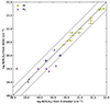 |
Fig. 1. Comparison of H2 (purple diamonds) and H I (green hexagons) column densities obtained using X-shooter and SDSS spectra. The dashed line depicts the one-to-one relation, and the dotted lines show ±0.3 dex around it. |
3.2. Low-ionisation metal species
In this section, we focus on the main low-ionisation metal lines that provide reliable column densities, that is, lines that have multiplets, are not strongly saturated, and do not lie in a region that is strongly affected by telluric lines. For example, we did not attempt to fit the only singly-ionised and very strong carbon line C IIλ1334. We fitted the low-ionisation metal lines assuming a common velocity structure with turbulent broadening (i.e. tied redshifts and Doppler parameters). We first identified the velocity components using the strong Fe II and Si II lines in the visual, which also has higher spectral resolution than UVB, and obtained a first fit, including weaker lines. We then added other metal species and adjusted the fitting regions and the number of components whenever necessary to obtain the final fit.
During this process, we also simultaneously fitted some other intervening systems that posses lines blended with that of the proximate systems, or masked the corresponding blended regions. We also note that Zn IIλ2026 is systematically blended with Mg Iλ2026, which we took into account assuming the same components, although Mg I is not discussed in this work. Whenever possible, we also used Mg Iλ1827 and/or Mg Iλ2852 to further constrain the (small) contribution of Mg I to the 2026 profile. We also took into account partial blending of Zn II with Cr II at 2062 Å. Finally, the analysis of neutral carbon (including fine-structure lines), neutral chlorine, and excited fine-structure lines (from C II, Si II and O I) is post-poned to a future work because we focus here on chemical enrichment, to which their contribution is negligible. We already note the clear detection of Si II* towards J0015+1842, J0019–0137, J0059+1124, J0125–0129, J1259+0309, J1358+1410, J2228-0221. and J2325+1539. The fit to the different metal lines is presented in Appendix B.
We note that the metal column densities obtained at medium spectral resolution should always be considered with some caution because the modelling of the velocity profile mostly implied fewer but broader (b frequently as high as 20 km s−1) components than typically observed in high-resolution spectra, where b < 10 km s−1. Therefore, in spite of our best efforts to model the profiles and use lines with a range of strengths, unresolved line saturation may still affect the column density estimates for some of the species more than the formal uncertainty suggests. Metallicities were derived using weak Zn II lines in all but one case, where the total column densities are less sensitive to the exact velocity structure decomposition.
3.3. Dust
We quantified the amount of dust in the absorbers by measuring the extinction of the quasar, following a template-matching procedure as was used in many works (e.g. Srianand et al. 2008; Ma et al. 2015; Krogager et al. 2016; Zhang et al. 2015). In order to measure the dust reddening using the full wavelength range provided by X-shooter, we combined the spectra from all three arms to obtain a joint spectrum for each quasar. The combination was performed using an inverse-variance weighting in the overlapping regions. During the combination, all three arms were interpolated onto a common wavelength grid using a fixed sampling of 0.2 Å. The joint spectra were finally corrected for Galactic extinction using the map by Schlafly & Finkbeiner (2011).
The individual joint spectra were then fitted using the quasar template by Selsing et al. (2016) assuming a fixed extinction law at the redshift of the quasar. This implicitly assumes that no other intervening absorber causes the reddening. This assumption is reasonable because the proximate systems likely contain most of the dust present along the line of sight, as indicated by H2 and the low probability of intercepting another rare dust-rich absorber by chance. We did not find signs for additional metal-rich intervening absorbers in any of the quasar spectra. Since we observe no evidence of 2175 Å extinction features, we used the extinction law inferred for the Small Magellanic Cloud (Gordon et al. 2003). To avoid biasing the fit, we excluded regions of the spectra around the strong, broad emission lines. We furthermore exclude regions that are affected by strong telluric absorption.
For each target, we derived the dust extinction as the average of the AV values for the individual observations. The statistical uncertainty was determined as the standard deviation of the individual measurements. This uncertainty includes any uncertainty on the flux calibration of the different spectra. Lastly, from previous work, we assigned a systematic uncertainty of 0.07 mag (Noterdaeme et al. 2017) due to any possible intrinsic mismatch of the template and the given target (i.e. accounting for scatter in the intrinsic spectral energy distribution of quasars). The results are summarised in the penultimate column of Table 2, and the fits shown in Appendix C.
4. Absorption line kinematics and systemic redshifts
4.1. Absorption line kinematics
We quantified the kinematics of the neutral absorbing gas using the velocity width as defined by Prochaska & Wolfe (1997): Δv90 = c[λ95 − λ5]/λ50, where λ5, λ50, and λ95 are the wavelengths corresponding to the 5, 50 and 95 percentiles of the apparent optical depth distribution. For each system, we followed the criteria from Ledoux et al. (2006) and selected a few low-ionisation absorption lines that are not too strongly saturated (it would otherwise be impossible to measure the apparent optical depth) nor too weak (in which case, part of the gas would remain untraced). We then checked for consistency between results. The Δv90 for each PDLA is shown in Appendix D and provided in the last column of Table 2.
We note that while the smearing of the lines at medium spectral resolution might result in a small overestimation of Δv90 in principle (Prochaska et al. 2008; Arabsalmani et al. 2015), this is mostly true for low-velocity widths and only becomes an issue when statistics of samples are compared that were taken at different spectral resolutions. Moreover, the spectral resolution and Δv are high enough for the corrections to be negligible here, although, strictly speaking, the lowest values (for J1331+0206 and J1259+0309) might be considered as upper limits.
4.2. Quasar redshifts
A precise measurement of the quasar redshift is then required to study the motion of the absorbing gas with respect to the central engine along the line of sight, and more generally, to investigate dynamical processes in the circum-nuclear region and/or in the host galaxy. Velocity shifts between the different emission lines are seen in quasar spectra, reflecting the diverse kinematics of the emitting regions (e.g. Gaskell 1982; Tytler & Fan 1992; Vanden Berk et al. 2001; Shen et al. 2016). Overall, it was found that high-ionisation lines tend to be strongly blueshifted with respect to the systemic redshift (zsys), while low-ionisation lines provide a better means to measure zsys. The most reliable of these lines are the oxygen lines.
We hence first focused on the [O II] and [O III] lines, which are redshifted in the NIR. Unfortunately, telluric absorption bands frequently affect these lines, and in spite of our best efforts to correct for the atmospheric absorption, it is not always possible to recover the unabsorbed emission line properly. When the lines were reasonably well visible, we modelled the region covering Hβ and [O III] using a simple linear continuum, to which we added Gaussian lines (with more than one component whenever necessary), but we tied the parameters of the two lines of the [O III] doublet together: the same velocity, the same width, and a flux ratio of 3. [O II] was fitted independently. In order to remove spikes, skyline, or cosmic-ray residuals as well as absorption lines, we iteratively fitted the data rejecting deviant pixels (at more than 3σ) at each iteration until convergence (i.e. until no more pixels were rejected). We then visually compared the derived model with the rebinned data obtained from median averaging in bins of typically 25 pixels. Unfortunately, for two [O II] lines, the sky line residuals are close to the peak, and the [O II] redshifts may therefore not be as reliable as expected. This effect is mitigated for [O III], which is generally stronger and has two lines.
In principle, Mg II is the following choice at shorter wavelengths (Shen et al. 2016). We note that owing to our selection on the presence of a proximate absorber, the line is affected by strong Mg II absorption, which we masked during the fitting process. We then also considered the strong C III] and the weaker He II lines at 1908 and 1640 Å rest frame, respectively, which are free from strong absorption. We followed the prescription from Shen et al. (2016) and measured the line redshifts from the peak of the emission, obtained from a model that reproduced the data. Multiple Gaussians provided convenient models through their flexibility and the relatively few free parameters.
The redshifts obtained this way are given in Table 3 using the same rest-frame wavelengths as in Shen et al. (2016). In the case of [O II], [O III], and Mg II, the authors found small systematic shifts (∼8, −45, and −57 km s−1, respectively) compared to the systemic value, which they determined from Ca II absorption. This is less than our measurement uncertainties, therefore we did not attempt any correction here. In the case of the C III] complex (which includes Si III] and Al III), they found a luminosity-independent systematic shift of −229 km s−1, and in the case of He II the systematic shift depends on luminosity. Here we also followed the prescription from Shen et al. (2016) and applied the correction accordingly (see their Eq. (1) and best-fit parameters in their Table 2). We note that these empirical shifts include any possible physical shifts of the emitting regions, plus the fact that several species contribute to the complex. We also provide the corrected redshifts in Table 3 in an attempt to remove the average trends seen in quasars. As the average shifts from Shen et al. (2016) were computed based on low-redshift quasars observed in the SDSS, we finally performed a last test by matching the quasar composite from Selsing et al. (2016) with our data in a region of the visual spectrum covering the range 1620–2450 Å rest-frame, that is, covering the features from He II to [Ne IV]. This range is slightly reduced in a few cases to avoid poor-quality regions, generally at long wavelengths. Absorption lines, bad pixels, and sky-line residuals were masked during the fitting process. The only four free parameters are the scaling value, an additional continuum (power-law+constant), and the redshift.
Measurements of the quasar emission line redshift.
The different measurements (see Appendix E) then allowed us to cross-check the emission redshift and determine the best estimate based on ionised lines (which we call  ), as given in the penultimate column of Table 3. In general, we prioritised the lines following the prescription from Shen et al. (2016), although in some cases, we preferred a second-choice line with high S/N over a line with more uncertain measurement. This was the case for J0136+0440 and J0858+1749, where we preferred the corrected C III] over Mg II, and J1331+0206 where we preferred Mg II over [O II]. At the end, He II and template measurement were not used, but they are provided for comparison and to give more confidence to the measurement. Finally, in the last column of this table, we indicate the redshift of the CO(3–2) emission line derived from fitting the 3 mm NOEMA data with single Gaussian profiles. This is expected to be an even better indicator of the quasar host systemic redshift because it traces the bulk of the molecular gas (Wang et al. 2016). The corresponding fits are shown in Appendix F. Interestingly, the CO-based redshifts appear to be systematically higher by about 250 km s−1 (average based on the six systems for which CO(3–2) measurements are available) with respect to the systemic redshifts based on rest-frame UV/optical transitions. This is discussed in Sect. 5.3.
5. Results and discussions
5.1. Chemical enrichment
In the following, we discuss the chemical properties of our sample based on the measured column densities, and we further compare them with other samples of absorption systems: (1) Proximate H I -selected DLAs observed at high spectral resolution by Ellison et al. (2010); (2) a compilation of intervening DLAs (De Cia et al. 2016) with robust abundance measurements, and (3) a compilation of H2 systems from Balashev et al. (2019) that was confirmed from follow-up observations. This compilation contains H2-bearing systems identified with a number of different selections: in regular DLA systems (Noterdaeme et al. 2008; Balashev et al. 2014, 2017), extreme H I absorbers (Noterdaeme et al. 2015; Ranjan et al. 2020), and C I-selected systems (Ledoux et al. 2015; Noterdaeme et al. 2018). A discussion of the selection function is presented in Balashev et al. (2019), and therefore, we here only consider the sample as a whole, but keep in mind that its distribution in parameter space is a sum of several selections. We removed some systems that have zabs ≈ zQSO and might be considered as proximate from the intervening samples. In order to avoid possible evolutionary effects in our comparison, we also restricted these samples to z > 2. Finally, we removed known H2 systems from the sample by De Cia et al. (2016) to avoid duplicates with Balashev et al. (2019).
We used the standard notation of the gas-phase abundances of the different species X expressed relative to the solar values as [X/H] = log(N(X)/N(Htot)) − log(X/H)⊙, and where we took the solar abundances from Asplund et al. (2021) following the recommendations of Lodders (2003) on whether to take photospheric, meteoritic, or average values (see e.g. Table 1 of Konstantopoulou et al. 2022). We assumed, as is common, that ionisation corrections are negligible for DLAs because of the self-shielding from > 13.6 eV photons, that is, that the considered species are in the main ionisation stage in the neutral gas (e.g. N(Zn II) = N(Zn)). We included H2 in the total hydrogen column density, however, that is, N(H) = N(H I) + 2N(H2). We recall that we considered the gas-phase abundances only when quoting abundances as [X/H]. In other words, we did not attempt any correction for dust depletion. We further investigate this effect by considering volatile and refractory elements in the following sections. A summary of the total abundances of the main species of interest is provided in Table 2.
5.1.1. Overall metallicity from volatile species: Zinc and sulphur
Zinc and sulphur are generally considered as the best reference elements for the intrinsic metallicity (i.e. log Z/Z⊙ ≈ [Zn/H] ≈ [S/H]) because they are volatile and hence little depleted onto dust grains (see e.g. Welty et al. 1999; De Cia et al. 2016, among many other works). We confirm that for all PDLAs where both zinc and sulphur abundances can be measured, the agreement between both values is good, with an average measured sulphur-to-zinc abundance ratio [S/Zn] ≈ 0 and dispersion 0.1 dex (see Fig. 2). We note that, in principle, this does not exclude depletion of both species to similar amounts. However, we would expect any depletion to start differing at higher [Zn/H], which is not apparent. We do not see any trend of [S/Zn] with [Zn/Fe] either. In any case, for a comparison with other measurements in the literature, we continue to assume log Z/Z⊙ ≡ [Zn/H] in the following. For the only system without a Zn measurement (J0136+0440, where the corresponding lines are too heavily blended with atmospheric lines), we hence used sulphur instead. Overall, we found that the metallicities in proximate H2 systems span a range from log Z/Z⊙ ≈ −1.6 to −0.4. This corresponds to the upper half range of H I-selected proximate DLAs, as investigated by Ellison et al. (2010), but is similar to the metallicity of intervening H2-bearing DLA systems (e.g. Petitjean et al. 2006; Balashev et al. 2019).
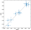 |
Fig. 2. Observed abundance of sulphur against that of zinc in proximate H2 systems. |
5.1.2. Dust depletion from relative abundances
Silicon and iron are refractory elements known to be respectively mildly and strongly depleted onto dust grains, and their gas-phase abundances are typically lower than those of zinc and sulphur. In Fig. 3 we show the abundances ratios [Zn/Fe] and [Zn/Si] as a function of metallicity. These ratios clearly increase with increasing metallicity, as has been observed in a number of works on intervening DLAs (e.g. Ledoux et al. 2003; Noterdaeme et al. 2008; De Cia et al. 2016; Balashev et al. 2019). This can be attributed to the increasing abundance of dust with increasing metallicity.
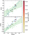 |
Fig. 3. Zinc-to-iron (bottom) and zinc-to-silicon (top) ratio for our sample of proximate H2 systems (circles with error bars). The colour scale provides the value of AV/N(H), which is a proxy of the dust-to-gas ratio. For two systems, the derived AV values are negative (hence unphysical) and the corresponding points are empty. Green triangles represent measurements in intervening DLAs (De Cia et al. 2016), and filled triangles correspond to known H2 intervening systems (Balashev et al. 2019). The solid blue lines show the best linear fit to the value for the proximate H2 systems, taking uncertainties on both axes into account. The green lines and shadowed region show the best linear fit and associated 1σ uncertainty for the overall sample of intervening DLAs. |
Iron appears to be significantly depleted even down to the lowest metallicities, while [Si/Zn] becomes positive only for metallicities higher than one-tenth solar. Interestingly, [Zn/Fe] in proximate H2 systems is clearly higher for a given metallicity than the values seen in regular intervening DLAs, suggesting a higher depletion of iron in proximate systems. This remains true when proximate H2 absorbers are compared only to intervening H2 ones, even if the latter tend to have high depletion among the overall (mostly non-H2 bearing) intervening population at a given metallicity. It is also interesting to see a lower dispersion for proximate systems around the main trend (dotted blue line), likely suggesting a more homogeneous population.
On the other hand, the difference between proximate H2 and intervening systems (regardless of their H2 content) is less clear in the case of [Zn/Si]. Since silicon is an α-element predominantly produced in massive stars, it is possible that a stronger intrinsic depletion (with respect to intervening systems) is compensated for by recent star formation, or that the depletion sequence for Si and Fe differs as well.
In short, the high depletion (from [Zn/Fe]) at a given metallicity suggests a mechanism for build-up and/or destruction of dust grains that is similar in the population of proximate H2 systems, but different from that seen in intervening DLAs. Any correction to account for some depletion of zinc and to recover the intrinsic metallicity could then also be different for proximate systems. We note that if the same depletion sequences as in intervening systems were assumed, the corrected metallicities, following De Cia et al. (2016), would be a factor two higher on average.
The abundance of dust can independently be quantified using the extinction per hydrogen atom, AV/N(H). While the 0.07 mag uncertainty on AV measurements remains quite large compared to their values, there is a clear tendency for higher AV/N(H) at higher [Zn/Fe], [Zn/Si] and metallicities, strengthening a dust-depletion origin for the observed underabundance of iron and silicon. The depletion and value of AV/N(H) strongly correlate with each other with a Pearson coefficient r = 0.9 and a probability of chance coincidence of 0.07%; see Fig. 4. The low dispersion around the approximate linear relation (log AV/N(H) ≈ 1.3[Zn/Fe] − 23.5) indicates that the quasar template matching provides reliable estimates, at least relative to each other. Interestingly, it is also possible to indirectly derive the extinction from the gas-phase abundances, assuming some scaling with respect to the Galactic values. We represent this in Fig. 4 as well, based on calculations following De Cia et al. (2016). These values appear to agree relatively well with the reddening-based measurements, but the former are higher by 0.25 mag on average than the latter. This may be another indication for a different type of dust close to the quasar. However, a comparison of extinction derived from gas-phase abundances with that directly obtained from the spectral slope should be performed first in intervening systems to validate the prescription by De Cia et al. (2016) at this precision level.
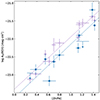 |
Fig. 4. Dust-to-gas ratio measured from the continuum spectrum (filled circles) and derived from the metal column densities (open diamonds, following De Cia et al. 2016) as a function of depletion factor. The blue (purple) dotted line corresponds to a linear fit to ([Zn/Fe], log AV/N(H)) data points, where Av is based on continuum fitting (metal column density). |
5.1.3. Sulphur-to-silicon ratio in proximate absorption systems
The [S/Si] ratio is also an interesting quantity because both species are α elements and their intrinsic abundances are expected to follow each other. According to Ellison et al. (2010), based on modelling by Rix et al. (2007), the observed negative [S/Si] values at low H I column densities in their sample of PDLAs is due to ionisation by a hard spectrum. We compare this ratio in our sample of proximate systems with those from Ellison et al. (2010) as a function of the H I column density in Fig. 5. In contrast to what these authors observed in PDLAs, we observe no drop in [S/Si] below log N(H I) = 20.75 in our strong H2-bearing PDLAs. While we did not probe H I columns as small as these authors, it is interesting to note that both PDLAs and PH2 have close to solar ratios at high column densities log N(H I) > 21. In contrast with the PDLAs from Ellison et al. (2010), we see a tendency for increasing [S/Si] with decreasing H I column, which is opposite to what is expected if these ionisation corrections are at play, but rather reflects an increasing depletion with decreasing H I. This can be due to a bias against systems with high column densities of dust that would either be excluded from the parent quasar sample (Ledoux et al. 2009; Augustin et al. 2018) or result in a low S/N of the corresponding spectra. It can also be due to a higher abundance of metals or dust required for the presence of H2 at low H I column densities (e.g. Bialy et al. 2017), thereby increasing the dust shielding, H2 formation rate, and gas cooling through atomic lines. In the low N(H I) regime, we would qualify the observed [S/Si] in (non-H2) PDLAs as highly dispersed and possibly interpret this as a wide range of ionisation.
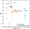 |
Fig. 5. Sulphur-to-silicon abundance ratio vs H I column density. The horizontal dashed line marks the solar ratio, and the vertical line shows the N(H I) limit below which Ellison et al. (2010) observed lower-than-solar abundances in PDLAs (see text). While not in our sample of proximate H2, one PDLA from Ellison et al. (2010), namely J2340-00, also has strong H2 and is marked with a blue circle. |
To investigate the effect of differential dust depletion further, we plot [S/Si] as a function of [Zn/Fe] in Fig. 6. Here, the correlation between the two abundance ratio is apparent in the case of proximate H2 systems (Pearson correlation coefficient of 0.76 with a 0.4% probability to be due to chance coincidence). This favours depletion of silicon as a more likely origin for the high [S/Si] values. Fitting a linear relation to the proximate H2 data that takes uncertainties on both axes into account, we obtain [S/Si]≈0.39(±0.08)×[Zn/Fe]−0.21(±0.09). A correlation between the two abundances ratio has also been observed in intervening DLAs (Pearson correlation r = 0.7), for which we show the best-fit linear relation obtained by De Cia et al. (2016) together with the associated intrinsic dispersion1. However, proximate systems differ from intervening DLAs in the sense that they have [S/Si] ≈ 0 for a wider range of [Zn/Fe] values. This is observed for PDLAs regardless of whether they contain H2 when the intercept for intervening DLAs is almost zero.
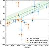 |
Fig. 6. Sulphur-to-silicon vs zinc-to-iron abundance ratios in proximate H2 and DLA systems. The green line and shaded area represent the best fit for intervening DLAs by De Cia et al. (2016) and the 1σ scatter around this relation. The dashed blue line is a linear fit to the proximate H2 data. Dashed vertical and horizontal lines mark solar values. Symbols and colours for data points are as in Fig. 5. |
In summary, the PH2 systems with high [S/Si] values appear to behave like intervening DLAs. The five systems with highest values also have low H I column densities, which is naturally explained if high-H I high-depletion systems are missing due to dust bias. At low [Zn/Fe] (and high N(H I)), the [S/Si] values tend to differ between intervening and proximate systems, the latter having typically lower observed [S/Si] from S II and Si II closer to solar. We conclude that the main driver of the [S/Si] ratio is depletion onto dust, with a possible different depletion sequence than that seen for intervening DLAs, again suggesting a different dust type proximate to the quasar. However, ionisation effects might still be at play, meaning that part of these low-ionisation metals might arise from ionised gas. Larger samples of proximate DLAs (with and without H2) are necessary to investigate this further.
5.1.4. Argon as a probe of a hard UV ionising field
Argon can provide an additional diagnostic on the ionising field. Owing to its high first-ionisation energy (15.76 eV), argon is expected to be mostly neutral in DLAs, which are self-shielded against H I-ionising photons. While argon is predominantly ionised by cosmic rays in the local ISM, high-energy photons significantly above 13.6 eV can still penetrate the cloud and ionise argon, which further has a low recombination to ionisation rate in diffuse atomic medium (see e.g. Sofia & Jenkins 1998). Zafar et al. (2014a) found a deficiency of argon by about 0.4 dex (with standard deviation about 0.2 dex) with respect to other α-elements in intervening DLAs, with a weak dependence on H I column density. They concluded that because argon is extremely volatile (Lodders 2003), the argon deficit is likely dominated by ionisation from the quasar metagalactic radiation, with local modulation by H I column inside the absorbing galaxies.
We constrained the Ar I column densities in our sample of proximate H2 absorbers using the two available absorption lines (at 1048 and 1066 Å). Because these fall into the Lyman-α forest and can easily be blended with H2/HD lines, we used a slightly different procedure: We fitted the Ar I lines by fixing the redshifts and Doppler parameters to that previously obtained for other metal metal lines and fitting for the column densities. We included the H2 absorption profile constrained by the independent fit (see Sect. 3.1) and avoided blends with the Ly-α forest as best as possible. In a few cases, however, we were unable to obtain a meaningful constraint. The fit to the argon lines is shown in Fig. B.10.
The derived [Ar/S] (obtained from Ar I and S II) values are shown as a function of the total H I column densities and overall metallicities in Fig. 7. First, we do not see any dependence of [Ar/S] on N(H I), in agreement with the expected lack of shielding by neutral hydrogen. We do not see any dependence on overall metallicity either, in contrast to the possible negative (but not easily explained) trend seen by Zafar et al. (2014a). The lack of a dependence on overall metallicity is in line with the expected non-depletion of argon onto dust. Second, [Ar/S] is found to be very similar (−0.35 dex on average) to that seen in intervening DLAs, which could be surprising given the proximity of the quasar. However, our measurements can still be affected by Ly-α interlopers so that the Ar I columns should in principle be considered as upper limits in a conservative approach2, but more importantly, the metal column density is generally dominated by the H2-bearing component, where we observe a lower deficit of argon (−0.2 dex) with respect to components without detectable H2 (−0.7 dex). In Fig. B.10, we also show the expected Ar I profiles obtained assuming a solar [Ar/S] ratio. This over-predicts the absorption in most cases, but this over-prediction also appears to be less severe at the velocity of H2 components.
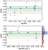 |
Fig. 7. Observed [Ar/S] ratio (based on Ar I and S II) as a function of overall metallicity (top) and H I column density (bottom) in our sample of proximate systems. Blue circles correspond to the overall value in each system, and purple diamonds and red crosses show the H2 and non-H2 components, respectively. The dashed lines correspond to the corresponding mean values. The distribution is shown in the side panel. The green line corresponds to the mean [Ar/S] value (corrected to the same solar reference) and dispersion for intervening DLAs (Zafar et al. 2014b). Even though we tried to take blends into account, all points should be considered as upper limits in principle. |
The relatively low deficit of argon in H2 components is most likely a result from an efficient conversion of Ar+ into neutral argon through chemical reactions with H2 (Ar+ + H2 → ArH+ + H followed by  (see Duley 1980; Schilke et al. 2014; Neufeld & Wolfire 2016). The situation could be similar to that with neutral chlorine (Balashev et al. 2015) and all argon being in neutral form in the presence of H2.
In the regions where hydrogen is predominantly atomic, the ionisation fraction of argon should in turn be very dependent on the ionising field. At higher IUV, the photo-ionisation rate indeed increases while the H2 abundance decreases, impeding the molecular-ion recombination route. Hence the ionisation fraction of argon should rise at least proportionally to IUV. Therefore, the systematically lower abundance in non-H2-bearing components confirms that the medium is likely exposed to a significantly enhanced (and hard) radiation field and/or cosmic-ray ionisation. While quantitative statements would require a full modelling of the observed column densities and a better-assessed association between H2 and metal components (i.e. at high spectral resolution), which is beyond the scope of this paper, we can estimate that the −0.2 dex deficit of argon means that about half of the metal column seen at the velocity of H2 components could come from their (H2-free) H I-envelope where argon would be mostly in ionised form.
5.2. H2 in proximate versus intervening systems
We compare proximate and intervening systems according to their H2 and total hydrogen column densities in Fig. 8. The absence of proximate systems at low H2 columns is naturally due to our selection based on the presence of strong H2 Lyman-Werner bands (Paper I), and all our systems have log N(H2) > 18.5. Proximate H2 were in turn selected independently of N(H I), but as this figure shows, they are limited to log N(H) > 20.5 when intervening systems can have lower N(H) even at similar H2 column densities (see the distributions at the top of this figure). However, this is driven by a few very metal-rich intervening absorbers (as can be seen from the colour coding), two of them following a C I-based selection, skewed towards very high metallicities. Metallicities tend to increase with decreasing N(H) and increasing N(H2). This might naturally be explained by the 1/Z dependence of the critical column density for H2 to form (e.g. Krumholz et al. 2008), but also to a bias against high-metallicity systems at high-N(H I) due to stronger dust extinction.
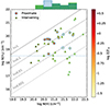 |
Fig. 8. Column density of molecular hydrogen vs total neutral hydrogen column density N(H I) = N(H I) + 2N(H2) for our sample of proximate H2 absorbers and z > 2 intervening strong H2-bearing DLAs from Balashev et al. (2019). For a fair comparison, we removed systems that may potentially be proximate, and kept only systems with a conservative cut of c (zabs − zQSO)/(1 + zQSO) < − 10 000 km s−1. Our selection of proximate H2 systems based on strong H2 lines directly seen in the low-resolution SDSS spectra naturally skews our sample to high H2 columns. The horizontal blue line shows the approximate and empirical lower limit of at log N(H2) > 18.5 for the present sample. The top histograms show the N(H) distributions for the proximate (blue) and intervening (green) systems with N(H2) > 18.5. Finally, the different lines correspond to different averaged molecular fractions fH2 ≡ 2N(H2)/2N(H2) + N(H I)). |
This is better visible in Fig. 9, in which the location H2 systems is shown in the N(H)-Z plane. The different lines show the ratio of UV intensity to number density as a function of the H I column density in the envelope of a single H2 cloud illuminated on one side, following Eq. (2) of Paper I, based on theoretical calculations by Bialy et al. (2017) and where we used Z/Z⊙ as a proxy for  , the grain Lyman-Werner photon absorption cross section per hydrogen nucleon normalised to the fiducial Galactic value. We note that these calculations do not provide the column density of H2, which just continues to build up as more gas would be added to a given cloud. In practice, the total column is dominated by H I, so that the plot against N(H I) only is almost identical. Three-quarter (9 out of 12) of the proximate H2 systems are located between the IUV/n = 10−2 and 10−1 cm3 lines, suggesting similar physical conditions. We caution, however, that the measured H I column corresponds to that integrated over the profiles, while the calculations provide the H I column that participates in the shielding of H2 clouds. Any atomic gas, with some amount of dust, that is located upstream along the line of sight will still participate in shielding H2 from the quasar field.
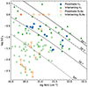 |
Fig. 9. Metallicity vs total hydrogen column density. The different lines correspond to the hydrogen column density of a single H2 cloud illuminated by a UV field for different UV to density ratios IUV/n as indicated above each line, with IUV in units of the Draine field and n in cm−3. Filled symbols correspond to H2-bearing systems. Proximate H2 systems are from this work, proximate DLAs from Ellison et al. (2010), and intervening systems from Noterdaeme et al. (2008) and Balashev et al. (2019). |
Determining the physical conditions from population levels is thus necessary to constrain the distances of the cloud from the AGNs. Owing to the different selections, intervening H2 systems in turn tend to have a wider spread of values. We also note that the lines of constant IUV/n closely follow the constant metal column density (for volatile species), and hence almost constant extinction (e.g. Vladilo et al. 2006). In other words, the conditions that facilitate the presence of H2 are also those that can extinguish the background sources to the point that may be excluded from the optically selected samples. However, since most of the intervening systems were also detected towards quasars from the SDSS, it is likely that more reddened quasars with more metal-rich proximate H2 absorbers are already present in the SDSS database, in particular because these systems could afford lower densities to survive, but the S/N achieved in the blue prevented their detection directly from H2 lines.
We also show in Fig. 9 the location of proximate and intervening DLAs without strong H2 as open symbols. In the case of intervening non-H2 systems, we used the sample from Noterdaeme et al. (2008), for which H2 has been systematically assessed. The fact that no H2 is detected, even at high metallicity and H I column density, means that the corresponding system does not fulfil the requirements for IUV/n. For example, for a UV field about one-tenth of the Draine field, these systems would have low number densities n < 1 cm−3 (which is typical for the warm neutral phase), which is too low to build up molecular hydrogen. Alternatively, their total H I column density is spread over many different clouds. We finally note that the above implicitly assumes static equilibrium, which may not necessarily be the case, in particular if H2 is found in outflowing gas. For n = 100 cm−3 , the characteristic timescale for H2 formation indeed is ∼107 yr, which is then comparable to the dynamical timescales.
5.3. Kinematics
The velocity extent of low-ionisation metal lines Δv90 is considered as a good way to quantify the kinematics of the neutral gas (because this information is not available from the H I lines). In the case of intervening DLAs, Ledoux et al. (2006) first observed a correlation between this velocity width and the gas metallicity, suggesting that this reflects an underlying relation between mass and metallicity because the motion of low-ionisation lines is expected to be governed by gravity. This has been discussed in a number of subsequent works (Møller et al. 2013; Neeleman et al. 2013; Christensen et al. 2019), with attempts to connect this to the mass-metallicity relation seen in emission (e.g. Møller & Christensen 2020). While the assumption that Δv90 primarily depends on the galaxy mass seems to be consolidated at least in a statistical sense, there is evidence that outflows, tidal streams, and the environment in general can affect the velocity spread in a more complex way (e.g. Zou et al. 2018; Nielsen & Kacprzak 2022). Because of the presence of the quasar, the situation might be expected to be even more complex in proximate systems. For example, the case of J0015+1842 is strongly suggestive of outflowing material (Paper II). Surprisingly enough, the distribution of Δv90 in proximate H2 systems follows the trend, and dispersion seen in intervening DLAs, although it is limited to high values, as expected from the presence of H2 (Noterdaeme et al. 2008). Overall, the velocity spread of the neutral gas in proximate H2 systems suggests an origin in massive galaxies, but without a clear indication of perturbed kinematics, or at least, not more perturbed than similar high-metallicity systems in the intervening population (see Fig. 10).
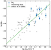 |
Fig. 10. Metallicity vs velocity extent of the low-ionisation metal lines for our sample of proximate H2 systems and a sample of intervening DLAs (mostly from Ledoux et al. 2006 with some additions by Noterdaeme et al. 2008). The green line shows the best-fit relation for high-z intervening DLAs by Ledoux et al. (2006). |
In order to investigate now the kinematics of the gas with respect to the quasar, we represent in Fig. 11 the kinematics of the neutral gas as a function of its metallicity. There is an apparent trend for high-metallicity systems to be around the quasar systemic redshift as obtained from the ionised lines, while low-metallicity systems tend to be redshifted. The Pearson correlation coefficient between v50 = c(zQSO − z50)/zQSO (i.e. the velocity of the centroid of the absorption profile), and the gas metallicity is r = −0.50 with a p-value 0.08. In other words, the probability is only about 8% that this anti-correlation is due to chance alone. One system, towards J0858+1749, is significantly more blueshifted than the rest of the sample. This does not drive the correlation, however, as removing it from the correlation test only changes the Pearson values to r = −0.49, p = 0.10. The ∼2000 km s−1 blueshift of this system makes it intermediate between what could be considered as clearly intervening or proximate. For example, at this velocity, the incidence of strong H2 absorbers already reaches that of intervening absorbers (see Fig. 3, Noterdaeme et al. 2019). The derived UV flux in this system (Balashev et al. 2019) suggests that this system is located farther from the quasar, at a distance of at least several hundred kiloparsec. To account for the statistical uncertainties on metallicity and on the quasar systemic redshift, we calculated the Pearson (r,p) values for 10 000 random samples, for which the metallicity of each system was taken using a normal distribution around the best value with the corresponding uncertainties. Similarly, the velocity was chosen using a normal distribution around the measured value, with σ set to the intrinsic velocity dispersion of zQSO provided by Shen et al. (2016; i.e. 46, 56, 205, and 233 km s−1 for zQSO based on [O II], [O III], Mg II and C III], respectively). From this exercise, we find an approximate normal distribution of r values, giving r = −0.47 ± 0.09 (r = −0.44 ± 0.11 ignoring J0858+1749). The p-values have a median of 0.11 (0.14), but with some tail towards higher values. In short, this means that the trend remains even when statistical uncertainties on metallicity and emission redshift measurements are taken into account.
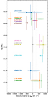 |
Fig. 11. Summary of absorbing gas metallicity and kinematics. The differently coloured segments represent the Δv90 regions, and dots indicate the location of H2 components. The zero of the velocity scale is set to the best estimate of the systemic redshift zsys from ionised lines (Sect. 4.2). Positive velocities mean here |


In principle, the projected line-of-sight velocity towards the quasar for low-metallicity systems could be interpreted as neutral gas infalling onto the quasar host galaxy. However, it is unlikely that gas would feed the quasar directly, and we may instead expect any feeding gas to orbit the quasar host galaxy without a significant line-of-sight velocity component. It is possible, however, that gas orbits the galaxy on non-circular orbits after a galaxy companion interaction, where the outer neutral gas returns as a fountain after having been dragged out in a tidal tail.
Alternatively, the systemic redshift might be underestimated if the blueshifts of the emission lines are higher than observed by Shen et al. (2016). In their work, the authors used Ca II absorption as a reference to compute the (non)-shifts of [O II] and [O III] and then the shift from other lines (Mg II, C III], etc.) are computed with respect to the latter. The use of SDSS data (covering wavelengths shorter than 10 400 Å) implies that the computed shifts correspond to low- to intermediate-redshift quasars (which therefore are likely not particularly luminuous). At high redshifts (z ∼ 5 − 7), Schindler et al. (2020) and Eilers et al. (2021) found higher Mg II blueshifts in luminuous quasars, using precise systemic redshifts from [C II]158μm and/or CO emission line measurements from ALMA and NOEMA as reference. These lines arise from star formation and molecular gas, respectively, and hence should better represent the systemic redshift of the quasar host, which is also very likely to dominate other lower-mass galaxies in the quasar group. The sample presented here has redshifts z ∼ 3, so that we may naively expect line shifts in between those obtained by Shen et al. (2016) and those obtained by Schindler et al. (2020) or Eilers et al. (2021). For half of our sample, we have CO(3–2) redshifts from our NOEMA observations, which we represent as ellipses in Fig. 11. The CO redshifts are about 250 km s−1 higher om average than those obtained from the (corrected) ionised emission lines. If zCO represents better estimates of the host galaxy redshift, then the absorbing gas now appears to have no particular line-of-sight velocity at low metallicities, while the outward velocities at high metallicities is reinforced. This maintains the anti-correlation to r ≈ −0.6, p ≈ 0.2 (now computed on six quasars). In this case, high-metallicity gas (above ∼25% solar) is more likely to represent gas enriched by intense star formation activity that is expelled through associated winds, as is clearly seen in the case of J0015+1842 (Paper II), which has the highest metallicity in our sample. This would be consistent with chemically enriched outflowing gas coming from nuclear regions, in contrast to outer gas, due to the radial Z-gradient.
Determining the distances between the absorbing gas and the active nucleus by modelling the excitation of molecular and atomic species should help understanding the origin of the gas with different metallicities further. This study using the present sample is devoted to a future paper.
5.4. AGN proximity from the presence of N V
While we focused on the neutral phase (and low ionization metal species) in this paper, we briefly discuss here the presence of N V absorption at the quasar redshift. Photo-ionisation of nitrogen to this stage requires an energy of 77.5 eV, meaning a hard ionisation spectrum because stellar light falls rapidly after 54 eV, when He II ionisation occurs. This makes N V one of the best diagnostics for the physical proximity of the AGN and distinguishes between intervening and associated system (e.g. Perrotta et al. 2016). Fox et al. (2009) found that N V is detected in only 13% of the intervening DLAs, but they also found a surprisingly similar fraction in PDLAs out to 5000 km s−1, suggesting that proximity in velocity does not necessarily mean physical proximity. 5000 km s−1 in the Hubble flow corresponds to about 16 Mpc proper distance at z ∼ 3. Ellison et al. (2010) found a tentative excess of N V detection rate (2 out of 7) at similar velocities in their PDLA sample, but we note that this fraction would increase if they had limited the statistics to smaller velocity separations from the quasar. Finally, using composite spectra of about one thousand C IV absorbers and interpreting their results with the help of ionisation modelling, Perrotta et al. (2018) confirmed that N V is only present in proximate systems and concluded that it is a good tool for identifying gas that is physically related to the quasar host. N V absorption is clearly seen at the quasar redshift for 9 out of our 13 proximate H2 absorbers (see Fig. A.1). The non-detection of N V in the two systems with the lowest metallicity in our sample may just be due to column density effect rather than lower ionisation. Overall, the very high incidence of N V in our sample supports an origin in the close environment of the quasars. Ionisation modelling, together with comparative kinematic (N V is typically present over wider velocity ranges than low-ionisation species), should help us to understand the ionised component of H2-selected proximate systems.
6. Conclusion
The chemical enrichment and velocity dispersion of the neutral gas in strong proximate H2 systems appears not to be significantly different from what is seen in intervening systems. While the metallicities in proximate H2 systems are higher than the general population of intervening DLAs and are in the upper half when compared to the sample of proximate DLAs from Ellison et al. (2010), they are consistent with intervening systems that also have high H2 content (see Balashev et al. 2019). The relative abundances of sulphur, silicon, iron, and zinc follow the expected trends due to increasing depletion of refractory elements with increasing metallicity (e.g. De Cia et al. 2016), indicating an increased abundance of dust with increasing chemical enrichment. This is also confirmed independently by the increasing quasar extinction per hydrogen atom with depletion and metallicity. We note, however, the higher depletion of iron in proximate systems compared to intervening sytems at given metallicity, suggesting different dust production and/or destruction close to the AGN. The ubiquitous presence of N V absorption indeed indicates a strong and hard UV field, which also explains the deficit of neutral argon in non-H2-bearing components. Argon in turn remains predominantly in neutral form in the presence of H2, aided by ion-molecule reactions.
The lack of proximate and intervening systems with both high-metallicity (or depletion) and hydrogen column density is likely due to a selection effect against highly reddened systems, which would be more severe than just exclusion from optically selected quasar samples. Systems like this may already be present in the SDSS quasar database, but not selected through H2 absorption because of their low S/N in the blue. These systems would also be interesting to recover because they should be able to survive with relaxed densities for a given intensity of UV field (i.e. distance to the central engine). Upcoming surveys should also provide less biased samples of quasars and absorbers. For example, 4MOST (de Jong et al. 2019) will collect optical spectra of quasars selected on astrometry (The 4MOST–Gaia Purely Astrometric Quasar Sample, 4G-PAQS; PI: Krogager), infrared, or X-ray properties (Merloni et al. 2019). The higher spectral resolution and larger collecting area should push deeper into the dust-obscured population of absorbers. Similarly, the MeerKAT Absorption Line Survey (MALS; Gupta et al. 2016) also uncovers quasars in a dust-unbiased manner, owing to the radio+IR selection of the targets (see Krogager et al. 2018; Gupta et al. 2022a). A complementary view of proximate cold gas absorbers can then be done through associated 21 cm absorption. Furthermore, 21 cm absorption provides different (and multiple) lines of sight because radio-continuum emission regions are distinct from the region that produces the optical continuum (Gupta et al. 2022b).
The significant excess of proximate H2 systems with respect to the expected incidence from the intervening statistics showed that most of the former are very likely to be associated with the quasar environment (quasar host or galaxies in the quasar group). On the other hand, the similar column densities of neutral and molecular hydrogen at similar metallicities when compared to intervening H2-bearing DLAs means that proximate H2 should have similar UV-to-density ratios. This means that proximate H2 systems should have a significantly higher density than their intervening analogues if they are located within the dominating influence of the quasar UV field (i.e. within the host galaxy, or possibly several hundred kiloparsec away). The higher densities if located close to the quasars would explain the higher fraction of systems with excited atomic fine-structure lines. Si II* is indeed clearly detected in 8 out of the 13 systems presented here. Determining the physical conditions is necessary in that respect as well.
While our parent sample was selected by having zabs ≈ zQSO, the systems might have been found within a wide velocity range around the quasar owing to the large uncertainties on the quasar emission redshifts in SDSS spectra, together with the low S/N and resolution, allowing H2 detection over a relatively wide range. It is then almost surprising to find that all systems but one were found to have velocities significantly lower than 1000 km s−1 from the quasar, after securing precise absorption and emission redshifts. In the absence of peculiar motions (i.e. pure Hubble flow), this would correspond to at most a few million parsec. If peculiar motions contribute significantly to the observed velocities, then this becomes an upper limit to the actual distance. Velocities of zabs > zQSO systems indicate the dispersion due to peculiar velocities because this clearly cannot be due to the Hubble flow. The kinematics are then all consistent with no Hubble-flow component at all (except for J0858+1749), suggesting that most systems are indeed associated with the quasar host or its group environment.
We observe a trend for different line-of-sight velocities of the absorbing gas with respect to the quasar as a function of metallicity. When we assume systemic redshifts from ionised lines, this would suggest that low-metallicity gas tends to move towards the quasar. However, it is more likely that the low-metallicity gas is more clustered (in velocity space) around the quasar, as corroborated by the use of CO-based redshifts, and that the high-metallicity gas more likely arises from outflowing winds. While this remains speculative for now, if it is confirmed in a large sample of systems, including non-H2 systems, the relation between the motion of neutral gas with respect to the quasar host galaxy and/or the central engine and the chemical enrichment of this gas would open a new window for understanding quasar evolution.
Selection effects appear to be complex in proximate systems, however. For example, the classical selection of PDLAs based on saturated cores biases the samples against systems with leaking Lyman-α emission, which is observed in about half of our proximate H2 systems. If, as expected, the amount of gas and its distribution around the quasar affects the ability of Lyman-α photons to scatter at large distances, this bias will also affect any conclusion on the nature of proximate systems.
We conclude that proximate systems have a strong potential for investigating many processes that drive the evolution of quasars. Determining the physical conditions and distances of gas clouds from the central engine is the next natural step in this matter.
The differences in adopted solar values between this work and De Cia et al. (2016) only affect the [Zn/Fe] ratio by 0.005 dex and hence can safely be ignored here.
This should be less of an issue at high spectral resolution, as in the work by Zafar et al. (2014a), which was based on UVES data.
Acknowledgments
We thank the anonymous referee for useful comments and suggestions. The research leading to these results has received support from the French Agence Nationale de la Recherche under ANR grant 17-CE31-0011-01/project “HIH2”. R.C. gratefully acknowledges support from the French-Chilean Laboratory for Astronomy (IRL 3386). S.L. acknowledges support by FONDECYT grant 1191232.
References
- Arabsalmani, M., Møller, P., Fynbo, J. P. U., et al. 2015, MNRAS, 446, 990 [NASA ADS] [CrossRef] [Google Scholar]
- Arrigoni Battaia, F., Hennawi, J. F., Prochaska, J. X., et al. 2019, MNRAS, 482, 3162 [NASA ADS] [CrossRef] [Google Scholar]
- Asplund, M., Amarsi, A. M., & Grevesse, N. 2021, A&A, 653, A141 [NASA ADS] [CrossRef] [EDP Sciences] [Google Scholar]
- Augustin, R., Péroux, C., Møller, P., et al. 2018, MNRAS, 478, 3120 [CrossRef] [Google Scholar]
- Balashev, S. A., Varshalovich, D. A., & Ivanchik, A. V. 2009, Astron. Lett., 35, 150 [NASA ADS] [CrossRef] [Google Scholar]
- Balashev, S. A., Klimenko, V. V., Ivanchik, A. V., et al. 2014, MNRAS, 440, 225 [NASA ADS] [CrossRef] [Google Scholar]
- Balashev, S. A., Noterdaeme, P., Klimenko, V. V., et al. 2015, A&A, 575, L8 [NASA ADS] [CrossRef] [EDP Sciences] [Google Scholar]
- Balashev, S. A., Noterdaeme, P., Rahmani, H., et al. 2017, MNRAS, 470, 2890 [CrossRef] [Google Scholar]
- Balashev, S. A., Klimenko, V. V., Noterdaeme, P., et al. 2019, MNRAS, 490, 2668 [NASA ADS] [CrossRef] [Google Scholar]
- Bialy, S., Bihr, S., Beuther, H., Henning, T., & Sternberg, A. 2017, ApJ, 835, 126 [NASA ADS] [CrossRef] [Google Scholar]
- Bischetti, M., Piconcelli, E., Vietri, G., et al. 2017, A&A, 598, A122 [NASA ADS] [CrossRef] [EDP Sciences] [Google Scholar]
- Bolatto, A. D., Wolfire, M., & Leroy, A. K. 2013, ARA&A, 51, 207 [CrossRef] [Google Scholar]
- Borisova, E., Cantalupo, S., Lilly, S. J., et al. 2016, ApJ, 831, 39 [Google Scholar]
- Carilli, C. L., & Walter, F. 2013, ARA&A, 51, 105 [NASA ADS] [CrossRef] [Google Scholar]
- Carswell, R. F., & Webb, J. K. 2014, Astrophysics Source Code Library [record ascl:1408.015] [Google Scholar]
- Christensen, L., Møller, P., Rhodin, N. H. P., Heintz, K. E., & Fynbo, J. P. U. 2019, MNRAS, 489, 2270 [NASA ADS] [CrossRef] [Google Scholar]
- De Cia, A., Ledoux, C., Mattsson, L., et al. 2016, A&A, 596, A97 [NASA ADS] [CrossRef] [EDP Sciences] [Google Scholar]
- de Jong, R. S., Agertz, O., Berbel, A. A., et al. 2019, The Messenger, 175, 3 [NASA ADS] [Google Scholar]
- Duley, W. W. 1980, MNRAS, 190, 683 [CrossRef] [Google Scholar]
- Eilers, A.-C., Hennawi, J. F., Davies, F. B., & Simcoe, R. A. 2021, ApJ, 917, 38 [NASA ADS] [CrossRef] [Google Scholar]
- Ellison, S. L., Yan, L., Hook, I. M., et al. 2002, A&A, 383, 91 [NASA ADS] [CrossRef] [EDP Sciences] [Google Scholar]
- Ellison, S. L., Prochaska, J. X., Hennawi, J., et al. 2010, MNRAS, 406, 1435 [NASA ADS] [Google Scholar]
- Fathivavsari, H., Petitjean, P., Jamialahmadi, N., et al. 2018, MNRAS, 477, 5625 [NASA ADS] [CrossRef] [Google Scholar]
- Finley, H., Petitjean, P., Pâris, I., et al. 2013, A&A, 558, A111 [NASA ADS] [CrossRef] [EDP Sciences] [Google Scholar]
- Fox, A. J., Prochaska, J. X., Ledoux, C., et al. 2009, A&A, 503, 731 [NASA ADS] [CrossRef] [EDP Sciences] [Google Scholar]
- Fynbo, J. P. U., Laursen, P., Ledoux, C., et al. 2010, MNRAS, 408, 2128 [NASA ADS] [CrossRef] [Google Scholar]
- Gaskell, C. M. 1982, ApJ, 263, 79 [NASA ADS] [CrossRef] [Google Scholar]
- Gordon, K. D., Clayton, G. C., Misselt, K. A., Landolt, A. U., & Wolff, M. J. 2003, ApJ, 594, 279 [NASA ADS] [CrossRef] [Google Scholar]
- Gupta, N., Srianand, R., Baan, W., et al. 2016, in MeerKAT Science: On the Pathway to the SKA, 14 [Google Scholar]
- Gupta, N., Shukla, G., Srianand, R., et al. 2022a, ApJ, 929, 108 [NASA ADS] [CrossRef] [Google Scholar]
- Gupta, N., Srianand, R., Momjian, E., et al. 2022b, ApJ, 927, L24 [NASA ADS] [CrossRef] [Google Scholar]
- Hamann, F., Chartas, G., Reeves, J., & Nardini, E. 2018, MNRAS, 476, 943 [NASA ADS] [CrossRef] [Google Scholar]
- Hopkins, A. M., McClure-Griffiths, N. M., & Gaensler, B. M. 2008, ApJ, 682, L13 [NASA ADS] [CrossRef] [Google Scholar]
- Horne, K. 1986, PASP, 98, 609 [Google Scholar]
- Joshi, R., Srianand, R., Noterdaeme, P., & Petitjean, P. 2017, MNRAS, 465, 701 [CrossRef] [Google Scholar]
- Konstantopoulou, C., De Cia, A., Krogager, J.-K., et al. 2022, A&A, 666, A12 [NASA ADS] [CrossRef] [EDP Sciences] [Google Scholar]
- Krogager, J. K., Fynbo, J. P. U., Noterdaeme, P., et al. 2016, MNRAS, 455, 2698 [NASA ADS] [CrossRef] [Google Scholar]
- Krogager, J. K., Gupta, N., Noterdaeme, P., et al. 2018, ApJS, 235, 10 [Google Scholar]
- Krumholz, M. R., McKee, C. F., & Tumlinson, J. 2008, ApJ, 689, 865 [NASA ADS] [CrossRef] [Google Scholar]
- Ledoux, C., Petitjean, P., & Srianand, R. 2003, MNRAS, 346, 209 [NASA ADS] [CrossRef] [Google Scholar]
- Ledoux, C., Petitjean, P., & Srianand, R. 2006, ApJ, 640, L25 [NASA ADS] [CrossRef] [Google Scholar]
- Ledoux, C., Vreeswijk, P. M., Smette, A., et al. 2009, A&A, 506, 661 [NASA ADS] [CrossRef] [EDP Sciences] [Google Scholar]
- Ledoux, C., Noterdaeme, P., Petitjean, P., & Srianand, R. 2015, A&A, 580, A8 [NASA ADS] [CrossRef] [EDP Sciences] [Google Scholar]
- Leibundgut, B., & Robertson, J. G. 1999, MNRAS, 303, 711 [NASA ADS] [CrossRef] [Google Scholar]
- Lodders, K. 2003, ApJ, 591, 1220 [Google Scholar]
- Ma, J., Caucal, P., Noterdaeme, P., et al. 2015, MNRAS, 454, 1751 [NASA ADS] [CrossRef] [Google Scholar]
- Merloni, A., Alexander, D. A., Banerji, M., et al. 2019, The Messenger, 175, 42 [NASA ADS] [Google Scholar]
- Modigliani, A., Goldoni, P., Royer, F., et al. 2010, Proc. SPIE, 7737, 773728 [Google Scholar]
- Møller, P., & Christensen, L. 2020, MNRAS, 492, 4805 [CrossRef] [Google Scholar]
- Møller, P., & Warren, S. J. 1993, A&A, 270, 43 [Google Scholar]
- Møller, P., Fynbo, J. P. U., Ledoux, C., & Nilsson, K. K. 2013, MNRAS, 430, 2680 [CrossRef] [Google Scholar]
- Neeleman, M., Wolfe, A. M., Prochaska, J. X., & Rafelski, M. 2013, ApJ, 769, 54 [NASA ADS] [CrossRef] [Google Scholar]
- Neufeld, D. A., & Wolfire, M. G. 2016, ApJ, 826, 183 [Google Scholar]
- Nielsen, N. M., Kacprzak, G. G., Sameer, et al. 2022, MNRAS, 514, 6074 [NASA ADS] [Google Scholar]
- Noterdaeme, P., Ledoux, C., Petitjean, P., et al. 2007, A&A, 474, 393 [NASA ADS] [CrossRef] [EDP Sciences] [Google Scholar]
- Noterdaeme, P., Petitjean, P., Ledoux, C., Srianand, R., & Ivanchik, A. 2008, A&A, 491, 397 [NASA ADS] [CrossRef] [EDP Sciences] [Google Scholar]
- Noterdaeme, P., Petitjean, P., Ledoux, C., & Srianand, R. 2009, A&A, 505, 1087 [NASA ADS] [CrossRef] [EDP Sciences] [Google Scholar]
- Noterdaeme, P., Laursen, P., Petitjean, P., et al. 2012, A&A, 540, A63 [NASA ADS] [CrossRef] [EDP Sciences] [Google Scholar]
- Noterdaeme, P., Petitjean, P., Pâris, I., et al. 2014, A&A, 566, A24 [NASA ADS] [CrossRef] [EDP Sciences] [Google Scholar]
- Noterdaeme, P., Petitjean, P., & Srianand, R. 2015, A&A, 578, L5 [NASA ADS] [CrossRef] [EDP Sciences] [Google Scholar]
- Noterdaeme, P., Krogager, J.-K., Balashev, S., et al. 2017, A&A, 597, A82 [NASA ADS] [CrossRef] [EDP Sciences] [Google Scholar]
- Noterdaeme, P., Ledoux, C., Zou, S., et al. 2018, A&A, 612, A58 [NASA ADS] [CrossRef] [EDP Sciences] [Google Scholar]
- Noterdaeme, P., Balashev, S., Krogager, J. K., et al. 2019, A&A, 627, A32 [NASA ADS] [CrossRef] [EDP Sciences] [Google Scholar]
- Noterdaeme, P., Balashev, S., Krogager, J. K., et al. 2021a, A&A, 646, A108 [EDP Sciences] [Google Scholar]
- Noterdaeme, P., Balashev, S., Combes, F., et al. 2021b, A&A, 651, A17 [NASA ADS] [CrossRef] [EDP Sciences] [Google Scholar]
- Omont, A., Petitjean, P., Guilloteau, S., et al. 1996, Nature, 382, 428 [Google Scholar]
- Perrotta, S., D’Odorico, V., Prochaska, J. X., et al. 2016, MNRAS, 462, 3285 [NASA ADS] [CrossRef] [Google Scholar]
- Perrotta, S., D’Odorico, V., Hamann, F., et al. 2018, MNRAS, 481, 105 [NASA ADS] [CrossRef] [Google Scholar]
- Petitjean, P., Ledoux, C., Noterdaeme, P., & Srianand, R. 2006, A&A, 456, L9 [NASA ADS] [CrossRef] [EDP Sciences] [Google Scholar]
- Prochaska, J. X., & Wolfe, A. M. 1997, ApJ, 487, 73 [NASA ADS] [CrossRef] [Google Scholar]
- Prochaska, J. X., Tripp, T. M., & Howk, J. C. 2005, ApJ, 620, L39 [NASA ADS] [CrossRef] [Google Scholar]
- Prochaska, J. X., Chen, H.-W., Wolfe, A. M., Dessauges-Zavadsky, M., & Bloom, J. S. 2008, ApJ, 672, 59 [NASA ADS] [CrossRef] [Google Scholar]
- Rahmani, H., Srianand, R., Noterdaeme, P., & Petitjean, P. 2010, MNRAS, 409, L59 [NASA ADS] [Google Scholar]
- Ranjan, A., Noterdaeme, P., Krogager, J. K., et al. 2018, A&A, 618, A184 [NASA ADS] [CrossRef] [EDP Sciences] [Google Scholar]
- Ranjan, A., Noterdaeme, P., Krogager, J. K., et al. 2020, A&A, 633, A125 [NASA ADS] [CrossRef] [EDP Sciences] [Google Scholar]
- Rix, S. A., Pettini, M., Steidel, C. C., et al. 2007, ApJ, 670, 15 [NASA ADS] [CrossRef] [Google Scholar]
- Schilke, P., Neufeld, D. A., Müller, H. S. P., et al. 2014, A&A, 566, A29 [NASA ADS] [CrossRef] [EDP Sciences] [Google Scholar]
- Schindler, J.-T., Farina, E. P., Bañados, E., et al. 2020, ApJ, 905, 51 [Google Scholar]
- Schlafly, E. F., & Finkbeiner, D. P. 2011, ApJ, 737, 103 [Google Scholar]
- Selsing, J., Fynbo, J. P. U., Christensen, L., & Krogager, J.-K. 2016, A&A, 585, A87 [NASA ADS] [CrossRef] [EDP Sciences] [Google Scholar]
- Shen, Y., Brandt, W. N., Richards, G. T., et al. 2016, ApJ, 831, 7 [NASA ADS] [CrossRef] [Google Scholar]
- Smette, A., Sana, H., Noll, S., et al. 2015, A&A, 576, A77 [NASA ADS] [CrossRef] [EDP Sciences] [Google Scholar]
- Sofia, U. J., & Jenkins, E. B. 1998, ApJ, 499, 951 [NASA ADS] [CrossRef] [Google Scholar]
- Srianand, R., Gupta, N., Petitjean, P., Noterdaeme, P., & Saikia, D. J. 2008, MNRAS, 391, L69 [NASA ADS] [Google Scholar]
- Tytler, D., & Fan, X.-M. 1992, ApJS, 79, 1 [NASA ADS] [CrossRef] [Google Scholar]
- Urry, C. M., & Padovani, P. 1995, PASP, 107, 803 [NASA ADS] [CrossRef] [Google Scholar]
- Vanden Berk, D. E., Richards, G. T., Bauer, A., et al. 2001, AJ, 122, 549 [Google Scholar]
- van Dokkum, P. G. 2001, PASP, 113, 1420 [Google Scholar]
- Vernet, J., Dekker, H., D’Odorico, S., et al. 2011, A&A, 536, A105 [NASA ADS] [CrossRef] [EDP Sciences] [Google Scholar]
- Vladilo, G., Centurión, M., Levshakov, S. A., et al. 2006, A&A, 454, 151 [NASA ADS] [CrossRef] [EDP Sciences] [Google Scholar]
- Wang, R., Wu, X.-B., Neri, R., et al. 2016, ApJ, 830, 53 [Google Scholar]
- Weiß, A., Downes, D., Neri, R., et al. 2007, A&A, 467, 955 [NASA ADS] [CrossRef] [EDP Sciences] [Google Scholar]
- Welty, D. E., Frisch, P. C., Sonneborn, G., & York, D. G. 1999, ApJ, 512, 636 [NASA ADS] [CrossRef] [Google Scholar]
- Zafar, T., Vladilo, G., Péroux, C., et al. 2014a, MNRAS, 445, 2093 [NASA ADS] [CrossRef] [Google Scholar]
- Zafar, T., Centurión, M., Péroux, C., et al. 2014b, MNRAS, 444, 744 [NASA ADS] [CrossRef] [Google Scholar]
- Zhang, S., Ge, J., Jiang, P., et al. 2015, ApJ, 802, 92 [NASA ADS] [CrossRef] [Google Scholar]
- Zou, S., Petitjean, P., Noterdaeme, P., et al. 2018, A&A, 616, A158 [NASA ADS] [CrossRef] [EDP Sciences] [Google Scholar]
Appendix A: Fit to H I Ly-α and H2 Lyman-Werner absorption bands
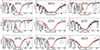 |
Fig. A.1. Damped H I-Ly-α lines for the proximate H2 systems. The X-shooter data are shown in black, and the profile corresponding to best fit is shown in red. The red shadows represent the conservative range of N(H I), including continuum placement uncertainties. There is residual Ly-α emission in the core of several DLAs. We also mark the expected position of the N Vλλ1238, 1242 doublet in blue. The tick marks represent the range seen in low-ionisation species (i.e. z5 and z95). It is here detected in all cases but J1259+0309 and J1331+0206. |
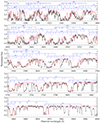 |
Fig. A.2. Portion of an X-shooter spectrum of J0019–0137 featuring H2 absorption bands. The solid red line shows the overall absorption model, and the contribution from non-H2 lines (H I, metals and lines from intervening systems) is shown as a dashed profile. The blue segments connect lines from different rotational levels (shown here for convenience from J = 0 to J = 5) of a given band (indicated by the label above, ’L’ for Lyman, ’W’ for Werner, and the following number is the upper vibrational level. |
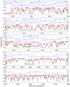 |
Fig. A.6. Same as Fig. A.2 for the quasar J1259+0309. A high-velocity broad absorption line (BAL) system lies in this quasar. |
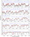 |
Fig. A.10. Same as Fig. A.2 for the quasar J2325+1539. |
Appendix B: Low-ionisation metal absorption lines
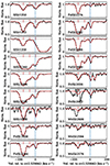 |
Fig. B.1. Main singly ionised metal lines in the proximate system towards J0019–0137 in their ground state. The zero of the velocity scale is set to the redshift of the H2 component (dashed blue line). Short red ticks mark the position of the different components used in the model (overplotted in red). |
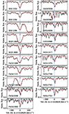 |
Fig. B.2. Singly ionised metal lines in the proximate system towards J0059+1124. |
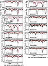 |
Fig. B.3. Singly ionised metal lines in the proximate system towards J1236+0010. The spike at v = 0 in Fe IIλ2382 is a sky-line residual. |
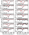 |
Fig. B.4. Singly ionised metal lines in the proximate system towards J1248+0639. |
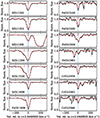 |
Fig. B.5. Singly ionised metal lines in the proximate system towards J1259+0309. |
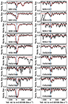 |
Fig. B.6. Singly ionised metal lines in the proximate system towards J1331+0206. |
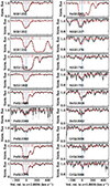 |
Fig. B.7. Singly ionised metal lines in the proximate system towards J1358+1410. |
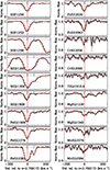 |
Fig. B.8. Singly ionised metal lines in the proximate system towards J2228-0221.. |
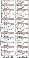 |
Fig. B.9. Singly ionised metal lines in the proximate system towards J2325+1539. Mn II is close to the sky residuals. |
 |
Fig. B.10. Neutral argon absorption lines. The dashed blue profile and dotted red and solid red represents the Ar I H2 and total absorption, respectively. The dashed green profile represents the expected total absorption obtained by scaling the S II profile assuming all argon to be in neutral form and a solar [Ar/S] ratio. The vertical dotted line shows the location of the H2 component. |
Results of Voigt-profile fitting to singly ionised metal absorption lines proximate to J0019–0137.
Results of Voigt-profile fitting to singly ionised metal absorption lines proximate to J0059+1124.
Results of Voigt-profile fitting to singly ionised metal absorption lines proximate to J1236+0010.
Results of Voigt-profile fitting to singly ionised metal absorption lines proximate to J1248+0639.
Results of Voigt-profile fitting to singly ionised metal absorption lines proximate to J1259+0309.
Results of Voigt-profile fitting to singly ionised metal absorption lines proximate to J1331+0206.
Results of Voigt-profile fitting to singly ionised metal absorption lines proximate to J1358+1410.
Results of Voigt-profile fitting to singly ionised metal absorption lines proximate to J2228-0221..
Results of Voigt-profile fitting to singly ionised metal absorption lines proximate to J2325+1539.
Appendix C: Measurement of dust extinction
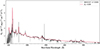 |
Fig. C.1. Measurement of the dust extinction by matching the X-shooter spectrum of J0019–0137 (black) with a reddened quasar composite spectrum from Selsing et al. (2016) (red). Grey regions were masked out during the fit. |
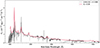 |
Fig. C.10. Same as Fig. C.1 for the quasar J1358+1410. |
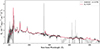 |
Fig. C.11. Same as Fig. C.1 for the quasar J2228-0221.. |
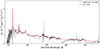 |
Fig. C.12. Same as Fig. C.1 for the quasar J2325+1539. |
Appendix D: Δv90 measurements
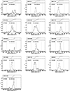 |
Fig. D.1. Measurements of Δv90 for low-ionisation line profiles. The different panels show the apparent optical depth (τ) in the selected transition line for a given system, and the cumulative apparent optical depth is shown on top. The segments represent the locations of the 5%, 50%, and 95% percentiles. |
Appendix E: Optical and NIR emission lines
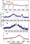 |
Fig. E.1. Emission lines from J0019–0137, detected in the visual and near-infrared. In the case of NIR, we show in dark grey the spectrum after iteratively rejecting deviant points. Blue dots show the median in 20-pixel bins. The best-fit model is shown by the solid red line. |
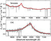 |
Fig. E.10. Same as Fig. E.1 for the quasar J2325+1539 |
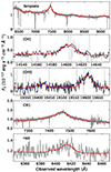 |
Fig. E.11. Same as Fig. E.1 for the quasar J1331+0206. |
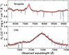 |
Fig. E.12. Same as Fig. E.1 for the quasar J2228-0221. |
Appendix F: CO(3-2) emission lines
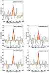 |
Fig. F.1. Detection of CO(3-2) emission from 3 mm NOEMA spectra extracted in 120 km s−1 bins. A single-component Gaussian fit is superimposed in red together with its 90% confidence interval. A sixth quasar (J0015+1842) in this sample has also been observed with NOEMA. The corresponding CO(3-2) detection was presented in Paper III. |
Results from Gaussian fits of CO(3-2) emission lines.
All Tables
Results of Voigt-profile fitting to singly ionised metal absorption lines proximate to J0019–0137.
Results of Voigt-profile fitting to singly ionised metal absorption lines proximate to J0059+1124.
Results of Voigt-profile fitting to singly ionised metal absorption lines proximate to J1236+0010.
Results of Voigt-profile fitting to singly ionised metal absorption lines proximate to J1248+0639.
Results of Voigt-profile fitting to singly ionised metal absorption lines proximate to J1259+0309.
Results of Voigt-profile fitting to singly ionised metal absorption lines proximate to J1331+0206.
Results of Voigt-profile fitting to singly ionised metal absorption lines proximate to J1358+1410.
Results of Voigt-profile fitting to singly ionised metal absorption lines proximate to J2228-0221..
Results of Voigt-profile fitting to singly ionised metal absorption lines proximate to J2325+1539.
All Figures
|
Fig. 1. Comparison of H2 (purple diamonds) and H I (green hexagons) column densities obtained using X-shooter and SDSS spectra. The dashed line depicts the one-to-one relation, and the dotted lines show ±0.3 dex around it. |
| In the text | |
|
Fig. 2. Observed abundance of sulphur against that of zinc in proximate H2 systems. |
| In the text | |
|
Fig. 3. Zinc-to-iron (bottom) and zinc-to-silicon (top) ratio for our sample of proximate H2 systems (circles with error bars). The colour scale provides the value of AV/N(H), which is a proxy of the dust-to-gas ratio. For two systems, the derived AV values are negative (hence unphysical) and the corresponding points are empty. Green triangles represent measurements in intervening DLAs (De Cia et al. 2016), and filled triangles correspond to known H2 intervening systems (Balashev et al. 2019). The solid blue lines show the best linear fit to the value for the proximate H2 systems, taking uncertainties on both axes into account. The green lines and shadowed region show the best linear fit and associated 1σ uncertainty for the overall sample of intervening DLAs. |
| In the text | |
|
Fig. 4. Dust-to-gas ratio measured from the continuum spectrum (filled circles) and derived from the metal column densities (open diamonds, following De Cia et al. 2016) as a function of depletion factor. The blue (purple) dotted line corresponds to a linear fit to ([Zn/Fe], log AV/N(H)) data points, where Av is based on continuum fitting (metal column density). |
| In the text | |
|
Fig. 5. Sulphur-to-silicon abundance ratio vs H I column density. The horizontal dashed line marks the solar ratio, and the vertical line shows the N(H I) limit below which Ellison et al. (2010) observed lower-than-solar abundances in PDLAs (see text). While not in our sample of proximate H2, one PDLA from Ellison et al. (2010), namely J2340-00, also has strong H2 and is marked with a blue circle. |
| In the text | |
|
Fig. 6. Sulphur-to-silicon vs zinc-to-iron abundance ratios in proximate H2 and DLA systems. The green line and shaded area represent the best fit for intervening DLAs by De Cia et al. (2016) and the 1σ scatter around this relation. The dashed blue line is a linear fit to the proximate H2 data. Dashed vertical and horizontal lines mark solar values. Symbols and colours for data points are as in Fig. 5. |
| In the text | |
|
Fig. 7. Observed [Ar/S] ratio (based on Ar I and S II) as a function of overall metallicity (top) and H I column density (bottom) in our sample of proximate systems. Blue circles correspond to the overall value in each system, and purple diamonds and red crosses show the H2 and non-H2 components, respectively. The dashed lines correspond to the corresponding mean values. The distribution is shown in the side panel. The green line corresponds to the mean [Ar/S] value (corrected to the same solar reference) and dispersion for intervening DLAs (Zafar et al. 2014b). Even though we tried to take blends into account, all points should be considered as upper limits in principle. |
| In the text | |
|
Fig. 8. Column density of molecular hydrogen vs total neutral hydrogen column density N(H I) = N(H I) + 2N(H2) for our sample of proximate H2 absorbers and z > 2 intervening strong H2-bearing DLAs from Balashev et al. (2019). For a fair comparison, we removed systems that may potentially be proximate, and kept only systems with a conservative cut of c (zabs − zQSO)/(1 + zQSO) < − 10 000 km s−1. Our selection of proximate H2 systems based on strong H2 lines directly seen in the low-resolution SDSS spectra naturally skews our sample to high H2 columns. The horizontal blue line shows the approximate and empirical lower limit of at log N(H2) > 18.5 for the present sample. The top histograms show the N(H) distributions for the proximate (blue) and intervening (green) systems with N(H2) > 18.5. Finally, the different lines correspond to different averaged molecular fractions fH2 ≡ 2N(H2)/2N(H2) + N(H I)). |
| In the text | |
|
Fig. 9. Metallicity vs total hydrogen column density. The different lines correspond to the hydrogen column density of a single H2 cloud illuminated by a UV field for different UV to density ratios IUV/n as indicated above each line, with IUV in units of the Draine field and n in cm−3. Filled symbols correspond to H2-bearing systems. Proximate H2 systems are from this work, proximate DLAs from Ellison et al. (2010), and intervening systems from Noterdaeme et al. (2008) and Balashev et al. (2019). |
| In the text | |
|
Fig. 10. Metallicity vs velocity extent of the low-ionisation metal lines for our sample of proximate H2 systems and a sample of intervening DLAs (mostly from Ledoux et al. 2006 with some additions by Noterdaeme et al. 2008). The green line shows the best-fit relation for high-z intervening DLAs by Ledoux et al. (2006). |
| In the text | |
|
Fig. 11. Summary of absorbing gas metallicity and kinematics. The differently coloured segments represent the Δv90 regions, and dots indicate the location of H2 components. The zero of the velocity scale is set to the best estimate of the systemic redshift zsys from ionised lines (Sect. 4.2). Positive velocities mean here |
| In the text | |
|
Fig. A.1. Damped H I-Ly-α lines for the proximate H2 systems. The X-shooter data are shown in black, and the profile corresponding to best fit is shown in red. The red shadows represent the conservative range of N(H I), including continuum placement uncertainties. There is residual Ly-α emission in the core of several DLAs. We also mark the expected position of the N Vλλ1238, 1242 doublet in blue. The tick marks represent the range seen in low-ionisation species (i.e. z5 and z95). It is here detected in all cases but J1259+0309 and J1331+0206. |
| In the text | |
|
Fig. A.2. Portion of an X-shooter spectrum of J0019–0137 featuring H2 absorption bands. The solid red line shows the overall absorption model, and the contribution from non-H2 lines (H I, metals and lines from intervening systems) is shown as a dashed profile. The blue segments connect lines from different rotational levels (shown here for convenience from J = 0 to J = 5) of a given band (indicated by the label above, ’L’ for Lyman, ’W’ for Werner, and the following number is the upper vibrational level. |
| In the text | |
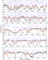 |
Fig. A.3. Same as Fig. A.2 for the quasar J0059+1124. |
| In the text | |
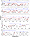 |
Fig. A.4. Same as Fig. A.2 for the quasar J1236+0010. |
| In the text | |
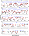 |
Fig. A.5. Same as Fig. A.2 for the quasar J1248+0639. |
| In the text | |
|
Fig. A.6. Same as Fig. A.2 for the quasar J1259+0309. A high-velocity broad absorption line (BAL) system lies in this quasar. |
| In the text | |
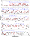 |
Fig. A.7. Same as Fig. A.2 for the quasar J1331+0206. |
| In the text | |
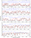 |
Fig. A.8. Same as Fig. A.2 for the quasar J1358+1410. |
| In the text | |
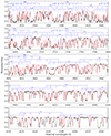 |
Fig. A.9. Same as Fig. A.2 for the quasar J2228-0221. |
| In the text | |
|
Fig. A.10. Same as Fig. A.2 for the quasar J2325+1539. |
| In the text | |
|
Fig. B.1. Main singly ionised metal lines in the proximate system towards J0019–0137 in their ground state. The zero of the velocity scale is set to the redshift of the H2 component (dashed blue line). Short red ticks mark the position of the different components used in the model (overplotted in red). |
| In the text | |
|
Fig. B.2. Singly ionised metal lines in the proximate system towards J0059+1124. |
| In the text | |
|
Fig. B.3. Singly ionised metal lines in the proximate system towards J1236+0010. The spike at v = 0 in Fe IIλ2382 is a sky-line residual. |
| In the text | |
|
Fig. B.4. Singly ionised metal lines in the proximate system towards J1248+0639. |
| In the text | |
|
Fig. B.5. Singly ionised metal lines in the proximate system towards J1259+0309. |
| In the text | |
|
Fig. B.6. Singly ionised metal lines in the proximate system towards J1331+0206. |
| In the text | |
|
Fig. B.7. Singly ionised metal lines in the proximate system towards J1358+1410. |
| In the text | |
|
Fig. B.8. Singly ionised metal lines in the proximate system towards J2228-0221.. |
| In the text | |
|
Fig. B.9. Singly ionised metal lines in the proximate system towards J2325+1539. Mn II is close to the sky residuals. |
| In the text | |
|
Fig. B.10. Neutral argon absorption lines. The dashed blue profile and dotted red and solid red represents the Ar I H2 and total absorption, respectively. The dashed green profile represents the expected total absorption obtained by scaling the S II profile assuming all argon to be in neutral form and a solar [Ar/S] ratio. The vertical dotted line shows the location of the H2 component. |
| In the text | |
|
Fig. C.1. Measurement of the dust extinction by matching the X-shooter spectrum of J0019–0137 (black) with a reddened quasar composite spectrum from Selsing et al. (2016) (red). Grey regions were masked out during the fit. |
| In the text | |
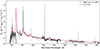 |
Fig. C.2. Same as Fig. C.1 for the quasar J0059+1124. |
| In the text | |
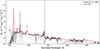 |
Fig. C.3. Same as Fig. C.1 for the quasar J0125–0129. |
| In the text | |
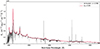 |
Fig. C.4. Same as Fig. C.1 for the quasar J0136+0440. |
| In the text | |
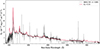 |
Fig. C.5. Same as Fig. C.1 for the quasar J0858+1749. |
| In the text | |
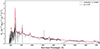 |
Fig. C.6. Same as Fig. C.1 for the quasar J1236+0010. |
| In the text | |
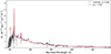 |
Fig. C.7. Same as Fig. C.1 for the quasar J1248+0639. |
| In the text | |
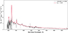 |
Fig. C.8. Same as Fig. C.1 for the quasar J1259+0309. |
| In the text | |
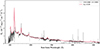 |
Fig. C.9. Same as Fig. C.1 for the quasar J1331+0206. |
| In the text | |
|
Fig. C.10. Same as Fig. C.1 for the quasar J1358+1410. |
| In the text | |
|
Fig. C.11. Same as Fig. C.1 for the quasar J2228-0221.. |
| In the text | |
|
Fig. C.12. Same as Fig. C.1 for the quasar J2325+1539. |
| In the text | |
|
Fig. D.1. Measurements of Δv90 for low-ionisation line profiles. The different panels show the apparent optical depth (τ) in the selected transition line for a given system, and the cumulative apparent optical depth is shown on top. The segments represent the locations of the 5%, 50%, and 95% percentiles. |
| In the text | |
|
Fig. E.1. Emission lines from J0019–0137, detected in the visual and near-infrared. In the case of NIR, we show in dark grey the spectrum after iteratively rejecting deviant points. Blue dots show the median in 20-pixel bins. The best-fit model is shown by the solid red line. |
| In the text | |
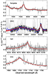 |
Fig. E.2. Same as Fig. E.1 for the quasar J0059+1124. |
| In the text | |
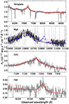 |
Fig. E.3. Same as Fig. E.1 for the quasar J0136+0440. |
| In the text | |
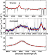 |
Fig. E.4. Same as Fig. E.1 for the quasar J0125–0129. |
| In the text | |
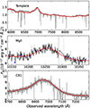 |
Fig. E.5. Same as Fig. E.5 for the quasar J0858+1749. |
| In the text | |
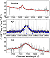 |
Fig. E.6. Same as Fig. E.1 for the quasar J1236+0010. |
| In the text | |
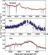 |
Fig. E.7. Same as Fig. E.1 for the quasar J1248+0639. |
| In the text | |
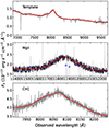 |
Fig. E.8. Same as Fig. E.1 for the quasar J1259+0309. |
| In the text | |
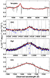 |
Fig. E.9. Same as Fig. E.1 for the quasar J1358+1410. |
| In the text | |
|
Fig. E.10. Same as Fig. E.1 for the quasar J2325+1539 |
| In the text | |
|
Fig. E.11. Same as Fig. E.1 for the quasar J1331+0206. |
| In the text | |
|
Fig. E.12. Same as Fig. E.1 for the quasar J2228-0221. |
| In the text | |
|
Fig. F.1. Detection of CO(3-2) emission from 3 mm NOEMA spectra extracted in 120 km s−1 bins. A single-component Gaussian fit is superimposed in red together with its 90% confidence interval. A sixth quasar (J0015+1842) in this sample has also been observed with NOEMA. The corresponding CO(3-2) detection was presented in Paper III. |
| In the text | |
Current usage metrics show cumulative count of Article Views (full-text article views including HTML views, PDF and ePub downloads, according to the available data) and Abstracts Views on Vision4Press platform.
Data correspond to usage on the plateform after 2015. The current usage metrics is available 48-96 hours after online publication and is updated daily on week days.
Initial download of the metrics may take a while.