| Issue |
A&A
Volume 694, February 2025
|
|
|---|---|---|
| Article Number | A294 | |
| Number of page(s) | 9 | |
| Section | Extragalactic astronomy | |
| DOI | https://doi.org/10.1051/0004-6361/202453387 | |
| Published online | 20 February 2025 | |
Exploring quasar evolution with proximate molecular absorbers: Insights from the kinematics of highly ionized nitrogen⋆
1
Departamento de Astronomía, Universidad de Chile, Casilla 36-D, Santiago, Chile
2
French-Chilean Laboratory for Astronomy, IRL 3386, CNRS and U. de Chile, Casilla 36-D, Santiago, Chile
3
Institut d’Astrophysique de Paris, CNRS-SU, UMR 7095, 98bis bd Arago, 75014 Paris, France
4
Ioffe Institute, Polyteknicheskaya 26, 194021 Saint-Petersburg, Russia
5
INAF – Osservatorio Astronomico di Trieste, Via G.B. Tiepolo, 11, I-34143 Trieste, Italy
6
Centre de Recherche Astrophysique de Lyon, UMR5574, U. Lyon 1, ENS de Lyon, CNRS, 69230 Saint-Genis-Laval, France
⋆⋆ Corresponding author; noterdaeme@iap.fr
Received:
11
December
2024
Accepted:
20
January
2025
We investigate the presence and kinematics of N V absorption proximate to high redshift quasars with both strong H2 and H I absorption at the quasar redshift. Our spectroscopic observations with X-shooter at the VLT reveal a 70% detection rate of N V (in 9 out of 13 quasars with 2.5 < z < 3.3), remarkably higher than the ∼10% detection rate in intervening damped Lyman-α systems and the ∼30% rate observed within a few thousand km s−1 of the source in the general quasar population. While many N V components lie within the velocity range of the neutral gas, the kinematic profiles of high-ionization species appear decoupled from those of low-ionization species, with the former extending over much larger velocity ranges, particularly toward bluer velocities (up to several thousand km s−1). We also observe significant variations in the N V to Si IV ratio, which we attribute to varying ionization conditions, with a clear velocity-dependent trend: blueshifted N V components systematically exhibit higher ionization parameters compared to those near the quasar’s systemic redshift. Furthermore, the most redshifted systems relative to the quasar show no evidence of N V absorption. The results suggest that proximate H2 absorption systems are in critical stages of quasar evolution, during which the quasar remains embedded in a rich molecular environment. Redshifted systems likely trace infalling gas, potentially associated with mergers, prior to the onset of outflows. Such outflows, as traced by N V, may eventually reach or even carry out neutral and molecular gas. This stage would correspond to proximate H2 systems located around or blueshifted relative to the quasar’s systemic redshift. Finally, the only case in our sample featuring highly blueshifted neutral gas (−2000 km s−1) shows no evidence of an association with the quasar. Our findings highlight the need to account for the ionization state when defining a velocity threshold to distinguish quasar-associated systems from intervening ones.
Key words: galaxies: active / galaxies: evolution / galaxies: general / quasars: absorption lines
© The Authors 2025
 Open Access article, published by EDP Sciences, under the terms of the Creative Commons Attribution License (https://creativecommons.org/licenses/by/4.0), which permits unrestricted use, distribution, and reproduction in any medium, provided the original work is properly cited.
This article is published in open access under the Subscribe to Open model. Subscribe to A&A to support open access publication.
1. Introduction
Understanding the coevolution of active galactic nuclei (AGNs) and their host galaxies is a major topic in astronomy (Volonteri et al. 2021; Morganti 2017). While the presence of the bright nucleus hinders observations of host and companion galaxies in emission, it becomes an advantage when studying the gas in absorption. For example, the presence of neutral gas along the line of sight with N(H I) ≥ 2 × 1020 cm−2 is revealed by the so-called damped Lyman-α systems (DLAs; see, e.g., Wolfe et al. 2005).
These systems can be classified into two primary categories, intervening and associated, depending on their origin with respect to the background sources. Intervening DLAs are fortuitous encounters that are not related with the sources themselves. The incidence, column density, and metallicity distribution of intervening DLAs indicate that they are closely connected with the overall population of galaxies (e.g., Prochaska et al. 2005; Pontzen et al. 2008; Krogager et al. 2017, 2020).
When the redshift of an absorption system lies within a few thousand km s−1 of the source’s emission redshift, it is better referred to as a “proximate” (Ellison et al. 2002, 2010; Prochaska et al. 2008a). While the proximity in velocity space is immediate, it remains nontrivial to determine whether a given proximate DLA (PDLA) originates in the AGN host galaxy, originates in its environment, or if it has any association with the source at all (e.g., Møller & Warren 1998)1. Statistically, the higher incidence of DLAs at small velocity separations from quasars aligns with the expected galaxy overdensity, despite the counteracting effect of the quasar’s intense radiation, which ionizes gas over large distances (the so-called proximity effect; Prochaska et al. 2008b).
There is also evidence from metal lines suggesting that PDLAs exhibit distinct characteristics compared to intervening systems (Fechner & Richter 2009; Ellison et al. 2010, 2011). Finley et al. (2013) also noted the presence of strong Ly-α emission in the saturated core of at least some PDLAs. The strength and width of this emission are most likely explained by the Ly-α emission from the quasar not being fully covered by the absorber, as opposed to much weaker emission due to in situ star formation as directly detected in a few intervening DLAs (e.g., Møller et al. 2004; Fynbo et al. 2010; Noterdaeme et al. 2012; Krogager et al. 2013; Ranjan et al. 2018) or statistically from stacking fiber spectra (e.g., Rahmani et al. 2010; Noterdaeme et al. 2014; Dharmender et al. 2024). Interestingly, this also revealed a potential bias against the identification of PDLAs since the most recognizable characteristic of DLAs is normally their zero flux level over a wide velocity range. A population of PDLAs where the damped core is almost completely filled with emission has indeed been identified, with a primary identification based on metal absorption lines (Fathivavsari et al. 2018; Fathivavsari 2020).
More recently, Noterdaeme et al. (2019, hereafter N19) discovered a population of molecular-rich PDLAs detected solely based on the Lyman-Werner absorption bands of H2 in Sloan Digital Sky Survey (SDSS) quasar spectra. Not only is the incidence of proximate H2 absorbers much higher than what is expected from intervening statistics, but H2 is a sensitive tool for investigating the physical conditions in the gas (e.g., Balashev et al. 2019, 2020; Klimenko & Balashev 2020; Kosenko et al. 2024). For example, it has been possible to use H2 together with excited atomic species to measure the distance between the absorbing gas and the quasar and to reveal an origin in a multiphase outflow (Noterdaeme et al. 2021a). Noterdaeme et al. (2023, N23 hereafter) recently presented the follow-up of a sample of 13 proximate H2 systems observed with X-shooter on the Very Large Telescope (VLT). The measurement of kinematics aided by precise measurements of the quasar’s systemic redshift (from near-IR lines and/or CO emission lines with NOrthern Extended Millimeter Array (NOEMA)) together with a study of chemical abundances provide evidence that these systems originated in the environment of the quasar.
Remarkably, N V absorption (i.e., four-times-ionized nitrogen, N4+) appears to be frequent in these PDLAs. This is particularly interesting since ionizing nitrogen to such a level requires an energy of 77.5 eV, which is not produced by stellar light (it falls off rapidly after the He II ionization energy at 54 eV). Indeed, N V is rarely seen in intervening DLAs but seems to be more common in metal absorption systems within 5000 km s−1 of quasars (Perrotta et al. 2016, 2018) and is hence a likely indication of physical proximity as well.
In this study we investigated the presence of N V absorption in greater depth by employing velocity decompositions of the profiles and the observation of associated Si IV. We present our sample in Sect. 2 and the measurements in Sect. 3. We explain the photoionization modeling we carried out to aid the interpretation of the observations in Sect. 4. The results are presented and discussed in Sect. 5, and we conclude in Sect. 7. We assume a flat Λ cold dark matter cosmology with HO = 68 km s−1 Mpc−1, ΩΛ = 0.69, and Ωm = 0.31 (Planck Collaboration XIII 2016). The column densities (N) are provided in units of cm−2.
2. Sample and detection statistics
Our sample consists of 13 high-redshift (2.5 < z < 3.3) proximate H2 systems from N19, observed at resolving power R ∼ 6000–10 000 with the European Southern Observatory (ESO) VLT X-shooter spectrograph (Vernet et al. 2011). The spectra were processed using the official ESOREX pipeline, version 3.5.3 (Modigliani et al. 2010), and line profiles were modeled through a standard multicomponent Voigt-profile fitting. We refer to N23 for comprehensive details on the selection criteria, observations, data reduction, and measurements of column densities for low-ionization ions, from which gas-phase metallicities were derived. The basic information is presented in Table 1.
Quasar sample and N V-detection summary.
We focused on highly ionized species, specifically N V and Si IV, and to some extent, C IV. These ions produce doublet lines conveniently located redward of the Ly-α emission in proximate systems, simplifying their detection and measurement. We clearly detected N V doublets in nine out of thirteen systems in our sample, yielding a ∼70% detection rate – significantly higher than the rates observed so far in intervening DLAs (∼13% reported by Fox et al. 2009), with similar detection limits (log N(N V) ∼ 13).
Using high-resolution spectra of nearly a hundred DLAs, Fox et al. (2009) reported a similar N V detection rate of 13% for both intervening systems (10/75) and proximate systems (2/16, within 5000 km s−1 of the quasar). This similarity, which contrasts with the expectation of an enhanced N V detection rate due to the hard radiation field near quasars, may indicate that the quasar’s radiation field actually dominates over a smaller velocity range than previously assumed: At a few thousand km s−1, most PDLAs in the literature may still be intervening systems rather than being located in the quasar’s immediate environment. For instance, at z ∼ 2 − 3, 3000 km s−1 in the Hubble flow corresponds to a distance of approximately 10 Mpc, where the quasar’s UV radiation field diminishes to the level of the metagalactic background.
Here, despite their original detection in low-resolution spectra (N19), which in principle allowed for large velocity shifts from the quasar, all but one2 H2-selected system in our sample lie within 1000 km s−1 of the quasar’s systemic redshift (N23). This suggests a stronger physical association with the quasar than what is seen in regular PDLAs (as in the sample by Fox et al. 2009), which could explain our higher N V-detection rate. Interestingly, we find that N V absorption can also appear at high velocities relative to neutral gas. Among the nine systems with N V detections, one shows components confined to the velocity range of low-ionization species, seven exhibit components both within and beyond this range, and one contains components exclusively at high velocity separations.
3. Data analysis
A main assert of the present work is the possibility to resolve the line profiles and hence to investigate how physical quantities vary along the kinematical profile, and in particular, whether high-ions components can have some degree of association with the neutral gas (at least probing the same object) or arise from a distinct phenomena. While coinciding absorption components across species do not guarantee co-spatiality, differing velocities between species indicate separate clouds, though they may still trace the same overarching structure.
We performed simultaneous multicomponent Voigt-profile fitting of the detected N Vλλ1238,1242, Si IVλλ1393,1402 and C IVλλ1548,1550 doublets using the Voigtfit code (Krogager 2018). This approach enabled us to determine the relative velocities, Doppler parameters (b), and column densities (N) for each component within the systems. Because C IV lines are strongly saturated in most cases, the derived column densities are generally highly uncertain. However, C IV remains useful to constrain the velocity structure and ionization, particularly in weaker components where N V is detected but Si IV is below the detection threshold. The Voigt-profile fits and the column densities in N V-bearing components are available in Appendix A.
In Fig. 1 we compare the N V/Si IV column density ratio derived from Voigt-profile fitting with that obtained pixel-by-pixel using the apparent optical depth method (Savage & Sembach 1991) for the quasar J0019−0137. Both methods yield consistent results and reveal significant variations in the N V/Si IV ratio across the profile. Notably, there is a tendency for higher ratios at velocities outside the bulk of the neutral gas, quantified by Δv90 – the velocity range encompassing 90% of the total optical depth of low-ionization species (from N23). While the apparent optical depth method offers simplicity and uniqueness, it is sensitive to signal-to-noise ratio and saturation effects (Fox et al. 2005), and it cannot effectively account for line blending. Since blending is evident in several other cases, we used the Voigt-profile-derived quantities for subsequent analysis, keeping in mind that, as in most absorption studies, the decomposition may not be unique.
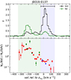 |
Fig. 1. Apparent optical depth and column density ratio toward J0019−0137. Top: Apparent optical depth of the N Vλλ1338 (green) and Si IVλλ1393 (black) absorption lines toward J0019−0137. The velocity extent of the low-ionization species (Δv90) is marked by the blue shaded region and the horizontal segment, with the tick marks corresponding to the 5, 50, and 95 percentiles of the cumulative optical depth (see Prochaska & Wolfe 1997). Bottom: Apparent column density ratio per unit velocity bin (red dots) and the ratio obtained for individual components used in the Voigt-profile modeling (stars). |
4. Photoionization models
To determine the physical origin of the variation in the N V-to-Si IV ratio, we performed photoionization models with Cloudy c.23 (last described in Chatzikos et al. 2023). We assumed a plane-parallel geometry of gas under a hard UV radiation field that is likely dominated by the quasar.
The incident radiation field is thus composed of the quasar radiation (“AGN field” in Cloudy), plus the metagalactic background taken from Khaire & Srianand (2019, KS19) at the redshift of the system. We checked that varying the adopted AGN field shape (following Vasudevan et al. 2009; Lusso et al. 2010; Meléndez et al. 2011; Del Moro et al. 2017), does not significantly affect the predicted column densities.
The incident flux in the model is represented in Fig. 2 over the relevant energy range for the present study. For the typical quasar luminosity ( L1450 = 1045.8 erg s−1 Å−1) in our sample, the incident UV field is dominated by the AGN up to about 1 Mpc, where it becomes comparable to the metagalactic background.
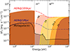 |
Fig. 2. Comparison of incident radiation fields. The metagalactic background (KS19), at redshift 2.6, is represented by the black line. The dashed red (blue) line represents the unattenuated AGN field, with the typical luminosity of our sample, at a distance of 100 kpc (1 Mpc). The other lines depict the transmitted flux through a H I layer with logarithmic column density values of 18 (pink), 19 (yellow), 20.3 (orange), and 21 (brown). The vertical dashed lines correspond to the ionization energy of hydrogen and that required to ionize nitrogen to N4+. |
Since we do observe strong damped Lyman-α absorption in our sample, we also show the effect of a H I layer on the transmitted radiation field, which becomes zero at 13.6 eV and only slowly recovers at higher energies. In the presence of neutral hydrogen, the number of available photons at energies above 77.5 eV –those capable of ionizing nitrogen to N4+– is drastically reduced at the DLA column density threshold. This indicates that the ionized gas containing N V is likely located upstream, closer to the quasar than the bulk of the neutral (H I-bearing) gas.
Since we have no direct measurement of the metallicity in the ionized phase, we used the metallicity from volatile species observed in the neutral phase (from N23) and assumed solar relative abundances (Grevesse et al. 2010). We note that a high-ionization phase might carry the bulk of the metals in an outflow. As a result, the low- and high-ionization phases may exhibit different metallicities. The assumed metallicity, however, has very little effect on the predicted column density ratios, since it results in an almost linear scaling of the column densities (Fig. B.1). As we will show later, this does not impact the derived ionization parameters. Because here we focused on ionized gas under the radiation field of the quasar, in which dust grains should be easily destroyed, we neglected dust-depletion.
An important unknown is the hydrogen column density of the clouds, to which the column densities of the metal species are directly scaled. For example, Perrotta et al. (2018) used a somehow arbitrary log N(H) = 20 as a stopping criterion when modeling the total integrated metal column densities. Here, since we have a measurement of the total H I column densities, one could be tempted to use the observed N(H I) as a stopping criterion. However, this approach would imply treating the full system as a single cloud, while in reality it certainly includes a mix of clouds and phases, as evidenced by the presence of multiple velocity components – in which we cannot determine the individual H I column density– and significant variations in observed N V/Si IV ratio between these components. Furthermore, the strong reduction of ionizing photons impedes the production of highly ionized species in the neutral gas, so that pushing the calculation to that depth would not bring any additional information on the ionized gas.
This is further illustrated in Fig. 3, which presents the calculated column densities of various species as a function of the ionization parameter U ≡ nγ/nH, where nγ is the number density of incident ionizing photons and nH the number density of hydrogen atoms, for different H I column densities and assuming the mean metallicity in our sample, log Z/Z⊙ = −0.9. As expected, the results concerning the highly ionized species are almost indistinguishable for log N(H I) = 18 and 21: despite us continuing the calculation up to three orders of magnitude higher H I column densities, no significant amounts of highly ionized metals are produced once we enter the H I-dominated regime. In contrast, the predicted column densities of Si IV, C IV and N V vary strongly between log N(H I) = 15 and 18. Solely from this calculation we observe that the detection of Si IV at the observed levels must imply a column density of log N(H I) > 15, since otherwise the predicted values do not exceed log N(Si IV) = 12 regardless of the ionizing parameter, contingent upon the assumed metallicity (here log Z/Z⊙ = −0.9). On the other hand, the detection of N V with column densities log N(N V) ∼ 12–16 implies ionization parameters likely above log U ∼ −2.5.
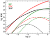 |
Fig. 3. Modeled column density of high-ionization species (color-coded) as a function of the ionization parameter for the different total H I column densities used as stopping criteria for the calculations. The models shown here were ran with log Z/Z⊙ = −0.9 (median metallicity of the sample) and log nH/cm−2 = 2. The dashed-dotted, dashed, and solid lines correspond to log N(H I) = 15, 18, and 21, respectively. |
In Fig. 4 we illustrate how the N V and Si IV column densities depend jointly on the ionization parameter and the H I column density. The metallicity is simply treated as direct scaling factor (see Fig. B.1). For values either below log N(H I) ∼ 17 or above log N(H I) ∼ 18, the N V–Si IV ratio depends primarily on the ionization parameter and is insensitive to the exact H I column density.
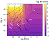 |
Fig. 4. N V/Si IV ratio (color scale) as a function of the ionization parameter and the H I column density in the cloud. The dashed green and dotted black lines represent the column densities of N V and Si IV scaled by the metallicity, i.e., log N(N V) − log Z/Z⊙ and log N(Si IV) − log Z/Z⊙. Crosses correspond to measurements in the individual components in our sample. Typical uncertainties on the observed column densities are about 0.2 dex. While these uncertainties are considered when inferring the U and N(H I) ranges, they are not represented here, to avoid overcrowding the figure. |
The dependence on the ionization parameter is, however, different in the low (log N(H I) < 17) and high (log N(H I) > 18) regimes. In the intermediate regime (i.e., crossing the H-ionization front), N V/Si IV depends strongly on both N(H I) and U. In Fig. 5 we present the same diagnostic diagram, but using C IV instead of Si IV. The overall behavior is very similar. Finally, we verified that for a given U, the models are almost insensitive to nH and nγ. Only their ratio matters.
5. Results
Based on our photoionization modeling, we located each component in the U–N(H I) plane using the measured N V and Si IV column densities (Figs. 4 and 5) and propagated their 1σ uncertainties accordingly. We assumed the metallicity to equal that of the PDLA system obtained from low-ionization metals. While this is in principle a strong assumption, a shift in metallicity translates into a shift in predicted N(H I) by the same factor, but has very little effect on the derived ionization parameter.
For weak components where N V is detected but Si IV is not, this approach provides lower limits on U. When feasible (i.e., for components that are neither saturated nor blended with stronger features), we then used C IV column density measurements instead of upper-limits on N(Si IV) to constrain the ionization parameter.
We find that no component occupies the high-N(H I) region in Fig. 4. A few components are near the ionization front, but the majority fall within the low N(H I) regime, well below log N(H I) = 17.5. In our overall sample, the three bluest N V components toward J0015+1842 have their expected Ly-α counterparts shifted outside the DLA trough. For these components, we directly confirm the low associated H I content, as shown in Fig. A.1.
A Voigt-profile fit, fixing the component’s positions, even yields log N(H I) = 13.7 ± 0.5, 13.2 ± 0.5, 14.2 ± 0.6, which remarkably agrees with the model predictions of 13.8, 13.6, and 14.8, especially given the metallicity dependence of these predicted values and the constraints based on only N V and C IV. The low H I columns naturally explains the lack of correspondence with low-ionization species, which are expected to arise in more shielded, high-N(H I) regions. This behaviour contrasts with the narrow N V components observed in the afterglow spectra of gamma-ray bursts (GRBs), which show little to no velocity shift relative to low-ionization metals. In GRB-DLAs, the highly ionized metals are more likely produced in the outer layers of dense clouds situated only a few parsecs from the progenitor star (Prochaska et al. 2008b).
Returning to proximate quasar systems, the N V column density alone would offer an initial indication of the ionization parameter, whereas Si IV does not (see Fig. 6). The N V/Si IV ratio, however, serves as a more reliable and robust proxy for the ionization parameter. It also eliminates dependences on metallicity and H I column density for log N(H I) ≲ 17. This relationship is approximately linear in log-space: log U ≈ 0.4 × log (N V/Si IV) − 2, offering a convenient diagnostic tool in the absence of detailed photoionization models, provided the H I column density remains low.
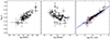 |
Fig. 6. Ionization parameter vs. column densities of N V, Si IV, and their ratio. Each point represents an individual N V-bearing component. Gray arrows represent limits on U for components where Si IV is not detected. The red and blue lines in the rightmost panel represent the model-predicted ratio for a fixed log N(H I) = 15 and a simple linear approximation (log U ≈ 0.4 × log (N V/Si IV) − 2), respectively. |
6. Discussion
With ionization parameter measurements now available for each component, an important question remains: the location and origin of the observed N V clouds. As previously argued, the N V components are likely located closer to the quasar than the first cloud exhibiting a significant H I column3 Additional insights can be obtained from the ionization stage and relative velocities of the components (see Fig. 7).
 |
Fig. 7. Ionization parameter vs. velocity of N V-bearing components with respect to the bulk of the neutral gas (left panel) or the quasar systemic redshift (right panel). Ionization parameters were derived from N V together with Si IV (circles and lower limits) or C IV (squares). The top panels show the velocity distribution of C IV (empty histograms) and N V (gray histograms) as well as subsamples created based on the derived ionization parameter. Some C IV components do not exhibit N V. In the left panel, points are color-coded according to the velocity normalized to that of the neutral gas, as used by Fox et al. (2007) to define whether a high-ionization component is likely gravitationally bound to the DLA (|v| < 2.4 Δv90) or not (see text). |
In the case of intervening DLAs, Fox et al. (2007) defined an escape velocity vesc ≃ 2.4Δvneutral, where Δvneutral is the velocity extent measured from absorption lines of singly ionized metals (i.e., taken here as Δv90). Components exceeding the escape velocity were interpreted as originating from winds. The left panel of Fig. 7 shows how the ionization parameter varies across velocity components for the entire sample, relative to the bulk of the neutral gas, and color-coded according to the criterion by Fox et al. 2007. To define the zero point of the velocity scale, we used z50 (Table 1), which corresponds to the redshift where the cumulative optical depth of low-ionization metals reaches 50% of its maximum value. This effectively represents the optical depth-weighted centroid of the neutral phase. We observe that the high-ionization profile extends over a significantly larger velocity range than the low-ionization profile and observe a pronounced asymmetry in the velocity distribution, characterized by a long tail extending toward blue velocities. Coupled with the likelihood that N V-bearing components are located upstream along the line of sight relative to the neutral gas, this asymmetry suggests that these components are moving away from the quasar, directed toward the bulk of the H I-absorbing gas.
This also raises the question of the persistence of N V in potential fast-moving outflows. The dynamical timescales corresponding to the motion of the absorbing gas can be estimated as tdyn = d/v, where v represents the velocity of the N V component (v < 3000 km s−1) and d is its distance from the AGN.
For the typical quasar luminosity in our sample, the distance can be estimated as d ∼ (109 cm−3/U/n)0.5 pc, resulting in tdyn > 1015(n/cm−3)−0.5 s for log U < −1, which is relevant to our studies. This timescale is significantly longer than the recombination timescale, trec ≈ 1011(n/cm−3)−1 s. In other words, the gas reflects the local ionization conditions.
In turn, the ionization state of the gas may or may not follow the AGN flickering or duty cycle, depending on its density (e.g., Rogantini et al. 2022). For example, under different assumptions: (i) for gas with n = 104 cm−3 (similar to broad absorption line outflows), located at ∼1 kpc (based on the AGN luminosity and log U = −1), the recombination time will be ≲1 yr, allowing the gas to follow any variations on timescales longer than this; (ii) for gas with n = 10−4 cm−3, akin to intergalactic medium conditions, the recombination time will be on the order of ≳10 Myr and the gas will only respond to variations on longer timescales. A more sophisticated time-dependent model would be required to fully capture these variations in the latter case.
Interestingly, Oppenheimer & Schaye (2013) emphasized that such fluctuations can significantly impact ions like N V, which may remain over-ionized for extended periods due to the slow recombination timescales of highly ionized species. This suggests that N V could serve as a tracer of past AGN activity, even after the ionizing source has faded. However, we lack precise knowledge of the gas number density or the AGN activity history, making it challenging to draw definitive conclusions. That said, the ionization parameters derived from our models likely represent characteristic conditions.
Additionally, N V can also be produced via collisional ionization in gas with temperatures around 105.3 ± 0.3 K, (where the ionization fraction peaks under collisional ionization Gnat & Sternberg 2007). These temperatures correspond to thermal b-parameters exceeding 15 km s−1, which may be inconsistent with the total width of many of the observed components. Our models also show that radiation from the nearby quasar is sufficient to reproduce the observed features, making it the simplest and preferred scenario.
We note that, despite the lower ionization potential of C IV that does not in principle require C IV to occur upstream with respect to the H I gas, the corresponding distribution is also skewed toward negative (blue) velocities. This suggests that, across our sample, these components are unlikely to originate from winds associated with an external galaxy (i.e., other than the quasar host). If this were the case, the velocity distribution would be expected to extend symmetrically also toward positive (red) velocities, as observed in intervening DLAs. In short, the highly ionized gas seen at significantly blue velocities with respect to the low-ionization metals are likely moving along the line of sight, from the quasar toward the bulk of the H I gas. Interestingly, we can see that the asymmetry in the velocity distribution remains present even when restricting to points within 2.4 × Δv90 (green in the figure), meaning that the escape velocity criterion by Fox et al. (2007) could also be too restrictive on average.
As we are examining quasar environments, it is interesting to analyze ionization as a function of velocity relative to the quasar’s systemic redshift, derived from the quasar emission lines (see N23), as illustrated in the right panel of Fig. 7. Interestingly, the C IV distribution now extends to redshifted velocities as well. This is primarily attributed to the three most redshifted DLAs (relative to the quasar), where the ionized gas more closely aligns with the neutral components in velocity space. However, the overall distribution of ionized (C IV) and highly ionized (N V) gas still shows a significant extent toward negative (blue) velocities. Additionally, it is noteworthy that subsamples defined by their ionization parameter reveal distinct velocity distributions: the highly ionized sample (with log U > −2) includes all components with v < −750 km s−1, while the sample with lower ionization (with log U < −2) shows components centered around zero velocity4.
We can generally expect that clouds with higher ionization parameters are more likely to be located closer to the quasar than those with lower U values. This is consistent with an origin in quasar outflows, where highly ionized gas exhibits high velocities near the quasar (see also Nestor et al. 2008; Balashev et al. 2023) and may eventually decelerates to the systemic velocity at greater distances, possibly when reaching the neutral gas, whose illuminated layer could also in principle produce N V.
All these considerations should be taken with caution as we are analyzing the sample as a whole. Figure 8 summarizes the ionization and velocity properties for each quasar individually. Based solely on the N V kinematics, one might interpret J0015+1842, J1358+1410, and J1331+0206 as exhibiting clear signatures of outflowing winds (high blueshifted velocities with high ionization). Indeed, a detailed study of J0015+1842 did reveal the presence of a multiphase, multi-scale outflow in that system (Noterdaeme et al. 2021a).
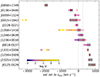 |
Fig. 8. PDLAs in our sample ordered according to the velocity difference between the centroid of the neutral gas (estimated from z50) and the systemic redshift of the quasar from optical emission lines. The dashed-dotted lines shows the typical velocity shift of the CO(3–2) emission in six systems observed with NOEMA, which may, on average, represent a better measurement of systemic redshift. The gray rectangles depict the low-ionization Δv90 range. Red crosses represent the position of H2 components. Diamonds represent N V components, colored according to the derived ionization parameter. |
The PDLA toward J0858+1749 is strongly blueshifted but lacks highly ionized gas. It is therefore plausible that this PDLA is an intervening system along the line of sight, and the −2000 km s−1 offset may originate from the Hubble flow. The presence of one such intervening system in our sample aligns with the observed excess of ∼10 − 20 times more H2 systems close to the quasar redshift compared to what is expected from intervening statistics (N19). This suggests that the velocity range used to associate a DLA with the quasar could be restricted to about ∼1000 km s−1 from the systemic redshift, while highly ionized gas can exhibit much larger velocities (see also Chen & Pan 2017, for similar conclusion from C IV and Mg II statistics).
Conversely, the three PDLAs with the most redshifted components show no evidence of N V. A comprehensive study involving X-shooter, Subaru Telescope (Subaru) and Atacama Large Millimeter/submillimeter Array (ALMA) data of one of them demonstrated that the absorption arises from a merging companion galaxy (Balashev et al. 2024).
Since molecular hydrogen and highly ionized nitrogen probe different phases and velocities relative to the quasar, one may wonder whether the presence of N V is related to the selection based on proximate H2 absorption. Based on a search among regular quasars, Perrotta et al. (2016) reached the same conclusion that N V are closely associated with the quasar and likely originating from outflowing gas. Interestingly, their study, also based on X-shooter data, revealed the presence of N V absorption in about a third of quasars (although about half of C IV absorbers within ±1000 km s−1 in their sample have also N V), when here the fraction is about twice higher. This result suggests that, although surprising, the selection based on H2 absorption appears to enhance the likelihood of detecting N V compared to the general quasar population. This excess in the N V detection rate is approximately 70% in H2 – bearing PDLAs, significantly higher than the 13% observed in intervening DLAs (Fox et al. 2009) and the roughly 30% found in regular quasars (Perrotta et al. 2016).
This may be an indirect effect: proximate H2 systems could select quasars surrounded by significant amounts of neutral and molecular gas, possibly witnessing the formation of these objects, as these are expected to be triggered by galaxy interactions and to feature strong outflows. In fact, the three H2 systems in our sample that have been studied in more details using ancillary data present remarkable properties: one is a possible post-merger system with a large reservoir of molecular gas with high velocity dispersion (Noterdaeme et al. 2021b), another lives in a rich galactic environment as traced by Ly-α emission (Urbina et al. 2024), and the third is part of a major merging system (Balashev et al. 2024). Additionally, 6 out of the 13 systems have been observed with NOEMA, resulting in six detections of CO(3–2) emission (N23).
Interestingly, the most redshifted PDLAs (likely tracing H I and H2 gas infalling toward the quasars) show no sign of outflow as indicated by the absence of N V absorption. This contrasts with the more blueshifted systems or those around the quasar systemic velocity, which do display clear outflow signatures. This suggests that while the highly ionized phase (N V) is decoupled from the H I phase, outflowing gas is primarily detected when PDLAs have velocities either moving toward the observer (blueshifted) or close to the quasar systemic velocity.
7. Conclusion
In this work we investigated the presence of four-times-ionized nitrogen (N V) in a sample of 13 quasars selected based on the detection of H2 absorption. A crucial aspect of our study was the use of medium-high-resolution spectroscopy, which enabled us to examine the properties of N V across the velocity profile. We confirm previous claims that N V is an effective tracer of quasar proximity (e.g., Ganguly et al. 2013; Perrotta et al. 2018) and quantified this by deriving the ionization parameter. Notably, we find higher ionization parameters in components at large blue velocity shifts from the quasar. We have also presented a straightforward and practical method for estimating this ionization parameter using the N V-to-Si IV ratio.
We conjecture that proximate H2 absorbers trace quasars during a key stage of their evolution, capturing the phase when galaxy interactions drive significant amounts of molecular gas toward the central engine, fueling it, while feedback in the form of outflows begins to expel gas outward. Whether the different properties observed in our sample are primarily due to evolutionary processes – such as a merger phase followed by outflows – or due to orientation, with infalling gas and outflows occurring in distinct directions, remains an open question. This underlines the need for more systematic and detailed studies of quasars with proximate H2 absorbers that examine not only the physical, chemical, and kinematical properties of the gas but also the emission characteristics of the quasars themselves and their surrounding galactic environments.
Data availability
Appendix A is publicly available on Zenodo: Zenodo repository link.
For these reasons, we favor “proximate” over “associated” (e.g., Weymann et al. 1979), traditionally defined by relative velocity alone, until a physical association is confirmed.
As we discuss later, the system with the largest velocity offset in our sample, at v ∼ −2000 km s−1 relative to quasar J0858+1749, lacks evidence of physical proximity and may instead represent an intervening system (see also Balashev et al. 2019).
Because of expected clustering around quasars, one might consider the possibility of a second AGN in the field, which could illuminate the gas from a different direction than assumed in the models. We therefore checked that no companion AGN is detected in SDSS in any of the studied field at least out to 200 pkpc at the redshift of the systems.
Acknowledgments
RC and PN gratefully acknowledge support from the French Chilean Laboratory for Astronomy. RC and SB are thankful to IAP for hospitality during part of the time this work was done, and so is PN with the Astronomy Departments of Universidad de Chile. SB is supported by RSF grant 23-12-00166. RC and SL acknowledges support by FONDECYT grant 1231187. The research leading to these results received support from the Agence Nationale de la Recherche, Project ANR-17-CE31-0011 “HIH2” (PI. Noterdaeme).
References
- Balashev, S. A., Klimenko, V. V., Noterdaeme, P., et al. 2019, MNRAS, 490, 2668 [NASA ADS] [CrossRef] [Google Scholar]
- Balashev, S. A., Ledoux, C., Noterdaeme, P., et al. 2020, MNRAS, 497, 1946 [NASA ADS] [CrossRef] [Google Scholar]
- Balashev, S. A., Ledoux, C., Noterdaeme, P., et al. 2023, MNRAS, 524, 5016 [NASA ADS] [CrossRef] [Google Scholar]
- Balashev, S. A., Noterdaeme, P., Gupta, N., et al. 2024, Nature, submitted [Google Scholar]
- Chatzikos, M., Bianchi, S., Camilloni, F., et al. 2023, Rev. Mexicana Astron. Astrofis., 59, 327 [Google Scholar]
- Chen, Z.-F., & Pan, D.-S. 2017, ApJ, 848, 79 [NASA ADS] [CrossRef] [Google Scholar]
- Del Moro, A., Alexander, D. M., Aird, J. A., et al. 2017, ApJ, 849, 57 [NASA ADS] [CrossRef] [Google Scholar]
- Dharmender, Joshi, R., Fumagalli, M., et al. 2024, A&A, 692, L7 [NASA ADS] [CrossRef] [EDP Sciences] [Google Scholar]
- Ellison, S. L., Yan, L., Hook, I. M., et al. 2002, A&A, 383, 91 [NASA ADS] [CrossRef] [EDP Sciences] [Google Scholar]
- Ellison, S. L., Prochaska, J. X., Hennawi, J., et al. 2010, MNRAS, 406, 1435 [NASA ADS] [Google Scholar]
- Ellison, S. L., Prochaska, J. X., & Mendel, J. T. 2011, MNRAS, 412, 448 [NASA ADS] [CrossRef] [Google Scholar]
- Fathivavsari, H. 2020, ApJ, 901, 123 [NASA ADS] [CrossRef] [Google Scholar]
- Fathivavsari, H., Petitjean, P., Jamialahmadi, N., et al. 2018, MNRAS, 477, 5625 [NASA ADS] [CrossRef] [Google Scholar]
- Fechner, C., & Richter, P. 2009, A&A, 496, 31 [NASA ADS] [CrossRef] [EDP Sciences] [Google Scholar]
- Finley, H., Petitjean, P., Pâris, I., et al. 2013, A&A, 558, A111 [NASA ADS] [CrossRef] [EDP Sciences] [Google Scholar]
- Fox, A. J., Savage, B. D., & Wakker, B. P. 2005, AJ, 130, 2418 [NASA ADS] [CrossRef] [Google Scholar]
- Fox, A. J., Petitjean, P., Ledoux, C., & Srianand, R. 2007, A&A, 465, 171 [NASA ADS] [CrossRef] [EDP Sciences] [Google Scholar]
- Fox, A. J., Prochaska, J. X., Ledoux, C., et al. 2009, A&A, 503, 731 [NASA ADS] [CrossRef] [EDP Sciences] [Google Scholar]
- Fynbo, J. P. U., Laursen, P., Ledoux, C., et al. 2010, MNRAS, 408, 2128 [NASA ADS] [CrossRef] [Google Scholar]
- Ganguly, R., Lynch, R. S., Charlton, J. C., et al. 2013, MNRAS, 435, 1233 [NASA ADS] [CrossRef] [Google Scholar]
- Gnat, O., & Sternberg, A. 2007, ApJS, 168, 213 [NASA ADS] [CrossRef] [Google Scholar]
- Grevesse, N., Asplund, M., Sauval, A. J., & Scott, P. 2010, Ap&SS, 328, 179 [Google Scholar]
- Khaire, V., & Srianand, R. 2019, MNRAS, 484, 4174 [NASA ADS] [CrossRef] [Google Scholar]
- Klimenko, V. V., & Balashev, S. A. 2020, MNRAS, 498, 1531 [CrossRef] [Google Scholar]
- Kosenko, D. N., Balashev, S. A., & Klimenko, V. V. 2024, MNRAS, 528, 5065 [NASA ADS] [CrossRef] [Google Scholar]
- Krogager, J.-K. 2018, VoigtFit: A Python package for Voigt profilefitting, ArXiv e-pints [arXiv:1803.01187] [Google Scholar]
- Krogager, J.-K., Fynbo, J. P. U., Ledoux, C., et al. 2013, MNRAS, 433, 3091 [NASA ADS] [CrossRef] [Google Scholar]
- Krogager, J. K., Møller, P., Fynbo, J. P. U., & Noterdaeme, P. 2017, MNRAS, 469, 2959 [NASA ADS] [CrossRef] [Google Scholar]
- Krogager, J.-K., Møller, P., Christensen, L. B., et al. 2020, MNRAS, 495, 3014 [NASA ADS] [CrossRef] [Google Scholar]
- Lusso, E., Comastri, A., Vignali, C., et al. 2010, A&A, 512, A34 [NASA ADS] [CrossRef] [EDP Sciences] [Google Scholar]
- Meléndez, M., Kraemer, S. B., Weaver, K. A., & Mushotzky, R. F. 2011, ApJ, 738, 6 [CrossRef] [Google Scholar]
- Modigliani, A., Goldoni, P., Royer, F., et al. 2010, in Observatory Operations: Strategies, Processes, and Systems III, Proc. SPIE, 7737, 773728 [Google Scholar]
- Møller, P., & Warren, S. J. 1998, MNRAS, 299, 661 [CrossRef] [Google Scholar]
- Møller, P., Fynbo, J. P. U., & Fall, S. M. 2004, A&A, 422, L33 [NASA ADS] [CrossRef] [EDP Sciences] [Google Scholar]
- Morganti, R. 2017, Front. Astron. Space Sci., 4, 42 [CrossRef] [Google Scholar]
- Nestor, D., Hamann, F., & Rodriguez Hidalgo, P. 2008, MNRAS, 386, 2055 [NASA ADS] [CrossRef] [Google Scholar]
- Noterdaeme, P., Petitjean, P., Carithers, W. C., et al. 2012, A&A, 547, L1 [NASA ADS] [CrossRef] [EDP Sciences] [Google Scholar]
- Noterdaeme, P., Petitjean, P., Pâris, I., et al. 2014, A&A, 566, A24 [NASA ADS] [CrossRef] [EDP Sciences] [Google Scholar]
- Noterdaeme, P., Balashev, S., Krogager, J. K., et al. 2019, A&A, 627, A32 [NASA ADS] [CrossRef] [EDP Sciences] [Google Scholar]
- Noterdaeme, P., Balashev, S., Krogager, J. K., et al. 2021a, A&A, 646, A108 [EDP Sciences] [Google Scholar]
- Noterdaeme, P., Balashev, S., Combes, F., et al. 2021b, A&A, 651, A17 [NASA ADS] [CrossRef] [EDP Sciences] [Google Scholar]
- Noterdaeme, P., Balashev, S., Cuellar, R., et al. 2023, A&A, 673, A89 [NASA ADS] [CrossRef] [EDP Sciences] [Google Scholar]
- Oppenheimer, B. D., & Schaye, J. 2013, MNRAS, 434, 1063 [NASA ADS] [CrossRef] [Google Scholar]
- Perrotta, S., D’Odorico, V., Prochaska, J. X., et al. 2016, MNRAS, 462, 3285 [NASA ADS] [CrossRef] [Google Scholar]
- Perrotta, S., D’Odorico, V., Hamann, F., et al. 2018, MNRAS, 481, 105 [NASA ADS] [CrossRef] [Google Scholar]
- Planck Collaboration XIII. 2016, A&A, 594, A13 [NASA ADS] [CrossRef] [EDP Sciences] [Google Scholar]
- Pontzen, A., Governato, F., Pettini, M., et al. 2008, MNRAS, 390, 1349 [NASA ADS] [Google Scholar]
- Prochaska, J. X., & Wolfe, A. M. 1997, ApJ, 487, 73 [NASA ADS] [CrossRef] [Google Scholar]
- Prochaska, J. X., Herbert-Fort, S., & Wolfe, A. M. 2005, ApJ, 635, 123 [NASA ADS] [CrossRef] [Google Scholar]
- Prochaska, J. X., Hennawi, J. F., & Herbert-Fort, S. 2008a, ApJ, 675, 1002 [Google Scholar]
- Prochaska, J. X., Chen, H.-W., Wolfe, A. M., Dessauges-Zavadsky, M., & Bloom, J. S. 2008b, ApJ, 672, 59 [NASA ADS] [CrossRef] [Google Scholar]
- Rahmani, H., Srianand, R., Noterdaeme, P., & Petitjean, P. 2010, MNRAS, 409, L59 [NASA ADS] [Google Scholar]
- Ranjan, A., Noterdaeme, P., Krogager, J. K., et al. 2018, A&A, 618, A184 [NASA ADS] [CrossRef] [EDP Sciences] [Google Scholar]
- Rogantini, D., Mehdipour, M., Kaastra, J., et al. 2022, ApJ, 940, 122 [NASA ADS] [CrossRef] [Google Scholar]
- Savage, B. D., & Sembach, K. R. 1991, ApJ, 379, 245 [NASA ADS] [CrossRef] [Google Scholar]
- Urbina, F., Noterdaeme, P., Berg, T. A. M., et al. 2024, A&A, 688, L25 [NASA ADS] [CrossRef] [EDP Sciences] [Google Scholar]
- Vasudevan, R. V., Mushotzky, R. F., Winter, L. M., & Fabian, A. C. 2009, MNRAS, 399, 1553 [NASA ADS] [CrossRef] [Google Scholar]
- Vernet, J., Dekker, H., D’Odorico, S., et al. 2011, A&A, 536, A105 [NASA ADS] [CrossRef] [EDP Sciences] [Google Scholar]
- Volonteri, M., Habouzit, M., & Colpi, M. 2021, Nat. Rev. Phys., 3, 732 [NASA ADS] [CrossRef] [Google Scholar]
- Weymann, R. J., Williams, R. E., Peterson, B. M., & Turnshek, D. A. 1979, ApJ, 234, 33 [NASA ADS] [CrossRef] [Google Scholar]
- Wolfe, A. M., Gawiser, E., & Prochaska, J. X. 2005, Annu. Rev. Astron. Astrophys., 43, 861 [CrossRef] [Google Scholar]
Appendix A: Fitting results
Appendix A is publicly available on Zenodo: Zenodo repository link.
Appendix B: Effect of the metallicity in the models
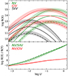 |
Fig. B.1. Predicted column density of N V, Si IV, and C IV (top) and the N V-to-Si IV and N V-to-C IV ratios (bottom) as a function of the ionization parameter. The solid lines correspond to the log N(H I) = 15 model in Fig. 3. The dashed (dashed-dotted) lines correspond to models that assume a ten-times-higher (lower) metallicity. The shaded areas show results from the central model (solid line), simply scaled up and down a posteriori by 1 dex. These scaled results match the predictions from the full calculations with corresponding metallicities reasonably well, typically within a factor of two (illustrated by the width of the stripes). |
All Tables
All Figures
|
Fig. 1. Apparent optical depth and column density ratio toward J0019−0137. Top: Apparent optical depth of the N Vλλ1338 (green) and Si IVλλ1393 (black) absorption lines toward J0019−0137. The velocity extent of the low-ionization species (Δv90) is marked by the blue shaded region and the horizontal segment, with the tick marks corresponding to the 5, 50, and 95 percentiles of the cumulative optical depth (see Prochaska & Wolfe 1997). Bottom: Apparent column density ratio per unit velocity bin (red dots) and the ratio obtained for individual components used in the Voigt-profile modeling (stars). |
| In the text | |
|
Fig. 2. Comparison of incident radiation fields. The metagalactic background (KS19), at redshift 2.6, is represented by the black line. The dashed red (blue) line represents the unattenuated AGN field, with the typical luminosity of our sample, at a distance of 100 kpc (1 Mpc). The other lines depict the transmitted flux through a H I layer with logarithmic column density values of 18 (pink), 19 (yellow), 20.3 (orange), and 21 (brown). The vertical dashed lines correspond to the ionization energy of hydrogen and that required to ionize nitrogen to N4+. |
| In the text | |
|
Fig. 3. Modeled column density of high-ionization species (color-coded) as a function of the ionization parameter for the different total H I column densities used as stopping criteria for the calculations. The models shown here were ran with log Z/Z⊙ = −0.9 (median metallicity of the sample) and log nH/cm−2 = 2. The dashed-dotted, dashed, and solid lines correspond to log N(H I) = 15, 18, and 21, respectively. |
| In the text | |
|
Fig. 4. N V/Si IV ratio (color scale) as a function of the ionization parameter and the H I column density in the cloud. The dashed green and dotted black lines represent the column densities of N V and Si IV scaled by the metallicity, i.e., log N(N V) − log Z/Z⊙ and log N(Si IV) − log Z/Z⊙. Crosses correspond to measurements in the individual components in our sample. Typical uncertainties on the observed column densities are about 0.2 dex. While these uncertainties are considered when inferring the U and N(H I) ranges, they are not represented here, to avoid overcrowding the figure. |
| In the text | |
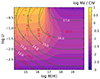 |
Fig. 5. Same as Fig. 4 but using N V (dashed green) and C IV (dotted red). |
| In the text | |
|
Fig. 6. Ionization parameter vs. column densities of N V, Si IV, and their ratio. Each point represents an individual N V-bearing component. Gray arrows represent limits on U for components where Si IV is not detected. The red and blue lines in the rightmost panel represent the model-predicted ratio for a fixed log N(H I) = 15 and a simple linear approximation (log U ≈ 0.4 × log (N V/Si IV) − 2), respectively. |
| In the text | |
|
Fig. 7. Ionization parameter vs. velocity of N V-bearing components with respect to the bulk of the neutral gas (left panel) or the quasar systemic redshift (right panel). Ionization parameters were derived from N V together with Si IV (circles and lower limits) or C IV (squares). The top panels show the velocity distribution of C IV (empty histograms) and N V (gray histograms) as well as subsamples created based on the derived ionization parameter. Some C IV components do not exhibit N V. In the left panel, points are color-coded according to the velocity normalized to that of the neutral gas, as used by Fox et al. (2007) to define whether a high-ionization component is likely gravitationally bound to the DLA (|v| < 2.4 Δv90) or not (see text). |
| In the text | |
|
Fig. 8. PDLAs in our sample ordered according to the velocity difference between the centroid of the neutral gas (estimated from z50) and the systemic redshift of the quasar from optical emission lines. The dashed-dotted lines shows the typical velocity shift of the CO(3–2) emission in six systems observed with NOEMA, which may, on average, represent a better measurement of systemic redshift. The gray rectangles depict the low-ionization Δv90 range. Red crosses represent the position of H2 components. Diamonds represent N V components, colored according to the derived ionization parameter. |
| In the text | |
|
Fig. B.1. Predicted column density of N V, Si IV, and C IV (top) and the N V-to-Si IV and N V-to-C IV ratios (bottom) as a function of the ionization parameter. The solid lines correspond to the log N(H I) = 15 model in Fig. 3. The dashed (dashed-dotted) lines correspond to models that assume a ten-times-higher (lower) metallicity. The shaded areas show results from the central model (solid line), simply scaled up and down a posteriori by 1 dex. These scaled results match the predictions from the full calculations with corresponding metallicities reasonably well, typically within a factor of two (illustrated by the width of the stripes). |
| In the text | |
Current usage metrics show cumulative count of Article Views (full-text article views including HTML views, PDF and ePub downloads, according to the available data) and Abstracts Views on Vision4Press platform.
Data correspond to usage on the plateform after 2015. The current usage metrics is available 48-96 hours after online publication and is updated daily on week days.
Initial download of the metrics may take a while.