| Issue |
A&A
Volume 669, January 2023
|
|
|---|---|---|
| Article Number | A145 | |
| Number of page(s) | 25 | |
| Section | Planets and planetary systems | |
| DOI | https://doi.org/10.1051/0004-6361/202244891 | |
| Published online | 26 January 2023 | |
ISPY: NACO Imaging Survey for Planets around Young stars
The demographics of forming planets embedded in protoplanetary disks★,★★
1
ETH Zurich, Institute for Particle Physics and Astrophysics,
Wolfgang-Pauli-Strasse 27,
8093
Zurich, Switzerland
2
Department of Astronomy, University of Michigan,
Ann Arbor, MI
48109, USA
e-mail: This email address is being protected from spambots. You need JavaScript enabled to view it.
3
Astrophysikalisches Institut und Universitätssternwarte, Friedrich-Schiller-Universität Jena,
Schillergs¨schen 2–3,
07745
Jena, Germany
4
Max-Planck-Institut für Astronomie,
Königstuhl 17,
69117
Heidelberg, Germany
5
Landessternwarte, Zentrum für Astronomie der Universität Heidelberg,
Königstuhl 12,
69117
Heidelberg, Germany
6
Observatoire Astronomique de l’Université de Genève,
51 Ch. des Maillettes,
1290
Versoix, Switzerland
7
Department of Physics, University of Warwick,
Gibbet Hill Road,
Coventry
CV4 7AL, UK
8
Centre for Exoplanets and Habitability, University of Warwick,
Gibbet Hill Road,
Coventry
CV4 7AL, UK
9
European Space Agency (ESA), ESA Office, Space Telescope Science Institute,
3700 San Martin Drive,
Baltimore, MD
21218, USA
Received:
6
September
2022
Accepted:
18
November
2022
Abstract
Context. Planet formation is a frequent process, but little observational constraints exist about the mechanisms involved, especially for giant planets at large separation. The NaCo-ISPY large program is a 120 night L′-band direct imaging survey aimed at investigating the giant planet population on wide orbits (a > 10 au) around stars hosting disks.
Aims. Here we present the statistical analysis of a subsample of 45 young stars surrounded by protoplanetary disks (PPDs). This is the largest imaging survey uniquely focused on PPDs to date. Our goal is to search for young forming companions embedded in the disk material and to constrain their occurrence rate in relation to the formation mechanism.
Methods. We used principal component analysis based point spread function subtraction techniques to reveal young companions forming in the disks. We calculated detection limits for our datasets and adopted a black-body model to derive temperature upper limits of potential forming planets. We then used Monte Carlo simulations to constrain the population of forming gas giant companions and compare our results to different types of formation scenarios.
Results. Our data revealed a new binary system (HD 38120) and a recently identified triple system with a brown dwarf companion orbiting a binary system (HD 101412), in addition to 12 known companions. Furthermore, we detected signals from 17 disks, two of which (HD 72106 and T CrA) were imaged for the first time. We reached median detection limits of L′ = 15.4 mag at 2″.0, which were used to investigate the temperature of potentially embedded forming companions. We can constrain the occurrence of forming planets with semi-major axis a in [20–500] au and Teff in [600–3000] K to be 21.2-13.6+24.3%, 14.8-9.6+17.5%, and 10.8-7.0+12.6% for Rp = 2, 3, 5 RJ, which is in line with the statistical results obtained for more evolved systems from other direct imaging surveys. These values are obtained under the assumption that extinction from circumstellar and circumplanetary material does not affect the companion signal, but we show the potential impact these factors might have on the detectability of forming objects.
Conclusions. The NaCo-ISPY data confirm that massive bright planets accreting at high rates are rare. More powerful instruments with better sensitivity in the near- to mid-infrared are likely required to unveil the wealth of forming planets sculpting the observed disk substructures.
Key words: planets and satellites: detection / planets and satellites: formation / protoplanetary disks
Residuals and contrast curves are only available at the CDS via anonymous ftp to cdsarc.cds.unistra.fr (130.79.128.5) or via https://cdsarc.cds.unistra.fr/viz-bin/cat/J/A+A/669/A145
Based on observations collected at the Paranal Observatory, ESO (Chile). Program ID: 097.C-0206(A), 097.C-0206(B), 198.C-0612(A), 198.C-0612(B), 198.C-0612(C), 199.C-0065(A), 199.C-0065(A2), 199.C-0065(B), 199.C-0065(C), 199.C-0065(D), 1101.C-0092(A), 1101.C-0092(C), 1101.C-0092(D), 1101.C-0092(E), 1101.C-0092(F), 1101.C-0092(G), 1101.C-0092(H).
© The Authors 2023
 Open Access article, published by EDP Sciences, under the terms of the Creative Commons Attribution License (https://creativecommons.org/licenses/by/4.0), which permits unrestricted use, distribution, and reproduction in any medium, provided the original work is properly cited.
This article is published in open access under the Subscribe-to-Open model. This email address is being protected from spambots. You need JavaScript enabled to view it. to support open access publication.
1 Introduction
In the last two and a half decades, more than 5000 extrasolar planets have been discovered. Their detection revealed a breathtaking diversity in their characteristics, such as mass, orbital separation, density, and atmospheric properties (e.g., Winn & Fabrycky 2015; Kaltenegger 2017; Madhusudhan 2019). Furthermore, we now know that planet formation is a very frequent and efficient process. Most of the known exoplanets have been discovered with transit and radial velocity (RV) surveys, and in the future many more will be revealed thanks to ongoing and future missions such as Gaia, which is expected to significantly contribute to the exoplanet inventory (e.g., Perryman et al. 2014; Gaia Collaboration 2023). These methods provide information on the planet demographics, but they are not able to put direct empirical constraints on their formation, as they suffer from observational biases that make observing young stars not ideal.
Complementary to the RV, astrometry, and transit techniques, direct imaging prefers young (i.e., brighter) planets well separated (a > 10 au) from their host star. In recent years, huge efforts and resources have been deployed to improve essential steps such as adaptive optics (AO) systems (e.g., Beuzit et al. 2019), coronagraphy (e.g., Martinache 2019), and postprocessing analysis (e.g., Cantalloube et al. 2020), which are indispensable to reach the high contrast necessary to image forming planets.
All of these investments brought several discoveries, including the iconic ß Pic system (Lagrange et al. 2009) and the HR8799 system, where at least four giant planets are orbiting the same star (Marois et al. 2008, 2010; Wang et al. 2018). Focusing on forming giant planets, several candidates were proposed in the past decade, but unfortunately most of them remain unconfirmed and under debate (e.g., LkCa15 b, HD 100546 b and c, and HD 169142 b; Sallum et al. 2015; Quanz et al. 2013; Reggiani et al. 2014, 2018; Biller et al. 2014; Rameau et al. 2017, to name a few). The first confirmed imaged forming planets have been PDS70 b (Keppler et al. 2018; Müller et al. 2018) and PDS70 c (Haffert et al. 2019). Since then, multiple studies to unveil their nature have been conducted (e.g., Bae et al. 2019; Stolker et al. 2020a; Wang et al. 2021; Cugno et al. 2021; Benisty et al. 2021). Finally, more recently, another protoplanet has been proposed around AB Aur using observations from multiple instruments over several years (Currie et al. 2022).
Direct imaging young, still forming planets is a particularly difficult, and yet important, task. Indeed, being embedded in the disk material, the planet flux is expected to suffer from extinction. Furthermore, high-contrast imaging post-processing techniques, especially angular differential imaging (ADI; Marois et al. 2006), might distort the disk scattered light morphology making it appear as point sources in the final residual images (e.g., Follette et al. 2017; Ligi et al. 2018). On the positive side, thermal emission from circumplanetary material is expected to contribute at longer wavelengths, potentially enhancing the possibility of a discovery (e.g., Zhu 2015). Despite these obstacles, detecting and studying forming planets will shed light on what are the main mechanisms that are driving planet formation, which formation model is expected to dominate (gravitational instability vs. core accretion; Boss 1997; Pollack et al. 1996), whether planets form following a hot-start, cold-start, or warmstart scenario (Marley et al. 2007; Spiegel & Burrows 2012; Mordasini et al. 2012), and where planets form with respect to their host star, potentially as a function of host star properties.
These are some of the questions that motivated the NaCo Imaging Survey for Planets around Young stars (NaCo-ISPY; Launhardt et al. 2020), an L′ imaging campaign at the Very Large Telescope (VLT) in Chile where we used 120 nights to investigate the population of gas giant planets around diskhosting stars. The ISPY targets can be divided into two different classes, debris disks (DEBs, 203 targets) and protoplanetary disks (PPDs, 50 targets).
While several other (larger) surveys tried and are trying to provide statistical constraints on the overall population of giant planets (e.g., Chauvin et al. 2010, 2015; Brandt et al. 2014; Stone et al. 2018; Nielsen et al. 2019; Vigan et al. 2021), NaCo-ISPY is unique in the sense that it only focuses on stars hosting a disk, trying to exploit this particularity while studying the potential interaction between disks and planets (Musso Barcucci et al. 2019; Pearce et al. 2022). A smaller survey with 15 targets and similar aims has been recently conducted with the VLT/SPHERE instrument by Asensio-Torres et al. (2021), unfortunately without detecting new planets. In Sect. 2 we present the sample of the survey, and in Sect. 3 we describe the observations, with the data reduction detailed in Sect. 4. Section 5 discusses results for individual targets, while Sect. 6 presents the statistical results of the survey as a whole. These results are discussed in Sect. 7 and we present our conclusions in Sect. 8.
2 Survey sample
2.1 Initial target list
The process of the target selection for the NaCo-ISPY survey has been detailed in Launhardt et al. (2020). As in this paper we only focus on the PPDs targets, we here provide some details on this subsample, and we refer to Launhardt et al. (2020) and Pearce et al. (2022) for information on the debris disk sample. In short, we compiled the initial target list from studies of Herbig Ae/Be stars (The et al. 1994; Menu et al. 2015), motivated by early detections of protoplanetary candidates orbiting those type of stars (e.g., Kraus & Ireland 2012; Quanz et al. 2013; Reggiani et al. 2014). These lists were complemented with additional objects hosting structured disks, which could indicate ongoing planet formation (e.g., ALMA Partnership et al. 2015; van Boekel et al. 2017; Konishi et al. 2016; Andrews et al. 2018; Avenhaus et al. 2018). Additional requirements were the target declination (−70° <Dec< +15°), distance (d < 1000 pc as measured at the time of compilation), multiplicity and K-band magnitude to ensure high quality AO correction (Launhardt et al. 2020). A total of 90 targets hosting a PPD were identified. We discarded 14 objects from our list because of existing L′ data or limited discovery space. Out of the 76 remaining targets, during the survey we observed 50 objects.
2.2 Sample properties
Targets of our sample are listed in Table A.1 and their parameter distributions are shown in Fig. 1. In the next paragraphs, we provide a top-level overview of these parameters, their source and their relevance for the ISPY search for forming planets.
Distances (top left panel of Fig. 1) were obtained from Gaia DR3 (Gaia Collaboration 2022) unless stated otherwise. Most of our targets have distance d < 200 pc, but some are much farther away.
L′ magnitudes (top right panel of Fig. 1) are obtained interpolating WISE photometry (Cutri 2013) between the W1 (3.35 µm) and W2 (4.6 µm) filters to the wavelength of our observations (3.8 µm). The vertical line in the L′ histogram represents the limit for the use of the Annular Groove Phase Mask (AGPM) coronagraph: for stars brighter than L′ ~ 6.5 mag we tried to use the coronagraph to increase contrast performance close to the star (see Sect. 3 for details about the observational setup). We note, however, that the final choice on the use of the coronagraph also depended on the weather conditions during the data acquisition.
Spectral types are taken from the SIMBAD database (Wenger et al. 2000), and span a wide range, from M3 to B5. Correspondingly, effective temperatures range from 3900 to 14000 K (middle left panel of Fig. 1; Launhardt et al. 2020; Pearce et al. 2022).
Stellar masses (middle right panel of Fig. 1) are taken from Kervella et al. (2019), but we used other literature values whenever unavailable. From other large direct imaging and ALMA surveys we know that massive stars have a higher chance to host giant planets (e.g., Vigan et al. 2021; Janson et al. 2021; Squicciarini et al. 2022) and massive disks (Andrews et al. 2013; Ansdell et al. 2016), which provide the building blocks to form planetary systems. Thus, it is a natural choice to focus on massive young Herbig Ae/Be stars in a survey such as NaCo-ISPY, and indeed almost all of our targets have masses M* ≳ 1 M⊙.
Stellar age is a crucial parameter for the interpretation of detection limits in high-contrast imaging data, as the magnitude to mass conversion strongly depends on the age assumption, especially for young targets. At the same time, age is one of the most difficult stellar parameters to constrain for young objects, with uncertainties and biases depending on the applied methods that dominate the measurements. We compiled stellar ages from the literature (see Table A.1), even though in Sect. 6 we constrain the population of forming protoplanets independently from age estimates.
2.3 Disks
A large fraction of our targets has been imaged with high resolution observations tracing the mm dust in thermal continuum, the scattering dust or the disk gas phase. Substructures in those components have been found to be ubiquitous. For example, rings, gaps and cavities are found in almost every disk imaged at sufficiently high resolution (e.g., Garufi et al. 2018; Andrews et al. 2018; Law et al. 2021). Hydrodynamical simulations (e.g., Zhu et al. 2012; Dipierro et al. 2016) indicate that they could be the result of protoplanets sculpting the disk material: indeed, young companions create gas pressure bumps able to stop dust radial drift and thus trap the dust in ring-like structures (e.g., Pinilla et al. 2015; Bae et al. 2018). Other commonly detected structures are spiral arms, which have been detected in several disks (Muto et al. 2012; Isella et al. 2018; Teague et al. 2019; Muro-Arena et al. 2020). Similarly to gaps, one of the most convincing explanations for their existence is the interaction with embedded planets (Fung & Dong 2015; Bae et al. 2016). Additionally, shadows have been observed in several disks (Stolker et al. 2017; Bohn et al. 2022; Teague et al. 2022), which could be caused by the presence of a warped unresolved inner disk that underwent dynamical interaction with a forming planet (Nealon et al. 2018). Despite the presence of forming planets being a very exciting explanation for all the disk substructures observed in the last decade, other mechanisms could be able to explain the disk observations and should be considered (e.g., Zhang et al. 2015; Birnstiel et al. 2015; Paneque-Carreño et al. 2021).
Given our goal of investigating the formation of planets in their natal protoplanetary disks, our search space is limited by the disk outer edge (see Table A.1). We used disk radii found in the literature from high angular resolution data obtained either with high contrast imagers or with ALMA and corrected for the newly measured distance from Gaia DR3. We confined our search region to a circular aperture from the central star with radius equal 1.5 × Rgas, where the factor 1.5 has been conservatively included to ensure that we are tracing the full radial extent of the disk and we do not reduce our search space because of low sensitivity observations. For some disks, measurements of Rgas do not exist, and we extrapolated the disk radius from measurements of the dust disk radius Rdust traced by the (sub)millimeter continuum emission. Several observational and theoretical studies indicate that gas in protoplanetary disks has a much larger extent than pebbles (e.g., Andrews et al. 2012; Isella et al. 2012; Birnstiel & Andrews 2014; Cleeves et al. 2016; Law et al. 2021; Zormpas et al. 2022). According to Trapman et al. (2019), the dichotomy in dust and gas sizes is due to a difference in optical depth between the two components (e.g., Facchini et al. 2017, who estimated Rgas/Rdust between ~1.4 and ~4 depending on the disk turbulence) and grain growth and subsequent radial drift (e.g., Natta et al. 2004; Ricci et al. 2010). Ansdell et al. (2018) investigated the relationship between sizes of the dust and gas components. They found gas-to-dust size ratios Rgas/Rdust between 1.5 and 3.5, with an average of 〈Rgas/Rdust〉 = 1.96 ± 0.04. Similarly, Long et al. (2022) estimated a 〈Rgas/Rdust〉 ratio of 2.9 ± 1.2 for 44 protoplanetary disks around stars with masses of 0.15–2.0 M⊙ and ages of 0.5–20 Myr. Trapman et al. (2019) estimated Rgas/Rdust using analytical models, and found that the ratio has a value usually between 1.5 and 3.5, if no dust evolution has already occurred. Based on these results, when only mm continuum measurements were available, we conservatively assumed a ratio of Rgas/Rdust = 3.5. A total of 20 targets (see Table A.1) do not have disk size measurements at all; in those cases we used the median of the measured disk sizes  au multiplied by 1.5. The distribution of disk radii for our targets is shown in the bottom left panel of Fig. 1 for the pebbles and the gas/µm-sized dust. As expected, the distributions indicate that overall Rdust < Rgas.
Disk inclinations are compiled from the literature (see references in Table A.1 and the bottom right panel of Fig. 1) with values obtained from spatially resolved high angular resolution imaging data. For two targets we imaged for the first time the disk ring in scattered light (HD 72106, TCrA), see Sect. 5.3. For those targets we estimated the disk inclinations, which are reported in Table A.1. Despite not being one of the main parameters used for target selection, disk inclination plays an important role in the detectability of planetary systems if one assumes that the orbital plane is coplanar with the protoplanetary disk. First, a highly inclined disk is very optically thick, preventing the light of the planet to escape. Second, a planet in a face-on disk is potentially always visible if it is above the contrast limits, while in an inclined disk, it will spend a considerable fraction of its orbit at smaller projected angular separations from the central star, in regions not accessible by the observations due to higher contrast and angular resolution requirements.
2.4 Additional target selection
To image and investigate the early phases of giant planet formation, we need access to a considerable fraction of the region occupied by protoplanetary disks. Too large stellar distances prevent us from inspecting the inner region of infant planetary systems because of the lack of spatial resolution. Furthermore, because the flux scales with 1/d2, the chances of a planetary mass companion to be detected are dramatically reduced for distant targets. Thus, we excluded from our sample 5 targets, as they have d > 500 pc (see Table A.1). Those targets, which are HD 85567, HD 259431, HD 95881, HD 98922 and HD 190073, were initially included in the sample because at the time of the compilation of the target list precise parallax measurements from Gaia were unavailable and they were thought to be much closer. As an example, the distance of HD 95881 was thought to be 170 ± 30 pc (Verhoeff et al. 2010), while Gaia locates the star at ~1110 pc. This additional cutoff leaves us with 45 targets analyzed in this paper. However, before discarding these targets we verified that no companion candidate nor disk signal were detected in the data following the procedure described in Sect. 4.
3 Observations
Data presented in this paper were taken between 2016 May 02 and 2019 May 25 using the AO-assisted NaCo imager (Rousset et al. 2003; Lenzen et al. 2003) with the L′ (λ = 3.8 µm) filter at the Very Large Telescope (VLT) at Paranal Observatory in Chile. Observations were carried out in Visitor Mode, and therefore some suffered from variable or bad weather conditions. In some cases, we opted for reobservation of the same system under better conditions, and here we only present the best available dataset for each target. Table A.2 reports the observations presented in this paper together with weather conditions.
All observations were taken in pupil-tracking mode to enable ADI, with field rotations depending on the elevation of the target and the integration time. We always tried to maximize the amount of rotation in the data in order to minimize self-subtraction effects when applying PSF-subtraction algorithms. For bright targets (L′ < 6.5 mag), we took advantage of the annular groove phase mask (AGPM) vector vortex coronagraph (Mawet et al. 2013) to further suppress stellar diffraction at small separations and improve the contrast. During these observations, the thermal background is sampled every 13 exposures by offsetting the sky position. For fainter targets (L′ > 6.5 mag), the AGPM could not be used as the star could not be properly centered behind the mask and we dithered the star for every cube (a cube is a collection of ~ 100–120 frames, depending on the dataset) on the three working quadrants of the L27 camera (pixel scale 0.027 mas pix−1)1. This sequence allows us to measure the background in the quadrant with the star before and after each exposure, which can be used to reconstruct the thermal contribution in each image.
At the beginning and at the end of each observing sequence, we took frames of the star without the coronagraph and with shorter exposure time to avoid saturation. Those frames are used to flux-calibrate each dataset. Thus, we made sure that unsatu-rated PSF images were particularly stable and, when necessary, we applied a strict manual selection to guarantee that variable weather conditions did not bias our results (see last column of Table A.2).
Figure 2 reports the most relevant properties of our observations. Overall, the median seeing was <1″.2 (panel a), with only two exceptions: V892 Tau and HD 100453 (see also Table A.2). Also, we note that for 19 targets, observations were executed with a median seeing ≲0″.6. The standard deviation of the seeing during each observation is reported in Table A.2 as well and can be interpreted as a measure for the stability of the atmosphere during the observing sequence. Given the relatively deep and long observations, and the fact that in most of the cases we planned observations in a period of the year with high sky rotation rate in the region of the target, we often achieved field rotations >60° (panel b). The third panel shows the time on target (ToT) we spent during our observations, which ranges between ~45 min and ~168 min. Several factors influenced the final ToT for each target, some of which beyond our control (e.g., weather conditions at Paranal or technical issues with the telescope and instrument). To measure the PSF stability, we estimated the flux for each unsaturated PSF frame enclosed in an aperture of r = 3.5 pix (~1 λ/D) around the image center. The standard deviation of the measured counts normalized to the median count gives a sense of the PSF stability (and thus photometric calibration) of our data. After removing bad frames (see Sect. 4.1.3), the PSF was very stable in most of the datasets, as shown in the panel d of Fig. 2.
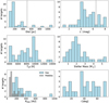 |
Fig. 1 Stellar and disk parameters for the objects in the ISPY PPD sample. In the top row the histogram for the distances (left) and L′ observed magnitudes (right) are reported. Stellar effective temperatures (left) and masses (right) are shown in the middle row. Finally, the bottom row provides the distributions of the disk outer radius (gas and mm-dust) on the left and disk inclinations (whenever measured) on the right. The dashed vertical lines represent the distance cutoff applied in Sect. 2.4 (top left panel) and the limiting brightness for the coronagraphic observations (top right panel), respectively. |
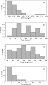 |
Fig. 2 Histograms reporting the weather conditions at the time of observations and key parameters describing the datasets. Panel a reports the DIMM seeing, panel b the field rotation, panel c the time spent on each target and panel d the PSF variation, respectively. |
4 Data reduction
The reduction of our data relies on PynPoint (Amara & Quanz 2012; Stolker et al. 2019), an end-to-end pipeline for reduction and analysis of high-contrast imaging data. Two different reduction flows were used for coronagraphic and noncoronagraphic datasets.
4.1 Preliminary reduction
4.1.1 Noncoronagraphic imaging
The data reduction for noncoronagraphic data follows that presented in Stolker et al. (2020a). Briefly, data were corrected for bad-pixels using 4σ clipping and substituting the bad pixels with the median of the eight surrounding pixels. The background is removed using the PCA-based algorithm described in Hunziker et al. (2018), where we benefit from the star hitting a different quadrant of the detector in each cube. Then, images are aligned to each other using a cross-correlation based algorithm and finally centered fitting a 2D Gaussian to the mean of all the images and shifting each image to locate the star at the very center. At this point, the images are cropped to a size that depends on the angular extent of the disk (Table A.1) as detailed in Sect. 2.3. Finally, we computed the counts in an aperture placed on the star of radius 1 pix and we discarded the frames whose values are more than 1–2 σ away from the mean depending on the stability of the PSF. This usually resulted in discarding <10% of the frames for each dataset. To reduce the amount of frames and frame-to-frame variations but at the same time keep enough features and diversity in the data, we always averaged over 20 consecutive frames in all datasets.
4.1.2 Coronagraphic imaging
The data reduction for coronagraphic imaging follows that presented in Cugno et al. (2019b). The initial ten frames of each cube suffered from a systematic offset that decreases exponentially to a constant level during the sequence (e.g., Stolker et al. 2019) and are therefore discarded to avoid biases during the background subtraction step. The remaining data are first corrected for bad-pixels as above, and subsequently the central star is identified with a 2D Gaussian. In some instances the fit failed, mainly because the AO loop briefly opened. Those frames are easily identified and removed by the frame selection routine later. Detector stripes are removed substituting bad pixels with the mean of the left and right pixels. Then, the background is removed using the median-collapsed offset sky cube taken after every 13 on-target cubes. When possible, the median between the previous and the next sky cubes is used. After background subtraction, the images are centered using the shifts previously registered, when we fit the PSF with 2D Gaussian models. Finally, the images are cropped in size based on the disk extent reported in Table A.1 and go through the same frame selection process. Again, the images were binned together every 20 frames.
4.1.3 Unsaturated PSF
The unsaturated images were obtained following the same observing and reduction strategy used for noncoronagraphic imaging data, in which the star was placed on three detector quadrants and the two empty quadrants were used to model and subtract the background. After undergoing the same frame selection as in Sect. 4.1.1 (strictly removing frames further than 1σ in this case), the images were median-combined to form a PSF model that could be used to calibrate the data.
4.2 PSF-subtraction
The stellar PSF was removed using full-frame principal components analysis (PCA, Amara & Quanz 2012; Soummer et al. 2012) as implemented in PynPoint using the median to combine the PSF-subtracted frames. Several hyperparameters could influence the final residuals, such as the number of the removed principal components (PCs) and the central mask applied to cover the very central pixels. To be able to study the innermost regions of protoplanetary disks, we applied a very small mask at the center of the image (r = 0″.05, i.e., ~2 pixels). Furthermore, we always removed between 1 and 40 components and inspected all the images. In this way we are able to evaluate more and less aggressive PCA setups, as different reductions are optimized for different regions of the images. For example, the same number of PCs might induce strong self-subtraction at small separations, while at the same time it might not remove enough stellar residuals at larger separations to reveal faint companions in protoplanetary disks. We note that, overall, most of the stellar signal was already removed after 20 components, leaving very clean residuals.
Bright companions, as is the case for binary systems, might dominate the PCs, leading to a poor PSF subtraction unable to reveal close-in planets. For this reason, an annular mask with a width of 4 λ/D at the separation of the binary star was applied, in order for the PCA to neglect the stellar companion and to focus on the region close to the primary.
We visually inspected all the images, searching for faint point sources from young companions. For nine objects, the residuals revealed bright binary system companions that required masking as described above. Once point sources were identified in the residuals, we proceeded with their characterization.
4.3 Companion characterization
We used two different methods in order to measure the astrometry and the photometry of companion candidates. The fifth column of Table 1 indicates which of the two methods was used to infer the properties of the companions.
For point sources in the speckle dominated region of the images (p ≲ 1″.0), we used the MCMC sampling algorithm provided in PynPoint, which inserts artificial negative copies of the unsaturated PSF in the images prior to the PCA PSF-subtraction step. Then, the central star was removed, and the residuals at the position of the companion were evaluated in an aperture of size r ≈ 2λ/D following the method described in Wertz et al. (2017). The posterior distribution for the three parameters separation, position angle (PA), and contrast was sampled with 300 walkers undergoing chains of 500 steps. For each walker, the first 100 samples are discarded as burn-in phase. Then, the best-fit companion is removed from the images and additional sources with the same contrast are inserted at the same separation as the original one, but with 360 different position angles. Those artificial companions are retrieved so that we could estimate potential biases in our measurement methods. Thus, we correct for the aforementioned bias and we added in quadrature the standard deviation of the 360 retrieved values to the measurement uncertainty. A more detailed description of this approach can be found in Stolker et al. (2020b).
For companions with ρ ≳ 1″.0 we ran classical ADI (cADI) to reduce self-subtraction and fitted the companion PSF with a 2D Gaussian function. The peak position is used to determine the astrometry of the companion, while the contrast is estimated comparing the amplitude of the fit with the amplitude of the unsaturated PSF after correcting for differences in exposure times. In this case we conservatively considered fixed uncertainties of 9 mas for both RA and DEC coordinates, as this was the total uncertainty on the separation that we measured for HD 101412 C (see Table 1 and Sect. 5.1.2) and it is unlikely that the Gaussian fitting method carries a larger uncertainties than those measured in the speckle dominated region at 0″.17. The uncertainties on the contrast are calculated assuming an error equal to the variability of the PSF (Table A.2).
Finally, for both methods separations and position angles were corrected using the plate scale and the true north corrections estimated in Launhardt et al. (2020). We report the final values in Table 1.
Full list of stellar and substellar companions detected in the NaCo-ISPY PPD sample.
4.4 Contrast curves
We calculated contrast curves for all data sets in the survey using applefy, which follows the routine presented in Bonse et al. (2022). Our analysis starts with a preparatory examination of residual noise statistics. For this purpose, we compute Q-Q plots to compare the pixel noise in the residuals with Gaussian noise. Exemplary results for HD 31648 and HD 36112 are given in Appendix C. The residual noise in areas which do not contain extended scattered light signals from a protoplanetary disk is mostly consistent with Gaussian noise. Although Q-Q plots cannot prove that the actual noise originates from a Gaussian distribution, we assume that the noise is sufficiently normal to perform a t-test (Mawet et al. 2014). On the contrary, in areas of our images which contain extended scattered light from a protoplanetary disk the statistic is dominated by the disk signal. In those regions, the noise is not normal (see right panel of Fig. C.1), and the noise can neither be considered independent (due to the extended nature of the disk signal) nor identically distributed (given that some areas are related to the disk signal, some to the dark regions originating from self-subtraction, and some are estimates of the true speckle and detector noise). Hence, none of the assumption necessary to compute detection limits based on the t-test (Mawet et al. 2014) is applicable. As a consequence, we exclude these regions from our analysis (usually the first few λ/D). This problem is limited to the innermost region of 17 targets (see Sect. 5.3), while the outer disk is never detected in scattered light in L′. For these 17 sources we started calculating contrast curves from the first fixed separation not including disk signals (see below) and we ignored regions at smaller separations.
The calculation of the contrast curves relies on three main components: the detection threshold, the signal of the planet and the strength of the noise. We fix the detection threshold to a false-positive-fraction (FPF) of 2.87 × 10⁻⁷ for all separations, which is equivalent to 5σ for large separations. We inject fake planets at different separations from the star (steps of 1λ/D at separations lower than 12 λ/D, steps of 3λ/D at larger separations as the contrast is expected to stabilize) using the unsaturated PSF. In this way we can calculate the attenuation of the planetary signal caused by over- and self-subtraction during the data post-processing. In order to account for azimuthal variations, 6 planets (one planet at a time) are inserted for every separation. The result is the throughput of the data post-processing as a function of separation averaged over 6 azimuthal positions. In contrast to the metric presented in Mawet et al. (2014), we do not use apertures but pixel values spaced by 1 FWHM (Bonse et al. 2022). In this way, the noise is approximately uncorrelated, which is a prerequisite for use of the t-test. For every separation we extract the noise for 360 different placements and report the median over all results.
5 Results on individual objects
Residuals on each individual target are shown in Figs. B.1–B.3. There, companions and concrete candidates are highlighted with circles, while nondetections of known companions at locations predicted by previous studies are marked with dashed circles. In Sect. 5.1 we focus on newly detected companions, in Sect. 5.2 we introduce interesting upper limits on individual undetected companions whose presence has been inferred with both direct and indirect methods, and in Sect. 5.3 we present the detection of disk signals. In Appendix D we describe the detection of known stellar and substellar companions, while in Appendix E we report the detection of background objects. A list of all the detected companions, together with their properties can be found in Table 1.
5.1 Newly detected companions around individual objects
5.1.1 HD 38120
The image of HD 38120 shows residuals from a companion candidate at the edge of the field of view (Fig. B.1). For this reason, we enlarged it by 0″.5 in radius, to include the signal coming from the potential companion. The companion candidate is detected at a separation of 1″.265 with a contrast of 0.4 mag. Having similar brightness in the L images, it is unlikely that the companion candidate is a background object. Nonetheless, we reduced archival NaCo data in the Ks-band (Prog. ID: 076.C-0679(B), PI: Bouwman) taken in 2006 in order to verify that the two objects are comoving. The proper motion analysis is reported in Fig. 3, showing that the candidate motion is inconsistent with a background object.
We further test the binary scenario by checking whether the candidate motion is consistent with a bound object, using the method of Pearce et al. (2015). Their parameter B (Eq. (1) in that paper) combines sky-plane separation, relative velocity and mass to assess whether two objects can be bound; if B < 1 then bound companionship is possible (although not certain, because the line-of-sight coordinates are unknown), whilst if B ≥ 1 then companionship is ruled out because the relative velocity would be too high (regardless of line-of-sight coordinates). We calculate B for HD 38120 using the 2006 and 2017 data (separated by 11.8 yr), for which the separations are 1″.242 ± 0″.009 and 1″.265 ± 0″.013 and the position angles 130.4 ± 0.4° and 128.6 ± 0.4° respectively (assuming uncertainties of one-third of a pixel, see Sect. 4.3). We use a primary mass of 2.6 ± 0.1 M⊙, and assume that the secondary has the same mass with a 100 percent uncertainty (since the contrast in L′ is only 0.4 mag). These yield B = 2.6 ± 2.0; it is therefore possible that B < 1 (within the uncertainties), and so it is dynamically possible for the pair to be bound. Reducing the uncertainty on the secondary mass would not change this conclusion.
5.1.2 HD 101412
Two new companions have been discovered around HD 101412 in our L′ images within 0″.6 from the primary. The study of the proper motion analysis, together with the companions classification performed with multiwavelength follow-up observations will be presented in a separate manuscript (Ruh et al., in prep.), while here we only report astrometric and photometric properties measured in the L′-band. We note that Rich et al. (2022) detected the same objects in GPI H-band data, and they assessed with 3σ confidence that the point sources are not background objects, in agreement with Ruh et al. (in prep.).
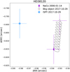 |
Fig. 3 Proper motion analysis of the stellar companion candidate orbiting HD 38120. The companion motion is inconsistent with a background object, and consistent with being bound. The dark diamond and circle are the 2006 and 2017 positions respectively, the solid line is the expected motion of a background object and the faded diamond is the expected position of a background object in 2017. |
5.2 Interesting nondetections and dubious candidates
5.2.1 HD 97048
Pinte et al. (2019) identified a kink in the isovelocity curve of HD 97048 at a separation corresponding to one of the dust gaps from the disk (ρ = 0″.45 ± 0″.1, PA = −55 ± 10°, Mp = 2−3 MJ). The NaCo images do not reveal a signal corresponding to that position, at which we reached a contrast of ~7.9 mag. Using the information provided in Table A.1, we estimate a mass upper limit of ~52 MJ using the Ames-Dusty evolutionary models (Chabrier et al. 2000). Much deeper observations will be necessary to unveil the companion in the dust gap.
5.2.2 HD 100546
Quanz et al. (2013) claimed the detection of a protoplanet ~47 ± 4 au away from the Herbig Ae/Be star HD 100546 using L′ data from VLT/NaCo. They confirmed the detection with a second independent L′ dataset (Quanz et al. 2015a), detected it in the M′-band as well, and used Ks-band data to put an upper limit on the companion flux at shorter wavelengths. Fitting the few available datapoints, Quanz et al. (2015a) concluded that they detected emission from the hot circumplanetary environment rather than from b itself. Furthermore, Currie et al. (2014, 2015) identified the planet b in GPI H-band data, confirming the very red IR colors, as expected for an embedded object. More recent works cast doubts on the existence of the protoplanet, suggesting that the detections are the result of scattered light from the disk after aggressive post-processing (Garufi et al. 2016; Follette et al. 2017; Rameau et al. 2017). Finally, Mendigutía et al. (2017) and Cugno et al. (2019a) searched for Hα signals emitted from the accretion shock surface without finding any.
The ISPY data revealed a potential point source at the position of HD 100546 b, best visible with relatively aggressive reductions obtained with a high number of principal components. However, the feature seems to have an elongated shape and it sits on a bright disk arm, as noted by Quanz et al. (2013) and Quanz et al. (2015a). Given the rather debated nature of HD 100546 b, this dataset will be studied in a separate paper focused uniquely on this object, and we do not consider it to be a confirmed companion in this study.
5.2.3 HD 142527
HD 142527 hosts a disk with a very large optically thin cavity. An accreting stellar companion is located within the cavity (Biller et al. 2012; Close et al. 2014) at ~0″.063 (Cugno et al. 2019a; Balmer et al. 2022) on an orbit misaligned with the outer disk (Lacour et al. 2016; Balmer et al. 2022). Being so close to its host, HD 142527 B falls at a separation smaller than the angular resolution of our NaCo observations (λ/D ≈ 0″.095). Hence, we did not detect it.
5.2.4 HD 163296
Pinte et al. (2018) inspected channel maps of the disk around HD 163296, identifying a kink in the velocity field of the disk gas, presumably caused by the presence of a forming companion with mass ~2 MJ. The planet was later independently confirmed by Teague et al. (2021) and Izquierdo et al. (2022) at a separation of ~2″.0 with PA ~ 0°. Our ISPY observation did not directly show the embedded companion, and at the expected companion separation we reached a contrast of 11.8 mag, corresponding to a limit on the brightness of the planet of 15.3 mag. Assuming that the emission is due to photospheric emission only (no accretion) and that the disk material does not influence at all the emitted flux, we can compare this value with the expected value from the hot-start Ames-Dusty evolutionary models (Chabrier et al. 2000, as used by Asensio-Torres et al. 2021) for a planet coeval with the parent star (7.1 Myr, see Table A.1). In this framework of assumptions, the detection limits exclude planet masses larger than ~4.2 MJ, consistent with our nondetection of HD 163296 b. We also note that our contrast curve is roughly consistent with that obtained by Guidi et al. (2018) with Keck/NIRC2 after correcting for the different statistical significance. Deeper observations, potentially with JWST, are necessary to confirm the indirect detection by Pinte et al. (2018).
5.3 Disks
Even if our observational strategy and reduction pipeline were not optimized for the detection of protoplanetary disk signals, 17 protoplanetary disks could be detected in the final residuals out of the 45 targets we observed with the VLT/NaCo instrument. For all these sources, the disk detections are reported in Fig. 4. Most of the disks from Fig. 4 were already known and images were taken in the past either with high-contrast imagers or with the ALMA observatory. Some of these disks were also already imaged in the L′-band. These are HD 34282 (Godoy et al. 2022; Quiroz et al. 2022), HD 36112 (Reggiani et al. 2018; Wagner et al. 2019), HD 36910 (Uyama et al. 2020), HD 100453 (Wagner et al. 2018), HD 100546 (Quanz et al. 2013, 2015a), PDS70 (Keppler et al. 2018; Wang et al. 2020; Stolker et al. 2020a), HD 141569 (Mawet et al. 2017), HD 142527 (Rameau et al. 2012), and HD 163296 (Guidi et al. 2018).
For other targets the first L’ disk images are reported in this work (some were already introduced in Launhardt et al. 2020, as part of an introduction to the ISPY survey). These are HD 58647 and V892 Tau (Stapper et al. 2022 presented ALMA images for these sources), MY Lup (previously imaged by Avenhaus et al. 2018 with VLT/SPHERE in polarimetric mode), TYC 7851-810-1 (imaged with ALMA by Ansdell et al. 2018), HD 152404 (Janson et al. 2016 showed SPHERE/IRDIS images of the disk) and HD 179218 (see also Kluska et al. 2018 and their VLT/SPHERE observations). Finally, to our knowledge this is the first direct detection of the disks surrounding HD 72106 and T CrA.
A coherent and exhaustive analysis of the disk images involves the study of the disk at other wavelengths, coupled with a radiative transfer code and assumption on the dust and gas distribution and properties. This is beyond the scope of this work, and we leave the interpretation of the disk signals to future work. However, in the next paragraph, we use the ellipse fitting tool from Hammel & Sullivan-Molina (2020) to derive at least some of the basic parameters of the newly discovered disks, especially the inclination that we subsequently use in Sect. 6.4.
First, we produce radial profiles in every 3° azimuth section and find the peak positions of the ring-like emission. To compensate for the coarse sampling of the disk near the major axis we sample every 1° near that region. The peak pixel coordinates are provided as input to the ellipse fitting routine. For each target, we perform the fitting on multiple images obtained by subtracting different numbers of components. The final values result from the average and the standard deviation of these separate fittings. The inclination is estimated from the aspect ratio assuming that the disk is a circle if seen face-on.
Given the geometrical similarities between the disks around HD 72106 and TCrA and the disk around TYC 7851-810-1, we used the latter to verify our procedure. The fit results i = 72 ± 3°, PA = 105 ± 2° are consistent with literature values i = 74° and PA =107° from Ansdell et al. (2018). We derive for HD 72106 a disk inclination i = 51 ± 4° and for TCrA i = 77 ± 2°. In addition, we obtain the position angle of the major axis PA = 47 ± 2°, and ring radius R = 70 ± 2 au for HD 72106, PA = 5 ± 2°, and R = 35 ± 2 au for T CrA. Inclinations are reported in Table A.1.
6 Results on the overall sample
In this Section we aim to interpret the results of our survey as a whole, drawing conclusions that can statistically constrain the population of forming planets. In Sect. 6.1 we look at the detection limits of our targets, in Sect. 6.2 we lay out several issues related to the transformation of detection limits into mass upper limits and we propose a solution in Sect. 6.3. Finally, in Sect 6.4 we compute completeness maps for the ISPY PPD survey.
6.1 Contrast and detection limits for the ISPY PPD sample
Figure 5 shows in gray the contrast curves obtained by applying the procedures described in Sect. 4.4 on each of the datasets presented in this paper. In addition, thick red lines show the median contrast obtained at each separation. The contrast performance of the WLY2–48 and KK Oph datasets are much worse than for the rest of the targets due to problems with the AO loop stability occurring during the observations (WLY2–48) and the presence of an equal brightness companion in the image that dominates the residuals (KK Oph). As discussed in Sect. 4.4, each contrast curve might have a different starting separation depending on the presence of a bright disk in scattered light preventing a reliable quantification of the FPF = 2.87 × 10⁻⁷ contrast at small separation, and a different radial extent depending on the radius of the protoplanetary disk surrounding the target. Thus, the number of contrast curves contributing to the median estimate at each separation may vary.
Overall, the left panel of Fig. 5 shows that we reached median contrasts of 6.1, 8.1, 9.0 and 10.2 mag at separations ρ = 0″.25, 0″.5, 1″.0 and 2″.0, with a general scatter of ~ 1.5−2 mag on both sides. This is roughly in line with the values found by Launhardt et al. (2020) for the preliminary analysis of the entire NaCo-ISPY survey, despite the fundamentally different methods employed for the estimate of the contrast limits.
Detection limit curves were obtained adding to each curve the apparent L magnitude of the star. After this operation, the spread of the curves, especially in the background limited regime, is much smaller. We reached a median detection limit of 11.6, 13.5, 14.5 and 15.4 mag at separations ρ = 0″.25, 0″.5, 1″.0 and 2″.0.
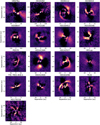 |
Fig. 4 NaCo-ISPY L′ gallery of detected protoplanetary disks. Images have been cropped to highlight the disk morphology and the PSF-subtraction parameters were adapted to show the brightest possible disk residuals. |
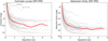 |
Fig. 5 Contrast limits (left) and apparent magnitude detection limits (right) estimated for the ISPY PPD sample as a function of separation. Gray lines represent limits for the individual targets, while the red thick line reports the median limit calculated at each separation. All the curves are obtained for a FPF = 2.87 × 10⁻⁷. |
6.2 The problem of the mass-luminosity conversion
Most of the high-contrast imaging surveys run in the past used age estimates together with evolutionary and atmospheric models to transform flux detection limits into mass upper limits, therefore being able to constrain the planet population potentially detectable by the observations (e.g., Stone et al. 2018; Nielsen et al. 2019; Vigan et al. 2021, to name a few). For forming planets, such an approach strongly relies on several assumptions: (i) atmospheric model, (ii) evolutionary model, (iii) age estimate and age uncertainty, (iv) presence of accretion processes, and (v) extinction along the line of sight. Before proposing an alternative approach in Sect. 6.3, we discuss each of those points with the help of Fig. 6, which shows the magnitude-to-mass conversion for the measured photometries in the H, K and L’ bands of the protoplanet PDS70 b taken from Stolker et al. (2020a) assuming an age of τ = 8 Myr (Wang et al. 2021), with uncertainty σAge = 0 Myr unless stated otherwise.
The choice of atmospheric model used to describe the planet emission might influence the interpretation of the detection limits. For example, different cloud treatments or varying the opacity sources could change the flux in every band. In Fig. 6 the mass estimated from the H-band measurement for the AMES-Dusty (Chabrier et al. 2000) and BT-Settl (Baraffe et al. 2015) model vary by a factor 1.6 (those models assume similar initial entropy following “hot start” scenario). Conversely, the masses estimated from K and L′ photometry seem to be consistent with each other for the two models.
The choice of evolutionary model strongly impacts the emission of substellar objects, especially at young ages (see for example Spiegel & Burrows 2012). In such cases, assuming a hot-, a warm- or cold-start model can strongly bias the final results. Figure 6 shows the mass estimate for hot-start isochrones (AMES-Dusty, BT-Settl) and warm-start models (BEX-warm, Marleau et al. 2019). The warm start models need more massive objects to match the brightness measured for PDS70 b, with a factor ~ 1.7–2.6 difference between the mass values estimated by hot and warm evolutionary tracks.
Age estimates of young stars strongly depend on the method used for the derivation, and different methods very often deliver very different results. Furthermore, depending on the planet formation model, there might be a delay between the time planets and stars start their lives. In Fig. 6 we report the mass uncertainities for σAge = 3 Myr and σAge = 5 Myr as shaded regions (see legend). Especially in the L′-band, the ratio between maximum and minimum mass range is 2.3 (3.2) for σAge = 3 (5) Myr.
Accretion processes from the protoplanet environment onto the circumplanetary disk (CPD) and the planet surface may substantially increase the observed luminosity (e.g., Szulágyi et al. 2014; Zhu 2015; Szulágyi & Mordasini 2017). As a consequence the direct conversion of the measured flux to mass could lead to a biased mass estimate. Finally, extinction from circumstellar (particularly for non face-on disks) and circumplanetary material could influence the emission able to escape the protoplanetary disk, again impacting our ability to convert photometric flux measurements and detection limits into masses (Szulágyi et al. 2018; Sanchis et al. 2020).
From these arguments we can understand that the problem of converting flux measurements into masses is extremely challenging for young forming planets and quickly becomes degenerate. Thus, it is almost impossible to actually constrain the population of forming gas giant planets using the mass as a key population parameter. In particular in the L′-band, the uncertainties related to all these factors suggest that any assessment of the presence of planets and their mass will depend mostly on the underlying assumptions rather than the detection limits estimated from the data.
As an additional consideration, we overplotted in gray the PDS7O b mass estimate obtained when requiring the PDS7O system to be dynamically stable. Most photometric mass estimates seem to disagree with the measured dynamical mass most likely due to one or a combination of the assumptions above. More data are required to validate these preliminary findings and confirm the dynamical mass of PDS70 b, but there is the concrete possibility that at very young ages the standard magnitude to mass conversion is not an appropriate tool to constrain the architecture of infant planetary systems. Similar tensions between dynamical mass measurements and mass estimates based on isochronal fitting were also highlighted in the past. For example, Dupuy et al. (2009, Dupuy et al. 2014) and Kuzuhara et al. (2022) found a relevant difference between the two values for several brown dwarf binaries and companions. In the next Section we try to overcome this problem using existing information on the spectral emission of the forming planets PDS7O b and c.
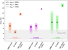 |
Fig. 6 Planetary mass estimate as a function of the assumed evolutionary track, atmospheric model and age uncertainties for the PDS70b protoplanet. Colors represent the different bands considered here and are reported at the bottom of each band. Markers and their error-bars represent the mass estimates when the age is assumed to be known and exact (τ = 8 Myr, σAge = 0 Myr) when using AMES-Dusty (squares), BT-Settl (circles) and BEX-Warm+Cond (diamond). Shaded areas represent the same measurement considering different uncertainties (σAge = 3 Myr for the more intensely colored regions, σAge = 5 Myr for the more transparent regions). The gray region represents the 68% confidence level range of the value for dynamical mass of PDS70b calculated in Wang et al. (2021) thanks to the astrometric precision of the VLTI/GRAVITY instrument. |
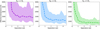 |
Fig. 7 Effective temperature limit of the whole NaCo-ISPY PPD sample assuming Rp = 2RJ (left), Rp = 3RJ (middle) and Rp = 5RJ (right). The dashed line represent the median temperature for the targets having limits extending up to that separations, while the shaded area represents the 16–84% range. |
6.3 Temperatures as a model- and age-independent parameter to constrain the population of forming planets
Pursuing a different approach, we remain as close as possible to the data, obtaining results that are independent from a multitude of arbitrary assumptions. Following recent work on PDS70 b and c, where the SEDs of the planets was found to be well described by a blackbody function (Wang et al. 2020, 2021; Stolker et al. 2020a) and given the lack of detectable molecular features (Cugno et al. 2021), we convert the detection limits into effective temperatures characterizing black body emission. We considered planet sizes of Rp = 2, 3, 5 RJ and we estimated the effective temperature that generates a black body emission bright enough to be detected by our NaCo observations in the L′ filter (the L′ flux was estimated using the NaCo L′ filter transmission profile and the species toolkit, Stolker et al. 2020b).
The three planet radii considered here were chosen based on the following ideas: Ginzburg & Chiang (2019) demonstrated that Rp ≃ 2RJ during the last few Myr of planet formation in case of low opacity (dust-free) atmospheres for a multi-MJ planet, while larger radii (Rp ≈ 5 RJ) can be invoked for young planets whose atmospheres contain considerable amounts of dust. Furthermore, Stolker et al. (2020a) estimated a photometric radius of Rp = 3 RJ for PDS7O b from its SED assuming blackbody emission.
We note that we did not consider smaller planets, for example with Rp = 1 RJ, as this would most likely not be a realistic case for a young multi-MJ planet, as shown by theoretical modeling (e.g., Spiegel & Burrows 2012; Marleau & dimming 2014; Mordasini et al. 2012) and observations of young directly imaged planets so far (Stolker et al. 2020a; Wang et al. 2021; Doelman et al. 2022; Currie et al. 2022). Indeed, during this preliminary phases of their lives, planets are still contracting while emitting a lot of radiation (e.g., Burrows et al. 2001), and therefore they still appear inflated.
In Fig. 7 we show the median and the 16-84 quantiles of the effective temperature limits as a function of the separation from the star. To estimate those limits we considered at each separation only the targets whose images were large enough (see criterion in Sect. 2) and whose disk scattered light emission contaminated the inner part of the images (see Sect. 4.4). As expected, larger planets provide colder limits, while smaller planets could only be detected when hotter. At separations larger than 1″.0, the median temperature limit obtained by our survey is Teff = 1600, 1200, 900 K for Rp = 2, 3, 5 RJ.
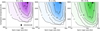 |
Fig. 8 Depth of search for the 45 ISPY-PPD targets included in the analysis, reporting the number of stars to which the survey is complete for young forming planets in the Teff − a parameter space. The three plots represent maps when assuming Rp = 2, 3, 5 RJ (left, middle and right panels, respectively). Overplotted as full black marker the companion HD 101412 B. |
6.4 Survey completeness
To assess the completeness of our survey, we used Monte-Carlo (MC) simulations (Kasper et al. 2007; Nielsen et al. 2008) evaluating the detection probability over a grid uniform in log space in effective temperature (range 600–3000 K, 50 steps) and semi-major axis (range 10–500 au, 50 steps). To each (Teff, a) cell of the grid, 103 planets were assigned with randomly drawn Teff, semi-major axis and orbital phase. The orbital inclination i was assumed to be the same as the disk inclination (see Table A.1). If no inclination has been measured for the disk, sin(i) was randomly drawn with values uniformly distributed between (0,1). Eccentricities are assumed to be e = 0. The other parameters were drawn from uniform distributions. Once planet orbits are simulated, their projected orbital separation is estimated, and if at that separation its effective temperature lies above the 1-D Teff limit curve (Sect. 6.3), they are considered as detected. Conversely, when they lie below the limits, they are considered as nondetectable2. If the projected separation is larger than the image FoV as described in Sect. 2.3 or if the planet is located in the region of the image whose noise is dominated by disk signal and in which no statistically robust limits could have been calculated (Sect. 4.4), we consider the planet as nondetected. The fraction of detected planets for each bin in the Teff − a parameter space provides then an estimate of the fraction of planets potentially detectable around each of our targets.
This procedure provides three detection probability maps for each observed star (one for each assumed Rp). The individual maps were then summed to generate a total completeness map of the survey, shown in Fig. 8 for Rp = 2, 3, 5 RJ. For each combination of semi-major axis and effective temperature, these maps provide the number of stars to which the survey is complete. With a black marker we overplotted in the three maps (independently from its radius) the substellar companion HD 101412 B, the only one in the detection range of our survey. We note that since HD 101412 C is expected to be a stellar companion, its temperature is above the Teff range used in this work. Because of the bright disk ring detected in scattered light (Fig. 4), statistically meaningful detection limits at the separation of PDS70 b and c could not be estimated. Not being in the investigated search space of the survey, the two protoplanets were not included in the main analysis of the demographic of protoplanets, even though in the next Sect. 7.1 we discuss the impact they would have on the results.
7 Discussion
7.1 Occurrence rate of forming planets
We focused on the occurrence rate of forming gas giant planets with temperatures in the range 600–3000 K orbiting with a semi-major axis in the range 20–500 au, as these boundaries reflect the region of parameter space we are interested in and include all the protoplanets known to date. Some past works used population synthesis models to describe the underlying distribution of the planet demographic (e.g., Vigan et al. 2017, 2021), relying on a set of assumptions on the disk and stellar properties as well as on planet dynamical evolution (or the lack thereof). Since little is empirically known about the distribution of forming planets, and many open questions remain on the disk properties, we undertook a simpler approach and assumed that planets are uniformly distributed in semi-major axis and temperature. We then integrate the completeness maps over the range mentioned above, obtaining a completeness to giant planets of 5.5, 7.8 and 10.8 targets for Rp = 2, 3, 5 RJ. Following Nielsen et al. (2019), we considered a Poisson likelihood L and a Jeffreys prior on the rate parameter of a Poisson distribution
 (1)
(1)
where λ is the expected number of planetary systems, that is the frequency multiplied by the completeness of our survey, and k is the number of detected planetary systems (k = 1 in our case). The probability of a given frequency to describe the population of detected planetary systems is plotted in Fig. 9. From this distribution, it follows that the occurrence rate of forming giant planets with the characteristics described above is  ,
,  ,
,  assuming Rp = 2, 3, 5 RJ (68% confidence interval).
Because of the known existence of the PDS70b and c proto-planets (which are located in a disk region excluded in this survey), we also estimated the occurrence rate of forming gas giants assuming two detected planetary systems (k = 2 in Eq. (1)). We found values of  ,
,  and
and  for Rp = 2, 3, 5 RJ. Even though these values are clearly larger than the nominal case presented above, they always fall within 1σ from each other.
The choice of using effective temperatures to describe the planet population contrasts with what is usually done in other high-contrast imaging survey and makes a direct comparison of the detection rates rather difficult. However, if we assume that our temperature range corresponds to the mass range usually considered in high-contrast imaging surveys (e.g., Nielsen et al. 2019; Vigan et al. 2021), our occurrence rates generally agree with their findings: Nielsen et al. (2019) found an occurrence rate of  with a sample of 123 stars with M* > 1.5 M⊙, while Vigan et al. (2021) found occurrence rates of
  and
and  around BA and FGK stars respectively as part of the analysis of the first 150 targets of the SHINE sample.
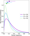 |
Fig. 9 Posterior probability of the frequency of forming systems (20–500 au, 600–3000 K) for the different photometric radii Rp = 2, 3, 5 RJ. Filled circles represent the median of each distribution, while the corresponding errorbars give the 1σ confidence intervals. |
7.2 Sensitivity to distance and extinction from disk material
Figures F.1 and F.2 compare the detection probability maps presented in Fig. 8 with those obtained considering two different cases. First, we limited the considered sample to targets with d < 150 pc (Fig F.1), thus focusing on the nearest 23 targets. The survey completeness for this subsample is almost unchanged. The reason is that for targets at large distance from Earth the innermost region of the protoplanetary disks could not be investigated with NaCo, and at the same time only very hot objects could be detected as the flux scales with 1/d2. Figure F.1 suggests that to constrain planet formation future surveys should focus on the nearby targets, as the innermost region of the disk could be investigated. Here we note the advantage provided by the new class of 30–40 m telescopes, as the spatial resolution will be improved by a factor ~4–5.
Second, we assume that circumstellar disk material absorbs and scatters light emitted by the planet reducing the flux escaping the circumstellar environment by AL′ = 1.0 mag. This is a first order approximation, as different regions of the disk have different dust and gas surface densities and therefore planet flux is affected in very different ways. Furthermore, the presence of gaps and cavities as well as geometrical effects could dramatically change the extinction along the line of sight at different locations. As an example, Sanchis et al. (2020) employed hydrodynamical simulations to estimate the extinction in proto-planetary disks in 8 different bands and found that in the L′-band, a 2 MJ planet opens a relatively small gap and suffers from an extinction of ~1.85 mag at 50 au. To first order, we can expect that in disk regions without gaps the extinction is likely higher, and that in general it decreases with increasing separations as the surface densities drop (especially for the dust), allowing for a decreasing extinction factor. Additionally, more edge-on disks are generally expected to cause stronger attenuation, as the planet flux has to travel through a larger amount of disk material. However, modeling the disk extinction for each of our targets is beyond the scope of this paper, and here we just want to provide a sense of how this aspect may influence results.
The maps for the extinction-corrected case are shown in Fig. F.2, where they are compared to the standard case of Fig. 8. We witness a strong decrease in sensitivity under the assumption that AL′ = 1.0 mag and we are sensitive to objects several hundreds of kelvin hotter than in the nominal case presented in Sect. 6.4. Under the assumption of AL′ = 1.0 mag, the occurrence rates as derived in Sect. 7.1 are  ,
,  and
and  for Rp = 2, 3, 5 RJ (68% confidence interval), highlighting the strong impact of disk attenuation when trying to statistically constrain the population of protoplanets. Including a proper treatment of the dust and gas material in the diskwould most likely increase extinction effects at small separations where pebbles are expected to be present close to the midplane. This would cause the effect of extinction to be even more dominant than in Fig. F.2, strongly impacting the survey completeness. Furthermore, this analysis highlights how detection limits calculated in previous studies might be strongly affected by extincting circumstellar material, especially at short wavelengths (H and K bands, where SPHERE and GPI operate, e.g., Asensio-Torres et al. 2021; Ginski et al. 2022; Mesa et al. 2019b). Indeed, following the extinction law from Mathis (1990), an extinction of 1.0 mag in the L′-band corresponds to AK = 2.0 mag, AH = 3.4 mag and AV = 14.6 mag at shorter wavelengths. Hence, limits from those instruments for protoplanetary disks should be interpreted as lower bounds of our detection capabilities in protoplanetary disks.
Figure F.2 calls for a better characterization of disk extinction properties, and how they may change with disk structures and as a function of the separation from the star and dust grain properties. This is going to be a crucial step in order to properly interpret current and future high-contrast imaging nondetections. In this context, observing in the MIR with upcoming instruments such as JWST/MIRI (Rieke et al. 2015) or the ELT/METIS N-band filter (Quanz et al. 2015b) might overcome the obstacle of the circumstellar material impacting the intrinsic planet flux. For comparison, the extinction expected at 12 µm for the case presented above is A12 µm = 0.5 mag.
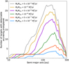 |
Fig. 10 Depth of search for the NaCo-ISPY PPD sample, showing the number of stars to which the survey is complete for accreting objects as a function of |

7.3 Emission from accreting circumplanetary disks
Depending on the system properties, circumplanetary disk emission could be one order of magnitude brighter than the planet’s photospheric emission (Szulágyi et al. 2019). In this section, we investigate the extreme case in which CPD emission dominates the protoplanet radiation, thus constraining ongoing accretion processes. We assumed that the accretion shock is fully thermalized, meaning that its emission can be described once again by a blackbody. Following Gullbring et al. (1998), the accretion luminosity produced can be approximated by
 (2)
(2)
where Rin is the inner truncation radius of the CPD and  is the mass accretion rate onto the planet. The last step assumes that Rin = 5 Rp (e.g., Cugno et al. 2019a). In this section we assume Rp = 3 RJ, but the same reasoning can be applied to the other radii. Once the accretion shock radius has been fixed, Lacc only depends on the
  term, for which we considered different values as reported in Fig. 10. For each
  , we estimated the temperature able to produce a blackbody emission with bolometric luminosity equal to the total accretion luminosity from Eq. (2). We then estimated for how many targets each accretion scenario would have been detected based on the central map of Fig. 8.
Figure 10 clearly indicates that more massive planets and/or objects accreting at a higher rate have a higher chance to be detected. These results suggest that high-mass planets accreting at high rates are rare, especially at separations larger than 100 au, confirming previous searches for accreting protoplanets (Huélamo et al. 2018; Cugno et al. 2019a; Zurlo et al. 2020; Xie et al. 2020).
8 Summary and outlook
We have presented the NaCo-ISPY protoplanetary disk sample, which included observations of 45 young stars with the NaCo instrument at the VLT, searching for forming planets. Observations were carried out in the L′-band and were meant to obtain the highest sensitivity to faint companions. Although the sample size is relatively small compared to other large imaging surveys, which observed hundreds of stars (e.g., GPIES and SHINE, Nielsen et al. 2019; Vigan et al. 2021), the uniqueness of this work lies in the presence of protoplanetary disks surrounding each of the targets. Many of the investigated disks show signposts of ongoing planet formation, such as substructures in the dust and gas distribution likely due to the interaction with embedded forming planets. The PPD sample of the NaCo-ISPY survey offers therefore a unique possibility to probe the population of young forming planets around some of the nearest disks, allowing us to learn important lessons for future surveys.
We detected 15 companions around 13 targets (out of 45), 2 of which with planetary masses (PDS70 b and c), and at least one with estimated mass in the brown dwarf regime (HD 101412 C, see also Rich et al. 2022 and Ruh et al., in prep.).
Disk signals were detected around 17 targets. For two of them, HD 72106 and T CrA, this is the first spatially resolved image of the outer disk.
We showed that the presence of disk signals in the final residuals breaks the assumption of Gaussian noise, therefore strongly biasing results in those regions which should not be trusted.
We highlighted the strong dependence of the mass-to-luminosity conversion for forming planets on the underlying assumptions, showing the difficulties in determining planet masses and how uncertainties dominate every possible result, especially in the L′-band. To overcome these obstacles, we propose a new approach, relying on the study of the SEDs for the forming planets PDS70 b and c.
We estimated the occurrence of forming companions with temperatures in the range 600–3000 K with semi-major axes in the range 20–500 au to be
 ,
,  ,
,  for blackbodies with Rp = 2, 3, 5 RJ respectively.
We show that extinction might be a key factor in the low detection rates, and more advanced calculations of its effect on the flux observed from protoplanets are warranted in order to fully understand and quantify its impact as a function of the separation from the star.
With its MIR capabilities and sensitivity, the James Webb Space Telescope might be able to detect embedded forming companions, increasing the number of directly imaged protoplanets and proving the connection between these objects and the disk features observed with ALMA and high-contrast imagers.
Acknowledgements
We would like to thank the anonymous referee, whose careful and constructive comments improved the quality of this manuscript. G.C. thanks the Swiss National Science Foundation for financial support under grant number P500PT_206785. G.C. and S.P.Q. thank the Swiss National Science Foundation for financial support under grant number 200021_169131. T.D.P. is supported by Deutsche Forschungsgemeinschaft (DFG) grants Kr 2164/14-2 and Kr 2164/15-2. T.H. acknowledges support from the European Research Council under the Horizon 2020 Framework Program via the ERC Advanced Grant Origins 832428. G.M.K. is supported by the Royal Society as a Royal Society University Research Fellow. Part of this work has been carried out within the frame of the National Center for Competence in Research PlanetS supported by the Swiss National Science Foundation (SNSF). S.P.Q. acknowledges the financial support of the SNSF. This work has made use of data from the European Space Agency (ESA) mission Gaia (https://www.cosmos.esa.int/gaia), processed by the Gaia Data Processing and Analysis Consortium (DPAC, https://www.cosmos.esa.int/web/gaia/dpac/consortium). Funding for the DPAC has been provided by national institutions, in particular the institutions participating in the Gaia Multilateral Agreement.
Appendix A Additional tables
Target sample and their main properties used in this work.
Observations of the NaCo-ISPY PPD targets.
Appendix B PSF-subtracted images
Figures B.1, B.2 and B.3 report the residuals obtained after PSF-subtraction for the 45 targets presented in this work. Every scale is shown in au and is based on the target distance and disk extent. The color-scale is linear. Companions and companion candidates are highlighted with a white circle, while the position of indirectly inferred companions which were not detected in our images are shown with dashed white circles. White stars at the center of the images indicate the position of the primary stars.
 |
Fig. B.1 Final PCA-ADI residuals of the ISPY PPD sample. White circles indicate the position of companions. |
 |
Fig. B.2 Final PCA-ADI residuals of the ISPY PPD sample. White solid circles indicate the position of companions, while dashed ones locate background objects. |
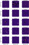 |
Fig. B.3 Final PCA-ADI residuals of the ISPY PPD sample. White solid circles indicate the position of companions, while dashed ones locate background objects. |
Appendix C Noise properties on the residuals
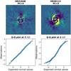 |
Fig. C.1 Noise statistics of the NaCo-ISPY data. Top: Residuals for HD31648 and HD36112 (left and right respectively). The ring highlights the location where the noise is investigated in this figure, at 3λ/D. Bottom: Q-Q plots comparing the noise in the data (blue datapoints) with the expectation from Gaussian noise (gray line). In the right panel the light tails due to the presence of the disk signal and consequent negative self-subtraction cause the noise to deviate from a normal distribution. |
Here we discuss the noise properties of the NaCo-ISPY data, justifying (i) the choice for the underlying noise distribution and (ii) the exclusion from further analysis of regions of the images where bright scattered light disk signals were present. Figure C.1 shows residuals and Q-Q plots for two of our datasets: HD31648 and HD36112. For more information of Q-Q plots we refer to Bonse et al. (2022). The left panel demonstrates that the noise distribution is consistent with Gaussian, even though, as explained in Bonse et al. (2022), we can not undisputedly prove that it is drawn from a Gaussian distribution. In the right panel we show the deviation of the light tails from normal distribution caused by the presence of strong disk signal. Furthermore, in those region the assumption of indipendent noise samples is broken given the correlation induced by the presence of an extended source spread over several resolution elements.
Appendix D Known detected companions
Appendix D.1. HD35187
HD35187 has a known stellar companion and it appears in the Washington Double Star catalog (WDS; Mason et al. 2001) as WDS 05240+2458. According to the catalog, the two stars are separated by 1″.386 ± 0″.005, the PA of the companion is 192° and they have similar brightness (V ≈ 8.5 mag) consistent with our results reported in Table 1. The spectral type of the companion is A7 (Dunkin & Crawford 1998).
Appendix D.2. HD37411
HD37411 is a triple system first identified by Thomas et al. (2007). The ISPY L′ images presented in Fig. B.1 reveal both companions, with their properties reported in Table 1.
Appendix D.3. NX Pup
NX Pup (WDS J07195–4435AB) was revealed to be a binary system with HST images (Bernacca et al. 1993) and was subsequently studied with early adaptive optics systems (Brandner et al. 1995). Our observation is consistent with early detections of the F7-G4 binary companion (Schoeller et al. 1996), and we provide astrometry and L′ photometry in Table 1, obtained with the MCMC algorithm.
Appendix D.4. HD 72106
HD 72106 is a binary system in which the companion is a Herbig Ae/Be star (Vieira et al. 2003). Interestingly, the primary star shows evidence of a strong magnetic field, while the secondary does not (Folsom et al. 2008).
Appendix D.5. HD100453
The companion of HD100453 was first detected by Chen et al. (2006) with the VLT/NaCo instrument. Subsequent HST and NaCo observations confirmed the common proper motion with HD100453 A (Collins et al. 2009) and additional spectroscopic data presented by the same authors constrained the spectral type of the companion to be M4.0-M4.5V. The companion has been observed to move over a short orbital arc (e.g., Wagner et al. 2018), making precise orbital fitting difficult, although dynamical considerations may favour an orbit significantly inclined to the disc (van der Plas et al. 2019; Gonzalez et al. 2020).
Appendix D.6. HD104237
The companion detected in the ISPY data was first imaged by Grady et al. (2004), who resolved the region around HD104237, revealing a small T association (Grady et al. 2005). Furthermore, Grady et al. (2004) demonstrated that a circumstellar disk is surrounding the companion HD104237 B shown in Fig. B.2. The other confirmed companions were at too large separations to be detected.
Appendix D.7. PDS70
PDS70 harbors two forming planets within the large disk cavity (Keppler et al. 2018; Müller et al. 2018; Haffert et al. 2019). Subsequent studies tried to infer several properties from the two companions and their environment (e.g., Wang et al. 2020, 2021; Stolker et al. 2020a; Cugno et al. 2021). The ISPY dataset presented here was first presented in Keppler et al. (2018) and then reanalyzed in Haffert et al. (2019) and Stolker et al. (2020a). For this reason, Table 1 reports the results obtained by Stolker et al. (2020a) for PDS70 b and those from Haffert et al. (2019) for PDS70c.
In addition, in the final residuals a background star north from PDS70 is visible. The nature of the object has already been assessed in Haffert et al. (2019), and therefore we do not investigate it further.
Appendix D.8. HD144432
Initially thought to be a binary system (e.g., Pérez et al. 2004; Carmona et al. 2007), HD144432 was later proven to be triple system, with the B component being actually a close binary itself (Müller et al. 2011). The latter finding was obtained with NaCo imaging data at shorter wavelengths and the spectral classes of the companion binary system (K7 and M1) were inferred using VLT/FEROS spectra (Müller et al. 2011). Our L’ data do not allow us to distinguish the two stars B and C. Thus, we treat it as a single unresolved point source in Table. 1.
Appendix D.9. KK Oph
KK Oph B is a companion known since 1997 (Leinert et al. 1997). Carmona et al. (2007) analyzed VLT/FEROS2 spectra and classified the companion to have spectral type G6.
Appendix D.10. RCrA
The young stellar companion around R CrA was first indirectly inferred by Takami et al. (2003), and then simultaneously imaged with VLT/NaCo (Cugno et al. 2019b) and VLT/SPHERE (Mesa et al. 2019a) observations. The latter authors inferred the spectral type of the object: M3-M3.5. As the data presented here were already analyzed by Cugno et al. (2019b), we report their results in Table. 1.
Appendix E Background objects
Appendix E.1. TYC 7851-810-1
A companion candidate is seen at a separation of 2″.24 from the central star. The object is also resolved in several archival SPHERE observations during 2016 and 2017 presented in Villenave et al. (2019), but without sufficient time baseline and astrometric precision to test for common proper motion.
This object is also resolved in the Gaia catalog, as Gaia DR3 5997490206145064448, at a separation of 2″.306 (Gaia Collaboration 2022). The Gaia catalog does not include parallax or proper motion for this candidate companion, so we instead study the photometry to determine whether the two objects are co-distant. The companion has contrasts of 8.61 ± 0.02 mag and 8.34 ± 0.1 mag in the G and L′ filters respectively. The very similar G − L′ colors of the two objects imply similar spectral types – this is inconsistent with the object being a true companion, given its much lower magnitude.
Appendix E.2. HD 97048
The images of HD 97048 present one companion candidate with a separation of 4″.27 (northwest) from the central star. We reduced archival Gemini/NICI data in the H + K band (Prog. ID:GS-2012A-C-3, PI: Honda) from 2012 in order to determine the proper motion of the companion candidate, which is consistent with a background source.
Appendix E.3. HD163296
Four companion candidates are identified in the residuals of HD163296. All these candidates where already investigated by Mesa et al. (2019b), who verified them and excluded companionship.
Appendix E.4. HD319139
Two companion candidates are identified in the residuals of HD319139. Comparing the images with archival HST images (Prog ID:10348, observation date: 2005-08-03, PI: Herczeg) we could verify that they are all background objects not comoving with the star.
Appendix F Detection probability maps comparison
Here we present the comparison of detection probability maps to low-mass companions when (i) considering only a fraction of the entire sample, namely targets with d < 150 pc, and (ii) when roughly including some extinction from circumstellar disk material potentially attenuating the planetary flux able to escape the circumstellar disk. Case (i) is presented in Fig. F.1, where only the 23 nearest targets are included when generating the survey map. Similarly, case (ii) is shown in Fig. F.2, where we used contrast curves 1.0 mag brighter at each separation due to the extinction from potential circumstellar and circumplanetary disk material.
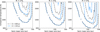 |
Fig. F.1 Detection probability maps obtained from the subsample with d < 150 pc. The three plots represent maps when assuming Rp = 2, 3, 5 RJ (left, middle and right panels, respectively). Solid contours limit the areas with completeness 2, 10 and 20, while dotted lines are reported from Fig. 8 and limit the same completeness values when the entire sample of 45 targets is considered, thus allowing the direct comparison between the two cases and highlighting the dominance of nearby targets when searching for protoplanets and interpreting statistical results. |
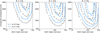 |
Fig. F.2 Survey completeness maps obtained considering an additional extinction factor AL′ = 1.0 mag. The three plots represent maps when assuming Rp = 2, 3, 5 RJ (left, middle and right panels, respectively). Solid contours limit the areas with completeness 2, 10 and 20, while dotted lines are reported from Fig. 8 and limit the same detection probability values when no extinction effects are included, thus allowing the direct comparison between the two cases. |
References
- ALMA Partnership, (Brogan, C. L., et al.) 2015, ApJ, 808, L3 [NASA ADS] [CrossRef] [Google Scholar]
- Amara, A., & Quanz, S. P. 2012, MNRAS, 427, 948 [Google Scholar]
- Andrews, S. M., Wilner, D. J., Hughes, A. M., et al. 2012, ApJ, 744, 162 [NASA ADS] [CrossRef] [Google Scholar]
- Andrews, S. M., Rosenfeld, K. A., Kraus, A. L., & Wilner, D. J. 2013, ApJ, 771, 129 [Google Scholar]
- Andrews, S. M., Huang, J., Pérez, L. M., et al. 2018, ApJ, 869, L41 [NASA ADS] [CrossRef] [Google Scholar]
- Ansdell, M., Williams, J. P., van der Marel, N., et al. 2016, ApJ, 828, 46 [Google Scholar]
- Ansdell, M., Williams, J. P., Trapman, L., et al. 2018, ApJ, 859, 21 [NASA ADS] [CrossRef] [Google Scholar]
- Asensio-Torres, R., Henning, T., Cantalloube, F., et al. 2021, A&A, 652, A101 [NASA ADS] [CrossRef] [EDP Sciences] [Google Scholar]
- Avenhaus, H., Quanz, S. P., Garufi, A., et al. 2018, ApJ, 863, 44 [NASA ADS] [CrossRef] [Google Scholar]
- Bae, J., Zhu, Z., & Hartmann, L. 2016, ApJ, 819, 134 [NASA ADS] [CrossRef] [Google Scholar]
- Bae, J., Pinilla, P., & Birnstiel, T. 2018, ApJ, 864, L26 [Google Scholar]
- Bae, J., Zhu, Z., Baruteau, C., et al. 2019, ApJ, 884, L41 [NASA ADS] [CrossRef] [Google Scholar]
- Balmer, W. O., Follette, K. B., Close, L. M., et al. 2022, AJ, 164, 29 [NASA ADS] [CrossRef] [Google Scholar]
- Baraffe, I., Homeier, D., Allard, F., & Chabrier, G. 2015, A&A, 577, A42 [NASA ADS] [CrossRef] [EDP Sciences] [Google Scholar]
- Benisty, M., Bae, J., Facchini, S., et al. 2021, ApJ, 916, L2 [NASA ADS] [CrossRef] [Google Scholar]
- Bernacca, P. L., Lattanizi, M. G., Bucciarelli, B., et al. 1993, A&A, 278, L47 [NASA ADS] [Google Scholar]
- Beuzit, J. L., Vigan, A., Mouillet, D., et al. 2019, A&A, 631, A155 [NASA ADS] [CrossRef] [EDP Sciences] [Google Scholar]
- Biller, B., Lacour, S., Juhász, A., et al. 2012, ApJ, 753, L38 [Google Scholar]
- Biller, B. A., Males, J., Rodigas, T., et al. 2014, ApJ, 792, L22 [NASA ADS] [CrossRef] [Google Scholar]
- Birnstiel, T., & Andrews, S. M. 2014, ApJ, 780, 153 [Google Scholar]
- Birnstiel, T., Andrews, S. M., Pinilla, R., & Kama, M. 2015, ApJ, 813, L14 [NASA ADS] [CrossRef] [Google Scholar]
- Boehler, Y., Ricci, L., Weaver, E., et al. 2018, ApJ, 853, 162 [Google Scholar]
- Boehler, Y., Weaver, E., Isella, A., et al. 2017, ApJ, 840, 60 [Google Scholar]
- Bohn, A. J., Benisty, M., Perraut, K., et al. 2022, A&A, 658, A183 [NASA ADS] [CrossRef] [EDP Sciences] [Google Scholar]
- Bonse, M. J., Garvin, E. O., & Gebhard, T. D. 2022, ApJ, submitted [Google Scholar]
- Boss, A. P. 1997, Science, 276, 1836 [Google Scholar]
- Brandner, W., Bouvier, J., Grebel, E. K., et al. 1995, A&A, 298, 818 [NASA ADS] [Google Scholar]
- Brandt, T. D., McElwain, M. W., Turner, E. L., et al. 2014, ApJ, 794, 159 [Google Scholar]
- Bruderer, S., van der Marel, N., van Dishoeck, E. F., & van Kempen, T. A. 2014, A&A, 562, A26 [NASA ADS] [CrossRef] [EDP Sciences] [Google Scholar]
- Burrows, A., Hubbard, W. B., Lunine, J. I., & Liebert, J. 2001, Rev. Mod. Phys., 73, 719 [Google Scholar]
- Canovas, H., Hardy, A., Zurlo, A., et al. 2017, A&A, 598, A43 [NASA ADS] [CrossRef] [EDP Sciences] [Google Scholar]
- Cantalloube, F., Gomez-Gonzalez, C., Absil, O., et al. 2020, Proc. SPIE, 11448, 114485A [Google Scholar]
- Carmona, A., van den Ancker, M. E., & Henning, T. 2007, A&A, 464, 687 [NASA ADS] [CrossRef] [EDP Sciences] [Google Scholar]
- Chabrier, G., Baraffe, I., Allard, F., & Hauschildt, P. 2000, ApJ, 542, 464 [Google Scholar]
- Chauvin, G., Lagrange, A. M., Bonavita, M., et al. 2010, A&A, 509, A52 [NASA ADS] [CrossRef] [EDP Sciences] [Google Scholar]
- Chauvin, G., Vigan, A., Bonnefoy, M., et al. 2015, A&A, 573, A127 [NASA ADS] [CrossRef] [EDP Sciences] [Google Scholar]
- Chen, X. P., Henning, T., van Boekel, R., & Grady, C. A. 2006, A&A, 445, 331 [NASA ADS] [CrossRef] [EDP Sciences] [Google Scholar]
- Chen, C. H., Mittal, T., Kuchner, M., et al. 2014, ApJS, 211, 25 [Google Scholar]
- Cleeves, L. I., Öberg, K. I., Wilner, D. J., et al. 2016, ApJ, 832, 110 [Google Scholar]
- Close, L. M., Follette, K. B., Males, J. R., et al. 2014, ApJ, 781, L30 [NASA ADS] [CrossRef] [Google Scholar]
- Collins, K. A., Grady, C. A., Hamaguchi, K., et al. 2009, ApJ, 697, 557 [NASA ADS] [CrossRef] [Google Scholar]
- Cugno, G., Quanz, S. P., Hunziker, S., et al. 2019a, A&A, 622, A156 [NASA ADS] [CrossRef] [EDP Sciences] [Google Scholar]
- Cugno, G., Quanz, S. P., Launhardt, R., et al. 2019b, A&A, 624, A29 [NASA ADS] [CrossRef] [EDP Sciences] [Google Scholar]
- Cugno, G., Patapis, P., Stolker, T., et al. 2021, A&A, 653, A12 [NASA ADS] [CrossRef] [EDP Sciences] [Google Scholar]
- Currie, T., Muto, T., Kudo, T., et al. 2014, ApJ, 796, L30 [Google Scholar]
- Currie, T., Cloutier, R., Brittain, S., et al. 2015, ApJ, 814, L27 [Google Scholar]
- Currie, T., Lawson, K., Schneider, G., et al. 2022, Nat. Astron., 6, 751 [NASA ADS] [CrossRef] [Google Scholar]
- Cutri, R. M., Wright, E. L., Conrow, T., et al. 2013, VizieR Online Data Catalog: II/328 [Google Scholar]
- Di Folco, E., Péricaud, J., Dutrey, A., et al. 2020, A&A, 635, A94 [NASA ADS] [CrossRef] [EDP Sciences] [Google Scholar]
- Dipierro, G., Laibe, G., Price, D. J., & Lodato, G. 2016, MNRAS, 459, L1 [NASA ADS] [CrossRef] [Google Scholar]
- Doelman, D. S., Stone, J. M., Briesemeister, Z. W., et al. 2022, AJ, 163, 217 [NASA ADS] [CrossRef] [Google Scholar]
- Dong, R., Liu, S.-Y., Eisner, J., et al. 2018, ApJ, 860, 124 [NASA ADS] [CrossRef] [Google Scholar]
- Dunkin, S. K., & Crawford, I. A. 1998, MNRAS, 298, 275 [NASA ADS] [CrossRef] [Google Scholar]
- Dupuy, T. J., Liu, M. C., & Ireland, M. J. 2009, ApJ, 692, 729 [NASA ADS] [CrossRef] [Google Scholar]
- Dupuy, T. J., Liu, M. C., & Ireland, M. J. 2014, ApJ, 790, 133 [NASA ADS] [CrossRef] [Google Scholar]
- Facchini, S., Birnstiel, T., Bruderer, S., & van Dishoeck, E. F. 2017, A&A, 605, A16 [NASA ADS] [CrossRef] [EDP Sciences] [Google Scholar]
- Facchini, S., Teague, R., Bae, J., et al. 2021, AJ, 162, 99 [NASA ADS] [CrossRef] [Google Scholar]
- Fairlamb, J. R., Oudmaijer, R. D., Mendigutía, I., Ilee, J. D., & van den Ancker, M. E. 2015, MNRAS, 453, 976 [Google Scholar]
- Fedele, D., Carney, M., Hogerheijde, M. R., et al. 2017, A&A, 600, A72 [NASA ADS] [CrossRef] [EDP Sciences] [Google Scholar]
- Follette, K. B., Rameau, J., Dong, R., et al. 2017, AJ, 153, 264 [Google Scholar]
- Folsom, C. R., Wade, G. A., Kochukhov, O., et al. 2008, MNRAS, 391, 901 [NASA ADS] [CrossRef] [Google Scholar]
- Fung, J., & Dong, R. 2015, ApJ, 815, L21 [NASA ADS] [CrossRef] [Google Scholar]
- Gaia Collaboration 2022, VizieR Online Data Catalog: I/355 [Google Scholar]
- Gaia Collaboration (Arenou, F., et al.) 2023, A&A, in press, https://doi.org/10.1051/0004-6361/202243782 [Google Scholar]
- Garufi, A., Quanz, S. R., Schmid, H. M., et al. 2016, A&A, 588, A8 [NASA ADS] [CrossRef] [EDP Sciences] [Google Scholar]
- Garufi, A., Benisty, M., Pinilla, R., et al. 2018, A&A, 620, A94 [NASA ADS] [CrossRef] [EDP Sciences] [Google Scholar]
- Garufi, A., Podio, L., Bacciotti, F., et al. 2019, A&A, 628, A68 [NASA ADS] [CrossRef] [EDP Sciences] [Google Scholar]
- Garufi, A., Dominik, C., Ginski, C., et al. 2022, A&A, 658, A137 [NASA ADS] [CrossRef] [EDP Sciences] [Google Scholar]
- Ginski, C., Gratton, R., Bohn, A., et al. 2022, A&A, 662, A74 [NASA ADS] [CrossRef] [EDP Sciences] [Google Scholar]
- Ginzburg, S., & Chiang, E. 2019, MNRAS, 490, 4334 [NASA ADS] [CrossRef] [Google Scholar]
- Godoy, N., Olofsson, J., Bayo, A., et al. 2022, A&A, 663, A53 [NASA ADS] [CrossRef] [EDP Sciences] [Google Scholar]
- Gonzalez, J.-F., van der Plas, G., Pinte, C., et al. 2020, MNRAS, 499, 3837 [Google Scholar]
- Grady, C. A., Woodgate, B., Torres, C. A. O., et al. 2004, ApJ, 608, 809 [NASA ADS] [CrossRef] [Google Scholar]
- Grady, C. A., Woodgate, B. E., Bowers, C. W., et al. 2005, ApJ, 630, 958 [NASA ADS] [CrossRef] [Google Scholar]
- Guidi, G., Ruane, G., Williams, J. R., et al. 2018, MNRAS, 479, 1505 [NASA ADS] [CrossRef] [Google Scholar]
- Gullbring, E., Hartmann, L., Briceño, C., & Calvet, N. 1998, ApJ, 492, 323 [Google Scholar]
- Haffert, S. Y., Bohn, A. J., de Boer, J., et al. 2019, Nat. Astron., 3, 749 [Google Scholar]
- Hamidouche, M. 2010, ApJ, 722, 204 [NASA ADS] [CrossRef] [Google Scholar]
- Hammel, B., & Sullivan-Molina, N. 2020, https://doi.org/10.5281/zenodo.3723294 [Google Scholar]
- Huang, J., Andrews, S. M., Dullemond, C. P., et al. 2018, ApJ, 869, L42 [NASA ADS] [CrossRef] [Google Scholar]
- Huélamo, N., Chauvin, G., Schmid, H. M., et al. 2018, A&A, 613, L5 [CrossRef] [EDP Sciences] [Google Scholar]
- Hunziker, S., Quanz, S. P., Amara, A., & Meyer, M. R. 2018, A&A, 611, A23 [NASA ADS] [CrossRef] [EDP Sciences] [Google Scholar]
- Isella, A., Pérez, L. M., & Carpenter, J. M. 2012, ApJ, 747, 136 [NASA ADS] [CrossRef] [Google Scholar]
- Isella, A., Huang, J., Andrews, S. M., et al. 2018, ApJ, 869, L49 [NASA ADS] [CrossRef] [Google Scholar]
- Izquierdo, A. F., Facchini, S., Rosotti, G. P., van Dishoeck, E. F., & Testi, L. 2022, ApJ, 928, 2 [NASA ADS] [CrossRef] [Google Scholar]
- Janson, M., Thalmann, C., Boccaletti, A., et al. 2016, ApJ, 816, L1 [Google Scholar]
- Janson, M., Gratton, R., Rodet, L., et al. 2021, Nature, 600, 231 [NASA ADS] [CrossRef] [Google Scholar]
- Jensen-Clem, R., Mawet, D., Gomez Gonzalez, C. A., et al. 2018, AJ, 155, 19 [Google Scholar]
- Kaltenegger, L. 2017, ARA&A, 55, 433 [NASA ADS] [CrossRef] [Google Scholar]
- Kasper, M., Apai, D., Janson, M., & Brandner, W. 2007, A&A, 472, 321 [NASA ADS] [CrossRef] [EDP Sciences] [Google Scholar]
- Keppler, M., Benisty, M., Müller, A., et al. 2018, A&A, 617, A44 [NASA ADS] [CrossRef] [EDP Sciences] [Google Scholar]
- Keppler, M., Teague, R., Bae, J., et al. 2019, A&A, 625, A118 [NASA ADS] [CrossRef] [EDP Sciences] [Google Scholar]
- Kervella, P., Arenou, F., Mignard, F., & Thévenin, F. 2019, A&A, 623, A72 [NASA ADS] [CrossRef] [EDP Sciences] [Google Scholar]
- Kluska, J., Kraus, S., Davies, C. L., et al. 2018, ApJ, 855, 44 [Google Scholar]
- Konishi, M., Grady, C. A., Schneider, G., et al. 2016, ApJ, 818, L23 [CrossRef] [Google Scholar]
- Kraus, A. L., & Ireland, M. J. 2012, ApJ, 745, 5 [Google Scholar]
- Kurosawa, R., Kreplin, A., Weigelt, G., et al. 2016, MNRAS, 457, 2236 [NASA ADS] [CrossRef] [Google Scholar]
- Kuzuhara, M., Currie, T., Takarada, T., et al. 2022, ApJ, 934, L19 [Google Scholar]
- Lacour, S., Biller, B., Cheetham, A., et al. 2016, A&A, 590, A90 [NASA ADS] [CrossRef] [EDP Sciences] [Google Scholar]
- Lagrange, A. M., Gratadour, D., Chauvin, G., et al. 2009, A&A, 493, L21 [NASA ADS] [CrossRef] [EDP Sciences] [Google Scholar]
- Launhardt, R., Henning, T., Quirrenbach, A., et al. 2020, A&A, 635, A162 [NASA ADS] [CrossRef] [EDP Sciences] [Google Scholar]
- Law, C. J., Loomis, R. A., Teague, R., et al. 2021, ApJS, 257, 3 [NASA ADS] [CrossRef] [Google Scholar]
- Law, C. J., Crystian, S., Teague, R., et al. 2022, ApJ, 932, 114 [NASA ADS] [CrossRef] [Google Scholar]
- Leinert, C., Richichi, A., & Haas, M. 1997, A&A, 318, 472 [NASA ADS] [Google Scholar]
- Lenzen, R., Hartung, M., Brandner, W., et al. 2003, SPIE Conf. Ser., 4841, 944 [Google Scholar]
- Ligi, R., Vigan, A., Gratton, R., et al. 2018, MNRAS, 473, 1774 [Google Scholar]
- Liu, T., Zhang, H., Wu, Y., Qin, S.-L., & Miller, M. 2011, ApJ, 734, 22 [NASA ADS] [CrossRef] [Google Scholar]
- Long, F., Pinilla, P., Herczeg, G. J., et al. 2018, ApJ, 869, 17 [Google Scholar]
- Long, F., Andrews, S. M., Vega, J., et al. 2021, ApJ, 915, 131 [NASA ADS] [CrossRef] [Google Scholar]
- Long, F., Andrews, S. M., Rosotti, G., et al. 2022, ApJ, 931, 6 [NASA ADS] [CrossRef] [Google Scholar]
- Madhusudhan, N. 2019, ARA&A, 57, 617 [NASA ADS] [CrossRef] [Google Scholar]
- Manoj, P., Bhatt, H. C., Maheswar, G., & Muneer, S. 2006, ApJ, 653, 657 [Google Scholar]
- Marleau, G.-D. & Cumming, A. 2014, MNRAS, 437, 1378 [NASA ADS] [CrossRef] [Google Scholar]
- Marleau, G.-D., Coleman, G. A. L., Leleu, A., & Mordasini, C. 2019, A&A, 624, A20 [NASA ADS] [CrossRef] [EDP Sciences] [Google Scholar]
- Marley, M. S., Fortney, J. J., Hubickyj, O., Bodenheimer, P., & Lissauer, J. J. 2007, ApJ, 655, 541 [Google Scholar]
- Marois, C., Lafrenière, D., Doyon, R., Macintosh, B., & Nadeau, D. 2006, ApJ, 641, 556 [Google Scholar]
- Marois, C., Macintosh, B., Barman, T., et al. 2008, Science, 322, 1348 [Google Scholar]
- Marois, C., Zuckerman, B., Konopacky, Q. M., Macintosh, B., & Barman, T. 2010, Nature, 468, 1080 [NASA ADS] [CrossRef] [Google Scholar]
- Martinache, F. 2019, in Imaging at High Angular Resolution of Stellar Surfaces and Close Environment, eds. N. Nardetto, Y. Lebreton, & E. Lagadec (France: EDP sciences), 16 [Google Scholar]
- Mason, B. D., Wycoff, G. L., Hartkopf, W. I., Douglass, G. G., & Worley, C. E. 2001, AJ, 122, 3466 [Google Scholar]
- Mathis, J. S. 1990, ARA&A, 28, 37 [NASA ADS] [CrossRef] [Google Scholar]
- Mawet, D., Absil, O., Delacroix, C., et al. 2013, A&A, 552, L13 [NASA ADS] [CrossRef] [EDP Sciences] [Google Scholar]
- Mawet, D., Milli, J., Wahhaj, Z., et al. 2014, ApJ, 792, 97 [Google Scholar]
- Mawet, D., Choquet, É., Absil, O., et al. 2017, AJ, 153, 44 [NASA ADS] [CrossRef] [Google Scholar]
- Meeus, G., Montesinos, B., Mendigutía, I., et al. 2012, A&A, 544, A78 [NASA ADS] [CrossRef] [EDP Sciences] [Google Scholar]
- Mendigutía, I., Oudmaijer, R. D., Garufi, A., et al. 2017, A&A, 608, A104 [NASA ADS] [CrossRef] [EDP Sciences] [Google Scholar]
- Menu, J., van Boekel, R., Henning, T., et al. 2015, A&A, 581, A107 [NASA ADS] [CrossRef] [EDP Sciences] [Google Scholar]
- Mesa, D., Bonnefoy, M., Gratton, R., et al. 2019a, A&A, 624, A4 [NASA ADS] [CrossRef] [EDP Sciences] [Google Scholar]
- Mesa, D., Langlois, M., Garufi, A., et al. 2019b, MNRAS, 488, 37 [Google Scholar]
- Montesinos, B., Eiroa, C., Mora, A., & Merín, B. 2009, A&A, 495, 901 [NASA ADS] [CrossRef] [EDP Sciences] [Google Scholar]
- Mordasini, C., Alibert, Y., Georgy, C., et al. 2012, A&A, 547, A112 [NASA ADS] [CrossRef] [EDP Sciences] [Google Scholar]
- Müller, A., Carmona, A., van den Ancker, M. E., et al. 2011, A&A, 535, L3 [NASA ADS] [CrossRef] [EDP Sciences] [Google Scholar]
- Müller, A., Keppler, M., Henning, T., et al. 2018, A&A, 617, L2 [Google Scholar]
- Muro-Arena, G. A., Ginski, C., Dominik, C., et al. 2020, A&A, 636, L4 [NASA ADS] [CrossRef] [EDP Sciences] [Google Scholar]
- Musso Barcucci, A., Launhardt, R., Kennedy, G. M., et al. 2019, A&A, 627, A77 [NASA ADS] [CrossRef] [EDP Sciences] [Google Scholar]
- Muto, T., Grady, C. A., Hashimoto, J., et al. 2012, ApJ, 748, L22 [Google Scholar]
- Natta, A., Testi, L., Neri, R., Shepherd, D. S., & Wilner, D. J. 2004, A&A, 416, 179 [NASA ADS] [CrossRef] [EDP Sciences] [Google Scholar]
- Nealon, R., Dipierro, G., Alexander, R., Martin, R. G., & Nixon, C. 2018, MNRAS, 481, 20 [Google Scholar]
- Nielsen, E. L., Close, L. M., Biller, B. A., Masciadri, E., & Lenzen, R. 2008, ApJ, 674, 466 [NASA ADS] [CrossRef] [Google Scholar]
- Nielsen, E. L., De Rosa, R. J., Macintosh, B., et al. 2019, AJ, 158, 13 [Google Scholar]
- Paneque-Carreño, T., Pérez, L. M., Benisty, M., et al. 2021, ApJ, 914, 88 [CrossRef] [Google Scholar]
- Panic, O., Haworth, T. J., Petr-Gotzens, M. G., et al. 2021, MNRAS, 501, 4317 [NASA ADS] [CrossRef] [Google Scholar]
- Pearce, T. D., Wyatt, M. C., & Kennedy, G. M. 2015, MNRAS, 448, 3679 [NASA ADS] [CrossRef] [Google Scholar]
- Pearce, T. D., Launhardt, R., Ostermann, R., et al. 2022, A&A, 659, A135 [NASA ADS] [CrossRef] [EDP Sciences] [Google Scholar]
- Pérez, M. R., van den Ancker, M. E., de Winter, D., & Bopp, B. W. 2004, A&A, 416, 647 [NASA ADS] [CrossRef] [EDP Sciences] [Google Scholar]
- Perryman, M., Hartman, J., Bakos, G. Á., & Lindegren, L. 2014, ApJ, 797, 14 [Google Scholar]
- Pineda, J. E., Quanz, S. P., Meru, F., et al. 2014, ApJ, 788, L34 [Google Scholar]
- Pineda, J. E., Szulágyi, J., Quanz, S. P., et al. 2019, ApJ, 871, 48 [Google Scholar]
- Pinilla, P., de Juan Ovelar, M., Ataiee, S., et al. 2015, A&A, 573, A9 [NASA ADS] [CrossRef] [EDP Sciences] [Google Scholar]
- Pinte, C., Price, D. J., Ménard, F., et al. 2018, ApJ, 860, L13 [Google Scholar]
- Pinte, C., van der Plas, G., Ménard, F., et al. 2019, Nat. Astron., 3, 1109 [NASA ADS] [CrossRef] [Google Scholar]
- Pollack, J. B., Hubickyj, O., Bodenheimer, P., et al. 1996, Icarus, 124, 62 [NASA ADS] [CrossRef] [Google Scholar]
- Quanz, S. P., Amara, A., Meyer, M. R., et al. 2013, ApJ, 766, L1 [Google Scholar]
- Quanz, S. P., Amara, A., Meyer, M. R., et al. 2015a, ApJ, 807, 64 [Google Scholar]
- Quanz, S. P., Crossfield, I., Meyer, M. R., Schmalzl, E., & Held, J. 2015b, Int. J. Astrobiol., 14, 279 [Google Scholar]
- Quiroz, J., Wallack, N. L., Ren, B., et al. 2022, ApJ, 924, L4 [NASA ADS] [CrossRef] [Google Scholar]
- Rameau, J., Chauvin, G., Lagrange, A. M., et al. 2012, A&A, 546, A24 [NASA ADS] [CrossRef] [EDP Sciences] [Google Scholar]
- Rameau, J., Follette, K. B., Pueyo, L., et al. 2017, AJ, 153, 244 [Google Scholar]
- Reggiani, M., Quanz, S. P., Meyer, M. R., et al. 2014, ApJ, 792, L23 [Google Scholar]
- Reggiani, M., Christiaens, V., Absil, O., et al. 2018, A&A, 611, A74 [NASA ADS] [CrossRef] [EDP Sciences] [Google Scholar]
- Ricci, L., Testi, L., Natta, A., & Brooks, K. J. 2010, A&A, 521, A66 [NASA ADS] [CrossRef] [EDP Sciences] [Google Scholar]
- Rich, E. A., Monnier, J. D., Aarnio, A., et al. 2022, AJ, 164, 109 [NASA ADS] [CrossRef] [Google Scholar]
- Rieke, G. H., Wright, G. S., Böker, T., et al. 2015, PASP, 127, 584 [NASA ADS] [CrossRef] [Google Scholar]
- Rousset, G., Lacombe, F., Puget, P., et al. 2003, SPIE Conf. Ser., 4839, 140 [Google Scholar]
- Sallum, S., Follette, K. B., Eisner, J. A., et al. 2015, Nature, 527, 342 [Google Scholar]
- Sanchis, E., Picogna, G., Ercolano, B., Testi, L., & Rosotti, G. 2020, MNRAS, 492, 3440 [Google Scholar]
- Schegerer, A. A., Wolf, S., Hummel, C. A., Quanz, S. P., & Richichi, A. 2009, A&A, 502, 367 [NASA ADS] [CrossRef] [EDP Sciences] [Google Scholar]
- Schoeller, M., Brandner, W., Lehmann, T., Weigelt, G., & Zinnecker, H. 1996, A&A, 315, 445 [NASA ADS] [Google Scholar]
- Skinner, S. L., & Güdel, M. 2020, ApJ, 888, 15 [NASA ADS] [CrossRef] [Google Scholar]
- Soummer, R., Pueyo, L., & Larkin, J. 2012, ApJ, 755, L28 [Google Scholar]
- Spiegel, D. S., & Burrows, A. 2012, ApJ, 745, 174 [Google Scholar]
- Squicciarini, V., Gratton, R., Janson, M., et al. 2022, A&A, 664, A9 [NASA ADS] [CrossRef] [EDP Sciences] [Google Scholar]
- Stapper, L. M., Hogerheijde, M. R., van Dishoeck, E. F., & Mentel, R. 2022, A&A, 658, A112 [NASA ADS] [CrossRef] [EDP Sciences] [Google Scholar]
- Stolker, T., Sitko, M., Lazareff, B., et al. 2017, ApJ, 849, 143 [Google Scholar]
- Stolker, T., Bonse, M. J., Quanz, S. P., et al. 2019, A&A, 621, A59 [NASA ADS] [CrossRef] [EDP Sciences] [Google Scholar]
- Stolker, T., Marleau, G. D., Cugno, G., et al. 2020a, A&A, 644, A13 [EDP Sciences] [Google Scholar]
- Stolker, T., Quanz, S. P., Todorov, K. O., et al. 2020b, A&A, 635, A182 [EDP Sciences] [Google Scholar]
- Stone, J. M., Skemer, A. J., Hinz, P. M., et al. 2018, AJ, 156, 286 [Google Scholar]
- Szulágyi, J., & Mordasini, C. 2017, MNRAS, 465, L64 [CrossRef] [Google Scholar]
- Szulágyi, J., Morbidelli, A., Crida, A., & Masset, F. 2014, ApJ, 782, 65 [CrossRef] [Google Scholar]
- Szulágyi, J., Plas, G. V. D., Meyer, M. R., et al. 2018, MNRAS, 473, 3573 [CrossRef] [Google Scholar]
- Szulágyi, J., Dullemond, C. P., Pohl, A., & Quanz, S. P. 2019, MNRAS, 487, 1248 [Google Scholar]
- Takami, M., Bailey, J., & Chrysostomou, A. 2003, A&A, 397, 675 [NASA ADS] [CrossRef] [EDP Sciences] [Google Scholar]
- Teague, R., Bae, J., Huang, J., & Bergin, E. A. 2019, ApJ, 884, L56 [Google Scholar]
- Teague, R., Bae, J., Aikawa, Y., et al. 2021, ApJS, 257, 18 [NASA ADS] [CrossRef] [Google Scholar]
- Teague, R., Bae, J., Benisty, M., et al. 2022, ApJ, 930, 144 [NASA ADS] [CrossRef] [Google Scholar]
- The, P. S., de Winter, D., & Perez, M. R. 1994, A&AS, 104, 315 [NASA ADS] [Google Scholar]
- Thomas, S. J., van der Bliek, N. S., Rodgers, B., Doppmann, G., & Bouvier, J. 2007, IAU Symp., 240, 250 [NASA ADS] [Google Scholar]
- Trapman, L., Facchini, S., Hogerheijde, M. R., van Dishoeck, E. F., & Bruderer, S. 2019, A&A, 629, A79 [NASA ADS] [CrossRef] [EDP Sciences] [Google Scholar]
- Ubeira Gabellini, M. G., Miotello, A., Facchini, S., et al. 2019, MNRAS, 486, 4638 [NASA ADS] [CrossRef] [Google Scholar]
- Uyama, T., Muto, T., Mawet, D., et al. 2020, AJ, 159, 118 [Google Scholar]
- van Boekel, R., Henning, T., Menu, J., et al. 2017, ApJ, 837, 132 [Google Scholar]
- van der Marel, N., van Dishoeck, E. F., Bruderer, S., Pérez, L., & Isella, A. 2015, A&A, 579, A106 [NASA ADS] [CrossRef] [EDP Sciences] [Google Scholar]
- van der Plas, G., Ménard, F., Canovas, H., et al. 2017, A&A, 607, A55 [NASA ADS] [CrossRef] [EDP Sciences] [Google Scholar]
- van der Plas, G., Ménard, F., Gonzalez, J. F., et al. 2019, A&A, 624, A33 [NASA ADS] [CrossRef] [EDP Sciences] [Google Scholar]
- Verhoeff, A. P., Min, M., Acke, B., et al. 2010, A&A, 516, A48 [NASA ADS] [CrossRef] [EDP Sciences] [Google Scholar]
- Vieira, S. L. A., Corradi, W. J. B., Alencar, S. H. P., et al. 2003, AJ, 126, 2971 [Google Scholar]
- Vigan, A., Bonavita, M., Biller, B., et al. 2017, A&A, 603, A3 [NASA ADS] [CrossRef] [EDP Sciences] [Google Scholar]
- Vigan, A., Fontanive, C., Meyer, M., et al. 2021, A&A, 651, A72 [EDP Sciences] [Google Scholar]
- Villenave, M., Benisty, M., Dent, W. R. F., et al. 2019, A&A, 624, A7 [NASA ADS] [CrossRef] [EDP Sciences] [Google Scholar]
- Vioque, M., Oudmaijer, R. D., Baines, D., Mendigutía, I., & Pérez-Martínez, R. 2018, A&A, 620, A128 [NASA ADS] [CrossRef] [EDP Sciences] [Google Scholar]
- Wagner, K., Dong, R., Sheehan, P., et al. 2018, ApJ, 854, 130 [Google Scholar]
- Wagner, K., Stone, J. M., Spalding, E., et al. 2019, ApJ, 882, 20 [Google Scholar]
- Wang, J. J., Graham, J. R., Dawson, R., et al. 2018, AJ, 156, 192 [Google Scholar]
- Wang, J. J., Ginzburg, S., Ren, B., et al. 2020, AJ, 159, 263 [Google Scholar]
- Wang, J. J., Vigan, A., Lacour, S., et al. 2021, AJ, 161, 148 [Google Scholar]
- Wenger, M., Ochsenbein, F., Egret, D., et al. 2000, A&AS, 143, 9 [NASA ADS] [CrossRef] [EDP Sciences] [Google Scholar]
- Wertz, O., Absil, O., Gómez González, C. A., et al. 2017, A&A, 598, A83 [NASA ADS] [CrossRef] [EDP Sciences] [Google Scholar]
- Winn, J. N., & Fabrycky, D. C. 2015, ARA&A, 53, 409 [Google Scholar]
- Xie, C., Haffert, S. Y., de Boer, J., et al. 2020, A&A, 644, A149 [EDP Sciences] [Google Scholar]
- Zhang, K., Blake, G. A., & Bergin, E. A. 2015, ApJ, 806, L7 [Google Scholar]
- Zhu, Z. 2015, ApJ, 799, 16 [Google Scholar]
- Zhu, Z., Nelson, R. P., Dong, R., Espaillat, C., & Hartmann, L. 2012, ApJ, 755, 6 [Google Scholar]
- Zormpas, A., Birnstiel, T., Rosotti, G. P., & Andrews, S. M. 2022, A&A, 661, A66 [NASA ADS] [CrossRef] [EDP Sciences] [Google Scholar]
- Zurlo, A., Cugno, G., Montesinos, M., et al. 2020, A&A, 633, A119 [NASA ADS] [CrossRef] [EDP Sciences] [Google Scholar]
The bottom left quadrant suffers from bad columns and low sensitivity.
We note that this is a simplification, as contrast curves are not a fixed threshold (Jensen-Clem et al. 2018). However, as we are only interested in the average over the whole survey, this effect is neglected here.
All Tables
Full list of stellar and substellar companions detected in the NaCo-ISPY PPD sample.
All Figures
|
Fig. 1 Stellar and disk parameters for the objects in the ISPY PPD sample. In the top row the histogram for the distances (left) and L′ observed magnitudes (right) are reported. Stellar effective temperatures (left) and masses (right) are shown in the middle row. Finally, the bottom row provides the distributions of the disk outer radius (gas and mm-dust) on the left and disk inclinations (whenever measured) on the right. The dashed vertical lines represent the distance cutoff applied in Sect. 2.4 (top left panel) and the limiting brightness for the coronagraphic observations (top right panel), respectively. |
| In the text | |
|
Fig. 2 Histograms reporting the weather conditions at the time of observations and key parameters describing the datasets. Panel a reports the DIMM seeing, panel b the field rotation, panel c the time spent on each target and panel d the PSF variation, respectively. |
| In the text | |
|
Fig. 3 Proper motion analysis of the stellar companion candidate orbiting HD 38120. The companion motion is inconsistent with a background object, and consistent with being bound. The dark diamond and circle are the 2006 and 2017 positions respectively, the solid line is the expected motion of a background object and the faded diamond is the expected position of a background object in 2017. |
| In the text | |
|
Fig. 4 NaCo-ISPY L′ gallery of detected protoplanetary disks. Images have been cropped to highlight the disk morphology and the PSF-subtraction parameters were adapted to show the brightest possible disk residuals. |
| In the text | |
|
Fig. 5 Contrast limits (left) and apparent magnitude detection limits (right) estimated for the ISPY PPD sample as a function of separation. Gray lines represent limits for the individual targets, while the red thick line reports the median limit calculated at each separation. All the curves are obtained for a FPF = 2.87 × 10⁻⁷. |
| In the text | |
|
Fig. 6 Planetary mass estimate as a function of the assumed evolutionary track, atmospheric model and age uncertainties for the PDS70b protoplanet. Colors represent the different bands considered here and are reported at the bottom of each band. Markers and their error-bars represent the mass estimates when the age is assumed to be known and exact (τ = 8 Myr, σAge = 0 Myr) when using AMES-Dusty (squares), BT-Settl (circles) and BEX-Warm+Cond (diamond). Shaded areas represent the same measurement considering different uncertainties (σAge = 3 Myr for the more intensely colored regions, σAge = 5 Myr for the more transparent regions). The gray region represents the 68% confidence level range of the value for dynamical mass of PDS70b calculated in Wang et al. (2021) thanks to the astrometric precision of the VLTI/GRAVITY instrument. |
| In the text | |
|
Fig. 7 Effective temperature limit of the whole NaCo-ISPY PPD sample assuming Rp = 2RJ (left), Rp = 3RJ (middle) and Rp = 5RJ (right). The dashed line represent the median temperature for the targets having limits extending up to that separations, while the shaded area represents the 16–84% range. |
| In the text | |
|
Fig. 8 Depth of search for the 45 ISPY-PPD targets included in the analysis, reporting the number of stars to which the survey is complete for young forming planets in the Teff − a parameter space. The three plots represent maps when assuming Rp = 2, 3, 5 RJ (left, middle and right panels, respectively). Overplotted as full black marker the companion HD 101412 B. |
| In the text | |
|
Fig. 9 Posterior probability of the frequency of forming systems (20–500 au, 600–3000 K) for the different photometric radii Rp = 2, 3, 5 RJ. Filled circles represent the median of each distribution, while the corresponding errorbars give the 1σ confidence intervals. |
| In the text | |
|
Fig. 10 Depth of search for the NaCo-ISPY PPD sample, showing the number of stars to which the survey is complete for accreting objects as a function of |
| In the text | |
|
Fig. B.1 Final PCA-ADI residuals of the ISPY PPD sample. White circles indicate the position of companions. |
| In the text | |
|
Fig. B.2 Final PCA-ADI residuals of the ISPY PPD sample. White solid circles indicate the position of companions, while dashed ones locate background objects. |
| In the text | |
|
Fig. B.3 Final PCA-ADI residuals of the ISPY PPD sample. White solid circles indicate the position of companions, while dashed ones locate background objects. |
| In the text | |
|
Fig. C.1 Noise statistics of the NaCo-ISPY data. Top: Residuals for HD31648 and HD36112 (left and right respectively). The ring highlights the location where the noise is investigated in this figure, at 3λ/D. Bottom: Q-Q plots comparing the noise in the data (blue datapoints) with the expectation from Gaussian noise (gray line). In the right panel the light tails due to the presence of the disk signal and consequent negative self-subtraction cause the noise to deviate from a normal distribution. |
| In the text | |
|
Fig. F.1 Detection probability maps obtained from the subsample with d < 150 pc. The three plots represent maps when assuming Rp = 2, 3, 5 RJ (left, middle and right panels, respectively). Solid contours limit the areas with completeness 2, 10 and 20, while dotted lines are reported from Fig. 8 and limit the same completeness values when the entire sample of 45 targets is considered, thus allowing the direct comparison between the two cases and highlighting the dominance of nearby targets when searching for protoplanets and interpreting statistical results. |
| In the text | |
|
Fig. F.2 Survey completeness maps obtained considering an additional extinction factor AL′ = 1.0 mag. The three plots represent maps when assuming Rp = 2, 3, 5 RJ (left, middle and right panels, respectively). Solid contours limit the areas with completeness 2, 10 and 20, while dotted lines are reported from Fig. 8 and limit the same detection probability values when no extinction effects are included, thus allowing the direct comparison between the two cases. |
| In the text | |
Current usage metrics show cumulative count of Article Views (full-text article views including HTML views, PDF and ePub downloads, according to the available data) and Abstracts Views on Vision4Press platform.
Data correspond to usage on the plateform after 2015. The current usage metrics is available 48-96 hours after online publication and is updated daily on week days.
Initial download of the metrics may take a while.