| Issue |
A&A
Volume 645, January 2021
|
|
|---|---|---|
| Article Number | A88 | |
| Number of page(s) | 23 | |
| Section | Planets and planetary systems | |
| DOI | https://doi.org/10.1051/0004-6361/202039541 | |
| Published online | 19 January 2021 | |
LIStEN: L′ band Imaging Survey for Exoplanets in the North★
1
Max Planck Institute for Astronomy (MPIA),
Königstuhl 17,
69117 Heidelberg,
Germany
e-mail: This email address is being protected from spambots. You need JavaScript enabled to view it.
2
Department of Physics, University of Warwick,
Gibbet Hill Road,
Coventry CV4 7AL,
UK
3
Landessternwarte, Zentrum für Astronomie der Universität Heidelberg,
Königstuhl 12,
69117 Heidelberg,
Germany
4
Astrophysikalisches Institut und Universitätssternwarte, Friedrich-Schiller-Universität Jena,
Schillergäßchen 2-3,
07745 Jena,
Germany
5
Large Binocular Telescope Observatory,
933 North Cherry Avenue,
Tucson,
AZ 85721,
USA
6
Steward Observatory, Department of Astronomy, University of Arizona,
993 N. Cherry Avenue,
Tucson,
AZ
85721,
USA
7
Department of Physics, University of Notre Dame,
225 Nieuwland Science Hall,
Notre Dame,
IN
46556,
USA
Received:
28
September
2020
Accepted:
18
November
2020
Abstract
Context. Planetary systems and debris discs are natural by-products of the star formation process, and they affect each other. The direct imaging technique allows simultaneous imaging of both a companion and the circumstellar disc it resides in, and is thus a valuable tool to study companion-disc interactions. However, the number of systems in which a companion and a disc have been detected at the same time remains low.
Aims. Our aim is to increase this sample, and to continue detecting and studying the population of giant planets in wide orbits.
Methods. We carry out the L′ band Imaging Survey for Exoplanets in the North (LIStEN), which targeted 28 nearby stars: 24 are known to harbour a debris disc (DD) and the remaining 4 are protoplanetary disc-hosting stars. We aim to detect possible new companions, and study the interactions between the companion and their discs. Angular differential imaging observations were carried out in the L′ band at 3.8 μm using the LMIRCam instrument at the LBT, between October 2017 and April 2019.
Results. No new companions were detected. We combined the derived mass detection limits with information on the disc, and on the proper motion of the host star, to constrain the presence of unseen planetary and low-mass stellar companion around the 24 disc-hosting stars in our survey. We find that 2 have an uncertain DD status and the remaining 22 have disc sizes compatible with self-stirring. Three targets show a proper motion anomaly (PMa) compatible with the presence of an unseen companion.
Conclusions. Our achieved mass limits combined with the PMa analysis for HD 113337 support the presence of a second companion around the star, as suggested in previous RV studies. Our mass limits also help to tighten the constraints on the mass and semi-major axis of the unseen companions around HD 161868 and HD 8907.
Key words: planet-disk interactions / instrumentation: high angular resolution / infrared: planetary systems / techniques: high angular resolution
The LBT is an international collaboration among institutions in the United States, Italy and Germany. LBT Corporation partners are: LBT Beteiligungsgesellschaft, Germany, representing the Max-Planck Society, The Leibniz Institute for Astrophysics Potsdam, and Heidelberg University; the University of Arizona on behalf of the Arizona Board of Regents; Istituto Nazionale di Astrofisica, Italy; The Ohio State University, representing OSU, University of Notre Dame, University of Minnesota and University of Virginia.
© A. Musso Barcucci et al. 2021
 Open Access article, published by EDP Sciences, under the terms of the Creative Commons Attribution License (https://creativecommons.org/licenses/by/4.0), which permits unrestricted use, distribution, and reproduction in any medium, provided the original work is properly cited.
Open Access funding provided by Max Planck Society.
1 Introduction
While the number of detected exoplanets keeps increasing, there are still several missing pieces that are needed to understand the exoplanet population as a whole. Among these the occurrence rate of long-period giant planets (GPs) is still highly uncertain; not only is it governed by the disc structure and planet formation process, but it is also affected by dynamical re-structuring processes after planet formation (like migration and scattering). There is a compelling scientific demand to find and characterise GPs in wide orbits around young stars that cannot be accomplished by the successful indirect detection techniques, like the transit and the radial velocity (RV) technique.
The direct imaging (DI) technique offers a unique opportunity to probe a complementary parameter space with respect to the other indirect exoplanet detection techniques. While the transit and the RV technique are biased towards short-period planets, DI favours companions on wide orbits. The DI technique is capable of detecting objects in a variety of orbital configurations, including face-on orbits, which are not detectable via transits or radial velocity observations. Another advantage lies in the capability of DI to observe very young systems where forming planets might still be embedded in their protoplanetary discs (see e.g. the groundbreaking discovery of PDS 70 b; Keppler et al. 2018). DI also offers the possibility of observing systems where a companion and a circumstellar disc can be imaged and studied simultaneously at the same wavelength, casting light on the intricacies of companion-disc interactions, as in the case of the HR8799 system (Marois et al. 2008), the β Pic system (Lagrange et al. 2010), or the HD 95086 system (Rameau et al. 2013), among others.
The DI technique is therefore an important tool to extend our knowledge of the exoplanet population, and to explore the interaction between companions and the disc they reside in. However, there are several challenges intrinsic to this technique, such as the unfavourable companion-to-star light contrast, the telescope-limited angular resolution and inner working angle (which dictates the minimum separation at which a companion can be detected around its host star), and the long time baseline often needed between follow-up observations to be able to distinguish between physically bound co-moving sources and background objects that might be mistaken for companions. Due to these limitations the number of directly detected companions so far remains scarce (59 confirmed planets with mass ≤ 13 MJup at the time of writing1). Augmentingthis sample is an important scientific goal, and several direct imaging surveys have contributed through the years, targeting different stars and with slightly different scientific goals (see e.g. Bowler 2016). Among others, the Strategic Exploration of Exoplanets and Disks with Subaru (SEEDS; see Tamura 2009; Janson et al. 2013) and more recently a joint high-contrast imaging survey for planets at Keck and VLT (Meshkat et al. 2017) both focused on debris disc-hosting targets in their efforts to find new companions. Janson et al. (2013) surveyed 50 stars using the HiCIAO camera at the Subaru telescope, while Meshkat et al. (2017) used instruments at both the Keck and the Very Large Telescope to target 30 stars with Spitzer-detected debris discs.
The NaCo-ISPY direct imaging survey has just been completed in the southern hemisphere using the NaCo instrument at the VLT telescope in Chile (Launhardt et al. 2020). The survey targets ~200 young and nearby stars with known and well-characterised protoplanetary discs (PPDs) as well as more evolved debris discs (DDs). The ISPY survey aims to increase the number of directly imaged GPs on wide orbits (≥5 au), testing the capability of detecting GPs in the early phases of planet formation (while they are still embedded in their PPDs), and investigating the relation between the DD properties and the presence of wide-separation companions.
In this paper we present LIStEN, the L′ band Imaging Survey for Exoplanets in the North, which has been designed to complement the ISPY survey with observations in the northern hemisphere. The survey was carried out at the Large Binocular Telescope (LBT) on Mount Graham in Arizona between October 2017 and April 2019, using the L/M-band mid-InfraRed Camera (LMIRCam, Skrutskie et al. 2010). The LMIRCam is part of the Large Binocular Telescope Interferometer (LBTI, Hinz et al. 2016), which combines the two apertures of the LBT forsensitive interferometric and imaging observations in the thermal infrared (e.g. Stone et al. 2018; Ertel et al. 2018, 2020) using a cryogenically cooled beam combiner. The standard AO imaging is currently a more routine and stable mode at theLBTI, and it is thus the preferred mode for a large imaging survey such as the one we present. For this reason, for our observations we used the beams from the two apertures separately for high-contrast adaptive optics (AO) assisted direct imaging.
The main goal of the LIStEN survey is to detect and characterise the population of giant planets in wide orbits around young nearby stars with circumstellar discs. For this reason our target selection prioritises stars with known discs (either PPD or DD), inferred either via known infrared excess or resolved images. This target selection also allows us to put the tightest constraints on the planet population, even with non-detections, since the resulting contrast and mass detection limits can be combined with disc knowledge to place constraints on the possible presence of unseen companions. The presence of a companion can influence the morphology and evolution of a debris disc in various and complicated ways. Here we focus on the mechanism known as self-stirring, where large planetesimals grow and stir the disc (see Kenyon & Bromley 2008; Krivov & Booth 2018). An alternative scenario is stirring by secular perturbations from planets or stellar companions (Mustill & Wyatt 2009), but this is most easily explored in systems where the companion is known (see e.g. Musso Barcucci et al. 2019), so we do not consider it here. In cases where discs appear to have multiple temperature components, a common interpretation is that these systems have two distinct disc components (Morales et al. 2011; Kennedy & Wyatt 2014) separated by a gap. Assuming that the gap has been carved out by a planet or planets (as seen in our Solar System and for HR 8799 system), the gap’s parameters can be used to place constraints on the presence of an unseen planetary system (see e.g. Shannon et al. 2016).
In the self-stirring scenario, the evolution of the disc over time is driven by the formation of increasingly large planetesimals that stir their surroundings, triggering destructive encounters and thus generating new dust and material that continuously replenishes the debris disc. The maximum disc size that can be explained via self-stirring at any given time is a function of the host star and disc parameters.
The paper is structured as follows. In Sect. 2 we detail the target selection criteria for the survey, and in Sect. 3 we explain the observational strategy. The data reduction is presented in Sect. 4, together with the data analysis and the creation of contrast curves and mass detection limits. In Sect. 5 we explore the companion-disc interaction and the constraints this can place on the presence of a companion around a given target. Finally, we summarise our results in Sect. 6.
2 Target selection
2.1 Target master list
Our initial source for targets was the Debris Disc Catalogue from the Spitzer Infrared Spectrograph (IRS) observations(Chen et al. 2014). To this we added targets from various sources in the literature, focusing on nearby stars with known and well-characterised discs, both protoplanetary discs and older more evolved debris discs. We excluded targets for which deep angular differential imaging (ADI; Marois et al. 2006) L′ band observations with substantial rotation field (i.e. ≥60°) were already present in the literature in order to minimise the target overlap with other similar surveys2. We also imposed a cut of 200 parsec on the distance. Telescope-specific selection criteria include the following: a cut at Dec ≥−15 degrees in order for the targets to be observable with sufficient field rotation from the LBT location; an R magnitude cut at 13 mag, which is the minimum brightness for high-performance AO corrections; and the exclusion of known close separation (< 1.0″) same-magnitude binaries, which could be difficult for the AO system to distinguish between.
We ended up with a final master target list, from which we had the flexibility of selecting suitable targets depending on the allocated observing nights every semester. During observations, if multiple targets were available, we prioritised nearby targets (in order to probe the ~2−10 au region close to the star) and those targets with a resolved disc (see Sect. 2.2). A total of 28 targets were observed as part of the LIStEN survey during 11 observing nights between October 2017 and April 2019. The observed targets and their basic properties are presented in Table 1. Of these 28 objects, 4 are PPD hosting targets, 22 are surrounded by significant and confirmed DDs, and 2 have a less significant IR excess and an uncertain DD status (HD 184930 and HD 116956). In this paper we present the observations, data reduction, and image inspection for all 28 targets. For the data analysis and the companion-disc interaction analysis we focus on the DD targets only (both the confirmed and the uncertain ones), while the analysis of the four PPD targets will be presented in conjunction with PPD targets observed by the ISPY survey in an upcoming paper.
The target distances are inferred from the Gaia Data Release 2 Catalogue (Gaia Collaboration 2018; Bailer-Jones et al. 2018)and the spectral types are from the Simbad database (Wenger et al. 2000). The ages are compiled from various sources in the literature (see Table 1), which explains the scatter in the age uncertainties for the various targets. An in-depthdiscussion on stellar age determination is beyond the scope of this paper, although we tried to keep our age estimates consistent throughout our survey, and whenever possible relied on age estimates from David & Hillenbrand (2015) and Kains et al. (2011). The stellar masses are taken from Kervella et al. (2019), except when stated otherwise in Table 1. L′ band magnitudes are derived from the ALLWISE data release (Cutri et al. 2013). Starting from the WISE W1 and W2 magnitudes we first computed the colour-corrected fluxes in the two bands (using zero points from Jarrett et al. 2011 and colour-correction factors from Wright et al. 2010); we then obtained the L′ flux as an extrapolation at the L′ wavelength (integrating it over the L′ band filter curve3), and we finally converted this into an L′ band magnitude using the zeropoint provided in Tokunaga (2000).
We show the age, distance, and spectral type distributions for all of our 28 LIStEN targets in Fig. 1. The median distance for our survey is ~49 pc (the closest target being at ~10 pc and the furthest away at ~308 pc4). Given an inner working angle (IWA) of ~ 0′′.150 (see Sect. 3) and the LMIRCam detector plate scale of 10.707 ± 0.012 mas pix −1, we are theoretically sensitive to regions within 10 au from the star for 20 out of our 28 targets. The ages span from 100 to 9700 Myr (with a median age of ~340 Myr) for the DD targets, and from 1 to 9 Myr (with a median of 3.1 Myr) for the PPD targets. Most stars are either A or F type.
LIStEN survey: summary of target parameters.
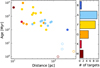 |
Fig. 1 Age, distance, and spectral type distributions for all the LIStEN targets. Distance uncertainties are smaller than the symbol size. Age uncertainties are not shown because they are derived in a non-homogeneous way and are not available for all targets. The stars are colour-coded according to their spectral type. The empty circles are the PPD targets. |
2.2 Notes on individual targets
Out of the 24 DD targets observed during our survey (we do not consider the 4 PPD targets in this section), 14 have a resolved debris disc (at the moment of writing), and 5 have known planetary-mass companions (see Table 1). Even though in some cases these systems are well known, we did not find any available deep L′ band imaging ADI data (with field rotation ≥60°) in the literature, thus making them perfect candidates for our survey. We decided to prioritise these targets, those with a resolved disc and those with known planetary companion(s). We discuss individual cases in the following sections, and summarise the disc and companion information for all of them in Table 2.
2.2.1 HD 206860
HD 206860 (HN Peg, HIP 107350) is a solar-type star at a distance of ~18 parsec. In 2006 Luhman et al. (2007) discovered a substellar companion orbiting the host star at an angular distance of 43″, using the Spitzer Space Telescope. Comparing the luminosity of the object to theoretical evolutionary models, they estimated a mass of ~16 MJup5. Given the large separation of the companion (~790 au), and since our survey focuses on characterising the close-in (≤ 10 au) GP population, we decided to keep this target as part of the LIStEN survey.
2.2.2 HD 183324, HD 191174, and HD 192425
HD 183324, HD 191174, and HD 192425 are early-type stars with double-belt DD, for which Morales et al. (2016) obtained Herschel/PACS imaging data at 70, 100, and 160 μm, with the aim of spatially resolving the outer belt. The dust emission is fit with a thin ring model with three main parameters: radius, inclination, and position angle.
They resolved the colder belt around HD 183324 in all three bands, obtaining a disc radius (at 100 μm) of 2′′. 9±0′′.6, with an inclination of 21° ± 42°. The outer belt around HD 192425 is resolved only at 100 and 160 μm, with a disc size of 4′′. 8±0′′.3 and an inclination of 63° ± 5°. The outer disc around HD 191174 is only partially resolved at 100 μm, yielding a disc size of 3′′. 0±0′′.7 but no constraints on the inclination.
2.2.3 HD 48682, HD 143894, HD 161868, HD 212695, and HD 127821
Five of our targets were imaged with the James Clerk Maxwell Telescope (JCMT) as part of the SONS survey of debris discs (Holland et al. 2017). They obtained sub-millimetre images at 850 and 450 μm and, via radial profile fitting, derived radial extent, inclination, and position angle for all the sources with a resolved emission, while providing disc size upper limits for the unresolved ones.
The discs around HD 48682, HD 143894, and HD 161868 were all resolved at 850 μm, with an estimated disc size of 11′′. 0±3′′.9, 10′′. 2±2′′.5, and 7′′. 8±2′′.2, respectively. They derive a disc inclination of 67° ± 24° for HD 143894, and provide a lower limit of 47° on the disc inclination for HD 48682 and 16° for the disc around HD 161868.
The discs around HD 212695 and HD 127821 were unresolved, yielding a disc upper limit of 7′′. 5 and 7′′. 4, respectively.
2.2.4 HD 110897
HD 110897 is a solar-type star at a distance of ~17.5 parsec. Herschel/PACS observations were obtained as part of the DUNES and DEBRIS surveys, with the aim of resolving and characterising its circumstellar disc (Marshall et al. 2014). Extended emission from the disc is resolved in the 70, 100, and 160 μm bands, and the best-fit model is a cool broad dust ring with a peak in the surface brightness at ~ 3′′. 1 (~50 au) and an inclination of 56° ± 10°. Our survey is therefore able to explore the region within the disc and could potentially detect brown dwarf companions (smaller objects would be harder to detect due to the somewhat old age of the system), making this target a perfect candidate for LIStEN.
2.2.5 HD 50554
HD 50554 is an F8-type star at a distance of ~31 parsec, with a known planetary-mass companion discovered with the RV technique by the ELODIE survey (Perrier et al. 2003). The companion has an estimated mass of mp sini = 5.16 MJup and a semi-major axis of 2.41 au.
Herschel/PACS observations at 70, 100, and 160 μm revealed extended emission around the host star (Dodson-Robinson et al. 2016), whose best fit yields a disc size of 1′′. 45±0′′.13 (45 ± 4 au). The LIStEN survey is designed to explore regions down to ~10 au around its targets, and this star is therefore a very interesting candidate that would allow us to explore the gap between the known planetary companion at a few au and the disc, further away at a few tens of au. Given the system age, we expect to be able to detect any brown dwarf companion in this region.
LIStEN survey: summary of resolved discs and hosted planets.
2.2.6 HD 8907
HD 8907 was observed with the Submillimeter Array (SMA) and Combined Array for Research in Millimeter-wave Astronomy (CARMA) by Steele et al. (2016), resolving its debris disc for the first time. The best fit of its spectral energy distribution (SED) and resolved images yields a disc size of 1′′. 59±0′′.76 with an inclination of 65°. HD 8907 was also observed by Holland et al. (2017) during the SONS survey; they obtain an upper limit on the disc radius of 5′′. 1, in agreement with the results of Steele et al. (2016).
2.2.7 HIP 83043
HIP 83043 (GJ 649, BD+25 3173) is a nearby (~10 parsec) M-type star, which was observed with Herschel/PACS at 100 and 160 μm by Kennedy et al. (2018). They partially resolve the disc at 100 μm, and conclude that the emission is consistent with an edge-on disc with an extent between ~ 1′′.0 and ~ 2′′.9 (between 10 and 30 au).
The host star is also known to harbour a close-in companion, discovered with the RV technique by Johnson et al. (2010), with an estimated mass of mp sini = 0.328 MJup. At a distance of ~1.1 au, the companion resides well within the disc.
This target is an excellent candidate for the LIStEN survey since its distance and our IWA of ~ 0′′.150 (see Sect. 3) mean that we would be able to probe the gap between the known RV planet and the resolved circumstellar disc.
2.2.8 HD 128311
HD 128311 (HIP 71395, GJ 3860) is a K-type star at a distance of ~16 parsec, hosting two close-in planetary-mass companions discovered with the RV method: HD 128311 b, with an estimated mass of mp sini = 2.18 MJup and a semi-major axis of ~1 au, and HD 128311 c with a mass of 4.19 MJup and semi-major axis of 1.76 au (Butler et al. 2003; Vogt et al. 2005). The star is also known to harbour a circumstellar disc with a radius of 58 au6. The LIStEN survey is therefore perfectly designed to probe the region between the two known RV planets and the debris disc, allowing us to gain more information on this interesting system.
2.2.9 HD 113337
HD 113337 is an F6 main-sequence star at a distance of ~36 parsec, known to harbour a debris disc due to its infrared excess; it has at least one confirmed giant planet with a minimum mass of 3.1 MJup at ~1 au and one companion candidate with a minimum mass of 7.2 MJup at ~5 au, detected with the RV technique (Borgniet et al. 2014, 2019b).
Borgniet et al. (2019a) carried out an extensive study of this system, partially resolving its debris disc for the first time at 70 and 160 μm with Herschel/PACS, and obtaining ADI L′-band data using the LMIRCam at LBT. They derived a disc size of 85 ± 20 au with an extension of 30 ± 20 au, and an inclination of 10−30°. Combining RV data, imaging contrast limits, and age and inclination solutions, they derive an estimate for the true masses of the two companions of  for the confirmed companion HD 113337 b, and
  for the candidate companion HD 113337 c.
We observed HD 113337 in the context of the LIStEN survey prior to the publication of the study from Borgniet et al. (2019a). Furthermore, the L′ band ADI observations presented in Borgniet et al. (2019a) were obtained in January 2015, and thus our additional imaging data would allow us to span a baseline of more than 4 yr. For these reasons we decided to keep HD 113337 in our target list and to analyse it independently of the results of Borgniet et al. (2019a), while keeping them in mind as a useful benchmark.
3 Observations
Observations were carried out using the LMIRCam instrument (Skrutskie et al. 2010) at the LBT in Arizona with the L′ -band filter at 3.8 μm, during 11 nights between October 2017 and April 2019. All the observations were carried out in visitor mode, with the exception of the observation in February and April 2019.
Our observational strategy makes simultaneous use of the two 8.4-m mirrors of the LBT, and consists of L′ band ADI observations in non-overlapping dual mode, bracketed with unsaturated flux measurements in order to create an unsaturated point spread function (PSF) reference for each mirror. The dual mode allows us to keep the light coming from the two mirrors separated on the detector, thus creating two images of the same star, allowing for two simultaneous and semi-independent observations of a given target.
During observations we positioned the star images on the left side of the detector at a distance of ~ 5′′. 0 from each other (to avoid cross-contamination between the two PSFs) and collected data with a left-right nodding pattern with a typical frequency of 150 frames per side (10 frames per side for the unsaturated flux measurements). The exposure time for the science frames, typically around ~1 s, was chosen in order to maximise the sensitivity for each target while avoiding the stellar PSF saturating beyond ~ 0′′.100-0′′.150. Given the average distance between the star images (from the two mirrors), and to avoid cross-contamination between the two PSFs, our observational set-up allows us to probe the region around a given target between ~ 0′′.150 and ~ 2′′.0. The exposure time for the flux measurements was chosen to avoid saturation of the PSF, and for certain targets we had to use a 10% neutral density filter. Our aim was to observe each target for a minimum of 2 h around its meridian passage to achieve a total field rotation of ≥ 60 degrees.
We adopted this same observational strategy for all the LIStEN targets as much as possible, however we had to carry single-sided observations for some of our targets due to technical issues with either of the two AO systems. The observing dates for all of our DD targets, together with flux and science detector integration time (DIT), information on single or dual mode observations, and total field rotation, are reported in Table 3.
4 Data reduction and analysis
4.1 Dataprocessing
All data are reduced with our own reduction pipeline, which has been tailored to the specific observational strategy we adopted. The creation of the master flats and the bad pixel maps is detailed in Appendix A. The pipeline is fully automated, except for a few initial target-dependent parameters that need to be input manually. The type and purpose of these parameters, and a full description of the data reduction pipeline is detailed as follows:
Data organisation
The frames are separated into unsaturated flux frames and saturated science frames depending on their DITs, and all the frames with the “bad frame” tag in the header are removed. This tag is automatically created during the observations for those frames that clearly exhibit bad behaviour (i.e. when an incorrect offset is applied to the target the entire frame is almost completely saturated) and similar extreme cases. The following analysis was performed separately on both the flux and the science frames.
Locatingthe star position(s)
According to the target-dependent bad pixel map (see Appendix A), the bad pixels are masked and then the image is smoothed out using the ndimage.gaussian_filter of the scipy Python package, with sigma = 2 pixels. The rough position of the star(stars) is finally found as the position of the absolute maximum(maxima), above a manually set threshold, in this masked smoothed frame. Only frames in which the correct target-dependent number of stars is found are then used (either one or two stars, whether a single- or double-dish observation).
Nod separation
The frames are divided into the two nod positions (nodA and nodB), according to the position of the star(s) in each frame and the target-dependent pixel separation between the nods.
Sky subtraction
A master sky is created from each nod with a principal component analysis (PCA) approach. Each frame in a given nod is sky-subtracted using the master sky created with the other nod, and flat-fielded using the target-dependent master flat (depending on the observing run). During this step the bad pixels are masked according to the target-dependent bad pixel map. The frame is then cut into two, separating the DX and SX mirror (only for dual-mirror observations), and each sub-frame is saved separately. From this point on the frames for different mirrors are reduced separately and independently from each other.
Bad pixel correction
The bad pixels are now corrected for by interpolating from the neighbouring pixels with a Gaussian kernel with standard deviation of 2 pixels.
Bad stripes correction
The pixel-corrected frames are padded with zero to regain the initial target-dependent window size. In each frame, the median of all the pixel values throughout the entire datacube (for a given pixel) is subtracted from that pixel to correct for bad stripes and similar effects. To avoid contamination from the star and possible contamination from the other mirror’s star at the edge of the frame, the median evaluation is done on a datacube in which a square of size 100×100 pixels around the position of the star is blanked out; a frame of 120 pixels in width all around the edges of the frame is also blanked out. These final padded and median-subtracted frames are saved.
De-warping
Every frame is now corrected for the distortions introduced by internal LBT optics, and by the fact that the pixels on the CCD detector are not in a perfect cartesian grid. The distortion correction coefficients for a given semester are available on the LBTO wepage7. Since these corrections have been evaluated for the entire detector array of 2048×2048 pixels, the frames are accordingly padded with zeros before being de-warped. The de-warped frames are then cut down again to their target-dependent window size before being saved.
LIStEN survey: summary of observations.
Centring
The position of the star on these de-warped frames is re-evaluated as the position of the maximum pixel value, and the frame is cut in a square shape around this position with a fixed stamp size of 400 × 400 pixels. A finer sub-pixel centring is then performed finding the 2D Gaussian centroid of each frame. The final centred frames are then saved in their respective mirror folder.
Stacking
This step was performed only for the science frames. Frames with less than 0.1 deg change in the parallactic angles are stacked together (i.e. mean combined) to reduce the total number of frames. This is helpful in the subsequent data analysis to maintain manageable computational times for each target. This stacking does not influence significantly the achievabledetection limits and it seems, for certain targets, to even improve them (see Appendix B).
For the rest of the analysis we use these reduced stacked science frames, keeping the analysis of the two mirrors separated and independentfrom each other.
The reduced flux frames are median-combined (for each mirror) to create one single reduced flux frame per mirror (for each target). These flux frames are then scaled according to the DITs of the science frames and used to create and inject fake negative planets during the creation of contrast curves (see Sect. 4.3).
4.2 PynPoint analysis
The reduced data was analysed using the PynPoint package (Amara & Quanz 2012; Stolker et al. 2019), which uses a PCA-based approach to model and subtract the central PSF, where the main parameter is the number of principal components (PCs) used. We refer to these papers for a detailed explanation on the functionality of the package and its various modules.
We resized the frames to stamps of size 4′′.2 × 4′′. 2, and we used a central mask of 0′′.1 to block the light from the central star (corresponding to the area within which the pixels were saturated during observations). We then analysed the data with a range of values: PC from 1 to 100, plus PC as a fixed fraction, 1, 2, 5, 10, 20, 30 and 50%, of the total number of frames. The images are corrected for the true north offset for LMIRCam of − 0.430° ± 0.076° (Maire et al. 2015).
All the reduced images were inspected by eye, making use of the simultaneous and semi-independent observations with the two mirrors (when applicable) to distinguish between real companion candidates and persistent speckles. An example of the final PCA-reduced image for one of the targets is shown in Fig. 2 for a representative PC number of 20, for both mirrors. A close-in companion-like feature is visible north of the star in the DX mirror image, and its position is indicated with a black arrow in both mirrors; however, comparison with the SX mirror image of the same target reveals no such feature at the same location, thus suggesting that it is a non-physical object, likely a bright speckle.
The final PCA-reduced images for all the 28 targets and both mirrors (where applicable) are shown in Figs. A.6–A.8, for a representative PC number of 20. All the images were inspected by eye and no new companion candidates were detected. One of the PPD targets, HD 35187, has a known stellar companion which we re-detected (bright spot in the bottom right corner of the image, see corresponding panel in Fig. A.6). Four of our targets have confirmed planetary companions detected with the RV method, with masses between ~ 0.3 and ~ 16 MJup. However, these objects are too close to their host stars to be detected in our DI survey, with most of them having an angular separations of ≤ 0′′.10. The most DI-favourable companion would be the candidate around HD 113337, at an angular separation of ~ 0′′.13, but its mass of ~16 MJup is below our achieved detection limits for this target (see Table A.1). One of our targets, HD 206860, has a companion detected via direct imaging, but its large angular separation of ~ 44′′.0 falls outside the field of view for our observations. HD 36112 (MWC758) has a known and well-studied disc (see e.g. Reggiani et al. 2018); while an in-depth analysis of the disc image is beyond the scope of this paper, we note that we nicely recover the spirals in our PCA-reduced image (see Fig. 3), which serves as proof of concept for the validity of our reduction.
For the rest of the paper we focus only on the DD targets, whether with confirmed or uncertain status, and we defer the analysis of the PPD targets to an upcoming paper.
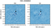 |
Fig. 2 ADI reduced images of HD 206860 for both mirrors, for a representative PC number of 20. The images are oriented with north up and east left, and the colour map has been chosen to better visualise the data. The black arrow gives the position of a suspicious feature in the DX image, ruled out as a speckle thanks to the comparison with the SX image. |
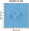 |
Fig. 3 ADI reduced image of HD 36112 (DX mirror only). The disc spirals are clearly visible. |
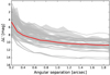 |
Fig. 4 Contrast curves (5 σ) for all targets, and both mirrors where applicable (grey lines). The grey shaded area around each curve represents the 1 σ uncertainty range. The thick red line shows the median of all contrast curves. |
4.3 Contrast curves and mass limits
We evaluated the contrast limits at various separations for each target and for each mirror using the dedicated contrast curve module in PynPoint. This package uses the unsaturated PSF of the central star to create and inject fake negative planets with varying magnitude contrast at the desired separations and azimuthal angles, and creates contrast curves given the desired sigma level and/orfalse positive fraction (FPF), corrected for small sample statistics according to Mawet et al. (2014). The package allows us to account for the possible presence of a neutral density filter, which is the case for some of our targets (see Table 3). The other main free parameter is the aperture radius, which we fixed at 1 FWHM (~ 0′′.116).
The contrast curves are sampled between 0′′.2 and 1′′. 9 in steps of 0′′. 1, and between 0° and 360° in steps of 45°, with thresholds of 1, 2, 3, and 5σ. The resulting 5σ contrast curves for all the targets (and for both mirrors, if applicable) are shown in Fig. 4, where the grey shaded area represents the uncertainty on the magnitude contrast derived as variance of the all the contrasts at various azimuthal angles for a given separation. We achieve a median contrast of ~ 4.5 mag at an angular separation of 0′′.2 from the host star, while far away we are limited by the median background limit and we reach ~ 10.7 mag at ~ 2′′.0. The achieved contrast for all the DD-hosting targets are reported in Table A.1. If a target was observed with both mirrors, we only list the values derived from the better performing mirror.
We convert the contrast curves into mass detection limits as follows. Using the uncertainty ranges for the L′ -band magnitude, contrast, distance, and age for each target (see Table 1), we draw with Gaussian priors from these uncertainties 1000 samples, derive the mass detection limit for every sample at every radial point using the AMES-COND evolutionary models (Allard et al. 20128), determine the median (50% quantile) as the expectation value, and determine the 25 and 75% quantiles as lower and upper bounds. If no age uncertainty is available, we arbitrarily set it to 50% of the age. The achieved mass limits (in MJup) for all the DD targets as a function of the distance from the host star (in au) are shown in Fig. A.3 for both mirrors (DX mirror in blue and SX mirror in green). We also show the position of the disc (either inferred via SED in black, or resolved in red), both for single- and double-belt systems. If a belt is not visible in the field of view, we mark its position with a black (SED-inferred) or red (resolved) arrow.
We then used these mass detection limits to evaluate the detection space for our survey with an approach similar to that in Launhardt et al. (2020): we run Monte Carlo (MC) simulations in which we assign a companion to each target, randomising its mass, semi-major axis, orbit inclination, and orbital phase. The semi-major axis and mass are drawn from log uniform probability distributions with boundaries of [100.05, 103.25] au and [10−1.05, 102.05] MJup. The eccentricity is set to zero, and the inclination is drawn so that all disc orientations in a 3D space are equally probable. For those planets for which we have information about the inclination of the disc (see Table 2), we assume co-planarity for the simulated companions and we draw the inclination given the known constraints.
For each simulated planet we then verify if it would have been detected by our survey, given our achieved mass limits. We generated 107 simulated planets per star, and estimated the error as the standard error on the weighted mean of 100 sets of 105 companions. The resulting detection probability map is shown in Fig. 5. We achieved a detection probability of greater than 50% for companions more massive than ~30 MJup between ~30 and ~100 au.
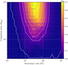 |
Fig. 5 Survey detection probability as a function of companion mass and true (not projected) semi-major axis. |
4.4 Infrared excess characterisation
All of our targets were pre-selected based on their infrared excess, which normally indicates the presence of a debris disc. To better constrain the target parameters such as stellar luminosity and effective temperature, as well as debris disc dust temperature, fractional luminosity, and black-body (BB) radius, we fit the SED for each target.
We simultaneously fit a stellar atmosphere (PHOENIX; Husser et al. 2013) plus a single or double BB model to the observed photometry and the Spitzer IRS spectrum (here obtained from the CASSIS database; see Lebouteiller et al. 2011). The photometry is compiled from various archives and covers a wide range of filters and wavelengths, including: “Heritage” Stromgren and UBV (Paunzen 2015), 2MASS (Skrutskie et al. 2006), HIPPARCOS/Tycho-2 (ESA 1997, The hipparcos and Tycho Catalogues, ESA SP-1200, ESA 1997), AKARI (Ishihara et al. 2010), WISE (Wright et al. 2010), and Spitzer (Chen et al. 2014). The fitting method finds the best-fit model with the MultiNest code (Feroz et al. 2009), using synthetic photometry of grids of models. An exampleof such a fit is shown in Fig. 6 (see Yelverton et al. 2019 for further details on the method).
For 18 of our targets, the best fit is obtained with a stellar model plus a one-temperature BB model. Four targets are better fit with two BB components, which are thought to arise from two belts with two temperatures, one for the outer cold belt and one for an additional inner warm belt. For two targets the infrared excess turned out to be not significant and their SEDs can be simply modelled with only the stellar model. The SED fits for all 24 targets are shown in Fig. A.2. We point out that a single-belt fit does not exclude the presence of a second temperature component since the data availability, quality, and wavelength coverage strongly affects the sensitivity for detecting a component at all.
The BB radius of the dust disc is given by Pawellek & Krivov (2015):
 (1)
(1)
An estimate of the “true” disc radius, Rdisc, can be obtained applying a stellar luminosity-dependent correction factor, Γ, which accounts for the fact that small grains that dominate the emission are typically overheated as they are inefficient in emitting at infrared wavelengths (Pawellek & Krivov 2015):
 (2)
(2)
Throughout this paper we use the new coefficients derived by Pawellek (2016): a = 7.0 and b = −0.39.
With this correction, we estimate true disc sizes for the cold belts of all of our targets. This correction cannot be applied to the warm belt, since the underlying grain properties for those temperatures is unconstrained due to the lack of well-resolved observations of warm belts. The stellar and disc parameters (radii corrected for blowout grain size) for all of our DD targets are summarised in Table 4.
 |
Fig. 6 Flux density distribution of HD 50554. The blue points are the photometric datapoints found in the literature, the black line is the IRS spectrum, and the green and red lines are the fitted stellar and disc fluxes, respectively. |
Disc parameters from SED fitting.
5 Planetary constraints and disc analysis
In this section we derive constraints on the presence of companions around the 22 targets with a confirmed debris disc, using the mass detection limits derived in Sect. 4.3, the disc information, and the constraints from the proper motion of the host star.
5.1 Self-stirring analysis
Of the 22 confirmed targets that host a debris disc in our survey, 18 are well explained with a single-belt model and 4 require an additional component (i.e. the double-belt model is preferred). All the double-belt systems and 10 out of the 18 single-belt systems alsohave a resolved disc size.
We can test the hypothesis that these systems are completely self-stirred, and thus they do not require the presence of a planet to explain the presence of collisionally generated dust at the observed radii. Following the work from Krivov & Booth (2018), the self-stirring timescale can be expressed as a function of the disc’s and host star’s parameters as
![Mathematical equation: \begin{equation*}\begin{split} \hspace*{-2pt}T_{\mathrm{stir}}= & \frac{129\,\mathrm{Myr}}{x_{\mathrm{m}}}\times\left(\frac{1}{\gamma}\right)\,\left(\frac{\rho}{\mathrm{1\,g\,cm^{-3}}} \right)^{-1}\,\left(\frac{v_{\mathrm{frag}}}{\mathrm{30\,m\,s^{-1}}}\right)^{4}\,\\[4pt] \hspace*{-2pt}& \times\left(\frac{S_{\mathrm{max}}}{\mathrm{200\,km}}\right)^{-3}\times\left(\frac{M_{\star}}{{M}_{\odot}}\right)^{-3/2}\,\left(\frac{a}{\mathrm{100\,au}}\right) \end{split}; \end{equation*}](/articles/aa/full_html/2021/01/aa39541-20/aa39541-20-eq5.png) (3)
(3)
here xm is a dimensionless parameter proportional to the disc’s mass, γ has a value between 1 and 2 and encapsulates the eccentricity behaviour of the planetesimals, ρ is the bulk density of the planetesimals and Smax their maximum size, and vfrag is the relative fragmentation velocity above which planetesimals would undergo destructive collisions and thus ignite a collisional cascade through the disc.
We can now compare Tstir with the age of the observed systems as a function of disc radius (a), for a given stellar mass M⋆. We fixed the following parameters to the standard values used in Krivov & Booth (2018): γ = 1.5, ρ = 1 g cm-3, vfrag = 30 ms-1, and Smax = 200 km. The results for all the single-belt systems in our survey are shown in Fig. A.4, where the shaded blue area encompasses two representative values for xm of 1 (dashed line) and 10 (full line). For the double-belt systems, we test the self-stirring assumption on the outer belt only, and the results are shown in Fig. A.5.
Kenyon & Bromley (2008) originally found consistently longer stirring timescales for a slightly different self-stirring scenario, deriving an analytical formula for the stirring timescale:
 (4)
(4)
For comparison, we show the analysis from Kenyon & Bromley (2008) as a red shaded area in Figs. A.4 and A.5, again for representative xm values of 1 (dashed line) and 10 (full line).
The main difference between the two studies is the initial size of planetesimals after the dispersal of the protoplanetary discs. Kenyon & Bromley (2008) assume that planetesimals are born with sizes below 1 km, and find that only by the time these planetesimals grow to Pluto-sized bodies (~ 1000 km), they are able to quickly self-stir the disc. Krivov & Booth (2018) instead argue that bodies as small as ~ 200 km can already excite planetsimals to the point of destructive collisions.
In Figs. A.4 and A.5 we also plot the ages and disc sizes for all of our targets, both SED-derived (in black) and resolved disc sizes (in red). As can be seen for all of our targets, the disc size is smaller than the maximum disc size explainable with self-stirring only, thus confirming that all of these systems can be explained via self-stirring. We note that this does not exclude that planetary-stirring is in action, nor does it exclude the presence of unseen planets, but it merely implies that a companion is not necessary to explain the observed disc sizes. Moreover, the estimated self-stirring timescale using Eq. (3) relies on poorly constrained parameters such as the maximum planetesimal size, thus this conclusion could depend on the parameters chosen. We also note that these results rely on accurate age and disc size measurements, and any future improvement in this regard might help to confirm (or deny) the self-stirring hypothesis, and guide future observations.
5.2 Double-belt analysis
Four of our targets are double-belt systems, for which the colder and outer belt has been resolved through imaging (see Table 2). One explanation for the presence of a wide gap between two belts is the carving action of one or more planets clearing its orbit, and the radius and width of this gap can therefore be related to the minimum planetary mass and minimum number of planets of that given mass required to carve such a gap (see Fig. 1 in Shannon et al. 2016).
Shannon et al. (2016) carried out such an analysis employing N-body simulations to study the clearing times for various planetary systems, assuming coplanar planets on circular orbits each separated by 20 mutual Hill radii (according to similar results obtained by Fang & Margot 2013). They assigned the debris disc particles randomly, and linearly distributed eccentricities and inclinations between e = 0 and e = 0.02, and i = 0° and i = 2°, respectively. They fit the simulation results and inverted the relation to derive analytical expressions for the minimum planetary mass mp and minimum number of planets N as a function of the inner belt’s outer edge a1 and the outer belt’s inner edge a2:
 (5)
(5)
 (6)
(6)
with M⋆ being the stellar mass and τ being the system’s age.
We applied these equations to our four double-belt targets and for each of them derived a minimal planetary system required to explain the size and radial extent of the gap. The inner belt was derived via SED fitting and its uncertainty represents the precision with which the fit was carried out, rather than being a measurement of the physical extent of the belt; for this reason we approximate the outer edge of the inner belt a1 as the SED-fit BB radius derived in Sect. 4.4. Similarly, we approximate the inner edge of the outer belt with the position of the outer belt derived from resolved images.
The results for the four double-belt targets are summarised in Table 5. The gap around HD 183324 can be explained with a minimal planetary system of six planets (to allow for an integer number of planets), each with a mass of ~ 20 M⊕. For HD 191174 and HD 192425, the minimum mass required is higher, with a minimum number of six planets with masses of ~ 60 M⊕ for HD 191174, and six planets with masses of ~50 M⊕ for HD 192425. Finally, the minimal planetary system required to explain the gap in the disc around HD161868 consists of four planets, each with a mass of ~90 M⊕.
These masses are orders of magnitude lower than the minimum mass limits achieved with our contrast curves (see Sect. 4.3), and therefore the allowed parameter space for each planetary system, given the disc and host star’s constraints, is still fairly large.
Minimal planetary system parameters.
5.3 Companion constraints from proper motion anomaly
A binary system composed of a low-mass companion and a primary star will have a displacement between the photocentre of the system and the barycentre. This occurs because the secondary companion shifts the centre of mass away from the primary, while the photocentre remains close to the geometrical centre of the primary (since the luminosity of a low-mass companion is negligible with respectto the luminosity of the primary). As a result, in an unresolved binary system for which the secondary mass m2 is significantly lower than the primary mass m1, the photocentre will appear to revolve around the centre of mass. Depending on where the photocentre appears to be on this virtual orbit, its observed proper motion will vary in time.
Kervella et al. (2019) defined the proper motion anomaly (PMa) vector ΔμG2 as the difference between the proper motion vector in the Gaia DR2 catalogue μG2 minus the long-term mean proper motion vector μHG, derived as the difference in the astrometric position of the star between the hipparcos (ESA 1997) and the Gaia DR2 catalogue (Gaia Collaboration 2018). Figure 1 in Kervella et al. (2019) shows a visualisation of the PMa vector.
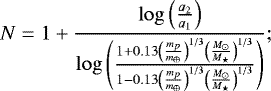
We refer to the work in Kervella et al. (2019) for a detailed derivation of the following relations. In summary, for a target with parallax ϖ and assuming m2 ≪ m1 the mass of the secondary can be expressed as
![Mathematical equation: \begin{equation*} m_{2}(r)=\frac{\sqrt{r}}{\gamma\,[P(r)/\delta t]}\, \sqrt{\frac{m_{1}}{G}}\, \frac{\Delta v_{\mathrm{T,G2}}}{\eta\,\zeta}, \end{equation*}](/articles/aa/full_html/2021/01/aa39541-20/aa39541-20-eq9.png) (7)
(7)
where r is the secondary’s orbital radius, G is the gravitational constant, and ΔvT,G2 is the norm of the linear tangential velocity of the PMa vector, expressed as
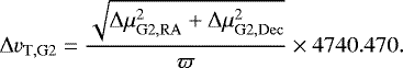 (8)
(8)
The proper motion measurement in the GDR2 catalogue is not an instantaneous measurement, but it is derived from a series of observations over a period of time δt of 668 days (Gaia Collaboration 2018). The measured PMa is then a time average over this time window, and the norm of the PMa is affected by observing window smearing depending on the ratio of the orbital period of the system P(r) to the observing time δt. This is accounted for using the γ factor, defined as
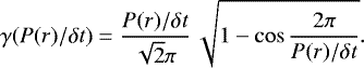 (9)
(9)
The possible inclination and position angle of the orbit can be approximated with the disc’s information (see Table 2) assuming a co-planar orbit. Thus, it is possible to deproject the PMa vector and evaluate the ratio η between the measured 2D PM vector projected onto the sky plane and the “real” 3D orbital PM vector. Normalising the observed PMa by η (which averages over orbital orientation and eccentricities) allows an estimation of the deprojected distribution of the companion mass.
If the orbital period of the system is longer than the baseline time δtHG used for the determination of the long-term PM vector μHG (i.e. the time difference between the hipparcos and Gaia DR2 epochs), then the PMa is biased. This bias is taken into account with the ζ function, defined as
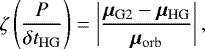 (10)
(10)
with P being the orbital period, and with δtHG ≃ 24.25 yr. Since no information on the orbital period is available, this is computed for every radial separation. Kervella et al. (2019) computed the proper motion anomaly for all the stars common to both the hipparcos and the Gaia DR2 catalogue, and suggested that a PMa S/N value >3 is an an indicator of the presence of a companion.
There are three targets in our survey that fit in this category: HD 161868, HD 8907, and HD 113337. Using the mass information from Table 1, the disc’s inclination and position angles from Table 2, and the parallaxes from Gaia DR2 and the PMa RA and Dec values from Kervella et al. (2019) (see Table 6), we computed the combinations of secondary mass and orbital radius that would explain the observed PMa.
In Figs. 7–9, we show these (m2,r) combinations (red line) with the respective 1, 2, and 3σ uncertainties (progressively lighter red shaded areas). We compared these possible companions with our achieved contrast curves, shown as a solid black line for the 5σ curve, together with the 3σ (dashed black line) and 1σ (dotted black line) curves. We also plot the position and extension of the resolved disc (blue dotted line and shaded area). The double-belt system HD 161868 is the only target for which only the inner belt is located in the field of view, and for this reason the dashed blue line in Fig. 7 represents the position of the inner belt, and not the resolved one, while the blue shaded area represents the uncertainties on the inner belt’s position and not its physical extent.
As visible in Fig. 7, the mass limits achieved for HD 161868 allow us to exclude the presence of planets more massive than a few tens of MJup beyond ~20 au, and to reasonably exclude objects more massive than 100 MJup between 10 and 20 au. Together with the presence of a disc at ~30 au, we can exclude the presence of planets massive enough to be responsible for the observed PMa at those radial separations. Moreover, there are no known massive companions further away that could explain the PMa; two candidate companions were detected at ~ 6′′.1 and ~ 7′′.2 by Janson et al. (2013), but they were ruled out as background stars. The minimal planetary system responsible for clearing the disc gap (see Sect. 5.2) would not be necessarily responsible for the PMa, unless one of them has a particularly high mass. We then suggest that the observed anomaly can be explained either by a very close-in (<2 au) unknown stellar companion or by an as-yet- undetected low-mass stellar companion with an orbital radius between 2 and 10 au and a mass of ≥100 MJup, just below our DI detection limits.
Regarding HD 8907 (Fig. 8), our imaging observations can reasonably exclude the presence of companions more massive than ~10 MJup beyond ~15 au, while the resolved disc’s information can exclude the presence of companions between ~ 30 and ~ 80 au. We did not find any known further away companion in the literature, and we therefore suggest that the observed anomaly could be caused by a currently undetected planetary companions with an orbital radius <15 au and a mass of ~ 10 MJup. The observed PMa could also be explained by a currently unknown stellar companion at periods that are, for example, near one-half, one-third, and one-fourth of the DR2 observing window, which correspond to a semi-major axis of ~ 0.8, ~ 1, and ~ 1.5 au (see Fig. 8).
Finally, we discuss the case of HD 113337, shown in Fig. 9. The presence of a resolved disc combined with our achieved mass detection limits allow us to exclude companions more massive than ~ 30 MJup beyond 20 au. HD 113337 has a known M3.5 dwarf companion, far away at ~ 200′′.0 (according to the Washington Double Star Catalog; see Mason et al. 2014), but neither this object nor the close-in companion at ~ 1 au is massive enough to explain the observed anomaly. The companion candidate at ~ 5 au (detected via RV; see Borgniet et al. 2019a) would have a mass compatible with the observed proper motion anomaly; we suggest that this finding points towards the confirmation of the RV signal and the presence of an additional planet in this system.
Additional RV observations for all of these three targets might help to shed light on these systems, particularly in the framework of excluding (or detecting) very close-in stellar mass companions, thus helping to shrink the parameter space.
Proper motion: anomalous values.
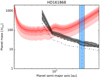 |
Fig. 7 Proper motion anomaly analysis from Kervella et al. (2019) for HD 161868. The red line is the relation between the companion’s mass (in Jupiter masses) and orbital radius (in au) that can explain the observed PMa, and the red shaded areas (progressively darker) are the 1, 2, and 3σ uncertainties. The black solid line and black shaded area denote the achieved 5σ mass detection limits from the LIStEN observations with its uncertainty, together with the 3σ (dashed line) and 1σ (dotted line). The blue dashed line and shaded area represents the position and uncertainty of the inner belt derived via SED fitting. The position of the resolved outer belt of HD 161868 is not visible in the field of view. |
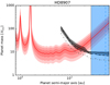 |
Fig. 8 As in Fig. 7. The blue dashed line and shaded area represents the resolved disc position and extent for HD 8907. |
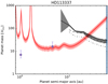 |
Fig. 9 As in Fig. 7. The blue dashed line and shaded area represents the resolved disc position and extent for HD 113337. The purple points and error bars indicate the position and mass of the two known RV planets orbiting the star (seeTable 2). |
6 Summary and conclusions
6.1 Summary
In this paper we have presented the LIStEN survey in terms of its scientific goals, target selection, observations, data reduction, and data analysis. The goal of the survey is to detect and characterise the population of giant planets around circumstellar disc hosting targets, with a focus on investigating companion-disc interactions. The survey is designed to be complementary to the ISPY survey in the northern hemisphere. To this end, we selected nearby stars with signs of a circumstellar disc (either inferred via SED fitting or with a resolved disc image), and we prioritised targets for which the disc has been imaged, and those with known planetary companions, either revealed by the RV technique or conventional imaging. We ended up with a flexible master list from which we drew our targets depending on the allocated observing nights.
We observed 28 targets between October 2017 and April 2019: 18 single-belt DD targets, 4 double-belt DD systems, 4 PPD stars, and 2 for which the IR excess turned out to be non-significant. In this paper we have presented the observations, data reduction, and image inspection for all of them, but have focused the image analysis only on the confirmed 22 DDs, and we refer to an upcoming ISPY paper for the analysis of the 4 PPD targets. Of these 22 DD targets, 14 have a resolved disc and 5 have known companions (4 targets have companions discovered via RV observations, and 1 target has a known imaged companion at a very large angular separation).
All the targets were observed in ADI dual mirror mode (whenever possible; see Table 3) with the LMIRCam instrument at LBT, observing each star through meridian passage with the goal of obtaining a minimum field rotation of 60°. During the data reduction and analysis we kept the data from the two mirrors separated, taking advantage of these semi-independent simultaneous observations to distinguish between speckles and physical candidates during the data inspection phase. All the data were reduced with our own semi-automated pipeline, and analysed with the PynPoint package. No new companion candidate was detected.
We produced 5σ contrast curves for all the DDs targets, reaching a median contrast of ~ 5 mag at 0′′. 2 and a background limit of ~ 10 mag at separations > 1′′.5. We evaluated the detection space for the survey converting the contrast curves into mass limits using known evolutionary models, and then we ran MC simulations of 107 planets per star, with randomised masses and orbital parameters, assessing which planet would have been discovered given the achieved mass limits. We achieve a detection probability greater than 50% for companions with masses ≥30 MJup between 30 and 100 au.
We used our achieved mass limits and the debris disc information to place constraints on the presence of undetected planets around eachtarget. Following the work from Krivov & Booth (2018), we tested the hypothesis that self-stirring alone can explain the size of the debris discs, and we found out that this is true for all the targets; for the four double-belt systems we tested this hypothesis on the outer belt. However, we note that self-stirring models are strongly dependent on the age of the system, which is often a non-straightforward parameter to derive and can have significant uncertainties. Moreover, for eight targets the only information on the disc comes from SED fitting, so the assumed radii may differ from the actual outer edge of the stirred disc. Obtaining resolved images of these discs, as well as better and more coherent constraints on the system’s age, will help to confirm (or reject) the self-stirring hypothesis.
We then focused on the four double-belt systems, and we used the work from Shannon et al. (2016) to derive the minimum mass planetary system needed to explain the position and radial extent of the gap between thetwo belts around each target. We find that the gap in these systems can be explained by the presence of multi-planetary systems (between four and six planets each) with masses ranging from ~ 25 to ~ 85 M⊕. These masses are several order of magnitudes lower than those achieved with our mass limits, and given the radial separations and planetary masses involved, current detection methods such as imaging and radial velocity cannot at the present time probe this parameter space.
Finally, three targets in our survey show an anomaly in the proper motion when comparing the Gaia DR2 data and the hipparcos data. Following the work in Kervella et al. (2019), we explored the parameter space of companion mass and semi-major axis that could explain the observed anomaly. Using disc information and our achieved mass limits we were able to constrain the mpl − apl parameter space, and we made predictions regarding the mass and semi-major axis of currently undetected companions around these systems, which can be used as a guide for future observations.
6.2 Conclusions
Future RV observations and direct imaging follow-ups will be able to test our predictions and shed more light on these interesting systems. At least three targets from the LIStEN survey would benefit from additional follow-up observations: HD 161868, HD 8907, and HD 113337. For HD 161868 and HD 8907, radial velocity observations would allow us to constrain the presence of an unseen massive companion within a few au, which could explain the observed proper motion anomaly; however, the early spectral type of HD 161868 might prove challenging for RV observations. For HD 113337 additional RV observations might confirm the second planetary candidate at ~ 5 au, and corroborate the hypothesis that the companion is real and responsible for the proper motion anomaly.
While the survey is considered completed and delivered interesting conclusions for single systems, the size of its target sample is too small to draw statistically meaningful conclusions on the matter of companion-disc interaction as a whole. Increasing this sample is therefore the primary goal, and efforts are needed to increase the number of resolved circumstellar discs (using such facilities as ALMA) and to obtain additional constraints on the presence of companions around stars with an already resolved disc, using both direct imaging and indirect detection techniques. At the moment of writing there are still a few tens of systems in the northern hemisphere for which the disc has been fully or partially resolved, but that still lack deep high-contrast imaging observations (and for which such observations would be feasible). Obtaining DI data for these objects should be a primary goal, and efforts to this end are currently ongoing. An example is the recently accepted proposal to use the LBT to obtain M-band ADI observations of four protoplanetary discs recently resolved by ALMA as part of the Disk Substructures at High Angular Resolution Project (DSHARP, Andrews et al. 2018). The proposal has the twofold goal of resolving these four discs in scattered light, and placing constraints on the presence of possible unseen companion candidates that might be responsible for the discs’ structure and morphology.
The NaCo-ISPY survey obtained deep DI data in the L′ band for more than 50 targets with a resolved debris disc. A companion-disc analysis for these targets, similar to that presented in Sect. 5, will be published in an upcoming NaCo-ISPY paper, as well as a joint analysis of the PPD targets from both surveys. In addition, occurrence rates for companions around disc-hosting stars (whether resolved or not) constitute another important piece of the puzzle, and to this end the LIStEN and NaCo-ISPY contrast curves and detection limits are planned to be combined for a joint statistical analysis of the occurrence rate of planetary and low-mass stellar companions around young nearby stars with debris discs.
Acknowledgements
We would like to thank the anonymous referee for the useful and constructive feedbacks. The LBT is an international collaboration among institutions in the United States, Italy and Germany. LBT Corporation partners are: The University of Arizona on behalf of the Arizona university system; Istituto Nazionale di Astrofisica, Italy; LBT Beteiligungsgesellschaft, Germany, representing the Max-Planck Society, the Astrophysical Institute Potsdam, and Heidelberg University; The Ohio State University, and The Research Corporation, on behalf of The University of Notre Dame, University of Minnesota and University of Virginia. We would like to thank Sascha Quanz for all the useful scientific discussions. We acknowledgethe use of the Large Binocular Telescope Interferometer (LBTI) and the support from the LBTI team, particularly Jordan Stone, Jennifer Power, Amali Vaz, Phil Hinz, Saavidra Perera, Kyle van Gorkum, Jennifer Lumbres and Ryan T. Webster. G.M.K. is supported by the Royal Society as a Royal Society University Research Fellow. T.H. acknowledges support from the European Research Council under the Horizon 2020 Framework Program via the ERC Advanced Grant Origins 83 24 28. T.D.P. is supported by DFG grants Kr 2164/14-2 and Kr 2164/15-2. This work has made use of data from the European Space Agency (ESA) mission Gaia (https://www.cosmos.esa.int/gaia), processed by the Gaia Data Processing and Analysis Consortium (DPAC, https://www.cosmos.esa.int/web/gaia/dpac/consortium). Funding for the DPAC has been provided by national institutions, in particular the institutions participating in the Gaia Multilateral Agreement. This research made use of Astropy (http://www.astropy.org), a community-developed core Python package for Astronomy (Astropy Collaboration 2013, 2018).
Appendix A Master flat and bad pixel mask creation
The LMIRCam is affected by vignetting, which can be seen as pixels around the border of the detector being substantially darker than the rest of the image. In addition to other possible bad pixels, there is also a known cluster of bad pixels roughly in the middle of the detector referred to as the “bullet hole”, which we carefully tried to avoid during observations and offsets. All of these issues make the creation of master flats and the handling of bad pixels a task that requires particular attention.
On October 8, 2017, we took a series of flat-field observations with DITs of 0.3, 0.7, 1., 1.4, 1.8, 2.1, 2.5, 2.9, and 3.2 s, taking 30 flats per DIT and then mean combining them, ending up with one flat per DIT. For each pixel we fit a linear relation as a function of DIT, saving all the resulting slopes. We then divided the highest DIT flat by the lowest DIT one, ending up with an array of ratios.
We flagged as “bad” all of those pixels that deviate more than a certain amount from the median of all ratios, thus creating a series of badpixel maps. We then inspected these maps by eye, to select the right trade-off between effectively masking the vignetting part and the bullet hole, and not labelling an overwhelming number of pixels as bad. We selected a deviation from the median-normalised ratios of 1.3 as our best trade-off. We used this mask while normalising the array of slopes, ending up with our master flat.
This procedure was applied to data taken in the 2017B run, with a detector window size of 2048 × 1280 pixels, and therefore the resulting master flat and bad pixel map can be used for every dataset taken with the same window size (i.e. for 2017B and 2018A run data). Due to work being done on the LMIRCam detector and the relative change in the vignetted area, we used a window size of 2048 × 1024 pixels for allthe data taken in the 2018B and 2019A run. Due to the different window size and to the possibly changed bad pixels, we created a new master flat and bad pixel mask for these data. The procedure is the same as explained for the 2017master flat creation, but we used a set of 80 frames with a DIT of 0.068 s, 80 frames with DIT of 0.109 s, and 40 frames with DIT of 0.302 s. The best trade-off for the bad pixel map was found with a deviation of 0.15.
We used a slightly less stringent bad pixel map during the bad pixel correction step in our data reduction: 1.5 deviation for the 2017B and 2018A data, and 0.25 deviation for the 2018B and 2019A data. During the star(s) location step, we sometimes used a very stringent bad pixel mask for some of our targets (usually the 0.15 or 0.10 deviation map) in order to completely avoid random hot pixels from being confused with the stellar peak(s).
5σ contrast curves for all the LIStEN targets.
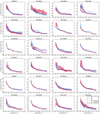 |
Fig. A.1 Comparison between the 5σ detection limits achieved using the unstacked and stacked frames for all the DD-hosting targets. Shown are the unstacked curves (in blue), together with their uncertainity (blue shaded area), and the limits and uncertainty achieved with the stacked frames (in red). The analysis is shown for both mirrors, left (SX; dashed line) and right (DX; solid line). |
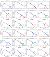 |
Fig. A.2 Flux density distribution of the DD-hosting targets for the LIStEN survey. The blue points are the photometric datapoints found in the literature, with blue triangles indicating upper limits. The black line is the IRS spectrum, while the green and red lines are the fitted stellar and disc fluxes, respectively. |
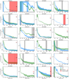 |
Fig. A.3 Achieved mass limits for all of the DD-hosting targets in the LIStEN survey. The blue line and blue shaded area represent the 5σ mass detection limit for the DX mirror with its lower and upper bound (estimated as the 25 and 75% quantiles). Similarly, the green line and green shaded area indicate the mass limit for the SX mirror. The red line and shaded area show the position (and uncertainty) for the resolved disc image (where applicable), while the black line and shaded area give the position of the SED-derived disc. If the system has two belts the inner one is shown as a dotted line and the outer one asa solid line. If the disc (either a single belt, one of two belts, or both belts) is not visible in the field of view, it is indicated with a red or black arrow (for the SED-inferred and resolved disc, respectively). |
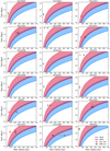 |
Fig. A.4 Self-stirring analysis for single-belt debris disc systems. The blue shaded area is the stirring timescale as a function of semi-major axis, according to Krivov & Booth (2018, KB18), while the red shaded area is that derived according to Kenyon & Bromley (2008, KB08). In both cases, the analysis encompasses two representative xm values of 1(dashed lines) and 10 (solid lines). The red and black points respectively represent the resolved and SED-inferred disc sizes at the estimated stellar age. |
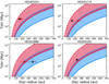 |
Fig. A.5 Self-stirring analysis for the double-belt debris disc systems. The analysis is done on the outer belt only, and the legend is the same as in Fig. A.4. |
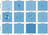 |
Fig. A.6 ADI reduced images of the targets observed in single-sided mode, for a representative PC number of 20. The images are oriented with north up, and the colour map was chosen to better visualise the data and bears no physical meaning. |
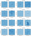 |
Fig. A.7 ADI reduced images of the targets observed in double-sided mode, for a representative PC number of 20. The images are oriented with north up, and the colour map was chosen to better visualise the data and bears no physical meaning. |
Appendix B Stacked versus unstacked frames
We evaluated 5σ detection limits for all of our DD targets using both unstacked and stacked frames (see Sect. 4). Given the computational time required to create contrast curves using the unstacked frames, we limited the analysis to a radial separation of 1′′. 4. We show the comparison between stacked and unstacked contrast curves (for both mirrors, when applicable) for a representative number of PC of 20 in Fig. A.1.
As can be seen in Fig. A.1, the detection limits are on average comparable between the stacked and unstacked frames, for both mirrors. For several targets, using stacked frames allows us to achieve a better detection limit at a given separation, with respect to the detection limit reached using the unstacked frames.
Given the results, we decided to use the stacked frames for the rest of the analysis since the achieved limits are comparable and the computational time is significantly reduced.
References
- Allard, F., Homeier, D., & Freytag, B. 2012, Phil. Trans. R. Soc. London Ser. A, 370, 2765 [Google Scholar]
- Amara, A., & Quanz, S. P. 2012, MNRAS, 427, 948 [NASA ADS] [CrossRef] [Google Scholar]
- Andrews, S. M., Huang, J., Pérez, L. M., et al. 2018, ApJ, 869, L41 [NASA ADS] [CrossRef] [Google Scholar]
- Astropy Collaboration (Robitaille, T. P., et al.) 2013, A&A, 558, A33 [NASA ADS] [CrossRef] [EDP Sciences] [Google Scholar]
- Astropy Collaboration (Price-Whelan, A. M., et al.) 2018, AJ, 156, 123 [Google Scholar]
- Bailer-Jones, C. A. L., Rybizki, J., Fouesneau, M., Mantelet, G., & Andrae, R. 2018, AJ, 156, 58 [NASA ADS] [CrossRef] [Google Scholar]
- Borgniet, S., Boisse, I., Lagrange, A. M., et al. 2014, A&A, 561, A65 [NASA ADS] [CrossRef] [EDP Sciences] [Google Scholar]
- Borgniet, S., Perraut, K., Su, K., et al. 2019a, A&A, 627, A44 [CrossRef] [EDP Sciences] [Google Scholar]
- Borgniet, S., Lagrange, A. M., Meunier, N., et al. 2019b, A&A, 621, A87 [NASA ADS] [CrossRef] [EDP Sciences] [Google Scholar]
- Bowler, B. P. 2016, PASP, 128, 102001 [NASA ADS] [CrossRef] [Google Scholar]
- Butler, R. P., Marcy, G. W., Vogt, S. S., et al. 2003, ApJ, 582, 455 [NASA ADS] [CrossRef] [Google Scholar]
- Chen, C. H., Mittal, T., Kuchner, M., et al. 2014, ApJS, 211, 25 [NASA ADS] [CrossRef] [Google Scholar]
- Cutri, R. M., Wright, E. L., Conrow, T., et al. 2013, Explanatory Supplement to the AllWISE Data Release Products [Google Scholar]
- David, T. J., & Hillenbrand, L. A. 2015, ApJ, 804, 146 [NASA ADS] [CrossRef] [Google Scholar]
- Dodson-Robinson, S. E., Su, K. Y. L., Bryden, G., Harvey, P., & Green, J. D. 2016, ApJ, 833, 183 [CrossRef] [Google Scholar]
- Ertel, S., Kennedy, G. M., Defrère, D., et al. 2018, SPIE Conf. Ser., 10698, 106981V [Google Scholar]
- Ertel, S., Defrère, D., Hinz, P., et al. 2020, AJ, 159, 177 [CrossRef] [Google Scholar]
- ESA 1997, VizieR Online Data Catalog: I/239 [Google Scholar]
- Fang, J., & Margot, J.-L. 2013, ApJ, 767, 115 [NASA ADS] [CrossRef] [Google Scholar]
- Feroz, F., Hobson, M. P., & Bridges, M. 2009, MNRAS, 398, 1601 [NASA ADS] [CrossRef] [Google Scholar]
- Gaia Collaboration (Brown, A. G. A., et al.) 2018, A&A, 616, A1 [NASA ADS] [CrossRef] [EDP Sciences] [Google Scholar]
- Grankin, K. N. 2016, Astron. Lett., 42, 314 [NASA ADS] [CrossRef] [Google Scholar]
- Hinz, P. M., Defrère, D., Skemer, A., et al. 2016, SPIE Conf. Ser., 9907, 990704 [Google Scholar]
- Holland, W. S., Matthews, B. C., Kennedy, G. M., et al. 2017, MNRAS, 470, 3606 [NASA ADS] [CrossRef] [Google Scholar]
- Husser, T., Wende-Von Berg, S., Dreizler, S., et al. 2013, A&A, 553, A6 [NASA ADS] [CrossRef] [EDP Sciences] [Google Scholar]
- Ishihara, D., Onaka, T., Kataza, H., et al. 2010, A&A, 514, A1 [NASA ADS] [CrossRef] [EDP Sciences] [Google Scholar]
- Janson, M., Brandt, T. D., Moro-Martín, A., et al. 2013, ApJ, 773, 73 [NASA ADS] [CrossRef] [Google Scholar]
- Jarrett, T. H., Cohen, M., Masci, F., et al. 2011, ApJ, 735, 112 [Google Scholar]
- Johnson, J. A., Howard, A. W., Marcy, G. W., et al. 2010, PASP, 122, 149 [NASA ADS] [Google Scholar]
- Kains, N., Wyatt, M. C., & Greaves, J. S. 2011, MNRAS, 414, 2486 [NASA ADS] [CrossRef] [Google Scholar]
- Kennedy, G. M., & Wyatt, M. C. 2014, MNRAS, 444, 3164 [NASA ADS] [CrossRef] [Google Scholar]
- Kennedy, G. M., Bryden, G., Ardila, D., et al. 2018, MNRAS, 476, 4584 [CrossRef] [Google Scholar]
- Kenyon, S. J.,& Bromley, B. C. 2008, ApJS, 179, 451 [NASA ADS] [CrossRef] [Google Scholar]
- Keppler, M., Benisty, M., Müller, A., et al. 2018, A&A, 617, A44 [NASA ADS] [CrossRef] [EDP Sciences] [Google Scholar]
- Kervella, P., Arenou, F., Mignard, F., & Thévenin, F. 2019, A&A, 623, A72 [NASA ADS] [CrossRef] [EDP Sciences] [Google Scholar]
- Krivov, A. V., & Booth, M. 2018, MNRAS, 479, 3300 [CrossRef] [Google Scholar]
- Lagrange, A.-M., Bonnefoy, M., Chauvin, G., et al. 2010, Science, 329, 57 [NASA ADS] [CrossRef] [PubMed] [Google Scholar]
- Launhardt, R., Henning, T., Quirrenbach, A., et al. 2020, A&A, 635, A162 [CrossRef] [EDP Sciences] [Google Scholar]
- Lebouteiller, V., Barry, D. J., Spoon, H. W. W., et al. 2011, ApJS, 196, 8 [NASA ADS] [CrossRef] [Google Scholar]
- Lehtinen, J., Jetsu, L., Hackman, T., Kajatkari, P., & Henry, G. W. 2016, A&A, 588, A38 [NASA ADS] [CrossRef] [EDP Sciences] [Google Scholar]
- Luhman, K. L., Patten, B. M., Marengo, M., et al. 2007, ApJ, 654, 570 [NASA ADS] [CrossRef] [Google Scholar]
- Lyubimkov, L. S., Rachkovskaya, T. M., Rostopchin, S. I., & Lambert, D. L. 2002, MNRAS, 333, 9 [NASA ADS] [CrossRef] [Google Scholar]
- Maire, A. L., Skemer, A. J., Hinz, P. M., et al. 2015, A&A, 579, C2 [CrossRef] [EDP Sciences] [Google Scholar]
- Marois, C., Lafreniere, D., Doyon, R., Macintosh, B., & Nadeau, D. 2006, ApJ, 641, 556 [Google Scholar]
- Marois, C., Macintosh, B., Barman, T., et al. 2008, Science, 322, 1348 [NASA ADS] [CrossRef] [PubMed] [Google Scholar]
- Marshall, J. P., Kirchschlager, F., Ertel, S., et al. 2014, A&A, 570, A114 [NASA ADS] [CrossRef] [EDP Sciences] [Google Scholar]
- Mason, B. D., Wycoff, G. L., Hartkopf, W. I., Douglass, G. G., & Worley, C. E. 2014, AJ, 122, 3466 [NASA ADS] [CrossRef] [Google Scholar]
- Mawet, D., Milli, J., Wahhaj, Z., et al. 2014, ApJ, 792, 97 [NASA ADS] [CrossRef] [Google Scholar]
- Meeus, G., Montesinos, B., Mendigutía, I., et al. 2012, A&A, 544, A78 [NASA ADS] [CrossRef] [EDP Sciences] [Google Scholar]
- Meshkat, T., Mawet, D., Bryan, M. L., et al. 2017, AJ, 154, 245 [NASA ADS] [CrossRef] [Google Scholar]
- Morales, F. Y., Rieke, G., Werner, M., et al. 2011, AAS Meeting Abstracts, 217, 339.08 [Google Scholar]
- Morales, F. Y., Bryden, G., Werner, M. W., & Stapelfeldt, K. R. 2016, ApJ, 831, 97 [NASA ADS] [CrossRef] [Google Scholar]
- Musso Barcucci, A., Launhardt, R., Kennedy, G. M., et al. 2019, A&A, 627, A77 [NASA ADS] [CrossRef] [EDP Sciences] [Google Scholar]
- Mustill, A. J.,& Wyatt, M. C. 2009, MNRAS, 399, 1403 [NASA ADS] [CrossRef] [Google Scholar]
- Paunzen, E. 2015, A&A, 580, A23 [NASA ADS] [CrossRef] [EDP Sciences] [Google Scholar]
- Pawellek, N. 2016, PhD thesis, University of Jena, Germany [Google Scholar]
- Pawellek, N., & Krivov, A. V. 2015, MNRAS, 454, 3207 [NASA ADS] [CrossRef] [Google Scholar]
- Perrier, C., Sivan, J. P., Naef, D., et al. 2003, A&A, 410, 1039 [NASA ADS] [CrossRef] [EDP Sciences] [Google Scholar]
- Rameau, J., Chauvin, G., Lagrange, A.-M., et al. 2013, ApJ, 772, L15 [Google Scholar]
- Reggiani, M., Christiaens, V., Absil, O., et al. 2018, A&A, 611, A74 [NASA ADS] [CrossRef] [EDP Sciences] [Google Scholar]
- Shannon, A., Bonsor, A., Kral, Q., & Matthews, E. 2016, MNRAS, 462, L116 [NASA ADS] [CrossRef] [Google Scholar]
- Skrutskie, M. F., Cutri, R. M., Stiening, R., et al. 2006, AJ, 131, 1163 [NASA ADS] [CrossRef] [Google Scholar]
- Skrutskie, M. F., Jones, T., Hinz, P., et al. 2010, Proc. SPIE, 7735, 1378 [Google Scholar]
- Steele, A., Hughes, A. M., Carpenter, J., et al. 2016, ApJ, 816, 27 [NASA ADS] [CrossRef] [Google Scholar]
- Stolker, T., Bonse, M. J., Quanz, S. P., et al. 2019, A&A, 621, A59 [NASA ADS] [CrossRef] [EDP Sciences] [Google Scholar]
- Stone, J. M., Skemer, A. J., Hinz, P. M., et al. 2018, AJ, 156, 286 [Google Scholar]
- Tamura, M. 2009, AIP Conf. Ser., 1158, 11 [NASA ADS] [CrossRef] [Google Scholar]
- Tokunaga, A. T. 2000, Infrared Astronomy, ed. A. N. Cox (New York: Springer), 143 [Google Scholar]
- Uyama, T., Hashimoto, J., Muto, T., et al. 2018, AJ, 156, 63 [NASA ADS] [CrossRef] [Google Scholar]
- Veyette, M. J., & Muirhead, P. S. 2018, ApJ, 863, 166 [NASA ADS] [CrossRef] [Google Scholar]
- Vogt, S. S., Butler, R. P., Marcy, G. W., et al. 2005, ApJ, 632, 638 [NASA ADS] [CrossRef] [Google Scholar]
- Wenger, M., Ochsenbein, F., Egret, D., et al. 2000, A&AS, 143, 9 [NASA ADS] [CrossRef] [EDP Sciences] [Google Scholar]
- Wright, E. L., Eisenhardt, P. R. M., Mainzer, A. K., et al. 2010, AJ, 140, 1868 [Google Scholar]
- Yelverton, B., Kennedy, G. M., Su, K. Y. L., & Wyatt, M. C. 2019, MNRAS, 488, 3588 [CrossRef] [Google Scholar]
- Zhou, Y., Apai, D., Metchev, S., et al. 2018, AJ, 155, 132 [NASA ADS] [CrossRef] [Google Scholar]
Number of planets discovered via DI by September 2020, data from the Extrasolar Planets Encyclopaedia at http://exoplanet.eu
The largest L′ band imaging survey from the LBT is, at the moment of writing, the Large Binocular Telescope Interferometer Exozodi Exoplanet Common Hunt (LEECH, Stone et al. 2018), which observed 98 stars with no target overlap with the LIStEN survey.
Obtained via private communication with Steve Ertel.
The targets were selected and observed prior to the release of the Gaia DR2, after which their distances were updated.
From the catalog of resolved debris discs, compiled and maintained at https://www.astro.uni-jena.de/index.php/theory/catalog-of-resolved-debris-disks.html
All Tables
All Figures
|
Fig. 1 Age, distance, and spectral type distributions for all the LIStEN targets. Distance uncertainties are smaller than the symbol size. Age uncertainties are not shown because they are derived in a non-homogeneous way and are not available for all targets. The stars are colour-coded according to their spectral type. The empty circles are the PPD targets. |
| In the text | |
|
Fig. 2 ADI reduced images of HD 206860 for both mirrors, for a representative PC number of 20. The images are oriented with north up and east left, and the colour map has been chosen to better visualise the data. The black arrow gives the position of a suspicious feature in the DX image, ruled out as a speckle thanks to the comparison with the SX image. |
| In the text | |
|
Fig. 3 ADI reduced image of HD 36112 (DX mirror only). The disc spirals are clearly visible. |
| In the text | |
|
Fig. 4 Contrast curves (5 σ) for all targets, and both mirrors where applicable (grey lines). The grey shaded area around each curve represents the 1 σ uncertainty range. The thick red line shows the median of all contrast curves. |
| In the text | |
|
Fig. 5 Survey detection probability as a function of companion mass and true (not projected) semi-major axis. |
| In the text | |
|
Fig. 6 Flux density distribution of HD 50554. The blue points are the photometric datapoints found in the literature, the black line is the IRS spectrum, and the green and red lines are the fitted stellar and disc fluxes, respectively. |
| In the text | |
|
Fig. 7 Proper motion anomaly analysis from Kervella et al. (2019) for HD 161868. The red line is the relation between the companion’s mass (in Jupiter masses) and orbital radius (in au) that can explain the observed PMa, and the red shaded areas (progressively darker) are the 1, 2, and 3σ uncertainties. The black solid line and black shaded area denote the achieved 5σ mass detection limits from the LIStEN observations with its uncertainty, together with the 3σ (dashed line) and 1σ (dotted line). The blue dashed line and shaded area represents the position and uncertainty of the inner belt derived via SED fitting. The position of the resolved outer belt of HD 161868 is not visible in the field of view. |
| In the text | |
|
Fig. 8 As in Fig. 7. The blue dashed line and shaded area represents the resolved disc position and extent for HD 8907. |
| In the text | |
|
Fig. 9 As in Fig. 7. The blue dashed line and shaded area represents the resolved disc position and extent for HD 113337. The purple points and error bars indicate the position and mass of the two known RV planets orbiting the star (seeTable 2). |
| In the text | |
|
Fig. A.1 Comparison between the 5σ detection limits achieved using the unstacked and stacked frames for all the DD-hosting targets. Shown are the unstacked curves (in blue), together with their uncertainity (blue shaded area), and the limits and uncertainty achieved with the stacked frames (in red). The analysis is shown for both mirrors, left (SX; dashed line) and right (DX; solid line). |
| In the text | |
|
Fig. A.2 Flux density distribution of the DD-hosting targets for the LIStEN survey. The blue points are the photometric datapoints found in the literature, with blue triangles indicating upper limits. The black line is the IRS spectrum, while the green and red lines are the fitted stellar and disc fluxes, respectively. |
| In the text | |
|
Fig. A.3 Achieved mass limits for all of the DD-hosting targets in the LIStEN survey. The blue line and blue shaded area represent the 5σ mass detection limit for the DX mirror with its lower and upper bound (estimated as the 25 and 75% quantiles). Similarly, the green line and green shaded area indicate the mass limit for the SX mirror. The red line and shaded area show the position (and uncertainty) for the resolved disc image (where applicable), while the black line and shaded area give the position of the SED-derived disc. If the system has two belts the inner one is shown as a dotted line and the outer one asa solid line. If the disc (either a single belt, one of two belts, or both belts) is not visible in the field of view, it is indicated with a red or black arrow (for the SED-inferred and resolved disc, respectively). |
| In the text | |
|
Fig. A.4 Self-stirring analysis for single-belt debris disc systems. The blue shaded area is the stirring timescale as a function of semi-major axis, according to Krivov & Booth (2018, KB18), while the red shaded area is that derived according to Kenyon & Bromley (2008, KB08). In both cases, the analysis encompasses two representative xm values of 1(dashed lines) and 10 (solid lines). The red and black points respectively represent the resolved and SED-inferred disc sizes at the estimated stellar age. |
| In the text | |
|
Fig. A.5 Self-stirring analysis for the double-belt debris disc systems. The analysis is done on the outer belt only, and the legend is the same as in Fig. A.4. |
| In the text | |
|
Fig. A.6 ADI reduced images of the targets observed in single-sided mode, for a representative PC number of 20. The images are oriented with north up, and the colour map was chosen to better visualise the data and bears no physical meaning. |
| In the text | |
|
Fig. A.7 ADI reduced images of the targets observed in double-sided mode, for a representative PC number of 20. The images are oriented with north up, and the colour map was chosen to better visualise the data and bears no physical meaning. |
| In the text | |
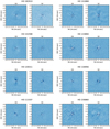 |
Fig. A.8 As in Fig. A.7 |
| In the text | |
Current usage metrics show cumulative count of Article Views (full-text article views including HTML views, PDF and ePub downloads, according to the available data) and Abstracts Views on Vision4Press platform.
Data correspond to usage on the plateform after 2015. The current usage metrics is available 48-96 hours after online publication and is updated daily on week days.
Initial download of the metrics may take a while.