| Issue |
A&A
Volume 667, November 2022
|
|
|---|---|---|
| Article Number | A63 | |
| Number of page(s) | 20 | |
| Section | Planets and planetary systems | |
| DOI | https://doi.org/10.1051/0004-6361/202244213 | |
| Published online | 08 November 2022 | |
Radial Velocity Survey for Planets around Young stars (RVSPY)
Target characterisation and high-cadence survey★
1
Max-Planck-Institut für Astronomie,
Königstuhl 17,
69117
Heidelberg, Germany
e-mail: This email address is being protected from spambots. You need JavaScript enabled to view it.
2
Main Astronomical Observatory, National Academy of Sciences of the Ukraine,
03143
Kyiv, Ukraine
3
Landessternwarte, Zentrum für Astronomie der Universität Heidelberg,
Königstuhl 12,
69117
Heidelberg, Germany
4
Instituto de Astrofísica, Pontifícia Universidad Católica de Chile,
Av. Vicuña Mackenna 4860,
7820436
Macul, Santiago, Chile
5
Astro-engineering center (AIUC), Instituto de Astrofísica, Pontifícia Universidad Católica de Chile,
Santiago, Chile
6
Space Telescope Science Institute,
3700 San Martin Drive,
Baltimore, MD
21218, USA
7
Universidad Andrés Bello, Departemento de Ciencias Fisicas, Facultad de Ciencias Exactas, Campus Casona de Las Condes, Astronomia,
Fernández Concha 700,
7591538
Santiago de Chile, Chile
8
Department of Physics, University of Warwick,
Coventry
CV4 7AL, UK
9
Centre for Exoplanets and Habitability, University of Warwick,
Gibbet Hill Road,
Coventry
CV4 7AL, UK
10
Indian Institute of Technology,
Madras, India
11
Department of Astronomy, Stockholm University, AlbaNova University Center,
SE-10691
Stockholm, Sweden
12
Department of Astronomy, Sofia University ’St Kliment Ohridski’,
5 James Bourchier Blvd,
1164
Sofia, Bulgaria
Received:
8
June
2022
Accepted:
5
August
2022
Abstract
Context. The occurrence rate and period distribution of (giant) planets around young stars is still not as well constrained as for older main-sequence stars. This is mostly due to the intrinsic activity-related complications and the avoidance of young stars in many large planet search programmes. Yet, dynamical restructuring processes in planetary systems may last significantly longer than the actual planet formation phase and may well extend long into the debris disc phase, such that the planet populations around young stars may differ from those observed around main-sequence stars.
Aims. We introduce our Radial Velocity Survey for Planets around Young stars (RVSPY), which is closely related to the NaCo-ISPY direct imaging survey, characterise our target stars, and search for substellar companions at orbital separations smaller than a few au from the host star.
Methods. We used the FEROS spectrograph, mounted to the MPG/ESO 2.2 m telescope in Chile, to obtain high signal-to-noise spectra and time series of precise radial velocities (RVs) of 111 stars, most of which are surrounded by debris discs. Our target stars have spectral types between early F and late K, a median age of 400 Myr, and a median distance of 45 pc. During the initial reconnaissance phase of our survey, we determined stellar parameters and used high-cadence observations to characterise the intrinsic stellar activity, searched for hot companions with orbital periods of up to 10 days, and derived the detection thresholds for longer-period companions. In our analysis we, have included archival spectroscopic data, spectral energy distribution, and data for photometric time series from the TESS mission.
Results. For all target stars we determined their basic stellar parameters and present the results of the high-cadence RV survey and activity characterisation. We have achieved a median single-measurement RV precision of 6 m s−1 and derived the short-term intrinsic RV scatter of our targets (median 23 m s−1), which is mostly caused by stellar activity and decays with an age from >100 m s−1 at <20 Myr to <20 m s−1 at >500 Myr. We analysed time series periodograms of the high-cadence RV data and the shape of the individual cross-correlation functions. We discovered six previously unknown close companions with orbital periods between 10 and 100 days, three of which are low-mass stars, and three are in the brown dwarf mass regime. We detected no hot companion with an orbital period <10 days down to a median mass limit of ~1 MJup for stars younger than 500 Myr, which is still compatible with the established occurrence rate of such companions around main-sequence stars. We found significant RV periodicities between 1.3 and 4.5 days for 14 stars, which are, however, all caused by rotational modulation due to starspots. We also analysed the data for TESS photometric time series and found significant periodicities for most of the stars. For 11 stars, the photometric periods are also clearly detected in the RV data. We also derived stellar rotation periods ranging from 1 to 10 days for 91 stars, mostly from the TESS data. From the intrinsic activity-related short-term RV jitter, we derived the expected mass-detection thresholds for longer-period companions, and selected 84 targets for the longer-term RV monitoring.
Key words: methods: observational / techniques: radial velocities / surveys / planets and satellites: detection / stars: activity / planetary systems
Tables A.1 and A.2 are only available at the CDS via anonymous ftp to cdsarc.cds.unistra.fr (130.79.128.5) or via https://cdsarc.cds.unistra.fr/viz-bin/cat/J/A+A/667/A63
© O. V. Zakhozhay et al. 2022
 Open Access article, published by EDP Sciences, under the terms of the Creative Commons Attribution License (https://creativecommons.org/licenses/by/4.0), which permits unrestricted use, distribution, and reproduction in any medium, provided the original work is properly cited.
This article is published in open access under the Subscribe-to-Open model.
This Open access funding provided by Max Planck Society.
1 Introduction
Within only a few million years, protoplanetary discs dissipate their gas due to accretion onto the star and newly formed planets, but also via disc winds and photoevaporation (e.g. Williams & Cieza 2011; Pascucci et al. 2022). By this time, most of the primordial dust has coagulated to pebbles and planetesimals or has been accreted onto forming planets. Collisional cascades within the disc then lead to the formation of debris dust. The size, mass, and brightness of the debris discs depend on the properties of the preceding protoplanetary discs (e.g. Najita et al. 2022). Relatively bright (Ld/L* ~ 10−4–10−2) and large debris discs with radii of up to a few 100au are observed around ~20–25% of low-mass (FGK) class III TTauri stars with ages between 5 and ~100 Myr (Hughes et al. 2018). During this time, that is to say after the initial planet formation, the planetary systems still evolve due to dynamical interactions and migration, but the central stars already experience much less chromospheric activity than at younger ages during the protoplanetary phase, such that planet searches become possible, albeit still challenging (e.g. Gregory 2017). However, many stars retain their debris discs much longer, albeit with slowly fading fractional luminosities reaching Ld/L* ~ 10−6–10−5 at few Gyr (Najita et al. 2022).
Several specific properties of debris discs such as the large inner gaps, the co-existence of cold outer and hot inner dust belts, or outer dust belts that are much larger than predicted by collisional cascade models, for example, may be explained by the action of newly formed planets (e.g. Moór et al. 2015). Thus, the observable properties of debris discs could be indicative of embedded and still evolving planetary systems. Yet, the relation between debris disc properties and the existence and properties of planets is still poorly understood. There are indications, albeit still debated, that the frequency of giant planets in young debris discs might be significantly higher than around main-sequence (MS) stars (e.g. Meshkat et al. 2017; Yelverton et al. 2020).
To systematically investigate the relation between debris disc properties and the occurrence of giant planets, the large direct Imaging (DI) Survey for Planets around Young stars (NaCo-ISPY) was initiated in 2015 (Launhardt et al. 2020). Since DI is only sensitive to companions at large separations (>5–10 au), we have launched a complementary systematic radial velocity (RV) survey for planets in closer orbits around these debris disc stars in 2017, using a Fibre-fed Extended Range Optical Spectrograph, mounted at the 2.2 m MPG/ESO telescope at ESO’s La Silla Observatory in Chile, Kaufer et al. 1999 (Sect. 4). Figure 1 illustrates the detection spaces of these two complementary surveys in terms of planet masses and semi-major axes.
This paper introduces our systematic RV Survey for Planets around Young stars (RVSPY) with debris discs, mainly targeting the giant planets and brown dwarfs in orbits shorter than seen by DI. The paper is organised as follows: In Sect. 2, we outline the motivation, goals, and general survey strategy. The targets and their properties are presented in Sect. 3. The observations and complementary data are described in Sect. 4 and the data reduction and analysis are described in Sect. 5. Results from the initial high-cadence observations are presented in Sect. 6 and discussed in Sect. 7. Section 8 summarises the paper.
2 Motivation, goals, and survey strategy
The main goal of the RVSPY survey is to help constraining the occurrence rate of Jovian-mass planets around low-mass stars with bright (detectable) debris discs. We aim to investigate the relation between the occurrence of such planets and the properties of the debris discs, which will provide important constraints for informing planet formation and evolution models that are used in planet population synthesis modelling. Since many main-sequence stars retain detectable debris discs for up to several Gyr, our survey is not restricted to young stars and thus contains age as an additional parameter to be tested.
Different planet detection methods have different detection biases and each method alone can explore only a certain part of the parameter space we are interested in. While DI is only sensitive to planets with large enough projected angular separations to be spatially resolved from the bright host star, RV has the opposite detection bias, that is, it is most sensitive to planets orbiting their host stars at small separations and with short orbital periods (Fig. 1). Thus, combining these two methods by designing this FEROS-RVSPY survey such that it has the largest possible target overlap with the NaCo-ISPY DI survey (Launhardt et al. 2020) will allow us to characterise the (giant) planet population around young debris disc stars over most orbital scales.
However, the two methods do not harmonise easily in all aspects. DI works best for young stars, when the planets are still hot from the formation process, and thus bright. Young stars in general rotate fast and the interplay between stellar rotation, convection, and magnetic fields, in particular in cool stars, leads to enhanced photospheric (e.g. star spots) and chromospheric (e.g. emission lines) activity. Both can alter the effective shape of spectral lines such that rotational modulation of line shapes due to activity features in the stellar atmosphere leads to an effective jitter (random or quasi-periodic) of the measured mean RV, which can mask or even mimic the RV modulation caused by an orbiting (planetary) companion (e.g. Hatzes 2002).
At very young ages, when a forming star efficiently accretes matter from the disc (i.e. for at most a few Myr), disc- and wind-locking mechanisms should keep its rotation speed low (e.g. Camenzind 1990; Matt & Pudritz 2005). When the accretion rate drops below some critical value, the star decouples from the disc and starts spinning up, owing to its ongoing contraction. However, stars less massive than approximately 1.3 M⊙ and cooler than Teff ≈ 6500 K (corresponding to a main-sequence spectral type later than F5) soon develop and maintain a convective envelope, in which dynamo processes generate a permanent magnetic field that causes the stars to spin down again via magnetic braking on a timescale of about 100 Myr (at 1 M⊙) to 1 Gyr (at <0.3 M⊙; Lamm et al. 2005; Irwin & Bouvier 2009; Weise et al. 2010; Bouvier et al. 2014). Consequently, such stars, when sufficiently slowed down, usually have many (because they are cool) and narrow (because they rotate slowly) absorption lines in their spectra and are thus well-suited for precision RV measurements. In stars more massive than about 1.3 M⊙, the dominating energy-efficient CNO cycle leads to the formation of a convective core and a radiation-dominated envelope in which no efficient dynamo can generate magnetic fields which could slow down the stellar rotation. These stars have not only fewer (because they are hotter), but also much broader spectral lines and are therefore less suited for precision RV measurements.
Hence, RV planet searches around young stars require one to carefully consider stellar ages, rotation velocity indicators (e.g. v sin(i)), and stellar spectral types (Teff) when defining the target sample and tailoring the observing strategy and cadence of the RV measurements. An efficient synergy between DI and RV planet searches is most promising for stars older than about 10 Myr, and for spectral types of F5 or later. Attention should be given to pre-main-sequence (PMS) stars younger than about 50 Myr, which are still contracting and heating up and may still rotate relatively fast even if their mass is below 1.3 M⊙. With these considerations we define our target selection criteria (Sect. 3.1), draw a suitable sub-sample from the ISPY target list, and extend it with more debris disc targets that were not observed within ISPY.
As outlined above, the target stars in question still exhibit stronger stellar activity than their more evolved MS counterparts. Rotational modulation of spectral line strengths and shapes due to activity-related stellar surface features causes signals that interfere with precise RV measurements. Therefore, it is mandatory to characterise the intrinsic stellar activity on the rotational time scales before attempting to search for RV variations that could be caused by orbiting companions. Rotational periods of young low- and intermediate-mass stars are well-explored and are typically constrained to periods between 1 and 10 days with a bimodal distribution peaking at ~8 days (slow rotators) and ~2 days (fast rotators; e.g. Herbst et al. 2002). The orbital period distribution of “hot Jupiters”, which are thought to have formed at larger separations in the discs and migrated inwards (e.g. Lin & Papaloizou 1986; Dawson & Johnson 2018), peaks in a similar range at 3–5 days.
Hence, with high-cadence RV measurement series covering about two weeks, with one to three spectra per night, we can both characterise the most significant activity-related variability of our targets as well as constrain the presence of hot companions (HC, which include hot Jupiters, with orbital periods ≤ 10 days). Although HC seem to be rare around ‘normal’ MS stars (0.4–1.2%; e.g. Santerne et al. 2016; Dawson & Johnson 2018; Zhou et al. 2019), it is not clear whether this also applies to young stars and to stars with massive debris discs. Since HCs induce much larger RV signals than longer-period planets, they are also easily detectable in Doppler data. Therefore, the initial phase of our FEROS-RVSPY survey is tailored to sample variability time scales of ~ 1–10 days to characterise stellar activity, while at the same time screening for the presence of HCs. The results and detection thresholds derived from this initial high-cadence survey are then used to identify those targets for which searching for longer-period companions (several months up to ~5 yr) seems feasible. In the second phase of the RV survey, which is not the subject of this paper, we continue to monitor the stars from this down-selected sample with an adapted lower cadence for up to a few years.
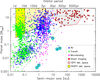 |
Fig. 1 Distribution of planet mass vs. orbital separation of confirmed exoplanets as listed on exopolanet.eu (January 2022, Schneider et al. 2011). Labelled on top are the corresponding orbital periods for M* = 1 M⊙ and Mp << M*. The main detection methods are marked by different colours. Solar System planets are represented by cyan circles and red letters. The horizontal dashed line marks the approximate deuterium burning mass limit. The solid yellow-shaded area marks the parameter space probed by our high-cadence RVSPY survey, assuming a conservative mean 3σ-sensitivity of 60 m s−1 (Sect. 6.2) and a mean stellar mass of 1 M0. The yellow-hatched area marks the extended detection space probed by our RVSPY survey assuming a long-term monitoring duration of 5 yr. The grey-shaded area marks the parameter space probed by the NACO-ISPY survey (10% detection probability, Launhardt et al. 2020). The light-grey dashed line marks the approximate detection threshold of current-day exoplanet searches. |
3 Targets
3.1 Target selection criteria
In accordance with our science goals and the specific complications outlined in Sect. 2, we restrict our target list to stars older than ~ 10 Myr, focus on young stars with ages of up to a few hundred million years, but do not apply a strict upper age limit, and restrict to stars that show a significant debris disc signature. This lower age limit is chosen to avoid the most active phase of young stars and the overlap with the preceding pro-toplanetary disc phase. Brems et al. (2019) show that the mean activity-induced RV jitter of young solar-type stars decreases from ≳500 m s−1 at 5 Myr to <200 m s−1 at 10 Myr, thus making age a crucial parameter for the target selection.
Spectral types are restricted to the range F6-M2, because earlier types have too broad and too few spectral lines (see Sect. 2), and later spectral types have too many spectral lines that blend. Furthermore, the latter are known to have less massive debris discs and fewer giant planets. We also set a brightness limit at V≤ 11 mag to limit individual exposure times. The declination range is naturally set to −75° ≤ Dec ≤ +25° by the location of the La Silla observatory. For some particularly interesting targets, the limits on declination and spectral type were not strictly obeyed. In particular we included a few stars with earlier spectral types (up to A7) to verify their v sin(i) and the achievable RV precision from test spectra before a decision was made to schedule them for high-cadence RV monitoring.
We also do not include in our target list stars for which a sufficiently large number of useable RV data was already available in archives. For this purpose, we have queried the ESO archive (FEROS, HARPS1) and the Keck archive (HIRES2). Stars with less than ten archival spectra are still kept in our survey list. Stars with ≥120 spectra are excluded, but we analyse their archival data in the same way as our own FEROS spectra and include the results in our final survey analysis. For stars with an intermediate number of archival spectra, we verify case by case whether sequences of spectra with sufficiently high cadence (see Sect. 4.1) are available and include or reject them from our survey list.
Also in accordance with our main science goals, we select our core target list for this RV survey from the target list of the NACO-ISPY survey (Launhardt et al. 2020), with the RV-specific selection criteria described above. This resulted in a list of 54 targets. However, for statistical reasons, in order to put robust constraints on the frequency of giant planets in debris discs and their relation to debris disc properties, one would ideally have a total sample size of ≥ 100 stars. We therefore enlarged our core target list by 57 additional targets selected from the Spitzer 1RS catalogue of Chen et al. (2014), and from Cotten & Song (2016) based on the criteria described above, although we verified the significance of the debris disc excess only later (see below, Sect. 3.2). Some of these stars were actually already included in the NACO-ISPY master target list, but could not be imaged in the end.
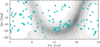 |
Fig. 2 Sky distribution of all 111 targets of this survey. The grey-shaded area and dotted contours outline the Milky Way disc and bulge as traced by the COBE-DIRBE band 2 (K) zodi-subtracted all-sky map (Hauser et al. 1989). |
3.2 Target properties
Our final target list for the survey observations consists of 111 stars, of which 54 stars were also imaged with NACO–ISPY (Launhardt et al. 2020). Figure 2 shows how the 111 targets are evenly distributed over the (southern) sky. Distances to all our stars are inferred from Gaia DR2 parallaxes (Gaia Collaboration 2016, 2018) with the method described by Bailer-Jones et al. (2018). Spectral types and V and K magnitudes are compiled from SIMBAD, the Hipparcos and Tycho Catalogues (van Leeuwen 2010; Høg et al. 2000), and from 2MASS (Cutri et al. 2003). For the 54 stars overlapping with ISPY (Launhardt et al. 2020), we adopt the stellar parameters from (Pearce et al. 2022). For the other 57 non-ISPY stars, we derive stellar parameters in the same way as described in this paper.
The stellar effective temperature Teff, bolometric luminosity L* of the stars, as well as the fractional luminosity and black-body temperature TBB of the associated debris discs3 are derived by fitting simultaneous stellar (PHOENIX; Husser et al. 2013) and blackbody models to the observed photometry and spectra as described in Launhardt et al. (2020) and Pearce et al. (2022). In this process, it turned out that 18 of the 57 non-ISPY stars selected from Chen et al. (2014) and Cotten & Song (2016) show only marginal or no significant debris disc emission4. The majority of these 18 stars are older than 1 Gyr, and nearly all are older than 500 Myr, as can be seen in Fig. 2. Since this was done only after the survey observations had started, these 18 stars are still included in our initial high-cadence survey, but they will neither be scheduled for longer-term monitoring (Sect. 4.1), nor will we use them for our anticipated statistical analysis of the occurrence of GPs around debris disc stars.
To derive stellar ages, we first checked each target for membership of known associations using the banyan Σ tool5 (Gagné et al. 2018). In addition, we checked if other youth indicators, such as vsin(i), are in agreement with the association age. If the membership probability was >80%6, and neither our isochronal age estimate, nor the measured vsin(i) contradict the association age, we assign the mean age of the association to the star. In total, we assigned association ages to 43 of our 111 stars. For the remaining 68 field stars, ages are assigned by compiling various literature estimates as described in Pearce et al. (2022). To validate our adopted ages, and to derive stellar masses, we also performed Hertzsprung–Russell diagram (HRD) isochrone fits as described in detail in Pearce et al. (2022). The resulting stellar masses were adopted for each star. The corresponding ages and uncertainties (which are naturally large for stars close to the main sequence) were not adopted. They were only used to verify the consistency of our adopted ages with the isochrone fits. Only for two stars, for which we could not find a valid literature age, we adopted the isochrone age directly. For most of the other stars, our adopted and isochronal ages agree to within 2σ. The uncertainties of our age estimates are discussed in Sect. 7.1.
Figure 3 shows the distribution of Teff, distances, stellar masses, luminosities, V magnitudes, and ages of all 111 survey targets. Effective temperatures range from 3800 to 7480 K (corresponding to spectral types A9 to MO, median 5840 K or Gl). Stellar masses range from 0.56 to 2.34 m⊙ (median 1.18 m⊙), v magnitudes from 3.7 to 10.6mag (median 7.8 mag), distances range from 6 to 160 pc (median 45 pc and one outlier with uncertain distance of 335 pc), ages range from 10 Myr to 7.6 Gyr (median 400 Myr), and bolometric luminosities range from 0.06 to 60 l⊙ (median 1.7 l⊙). The distance distribution is bimodal with a pronounced peak at 20–50 pc accounting for the most nearby stars within the local bubble, and a second peak 120–140 pc accounting for young stars associated to the nearest star-forming regions. Further target properties are derived in this paper from the FEROS spectra (Sect. 6.1). Target designations, coordinates, and most physical parameters mentioned above of all 111 survey stars are listed in Tables A.1 (debris disc stars) and A.2 (stars without a significant debris disc signal).
Figure 4 shows the HRD of our target stars with the stellar ages colour-coded. The main sequence is clearly visible. Also evident is a larger number of slightly overluminous pre-main sequence stars with ages below 25 Myr. Nearly all of these stars have significant infrared (IR) excess from debris discs. Furthermore, it can be seen that the very overluminous stars are actually old stars (giants) without significant IR debris disc excess.
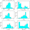 |
Fig. 3 Histograms showing the distributions of stellar effective temperatures (corresponding main-sequence spectral types marked on top), distances, masses, luminosities, V magnitudes, and ages of our survey targets. Dotted histograms show all 111 targets, while the blue filled histograms account only for targets with confirmed significant debris disc signal. |
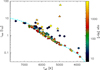 |
Fig. 4 HRD (L* vs. Teff) of single RVSPY target stars. Stellar ages are colour-coded. Stars marked as triangles do not have significant IR excess (see Sect. 3.1). To guide the eye, an updated version of the main sequence from Pecaut & Mamajek (2013) is marked by a dashed light-blue curve. |
4 Observations
4.1 Observing strategy
As outlined in Sect. 2, the first phase of our survey is designed to characterise the stellar activity jitter of all targets on the timescales of their rotational periods and to search for HCs. For this purpose, we scheduled every target star for one period of high-cadence observations consisting of 14–15 consecutive nights in which we obtained one spectrum per night during at least 13, ideally consecutive nights, plus 2–3 spectra per night during one to two nights. The order in which the stars during one such block were observed was changed from night to night and within their visibility time to avoid exact 24 h window function peaks in the periodograms, thereby probing the frequencies (or periodicities) relevant for both activity-related rotational modulation and hot companions.
Many of the more quiet stars in our sample exhibit an intrinsic RV scatter of <10 m s−1 (see Fig. 5), which is close to the instrumental limit of FEROS for stars with small v sin(i) and a sufficient number of narrow spectral lines, that is, cool stars. Such a precision can typically be achieved with an signal-to-noise ratio (S/N) ≳ 100. In practice however, the achievable RV precision also depends on the stellar spectral type, v sin(i), and the atmospheric conditions. Since the RV amplitude induced by a 1 MJup-mass planet in a 3-day orbit around a solar-mass star is about 50 m s−1, we aimed to identify and monitor only stars for which an intrinsic RV precision of σRV ≤ 50 m s−1 can be reached. In addition to the high-cadence observations, we took individual “test” spectra for stars that did not have any archival spectra available to assess their basic stellar parameters and the achievable RV precision (Sect. 3.2) and to decide whether or not they will be scheduled for high-cadence observations. The results and detection thresholds derived from this initial high-cadence survey were then used to identify those targets for which searching for longer-period companions (months up to 2–3 yr) seems feasible. In the second phase of the survey, we will continue to monitor the stars from this down-selected sample with an individually adapted lower cadence for up to a few years (see Sect. 7).
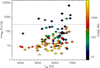 |
Fig. 5 Intrinsic rms scatter of the RVs in the 2-week high-cadence data vs. (spectroscopic) effective stellar temperature, Teff, with age encoded in colour. Stars marked as triangles do not have significant IR excess (see Sect. 3.1). The horizontal dashed-dotted line marks the approximate boundary above which we consider RV exoplanet searches not feasible (although we use a mass detection threshold in the end; see Sect. 7.5 and Fig. 11). |
4.2 High-cadence observations
During the first 3.5 observing years, between April 2018 and March 2022 (see Table 1), we obtained high-cadence time series of spectra for all our 111 survey targets. The observing campaigns typically consisted of about 14–15 consecutive nights.
All observations were carried out with the FEROS instrument, which provides a spectral resolution of R = 48000, high efficiency (~ 20%), and covers the wavelength range 350–920 nm. All spectra were taken in the “object-calibration” mode of FEROS with one fibre on the star and the second fibre observing simultaneously the “ThAr + Ne” calibration lamp. Standard calibration files (BIAS, FLATS, and lamp spectra for wavelength calibration “WAVE”) were taken before each observing night during the afternoon and reduced with the CERES pipeline (see Sect. 5.1 and Brahm et al. 2017a for details). To monitor the long-term stability of the spectrograph, we also observed a few RV standard stars during each campaign.
The required S/N ≥ 100 (Sect. 4.1) was achieved with integration times between 5 min for stars with V ≤ 6 mag and 20 min for stars with V = 10–11 mag. When the seeing exceeded 1.8″, the exposure time was increased. To ensure that the required S/N was actually achieved, and to identify possible spectroscopic binaries early on, we verified the data quality during the observations and analyse the RV time series after the first few observing nights of each run. During April – September of 2020 (observing semester p105) and April–July 2021 (observing semester p107), no observations were carried out due to the pandemic lockdown. The weather was good during most of the observing nights, with clear to thin cloud conditions and seeing mostly in the range 0″.6–1″.77 (median 1″). No observations were taken when the seeing exceeded 2.5″. About 10% of time was lost due to bad weather conditions (thick clouds or strong wind). Table 1 summarises the observing semesters.
Observing campaigns.
4.3 Complementary data
To extend the temporal baseline of the RV data of our targets and check if other high-cadence time series already existed for our targets, we looked for available archival spectra or already processed RVs that qualify for our purpose and can be combined with our own FEROS data. Archival FEROS spectra, which were not taken during our program, were downloaded from the RAW ESO Science Archive8 and reduced and analysed with the same procedure as we use for our own observing data. For 21 targets, we found precise Keck/HIRES RV data in the HIRES archive published in Tal-Or et al. (2019)9. In addition, we found precise HARPS RV data and activity indicators for 38 targets in the HARPS-RVBANK10 (Trifonov et al. 2020). However, since we found no existing high-cadence time-series dataset that qualifies for our purpose for any of our targets in the archives, we do not use these data here, but keep them for the longer-term follow-up survey, which is subject to a subsequent paper.
Furthermore, we used photometric time series data to derive additional constraints on stellar rotation periods and activity cycles. The majority of our targets are in the TESS11 observing list. For 91 of the 111 targets (82%), the TESS light curves are already publicly available and the data are retrieved, and included in our analysis.
To search for known indications of close companions to our targets, we evaluate the ninth catalogue of spectroscopic binary orbits (SB9; Pourbaix et al. 2004) and the Washington Visual Double Star Catalog (WDS; Mason et al. 2020). Close visual (i.e. not necessarily spectroscopically verifiable) companions are relevant for our study insofar as they can affect the photometry from which we derive certain stellar parameters (see Sect. 3.2). We also evaluated if our targets have significant (> 3σ) proper motion anomalies (PMa) between the long-term HIP–Gaia proper motion vector and the GDR2 measurements (PMaG2; Kervella et al. 2019), which could hint at the presence of (known and still unknown) close companions.
5 Data reduction and analysis
5.1 Tools
The basic reduction of the spectra and the extraction of RVs were done in a semi-automatic fashion with the CERES pipeline (Brahm et al. 2017a). CERES computes the RV of an observed spectrum by cross-correlating it with a binary mask for the stellar spectral lines. CERES provides three default masks for spectral types G2, K5, and M2. We used the mask that comes closest to the spectral type of a star (Tables A.1 and A.2).
The shape of the resulting cross-correlation function (CCF), which is also provided by CERES, is an important carrier of information about the origin of the measured RV variations (see below). For the computation of periodograms from time series data of RVs and various other quantities, we used the Generalised Lomb-Scargle (GLS) periodogram tool (Zechmeister & Kürster 2009), with the eccentricity fixed to zero and sine frequency (or period) output. For the extraction of stellar parameters, we used the ZASPE pipeline (Brahm et al. 2017b). To fit the RV data and derive the orbital parameters of the hypothetical companions we used The Exo-Striker fitting toolbox (Trifonov 2019).
5.2 Activity indicators
Stars generally exhibit higher levels of activity when they are young as compared to the rather quiet stage on the main sequence (e.g. Gregory 2017; Brems et al. 2019). Hence, possible planet signals in the RVs will always be accompanied by some degree of activity-related rotational modulation of the spectra, such that planet signals do not stand out as clearly. Their recovery requires, besides an adapted observing strategy (Sect. 4.1), both a special analysis strategy and a case-by-case treatment. These difficulties are also reflected in the unofficial nickname of our high-cadence survey, “Hot planets and rubble – let’s face the trouble”.
Rotational modulation of spectral line shapes due to activity features on the stellar surface can induce large RV scatter that can mask a planetary RV signal or even mimic it, when the spots are stable. To characterise the stellar activity and disentangle possible planetary signals from activity-induced RV variations, we derive activity-related parameters for all our observed spectra. In particular, Hα line indices (Kürster et al. 2003; Boisse et al. 2009), Ca II H&K Sindex (Duncan et al. 1991), line profile variations of Ca II H&K, Hα, Hβ, and Hγ (Johns & Basri 1995), line depth ratios of temperature-sensitive lines using line pairs (Biazzo et al. 2007), bisector shape, span (BS), displacement, and curvature (Povich et al. 2001) and full width at half maximum (FWHM) of the cross-correlation function derived by CERES. We determine stellar rotation periods (Prot) from time series of photometric data from TESS (Ricker et al. 2015).
To distinguish periodic RV variations caused by a physical companion from those that are related to rotational modulation of line shapes, we calculated both GLS periodgrams and linear correlations of all activity indicators with the RVs. In addition, to detect periodic variations of the line profiles or small parts of the lines, we calculated two-dimensional GLS periodograms for the Ca II H&K, Hα, Hβ, and Hγ lines (see Fig. B.2).
Depending on spectral type and age of the star, as well as geometrical aspects, chromospheric and photospheric activity can occur at different levels and might not be detectable equally in all indicators. For example, a well-established indicator to identify periodic rotational modulations of line shapes by dark spots on the stellar surface is the correlation between bisector span (BS) and RV. A strong anti-correlation between BS and RV is a clear indication of a dark spot (e.g. Queloz et al. 2001). However, depending on the inclination of the star, the spot latitude, and v sin(i), the strength of the correlation and the amplitude of the BS can vary significantly (e.g. Desort et al. 2007). It is therefore necessary to rely not only on one indicator, but to measure a variety of indicators of different origin and different sensitivities, especially in the case of a large RV survey.
We did not undertake this full activity analysis routinely for all targets, but only when we found a periodicity in the RV data that cannot be easily explained with fewer analyses. In Appendices B and C, we demonstrate as two examples our described activity analysis for targets HD 38949 and CPD-72 2713, for which most activity indicators show clear and unambiguous signals.
In addition, we used GLS periodograms of the photometric time series data from TESS (Sect. 4.3), where available, to independently derive photometric variability periods and draw conclusions on the most likely stellar rotational periods (Sect. 6.3). Knowing the stellar rotation periods helps us to interpret RV periodograms and to distinguish rotational modulation from companion-related RV variability (Sect. 6.2).
6 Results
We have obtained high-cadence time series of 19 spectra (median) over 12-20 days for all 111 stars of our survey. From the spectra, we determined the basic stellar physical parameters Teff, [Fe/H], and log(g)), and measured the rotation-dominated line broadening, v sin(i), and the activity-dominated short-term RV jitter, rmsRV(τ 14 d). We searched for RV periodicities on the 14-day timescale, and, where we found periodicities, analysed the correlation between RV and BS and compared the RV variability with the photometric variability in the TESS data where available. In addition, we used archival spectra where available to verify the longer-term RV variability.
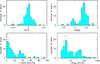 |
Fig. 6 Histograms showing the distributions of stellar metallicities [Fe/H], surface gravity log(g), v sin(i), and intrinsic rms scatter of the RVs in the 2-week high-cadence data (see Sect. 6.2). Dotted histograms show all 111 targets, while the blue filled histograms account only for targets with confirmed significant debris disc signal. |
6.1 Spectroscopic stellar parameters
In addition to the target properties presented in Sect. 3.2, we derived in this paper from our FEROS data spectroscopic Teff, metallicity [Fe/H] ≡ log10[(Fe/H)]/(Fe/H)⊙, surface gravity log10(g), and projected rotational line broadening v sin(i), using the open source ZASPE pipeline (Brahm et al. 2017b). Since the derivation of uncertainties for individual stars within ZASPE is computationally very expensive, we computed them only for selected stars and extrapolate the uncertainties to the entire sample12. For Teff, we adopted a general 1 σ uncertainty of 124 K (see Sect. 7.1), with the exception of a few stars for which the rms scatter of the Teff derived from the individual spectra was larger. For v sin(i), we selected seven stars with v sin(i) coming closest to 3, 5, 10, 20, 30, 40, and 50 km s−1 to compute individual 1 σ uncertainties. Based on the computed uncertainties for these example cases, we derived an empirical fit of the form  , with a lower limit of 5% towards larger v sin(i), for all our targets, with the following exception. For values of v sin(i) < 3 km s−1, we can no longer distinguish between instrumental and rotational broadening of the spectral lines and adopted therefore a lower limit of 3 km s−1 (Reiners et al. 2012).
Figure 6 shows the distributions of stellar metallicities [Fe/H], surface gravity log(g), and v sin(i) as dervived from our FEROS spectra. The spectroscopically derived Teff mostly agree with the photometrically derived ones (Sect. 3.2) within 3σ, and the Teff distributions (Fig. 3) are indistinguishable. There are only four stars for which the relative difference is 3-5 σ, which are discussed in Sect. 7.1. Our FEROS/ZASPE-derived metallicities, [Fe/H], agree mostly within 3 σ with those derived by Gaspar et al. (2016) where those are available. There are only three stars for which the relative difference is larger (3.3–5 σ, see Sect. 7.1). We verified our results on ten or more different individual spectra for each of these stars, but obtained very consistent numbers. Our metallicities cluster around solar (zero, as expected) with only eight stars having |[Fe/H]| > 0.4. These “outliers” are discussed in Sect. 7.1. The distribution of surface gravities clearly shows the main-sequence peak around log(g) ~ 4.4 and a secondary peak around log(g) ~ 3.9, which encompasses both the youngest PMS stars with ages between 10 and 30 Myr as well as the few old (sub-)giant stars which mostly have no significant debris disc excess (see Sect. 3.2). The very few “outliers” are discussed in Sect. 7. The distribution of v sin(i) is also bimodal, with the first peak between v sin(i) ~ 0.5 and 20 km s−1 encompassing those stars for which magnetic braking is efficient, and the second peak between v sin(i) ~ 30 and 45 km s−1 encompassing stars for which magnetic braking does not act, that is, stars more massive than ~1.3 M⊙ (see Sect. 2 and discussion in Sect. 7.3). The five very fast rotating stars (v sin(i) > 50 km s−1) are all young with ages between 15 and 200 Myr. The distribution of rmsRV(τ 14 days) is discussed in Sect. 6.2. The individual values for Teff(sp), [Fe/H], log(g), v sin(i), and rmsRV(τ 14 d) are listed in Tables A.1 and A.2.
6.2 RV variability in the high-cadence data
To quantify the RV variability of our targets on a 2-week time scale, we first looked at the intrinsic rms scatter of the RVs, irrespective of whether there are periodicities in the RVs or not. We achieved a median single-measurement RV precision of 〈σRV〉 = 5.75 m s−1 (4.45 m s−1 for stars younger than 500 Myr and 13.1 m s−1 for older stars), and measured a median short-term intrinsic RV scatter,  of 23 m s−1 (44 m s−1 for stars younger than 500 Myr and 10 ms−1 for older stars). Figure5 shows rmsRV(τ14d) vs. the effective temperature, Teff, for all targets, except the SB’s (see Sect. 6.4). We observed three stars with rmsRV(τ 14 days) ≳ 1000 m s−1: HD 115820, HD 141011, and HD 145972. All three stars are very young (15–16Myr) and none of them shows any significant periodicity in the high-cadence RV data, although the dominant photometric TESS periods (see Sect. 6.3) in HD141011 (0.95 day) and HD 145972 (1.5 days) might be marginally seen in the RVs. However, both stars also show several smaller TESS periodgram peaks at periods between 0.2 and 0.7 day, which could be indicative of week pulsations that could explain the large RV jitter, since these periods are not temporarily resolved by the sampling of our RV data. This goes along with the notion by Grandjean et al. (2021) and the analysis of Lagrange et al. (2009) that the RV jitter in young A-F5 stars is dominated by pulsations.
For HD 115820 (A7V, 15 Myr), the star with the largest rmsRV(τ 14 d) of ~6.2 km s−1, the TESS data indicate several strong and sharp periods between 42 and 68 min, plus numerous fainter periodgram peaks at longer periods up to a few days. These can most likely be attributed to g-mode pulsations, which typically occur in δ Scuti stars (e.g. Breger 2000; Murphy 2015). These strong and very short-period pulsations appear as random ‘noise’ in our RV data and explain the large rmsRV(τ 14 days) of HD 115820.
Excluding these three young and very active stars with signs of pulsations, we observed intrinsic RV rms scatter values between 2.4 and ~800 m s−1, with a general trend of increasing scatter with increasing Teff and with youth. Using the stellar masses (Tables A.1 and A.2), we also derived the corresponding mass-detection limits for HC corresponding to 3 × rmsRV(τ 14 days) and list the respective values for P = 10 days in Table D.1. For P = 3 days, we achieved a median mass-detection limit for HC around stars younger than 500 yr of ~1.4 M⊙ (~0.3 M⊙ for older stars). RV searches for longer-period planets become unfeasible if the short-term RV scatter rms exceeds a value of ~300 m s−1 (conservative estimate), but we actually used these rmsRV(τ 14 days) values to calculate mass detection limits on longer-period companions and select the targets suitable for longer-term RV monitoring (Sect. 7.5).
To further evaluate the nature of the RV variability, we analysed the time series periodograms13, the correlation between BS and RV (Queloz et al. 2001), and the shape of the cross-correlation functions (CCF) for each star. We found a strong anti-correlation (rP ≤ −0.6)14 between BS and RV in the high-cadence data of 40 stars, all marked in TableD.1, indicating that stellar spots dominate the observed RV variability. We also found significant periods between 1.3 and 4.5 days in the RV data of 14 stars, which we list in Table D.1. Of these, the RV periods of 12 stars agree with photometric periods seen in the TESS data (Sect. 6.3). Nine of these show the aforementioned strong anti-correlation between BS and RV, suggesting that we have indeed detected the stellar rotation period and not an HC.
Two stars with significant RV periods of 3.6 days (HD107146) and 1.56days (HD219498) have no TESS data available (yet), but the corresponding BS/RV correlation factors of (rP ≤ −0.79) suggest that we also see spot-dominated RV variability and may have detected the stellar rotation period. Two more stars without TESS data show only marginally significant RV periods of 3.1 (HD 131156) and 6 days (HD 23340), respectively. Since they also show BS/RV correlation factors of (rP ≤ −0.7), we interpret their RV variability as tentative detection of the stellar rotation period. In 18 more stars, the main TESS period is also marginally detected in the RVs, indicating spot-dominated rotational modulation of the RVs. In none of the remaining 69 targets we detect a significant RV periodicity in the range 1–14 days, that is, we do not find an HC among our 111 target stars. The planet mass detection limits and search completeness for our high-cadence survey are shown in Fig. 7.
6.3 Photometric variability
TESS photometric time series data are available and retrieved for 91 of our 111 target stars. We employed GLS periodograms to search for significant photometric variability periods between 0.1 and 20 days. If more than one TESS observing sector was available (for 67 out of 91 stars), we analysed the individual sectors separately. If similar periodicities were detected in all sectors of a given star, we averaged the respective period values and GLS power and derived the uncertainty from the scatter between the individual sectors. In Table D.1, we list the up to three most significant periods together with their GLS periodogram power. All listed photometric periods are highly significant and have a false alarm probability (FAP) of << 10−4. We also list in Table D.1 our best estimate of the most likely stellar rotation period and assume a minimum uncertainty of 0.1 day. For stars that show large (>1 km s−1) unexplained rmsRV(τ 14 days), we also searched the TESS data for frequencies up to 300 day−1, corresponding to periods down about 5 min. These short periodicities are not related to the stellar rotation period, but to possible pulsations (see Sect. 6.2).
For 30 stars, we identified one single dominant photometric period of which we are confident that it is caused by a single dominant spot (group) and represents the stellar rotation period. For 29 stars, we identified two dominant periods with an approximate 2:1 period ratio, which we interpret as the result of two dominant spot groups, such that the longer of the two periods represents the most likely stellar rotation period. For many of these stars, a visual inspection of the light curves confirms that the shapes and strength of the clearly visible wiggles are indeed alternating. For seven stars, we identified two periods close together and adopt the mean as the most likely rotation period. For ten stars, we only found a range of significant periods, but cannot clearly identify a rotation period. For seven stars, we identified two dominant periods that are not in a 2:1 ratio and it is unclear which one represents the rotation period. Finally, five stars do not show any significant photometric periodicity.
As reported in Sect. 6.2, we further detected rotation periods for two more stars without TESS data based on their RV variability. In total, we thus derived confident estimates of stellar rotation periods for 59 stars, and uncertain guesses for 32 stars. Our derived rotation periods range from 0.9 to 11 days.
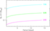 |
Fig. 7 Planet mass detection limits and search completeness for our high-cadence survey, corresponding to intrinsic rms scatter of the RVs in the 2-week high-cadence data. |
6.4 Spectroscopic companions
We identified nine spectroscopic binaries (SB) in our target list, of which only three were previously known. An orbit solution for HD 16673 (37-day nearly circular orbit with a m2 sin(i) ~ 0.2 m⊙ secondary) has been published only recently by Gorynya & Tokovinin (2018), after our survey had started. HD 27638 B has a relatively massive (mass ratio 0.85) seconday in a 17.6-d orbit (Tokovinin & Gorynya 2001), which we had obviously missed in our target selection. HD 141521 was previously identified as an SB2 by Weise et al. (2010), but no orbit solution has been published yet. We confirm the SB2 nature of this star, but cannot provide an orbit solution yet. None of these three stars shows a significant PMaG2.
In addition, we found six new SB, which were not reported previously. Since our high-cadence observations did not cover their full orbits, we can here only roughly estimate their orbital periods and secondary (minimum) masses and will publish the orbit solutions later. Three of these six stars have companions that are potentially in the brown dwarf mass regime with extrapolated orbital periods between 14 and 50 days (HD 102902, MML 43, and HD 129590). Of these, only HD 102902 shows a significant (4.8 σ) PMaG2 (Kervella et al. 2019) that would be consistent with a brown dwarf companion, albeit the orbital radius or period remain unconstrained. The orbital periods of the two other SB may be too short to detect such a PMa. HD 129590 has a bright nearly edge-on disc that was imaged in scattered light (Matthews et al. 2017; Olofsson et al. 2022).
Three other stars are found to have companions in the low-mass stellar regime with extrapolated orbital periods between 20 and 80 days (HD 20759, HD 108857, and HD 143811). Two of these also show a significant PMaG2 of 7.6 σ (HD 20759) and 3.5 σ (HD 108857), respectively, both consistent with low-mass stellar companions. Since these SB are not resolved spatially, their photometrically derived luminosities and Teff are also affected, which in turn affects the age and mass estimates derived from HRD isochrone fits (Sect. 3.2). We mark these stars in Tables A.1 and A.2 and discuss them in Sect. 7.1.
In addition to the nine targets with known or newly detected close (spectroscopic) companions mentioned above, we found eight more targets with significant (3.3–30 σ) PMaG2, but no other hints (yet) at the presence of a close companion. These stars are all marked in Tables A.1 and A.2. Since the PMaG2 has very little constraining power for orbital periods shorter than the Gαiα observing time window (668 d) due to observing window smearing (Kervella et al. 2019), and the longer-period RV variability and related PMa constraints are subject to a subsequent paper, we do not further discuss these sources with PMa here. We also do not consider the nine SB’s anymore in the following discussion since their photometric and spectroscpic properties are affected by the unresolved binarity.
7 Discussion
7.1 Uncertainties of stellar parameters
The median (1σ) uncertainty of the photometrically derived Teff is 70 K, that of the spectroscopically derived Teff is 110 K. Systematic uncertainties such as, for example, those caused by unresolved binarity, are not accounted for by these model uncertainties. The spectroscopically derived Teff are systematically higher by 124 K (median) than the photometrically derived ones, but they mostly agree with each other to within 3σ. This systematic difference is most likely related to the different synthetic model spectra used: while the spectral energy distribution (SED) fitting uses the PHOENIX models from Husser et al. (2013), ZASPE uses its own library of synthetic spectra (Brahm et al. 2017b). There are only three stars (not counting the SB) for which the relative difference is larger (3–5 σ), all very young (15 Myr) and with Teff > 6000 K. Of these, HD 114082 has a visual companion at 1″.5, which might have affected the photometry. HD 115820 shows a huge RV scatter rms of 6.3 km s−1, most likely owing to its δ Scuti-like pulsations (see Table D.1), which may also have affected derivation of Teff. HD 111520 (3.3 σ difference) also has a relatively large RV scatter rms of 220 m s−1, but has no known close companion and the spectra provide no hint at a SB. These slight Teff discrepancies might also be related to the limited applicability of the respective stellar atmosphere models used for such young stars.
Our literature-adopted and isochronal ages agree to within 2σ for all but four stars. For two supposedly young debris disc stars (HD 117524 and HD 141521, 15–16 Myr), our upper limit on the isochronal age is slightly more than 2σ below our adopted association age, but still within a factor of two only. These slight discrepancies can be easily explained by the large model uncertainties at these young ages, which are not accounted for by the formal fitting uncertainties. For two other stars (HD 5349, HD 102902, both without a significant debris disc signal), our isochronal fits suggest ages of below 5 Myr, while other studies classify them as Gyr old giant stars (Casagrande et al. 2011; Delgado Mena et al. 2019). Both stars have very small (unresolved) v sin(i), which suggests an old age. HD 102902 turns out to be a SB, that is, the blended photometry can explain the wrong isochronal age. For HD 5349, a closer look at the posterior distributions shows that both a 5 Myr old 1.75 M⊙ PMS star and an ~ 10 Gyr old 1.1 m⊙ K giant would be consistent with its location in the HRD. Based on the low v sin(i) and chemical (abundance rates) age derived by Delgado Mena et al. (2019), the Gyr age is however the more likely one.
Our stellar masses given in Tables A.1 and A.2 are derived from HRD isochrone fits to the MIST evolutionary models (Choi et al. 2016) and assuming a Chabrier (2003) single-star prior on mass (see Pearce et al. 2022). This, together with the fact that the photometry does not resolve SB, implies that the masses for SB and other close binaries (visual and those with a significant PMaG2) are not reliable. The respective stars are marked in Tables A.1 and A.2. Although we prefer our mass estimates over those of Kervella et al. (2019), because we use full SED evolutionary model fits and take metallicity into account, we compare our masses with those of Kervella et al. (2019), where available. We found on average good agreement with relative discrepancies rarely exceeding 20%, and only three stars exceeding the combined 3 σ significance level on the mass difference. These are HD 27638 B and HD 141521, which both are SB, and HD 117524, a very young (15 Myr) PMS star with a significant (20 σ) PMaG2, indicating the likely presence of a still unknown close companion.
Our FEROS/ZASPE-derived [Fe/H] are mostly consistent, within the error bars, with those derived by Gaspar et al. (2016). They differ by more than 3 σ (3.3–4.4σ, assuming a lower limit for the uncertainty of 0.1 dex) for only three stars. Two of these are actually SB, which means the quantities derived from the combined spectra might be wrong (HD 102902 and HD 141521). The third star is HD 191849, the lowest-mass M-dwarf in our sample. All three stars also belong to the group of eight stars with |[Fe/H]| > 0.4. The other five stars with |[Fe/H]| > 0.4 are HD 20759, which is also a SB, HD 5349, HD 101259, and HD 213941, which are all Gyr-old giants and for which our and the Gaspar metallicities are consistent with ours, and CPD-72 2713, a very young star (14Myr) which was not in the list of Gaspar et al. (2016).
Our FEROS/ZASPE-derived surface gravities indicate only six stars with log(g) < 3.7. Three of these are Gyr-old giants which we already excluded from further observations (HD 5349, HD 101259, and HD 138398). The three other stars log(g) < 3.7 are very young PMS stars (HD 115820, HD 117214, and CPD-722713), which explains their large radii and related low surface gravity.
7.2 RV precision as a function of Teff and vsin(i)
Here we investigate the relation between stellar effective temperature, Teff, projected rotational line broadening, v sin(i), and achievable RV precision, σRV. While v sin(i) directly affects the achievable RV precision, Teff is indirectly related to v sin(i) and σRV via the mechanisms discussed in Sect. 2. Figure 8 shows the relation between σRV and Teff, and v sin(i) for our target stars as derived from our FEROS spectra. There is a clear trend indicating that σRV increases with increasing Teff, although the scatter is large. All stars with Teff ≤ 6400 K have σRV ≤ 50 m s−1, which is the precision we aim for in our survey (Sect. 4.1). Many stars with higher Teff have significantly larger σRV, and not all of them are very young. This transition is actually close to the Teff limit above which magnetic braking is no longer efficient (Sect. 2). We used this coarse figure already to pre-select and prioritise those targets for which no values of v sin(i) (see below) were initially available from archival spectra or the literature, based on their Teff obtained from Gaia DR2 (Gaia Collaboration 2018) or from spectral energy distribution fits (Sect. 3.2). While stars with Teff ≤ 6000 K are in general safe targets, and stars with Teff ≥ 7500 K were not considered at all, selected stars with 6000 < Teff < 7500 K are scheduled for obtaining test spectra to characterise their v sin(i) and σRV before a decision is made about their inclusion in the survey.
The correlation between v sin(i) and σRV is significantly tighter and we derive a relation of log(σRV[m s−1]) = a (v sin(i)[km s−1]) + b with a = 0.071 and b = 1.35 for v sin(i) ≤ 40 km s−1, and a = 0.045 and b = 2.13 for v sin(i) ≥ 40 km s−1. The right panel of Fig. 8 shows that stars with v sin(i) ≤ 30 km s−1 all have σRV < 50 m s−1 and are thus safe survey targets, while stars with v sin(i) > 45 km s−1 all have σRV > 50 m s−1 are thus in general incompatible with our survey goals. Stars with intermediate values of v sin(i) require a case-by-case inspection of test spectra before a decision is made about their inclusion in the survey for longer-period companions.
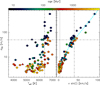 |
Fig. 8 Relation between single-measurement RV precision, σRV, and Teff (left) and v sin(i) (right). Stellar ages are colour-coded. Stars marked as triangles do not have significant IR excess (see Sect. 3.1). Horizontal dashed-dotted lines mark the anticipated threshold value for the RV precision of σRV = 50 m s−1 for our longer-term survey (Sect.4.1). Vertical dashed-dotted lines indicate the values of Teff = 6400 K (left panel) and v sin(i) = 40 km s−1 (right panel), above which many target are no longer compatible with our σRV ≤ 50ms−1 single-measurement RV-precision goal. The vertical dotted line on the right panel marks the lower sensitivity limit (3 km s−1) of our v sin(i) measurements (Sect. 6.1). The light-blue dashed lines in the right panel show the best linear fits to the correlation between v sin(i) and log(σRV) for v sin(i) ≤ 40 km s−1 and v sin(i) ≥ 40 km s−1. |
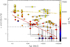 |
Fig. 9 Relation between v sin(i), age, and Teff for stars observed in the RVSPY high-cadence programme. Teff is coded in colour. Stars marked as triangles do not have a significant IR excess (see Sect. 3.1). Coloured dashed lines show separate linear fits to the relation between log(v sin(i)) and log(age) for stars with Teff < 6000 K (dark red) and stars with Teff > 6500 K (dark yellow). The horizontal dashed-dotted line marks the lower sensitivity limit of our v sin(i) measurements. |
7.3 Dependence of vsin(i) on age and Teff
We use the derived values of vsin(i) to analyse their mutual dependence on Teff and on the stellar age. Figure 9 shows the relation between v sin(i) and age for our targets, with Teff coded in colour. There is a clear correlation between Teff, v sin(i), and age. The hottest and youngest stars have the largest v sin(i), and the oldest and coolest stars have the smallest v sin(i). In addition, there seems to be a general v sin(i) offset between cool and hot stars. In accordance with the reasoning outlined in Sect. 2, we assume that this v sin(i) offset is related to the presence or absence of magnetic braking. We therefore perform separate fits to the relation log(v sin(i)[km s−1]) = a log(age[Myr]) + b. For the cooler stars with Teff < 6000 K, we derive a = −0.52 and b = 1.81, that is, they spin down with age much faster than stars with Teff > 6500 K, for which magnetic braking is inefficient and for which we derive a = −0.06 and b = 1.63. A comparison between Figs. 8 and 9 shows that all targets with Teff < 6000 K down to ages of 10 Myr are suited for RV measurements with the anticipated precision of 50 m s−1. Hotter stars with Teff > 6000 K may show too large v sin(i) for precise RV measurements when they are younger than 50–100 Myr, but each star must be checked individually since the scatter in the v sin(i) vs. age relation is large.
7.4 Dependence of short-term RV jitter on age
The median short-term intrinsic RV scatter, rmsRV(τ = 14 days), of our survey targets is 23 m s−1 (Sect. 6.2). Figure 10 shows the relation between rmsRV(τ = 14 days), derived in Sect. 6.2 (see also Fig. 5), and the stellar age. As expected for young stars with activity-related rotational modulation of line shapes and activity decaying with age, we find a relatively tight correlation, albeit with a number of outliers that show significantly larger RV jitter. These are mostly hot stars with Teff > 6000 K, which we have shown in Sect. 7.3 to not spin down but maintain a large v sin(i) even at older ages. These stars are not considered here.
For the remaining stars, our rmsRV–age relation agrees at large with the relation derived for a smaller sample by Brems et al. (2019).
However, our targets exhibit a slightly larger (factor ~2.6) rmsRV(τ = 14 days) than described by the relation of Brems et al. (2019), at least at ages > 50 Myr, where the scatter between individual targets is smaller than at younger ages. Adapting є in Eq. (5) of Brems et al. (2019) from 1.382 ± 0.041 to 0.93 would describe our sample better. This slightly larger mean RV jitter over 14 days in our data could be related to the larger size of our sample as compared to Brems et al. (2019, 111 vs. 27), to the ages they use (with only two stars in overlap, a direct comparison is not possible), or also to the fact that our rmsRV is in many cases derived from more than one high-cadence period, albeit after taking out the mean RV of the individual periods. Furthermore, since all timescales and stellar ages are fit with the same functional form, it is not surprising that discrepancies arise for larger parameter ranges than the ones used to derive this relation originally.
 |
Fig. 10 Relation between the intrinsic RV scatter, rmsRV(τ = 14days), age, and Teff for stars observed in the RVSPY high-cadence programme. Teff is coded in colour. Stars marked as triangles do not have significant IR excess (see Sect. 3.1). The black dashed line shows the relation derived by Brems et al. (2019, their Eq. (5) with parameters for model (a) from Table 3) for τ = 14 days. The thick orange dashed line shows the same relation with є modified from 1.382 to 0.93, adapted to our sample (see text). The horizontal dashed-dotted line marks the approximate boundary above which we consider RV exoplanet searches not feasible (although we use a mass detection threshold in the end; see Sect. 7.5 and Fig. 11). |
7.5 Identifying targets for longer-period planet search
The observations have already shown that, even with our careful target selection and the strategy for high-cadence observing campaigns, signatures of stellar activity and possible short-period companions are often not easy to disentangle and will require more data. Although we have not identified an HC in our sample from the high-cadence data, the data enable us to select those stars for dedicated follow-up observations that have a low-enough activity-related RV jitter to make searching for longer-period companions (P ≳30 days up to 5 yr) feasible.
Figure 11 illustrates the feasibility of target selection for such long-term follow-up observations with adapted cadence. We compute for all targets the minimum mass of a hypothetical companion that might still be detectable, assuming that the effective measurement precision is limited by the total RV scatter in the high-cadence data. These masses are computed assuming a 1-yr orbital period (as a proxy) and assuming that the required RV semi-amplitude is at least three times larger than the “activity noise” (rmsRV(τ = 14 days)). While we use this simplified assessment to select the targets for the longer-term RV-monitoring, we will try to reduce the observed short-term jitter for the longer-term data by fitting and subtracting the rotational RV modulation where the rotation period is known from TESS and evident in the RV data, as well as by fitting with a Gaussian process for correlated noise in the RVs.
Around eight stars, not counting the SB, we could only detect stellar-mass companions with periods of 1 yr. With the exception of HD 139664 (200 Myr), all these stars are younger than 20 Myr. These stars will not be followed up further for longer-period companions. We will also not follow up further the nine SB (Sect. 6.4), nor the 18 stars that turned out to show no or only marginal debris disc emission (Sect. 3.1). All these stars are marked in Table D.1. Around the remaining 84 stars, we could potentially detect longer-period brown dwarfs or even GPs (71 stars). While existing archival data allow us to derive constraints on longer-period companions for at least a subset of these 84 stars, the assessment of the longer-term RV variability, based both on archival and on our own FEROS data, will be subject of a subsequent paper.
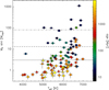 |
Fig. 11 Mass detection limits for hypothetical companions with P = 1 yr that induce an RV amplitude three times larger than the activity-jitter rms derived from the high-cadence observations, plotted vs. host star (spectroscopic) Teff. Ages are coded in colour. Stars marked as triangles do not have a significant IR excess (see Sect. 3.1). The horizontal dashed-dotted line marks the approximate boundary between the low-mass stellar and substellar regimes and the dashed line marks the approximate boundary between the planetary and brown-dwarf mass regimes. The dotted line marks 3 MJup. |
7.6 Comparison with other RV surveys
Dedicated RV surveys for planets around stars younger than a few hundred Myr are rare, although various larger surveys do not explicitly exclude young stars. Two of the most recently published relevant surveys by Grandjean et al. (2020, 2021) targeted 143 young (median age 150 Myr) nearby (median distance 28 pc) A0–M5 stars with the HARPS and SOPHIE15 instruments. Grandjean et al. (2021) also jointly analysed 120 of the stars in a statistical manner. Most of their targets are part of the SPHERE GTO programme “The SpHere INfrared survey for Exoplanets” (SHINE) survey sample (Chauvin et al. 2017). Grandjean did not explicitly target stars with debris discs and their sample extends to earlier spectral types (A stars) than our survey, although their median mass (1.0 M⊙) is the same as ours (Sect. 3.2). Correspondingly, 16 of their 120 targets are in common with our RVSPY target list. Their two surveys adopt slightly different observational strategies for late and early-type stars, but they also tried to sample both the short-term jitter as well as time baselines of several years. However, it is not well-described what the lengths and cadence of their high-cadence observing series is and how well stellar rotation periods and possible HCs are sampled.
Grandjean et al. (2021) measure a median short-term RV scatter of 50 m s−1 in their combined surveys, which compares well with the value of 44 m s−1 we measure for the younger half of our target list (Sect. 6.2, see also Sect. 7.4). No HC with P < 10 days was discovered in their surveys, but they discover one longer-period multi-GP system around HD 113337 (Borgniet et al. 2014, 2019b) and one additional long-period (P > 1000 days) sub-stellar companion candidate in the HD 206893 planetary system (Grandjean et al. 2019; Romero et al. 2021). In addition, they report three new spectroscopic binaries and confirm the binary nature of 13 stars. Except for HD 206893, none of their detections overlaps with our RVSPY target list. From the combined analysis of their two surveys, Grandjean et al. (2021) derive upper limits on the occurrence rates of GPs and BDs with periods between 1 and 1000 days around young A- to M-type stars of  and
and  , respectively. Also in accordance with their analysis is our finding that the RV jitter in several stars hotter than 6500 K and more massive than 1.3 M⊙ is dominated by pulsations, while the jitter in lower-mass stars is dominated by activity.
Grandjean et al. (2021) give a 90% completeness for HC in their survey down to 2–3 MJup and 50% completeness down to 0.2–0.4 MJup. Combining their results with our RVSPY high-cadence survey, we can conclude that in a sample of 135 stars with ages between 10 and 400 Myr, no HC was detected down a mean mass limit of ~0.5 MJup, which corresponds to a 68.3% confidence (1 − σ) upper limit on their occurrence rate of 0.9%. This is still consistent with the HC occurrence rate around older MS stars, which is in the range 0.4–1.2% (Sect. 2). Even the non-detection in all 210 targets of the combined surveys (without the SB), that is, ignoring age and assuming no evolution, would imply an upper limit occurrence rate of HC of 0.6%, which is still consistent with the HC occurrence rate around older MS stars reported by other studies.
Several large RV surveys for planets around MS stars were carried out and published during the past decade (e.g. Santerne et al. 2016; Borgniet et al. 2017, 2019a; Quirrenbach et al. 2020; Chontos et al. 2022). Not all of these were unbiased, but the most unbiased surveys report occurrence rates of HC in the range 0.4–1.2%, which if fully consistent with our finding of an 1 σ upper limit of 0.9%, that is, the same as for stars younger than 400 Myr (Sect. 6.2) since both age bins contain about half of our targets each.
8 Summary and conclusions
This paper presents the survey strategy, target list with stellar properties, and the results of the high-cadence reconnaissance observations of our RVSPY. Our survey list contains 111 stars of spectral types between early F and late K at distances between 6 and 160 pc (median 45 pc). About half of the targets are also part of the NACO DI survey for planets around young stars (NACO-ISPY; Launhardt et al. 2020).
Phase 1 of the RVSPY survey is dedicated to characterising the target stars and their activity, to search for HCs, and to select the targets for which searching for longer-period companions is feasible. During the high-cadence survey, all stars are observed in one or two two-week long observing campaigns with one or two spectra each night. All observations are carried out with the FEROS spectrograph (R = 48 000) at the La Silla observatory, in “object calibration” mode, and with integration times between 6 and 20 min. The main results for the stars observed during this first phase of our survey observations are summarised as follows:
We achieve S/Ns > 100 and a median single-measurement RV precision of 6 m s−1. The achievable RV precision strongly degrades with increasing Teff and v sin(i) and with decreasing age.
We derive the stellar parameters Teff, [Fe/H], log(g), and v sin(i) from the FEROS spectra. Values of Teff range from 3900 K to 7300 K with a median of 5900 K. Values of [Fe/H] cluster around solar (zero) with only eight stars having | [Fe/ H] | > 0. 4. The distribution of surface gravities shows the main-sequence peak around log(g) ~ 4.4 and a smaller secondary peak around log(g) ~ 3.9, which encompasses both the youngest PMS stars as well as a few old (sub-)giant stars. Values of v sin(i) range from <3 km s−1 to 90 km s−1 with a median of 7.7 km s−1. The distribution of v sin(i) is also bimodal, with the first peak between v sin(i) ~ 0.5 and 20 km s−1 encompassing those stars for which magnetic braking is efficient, and the second peak between v sin(i) ~ 30 and 45 km s−1 encompassing stars more massive than ~ 1.3 M⊙ for which magnetic braking does not act.
In addition, we derive stellar masses M* and luminosities L* from the SEDs. Stellar masses range from 0.56 to 2.34 M⊙ with a median 1.18 M⊙. Luminosities range from 0.06 to 60 L⊙ with a median 1.7 L⊙.
Stellar ages are derived via association with young moving groups (43 stars) and, for the remaining 68 field stars, from a combination of HRD isochronal fits and various literature ages derived with other methods. Our resulting ages range from 10 Myr to 7.6 Gyr with a median age of 400 Myr.
We find a clear trend with v sin(i) decreasing with increasing age, and a bifurcation between stars with Teff > 6000 K having significantly larger and slower decreasing v sin(i) than cooler stars, owing to their ability for magnetic breaking.
The median short-term intrinsic RV scatter, rmsRV(τ=14 d), of our survey targets is 23 m s−1 (44m s−1 for stars younger than 500 Myr and 10 m s−1 for older stars), with values ranging from about 2 m s−1 to 1.5 km s−1. The RV scatter for the majority of our targets is caused by stellar activity and/or pulsations (in stars more massive than 1.3 M⊙ or earlier than F5) and decays with age from >100 m s−1 at <20 Myr to <20 m s−1 at >500 Myr.
We analyse time series periodograms of the high-cadence RV data and find significant periods between 1.3 and 4.5 days for 14 stars. However, all these RV periodicities are clearly caused by rotational modulation due to starspots and we do not detect an HC with P < 10 days in our high-cadence RV data down to a median mass detection limit of ~1 MJup for stars younger than 500 Myr (0.3 MJup for older stars). Combining our result with the surveys analysed by Grandjean et al. (2021), we find an upper limit on the occurrence rate of HC around stars younger than 400 Myr of 0.9%, which is still consistent with the HC occurrence rate around older MS stars (0.4–1.2%).
We confirm three spectroscopic binary stars: HD 16673, HD 27638 B, HD 141521 (which were overlooked in the target selection), and report six previously unreported new spectroscopic binary stars with orbital periods between 10 and 100 days, but no orbit solutions yet. Three of these newly discovered companions have estimated minimum masses in the brown-dwarf regime (HD 102902, MML 43, and HD 129590), the other three in the low-mass-stellar regime (HD 20759, HD 108857, and HD 143811).
We also analyse the TESS photometric time series data for 91 of our target stars and find significant periodicities in nearly all of them. For 11 stars, the photometric periods are clearly detected also in the RV data. For 18 more stars, the photometric periods are marginally evident in the RV data.
For 91 stars, we derive stellar rotation periods (59 confident and 32 tentative), mostly from TESS data. The majority of our targets have rotation periods between 1 and 10 days (median 3.9 days).
From the intrinsic activity-related short-term RV jitter of our target stars, we derive the expected mass-detection thresholds for longer-period companions, and select 84 targets for the ongoing second phase of the survey.
The longer-term RV monitoring of our down-selected targets with individually adapted cadences, will go on for at least 2–3 more years.
Acknowledgements
The authors thank Didier Queloz, Andreas Quirrenbach, Nestor Espinoza, Raffael Brahm, Damien Ségransan, Carlos Eiroa, Amelia Bayo, Daniela Paz Iglesias Vallejo, Andres Jordan, and Jan Eberhardt for helpful discussions and feedback. O.Z. acknowledges support within the framework of the Ukraine aid package for individual grants of the Max-Planck Society 2022. A.M. acknowledges support of the DFG priority program SPP 1992 “Exploring the Diversity of Extrasolar Planets” (MU 4172/1-1)”. T.H. acknowledges support from the European Research Council under the Horizon 2020 Framework Program via the ERC Advanced Grant Origins 832428. G.M.K. is supported by the Royal Society as a Royal Society University Research Fellow. T.T. acknowledges support by the DFG Research Unit FOR 2544 ‘Blue Planets around Red Stars’ project no. KU 3625/2-1. T.T. further acknowledges support by the BNSF program “VIHREN-2021” project no. This work has made use of data from the European Space Agency (ESA) mission Gaia (https://www.cosmos.esa.int/gaia), processed by the Gaia Data Processing and Analysis Consortium (DPAC, https://www.cosmos.esa.int/web/gaia/dpac/consortium). Funding for the DPAC has been provided by national institutions, in particular the institutions participating in the Gaia Multilateral Agreement. This research has also made use of the SIMBAD database and the VizieR catalogue access tool, both operated at CDS, Strasbourg, France. The original description of the VizieR service was published in Ochsenbein et al. (2000). This paper includes data collected with the TESS mission, obtained from the MAST data archive at the Space Telescope Science Institute (STScI). Funding for the TESS mission is provided by the NASA Explorer Program. STScI is operated by the Association of Universities for Research in Astronomy, Inc., under NASA contract NAS 5–26555. We also wish to thank the anonymous referee for constructive criticism that helped to improve the clarity of the paper.
Appendix A Target list and basic stellar parameters
The Tables A.1 and A.2 are available at the CDS.
Appendix B Activity analysis of HD 38949
Here we demonstrate our stellar activity analysis and characterisation (as described in Sect. 5.2) which are exemplary for the star HD 38949. Figure B.1 shows (from top to bottom) the RV time series, the BS(RV) correlation, the GLS periodograms of the RVs and the photometric TESS16 data, as well as the photometric data time series. The two top panels show the two sets of available high-cadence FEROS data: blue - archival data, navy - RVSPY data. A significant linear correlation (rP = −0.92) between the BS and the RV indicates that the observed periodic RV variations are caused by surface features on the rotating star. The GLS periodogram of all available TESS photometric data shows two significant peaks at 3.8 d and 7.5 d, of which we assign the latter to the stellar rotation period, and the shorter one to a second dominant spot group on the opposite side of the stellar surface. The rotation period of HD 38949 was already estimated earlier from photometric measurements by Wright et al. (2011) to be ≈7.6 d, which agrees well with the longer period of the TESS photometry (see Table D.1). Two, albeit nonsignificant, periodogram peaks at similar periods are seen in the combined high-cadence RV data. The two additional and also non-significant peaks around 1 d are their daily aliases.
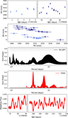 |
Fig. B.1 RVSPY and TESS data for HD 38949. The panels show (from top to bottom): the RV time series, the relation between RV and BS, the GLS periodograms of the RVs and of the photometric data (measured by TESS), and the TESS time series. All data products of the RVSPY programme are shown in black, all TESS data products are shown in red. Horizontal lines in the GLS periodogram of RVs reflect the 0.1%, 1% and 10% false alarm probabilities (from top to bottom). The corresponding false alarm probabilities of the TESS data GLS periodogram are all merged in the dashed line at the bottom of the periodogram, owing to the large number of the TESS data points. |
To further verify the hypothesis that we observe a RV variation which is caused by rotational modulation due to starspots, we compute two-dimensional versions of GLS periodograms for the spectral lines Ca II H&K and Hα by shifting all spectra to their rest wavelength and computing a periodogram for each velocity channel (Figs. B.2a though B.2c). These 2D periodograms show that all three line cores exhibit periodic variability on a time scale of about seven days. This subtle variability is not readily detected in the corresponding line EWs, which are integral quantities describing only the total intensity of the entire line. In addition, we also compute the S index and the Hα index (Sect. 5.2) and show the corresponding GLS periodograms in Figs. B.2d and B.2e. Similar to the line cores in the 2D periodograms, both quantities display significant variability on a time scale of 6–8 days, which agrees well with the longer of the two periods we find in both the TESS and the RV (albeit not significant) data. The additional 1 d period peaks in both GLS periodograms are the daily aliases of these signals. We therefore conclude for HD 38949 that the observed RV variations are dominated by rotational modulation due to starspots. This analysis also demonstrates the importance of using several indicators and methods simultaneously to identify and quantify processes related to stellar activity.
We perform a similar activity analysis for all stars in our sample in a semi-automatic fashion. Indeed, all 34 out of 40 stars with a clear anti-correlation between RV and BS (rP ≤ –0.6, Sect. 6.2) that have TESS data available show significant periodicities in the TESS photometric data (Sect. 6.3).
 |
Fig. B.2 (a-c) 2D GLS periodograms of Ca II K, H, and Hα. (d) GLS periodogram of the S -index based on flux measurements of Ca II H&K. (e) GLS periodogram of the Hα index. All three lines display a clear variability of HD 38949 on a time scale of 6–7 days. |
Appendix C Activity analysis of CPD–722713
A good example of a star with an interesting RV periodicity, that is not obviously doomed to be activity-related by a clear anti-correlation between RV and BS, is CPD–722713. This star was observed in high cadence in August 2018 and was initially classified as a ‘HC candidate’ because of a significant RV signal at PRV = 4.57 ± 0.10 d and the absence of a clear anti-correlation between RV and BS. However, a photometric study by Messina et al. (2017) reports a stellar rotational period of Prot = 4.46 d, which is very close to the RV period we find. The TESS data (released in December 2018) also confirm the presence of a significant signal at Pphot = 4.42 ± 0.002 d, which is clearly related to the rotational modulation caused by star spots. Hence, the periodic RV modulation is clearly related to the stellar rotation period and not to an orbiting companion.
Figure C.1 illustrates (from top to bottom) the RV time series, the BS(RV) (non-)correlation, the GLS periodograms of the RVs and the photometric TESS data, as well as the photometric data time series. The additional signal at a period of 1.3 d in the GLS periodogram of the RV data is an alias of the real signal at 4.57 d.
The absence of a clear BS/RV correlation in CPD–722713 is most likely related to the fact that the inclination of its rotation axis, derived from Prot, R*, and v sin(i), is ~78±4 deg, that is, the star is seen close to pole-on. At such high inclinations, the CCFs are just slightly shifted, but the CCF shape does not change with time, that is, the RVs are affected, but the bisectors are not (Desort et al. 2007), which explains the absence of a clear BS/RV correlation.
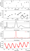 |
Fig. C.1 RVSPY and TESS data for CPD–722713. The panels show (from top to bottom): the RV time series, the relation between RV and BS, the GLS periodograms of the RVs and of the photometric data (measured by TESS), and the TESS time series. All data products of the RVSPY programme are shown in black, all TESS data products are shown in red. Horizontal lines in the GLS periodogram of RVs reflect the 0.1%, 1% and 10% false alarm probabilities (from top to bottom). The corresponding false alarm probabilities of the TESS data GLS periodogram are all merged in the dashed line at the bottom of the periodogram, owing to the large number of the TESS data points. |
Appendix D Additional Table
RV variability and periodicities in RV and TESS data
References
- Bailer-Jones, C. A. L., Rybizki, J., Fouesneau, M., Mantelet, G., & Andrae, R. 2018, AJ, 156, 58 [Google Scholar]
- Biazzo, K., Frasca, A., Catalano, S., & Marilli, E. 2007, Astron. Nachr., 328, 938 [NASA ADS] [CrossRef] [Google Scholar]
- Boisse, I., Moutou, C., Vidal-Madjar, A., et al. 2009, A&A, 495, 959 [NASA ADS] [CrossRef] [EDP Sciences] [Google Scholar]
- Borgniet, S., Boisse, I., Lagrange, A. M., et al. 2014, A&A, 561, A65 [NASA ADS] [CrossRef] [EDP Sciences] [Google Scholar]
- Borgniet, S., Lagrange, A. M., Meunier, N., & Galland, F. 2017, A&A, 599, A57 [NASA ADS] [CrossRef] [EDP Sciences] [Google Scholar]
- Borgniet, S., Lagrange, A. M., Meunier, N., et al. 2019a, A&A, 621, A87 [NASA ADS] [CrossRef] [EDP Sciences] [Google Scholar]
- Borgniet, S., Perraut, K., Su, K., et al. 2019b, A&A, 627, A44 [NASA ADS] [CrossRef] [EDP Sciences] [Google Scholar]
- Bouvier, J., Matt, S. P., Mohanty, S., et al. 2014, in Protostars and Planets VI, eds. H. Beuther, R. S. Klessen, C. P. Dullemond, & T. Henning, 433 [Google Scholar]
- Brahm, R., Jordán, A., & Espinoza, N. 2017a, PASP, 129, 034002 [Google Scholar]
- Brahm, R., Jordán, A., Hartman, J., & Bakos, G. 2017b, MNRAS, 467, 971 [NASA ADS] [Google Scholar]
- Breger, M. 2000, in Delta Scuti and Related Stars, eds. M. Breger & M. Montgomery, Astronomical Society of the Pacific Conference Series, 210, 3 [NASA ADS] [Google Scholar]
- Brems, S. S., Kürster, M., Trifonov, T., Reffert, S., & Quirrenbach, A. 2019, A&A, 632, A37 [EDP Sciences] [Google Scholar]
- Butler, R. P., Vogt, S. S., Laughlin, G., et al. 2017, AJ, 153, 208 [Google Scholar]
- Camenzind, M. 1990, Rev. Modern Astron., 3, 234 [NASA ADS] [CrossRef] [Google Scholar]
- Casagrande, L., Schönrich, R., Asplund, M., et al. 2011, A&A, 530, A138 [NASA ADS] [CrossRef] [EDP Sciences] [Google Scholar]
- Chabrier, G. 2003, PASP, 115, 763 [Google Scholar]
- Chauvin, G., Desidera, S., Lagrange, A. M., et al. 2017, in SF2A-2017: Proceedings of the Annual meeting of the French Society of Astronomy and Astrophysics, eds. C. Reylé, P. Di Matteo, F. Herpin, et al. [Google Scholar]
- Chen, C. H., Mittal, T., Kuchner, M., et al. 2014, ApJS, 211, 25 [Google Scholar]
- Choi, J., Dotter, A., Conroy, C., et al. 2016, ApJ, 823, 102 [Google Scholar]
- Chontos, A., Murphy, J. M. A., MacDougall, M. G., et al. 2022, AJ, 163, 297 [NASA ADS] [CrossRef] [Google Scholar]
- Cotten, T. H., & Song, I. 2016, ApJS, 225, 15 [Google Scholar]
- Cutri, R. M., Skrutskie, M. F., van Dyk, S., et al. 2003, VizieR Online Data Catalog: II/246 [Google Scholar]
- Dawson, R. I., & Johnson, J. A. 2018, ARA&A, 56, 175 [Google Scholar]
- Delgado Mena, E., Moya, A., Adibekyan, V., et al. 2019, A&A, 624, A78 [NASA ADS] [CrossRef] [EDP Sciences] [Google Scholar]
- Desort, M., Lagrange, A. M., Galland, F., Udry, S., & Mayor, M. 2007, A&A, 473, 983 [CrossRef] [EDP Sciences] [Google Scholar]
- Duncan, D. K., Vaughan, A. H., Wilson, O. C., et al. 1991, ApJS, 76, 383 [Google Scholar]
- Gagné, J., Mamajek, E. E., Malo, L., et al. 2018, ApJ, 856, 23 [Google Scholar]
- Gaia Collaboration (Prusti, T., et al.) 2016, A&A, 595, A1 [NASA ADS] [CrossRef] [EDP Sciences] [Google Scholar]
- Gaia Collaboration (Brown, A. G. A., et al.) 2018, A&A, 616, A1 [NASA ADS] [CrossRef] [EDP Sciences] [Google Scholar]
- Gaspar, A., Rieke, G. H., & Ballering, N. 2016, VizieR Online Data Catalog: J/ApJ/826/171 [Google Scholar]
- Gorynya, N. A., & Tokovinin, A. 2018, MNRAS, 475, 1375 [NASA ADS] [CrossRef] [Google Scholar]
- Grandjean, A., Lagrange, A. M., Beust, H., et al. 2019, A&A, 627, A9 [NASA ADS] [CrossRef] [EDP Sciences] [Google Scholar]
- Grandjean, A., Lagrange, A. M., Keppler, M., et al. 2020, A&A, 633, A44 [NASA ADS] [CrossRef] [EDP Sciences] [Google Scholar]
- Grandjean, A., Lagrange, A. M., Meunier, N., et al. 2021, A&A, 650, A39 [NASA ADS] [CrossRef] [EDP Sciences] [Google Scholar]
- Gregory, S. G. 2017, in Living Around Active Stars, eds. D. Nandy, A. Valio, & P. Petit, IAU Symposium, 328, 252 [NASA ADS] [Google Scholar]
- Hatzes, A. P. 2002, Astron. Nachr., 323, 392 [NASA ADS] [CrossRef] [Google Scholar]
- Hauser, M. G., Kelsall, T., Moseley, S. H., et al. 1989, BAAS, 21, 1219 [NASA ADS] [Google Scholar]
- Herbst, W., Bailer-Jones, C. A. L., Mundt, R., Meisenheimer, K., & Wackermann, R. 2002, A&A, 396, 513 [EDP Sciences] [Google Scholar]
- Høg, E., Fabricius, C., Makarov, V. V., et al. 2000, A&A, 355, L27 [Google Scholar]
- Hughes, A. M., Duchêne, G., & Matthews, B. C. 2018, ARA&A, 56, 541 [Google Scholar]
- Husser, T.-O., Wende-von Berg, S., Dreizler, S., et al. 2013, A&A, 553, A6 [NASA ADS] [CrossRef] [EDP Sciences] [Google Scholar]
- Irwin, J., & Bouvier, J. 2009, in The Ages of Stars, 258, eds. E. E. Mamajek, D. R. Soderblom, & R. F. G. Wyse, 363 [NASA ADS] [Google Scholar]
- Johns, C. M., & Basri, G. 1995, AJ, 109, 2800 [Google Scholar]
- Kaufer, A., Stahl, O., Tubbesing, S., et al. 1999, The Messenger, 95, 8 [Google Scholar]
- Kennedy, G. M., & Wyatt, M. C. 2014, MNRAS, 444, 3164 [NASA ADS] [CrossRef] [Google Scholar]
- Kervella, P., Arenou, F., Mignard, F., & Thévenin, F. 2019, A&A, 623, A72 [NASA ADS] [CrossRef] [EDP Sciences] [Google Scholar]
- Kürster, M., Endl, M., Rouesnel, F., et al. 2003, A&A, 403, 1077 [NASA ADS] [CrossRef] [EDP Sciences] [Google Scholar]
- Lagrange, A. M., Desort, M., Galland, F., Udry, S., & Mayor, M. 2009, A&A, 495, 335 [NASA ADS] [CrossRef] [EDP Sciences] [Google Scholar]
- Lamm, M. H., Mundt, R., Bailer-Jones, C. A. L., & Herbst, W. 2005, A&A, 430, 1005 [NASA ADS] [CrossRef] [EDP Sciences] [Google Scholar]
- Launhardt, R., Henning, T., Quirrenbach, A., et al. 2020, A&A, 635, A162 [NASA ADS] [CrossRef] [EDP Sciences] [Google Scholar]
- Lin, D. N. C., & Papaloizou, J. 1986, ApJ, 309, 846 [Google Scholar]
- Mason, B. D., Wycoff, G. L., Hartkopf, W. I., Douglass, G. G., & Worley, C. E. 2020, VizieR Online Data Catalog: B/wds [Google Scholar]
- Matt, S., & Pudritz, R. E. 2005, ApJ, 632, L135 [Google Scholar]
- Matthews, E., Hinkley, S., Vigan, A., et al. 2017, ApJ, 843, L12 [NASA ADS] [CrossRef] [Google Scholar]
- Mayor, M., Pepe, F., Queloz, D., et al. 2003, The Messenger, 114, 20 [NASA ADS] [Google Scholar]
- Meshkat, T., Mawet, D., Bryan, M. L., et al. 2017, AJ, 154, 245 [Google Scholar]
- Messina, S., Millward, M., Buccino, A., et al. 2017, A&A, 600, A83 [NASA ADS] [CrossRef] [EDP Sciences] [Google Scholar]
- Moór, A., Kóspál, Á., Ábrahám, P., et al. 2015, MNRAS, 447, 577 [Google Scholar]
- Murphy, S. J. 2015, A Pulsation Review of Delta Scuti and Related Stars (Cham: Springer International Publishing), 127 [Google Scholar]
- Najita, J. R., Kenyon, S. J., & Bromley, B. C. 2022, ApJ, 925, 45 [NASA ADS] [CrossRef] [Google Scholar]
- Ochsenbein, F., Bauer, P., & Marcout, J. 2000, A&AS, 143, 23 [NASA ADS] [CrossRef] [EDP Sciences] [Google Scholar]
- Olofsson, J., Thébault, P., Kral, Q., et al. 2022, MNRAS, 513, 713 [NASA ADS] [CrossRef] [Google Scholar]
- Pascucci, I., Cabrit, S., Edwards, S., et al. 2022, in Protostars and Planets VII, [arXiv:2203.10068] [Google Scholar]
- Pearce, T. D., Launhardt, R., Ostermann, R., et al. 2022, A&A, 659, A135 [NASA ADS] [CrossRef] [EDP Sciences] [Google Scholar]
- Pecaut, M. J., & Mamajek, E. E. 2013, ApJS, 208, 9 [Google Scholar]
- Pourbaix, D., Tokovinin, A. A., Batten, A. H., et al. 2004, A&A, 424, 727 [NASA ADS] [CrossRef] [EDP Sciences] [Google Scholar]
- Povich, M. S., Giampapa, M. S., Valenti, J. A., et al. 2001, AJ, 121, 1136 [NASA ADS] [CrossRef] [Google Scholar]
- Queloz, D., Henry, G. W., Sivan, J. P., et al. 2001, A&A, 379, 279 [NASA ADS] [CrossRef] [EDP Sciences] [Google Scholar]
- Quirrenbach, A., CARMENES Consortium, Amado, P. J., et al. 2020, SPIE Conf. Ser., 11447, 114473C [Google Scholar]
- Reiners, A., Joshi, N., & Goldman, B. 2012, AJ, 143, 93 [Google Scholar]
- Ricker, G. R., Winn, J. N., Vanderspek, R., et al. 2015, J. Astron. Telescopes Instrum. Syst., 1, 014003 [Google Scholar]
- Romero, C., Milli, J., Lagrange, A. M., et al. 2021, A&A, 651, A34 [NASA ADS] [CrossRef] [EDP Sciences] [Google Scholar]
- Santerne, A., Moutou, C., Tsantaki, M., et al. 2016, A&A, 587, A64 [NASA ADS] [CrossRef] [EDP Sciences] [Google Scholar]
- Schneider, J., Dedieu, C., Le Sidaner, P., Savalle, R., & Zolotukhin, I. 2011, A&A, 532, A79 [NASA ADS] [CrossRef] [EDP Sciences] [Google Scholar]
- Tal-Or, L., Trifonov, T., Zucker, S., Mazeh, T., & Zechmeister, M. 2019, MNRAS, 484, L8 [Google Scholar]
- Tokovinin, A. A., & Gorynya, N. A. 2001, A&A, 374, 227 [NASA ADS] [CrossRef] [EDP Sciences] [Google Scholar]
- Trifonov, T. 2019, Astrophysics Source Code Library [record ascl:1906.004] [Google Scholar]
- Trifonov, T., Tal-Or, L., Zechmeister, M., et al. 2020, A&A, 636, A74 [NASA ADS] [CrossRef] [EDP Sciences] [Google Scholar]
- van Leeuwen, F. 2010, Space Sci. Rev., 151, 209 [NASA ADS] [CrossRef] [Google Scholar]
- Vogt, S. S., Allen, S. L., Bigelow, B. C., et al. 1994, SPIE Conf. Ser., 2198, 362 [NASA ADS] [Google Scholar]
- Weise, P., Launhardt, R., Setiawan, J., & Henning, T. 2010, A&A, 517, A88 [NASA ADS] [CrossRef] [EDP Sciences] [Google Scholar]
- Williams, J. P., & Cieza, L. A. 2011, ARA&A, 49, 67 [Google Scholar]
- Wright, N. J., Drake, J. J., Mamajek, E. E., & Henry, G. W. 2011, ApJ, 743, 48 [Google Scholar]
- Yelverton, B., Kennedy, G. M., & Su, K. Y. L. 2020, MNRAS, 495, 1943 [Google Scholar]
- Zechmeister, M., & Kürster, M. 2009, A&A, 496, 577 [CrossRef] [EDP Sciences] [Google Scholar]
- Zhou, G., Huang, C. X., Bakos, G. Á., et al. 2019, AJ, 158, 141 [Google Scholar]
HARPS – High Accuracy Radial velocity Planet Searcher, mounted at 3.6 m telescope at La Silla observatory in Chile (Mayor et al. 2003).
HIRES – High Resolution Echelle Spectrometer, mounted on the 10 m Keck I telescope, USA, Hawaii (Vogt et al. 1994).
In this initial stage of our survey, we do not use the actual disc parameters yet, but only evaluate the significance of the disc excess to select the targets.
For most of these 18 stars, the issue appears to be related to the normalisation of the Spitzer 1RS spectra as discussed by Kennedy & Wyatt (2014, their Sect. 4.3)
For two stars with membership probabilities of 64 and 70%, we also assigned the mean age of the association because these ages are widely used in the literature and our isochronal ages did not contradict the association ages. These have corresponding notes in Table A.1.
Originally, this is the HIRES archive published by Butler et al. (2017), but corrected by Tal-Or et al. (2019) for small systematic errors in the RVs.
TESS – Transiting Exoplanet Survey Satellite (Ricker et al. 2015).
In the high-signal-to-noise regime, the uncertainty of the ZASPE-derived parameters is mainly determined by the mismatch between the observed and modelled spectra.
We use the Generalised Lomb–Scargle (GLS) periodogram tool by Zechmeister & Kürster (2009), with the eccentricity fixed to zero.
rP = Pearson correlation coefficient
Spectrographe pour l’Observation des Phénomènes des Intérieurs stellaires et des Exoplanètes.
Obtained from https://dx.doi.org/18.17989/t9-h5bx-p296.
All Tables
All Figures
|
Fig. 1 Distribution of planet mass vs. orbital separation of confirmed exoplanets as listed on exopolanet.eu (January 2022, Schneider et al. 2011). Labelled on top are the corresponding orbital periods for M* = 1 M⊙ and Mp << M*. The main detection methods are marked by different colours. Solar System planets are represented by cyan circles and red letters. The horizontal dashed line marks the approximate deuterium burning mass limit. The solid yellow-shaded area marks the parameter space probed by our high-cadence RVSPY survey, assuming a conservative mean 3σ-sensitivity of 60 m s−1 (Sect. 6.2) and a mean stellar mass of 1 M0. The yellow-hatched area marks the extended detection space probed by our RVSPY survey assuming a long-term monitoring duration of 5 yr. The grey-shaded area marks the parameter space probed by the NACO-ISPY survey (10% detection probability, Launhardt et al. 2020). The light-grey dashed line marks the approximate detection threshold of current-day exoplanet searches. |
| In the text | |
|
Fig. 2 Sky distribution of all 111 targets of this survey. The grey-shaded area and dotted contours outline the Milky Way disc and bulge as traced by the COBE-DIRBE band 2 (K) zodi-subtracted all-sky map (Hauser et al. 1989). |
| In the text | |
|
Fig. 3 Histograms showing the distributions of stellar effective temperatures (corresponding main-sequence spectral types marked on top), distances, masses, luminosities, V magnitudes, and ages of our survey targets. Dotted histograms show all 111 targets, while the blue filled histograms account only for targets with confirmed significant debris disc signal. |
| In the text | |
|
Fig. 4 HRD (L* vs. Teff) of single RVSPY target stars. Stellar ages are colour-coded. Stars marked as triangles do not have significant IR excess (see Sect. 3.1). To guide the eye, an updated version of the main sequence from Pecaut & Mamajek (2013) is marked by a dashed light-blue curve. |
| In the text | |
|
Fig. 5 Intrinsic rms scatter of the RVs in the 2-week high-cadence data vs. (spectroscopic) effective stellar temperature, Teff, with age encoded in colour. Stars marked as triangles do not have significant IR excess (see Sect. 3.1). The horizontal dashed-dotted line marks the approximate boundary above which we consider RV exoplanet searches not feasible (although we use a mass detection threshold in the end; see Sect. 7.5 and Fig. 11). |
| In the text | |
|
Fig. 6 Histograms showing the distributions of stellar metallicities [Fe/H], surface gravity log(g), v sin(i), and intrinsic rms scatter of the RVs in the 2-week high-cadence data (see Sect. 6.2). Dotted histograms show all 111 targets, while the blue filled histograms account only for targets with confirmed significant debris disc signal. |
| In the text | |
|
Fig. 7 Planet mass detection limits and search completeness for our high-cadence survey, corresponding to intrinsic rms scatter of the RVs in the 2-week high-cadence data. |
| In the text | |
|
Fig. 8 Relation between single-measurement RV precision, σRV, and Teff (left) and v sin(i) (right). Stellar ages are colour-coded. Stars marked as triangles do not have significant IR excess (see Sect. 3.1). Horizontal dashed-dotted lines mark the anticipated threshold value for the RV precision of σRV = 50 m s−1 for our longer-term survey (Sect.4.1). Vertical dashed-dotted lines indicate the values of Teff = 6400 K (left panel) and v sin(i) = 40 km s−1 (right panel), above which many target are no longer compatible with our σRV ≤ 50ms−1 single-measurement RV-precision goal. The vertical dotted line on the right panel marks the lower sensitivity limit (3 km s−1) of our v sin(i) measurements (Sect. 6.1). The light-blue dashed lines in the right panel show the best linear fits to the correlation between v sin(i) and log(σRV) for v sin(i) ≤ 40 km s−1 and v sin(i) ≥ 40 km s−1. |
| In the text | |
|
Fig. 9 Relation between v sin(i), age, and Teff for stars observed in the RVSPY high-cadence programme. Teff is coded in colour. Stars marked as triangles do not have a significant IR excess (see Sect. 3.1). Coloured dashed lines show separate linear fits to the relation between log(v sin(i)) and log(age) for stars with Teff < 6000 K (dark red) and stars with Teff > 6500 K (dark yellow). The horizontal dashed-dotted line marks the lower sensitivity limit of our v sin(i) measurements. |
| In the text | |
|
Fig. 10 Relation between the intrinsic RV scatter, rmsRV(τ = 14days), age, and Teff for stars observed in the RVSPY high-cadence programme. Teff is coded in colour. Stars marked as triangles do not have significant IR excess (see Sect. 3.1). The black dashed line shows the relation derived by Brems et al. (2019, their Eq. (5) with parameters for model (a) from Table 3) for τ = 14 days. The thick orange dashed line shows the same relation with є modified from 1.382 to 0.93, adapted to our sample (see text). The horizontal dashed-dotted line marks the approximate boundary above which we consider RV exoplanet searches not feasible (although we use a mass detection threshold in the end; see Sect. 7.5 and Fig. 11). |
| In the text | |
|
Fig. 11 Mass detection limits for hypothetical companions with P = 1 yr that induce an RV amplitude three times larger than the activity-jitter rms derived from the high-cadence observations, plotted vs. host star (spectroscopic) Teff. Ages are coded in colour. Stars marked as triangles do not have a significant IR excess (see Sect. 3.1). The horizontal dashed-dotted line marks the approximate boundary between the low-mass stellar and substellar regimes and the dashed line marks the approximate boundary between the planetary and brown-dwarf mass regimes. The dotted line marks 3 MJup. |
| In the text | |
|
Fig. B.1 RVSPY and TESS data for HD 38949. The panels show (from top to bottom): the RV time series, the relation between RV and BS, the GLS periodograms of the RVs and of the photometric data (measured by TESS), and the TESS time series. All data products of the RVSPY programme are shown in black, all TESS data products are shown in red. Horizontal lines in the GLS periodogram of RVs reflect the 0.1%, 1% and 10% false alarm probabilities (from top to bottom). The corresponding false alarm probabilities of the TESS data GLS periodogram are all merged in the dashed line at the bottom of the periodogram, owing to the large number of the TESS data points. |
| In the text | |
|
Fig. B.2 (a-c) 2D GLS periodograms of Ca II K, H, and Hα. (d) GLS periodogram of the S -index based on flux measurements of Ca II H&K. (e) GLS periodogram of the Hα index. All three lines display a clear variability of HD 38949 on a time scale of 6–7 days. |
| In the text | |
|
Fig. C.1 RVSPY and TESS data for CPD–722713. The panels show (from top to bottom): the RV time series, the relation between RV and BS, the GLS periodograms of the RVs and of the photometric data (measured by TESS), and the TESS time series. All data products of the RVSPY programme are shown in black, all TESS data products are shown in red. Horizontal lines in the GLS periodogram of RVs reflect the 0.1%, 1% and 10% false alarm probabilities (from top to bottom). The corresponding false alarm probabilities of the TESS data GLS periodogram are all merged in the dashed line at the bottom of the periodogram, owing to the large number of the TESS data points. |
| In the text | |
Current usage metrics show cumulative count of Article Views (full-text article views including HTML views, PDF and ePub downloads, according to the available data) and Abstracts Views on Vision4Press platform.
Data correspond to usage on the plateform after 2015. The current usage metrics is available 48-96 hours after online publication and is updated daily on week days.
Initial download of the metrics may take a while.