| Issue |
A&A
Volume 674, June 2023
|
|
|---|---|---|
| Article Number | A60 | |
| Number of page(s) | 19 | |
| Section | Stellar structure and evolution | |
| DOI | https://doi.org/10.1051/0004-6361/202244742 | |
| Published online | 31 May 2023 | |
Searching for compact objects in the single-lined spectroscopic binaries of the young Galactic cluster NGC 6231⋆
1
Institute for Astronomy, KU Leuven, Celestijnenlaan 200 D, 3001 Leuven, Belgium
e-mail: garethowain.banyard@kuleuven.be
2
Royal Observatory of Belgium, Avenue Circulaire/Ringlaan 3, 1180 Brussels, Belgium
3
ESO – European Organisation for Astronomical Research in the Southern Hemisphere, Karl-Schwarzschild-Strasse 2, 85748 Garching, Germany
4
Argelander-Institut für Astronomie, Universität Bonn, Auf dem Hügel 71, 53121 Bonn, Germany
5
Max-Planck-Institut für Radioastronomie, Auf dem Hügel 69, 53121 Bonn, Germany
6
Max-Planck Institute for Astrophysics, Karl-Schwarzschild-Str. 1, 85748 Garching, Germany
7
Anton Pannekoek Institute for Astronomy, University of Amsterdam, Postbus 94249, 1090 GE Amsterdam, The Netherlands
Received:
11
August
2022
Accepted:
6
January
2023
Context. Recent evolutionary computations predict that a few percent of massive O or early-B stars in binary systems should have a dormant stellar-mass black hole (BH) as a companion. However, despite several reported candidate X-ray quiet OB+BH systems over the last couple of years, finding them with certainty remains challenging. Yet these have great importance as they can be gravitational wave (GW) source progenitors, and they are landmark systems in constraining supernova kick physics.
Aims. This work aims to characterise the hidden companions to the single-lined spectroscopic binaries (SB1s) identified in the B star population of the young open Galactic cluster NGC 6231 to find candidate systems for harbouring compact object companions.
Methods. With the orbital solutions for each SB1 constrained in a previous study, we applied Fourier spectral disentangling to multi-epoch optical VLT/FLAMES spectra of each target to extract a potential signature of a faint companion, and to identify newly disentangled double-lined spectroscopic binaries (SB2s). For targets where the disentangling does not reveal any spectral signature of a stellar companion, we performed atmospheric and evolutionary modelling on the primary (visible) star to obtain constraints on the mass and nature of the unseen companion.
Results. For seven of the 15 apparent SB1 systems, we extracted the spectral signature of a faint companion, resulting in seven newly classified SB2 systems with mass ratios down to near 0.1. From the remaining targets, for which no faint companion could be extracted from the spectra, four are found to have companion masses that lie in the predicted mass ranges of neutron stars (NSs) and BHs. Two of these targets have companion masses between 1 and 3.5 M⊙, making them potential hosts of NSs (or lower mass main sequence stars). The other two have mass ranges between 2.5 to 8 M⊙ and 1.6 and 26 M⊙, respectively, and so are identified as candidates for harbouring BH companions.
Conclusions. We present four SB1 systems in NGC 6231 that are candidates for harbouring compact objects, among which CD−41 11038 and CXOU J165421.3-415536 are the most convincing cases. We propose further observational tests involving photometric and interferometric follow-up observations of these objects.
Key words: stars: early-type / stars: massive / stars: evolution / stars: black holes / binaries: spectroscopic / open clusters and associations: individual: NGC 6231
© The Authors 2023
 Open Access article, published by EDP Sciences, under the terms of the Creative Commons Attribution License (https://creativecommons.org/licenses/by/4.0), which permits unrestricted use, distribution, and reproduction in any medium, provided the original work is properly cited.
This article is published in open access under the Subscribe to Open model. Subscribe to A&A to support open access publication.
1. Introduction
Massive stars play a fundamental role in many branches of astrophysics during their relatively short yet energetic lives. This is especially true during their end stages, where their explosions as core collapse supernovae (CCSNe) impart energy and momentum into their surroundings, as well as chemically enrich them with processed material. These cataclysmic events drive and alter the dynamical and chemical evolution of their host galaxies (Hopkins et al. 2014), and produce neutron stars (NSs) and black holes (BHs) as remnant compact objects, depending on the mass of the progenitor star.
A complicating factor in the pre-supernova life of a massive star is their prevalence in multiple systems, especially in those with periods short enough to allow for interaction between members. This has been observed in several studies of large, statistically significant populations of massive stars, both spectroscopically and interferometrically (Sana et al. 2008, 2009, 2011, 2014, 2012; Mahy et al. 2009, 2013; Evans et al. 2011; Kobulnicky et al. 2012, 2014; Barbá et al. 2017; Almeida et al. 2017; Trigueros Páez et al. 2021; Banyard et al. 2022). These campaigns aimed to constrain the binary fraction of OB stars in clusters and associations (both in and out of the Galaxy) and to characterise the multiplicity properties of the identified binary systems. One of these works targeted the B stars of NGC 6231 (Banyard et al. 2022, hereafter Paper I), a young (3.5–5 Myr) open cluster in the Sco OB2 association in the Galaxy. Through multi-epoch spectroscopy of the targets with the Fibre Large Array Multi Element Spectrograph mounted on UT2 at the Very Large Telescope (VLT/FLAMES), an observed binary fraction of 33 ± 5% was obtained, increasing to 52 ± 8% when corrected for the observational biases. Five double-lined spectroscopic binaries (SB2) and 15 single-lined spectroscopic binaries (SB1) were identified in the sample.
The high frequency of massive stars in multiple systems, paired with their production of compact objects, makes massive stars in binary systems a main progenitor of gravitational wave (GW) sources observed by ground-based gravitational wave detectors. What is insufficiently constrained then is the mechanism by which these close double compact systems are formed. Various schemes have been proposed. Firstly, there are those that involve isolated binary (multiple) evolution. Schemes involving isolated multiple evolution include the production of the very first binary BH systems from Population III stars (Belczynski et al. 2004; Kinugawa et al. 2014; Inayoshi et al. 2017), and dynamical processes such as interactions in globular and nuclear clusters (Kulkarni et al. 1993; Antonini & Perets 2012; Rodriguez et al. 2019), in isolated triple systems (e.g., Antonini et al. 2017), along with the formation of compact object binaries in active galactic nuclei (AGN) disks (Tagawa et al. 2020). Chemically homogeneous evolution (CHE Maeder 1987; Langer 1992) can prevent the transfer of mass between stars in very close binaries (de Mink et al. 2009; Marchant et al. 2016; de Mink & Mandel 2016; Abdul-Masih et al. 2019, 2021; du Buisson et al. 2020; Riley et al. 2021; Menon et al. 2021), and this allows for both of the massive stars in a system to directly evolve into BHs. This scenario, however, favours low-metallicity (Small Magellanic Cloud or lower) and relatively massive (> 30 M⊙) stars, and so this channel is unlikely to be relevant for Galactic B stars. Alternatively, there are also schemes that involve binary processes. For example, mass transfer between stars via Roche lobe overflow (RLOF) can result in a common envelope (CE) phase. If the separation is large enough, members of massive binaries can evolve and expand individually before the orbit shrinks due to the CE phase, avoiding premature merging and producing a double compact object system (Belczynski et al. 2016; Langer et al. 2020). However, the underlying physical processes are not fully understood and the uncertainties in CE evolution are large. Other pathways involving binary processes include stable mass transfer (van den Heuvel et al. 2017; Neijssel et al. 2019; Bavera et al. 2020; Marchant et al. 2021; Sen et al. 2022). Observing and characterising these GW progenitors, then, will help reduce the uncertainty in their formation scenarios.
Hundreds of millions of stellar-mass BHs are predicted to occupy the Galaxy (Brown & Bethe 1994), with the nearest of them expected to occupy space within the order of 10 pc (Shapiro & Teukolsky 1983; Chisholm et al. 2003). Recent theoretical computations have predicted that 3% of massive O or early-B stars in binary systems should have a dormant stellar-mass BH as a companion (Shao & Li 2019; Langer et al. 2020). However, observational evidence is still lacking. Apart from the 50 significant GW detections of double BH systems, the majority of BHs (and NSs) are found through X-ray observations, specifically as accretors in X-ray binaries (XRBs). These are detected as such as the compact objects in these systems are accreting material from their companions, either through RLOF episodes or wind accretion. In particular, the population of BH candidates in X-ray binaries has increased considerably in the last 50 years with 59 Galactic objects detected in transient low-mass XRBs alone (Corral-Santana et al. 2016). The only high-mass X-ray binary (HMXRB) detected thus far in the Galaxy, that is a BH accreting from a massive companion, is Cygnus X-1 (Orosz et al. 2011; Miller-Jones et al. 2021), which hosts a 21 M⊙ BH.
There are very few X-ray ‘quiet’ massive stars claimed to harbour a BH which have not yet been refuted in the literature thus far. In the Galaxy are MWC 656 (Casares et al. 2014), which is presumed to be a Be + BH binary, and HD 96670 (Gomez & Grindlay 2021). A candidate system, also in the Galaxy, is HD 130298 (Mahy et al. 2022), for which the proposed BH companion has a minimum mass of 7 M⊙. As for extragalactic examples, an unambiguous case of a quiet O+BH system is VFTS 243 (Shenar et al. 2022a) in the LMC, along with additional OB+BH candidates VFTS 514 and 779 identified in the same region (Shenar et al. 2022b). There have been several other reported quiet OB+BH systems over the last couple of years, but have been consequently challenged: namely LB-1 (Liu et al. 2019; Abdul-Masih et al. 2020; Shenar et al. 2020), HR 6819 (Rivinius et al. 2020; Bodensteiner et al. 2020; Gies & Wang 2020; Frost et al. 2022), NGC 1850 BH1 (Saracino et al. 2022; El-Badry & Burdge 2022), and NGC 2004 115 (Lennon et al. 2022; El-Badry et al. 2022) – illustrating the difficulty to find OB+BH systems with certainty.
Given the apparent theoretical frequency of dormant BHs in binary systems, searching for them in single-lined binaries (SB1s) identified in large spectroscopic campaigns of populations of massive stars is a promising method (e.g., Guseinov & Zel’dovich 1966). Paper I contains such a sample of SB1s in NGC 6231. An investigation into the potential number of BHs in this cluster has been performed by van der Auwera (2017), which was based on identifying BH candidates through signatures of Bondi-Hoyle accretion (the Carina nebula was also a target of this study). Bondi-Hoyle accretion is the process of isolated BHs accreting from the interstellar medium, so this study probed the single star formation channel for forming stellar mass BHs and did not take into account the various binary channels of BH formation. First, the current number of isolated BHs in NGC 6231 was analytically estimated through population synthesis computations based on the Kroupa initial mass function (IMF, Kroupa 2001), and due to the uncertainty on the input parameters (such as cluster age and the slope of the IMF, amongst others), the current number of isolated BHs was estimated to be between 2–8. Then candidates for Bondi-Hoyle accreting BHs were to be identified through the analysis of deep sky X-ray observations made with XMM-Newton (Sana et al. 2006). Through simulating the BH X-ray flux distribution of NGC 6231, it was estimated that none of the Bondi-Hoyle accreting BHs in the cluster would be detected with the XMM observations. The cluster has also been proven old enough to produce compact objects, as the supergiant XRB 4U 1700-37 (≡HD 153919), a runaway high mass XRB, was found to have originated in NGC 6231 (Meij et al. 2021).
What also makes NGC 6231 an interesting target is its predicted young age of 3.5–5 Myr, estimated from both the massive stars’ location in the Hertzsprung-Russell diagram (HRD) and from the properties of the pre-main sequence (PMS) stars in the cluster (e.g., Sana et al. 2007; Damiani et al. 2016). This age range corresponds to a turn-off (TO) mass of around 45–50 M⊙, implying all stars more massive than 50 M⊙ should have collapsed into BHs. It also implies that this cluster is too young to have formed NSs from stars with Mi ≲ 25 M⊙. If one then finds NSs in such a cluster, it would yield strong evidence that a high-mass channel of NS formation exists (Woosley et al. 2020; Chieffi & Limongi 2020; Schneider et al. 2021).
In this work, we use medium-resolution time-series optical spectroscopy, ground-based and high-precision space-based photometry, and state-of-the-art spectral disentangling to characterise the nature of the unseen companions to the SB1 B-TYPE stars in NGC 6231, and identify any candidates that may harbour compact object companions. The outline of the paper is as follows: Sect. 2 describes the target selection, the observations, and the data reduction, Sect. 3 outlines the methodology used to characterise the unseen companions and the subsequent results, Sect. 4 contains the discussion of the results and Sect. 5 summarises our findings.
2. Observations and data reduction
2.1. Target selection
We have selected all of the targets in Paper I that were reported as SB1s. These 15 targets have radial velocity (RV) measurements and constrained orbital solutions (see Table 2), and have all been spectrally classified as having B-type primary stars. Concerning the eccentricities of the orbital solutions, there are several that do not pass the Lucy-Sweeney test (Lucy & Sweeney 1971) at the 5% significance level. This means that the constrained eccentricity value is not necessary in describing the orbital solution. The 15 targets have also been verified as members of NGC 6231 in Paper I, using distances estimated from parallaxes in Gaia eDR3 (Bailer-Jones et al. 2021). None of these targets are Be stars, which is notable as the progenitors of B-type star and compact object binary systems are likely to be Be binaries with a stripped companion. This could be due to the young age of the cluster, as Be stars have been proposed to be (at least partially) the result of binary interaction (Bodensteiner et al. 2021).
2.2. Observations and data reduction
2.2.1. Spectroscopy
For both the spectral disentangling and the spectroscopic fitting of our targets, we use the same observations that were used in Paper I. These were carried out with the ESO VLT-FLAMES instrument at the Paranal Observatory, Chile. The instrument was used in its GIRAFFE/MEDUSA + UVES mode, with the purpose of retrieving intermediate resolution (λ/δλ ∼ 6500) multi-object spectroscopy with the L427.2 (LR02) setting. This gives continuous wavelength coverage between 3964-4567Å. A total of 31 observations were obtained between 2017 April 02 and 2018 June 17, providing a timebase of 441 days throughout ESO periods 99 and 1011. The data were reduced following the procedure described in Paper I, and we refer to it for more details about the observations.
2.2.2. Photometry
Along with the obtained spectra, we collected photometry that has been previously gathered for the SB1 targets in order to fit each star’s spectral energy distribution (SED). We use three catalogues for this purpose. The first is the Two Micron All Sky Survey (2MASS, Skrutskie et al. 2006), where observations from two 1.3 m telescopes at Mount Hopkins, Arizona and Cerro Tololo, Chile were taken between 1997 June and 2001 February. Photometry is available for each target in near-infrared J (1.25 μm), H (1.65 μm) and Ks (2.16 μm) bandpasses. We also use photometry obtained by Sung et al. (2013) with the 1m telescope at Siding Spring Observatory, where photometry was performed on 2000 June 22 and 25. The bandpasses we use in SED fitting are U (0.36 μm), B (0.44 μm), V (0.55 μm) and I (0.80 μm). The final catalogue that we utilise is Gaia eDR3 (Gaia Collaboration 2016, 2021), from which we use photometry recorded in the G (0.62 μm), GBp (0.51 μm) and GRp (0.78 μm) bandpasses. The chosen photometric catalogues provide us ample coverage for the SEDs of the target stars, from ultraviolet (UV) to near-infrared (NIR). A list of magnitudes and the associated uncertainties for each star can be seen in Table 1.
Photometry collected of the targets for SED fitting from Sung et al. (2013), Gaia eDR3 (Gaia Collaboration 2016, 2021), and 2MASS (Skrutskie et al. 2006).
We also complement the spectroscopy with space-based photometry, specifically, light curves obtained with the Transiting Exoplanet Survey Satellite (TESS, Ricker 2015). We use these to further search for non-degenerate companions in our SB1 sample. The 2-min cadence light curves (LCs) were retrieved from the Mikulski Archive for Space Telescopes (MAST3) archive. The light curves are those in the pre-conditioned form (PDCSAP, Pre-search Data Conditioning Simple Aperture Photometry). The 30-min cadence light curves were extracted from the full-frame images (FFIs). Aperture photometry was performed on image cutouts of 50 × 50 pixels using the Python package Lightkurve. The source mask was defined from pixels above a given threshold (generally from three to ten depending on the target). The background mask was defined by pixels with fluxes below the median flux, thereby avoiding contamination by nearby field sources. Given the pixel size of TESS images, and the crowdness of the cluster, we also designed dedicated masks for the extraction of the lightcurves to avoid the contamination of all the surrounding objects detected by Gaia Data Release 3 (Gaia Collaboration 2022).
3. Methodology
3.1. Spectral disentangling
To spectrally disentangle a potential signature of a faint companion, orbital solutions for each of the targets are needed. In Paper I, orbital solutions were constrained by fitting radial velocities (RVs), measured from the multi-epoch FLAMES spectra described in Sect. 2.2.1, with a damped least squares (DLS) method. Table 2 details the constrained orbital solutions for the SB1s, and their RV curves and associated orbital solutions are plotted in Fig. 1. With these orbital solutions at hand, we perform Fourier spectral disentangling (Hadrava 1995) on each target to extract individual spectra of each component from a time series of composite spectra. This way, we can identify signatures of putative faint companions in these systems, and discard the possibility of these systems harbouring compact objects.
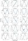 |
Fig. 1. Phase-folded RV curves and orbital solutions constrained by Banyard et al. (2022) for the SB1s. The five marked with (*) do not pass the Lucy-Sweeney test (e/σe ≤ 2.49) and so are consistent with being circular (we show the eccentric solution). The ephemerises used to phase the RV curves are calculated with the orbital solutions in Table 2, with phase 0 corresponding to the periastron passage. |
Orbital solutions for confirmed SB1 systems from Banyard et al. (2022).
For this purpose, we apply the Fourier spectral disentangling in a similar manner as to what was done by Mahy et al. (2022) and Shenar et al. (2022a,b), where the method was used to characterise unseen companions in Galactic and LMC O-type SB1s. The orbital parameters are used as input into finding a self-consistent solution from a time-series of composite spectra obtained for each target, and this optimisation is done with a Nelder & Mead simplex (Nelder & Mead 1965) to find the best solution in a multidimensional space.
There will be a lower limit on the mass of an extracted companion in this disentangling process, and we will be unable to extract the spectral signatures of companions fainter than a certain fraction of the brightness of the primary. This should, by the nature of the primary masses in our sample, be lower than for the systems in the Mahy et al. (2022) study, where the lower limit of unseen companions extracted is about 4–5 M⊙.
After applying spectral disentangling, we now have three categories in which we can place the targets that were identified as SB1s in Paper I. We have those that were found to have a signature of a secondary companion, and as such are newly identified SB2s. These are seven of the 15 targets – NGC 6231 723, HD 326328, CD−41 11030, NGC 6231 78, V*V1208 Sco, CPD−41 7722, and CPD−41 7746. As we identified lower-mass stellar companions in these systems, we discard the possibility of them harbouring a compact object as a companion.
For the remaining eight objects, we tried further to isolate the spectroscopic signature of a putative companion. Since the multidimensional disentangling fit fails to recover the secondary signal, we fixed the orbital period (P), eccentricity (e), longitude of the periastron passage (ω), the time of reference (T0), and the RV semi-amplitude K1 of the primary star, only allowing to K2 to vary. This grid-based disentangling approach (Fabry et al. 2021) is similar to that successfully applied to detect spectral signatures of faint companions with optical brightness contributions below 1% (Shenar et al. 2020; Bodensteiner et al. 2020). While we were able to extract the spectra of the putative companions and characterise their main features, retrieving their semi-amplitude K2 with accuracy was more challenging – typical uncertainties on the values of K2 tended to be around 50 km s−1. This, however, does not impact extracting the spectrum of the companions.
A second category of targets are those that we classified as ambiguous cases, meaning that a secondary object was extracted from the composite spectra, but further attention or data is required to allow their characterisation. For example. the extracted spectra of a secondary companion may not resemble a stellar spectrum, or we might detect Balmer lines in the spectrum without being able to characterise the companion. This could be due to the potential companion being too faint for the limits of this methodology. From the second category, there are 4 targets – V* V946 Sco, CD−41 11038, CXOU J165421.3-415536, and NGC 6231 225. Finally, the third category are targets where no companion could be identified through spectral disentangling, of which there are 4 – HD 152200, CPD−41 7717, NGC 6231 255, and NGC 6231 271. In these cases, the output spectra appear featureless.
As a result, we subject targets in these latter two categories (both the ambiguous cases, and those which we have not been able to identify as SB2s) to more rigorous study to see whether the possibility of a compact object companion can be discounted.
We performed extensive simulations to determine the sensitivity of the spectral disentangling. The goal of these simulations is to be able to exclude the presence of a non-degenerate companion down to certain mass and certain flux ratios. For our simulations, we started with considering binary systems where the properties are similar to those of our visible stars (see Table 3). Given that the masses of the visible stars are just an indication to compute the mass ratio with the mock object, we consider the average estimate between the spectroscopic and the evolutionary masses. To build the mock composite spectra, we use the observed composite spectra and we inject a synthetic spectrum (with a matched S/N to the observations) with the characteristics of the mock objects, scaled by the flux ratios, and shifted by the appropriate radial velocities. We assume a fixed v sin, i of 150 km s−1 for the simulations, which is half the expected critical rotation for a 1.7–2.3 M⊙ star. TLUSTY (Hubeny & Lanz 1995) model spectra is used for simulations above 15 000 K, whereas below 15 000 K, POLLUX models (Palacios et al. 2010) are used. To estimate the properties of the mock stars (spectral types, effective temperatures, masses, and absolute visual magnitudes), we use the tables from Schmidt-Kaler (1982). The stars listed in Table 3 are all classified as B0V or B2V. The absolute V-band magnitude of a B0V star is predicted to MV = −4.0, while that of a B2V star is MV = −2.45.
For the B0V primaries, we were able to extract the spectrum of the secondary object down to a spectral type B9V or A0V, i.e. objects with flux ratios of about 1%–1.5% and mass ratios of about 0.10–0.15. This corresponds to secondaries with absolute V magnitude of MV = 0.2 − 0.65 and masses of roughly 2.3–2.5 M⊙. When the primaries are classified as B2V, we managed to extract the mock spectra of the secondaries down to spectral types A5V or A7V, i.e., objects with mass and flux ratios of about 0.02 and 0.015, respectively. This corresponds to absolute V magnitude of MV = 1.95 − 2.2 and masses between 1.4 and 2.0 M⊙ (Fig. 2).
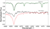 |
Fig. 2. Results from simulated spectra of a mock B2V + A7V binary mimicking the real orbit and data of CPD −41 7717. In green and in red, the synthetic spectra (templates) computed from the stellar parameters of the primary and the secondary components, respectively. The spectra of the secondary have been shifted vertically for clarity. |
We also consider the possibility that the non-detected companions could be stripped stars. We adopted the parameters given by and models produced by Götberg et al. (2018) at solar metallicity. When the visible primary star is classified as B0V, our observed data would be of sufficient quality to extract a stripped star companion with a temperature Teff = 62 kK and a radius of R ∼ 0.55 R⊙, i.e., an object with an initial mass of about Mini ∼ 8.5 M⊙ and a stripped mass of Mstrip ∼ 2 M⊙. When the visible primary star is classified as B2V, we can extract the spectrum of a stripped star down to an Teff = 43 kK and a radius of R ∼ 0.34 R⊙, i.e., an object with an initial mass of about Mini ∼ 4.5 M⊙ and a stripped mass of about Mstrip ∼ 1 M⊙. It should be noted that stripped stars of Mi = 4.5 M⊙ form the earliest after 100 Myr, and so NGC 6231 should not contain such objects.
Another possibility is that the B star component can be spun up due to mass transfer from a stripped star component. In this case, due to the rotational broadening of the spectral component of the B star, it would be the stripped star that would dominate the composite spectrum. However, as none of the spectra resemble stripped star spectra, we can discard this.
The last case that we considered for the is the case of a triple system, with two tight low-mass stars forming the inner system and the B-type stars orbiting around with a wider orbital period. While it is difficult for HD 152200 and CPD −41 7717 to be considered as triple systems given their short orbital period, the three other objects listed in Table 3 have all orbital period longer than 80 days. According to Toonen et al. (2020; based on the stability criterion described by Mardling & Aarseth 1999, 2001), a triple system, composed of an inner system with two A7V stars or later and an outer B-type star orbiting with the parameters given in Table 2, would be considered as stable. If the two inner stars are earlier than A7V, the triple system would be unstable. We also consider the light ratios involved in such systems, where the two stars in the inner system have a similar light contribution, and then we compare with the B star in the outer system. Each low-mass star would contribute between 0.3 and 1.2% to the total flux (depending whether we consider a B0V primary or a B2V). Therefore, F stars in an inner close system would be extremely difficult to detect, but late A-type stars would be detectable. However, the resolution of our composite spectra would not be sufficient to extract the individual contribution of the low-mass stars, but rather a merged spectrum.
3.2. Atmosphere modelling
To constrain the mass of the unseen secondary using the binary mass function (Sect. 3.4), we first need an estimate of the primary mass. We choose to do this in two ways – by estimating the spectroscopic mass of the primary star, and by estimating the evolutionary mass of the primary star. The spectroscopic mass is named as such as it is computed with stellar gravities and radii (Mspec ∝ gR2) determined through the fitting of stellar spectra and SEDs. The evolutionary mass, on the other hand, is inferred by comparing the target’s properties, namely log(L/L⊙), Teff, log g, and v sin i, to stellar evolutionary tracks.
For both of these estimates, we first need to estimate the stellar parameters of the primary star. Specifically, we want to obtain the effective temperature (Teff), the surface gravity (g), the projected rotational velocity (v sin i), the stellar radius (R*), and the bolometric luminosity (Lbol) of the primary star, along with the extinction to the star, expressed in this Section as the colour excess, E(B − V). We use cgs units unless indicated otherwise.
We can obtain estimates to these parameters by adopting a grid-oriented fitting approach, based on synthetic TLUSTY (Hubeny & Lanz 1995) models that relax the assumption of local thermodynamic equilibrium (non-LTE or NLTE), and following the implementation developed by Bodensteiner et al. (2023).
3.2.1. Spectroscopic fitting
In this implementation, we first combined all the observed composite spectra of an SB1 after having shifted them with their RVs (measured in Paper I) to put them in the same reference frame, and then we have co-added them to produce a master spectrum of the primary star with a higher signal-to-noise ratio (S/N) than in the individual epochs. We then fitted these master spectra with a TLUSTY model degraded to the resolution of our observed spectra (λ/δλ ∼ 6500) and rebinned to the wavelength step of our data. We use both the BSTAR2006 (Lanz & Hubeny 2007) and OSTAR2002 (Lanz & Hubeny 2003) grids to include the hottest stars in our sample. The BSTAR2006 grid contains synthetic spectra for effective temperatures from 15 000 to 30 000 K in steps of 1000 K, and log g from 1.75 to 4.75 with 0.25 dex steps. The OSTAR2002 grid’s synthetic spectra have effective temperatures ranging from 27 500 K to 55 000K with steps of 2500 K (we truncate the grid here to 30 000 K as effective temperatures below this are already present in the BSTAR2006 grid with a smaller step), and log g from 3.0 to 4.75 in 0.25 dex steps. Both grids have solar metallicities. The BSTAR2006 grid spectra have a microturbulence of 2 km s−1, whereas those in OSTAR2002 have a microturbulence of 10 km s−1. Spectra in both grids have a coverage of the entire UV to optical range (900–10 000 Å).
The spectroscopic fitting allows us to constrain Teff, log g, and v sin i from each target’s master spectrum. To account for v sin i, we pre-broaden each TLUSTY model with a range of v sin i values from 20 to 400 km s−1. The best-fitting model is then constrained by locating the minimum of the χ2-distribution for each of the three parameters. 1-σ errors are calculated from the estimated 68.2 % confidence interval on the parameter range.
We run into the limitations of using the TLUSTY grid when we consider the targets in our sample that have effective temperatures below 15 000 K (i.e. are later than spectral type B5), of which there are three (NGC 6231 255, NGC 6231 273, and NGC 6231 225, all classified as B9 stars). For these stars, GSSP (Tkachenko 2015) or other databases of synthetic models matching low-mass star properties such as, for example, Kurucz (1979), ATLAS9 (Castelli & Kurucz 2003), or PHOENIX (Allard 2016), should be used for constraining their stellar parameters. However, based on the expected mass of a B9 star and the very small binary mass functions of these SB1s (Table 2), we do not consider these as likely candidates for harbouring compact objects, and so we exclude them from further study in this work. This reduces the sample of potential candidate systems in this work to five. However, finding such a low-mass BH binary would be a potential progenitor of known low-mass BH X-ray binaries, and so such a find would be interesting.
3.2.2. Photometric fitting
Alongside the spectroscopic fitting, similar to the original implementation by Bodensteiner et al. (2023), we also fit the synthetic spectral energy distributions (SEDs) provided for each TLUSTY grid to observed photometry of various catalogues (Table 1). The photometry we used is chosen to cover the ultra-violet (UV) to the near-infrared (NIR) domain of the SED of each B star. As described in Sect. 2.2, the magnitudes and their associated uncertainties in the J, H, and Ks bands are retrieved from 2MASS (Skrutskie et al. 2006), those in the U, V, B and I bands were obtained by Sung et al. (2013), and G, GBp, GRp magnitudes were retrieved from Gaia eDR3 (Gaia Collaboration 2016, 2021).
We use the same grid-search approach as the spectroscopic fit, where our best-fitting model is constrained through locating the minimum of the χ2-distribution of several parameters. The same parameter spaces are explored as described in Sect. 3.2.1 for Teff and log g. The constraints on Teff and (especially) log g are weaker here than for the spectroscopic fits, but the advantage of using the photometric fit is in constraining the stellar radius, and therefore the luminosity, of the target. For the photometric fit, we scale the TLUSTY model grid to stellar radii from 3 to 12 R⊙ in steps of 0.1 R⊙, and colour excesses from 0 to 0.9 mag in steps of 0.1 mag. To implement these further two parameter ranges in the grid, for every model in the grid of Teff and log g we scaled the flux at the stellar surface with the distance to NGC 6231 (1.71 kpc, Kuhn et al. 2019) and then to each stellar radius in the radius grid. Then, interstellar exctinction is applied to every model through the python package DUST EXTINCTION2 in the colour excess range defined above. This gives us a 4-dimensional grid of SED models to fit the observed photometry with observed photometry of various catalogues.
3.2.3. Combined fit
To find the best-fitting model for all the parameters explored between the spectroscopic and photometric fitting, and again in a similar manner to Bodensteiner et al. (2023) we combine the computed χ2 from each independent fit of each model with common values of Teff and log g, but varying values of v sin i, radius, and colour excess. The result is a 5-dimensional grid, with the parameters of Teff, log g, v sin i, radius, and colour excess. The constrained stellar parameters for the SB1 candidates identified in Sect. 3.1 are presented in Table 3. The spectroscopic mass estimates provided in Table 3 are calculated from the gravities and radii constrained for each star from the combined fit.
3.3. Evolutionary fitting
Now that we have constrained the stellar parameters of the primary stars of our sample, we can provide a second estimate of the primary mass through evolutionary fitting. We use the obtained log(L/L⊙), Teff, log g, and v sin i as input for the code BONNSAI (BONN Stellar Astrophysics Interface, Schneider et al. 2014, 2017), which uses Bayesian statistics to compare observed stellar parameters to evolutionary stellar models, and provides predicted evolutionary parameters for the targets, including the evolutionary mass and the age of the star. It should be noted that these estimates will only be consistent with systems that have not interacted before. In this work, we compare our inputted parameters against the BONN single-star evolutionary models of Galactic metallicity (Brott et al. 2011). The predicted evolutionary masses and ages are presented in Table 3.
There is a potential mass discrepancy present between the spectroscopic and evolutionary estimates of the primary masses of these stars (Fig. 3) at higher masses, though the large errors on the spectroscopic masses of HD 152200 (and to an extent, CD−41 11038) make this unclear. The discrepancy in the estimation of stellar masses has long been an issue (Herrero et al. 1992; Burkholder et al. 1997; Weidner & Vink 2010; Mahy et al. 2020). The mass discrepancy found in intermediate- and high-mass eclipsing SB2 stars has been discussed by Tkachenko et al. (2020), where it was concluded that the discrepancy was a result of an under-estimation of the convective core mass of these stars and the neglect of high micro-turbulent velocities and high turbulent pressure in stellar atmosphere models in the spectral analysis of these stars. However, robustly studying the mass discrepancy in our own targets is out of the scope of this work, and so we consider both estimates of the primary mass going forward.
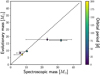 |
Fig. 3. Comparison of the spectroscopic and evolutionary estimates of the compact object candidate SB1s, along with their orbital periods. The dashed line indicates agreement between the two estimates. |
There is also a discrepancy between the estimated age of NGC 6231 and the ages of some of the SB1s. Ages for the cluster have been derived between 2 (Sana et al. 2006, 2007) and 7 (Sung et al. 2013) Myr. However, V* V926 Sco, CXOU J165421.3-415536 and CPD−41 7717 all have evolutionary age estimates above this range. This is especially true in the case of CPD−41 7717, which has an estimated evolutionary age of  Myr. Accretion from a donor and consequential rejuvenation effects would result in the star appearing younger than expected, but it becomes more difficult to explain stars that appear older than expected. This could be a signature of more continuous star formation in the cluster.
3.4. Minimum masses of unseen companions
With the estimated primary masses (both spectroscopic and evolutionary) obtained, the ranges of masses of the unseen companions can be calculated in the same manner as Mahy et al. (2022). We compute the minimum companion mass for the SB1 systems for which no signature of a companion has been extracted with the spectral disentangling. For that purpose, we use the binary mass function f(m), and the spectroscopic and evolutionary masses (estimated in Sects. 3.2 and 3.3 respectively) of the primary stars:
where Mu is the mass of the unseen companion, Mp the mass of the primary star, i the inclination, Porb the orbital period of the binary system, e the eccentricity of the orbit, K the RV semi-amplitude of the primary star, and G the gravitational constant. As sin i lies between 0 and 1, we can write f(m) as an inequality:
and so we can now solve this inequality to get two estimates of the minimum mass of the unseen companion, one with the spectroscopic estimate for the primary mass and one with the evolutionary estimate of the primary mass.
We can also independently constrain the lower limit of the inclination, i of each system. To do this, we estimate each primary star’s critical rotational velocity, vcrit, which we define as:
where G is the gravitational constant, Mp the mass of the primary star, and Rp the radius of the primary star. Without information on the inclinations of the systems in our sample, we make the assumption that the stellar radii, Rp that we constrain through our analysis are equal to the polar radii of the stars. We also make the assumption that the rotational axes are perpendicular to the orbital plane, and that the maximum rotational velocity of the star is the computed critical velocity (Eq. (3)), then it follows that

From this we can constrain a minimum inclination for each binary system, and consequently a maximum mass of the unseen companion of each system. This assumption does not hold for systems that have NS companions (and potentially those with BH companions) due to the misalignment of the rotational and orbital axes due to a supernova kick. This impacts only the upper limit on the predicted mass of the unseen companion, and so does not impact our conclusions.
We use Eqs. (2) and (4), which rely exclusively on the constrained orbital parameters (Paper I) and stellar parameters (Sect. 3.2), to compute the possible range of masses of the unseen companions of the candidate systems identified in Sect. 3.1. Figure 4 shows the relation between the inclination of the systems and the mass of the unseen companion using the spectroscopic estimate of the primary masses, and Fig. 5 shows the same, but calculated with the evolutionary estimate of the primary masses.
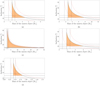 |
Fig. 4. Computed mass of the unseen companion of the SB1s as a function of the inclination of the system using Eqs. (2) and (4), and using the spectroscopic estimate of the primary mass. The minimum inclination of each system is indicated by the horizontal line, with the associated error as dashed horizontal lines. The vertical line indicates the minimum mass of the unseen companions, with the associated error as dashed vertical lines. The orange shaded regions correspond to the possible values for the system inclinations and the masses of the unseen objects. The red dashed line corresponds to the uncertainty on the binary mass function, computed by propagating the 1σ errors on the other parameters. (a) HD 152200, (b) V* V946 Sco, (c) CD–41 11038, (d) CXOU J165241.3-415536, (e) CPD–41 7717. |
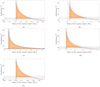 |
Fig. 5. Same as Fig. 4, but using the evolutionary estimate of the primary mass. (a) HD 152200, (b) V* V946 Sco, (c) CD–41 11038, (d) CXOU J165241.3-415536, (e) CPD–41 7717. |
3.5. TESS photometry
Another tool at our disposal in detecting lower mass stellar companions to the SB1s is photometry. For example, if one of these systems is found to be an eclipsing binary (EB), then logically the presence of a stellar companion is inferred. However, there are also signatures of detached (and thus quiet, non-interacting) stellar BHs that can be found in space-based photometry as obtained by, for example, TESS. Masuda & Hotokezaka (2019) have illustrated multiple potential periodic signals from the visible component in TESS light curves (LCs). Ellipsoidal variations occur as a result of tidal distortion of the primary star due to the gravity of the BH (and due to non-BH companions), causing the geometric shape and the brightness distribution of the visible star to change. Doppler beaming results in an amplitude variation of the light curve caused by the relativistic aberration of the visible star’s light, time dilation, and the Doppler motion of the visible star’s light. These two effects are dependent on and are in phase with the orbital period of the binary system. The third signature then, is self-lensing: this occurs when the BH eclipses the visible star, and the BH acts as a lens, gravitationally magnifying the star. It is, however, unlikely to find any indication in the light curve of the presence of a non-degenerate companion in systems with longer orbital periods.
The retrieval and reduction of the TESS lightcurves is described in Sect. 2.2.2. The light curves were observed in the TESS sector 39. We display in Fig. 6 the light curves and their periodograms. These periodograms were computed using the Heck-Manfroid-Mersch technique (Heck et al. 1985; revised by Gosset et al. 2001). Because the field is very crowded, the extraction of the TESS light curves was challenging (see Sect. 2.2.2). We were not able to extract the TESS light curves for 6 objects in our SB1 sample: CD −41 11030, CD −41 11038, NGC 6231 78, NGC 6231 255, NGC 6231 273, and NGC 6231 225. All these objects suffer from contamination from other stars in their neighbourhood.
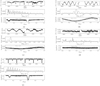 |
Fig. 6. TESS light curves, their periodograms, and the light curves phased with the best found period, of five of the targets in which we detected photometric variability. (a) V* V1208 Sco, (b) CPD–41 7717, (c) HD 152200, (d) CXOU J165421.3-415536, (e) CPD–41 7746. |
We found two systems showing eclipses in their light curves: V* V1208 Sco, and CPD−41 7746. These systems were already detected as SB2 after applying spectral disentangling (see Sect. 3.1). Two other objects show photometric variability: HD 152200, and CPD−41 7717. We were not able to extract the spectra of the companions in these two objects after the spectral disentangling. The signals in these light curves have the same period as their orbital ones. This excludes ellipsoidal variations or eclipses as possible cause, where the signal would have had half the orbital periods. Given the projected rotational velocities, the estimated radii of the visible stars, and the detected periods, it is unlikely that these signals can come from rotation. Finally, the light curve of CXOU∼J165421.3−415536 has a significant frequency that corresponds to a period of 0.6967 days. If this signal is due to the rotation, that implies that the inclination of the star (and perhaps the system) is about 31°. That inclination, assuming that the rotational axes are perpendicular to the orbital plane, would give a mass of about 1.8 M⊙ for the unseen companion. However, we do not exclude that the light curve of CXOU J165421.3−415536 might be affected by contamination from other close-by objects.
Previous photometric studies on some of the stars in our sample do not indicate any of the above signatures of BHs, but there are findings of note. Meingast et al. (2013) performed a study with Johnson UBV photometry to identify pulsating and otherwise variable stars in NGC 6231. Out of the initial 15 stars described in this work (both SB1s and newly double-lined SB2s), HD 326328 was found to be an slowly pulsating B-star (SPB) candidate, NGC 6231 225 was classified as an SPB, and V* V946 Sco was classified as a β Cepheid star. Out of these three, only V* V946 Sco has been found to be a potential candidate for having a compact companion in this work. Otherwise, the only other star in the sample studied photometrically is HD 152200. Pozo Nuñez et al. (2019), in a survey for high-mass eclipsing binaries in Sloan r and i photometry, found HD 152200 to be an eclipsing binary with a period of P = 8.89365 ± 0.00081 days. This is almost exactly twice the orbital period found in Paper I for this system, which was P = 4.4440 ± 0.0007 days. It should be noted that the authors were unable to model the Roche geometry of the system using the obtained LC. If this system is indeed an EB, then this is not compatible with the proposal that the unseen companion is a compact object and also not compatible with the derived RVs of the visible star. The period is compatible with that of a slowly pulsating B-type star, however, the star’s LC does not appear to indicate that the variability is solely due to pulsations.
4. Discussion
4.1. Newly identified SB2 systems
We found seven of the 15 previously identified SB1 B-type binaries of NGC 6231 to be SB2s through Fourier disentangling (Sect. 3.1), where the signature of a secondary star has been extracted from the composite spectrum. These targets are NGC 6231 723, HD 326328, CD−41 11030, NGC 6231 78, V*V1208 Sco, CPD−41 7722, and CPD−41 7746 (see Fig. A.2 for the disentangled spectra). We have been able to probe down to a mass ratio of near 0.1, which is significantly lower than what was found in Paper I. Figure 7 shows the mass ratio distribution of the NGC 6231 B-type SB2s, along with the detection probability curve computed for the observational campaign to account for the observational biases. The original campaign had a significant drop in sensitivity to objects with a mass-ratio below 0.4, and as was proposed in Paper I, most of the missing low mass ratio systems have been found in the originally proposed ‘SB1s’.
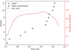 |
Fig. 7. Observed cumulative mass-ratio distribution of the SB2 stars in NGC 6231, with the Paper I SB2s as crosses, and the newly disentangled SB2s as stars. The detection probability, calculated from the bias correction of the observational campaign in Paper I, is displayed as a red curve. |
Figure 8 shows the orbital periods against the eccentricities of the newly disentangled systems, alongside the SB1s and the SB2s identified visually in Paper I. Most of these SB2 systems seem to have periods around 30 days, and this was previously noted as a feature in the full period distribution (SB1s and SB2s) in Paper I, and could not be explained by alliasing of the frequency space of the observational campaign by, for example, its cadence. We also found the new SB2s to have eccentricities from effectively circular up to around 0.5.
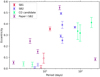 |
Fig. 8. Orbital period against eccentricity of the B-type binaries in NGC 6231. The SB1s are shown in red, with the candidates for harbouring compact objects in green, the Fourier disentangled SB2s in blue, and the SB2s identified in Paper I in purple. Open faced symbols indicate systems that have eccentricities that do not pass the Lucy-Sweeney test (e/σe ≤ 2.49) and so are consistent with being circular. |
4.2. Candidates for harbouring compact objects
The remaining eight targets, then, are those that we cannot extract a companion’s signature through Fourier disentangling of their spectra. As stated in Sect. 3.2.1, three of these have primary stars of spectral type B9 and very small binary mass functions, and so we exclude them from the candidates for harbouring compact objects. This leaves a remaining five SB1 systems. Figure 9 shows both the estimated spectroscopic and evolutionary estimates of each system’s unseen companion, as calculated with the binary mass function (Eq. (2)) with the estimated spectroscopic (Sect. 3.2) and evolutionary masses (Sect. 3.3). Also shown in Fig. 9 is the predicted mass range for Galactic stellar BHs and NSs (Belczynski et al. 2010; Fryer et al. 2014). For the NSs, this is between 1.2–2.5 M⊙, and for BHs this is above 5 M⊙. The estimated masses of the unseen secondary and the detection limits of the spectral disentangling are detailed for each target in Table 4.
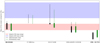 |
Fig. 9. Estimated spectroscopic (black) and evolutionary (green) masses of each SB1’s unseen companion. The blue zone corresponds to the predicted mass range for Galactic stellar mass BHs and the red zone represents the same but for Galactic NSs (Belczynski et al. 2010; Fryer et al. 2014). The mass ranges for each target where main sequence stars cannot be discounted according to the spectral disentangling sensitivity (Sect. 3.1) are denoted by thick lines. Target names in boldface are the targets for which no companion could be extracted through spectral disentangling, and the other targets are those for which the nature of the extracted companion was ambiguous (Sect. 3.1). |
Estimated masses of the unseen secondaries of the five SB1s.
4.2.1. HD 152200
HD 152200 was spectrally classified as a B0V star with a 4.44 d orbital period with circular eccentricity in Paper I. In this work, the star’s spectroscopic mass was constrained to be 23.4  , and the evolutionary mass constrained was 17.8
  . Using the binary mass function, and the constrained primary mass estimates and the orbital parameters of the system, the range of possible masses for the companion of HD 152200 is between 1.1 and 3.5 M⊙ (analogous to a late F to a B8 MS star).
During disentangling, this star was classified as a target from which we could not unambiguously extract a companion from the spectra. According to the simulations described in Sect. 3.1, which were designed to reject the presence of non-degenerate companions down to certain mass and flux ratios, it was found that, considering a B0V primary, we are able to extract the spectrum of a secondary object down to a spectral type of B9V or A0V. We can likely reject the possibility of a hidden non-degenerate MS companion above 2.2 M⊙, but this does not discount the entire range of possible masses for HD 152200’s companion, for which the minimum is 1.1 M⊙. When considering a stripped star companion, we can expect to be able to extract a stripped star companion with a temperature Teff = 62 kK and a radius of R ∼ 0.55 R⊙, i.e., an object with an initial mass of about Mini ∼ 8.5 M⊙ and a current stripped mass of Mstrip ∼ 2 M⊙. As we have limited information due to the limited wavelength coverage of our composite spectrum, we are missing access to signatures of a stripped star companion, so this does increase the difficulty in detecting these stars. One of these, for example, is strong He IIλ4686 emission. The wavelength region we have access to, 3964–4567Å, mostly consists of weak absorption lines. However, the most massive stripped stars in the Götberg et al. (2018) models, i.e. the WN3 stars (those with Mini > 15 M⊙), have strong emission features in the wavelength domain we are observing, and so it is likely we can exclude these. It is important to note, however, that the strengths of the line depend on the assumed wind mass loss rates which are uncertain for stripped stars. As for the possibility of being a triple system, it would be unlikely due to HD 152200’s short period. Based on the prediction of the unseen masses, if the companion was a compact object, it would likely be a neutron star.
Regarding the light curves of HD 152200, the target remains an ambiguous case with reports of the star being an eclipsing binary with a period of twice that found in Paper I (P = 8.89365 ± 0.00081 d, Pozo Nuñez et al. 2019). While there is definitely photometric variability, there do not appear to be eclipses in the TESS photometry (see Fig. 6). As mentioned in Sect. 3.5, as the variability appears to have the same period as the orbital period constrained in Paper I, this excludes ellipsoidal variations (due to a close compact object companion, for example) or eclipses, as these would have half the orbital period. This remains an interesting object that would benefit from further photometric study.
The stellar content of NGC 6231 has been subject to multiple X-ray surveys in the past. An XMM-Newton campaign towards NGC 6231 was performed by Sana et al. (2006), and Chandra observations were obtained by Damiani et al. (2016) for the stars of NGC 6231. HD 152200 appears across the XMM-Newton and Chandra surveys, and the surveys find HD 152200 to have an X-ray luminosity of log LX = 31.29 and log LX = 31.32, respectively. Given the early-type nature of these stars, this value is not unexpected and does not suggest active accretion from a compact object. Along with this, HD 152200 (and the rest of the CO candidates) are not detected in the Second ROSAT all-sky survey (Boller et al. 2016). This suggests the potential compact objects in these binary systems are X-ray quiet (dormant), but does not disqualify these companions from being lower-mass MS stars.
4.2.2. V* V946 Sco
V* V946 Sco was found to be a B2V star with a 97.9 d orbit in Paper I. The star’s spectroscopic and evolutionary masses were constrained to be 10.4 and 9.4
 , respectively. The companion to V* V946 Sco, then, is estimated to be between 2.5 to 7.8 M⊙ when taking both the spectroscopic and evolutionary primary mass estimates into account, which would be classified between B9 and B2.
The disentangling status of this star was that the nature of the extracted companion was ambiguous. The detection limits we found for B2V stars were MS companions of spectral type down to A5V or A7V, corresponding to masses of 1.4 and 2.0 M⊙. This means that if V* V946 Sco’s companion was a MS star, we should be able to extract it from the spectra. If the companion was a stripped star, for a B2V primary star, we can extract the spectrum of a stripped star down to Teff = 43 kK and a radius of R ∼ 0.34 R⊙, i.e., an object with an initial mass of about Mini ∼ 4.5 M⊙ and a current stripped mass of Mstrip ∼ 1 M⊙. Another case that was considered was a triple system, with two tight, low-mass stars forming the inner system and the B-type star in a wider orbit. The contribution of two F stars in the inner system, which would contain a total mass of ∼2 − 3 M⊙, would be very difficult to extract, and so this remains a possibility as this is within the range of possible masses for the companion of V* V946. However, two late-A stars in the inner system, with a combined mass of ∼3.5 M⊙, should be detectable, and so we can exclude systems of these masses. If the two stars are any earlier than A7V, the system would likely become unstable.
As V* V946 Sco has a relatively long orbital period compared to the duration of a sector of TESS, it is not likely to have an indication in its light curve of the presence of a non-degenerate companion with TESS. It’s orbital period is, however, close to the peak of predicted period distribution of OB+BH binaries, and also close to the peak of the observed orbital period distribution of Galactic Be/X-ray binaries (Langer et al. 2020). This also applies to the targets CD−41 11038 and CXOU J165421.3-415536.
Finally, the X-ray luminosities listed in the XMM-Newton and Chandra surveys are log LX = 30.06 and log LX = 30.87, respectively. Again, these are not unusual for non-accreting early-type stars. However, in these longer period cases, the low X-ray luminosity does not discount wind accretion by a potential compact object companion, as in a 100 d orbit, wind accretion does not result in detectable X-ray emission (Mahy et al. 2022). Overall, as we can likely rule out both MS and stripped companions for this object, V* V946 Sco is a strong candidate for harbouring a compact object.
4.2.3. CD−41 11038
CD−41 11038 was classified as a B0V star with a 83.9 d period. The spectroscopic and evolutionary masses constrained for the object are 32.1  and 17.2
  respectively. It should be noted that the spectroscopic estimate of the mass far exceeds the mass expected of a B0V star, and corresponds more closely to that of a 07V/08V star. In Paper I, these stars were classified with the criteria in (Evans et al. 2015), where the earliest classification for B-type dwarfs was B0V. Following these mass estimations, CD−41 11038 is estimated to have a companion of a mass between 1.6 and 26 M⊙, and would be classified as a late-A/early-F star up to around spectral type O8, and also enters the predicted mass range for Galactic stellar BHs.
CD−41 11038 is another target for which the nature of the extracted companion was ambiguous. Again, like HD 152200 (also a B0V) star, we can expect to be able to extract MS companions down to spectral type A0V, meaning that we should be able to discount any MS companions above 2.2 M⊙. However, the minimum possible mass of the unseen companion does undercut this slightly, so it is possible that an early-F/late-A star is present, yet hidden. If we consider a stripped companion, like HD 152200, we should be able to extract one with an initial mass of Mini ∼ 8.5 M⊙ and a current stripped mass of Mstrip ∼ 2 M⊙. As for the case of CD−41 11038 being in a triple system, we again cannot discount an inner binary system consisting of F-type stars, but we can exclude late A- and earlier-type inner systems as they would either be detected or dynamically unstable.
CD−41 11038’s TESS lightcurve is unfortunately contaminated with light from neighbouring stars, so no information is able to be gleaned from it. However, it does also have a relatively long period compared to the duration of a TESS sector, and so is unlikely to show an indication in its light curve of the presence of a non-degenerate companion, as it would be unlikely that an eclipse would be observed.
The X-ray luminosities for the star found by the XMM-Newton and Chandra surveys are log LX = 31.78 and log LX = 31.57 respectively. This is again typical for non-accreting early-type stars, but the same wind accretion possibility as for V* V946 Sco applies here. CD−41 11038’s high predicted unseen companion masses make it a strong candidate for harbouring a BH.
4.2.4. CXOU J165421.3-415536
CXOU J165421.3-415536 was classified as a B2V star in Paper I, with a 204 d period constrained for the SB1 system. The spectroscopic and evolutionary masses constrained for this target are 7.3  and 7.0
  respectively. Consequently, the range of masses of the unseen companion is predicted to be between 0.9 and 3.1 M⊙, which corresponds to a late-G to a B8 main sequence star.
The nature of CXOU J165421.3-415536’s spectrally disentangled companion was also found to be ambiguous. As CXOU J165421.3-415536 is a B2V star, according to our detection limit simulations, we should be able to extract the spectra of MS companions of spectral types down to A5V or A7V, corresponding to masses of 1.4 and 2.0 M⊙, which does mean that there is potentially a solar-like or even sub-solar mass MS companion to CXOU J165421.3-415536 that we do not detect. As for a stripped star companion, we can expect to extract the spectrum of a stripped star down to an Teff = 43 kK and a radius of R ∼ 0.34 R⊙, i.e., an object with an initial mass of about Mini ∼ 4.5 M⊙ and a current stripped mass of Mstrip ∼ 1 M⊙. As for the triple system case, we again cannot discount an inner system consisting of two F stars, though we can disqualify late A- and earlier-type systems due to both being able to detect them and also to the instability of the earlier-type systems.
The Chandra survey provides an X-ray luminosity of log LX = 31.78 and log LX = 30.16, and which is again typical for quiescent early-type stars, but again we cannot discount the possibility of wind accretion from a compact object due to the system’s relatively long orbital period.
4.2.5. CPD−41 7717
CPD−41 7717 was classified as a B2V star in Paper I with an orbital period of 2.5 d. Spectral disentangling of CPD−41 7717 did not result in the extraction of the signal of a companion. The spectroscopic and evolutionary masses constrained for the star are 6.1 and 8.2
 . The resulting range of possible unseen companion masses, 0.4–1.2 M⊙, is below the predicted mass range for Galactic NSs, and it is likely that a solar-like companion is hidden in the composite spectrum. This mass range is also beneath the estimated detection limit for MS star companions, which for B2V stars is down to A5V or A7V stars, corresponding to masses of 1.4–2.0 M⊙, so it is likely that the companion is a low mass MS star, below the detection limits. Regarding a potential stripped star companion, we can expect to extract the spectrum of a stripped star down to an Teff = 43 kK and a radius of R ∼ 0.34 R⊙, i.e., an object with an initial mass of about Mini ∼ 4.5 M⊙ and a current stripped mass of Mstrip ∼ 1 M⊙.
The short orbital period of CPD−41 7717 makes it viable to use TESS to reject a non-degenerate companion through the possibility of detecting an eclipse. CPD−41 7717 does show photometric variability in its LC, however, we do not observe any eclipses. We also find its variability to have the same period as its orbital period.
X-ray luminosities are not provided by either the Chandra and XMM-Newton surveys for CPD−41 7717, so no conclusions can be made on its X-ray output. However, it has been established by the star’s predicted companion masses that it is unlikely that the companion is a compact object, and so even if the system was an interacting one, the system should not be visible in the X-ray spectrum.
4.3. Supersynchronous rotation
Figure 10 shows the constrained v sin i for the visible stars in candidate binaries with a compact object as a function of their orbital period. Also displayed here are the critical rotational velocities calculated for each star using Eq. (3), and using the parameters constrained with both the spectroscopic (and photometric) and evolutionary fitting. It is clear that none of the constrained values of v sin i are close to critical.
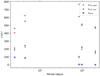 |
Fig. 10. Orbital period against projected rotational velocity, v sin i (in black). Red plusses correspond to the critical rotational velocity, vcrit, calculated with Eq. (3). Blue crosses are the computed synchronous rotation rate, vsync, computed for each star assuming they are in a synchronous orbit. |
However, for the shorter period systems (HD 152200 and CPD−41 7717), the constrained values of v sin i are around a factor of two higher than the theoretical synchronous rotation velocity, vsync. This is assuming the rotational period of the star has tidally synchronised with the orbital period of its binary system, and so is computed with the orbital period of each system and the radius of the visible star. The synchronisation timescale, according to Zahn (1977), is proportional to  , where a is the semi-major axis of the orbit. As a result, only close binary systems are expected to potentially exhibit this behaviour.
To predict the synchronisation timescales of these shorter period systems and ascertain whether these two targets are compatible with them, we can follow what was done by El-Badry et al. (2022) for the proposed BH candidate NGC 2004 #115 in the LMC (Lennon et al. 2022). In that work, they use the Zahn theory, in which the predicted synchronisation timescale is estimated to be
where M and R are the mass and radius of the star undergoing synchronisation, in this case the primary star, q is the mass ratio (q = M2/M), G is the gravitational constant, a is the semi-major axis of the binary, β = I/MR2, where I is the primary star’s moment of inertia, and E2 is the tidal torque coefficient of the primary star. Further modelling of these systems, for example with MESA (Paxton et al. 2011), is required to estimate β and E2. An analytic approximation for E2, obtained by Yoon et al. (2010) from fitting the work of Zahn (1977), is E2 = 10−1.37(Rconv/R)8, where Rconv is the convective core radius. However, alternate analytic approximations for E2, specifically for H-rich and He-rich stars have been formulated by Qin et al. (2018). They are E2 = 10−0.42(Rconv/R)7.5 for H-rich stars, and E2 = 10−0.93(Rconv/R)6.7 for He-rich stars. We consider each approximation for E2 in our predictions of the synchronisation timescales of the two short-period systems.
For CPD−41 7717, we calculated a model for a 5 Myr-old 6.07 M⊙ star using MESA (version 15140). The input physics of the simulations match those used in the Galactic Brott et al. (2011) models. We found that, from this model, β = 0.06, and Rconv/R = 0.2. Taking the average estimate for the unseen companion’s mass from the spectroscopic mass estimate of the primary, we assume M2 = 0.65M⊙. We also assume a = 14R⊙ from the system’s period. If we use the same prescription (Yoon et al. 2010) for E2 used by El-Badry et al. (2022), then we estimate the synchronisation timescale to be around 360 Myr. However, using the Qin et al. (2018) prescriptions lead to a synchronisation timescale of around 15 Myr. Given this, it is unlikely for this system to be synchronised based on the cluster age.
For HD 152200, a 5 Myr-old 23.35 M⊙ MESA model was calculated. We found that, from this model, β = 0.05, and Rconv/R = 0.2. Like for CPD−41 7717, take the average spectroscopic estimate of HD 152200’s unseen companion as the assumed secondary mass, M2 = 2.4 M⊙. We also assume a = 34 R⊙ from the system’s period. Using the Yoon et al. (2010) prescription for E2 results in an estimated synchronisation timescale of around 60 Myr. However, using the Qin et al. (2018) prescriptions lead to a a synchronisation timescale of around 3 Myr, which means that there is a possibility that the system should be synchronised based on what the assumption for the tidal torque coefficient is.
The potential overestimation of v sin i could be due to a few factors. The first is that we do not take the macroturbulent broadening of spectral lines into account during the spectroscopic fitting, as the tool we use does not do this. However, also have relatively low resolution spectra, and so we would have errors of the order of 10 km s−1 in constraining the macroturbelence. The second is that we have relatively low resolution spectra (R ∼ 6500). The third is that we have assumed that the rotation axis of these stars is perpendicular to the orbital plane. If the true v sin i is actually lower for these two close binaries, then the minimum inclination calculated with Eq. (4) will be smaller and as such, the lower bound of the range of unseen companion masses will increase, which decreases the likelihood of the unseen companion being a faint, non-degenerate star.
5. Summary
In this work, we aimed to characterise the unseen companions of the 15 SB1 binary systems that were identified when studying the multiplicity of the B stars in NGC 6231 (in Paper I), using multi-epoch medium-resolution optical spectroscopy, ground-based photometry and high-cadence space-based photometry to do so. Through Fourier disentangling of the spectra, we found 7 SB2 systems with mass ratios down to 0.1, extending past the limits of the original work in Paper I. Out of the other 8 targets, 4 targets were found to be ambiguous cases where the nature of the extracted companion was unclear, and the other 4 targets had no signature of a faint companion in their spectra. Two of targets in the latter category were considered unlikely candidates for harbouring a compact object due to their late spectral type (B9) and their binary mass functions, and so were not considered for further study.
Through atmospheric fitting, which combined both spectroscopic and photometric fitting against a TLUSTY model grid of synthetic spectra and SEDs, we estimated the spectroscopic mass and other stellar parameters of each visible primary star in the remaining SB1s, and then we provided a secondary estimate for the primary star masses through evolutionary fitting with BONNSAI. With these stellar parameters, and using the binary mass function already characterised for each SB1’s orbit in Paper I, we provide two estimates of the unseen companion’s mass for our SB1 systems that we considered candidates for hosting a compact object companion. Consequently, we found four systems (HD 152200, V* V956 Sco, CD−41 11038, and CXOU J165421.3-415536) that have estimated companion masses that fall in the predicted mass ranges for Galactic compact objects. CD−41 11038 and V* V946 Sco are particularly strong candidates for harbouring a compact object companion. However, the detection limits of our methodology do mean that it is possible for some or all of these candidates to have lower mass MS companions, stripped star companions or be part of triple systems.
We also looked at high-cadence TESS photometry to search for signatures of compact object companions in the light curves of these targets. However, as the field around these targets is very crowded, light curve extraction is challenging and we were unable to extract light curves for 6 out of the original 15 targets. Two of the targets showed eclipses in their light curve (V* V1208 and CPD−41 7746), and these two targets were confirmed to be newly disentangled SB2s. Three of the compact object hosting candidates have photometric variability in their lightcurves, though the origin of this variability is uncertain, and their periodicities do not appear to be consistent with signatures of compact object companions such as ellipsoidal variability and eclipsing.
We also find that the two close binaries out of the SB1s, HD 152200 and CPD−41 7717, appear to rotate supersynchronously, i.e. rotate above the speed at which the star would rotate if it was tidally synchronised with its companion. We estimated the tidal synchronisation timescales using Zahn (1977) theory and MESA models, and we find that while it is not expected for CPD−41 7717 to be synchronised given the age of the cluster, it could be expected for HD 152200 to be.
The results presented in this work present four candidate SB1 systems for harbouring compact objects. Further photometric and interferometric follow-up on these candidates will help unambiguously characterise these systems, and consequently will potentially allow us to reduce the uncertainty in compact object formation scenarios. This work also presents a look at the more extreme end of the mass ratio distribution of these B-type stars, which is important input into the synthesis of populations of binary stars and studies of binary star formation.
Acknowledgments
The research leading to these results has received funding from the European Research Council (ERC) under the European Union’s Horizon 2020 research and innovation programme (grant agreement numbers 772225: MULTIPLES). H.S. acknowledges support from the FWO_Odysseus program under project G0F8H6N. J.B. is supported by an ESO fellowship. T.S. acknowledges support from the European Union’s Horizon 2020 under the Marie Skłodowska-Curie grant agreement No 101024605. The TESS data presented in this paper were obtained from the Mikulski Archive for Space Telescopes (MAST) at the Space Telescope Science Institute (STScI), which is operated by the Association of Universities for Research in Astronomy, Inc., under NASA contract NAS5-26555. Support to MAST for these data is provided by the NASA Office of Space Science via grant NAG5-7584 and by other grants and contracts. Funding for the TESS mission is provided by the NASA Explorer Program. This research has made use of the SIMBAD database, operated at CDS, Strasbourg, France and of NASA’s Astrophysics Data System Bibliographic Services. This research also made use of Lightkurve, a Python package for Kepler and TESS data analysis. This research was achieved using the POLLUX database (http://pollux.oreme.org) operated at LUPM (Université Montpellier – CNRS, France with the support of the PNPS and INSU. The data used in this article will be shared on reasonable request to the corresponding authors.
References
- Abdul-Masih, M., Sana, H., Sundqvist, J., et al. 2019, ApJ, 880, 115 [Google Scholar]
- Abdul-Masih, M., Banyard, G., Bodensteiner, J., et al. 2020, Nature, 580, E11 [Google Scholar]
- Abdul-Masih, M., Sana, H., Hawcroft, C., et al. 2021, A&A, 651, A96 [NASA ADS] [CrossRef] [EDP Sciences] [Google Scholar]
- Allard, F. 2016, Proceedings of the Annual meeting of the French Society of Astronomy and Astrophysics, 223 [Google Scholar]
- Almeida, L. A., Sana, H., Taylor, W., et al. 2017, A&A, 598, A84 [NASA ADS] [CrossRef] [EDP Sciences] [Google Scholar]
- Antonini, F., & Perets, H. B. 2012, ApJ, 757, 27 [NASA ADS] [CrossRef] [Google Scholar]
- Antonini, F., Toonen, S., & Hamers, A. S. 2017, ApJ, 841, 77 [NASA ADS] [CrossRef] [Google Scholar]
- Bailer-Jones, C. A. L., Rybizki, J., Fouesneau, M., Demleitner, M., & Andrae, R. 2021, AJ, 161, 147 [Google Scholar]
- Banyard, G., Sana, H., Mahy, L., et al. 2022, A&A, 658, A69 [NASA ADS] [CrossRef] [EDP Sciences] [Google Scholar]
- Barbá, R. H., Gamen, R., Arias, J. I., & Morrell, N. I. 2017, Proc. Lives Death-Throes Massive Stars, 329, 89 [Google Scholar]
- Bavera, S. S., Fragos, T., Qin, Y., et al. 2020, A&A, 635, A97 [NASA ADS] [CrossRef] [EDP Sciences] [Google Scholar]
- Belczynski, K., Bulik, T., & Rudak, B. 2004, ApJ, 608, L45 [NASA ADS] [CrossRef] [Google Scholar]
- Belczynski, K., Bulik, T., Fryer, C. L., et al. 2010, ApJ, 714, 1217 [NASA ADS] [CrossRef] [Google Scholar]
- Belczynski, K., Holz, D. E., Bulik, T., & O’Shaughnessy, R. 2016, Nature, 534, 512 [NASA ADS] [CrossRef] [Google Scholar]
- Bodensteiner, J., Shenar, T., Mahy, L., et al. 2020, A&A, 641, A43 [NASA ADS] [CrossRef] [EDP Sciences] [Google Scholar]
- Bodensteiner, J., Sana, H., Wang, C., et al. 2021, A&A, 652, A70 [NASA ADS] [CrossRef] [EDP Sciences] [Google Scholar]
- Bodensteiner, J., Sana, H., Dufton, P. L., et al. 2023, A&A, submitted [Google Scholar]
- Boller, T., Freyberg, M. J., Trümper, J., et al. 2016, A&A, 588, A103 [NASA ADS] [CrossRef] [EDP Sciences] [Google Scholar]
- Brott, I., de Mink, S. E., Cantiello, M., et al. 2011, A&A, 530, A115 [NASA ADS] [CrossRef] [EDP Sciences] [Google Scholar]
- Brown, G. E., & Bethe, H. A. 1994, ApJ, 423, 659 [NASA ADS] [CrossRef] [Google Scholar]
- Burkholder, V., Massey, P., & Morrell, N. 1997, ApJ, 490, 328 [NASA ADS] [CrossRef] [Google Scholar]
- Casares, J., Negueruela, I., Ribó, M., et al. 2014, Nature, 505, 378 [Google Scholar]
- Castelli, F., & Kurucz, R. L. 2003, Proc. Model. Stellar Atmosp., 210, A20 [NASA ADS] [Google Scholar]
- Chieffi, A., & Limongi, M. 2020, ApJ, 890, 43 [NASA ADS] [CrossRef] [Google Scholar]
- Chisholm, J. R., Dodelson, S., & Kolb, E. W. 2003, ApJ, 596, 437 [NASA ADS] [CrossRef] [Google Scholar]
- Corral-Santana, J. M., Casares, J., Muñoz-Darias, T., et al. 2016, A&A, 587, A61 [NASA ADS] [CrossRef] [EDP Sciences] [Google Scholar]
- Damiani, F., Micela, G., & Sciortino, S. 2016, A&A, 596, A82 [NASA ADS] [CrossRef] [EDP Sciences] [Google Scholar]
- de Mink, S. E., & Mandel, I. 2016, MNRAS, 460, 3545 [NASA ADS] [CrossRef] [Google Scholar]
- de Mink, S. E., Cantiello, M., Langer, N., et al. 2009, A&A, 497, 243 [NASA ADS] [CrossRef] [EDP Sciences] [Google Scholar]
- du Buisson, L., Marchant, P., Podsiadlowski, P., et al. 2020, MNRAS, 499, 5941 [Google Scholar]
- El-Badry, K., & Burdge, K. B. 2022, MNRAS, 511, 24 [NASA ADS] [CrossRef] [Google Scholar]
- El-Badry, K., Burdge, K. B., & Mróz, P. 2022, MNRAS, 511, 2 [NASA ADS] [Google Scholar]
- Evans, C., Taylor, W., Sana, H., et al. 2011, The Messenger, 145, 33 [NASA ADS] [Google Scholar]
- Evans, C. J., Kennedy, M. B., Dufton, P. L., et al. 2015, A&A, 574, A13 [NASA ADS] [CrossRef] [EDP Sciences] [Google Scholar]
- Fabry, M., Hawcroft, C., Frost, A. J., et al. 2021, A&A, 651, A119 [NASA ADS] [CrossRef] [EDP Sciences] [Google Scholar]
- Frost, A. J., Bodensteiner, J., Rivinius, T., et al. 2022, A&A, 659, L3 [NASA ADS] [CrossRef] [EDP Sciences] [Google Scholar]
- Fryer, C. L., Rueda, J. A., & Ruffini, R. 2014, ApJ, 793, L36 [Google Scholar]
- Gaia Collaboration (Brown, A. G. A., et al.) 2021, A&A, 649, A1 [NASA ADS] [CrossRef] [EDP Sciences] [Google Scholar]
- Gaia Collaboration (Brown, A. G. A., et al.) 2016, A&A, 595, A2 [NASA ADS] [CrossRef] [EDP Sciences] [Google Scholar]
- Gaia Collaboration 2022, VizieR Online Data Catalog: I/355 [Google Scholar]
- Gies, D. R., & Wang, L. 2020, ApJ, 898, L44 [NASA ADS] [CrossRef] [Google Scholar]
- Gomez, S., & Grindlay, J. E. 2021, ApJ, 913, 48 [NASA ADS] [CrossRef] [Google Scholar]
- Gosset, E., Royer, P., Rauw, G., Manfroid, J., & Vreux, J. M. 2001, MNRAS, 327, 435 [NASA ADS] [CrossRef] [Google Scholar]
- Götberg, Y., de Mink, S. E., Groh, J. H., et al. 2018, A&A, 615, A78 [NASA ADS] [CrossRef] [EDP Sciences] [Google Scholar]
- Guseinov, O. K., & Zel’dovich, Y. B. 1966, Astronomicheskii Zhurnal, 43, 313 [Google Scholar]
- Hadrava, P. 1995, A&AS, 114, 393 [NASA ADS] [Google Scholar]
- Heck, A., Manfroid, J., & Mersch, G. 1985, A&AS, 59, 63 [NASA ADS] [Google Scholar]
- Herrero, A., Kudritzki, R. P., Vilchez, J. M., et al. 1992, A&A, 261, 209 [NASA ADS] [Google Scholar]
- Hopkins, P. F., Kereá, D., Oñorbe, J., et al. 2014, MNRAS, 445, 581 [NASA ADS] [CrossRef] [Google Scholar]
- Hubeny, I., & Lanz, T. 1995, ApJ, 439, 875 [Google Scholar]
- Inayoshi, K., Hirai, R., Kinugawa, T., & Hotokezaka, K. 2017, MNRAS, 468, 5020 [Google Scholar]
- Kinugawa, T., Inayoshi, K., Hotokezaka, K., Nakauchi, D., & Nakamura, T. 2014, MNRAS, 442, 2963 [NASA ADS] [CrossRef] [Google Scholar]
- Kobulnicky, H. A., Smullen, R. A., Kiminki, D. C., et al. 2012, ApJ, 756, 50 [NASA ADS] [CrossRef] [Google Scholar]
- Kobulnicky, H. A., Kiminki, D. C., Lundquist, M. J., et al. 2014, ApJ, 213, 34 [NASA ADS] [Google Scholar]
- Kroupa, P. 2001, MNRAS, 322, 231 [NASA ADS] [CrossRef] [Google Scholar]
- Kuhn, M. A., Hillenbrand, L. A., Sills, A., Feigelson, E. D., & Getman, K. V. 2019, ApJ, 870, 32 [CrossRef] [Google Scholar]
- Kulkarni, S. R., Hut, P., & McMillan, S. 1993, Nature, 364, 421 [Google Scholar]
- Kurucz, R. L. 1979, ApJS, 40, 1 [NASA ADS] [CrossRef] [Google Scholar]
- Langer, N. 1992, A&A, 265, L17 [NASA ADS] [Google Scholar]
- Langer, N., Schürmann, C., Stoll, K., et al. 2020, A&A, 638, A39 [NASA ADS] [CrossRef] [EDP Sciences] [Google Scholar]
- Lanz, T., & Hubeny, I. 2003, ApJS, 146, 417 [NASA ADS] [CrossRef] [Google Scholar]
- Lanz, T., & Hubeny, I. 2007, ApJS, 169, 83 [CrossRef] [Google Scholar]
- Lennon, D. J., Dufton, P. L., Villaseñor, J. I., et al. 2022, A&A, 665, A80 [Google Scholar]
- Liu, J., Zhang, H., Howard, A. W., et al. 2019, Nature, 575, 618 [Google Scholar]
- Lucy, L. B., & Sweeney, M. A. 1971, AJ, 76, 544 [NASA ADS] [CrossRef] [Google Scholar]
- Maeder, A. 1987, A&A, 178, 159 [NASA ADS] [Google Scholar]
- Mahy, L., Nazé, Y., Rauw, G., et al. 2009, A&A, 502, 937 [NASA ADS] [CrossRef] [EDP Sciences] [Google Scholar]
- Mahy, L., Rauw, G., De Becker, M., Eenens, P., & Flores, C. A. 2013, A&A, 550, A27 [NASA ADS] [CrossRef] [EDP Sciences] [Google Scholar]
- Mahy, L., Almeida, L. A., Sana, H., et al. 2020, A&A, 634, A119 [NASA ADS] [CrossRef] [EDP Sciences] [Google Scholar]
- Mahy, L., Sana, H., Shenar, T., et al. 2022, A&A, 664, A159 [NASA ADS] [CrossRef] [EDP Sciences] [Google Scholar]
- Marchant, P., Langer, N., Podsiadlowski, P., Tauris, T. M., & Moriya, T. J. 2016, A&A, 588, A50 [NASA ADS] [CrossRef] [EDP Sciences] [Google Scholar]
- Marchant, P., Pappas, K. M. W., Gallegos-Garcia, M., et al. 2021, A&A, 650, A107 [NASA ADS] [CrossRef] [EDP Sciences] [Google Scholar]
- Mardling, R., & Aarseth, S. 1999, Dynamics and Stability of Three-Body Systems (Kluwer Academic Publishers), 522, 385 [NASA ADS] [Google Scholar]
- Mardling, R. A., & Aarseth, S. J. 2001, MNRAS, 321, 398 [NASA ADS] [CrossRef] [Google Scholar]
- Masuda, K., & Hotokezaka, K. 2019, ApJ, 883, 169 [NASA ADS] [CrossRef] [Google Scholar]
- Meij, V. v. d., Guo,, D., Kaper, L., & Renzo, M. 2021, A&A, 655, A31 [NASA ADS] [CrossRef] [EDP Sciences] [Google Scholar]
- Meingast, S., Handler, G., & Shobbrook, R. R. 2013, A&A, 559, A108 [EDP Sciences] [Google Scholar]
- Menon, A., Langer, N., de Mink, S. E., et al. 2021, MNRAS, 507, 5013 [NASA ADS] [CrossRef] [Google Scholar]
- Miller-Jones, J. C. A., Bahramian, A., Orosz, J. A., et al. 2021, Science, 371, 1046 [Google Scholar]
- Neijssel, C. J., Vigna-Gómez, A., Stevenson, S., et al. 2019, MNRAS, 490, 3740 [Google Scholar]
- Nelder, J. A., & Mead, R. 1965, Comput. J., 7, 308 [Google Scholar]
- Orosz, J. A., McClintock, J. E., Aufdenberg, J. P., et al. 2011, ApJ, 742, 84 [NASA ADS] [CrossRef] [Google Scholar]
- Palacios, A., Gebran, M., Josselin, E., et al. 2010, A&A, 516, A13 [NASA ADS] [CrossRef] [EDP Sciences] [Google Scholar]
- Paxton, B., Bildsten, L., Dotter, A., et al. 2011, ApJS, 192, 3 [Google Scholar]
- Pozo Nuñez, F., Chini, R., Barr Domínguez, A., et al. 2019, MNRAS, 490, 5147 [CrossRef] [Google Scholar]
- Qin, Y., Fragos, T., Meynet, G., et al. 2018, A&A, 616, A28 [NASA ADS] [CrossRef] [EDP Sciences] [Google Scholar]
- Ricker, G. R. 2015, Proceedings of Extreme Solar Systems III, 47, 503.01 [Google Scholar]
- Riley, J., Mandel, I., Marchant, P., et al. 2021, MNRAS, 505, 663 [Google Scholar]
- Rivinius, T., Baade, D., Hadrava, P., Heida, M., & Klement, R. 2020, A&A, 637, L3 [NASA ADS] [CrossRef] [EDP Sciences] [Google Scholar]
- Rodriguez, C. L., Zevin, M., Amaro-Seoane, P., et al. 2019, Phys. Rev. D, 100, 043027 [Google Scholar]
- Sana, H., Rauw, G., Nazé, Y., Gosset, E., & Vreux, J. M. 2006, MNRAS, 372, 661 [NASA ADS] [CrossRef] [Google Scholar]
- Sana, H., Rauw, G., Sung, H., Gosset, E., & Vreux, J. M. 2007, MNRAS, 377, 945 [NASA ADS] [CrossRef] [Google Scholar]
- Sana, H., Gosset, E., Nazé, Y., Rauw, G., & Linder, N. 2008, MNRAS, 386, 447 [Google Scholar]
- Sana, H., Gosset, E., & Evans, C. J. 2009, MNRAS, 400, 1479 [NASA ADS] [CrossRef] [Google Scholar]
- Sana, H., James, G., & Gosset, E. 2011, MNRAS, 416, 817 [Google Scholar]
- Sana, H., de Mink, S. E., de Koter, A., et al. 2012, Science, 337, 444 [Google Scholar]
- Sana, H., Le Bouquin, J. B., Lacour, S., et al. 2014, ApJS, 215, 15 [Google Scholar]
- Saracino, S., Kamann, S., Guarcello, M. G., et al. 2022, MNRAS, 511, 2914 [NASA ADS] [CrossRef] [Google Scholar]
- Schmidt-Kaler, T. 1982, Bulletin d’Information du Centre de Donnees Stellaires, 23, 2 [Google Scholar]
- Schneider, F. R. N., Langer, N., de Koter, A., et al. 2014, A&A, 570, A66 [NASA ADS] [CrossRef] [EDP Sciences] [Google Scholar]
- Schneider, F. R. N., Castro, N., Fossati, L., Langer, N., & de Koter, A. 2017, A&A, 598, A60 [NASA ADS] [CrossRef] [EDP Sciences] [Google Scholar]
- Schneider, F. R. N., Podsiadlowski, P., & Müller, B. 2021, A&A, 645, A5 [NASA ADS] [CrossRef] [EDP Sciences] [Google Scholar]
- Sen, K., Langer, N., Marchant, P., et al. 2022, A&A, 659, A98 [NASA ADS] [CrossRef] [EDP Sciences] [Google Scholar]
- Shao, Y., & Li, X.-D. 2019, ApJ, 885, 151 [NASA ADS] [CrossRef] [Google Scholar]
- Shapiro, S. L., & Teukolsky, S. A. 1983, J. Brit. Astron. Assoc., 93, 276 [NASA ADS] [Google Scholar]
- Shenar, T., Bodensteiner, J., Abdul-Masih, M., et al. 2020, A&A, 639, L6 [EDP Sciences] [Google Scholar]
- Shenar, T., Sana, H., Mahy, L., et al. 2022a, Nat. Astron., 6, 1085 [NASA ADS] [CrossRef] [Google Scholar]
- Shenar, T., Sana, H., Mahy, L., et al. 2022b, A&A, 665, A148 [NASA ADS] [CrossRef] [EDP Sciences] [Google Scholar]
- Skrutskie, M. F., Cutri, R. M., Stiening, R., et al. 2006, AJ, 131, 1163 [NASA ADS] [CrossRef] [Google Scholar]
- Sung, H., Sana, H., & Bessell, M. S. 2013, AJ, 145, 37 [NASA ADS] [CrossRef] [Google Scholar]
- Tagawa, H., Haiman, Z., & Kocsis, B. 2020, ApJ, 898, 25 [NASA ADS] [CrossRef] [Google Scholar]
- Tkachenko, A. 2015, A&A, 581, A129 [NASA ADS] [CrossRef] [EDP Sciences] [Google Scholar]
- Tkachenko, A., Pavlovski, K., Johnston, C., et al. 2020, A&A, 637, A60 [NASA ADS] [CrossRef] [EDP Sciences] [Google Scholar]
- Toonen, S., Portegies Zwart, S., Hamers, A. S., & Bandopadhyay, D. 2020, A&A, 640, A16 [NASA ADS] [CrossRef] [EDP Sciences] [Google Scholar]
- Trigueros Páez, E., Barbá, R. H., Negueruela, I., et al. 2021, A&A, 655, A4 [CrossRef] [Google Scholar]
- van den Heuvel, E. P. J., Portegies Zwart, S. F., & de Mink, S. E. 2017, MNRAS, 471, 4256 [Google Scholar]
- van der Auwera, B. 2017, Searching for stellar mass black holesthrough {Bondi}-{Hoyle} accretion, Master’s thesis at KU Leuven, The Netherlands [Google Scholar]
- Weidner, C., & Vink, J. S. 2010, A&A, 524, A98 [NASA ADS] [CrossRef] [EDP Sciences] [Google Scholar]
- Woosley, S. E., Sukhbold, T., & Janka, H. T. 2020, ApJ, 896, 56 [NASA ADS] [CrossRef] [Google Scholar]
- Yoon, S. C., Woosley, S. E., & Langer, N. 2010, ApJ, 725, 940 [NASA ADS] [CrossRef] [Google Scholar]
- Zahn, J.-P. 1977, A&A, 500, 121 [Google Scholar]
Appendix A: Target spectra
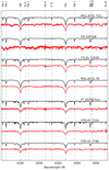 |
Fig. A.2. Disentangled VLT/FLAMES spectra for the newly classified SB2 systems in NGC 6231 (Section 3.1). |
All Tables
Photometry collected of the targets for SED fitting from Sung et al. (2013), Gaia eDR3 (Gaia Collaboration 2016, 2021), and 2MASS (Skrutskie et al. 2006).
All Figures
|
Fig. 1. Phase-folded RV curves and orbital solutions constrained by Banyard et al. (2022) for the SB1s. The five marked with (*) do not pass the Lucy-Sweeney test (e/σe ≤ 2.49) and so are consistent with being circular (we show the eccentric solution). The ephemerises used to phase the RV curves are calculated with the orbital solutions in Table 2, with phase 0 corresponding to the periastron passage. |
| In the text | |
|
Fig. 2. Results from simulated spectra of a mock B2V + A7V binary mimicking the real orbit and data of CPD −41 7717. In green and in red, the synthetic spectra (templates) computed from the stellar parameters of the primary and the secondary components, respectively. The spectra of the secondary have been shifted vertically for clarity. |
| In the text | |
|
Fig. 3. Comparison of the spectroscopic and evolutionary estimates of the compact object candidate SB1s, along with their orbital periods. The dashed line indicates agreement between the two estimates. |
| In the text | |
|
Fig. 4. Computed mass of the unseen companion of the SB1s as a function of the inclination of the system using Eqs. (2) and (4), and using the spectroscopic estimate of the primary mass. The minimum inclination of each system is indicated by the horizontal line, with the associated error as dashed horizontal lines. The vertical line indicates the minimum mass of the unseen companions, with the associated error as dashed vertical lines. The orange shaded regions correspond to the possible values for the system inclinations and the masses of the unseen objects. The red dashed line corresponds to the uncertainty on the binary mass function, computed by propagating the 1σ errors on the other parameters. (a) HD 152200, (b) V* V946 Sco, (c) CD–41 11038, (d) CXOU J165241.3-415536, (e) CPD–41 7717. |
| In the text | |
|
Fig. 5. Same as Fig. 4, but using the evolutionary estimate of the primary mass. (a) HD 152200, (b) V* V946 Sco, (c) CD–41 11038, (d) CXOU J165241.3-415536, (e) CPD–41 7717. |
| In the text | |
|
Fig. 6. TESS light curves, their periodograms, and the light curves phased with the best found period, of five of the targets in which we detected photometric variability. (a) V* V1208 Sco, (b) CPD–41 7717, (c) HD 152200, (d) CXOU J165421.3-415536, (e) CPD–41 7746. |
| In the text | |
|
Fig. 7. Observed cumulative mass-ratio distribution of the SB2 stars in NGC 6231, with the Paper I SB2s as crosses, and the newly disentangled SB2s as stars. The detection probability, calculated from the bias correction of the observational campaign in Paper I, is displayed as a red curve. |
| In the text | |
|
Fig. 8. Orbital period against eccentricity of the B-type binaries in NGC 6231. The SB1s are shown in red, with the candidates for harbouring compact objects in green, the Fourier disentangled SB2s in blue, and the SB2s identified in Paper I in purple. Open faced symbols indicate systems that have eccentricities that do not pass the Lucy-Sweeney test (e/σe ≤ 2.49) and so are consistent with being circular. |
| In the text | |
|
Fig. 9. Estimated spectroscopic (black) and evolutionary (green) masses of each SB1’s unseen companion. The blue zone corresponds to the predicted mass range for Galactic stellar mass BHs and the red zone represents the same but for Galactic NSs (Belczynski et al. 2010; Fryer et al. 2014). The mass ranges for each target where main sequence stars cannot be discounted according to the spectral disentangling sensitivity (Sect. 3.1) are denoted by thick lines. Target names in boldface are the targets for which no companion could be extracted through spectral disentangling, and the other targets are those for which the nature of the extracted companion was ambiguous (Sect. 3.1). |
| In the text | |
|
Fig. 10. Orbital period against projected rotational velocity, v sin i (in black). Red plusses correspond to the critical rotational velocity, vcrit, calculated with Eq. (3). Blue crosses are the computed synchronous rotation rate, vsync, computed for each star assuming they are in a synchronous orbit. |
| In the text | |
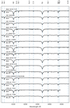 |
Fig. A.1. Shift-and-added VLT/FLAMES spectra for the SB1 targets (Table 2). |
| In the text | |
|
Fig. A.2. Disentangled VLT/FLAMES spectra for the newly classified SB2 systems in NGC 6231 (Section 3.1). |
| In the text | |
Current usage metrics show cumulative count of Article Views (full-text article views including HTML views, PDF and ePub downloads, according to the available data) and Abstracts Views on Vision4Press platform.
Data correspond to usage on the plateform after 2015. The current usage metrics is available 48-96 hours after online publication and is updated daily on week days.
Initial download of the metrics may take a while.