| Issue |
A&A
Volume 667, November 2022
|
|
|---|---|---|
| Article Number | A16 | |
| Number of page(s) | 21 | |
| Section | Interstellar and circumstellar matter | |
| DOI | https://doi.org/10.1051/0004-6361/202243858 | |
| Published online | 03 November 2022 | |
A physically motivated “charge-exchange method” for measuring electron temperatures within H ii regions
1
Astronomisches Rechen-Institut, Zentrum für Astronomie der Universität Heidelberg,
Mönchhofstraße 12-14,
69120
Heidelberg, Germany
e-mail: This email address is being protected from spambots. You need JavaScript enabled to view it.
2
INAF – Osservatorio Astrofisico di Arcetri,
Largo E. Fermi 5,
50157
Firenze, Italy
3
International Centre for Radio Astronomy Research, University of Western Australia,
35 Stirling Highway,
Crawley, WA
6009, Australia
4
Universität Heidelberg, Zentrum für Astronomie, Institut für Theoretische Astrophysik,
Albert-Ueberle-Str 2,
69120
Heidelberg, Germany
5
Universität Heidelberg, Interdisziplinäres Zentrum für Wissenschaftliches Rechnen,
Im Neuenheimer Feld 205,
69120
Heidelberg, Germany
6
Center for Astrophysics and Space Sciences, Department of Physics, University of California,
San Diego, 9500 Gilman Drive,
La Jolla, CA
92093, USA
7
Argelander-Institut für Astronomie, Universität Bonn,
Auf dem Hügel 71,
53121
Bonn, Germany
8
Department of Physics and Astronomy, University of Wyoming,
Laramie, WY
82071, USA
9
Research School of Astronomy and Astrophysics, Australian National University,
Canberra, ACT
2611, Australia
10
Max-Planck-Institut für Astronomie,
Königstuhl 17,
69117
Heidelberg, Germany
Received:
25
April
2022
Accepted:
21
July
2022
Abstract
Aims. Temperature uncertainties plague our understanding of abundance variations within the interstellar medium. Using the PHANGS-MUSE large program, we develop and apply a new technique to model the strong emission lines arising from H ii regions in 19 nearby spiral galaxies at ~50 pc resolution and infer electron temperatures for the nebulae.
Methods. Due to the charge-exchange coupling of the ionization fraction of the atomic oxygen to that of hydrogen, the emissivity of the observed [O i]λ6300/Hα line ratio can be modeled as a function of the gas phase oxygen abundance (O/H), ionization fraction (fion), and electron temperature (Te). We measure O/H using a strong-line metallicity calibration and identify a correlation between fion and [S iii]λ9069/[S ii]λ6716,6730, tracing ionization parameter variations.
Results. We solve for Te and test the method by reproducing direct measurements of Te([N ii]λ5755) based on auroral line detections to within ~600 K. We apply this“charge-exchange method” of calculating Te to 4129 H ii regions across 19 PHANGS-MUSE galaxies. We uncover radial temperature gradients, increased homogeneity on small scales, and azimuthal temperature variations in the disks that correspond to established abundance patterns. This new technique for measuring electron temperatures leverages the growing availability of optical integral field unit spectroscopic maps across galaxy samples, increasing the statistics available compared to direct auroral line detections.
Key words: HII regions / ISM: abundances / galaxies: ISM / ISM: atoms / ISM: clouds / ISM: general
© K. Kreckel et al. 2022
 Open Access article, published by EDP Sciences, under the terms of the Creative Commons Attribution License (https://creativecommons.org/licenses/by/4.0), which permits unrestricted use, distribution, and reproduction in any medium, provided the original work is properly cited.
This article is published in open access under the Subscribe-to-Open model. This email address is being protected from spambots. You need JavaScript enabled to view it. to support open access publication.
1 Introduction
Star formation is regulated by the complex interplay of heating and cooling processes in the interstellar medium (ISM). The gaseous clouds that provide the raw materials for stars to form must cool sufficiently so that they can condense and collapse (McKee & Ostriker 2007; Klessen & Glover 2016). However, the resulting stars proceed to ionize and heat their surroundings, with the most massive stars contributing further mechanical energy and enriched materials at the end of their life via supernovae, feeding it back into their natal environment (Maiolino & Mannucci 2019). This cycling of baryons on small scales is reflected by the temperature transitions from the dense cold molecular gas (~ 10 K) and the warm ionized medium (~ 10 000 K) found in H ii regions to the super-heated shock waves driven by supernova explosions (~106 K).
In particular, within H ii regions the electron temperature reflects not just the strength and hardness of the ionizing radiation field (O stars have temperatures up to ~50 000 K), but the ability of the gas to efficiently cool through collisionally excited lines arising from heavierelements (e.g., carbon, oxygen, and nitrogen). In fact, the balance between heating and cooling in these nebulae predominantly reflects the metal abundance present in the surrounding ISM (Osterbrock & Ferland 2006), although age variations also play some role (Ho et al. 2019).
Direct measurement of electron temperatures is possible using faint temperature-sensitive emission lines. In the radio, it is possible to use radio recombination lines to derive the electron temperatures for H ii regions. However, these lines are very weak, and while such observations are possible for Milky Way targets (Balser et al. 2015; Wenger et al. 2019; Pineda et al. 2019), they remain challenging for extragalactic targets (Zhao et al. 1996; Kepley et al. 2011; Luisi et al. 2018; Kewley et al. 2019). In the optical one can observe auroral lines (e.g., [O iii]λ4363, [N ii]λ5755, [S iii]λ6312, and [O ii]λ7320,7330) in extragalactic systems, but they are also very faint, typically around ~1% of their strong line counterparts. Extensive long-slit observational projects have attempted to detect auroral lines across large samples of H ii regions in nearby galaxies, but collecting statistically significant samples of these faint lines is challenging. Observational campaigns targeting low-mass, metal-poor galaxies such as M33, where the auroral lines are brighter, can accumulate relatively large numbers of detections (e.g., 61 H ii regions with [O iii]λ4363 detections; Rosolowsky & Simon 2008), but this approach remains daunting for high-mass systems. In the CHemical Abundances of Spirals (CHAOS) project, initial results from Berg et al. (2020) detect auroral lines for a total of 190 H ii regions across four galaxies, where they are able to make direct measurements of the electron temperatures.
With the advent of wide-field optical integral field spec-trographs on large 8-meter class telescopes, it is now feasible to systematically observe much larger samples of H ii regions with auroral line detections, but the telescope time requirements remain high. Four hours spent surveying NGC 1672 with the Multi Unit Spectroscopic Explorer (MUSE) on the Very Large Telescope (VLT) resulted in ~80 H ii regions with [N ii]λ5755 auroral line detections (Ho et al. 2019). As such, direct detections of tens of auroral lines per galaxy have become feasible but remain expensive.
In addition to these auroral line measurements remaining extremely challenging, with only tens of H ii regions we cannot uniformly sample the galaxy disks. Increased statistics on temperature (and metallicity) variations provide insights into the evolutionary processes regulating gas flows and galaxy evolution (Kreckel et al. 2019, 2020; Sánchez-Menguiano et al. 2019; Ho et al. 2019; Li et al. 2021) but remain plagued by the systemat-ics affecting strong-line metallicities. We explore a new method to constrain the electron temperature, based on a combination of strong lines, with the goal of increasing the number of regions within which measurements of the electron temperature are possible. We present an overview of the physical motivation for the method in Sect. 2. We describe the data used in Sect. 3 and develop and validate our new method in Sect. 4. We discuss the results in Sect. 5 and conclude in Sect. 6.
2 Physical motivation for the method
Nature has gifted us with a convenient coincidence. The ion-ization potential of oxygen (13.618 eV) is very similar to the ionization potential of hydrogen (13.598 eV). As such, the charge-exchange reaction O0 +H+ ↔ O++H0 is very efficient, and acts to couple the ionization fraction of oxygen to the ionization fraction of hydrogen (see, e.g., Draine 2011; Tielens 2010). This means that the number densities (which we denote as n(X), for species X) of oxygen and hydrogen are related by
 (1)
(1)
where
 (2)
(2)
and
 (3)
(3)
It should be noted that we define the ionization fraction of hydrogen as
 (4)
(4)
Therefore, for line emission associated with the relevant ions,
![Mathematical equation: ${{\left[ {{\rm{O I}}} \right]\lambda 6300} \over {{\rm{H}}\alpha }} \propto {{n\left( {{{\rm{O}}^0}} \right)} \over {n\left( {{{\rm{H}}^ + }} \right)}} = {{n\left( {\rm{O}} \right)} \over {n\left( {\rm{H}} \right)}}{{n\left( {{{\rm{H}}^0}} \right)} \over {n\left( {{{\rm{H}}^ + }} \right)}} = {{n\left( {\rm{O}} \right)} \over {n\left( {\rm{H}} \right)}}{{1 - {f_{{\rm{ion}}}}} \over {{f_{{\rm{ion}}}}}}.$](/articles/aa/full_html/2022/11/aa43858-22/aa43858-22-eq5.png) (5)
(5)
This is significant as the line ratio [O i]/Hα depends only on temperature (through the proportionality pre-factor), metallicity (n(O)/n(H)) and the ionization fraction of hydrogen (fion).
Using the latest calculations of the [O i] and Hα emission rates (Barklem 2007; Dong & Draine 2011), we derive the emis-sivity of [O i]λ6300 relative to Hα (as outlined in Appendix A) to be
![Mathematical equation: $\matrix{ {{{\left[ {{\rm{OI}}} \right]\lambda 6300} \over {{\rm{H}}\alpha }}} \hfill & { = 8492{{{f_{{\rm{OI}}}}\left( T \right)} \over {T_4^{ - 0.942 - 0.031\ln {T_4}}}}\exp \left( { - {{2.284} \over {{T_4}}}} \right)} \hfill \cr {} \hfill & { \times {{n\left( {\rm{O}} \right)} \over {n\left( {\rm{H}} \right)}}} \hfill \cr {} \hfill & { \times {{n\left( {{{\rm{H}}^0}} \right)} \over {n\left( {{{\rm{H}}^{\rm{ + }}}} \right)}}\xi ,} \hfill \cr } $](/articles/aa/full_html/2022/11/aa43858-22/aa43858-22-eq6.png) (6)
(6)
where T4 is the electron temperature (Te) in units of 10 000 K, foi is defined as
 (7)
(7)
where the coefficients ai are listed in Table 1, and ξ is a function of the hydrogen ionization ratio
 (8)
(8)
This factor ξ is just above unity and ranges from 1 to 9/8. This equation holds if the [O i] and Hα emission are co-spatial, arising from the same parcel of gas. We discuss this in more detail below, and explore the implications of this assumption in Sect. 5.3.1. This is an update to the relation provided in Reynolds et al. (1998).
The aim of this paper is to utilize a measurement of [O i]/Hα, combined with an estimate of fion, to infer Te. While Te can be directly measured through the detection of faint auroral lines, there exist no well-established prescriptions to infer fion from observations of strong lines. In this paper, we determine an empirical relation between fion and strong line diagnostic ratios in order to allow us to solve for Te. This “charge-exchange method” of determining Te represents a novel approach that may be widely applicable to existing data sets. We develop our method using a set of line fluxes measured arising from integrated H ii regions, as extragalactic H ii regions are generally unresolved.
For this charge-exchange method to apply, we assume that electron collisions dominate the excitation of the [O i] line, rather than collisions with atomic hydrogen. The critical fractional ionization above which electron collisions dominate is ~10−3−10−4, which we expect to be true for the H ii regions we consider. We also assume that the emitting regions are in the low density limit, rather than the local thermodynamic equilibrium limit. Since the critical density is ~106 cm−3, this should also be valid for all of the H ii regions we consider.
There are limitations to this method that are worth highlighting here, and that will be addressed in more detail in Sect. 5.2. This model compares the [O i] and Hα line emission. However, while the majority of the hydrogen in an H ii region is ionized and emitting in Hα, [O i] will be emitted mainly in an outer shell near the ionization front. In applying this method, we are assuming that Te is uniform across both the Hα and [O i] emitting regions. Ideally, we would further consider emission that is co-spatial, arising from the same parcel of gas. However, for unresolved H ii regions, we can consider only emission integrated across the entire nebula. In our approach, we argue that fion constrains the size of the partially ionized zone, accounting for this discrepancy in emitting zones. Over larger (kiloparsec-scale) regions of the diffuse ionized gas, the radiation field is more diluted (low ionization parameter) and therefore the partially ionized zone is wider and would lead to a better correspondence between Hα and [O i] emitting regions.
This technique was initially developed in relation to diffuse ionized gas in the Milky Way (Reynolds et al. 1998), and later applied to four individual H ii regions in the Milky Way (Hausen et al. 2002). We further develop this method, and aim to apply it to the thousands of H ii regions within the PHANGS-MUSE sample. [O i] emission can be challenging to measure, as it is faint and can be blended with the strong and highly variable telluric airglow emission. In this work we target nearby (~10–20 Mpc) galaxies with sufficiently large velocity offset from terrestrial [O i], and with sufficient depth to detect [O i] across a wide sample of H ii regions. Here, we explore the regime where an entire H ii region is integrated over 50–100 pc scales. While the main goal is to infer Te, we note that we need to assume a metallicity in order to apply the charge-exchange method. Therefore, our Te measurement is dependent on the assumed strong-line metallicity, and using it to infer metallicities using the direct method would be circular. We test the metallicity dependence of the method in Sect. 4.4. Some iterative approach may be suitable, but this is beyond the scope of this work.
3 Data
3.1 CHAOS
To develop our method, we explored data from the CHAOS project. Berg et al. (2020) summarizes the latest results (see also Berg et al. 2015; Croxall et al. 2015, 2016), including four galaxies (NGC 628, NGC 3184, M 51, and M 101) with a total of 190 H ii regions with auroral line detections as measured from integrated H ii region spectra. Of these, 121 have detections of [N ii]λ5755, 131 have [S iii]λ6312, 154 have [O ii]λ7320,7330, and 72 have [O iii]λ4363. These auroral lines, arising from high energy levels, are used in combination with the nebular lines from lower energy levels of the same ion to compute electron temperatures for each ion. Using different ions to represent different temperatures across ionization zones in the nebulae, Berg et al. (2020) combined these measurements to compute the oxygen abundance, 12+log(O/H), using the direct method. In this way, from the CHAOS data set, we have measurements of Te and O/H for 190 H ii regions, as well as a full catalog of strong emission lines ([O ii]λ3727,3729, [O iii]λ5007, Hβ, [O i]λ6300, [N ii]λ6583, Hα, [S ii]λ6716,6730, and [S iii]λ9069). All line fluxes from their catalog have been corrected for extinction using the Balmer series (Hα, Hβ).
These observations were carried out using the Multi-Object Double Spectrographs (MODS; Pogge et al. 2010) with slit masks on the Large Binocular Telescope (LBT). Slits placed on individual H ii regions were designed to be 1” wide and 10” long. This slit width is well matched to the seeing during observations; however, as the brightest H ii regions are typically selected, this does not necessarily encompass the full H ii region size, which for giant H ii regions can be as large as ~100 pc (Azimlu et al. 2011; Mannucci et al. 2021). At the 7–11 Mpc distances of the four targets this slit width corresponds to 1″ = 30–50 pc, such that some slit losses may be expected. No correction is applied to account for the local diffuse ionized gas (DIG) background emission.
3.2 PHANGS-MUSE
After initial investigations into the charge-exchange method using the CHAOS data, we develop and test our method using H ii regions selected from the PHANGS-MUSE data set (Emsellem et al. 2022; Groves et al., in prep.). The Physics at High Angular resolution in Nearby GalaxieS (PHANGS) collaboration has targeted nearby spiral disk galaxies along the star-forming main sequence (Table 2). Targets were selected to be nearby (D < 19 Mpc, 1″ < 100 pc) and moderately inclined (inclination <60°). Observations of 19 galaxies were carried out using the VLT/MUSE (Bacon et al. 2010) instrument primarily as part of a MUSE large program (PI: Schinnerer), which observed 172 individual MUSE pointings across these 19 galaxies over 4800–9300 Å at <1″ resolution. The data reduction pipeline and data analysis pipeline used to reduce this data set and extract emission line maps are described in detail in Emsellem et al. (2022). This results in an optical integral field spectroscopic data cube, as well as integrated line emission maps of a wide range of both strong ([O iii]λ5007, Hβ, [O i]λ6300, [N ii]λ6583, Hα, [S ii]λ6716,6730, and [S iii]λ9069) and auroral ([N ii]λ5755, [S iii]λ6312, and [O ii]λ7320,7330) emission line fluxes. For the [O iii] and [N ii] doublets we measure only the stronger line, and for the [S iii] doublet we measure only the bluer line, and assume fixed atomic ratios (Osterbrock & Ferland 2006; Tayal et al. 2019) as
![Mathematical equation: $\matrix{ {\left[ {{\rm{O}}\,{\rm{III}}} \right]\lambda 6548} & = & {0.35 \times \left[ {{\rm{N}}\,{\rm{III}}} \right]\lambda 6584} \cr {\left[ {{\rm{N}}\,{\rm{II}}} \right]\lambda 65448} & = & {0.34 \times \left[ {{\rm{N}}\,{\rm{II}}} \right]\lambda 6584} \cr {\left[ {{\rm{S}}\,{\rm{III}}} \right]\lambda 9532} & = & {2.5 \times \left[ {{\rm{S}}\,{\rm{III}}} \right]\lambda 9069.} \cr } $](/articles/aa/full_html/2022/11/aa43858-22/aa43858-22-eq9.png) (9)
(9)
Using the Hα emission line maps, Santoro et al. (2022) morphologically identified individual nebular regions using the HIIPHOT package (Thilker et al. 2000), using a technique similar to that described in Kreckel et al. (2019). This works by identifying peaks in the Hα distribution, and growing those peaks until a neighboring region is encountered or a termination criterion set by the flux gradient is reached. These nebular region masks are then applied to the original data cube, and the spectra within each nebular region are summed and refit using the data analysis pipeline. The resulting nebular catalog compiles a list of objects with their associated line fluxes, extinction corrected using the Balmer decrement, with approximately 31 000 regions identified across the full sample. All galaxies are at sufficiently high systemic velocities (υsys > 650 km s−1) that the critical [O i] emission line is not blended with telluric airglow (Table 2).
We applied the standard BPT (Baldwin et al. 1981) diagnostic diagrams, requiring S/N > 3 for all relevant lines, and constructed our H ii region catalog by selecting those regions from the nebular catalog that are consistent with both of the pho-toionization demarcations given by Kauffmann et al. (2003) in the [O iii]/Hβ versus [N Il]/Hα diagram and the Kewley et al. (2001) lines in the [O iii]/Hβ versus [S Il]/Hα diagram. Regions that have S /N < 3 in any of the relevant diagnostic lines are excluded from the sample. We further exclude H ii regions within one 1″ of the field edge or a foreground star. This results in an H ii region catalog consisting of ~24 000 objects. Given that the median size of our H ii regions is approximately consistent with our seeing limit, we expect that most of these H ii regions are unresolved. In this sense, we always contain the full spatial extent of the H ii region in our integrated spectrum.
The PHANGS-MUSE spectra also include detections of the faint [N ii] λ5755 auroral line (Ho et al. 2019). Fitting of this faint line (typically less than 1% of the Hα line flux) is carried out using the integrated H ii region spectra, subtracting the stellar population fit, and performing a Gaussian fit on the residual. Given the faintness of the line, very slight offsets in the stellar population fitting can result in systematic residuals at the location of the [N ii] line. To improve the flux estimate from our Gaussian fit, we fix the velocity centroid to have the same systemic velocity as we measure for the brighter Hα line, but additionally allow for a local linear background to account for systematics in the stellar population fit. Errors are determined by sampling the error spectrum and repeating this analysis 100 times. This results in ~840 H ii regions where the [N ii] λ5755 line is detected at S /N >10. As with the other measured lines, we correct for extinction in using the Balmer decrement, combine this with the de-reddened measurement of [N ii] λ6583 and use PYNEB (Luridiana et al. 2015) assuming ne = 10 cm−3, consistent with the measured values (Barnes et al. 2021), to compute Te([N ii]).
For the fainter and unresolved regions the DIG background may introduce uncertainties in recovering the intrinsic line fluxes. In order to measure the DIG contribution at the position of each H ii region, we mask out all nebular regions and compute the median line flux within a 10″ ×10″ box around each region for the lines most strongly emitted by the DIG (Hβ, [O i], Ha, [N ii], [S ii]). We require a 3σ detection of a DIG signal in order to include it in our calculations. As implementing the DIG subtraction is a fairly uncertain process, we do not attempt any DIG subtraction. Instead, we aim to minimize the impact of the DIG on our measurements by requiring that H ii regions have a >50% contrast of all lines against the surrounding DIG background. Approximately 35% of all H ii regions do not have significant detections in all necessary emission lines against the DIG background, and are excluded from further analysis.
Properties of the galaxies in the PHANGS-MUSE sample.
3.3 Strong line O/H abundances
As this method relies on knowing O/H, we apply a strong line abundance prescription to both the CHAOS and PHANGS H ii region catalogs. Our preferred strong line abundance prescription is the S calibration from Pilyugin & Grebel (2016), an empirical method that relies on the combination of three diagnostic line ratios. This provides an improved ability to remove degeneracies between metallicity and ionization parameter when compared to prescriptions that use only one or two diagnostic ratios (for some discussion see Ho 2019; Kreckel et al. 2019). It has been shown to produce qualitatively similar results to the Dopita et al. (2016) N2S2 prescription (Kreckel et al. 2019), and achieves small systematic uncertainties (Metha et al. 2021).
The S calibration relies on the following three standard diagnostic line ratios:
![Mathematical equation: $\matrix{{{{\rm{N}}_2}} & = & {{{\left( {\left[ {{\rm{N}}\,{\rm{II}}} \right]\lambda 6548 + \lambda 6584} \right)} \mathord{\left/ {\vphantom {{\left( {\left[ {{\rm{N}}\,{\rm{II}}} \right]\lambda 6548 + \lambda 6584} \right)} {{\rm{H}}\beta ,}}} \right. \kern-\nulldelimiterspace} {{\rm{H}}\beta ,}}} \cr {{{\rm{S}}_2}} & = & {{{\left( {\left[ {{\rm{S}}\,{\rm{II}}} \right]\lambda 6717 + \lambda 6731} \right)} \mathord{\left/ {\vphantom {{\left( {\left[ {{\rm{S}}\,{\rm{II}}} \right]\lambda 6717 + \lambda 6731} \right)} {{\rm{H}}\beta ,}}} \right. \kern-\nulldelimiterspace} {{\rm{H}}\beta ,}}} \cr {{R_3}} & = & {{{\left( {\left[ {{\rm{O}}\,{\rm{III}}} \right]\lambda 4959 + \lambda 5007} \right)} \mathord{\left/ {\vphantom {{\left( {\left[ {{\rm{O}}\,{\rm{III}}} \right]\lambda 4959 + \lambda 5007} \right)} {{\rm{H}}\beta }}} \right. \kern-\nulldelimiterspace} {{\rm{H}}\beta }}.} \cr }$](/articles/aa/full_html/2022/11/aa43858-22/aa43858-22-eq10.png) (10)
(10)
The prescription is defined separately over the upper and lower branches in log N2. The upper branch (log N2 ≥ −0.6) is calculated as
 (11)
(11)
and the lower branch (log N2 < −0.6) is calculated as
 (12)
(12)
4 Method development
Using the four galaxies in the CHAOS data set, we begin by using their measured [O i]/Hα, Te based on auroral line detections, and direct method metallicity in order to infer fion for each of their H ii regions (Fig. 1). This direct method metallicity is derived by associating different Te values to different ionization zones in the nebula, such that the final metallicity is not independent of the Te measurements. Using the S calibration to derive metallicities provides similar results, although with increased scatter. Based on the auroral line detections of [N ii], [O ii], [O iii], and [S iii], this approach provides four different measurements of Te, reflecting the ionic temperature in the zone where each ion is dominant. We find fion values ranging from 0.93 to 0.99, and a median value of fion = 0.97 across all H ii regions.
As we are integrating over the entire H ii region, although [O i] is not emitted throughout the entire nebula, we expect that fion will change systematically with the ionization structure of the nebulae and the size of the partially ionized region. To that end, we looked for correlations with line ratios that depend on changes in the ionization parameter,
 (13)
(13)
where Q(H0) is the number of ionizing photons emitted per second, R is the distance between the central source and the emitting material and n(H) is the hydrogen density. In photoionization models, the ionization parameter q correlates linearly with the log of [O iii]/[O ii], [S iii]/[S ii], and [O ii]/Hβ, with both [O iii]/[O ii] and [O iii]/Hβ showing additional dependences on metallicity (Kewley & Dopita 2002; Dors et al. 2011). We note that here we define:
![Mathematical equation: $\matrix{ {{{\left[ {{\rm{O}}\,{\rm{III}}} \right]} \mathord{\left/ {\vphantom {{\left[ {{\rm{O}}\,{\rm{III}}} \right]} {\left[ {{\rm{O}}\,{\rm{II}}} \right]}}} \right. \kern-\nulldelimiterspace} {\left[ {{\rm{O}}\,{\rm{II}}} \right]}}} & = & {{{\left[ {{\rm{O}}\,{\rm{III}}} \right]\lambda 5007} \mathord{\left/ {\vphantom {{\left[ {{\rm{O}}\,{\rm{III}}} \right]\lambda 5007} {\left[ {{\rm{O}}\,{\rm{II}}} \right]}}} \right. \kern-\nulldelimiterspace} {\left[ {{\rm{O}}\,{\rm{II}}} \right]}}\lambda 3726,3729} \cr {{{\left[ {S\,{\rm{III}}} \right]} \mathord{\left/ {\vphantom {{\left[ {S\,{\rm{III}}} \right]} {\left[ {{\rm{S}}\,{\rm{II}}} \right]}}} \right. \kern-\nulldelimiterspace} {\left[ {{\rm{S}}\,{\rm{II}}} \right]}}} & = & {{{\left[ {{\rm{S}}\,{\rm{III}}} \right]\lambda 9069,9532} \mathord{\left/ {\vphantom {{\left[ {{\rm{S}}\,{\rm{III}}} \right]\lambda 9069,9532} {\left[ {{\rm{S}}\,{\rm{II}}} \right]\lambda 6717,6731}}} \right. \kern-\nulldelimiterspace} {\left[ {{\rm{S}}\,{\rm{II}}} \right]\lambda 6717,6731}}} \cr {{{\left[ {{\rm{O}}\,{\rm{III}}} \right]} \mathord{\left/ {\vphantom {{\left[ {{\rm{O}}\,{\rm{III}}} \right]} {{\rm{H}}\beta }}} \right. \kern-\nulldelimiterspace} {{\rm{H}}\beta }}} & = & {{{\left[ {{\rm{O}}\,{\rm{III}}} \right]\lambda 5007} \mathord{\left/ {\vphantom {{\left[ {{\rm{O}}\,{\rm{III}}} \right]\lambda 5007} {{\rm{H}}\beta .}}} \right. \kern-\nulldelimiterspace} {{\rm{H}}\beta .}}} \cr }$](/articles/aa/full_html/2022/11/aa43858-22/aa43858-22-eq14.png) (14)
(14)
We find a strong correlation between fion and [S iii]/[S ii] (as a proxy for ionization parameter) for all four ions (Fig. 1), with Te([N ii]) producing the strongest correlation (as judged by the Spearman’s rank correlation coefficient, ρ = 0.67). This is reasonable, as the temperature of the ion tracing the low-ionization zone of the nebula is best suited to describe the [O i] emitting region (Berg et al. 2020; see also Sect. 5.2). It also shows the most uniform trend across all four galaxies in the sample. Given the strong correlation and relatively high number of detections, we chose to adopt Te([N ii]) as a reference temperature for the rest of the analysis in this paper.
Weaker correlations are seen with [O iii]/Hβ or [O iii]/[O ii](ρ ~ 0.5, Fig. 2). Some correlations are also seen with the input parameters used in calculating f on (Fig. 3), showing the strongest correlation with [O i]/Hα (ρ = −0.57) and a weaker correlation with Te([N ii]) (ρ = 0.24). No significant correlation is seen with 12+log(O/H), suggesting fion is relatively insensitive to changes in abundance.
4.1 Aperture biases
While the CHAOS data set presents a remarkable catalog of emission lines and derived properties, by design it is targeting only the central regions of the brightest H ii regions in order to improve the chances of detecting the faint auroral lines. We note that in Fig. 1, the majority of CHAOS H ii regions have [S iii]/[S ii] > 1.0. These are relatively high compared to what is reported in samples that probe fainter H ii regions (e.g., Kreckel et al. 2019; Mingozzi et al. 2020). In particular, the incomplete spatial coverage of any given H ii region results in an inherent bias for line ratio diagnostics that show radial structure within a H ii region. This is apparent in the [S iii]/[S ii] line ratio, as CHAOS observations probe only the central ~50 pc (~1″) of the nebulae, where the [S iii] emission is strongest, and miss [S ii] emission in the outer nebulae (see also Mannucci et al. 2021).
We demonstrate this directly by cross matching the H ii regions cataloged by CHAOS and by PHANGS-MUSE in NGC 628, the only galaxy contained in both samples. As CHAOS is predominantly targeting the outer disk while PHANGS-MUSE is limited to the inner disk, only 13 H ii regions overlap between the two samples. In Fig. 4 we compare the [S iii]/[S ii] line ratios, and demonstrate how the aperture bias results in systematically higher measurements in the CHAOS sample. This offset persists even when accounting for differences in the assumed reddening E(B−V) (due to both the foreground Milky Way and local reddening within the galaxy) adopted in the two surveys. Challenges such as this motivate our use of integrated H ii region spectra for this paper, but similarly prevent us from relying solely on the CHAOS sample for the determination of an empirical relation between fion and [S iii]/[S ii].
Of the 13 H ii regions, only 11 have detections of [N ii]λ5755, and subsequent calculations of Te([N ii]), in both samples. In Fig. 5 we show a comparison of the derived Te([N ii]), which follows very well the one-to-one line within the uncertainties. This agreement speaks to a smooth and roughly constant temperature structure within the [N ii] emitting region, as expected, as well as the high fidelity in both data sets.
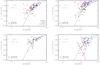 |
Fig. 1 For the CHAOS H ii regions: fion modeled based on Eq. (6), assuming different input electron temperatures based on auroral line measurements (Te([N ii]), Te([O ii]), Te([O iii]), and Te([S iii])) as well as their reported 12+log(O/H) and [Ο i]/Ηα. Each of the four galaxies is shown with separate symbols, and the Spearman's rank correlation coefficient (ρ) and its significance (p) are shown in each figure. Each value of fion is plotted as a function of the [S iii]/[S ii] line ratio, which robustly traces changes in the ionization parameter (Kewley & Dopita 2002). We identify Te([N ii]) as showing the strongest correlation (ρ = 0.69) and a large number of detections and therefore chose to adopt Te([N ii]) as a reference temperature for the rest of the analysis in this paper. The dashed line shows the fit derived in Sect. 4.2, using a combination of PHANGS-MUSE and CHAOS Η ii regions. This same line is overplotted for the other panels (dashed lines) to allow comparison across the ionic temperatures. |
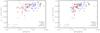 |
Fig. 2 Demonstration of further (weaker) correlations between fion and line ratios, tracing changes in the ionization parameter ([Ο iii]/Ηβ, left; [O iii]/[O ii], right) for Η ii regions in the CHAOS sample while using Te([N ii]) as our fiducial temperature measurement. Each of the four galaxies is shown with separate symbols, and the Spearman's rank correlation coefficient (ρ) and its significance (p) are shown in each figure. Weaker correlations (ρ ~ 0.5) compared to the correlations with [S iii]/[S ii] (Fig. 1) are seen. |
4.2 Parameterizing fion
From the CHAOS sample, it is clear that changing the size of the partially ionized zone within the H ii region corresponds to a change in ionization parameter, with the strongest correlation identified between fion when measured using Te([N ii]), and [S iii]/[S ii] (as a proxy for ionization parameter). As expected from models, the ionization fraction (i.e., basically the extent of the partially ionized zone) correlates with ionization parameter. However, given the aperture bias, we cannot employ the measurements of [S iii]/[S ii] from CHAOS when determining an empirical relation. We therefore used the 840 H ii regions from PHANGS-MUSE that have Te([Ν ii]) measurements to determine an empirical relation, such that we can use the observed [S iii] and [S ii] emission to constrain fion. With this prescription we will then be able to measure all three necessary parameters (fion, 12+log(O/H) and [Ο i]/Ha) using strong line methods and thus solve for Te.
In Fig. 6 we show fioa as a function of [S iii]/[S ii] for the full PHANGS-MUSE Η ii region sample (points). We impose the requirement that regions be detected against the DIG background by at least a 50% contrast, and consider only regions with [S iii]/[S ii] > 0.5, where our sample appears more complete (filled circles). We also show the Η ii regions from all four galaxies from the CHAOS sample (open circles), which, due to aperture biases, have systematically overestimated [S iii]/[S ii] line ratios compared to the MUSE data (see Fig. 4), but nonetheless form a nearly continuous sequence with the PHANGS-MUSE H ii regions. Given the nonlinear shape in this relation, it is apparent that a linear extrapolation from the CHAOS measurements (preferentially biased to high [S iii]/[S ii]) would not be suitable for the bulk of the PHANGS-MUSE sample (seen also in Fig. 1). However, given the smooth transition across samples, this also suggests that the correlation holds even when considering changes in fion and changes in ionization parameter within the nebulae. To determine the most widely applicable fit, we combined the PHANGS-MUSE and CHAOS samples and constructed bins in [S iii]/[S ii] requiring a minimum of 10 data points, to demonstrate the median trend across the sample (red line, Fig. 6). To this median trend, we fitted a third order power law where we have fixed the asymptote to fion = 1.0. This shows very good agreement with the binned median, and is parameterized by
![Mathematical equation: ${f_{{\rm{ion}}}} = 1.0 + {c_1} \times {\left( {{{\log }_{10}}\left( {{{\left[ {{\rm{SIII}}} \right]} \mathord{\left/ {\vphantom {{\left[ {{\rm{SIII}}} \right]} {\left[ {S{\rm{II}}} \right]}}} \right. \kern-\nulldelimiterspace} {\left[ {S{\rm{II}}} \right]}}} \right) - {c_2}} \right)^3},$](/articles/aa/full_html/2022/11/aa43858-22/aa43858-22-eq15.png) (15)
(15)
where c1 = 0.0139 ± 0.0060 and c2 = 1.4119 ± 0.1890.
We further overplot this fit on the relations in Fig. 1 for the CHAOS data, and see reasonable agreement with many of the different ionic temperatures. The trend is reasonably consistent with Te([N ii]), Te([S iii]), and Te([O iii]), but clearly offset from Te([O ii]). This reflects some of the previously reported discrepancies between different ionization zones (Berg et al. 2020), though it is somewhat surprising that [O iii] (a very high ionization tracer) would work better than, for example, [O ii] (a low-ionization tracer).
Given that we have imposed a minimum value of [S iii]/[S ii] > 0.5, we cannot extrapolate this relation to lower [S iii]/[S ii] without additional data or modeling. We revisit this decision in Sect. 5.3.
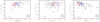 |
Fig. 3 Correlating fion with the three input parameters (Te([Ν ii]), 12+log(O/H), and [Ο i]/Ηα) for each H ii region in the CHAOS sample. Each of the four galaxies is shown with separate symbols, and the Spearman’s rank correlation coefficient (ρ) and its significance (p) are shown in each figure. The fion variations correlate most strongly with changes in [Ο i]/Ηα, but show a weaker correlation than the trends with [S iii]/[S ii] in Fig. 1. |
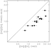 |
Fig. 4 Comparison of the [S iii]/[S ii] line ratio measured across integrated Η ii region spectra from PHANGS-MUSE with the measurement obtained within the CHAOS 1″ slit for 13 H ii regions that overlap between the two surveys. Error bars are shown for both surveys, although the PHANGS errors are smaller than the symbols. The one-to-one line (black) shows that CHAOS systematically overestimates the line ratio by focusing on only the central brightest part of these extended Η ii regions, where the [S iii] emission is preferentially located. This demonstrates the challenges of applying such resolved measurements to broader Η ii region samples. |
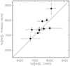 |
Fig. 5 Comparison of Te([N ii]) measured in integrated H ii region spectra from PHANGS-MUSE with equivalent measurements from the CHAOS 1″ slit for ten H ii regions that have reported [N ii]5755 line detection in both surveys. We observe good systematic agreement between the two measurements. |
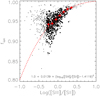 |
Fig. 6 As in Fig. 1, fion modeled assuming the values of Te([N ii]) measured from direct detection of auroral lines in the PHANGS-MUSE Η ii region sample (points). This forms a continuous sequence with the Η ii regions in the CHAOS sample (open circles), but with a significantly more pronounced nonlinear trend. From the PHANGS-MUSE sample, we selected only regions with a more than 50% contrast against the DIG background and with [S iii]/[S ii] > 0.5 (filled circles). We then combined the PHANGS-MUSE and CHAOS samples to construct a binned median (red circles). We fit this with the functional form described in Eq. (15) (dashed red line) to determine our empirical relation for fion. |
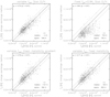 |
Fig. 7 Comparison of the modeled Te as a function of the Te measured within PHANGS-MUSE using the [N ii] λ5755 auroral line. Each panel makes different assumptions about how the values of fion or 12+log(O/H) are calculated. For each panel we show a one-to-one relation (solid line) and 1σ relative scatter (dotted lines), as well as the Spearman’s rank correlation coefficient (ρ). Top left: demonstration of our adopted method (Sect. 4.3), where we use our empirical prescription for fion (Eq. (15)) and metallicities calculated from the strong line Scal method. We recover high correlations (ρ = 0.79) and systematic agreement within 6 K, with a scatter of 546 K. Relaxing various assumptions in our model increases the scatter. Top right: assuming a fixed fion = 0.94 (the median for the PHANGS-MUSE sample), which produces significantly higher scatter (~755 K) and clear deviations from the one-to-one relation. Bottom panels: with variable fion applied but our derivation of 12+log(O/H) relaxed, with either a linear radial gradient (left) or a fixed metallicity adopted for each galaxy (right). Both recover high correlation coefficients with moderately increased scatter (~600 K). This demonstrates the relative insensitivity to the input metallicity for this charge-exchange method of deriving Te. |
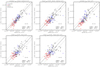 |
Fig. 8 Comparison of the modeled Te as a function of Te measured by CHAOS using the [N ii] λ5755 auroral line. Each panel makes a different assumption about how the value of fion and 12+log(O/H) are calculated. The top-left plot represents the best-case scenario, where we vary fion as a function of [S iii]/[S ii] and use metallicities calculated from the direct method. This shows the lowest systematic scatter between Te values of 662 K. The other two plots in the top row each relax one of the assumptions, assuming either a fixed fion = 0.97 (top center) or a metallicity calculated from strong line techniques (top right). Both have an increased scatter of ~900 K. The two plots in the bottom row further relax the assumptions, resulting in further inaccuracies. This test includes the assumptions of both a fixed fion = 0.97 and a strong-line metallicity (~950 K; bottom right) and a fixed fion = 0.97 and a fixed global metallicity per galaxy (~1100 K; bottom center). A one-to-one relation (solid line) and 1σ scatter (dotted lines) are shown in each plot, and the median and standard deviation are listed. While relaxing our assumptions does result in increased scatter, the overall agreement remains good. We adopt the assumptions that go into the top-right figure (a variable fon and a strong line 12+log(O/H)) for the model that we apply in this work, as summarized in Sect. 4.3. |
4.3 Method summary
We summarize here the conditions that must be met in order to apply the charge-exchange method. Motivation for these choices is detailed at the beginning of Sect. 4. When modeling Te based on integrated line fluxes within H ii regions:
We require S/N > 10 in all of the following emission lines: Hβ, [O iii], Hα, [N ii], [S ii], [S iii]. We use a fairly high threshold as the errors are underestimated by an estimated ~40% (Emsellem et al. 2022).
We require a contrast of >50% against the DIG background for each line.
We require [S iii]/[S ii] > 0.5.
We correct all lines for attenuation using the Balmer decrement.
We calculate the [O i]/Hα line ratio.
We calculate 12+log(O/H) following the Pilyugin & Grebel (2016) S calibration, as in Eqs. (11) and (12).
We calculate f on from the [S iii]/[S ii] line ratio, as in Eq. (15).
We use these three values to solve Eq. (6) for Te.
4.4 Validation
In Fig. 7 we validate our charge-exchange method by applying it to the 531 PHANGS-MUSE H ii regions that meet the criteria in Sect. 4.3 and have Te([N ii]) derived from auroral line methods. We find a high correlation (Spearman’s rank correlation coefficient ρ = 0.79), good systematic agreement (~6 K) and relatively small scatter (~550 K) between the direct-method and charge-exchange method measurements of Te. Here, the scatter was calculated as the dispersion relative to the auroral line measurement, neglecting any absolute offset. Requiring a higher contrast of 300% against the DIG background reduced the H ii region sample by a factor of ~2 but did not significantly change these statistics. On the other hand, using a fixed value for fion = 0.94 (the median for the PHANGS-MUSE sample) introduced a significant scatter (~800 K) and nonlinearity to the relation. Employing the variable fion but relaxing our assumption on how the metallicity is determined (either via a fixed linear radial gradient or a fixed global value for each galaxy) retained a high degree of correlation (ρ ~ 0.78) and only slightly higher scatter (~600 K). This demonstrates the relative insensitivity of this method to the input metallicity, though we note that our galaxies cover a fairly limited metallicity range of 8.3 < 12+log(O/H) < 8.7 (Santoro et al. 2022).
We performed an additional validation of our various assumptions by applying this charge-exchange method next to the CHAOS data set, adjusting the different assumptions we make. In Fig. 8, we plot our modeled Te against the value of Te([N ii]) measured by CHAOS directly from the auroral line detections. For the most stringent case, where we allowed a variable fion that depends on [S iii]/[S ii] and employed direct method techniques to measure 12+log(O/H), we measured a scatter between the two Te values of ~660 K. This scatter is only a factor of 1.5 larger than the median uncertainty (450 K) reported for Te([N ii]). Assuming a fixed fion = 0.97 (the median for the CHAOS sample) increased the scatter by almost a factor of 2 (860 K). Applying a variable fion prescription and instead using the strong line S calibration metallicity prescription resulted in a scatter of ~900 K. As might be expected, adopting both of these changes, to assume a fixed fion = 0.97 and using the S calibration prescription, resulted in even larger scatter (~950 K). Our final test case was to assume a fixed fion = 0.97 and metal-licity for each galaxy. This worst case scenario had a scatter of ~1100 K, which is smaller than the uncertainty quoted for 20% of the CHAOS measurements, and still clearly retained the correlation between modeled and directly measured Te. All of these approaches demonstrate a relatively large systematic offset of 100–300 K between the direct method and “charge-exchange” measurements of Te, presumably reflecting apertures biases that affect lines with significant radial extent and ionization structure (e.g., [S ii], [S iii] and [O i], [O ii], [O iii]).
This set of tests demonstrate that for this technique the physical motivation is quite robust, able to reproduce reliable Te values in the range 6000–10 000 K with an estimated uncertainty of ~600 K for integrated H ii regions under reasonable assumptions (as outlined in Sect. 4.3). These also justify our choice of adopting the variable prescription for fion in Eq. (15) that relies on changes in [S iii]/[S ii]. The worst-case scenario test, with a fixed 12+log(O/H) for each galaxy, demonstrates that this technique is not strongly dependent on small changes in metallicity (~<0.1 dex) for each region. Our result is specifically calibrated against strong-line metallicities measured using the Pilyugin & Grebel (2016) S calibration, which itself is empirically calibrated against direct method metallicities, and cannot account for larger (up to ~0.3 dex) offsets sometimes found between different prescriptions. This discrepancy in the absolute abundance scale presents a long standing challenge facing strong line abundance prescriptions that has been much discussed in the literature (Kewley & Ellison 2008; Kewley et al. 2019).
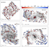 |
Fig. 9 Mapping electron temperatures within H ii regions across four of the PHANGS-MUSE galaxies (NGC 1672, NGC 1365, NGC 4254, and NGC 628). Coverage is not just limited to spiral arms, but samples the full inner star-forming disks in our sample of galaxies. NGC 1365 (Ho et al. 2017) and NGC 1672 (Kreckel et al. 2019; Ho et al. 2019) have both reported azimuthal abundance variations, with enhanced abundances along the spiral arms, which is supported by decreased Te along the eastern arms in both galaxies. The more flocculent galaxy NGC 4254 and the bar-free grand design spiral galaxy NGC 628 both show some tentative azimuthal trends, but the connection with spiral structure is more tenuous. Small-scale (<1 kpc) homogeneity in the temperature distribution is reminiscent of the trends for more uniform metallicity on small scales reported in Kreckel et al. (2020) for these targets. |
5 Results
We now apply the charge-exchange method to model Te within the full sample of 24 173 PHANGS-MUSE H ii regions.
5.1 Electron temperatures across thousands of H ii regions
We find that 4129 H ii regions meet the criteria outlined in Sect. 4.3, allowing us to compute Te for nearly a fifth of the H ii region sample. This is a factor of ~4 more H ii regions than have any auroral line detection, and a factor of ~8 more H ii regions than have direct detection of the [N ii] λ5755 line. The limiting factor for ~2000 of the regions is the requirement that the emission lines be detected with sufficient contrast against the surrounding DIG background, and for ~5000 H ii regions [S iii]/[S ii] is too low. Another ~5000 H ii regions meet neither criterion. The remaining ~7000 targets do not have sufficient S/N in all lines necessary.
With hundreds of measurements per galaxy, we show two-dimensional maps of Te across four example galaxies (Fig. 9). NGC 1672 and NGC 1365 both have previously identified azimuthal variations in their abundance distribution (Ho et al. 2017; Kreckel et al. 2019), as identified using strong line methods, with increased metallicities along the spiral arms. We similarly observe decreased Te in the H ii regions located along the spiral arm ridges, supporting that result (see also Ho et al. 2019), although the effect is less pronounced. NGC 4254 shows a much more flocculent spiral pattern, and the Te measurements more uniformly sample the disk. NGC 628 hosts a two arm spiral pattern without a bar or strong bulge component, and exhibits a clear gradient in Te with galactocentric radius.
Figure 10 quantifies the scatter in Te as a function of scale within all of our maps. Measuring the variation in Te across 500 pc or 3 kpc scales around each H ii region, relative to the mean local value at each position, we find that the probability density function reveals systematically smaller scatter on small physical scales. To perform this calculation, we considered the variation between neighboring regions only when 5 or more H ii regions are clustered on 500 pc or 3 kpc scales. We measure a standard deviation of ~500 K at 500 pc scales, and ~800 K at 3 kpc scales. To test the null hypothesis, that all regions temperatures are uncorrelated, we shuffled all values of Te and repeated this calculation (dotted lines). This test erases the trend with physical scale and results in a broader distribution. This small-scale homogeneity in the Te distribution reflects the spatial scales relevant to mixing, as also recently determined from strong line methods (Kreckel et al. 2020; Li et al. 2021; Metha et al. 2021; Williams et al. 2022).
In Fig. 11 we show the radial gradient in Te for each of the 19 galaxies. All galaxies show positive gradients, reflecting an expected negative metallicity gradient (Fig. 12), such as is typically observed across nearby galaxy samples (Pilyugin et al. 2014). In four galaxies (NGC 1300, NGC 1365, NGC 1566, and NGC 4535), significant (~900–1000 K) scatter is seen in these radial trends, in excess of the uncertainty intrinsic to the method (~600 K). This could be indicative of particularly large azimuthal abundance variations in these galaxies, which was also conclusively shown for two of these galaxies in interpolated metallicity maps (Williams et al. 2022).
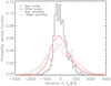 |
Fig. 10 Probability density function of the variations in Te at 500 pc (black) and 3 kpc (red), sampling scales across all galaxies in the sample. We performed this calculation around each H ii region, relative to the mean local value at each position. We required at least five H ii regions be located within the relevant sampling scale length to minimize biases due to low number statistics. Across all galaxies, we measure a standard deviation of ~500 K at 500 pc scales and ~800 K at 3 kpc scales. To test the null hypothesis, that all region temperatures are uncorrelated, we shuffled all values of Te and repeated this calculation (dotted lines). |
5.2 Why does this even work?
There are a few crucial assumptions that go into this model (see also Sect. 2). This model compares the [O i] and Hα line emission; however, considering the ionization structure within a nebula (Fig. 13), it is clear that these emission lines arise from different regions, with Hα emitted predominantly throughout the interior while [Ο i] is emitted mainly in an outer shell. For this work, we are assuming that Te is uniform across both the Hα and [Ο i] emitting regions, as is shown in our Cloudy modeling (orange line, Fig. 13). At sufficiently high spatial resolution, it would be possible to resolve the internal nebular structure and compare [Ο i] and Hα emission arising from the same parcel of gas, more directly ensuring that this assumption is true, but this is beyond what is possible given our ~50 pc physical resolution. This condition of uniform Te and co-spatial [Ο i] and Hα emission is also likely true in the diffuse ionized gas (e.g., Reynolds etal. 1998).
This method also assumes that the gas is photoionized, and contributions from shocks are negligible. The [Ο i]/Hα ratio is quite sensitive to shock excitation (Allen et al. 2008), spanning two orders of magnitude at constant metallicity and different shock velocities. Therefore, we expect the observed ratio of [Ο i]/Hα to change significantly in the presence of shocks. This is directly observed in supernova remnants (Kopsacheili et al. 2020), and in general we note that the observational locus of“star-forming regions” is not well represented by models in the [Ο i] BPT diagram (e.g., Law et al. 2021). How much of this discrepancy is due to the diffuse ionized gas (DIG), and the source of excitation for that diffuse emission, remains an active field of research (Belfiore et al. 2022). Our PHANGS-MUSE nebular catalog has attempted to minimize the impact of other ionizing sources by selecting peaks in Hα, using the BPT diagnostic cuts, and having a high contrast against the DIG. We further require our emission lines to be detected with 50% contrast against the DIG. Finally, we attempt to minimize the possibility of shock contributions by employing BPT diagnostic cuts, as described in Sect. 3.2.
Finally, an essential step in our method is our ability to infer fion in an independent way from the available strong lines. We find the strongest correlation with [S iii]/[S ii] (Fig. 1), a robust tracer of the ionization parameter. This begs the question of why the ionization fraction is related to the ionization parameter (q). Here we consider principally the incident ionization parameter, as seen by the inner edge of the nebula. By definition,  (Eq.13)), and
  (Eq. (4)). Assuming case B, Q(H0) could be expressed as Q(H0) ≃ αB ∫nen+dV, where αB is the recombination rate coefficient. Assuming a H ii region as a thin sphere (a common approximation), we can write that dV = 4πR2dl, where l is the thickness of the shell. Thus,
  , and we find that q ∝ fion at constant l and ne. However, we must keep in mind for this argument that this is fion measured over the full nebula, and not just over the [Ο i] region in the outer shell.
The remarkable success of this charge-exchange method for deriving Te in comparison with ~500 Η ii regions in the PHANGS-MUSE sample that have direct auroral line constraints (Fig. 7) demonstrates that the spatial averaging over the entire Η ii region does not invalidate this method. Crucially, as we show through more detailed Cloudy modeling in Sect. 5.3, this simplistic assumption does not seem to invalidate our derived dependence of fion on [S iii]/[S ii], but in fact appears to reduce the scatter in this relation.
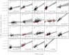 |
Fig. 11 Radial gradient in Te for each of the PHANGS-MUSE galaxies. Red points show Te determined from auroral line measurements, while black points show Te measured using the charge-exchange method. Positive slopes show general agreement with the expected flat to negative metallicity gradients reported in these and other nearby galaxies (Pilyugin et al. 2014; Kreckel et al. 2019). A linear fit is shown for each galaxy, with the fit parameters listed in the top of each plot. The gray band indicates the uncertainty in the linear fit, accounting for 600 Κ systematic uncertainty in the Te measurements. |
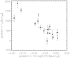 |
Fig. 12 Slope of the radial gradient in Te as a function of the slope of the radial gradient in 12+log(O/H) (Santoro et al. 2022) for each PHANGS-MUSE galaxy. Positive slopes in temperature correspond (as expected) to negative slopes in metallicity, as metal-rich gas is more efficient at cooling. |
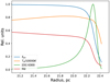 |
Fig. 13 Cloudy modeling of the interior structure of a typical H ii region. The Hα emission (red) traces fairly closely the ionization fraction (fion, blue) as a function of radius, while the [O i] (green) is predominantly emitted in the outer shell of the nebula. In this way, it is apparent that very little of the Hα emission is co-spatial with the [O i], a key assumption in our model. At the outer edge of the nebula, the intensity of [O i] rapidly drops together with the electron temperature Te (orange). |
5.3 Comparison of our flon relation with models
Crucial to the success of this technique is our ability to infer fion directly from the [S iii]/[S ii] line ratio. While we establish this empirically through comparison with the PHANGS-MUSE and CHAOS H ii regions (Sect. 4.2 and Fig. 6), we here explore how such a relation might emerge from theoretical models.
We compute a set of Cloudy models (Ferland et al. 2017) for the properties of ionizing clusters and nebulae covering the same parameter space as in the observed sample. To start, we crossmatch our catalog of PHANGS-MUSE H ii regions with measured auroral lines to a catalog of the stellar associations detected within PHANGS-Hubble Space Telescope (HST) imaging (Lee et al. 2022; Scheuermann et al., in prep.). These stellar associations have been identified using a watershed method applied to the near-UV and V-band images, and their key parameters (stellar mass, age, reddening) have been inferred from spectral energy distribution modeling (Larson et al., in prep.). We identify 150 objects with a one-to-one correspondence between an Η ii region and a stellar association, where we can be fairly certain that the identified stellar association is powering the ionization of the Η ii region. These 150 matched objects have a median age of ~3 Myr and a median stellar mass of ~104 M⊙, and we can further constrain properties such as size (R), gas-phase metallicity (12+log(O/H)), and electron density (ne), as shown in Fig. 14. This cross-matched sample was used to establish the range of model parameters that we explore.
We run Cloudy ν 17.02 models (using the PYCLOUDY package, Morisset 2013) consisting of a spherical gas cloud surrounding an ionizing source and take the following range in parameters based on the observations: constant density nH ≃ ne = 20, 90 and 300 cm”−3; metallicity 12 + log(O/H) = 7.99, 8.47 and 8.69 (that corresponds to Ζ/ΖΘ = 0.2, 0.6 and 1.0 assuming the Solar relative abundance of elements from Grevesse et al. 2010); inner radius of the shell R = 0 (cloud), 15, 28, 40 pc. We also varied the volume filling factor in the range 0.1 – 1.0, but it has a neglectable effect on the output models. As an ionizing source we used the spectra produced by Starburst99 (Leitherer et al. 2014) for instantaneous star formation, a Kroupa initial mass function (Kroupa 2001), and Geneva stellar evolution tracks, which include rotation (metallicity Ζ = 0.014, Ekström et al. 2012, and Ζ = 0.002, Georgy et al. 2013)1 for clusters with total stellar mass log(M*/M⊙) = (3.5, 4.5, 5.5) and ages of 0.6 Myr plus 1 to 9 Myr with steps of 1 Myr. Each Cloudy model has been iterated until convergence, and the termination criterium was reaching the lowest temperature Te= 4000 K. We can then compute integrated properties across the full model, including line fluxes, line ratios, and fion. As follows from the bottom-right panel of Fig. 14, the resulting grid of Cloudy and Starburst99 models produces the same range of Hα luminosities as that seen for the reference H ii regions selected from PHANGS-MUSE; however, the exact distributions do not match each other because the model parameter space is regularly sampled (in contrast to the observational data).
We derive the integrated value of fion from the Cloudy models as the ratio of number densities averaged over a nebula volume:
 (16)
(16)
where nH+(r) and nH(r) are the ionized and total hydrogen number density in each zone of the modeled nebula, and r is the radius of the corresponding zone. We can easily calculate these integrals from the computed Cloudy models and thus obtain fion characterizing the whole nebula.
As seen in the left-hand panel of Fig. 15, the range of values for fion calculated in the models agrees very well with the measurements obtained from observations, but with large scatter. This scatter in the fion relation as a function of [S iii]/[S ii] is significantly larger than in the observational measurements, driven mostly by differences in the age of the ionizing cluster. To some extent, the reduced scatter for the observational data could be a result of an observational bias, as many of the stellar associations have very young ages (~1 Myr; Fig. 14). However, we see clear offsets between the youngest Cloudy models and the empirical relation derived in Fig. 6. We also note that a similar correlation between fion and [S iii]/[S ii] exists also at the scales of individual zones (radii) of the models (central panel) where fion is not affected by the truncation criteria of a model or by its geometry.
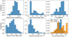 |
Fig. 14 Distributions of the observed properties for 150 Η ii regions with measured auroral lines and a one-to-one correspondence with a young stellar association (Scheuermann et al., in prep.). These ranges in cluster mass, stellar cluster age, gas-phase metallicity, size and electron density are used to establish the parameter range used in our Cloudy models. Bottom-right panel: distribution of the reddening-corrected Hα luminosity in both the observational sample and computed Cloudy models. |
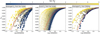 |
Fig. 15 Relation between fion and [S iii]/[S ii] based on the Cloudy models. On the left-hand panel the value of fion is obtained directly from the model (as < n(H+) > / < n(H) >), while on the right-hand panel it was derived as in the observations (Eq. (6)) based on the integrated values of [Ο i]/Ηα metallicity and electron temperature Te([N ii]). Central panel: fion = n(H+)/n(H) in individual zones of the models. The colors on all panels correspond to the age of the ionizing cluster, and the red curve is the empirical relation derived from the observational data (Eq. (15)). Spatially integrating across the entire line emitting region clearly reduces the scatter in this relation, and brings the model results into better agreement with the empirical relation. |
5.3.1 Assumption of co-spatial [O i] and Hα
One of the limitation of the charge-exchange method (as described in Sect. 5.2) is that Eq. (6) should only work for [O i] and Hα emitted co-spatially within a nebula, but in unresolved observations we collect line emission from the whole nebula. Thus, our measurement of [Ο i]/Hα differs from the value corresponding to the area where the charge-exchange process occurs. This, in turn, should lead to deviations between the fion empirically calibrated for this work and fion when considering only the [Ο i] emitting region. From our Cloudy models, we directly estimate how significant this deviation is. For that we calculate fion following the method used with our observational data -we measure the integrated value of [Ο i]/Hα, adopt the input metallicity of the model, and derive fion using Eq. (6) assuming Te=Te([N ii]) as obtained directly from the model. In Fig. 15 (right) we show that the discrepancy between the empirical correlation and the Cloudy models is significantly reduced when we calculate fion in the same way as we did with the observational data. We note in particular that the scatter in fion versus [S m]/[S ii] is very similar to that for observational data, and now the empirical relation correlates with the Cloudy models for youngest age (see the right-hand panel of Fig. 15), consistent with the expected observational bias.
The fact that the“true” values of fion do not agree with those obtained from Eq. (6) directly follows from the limitation of this equation when applied to unresolved H ii regions. Indeed, we can invert our use of Eq. (6), and use it to compute the expected [Ο i]/Hα based on our Cloudy models. The values of [Ο i]/Ha that we compute from Eq. (6) assuming the true fion derived from Eq. (16) are significantly overestimated in comparison with the true line ratios from the Cloudy models (left-hand panel of Fig. 16). At the same time, Eq. (6) reproduces well the [Ο i]/Ha ratio when it is applied to the individual local zones of the Cloudy models (central panel of Fig. 16)2. We show in Appendix A that a revised version of Eq. (6) that considers the volumetric differences in the [O i] and Hα emitting zones is more complicated (Eq. (A.23)) and cannot be solved for unresolved H ii regions. However, we can test the impact introducing a volumetric correction using the Cloudy models. Integrating the term ξ, dependent on the local fion over all Cloudy zones, we obtain values for [Ο i]/Hα that are in very good agreement with those in the output of the Cloudy models (right-hand panel of Fig. 16).
From this analysis we conclude that Eq. (6), which is fundamental to our method, is valid for both resolved and unresolved nebulae, but for the latter it is necessary to weigh fion according to the volumes occupied by the [Ο i] and Hα emitting zones instead of using the true fion. By definition, the values of fion derived from [Ο i]/Hα and used in the right-hand plot of Fig. 15 already include these weights, and that is why they disagree with the true fion (Fig. 16, left). The empirically defined values of fion obtained by Eq. (15) are weighted as the ionization structure in sulfur encodes some of these volumetric effects, and as a result our relation intrinsically corrects for this potential bias.
As the goal of the presented method is to obtain the measurements of electron temperature, we carry out a final test by comparing the values of Te([N ii] derived from Eq. (6)) with the output of our Cloudy models. As follows from Fig. 17, in general, both values are indeed in agreement if we use the observation-ally defined calibration of fion (Eq. (15)), or solve Eq. (A.23) on a zone-by-zone basis. Moreover, the empirical calibration shows even better agreement with the one-to-one relation in the high Te regime. We note, however, that the method significantly underestimates Te for the regions ionized by older star clusters. In summary, while we have shown the theoretical limitations of this approach, based on the underlying physical mechanisms governing the charge-exchange process, we further demonstrate that our empirical calibration based on integrated nebulae sufficiently accounts for the unresolved volumetric effects.
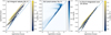 |
Fig. 16 Validation of Eq. (6) using our Cloudy models. Panel α: comparison of [Ο i]/Ηα calculated with this relation assuming the mean fion (Eq. (16)) to the Cloudy output. Panel b: same comparison, but applied to the individual local zones in the Cloudy models. Here fion corresponds to the local values of n(H+)/n(H). Panel c: same test, but applied to results using Eq. (A.23) that are accounting for variations of fion and the spatial extent of the [O i] and Hα emitting zones. |
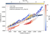 |
Fig. 17 Validation of the resulting values for Te based on the Cloudy models. Crosses shows the values of Te([N ii]) obtained from the volumetric version of Eq. (6), which accounts for variations in fion and the spatial extent of the [O i] and Hα emitting zones (Eq. (A.23)). Circles represent the Te([N ii]) values yielded by Eq. (6) assuming the empirical calibration of fion (by Eq. (15)). The calculated values are compared with the“true” Te([N ii]) from the Cloudy models. The symbol color encodes the age of the ionizing cluster. Both data sets show generally good agreement with the one-to-one relation, but the empirical calibration significantly underestimate Te for old regions. We note that for the empirically calibrated results we show only the models with log([OI]/Hα) ≥ -3 and -1 ≥ log([SIII]/[SII]) ≤ −0.7 that correspond to the values obtained in our observations (see, e.g., Figs. 3 and 6). The prominent“tails” toward higher Te for the empirically calibrated values correspond only to those regions where log([SIII]/[SII]) > 0.5. Only a few such regions were used for calibration of Eq. (15), and thus the calibration is less certain for Η ii regions with the highest ionization parameters. |
5.3.2 Age as a secondary parameter
Based on the remarkable visual agreement between the Cloudy models and observed data when using fion inferred from [Ο i]/Hα in the models, and the matched biases regarding spatial averaging, we chose to use this modeled value of fion to independently derive a relation between fion and [S iii]/[S ii]. We apply our empirical calibration from Eq. (15) to the Cloudy models. As shown in Fig. 18 (left), this relation shows relatively good agree-ment at high fion > 0.9, but a clear secondary dependence on age. While the age of an Hll region is difficult to constrain observationally, strong correlations are seen in models with the equivalent width (EW) of Hα (Leitherer et al. 2014). We use the EW output from the Cloudy models, and include this secondary dependence to perform a third order polynomial fit to Fig. 15 (right) in order to derive the following functional form:
 (17)
(17)
where again χ = log10([S iii]/[S ii]) and y = log10(EW(Hα)). In Fig. 18 (right), we see that this successfully removes the secondary dependence on age.
There is one remaining complication in our comparison of the modeled and observed empirical relations. According to the Cloudy models, we find that EW(Hα) ≈ 1815 Å at an age of 1 Myr; however, based on our observations, we find EW(Hα) ≈ 126 Å for the same aged nebulae that show a one-to-one correspondence with the HST stellar associations (Larsen et al., in prep.; Scheuermann et al., in prep.). This offset between modeled and observed EW has been previously reported (Morisset et al. 2016), and it can be a consequence of the large escape fraction of ionizing radiation from H ii regions, or of the significant contribution of underlying old stellar population – both factors are not considered in the Cloudy models. Likely we are seeing a combination of both effects, as typical escape fractions are expected to be ~50% (Oey & Kennicutt 1997; Doran et al. 2013; Belfiore et al. 2022), which alone is insufficient to account for the difference. To first order a simple scaling is possible whereby we “convert” the observed EW(Hα) to the modeled EW(Hα) at this fixed reference age of 1 Myr, such that the variable y in Eq. (17) is replaced with y = log10(EW(Hα)obs. 1815/126).
We applied this prescription to the PHANGS-MUSE H ii region catalog and show the resulting values in Fig. B.1. Directly comparing the EW(Hα) measurements with the Cloudy derived model for fion (Fig. 19), it is apparent that while the general trends are in agreement, the exact values of EW(Hα) between the models and observations are not in good enough agreement that we can rely on the calibration. However, it demonstrates the potential in future work for improving our Te measurements by including age sensitive indicators (such as EW(Hα)) in the prescription, which is not generally done in the literature.
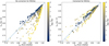 |
Fig. 18 Comparison of the cloudy modeled fion measured from [Ο i]/Ηα with what is derived using a fit based on [S iii]/[S ii] (as in Fig. 15, right). Left-hand panel: depends only on x = log10([S iii]/[S ii]) while the right-hand panel includes a secondary dependence on age as traced by the EW of Hα, as y = log10(EW(Hα)). Both plots are colored by the age of the ionizing stellar cluster, and correcting for this secondary dependence on age significantly improves the agreements between the fit and the value for fion in the cloudy models. |
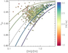 |
Fig. 19 Direct comparison of the observed fion as a function of [S iii]/[S ii] within the PHANGS-MUSE Η ii regions with the age-dependent fit resulting from the cloudy models (colored lines, Eq. (17)). The colors correspond to EW(Hα), and for the cloudy model fits they have been scaled as described in the text in order to account for the large quantitative discrepancy between model and observation. The observed data shows a clear gradient, indicating that age trends do play an important role in driving the scatter in this relation. The empirical fit (dashed line) shows good qualitative agreement with the age-dependent cloudy model fit, supporting our choice of this empirical calibration. However, while the trends are consistent, a significant offset is seen between the EW(Hα) measurements and the predicted values, preventing a straightforward application of our model-driven calibrations to the data. |
6 Conclusions
We have developed a new method that exploits the charge exchange between oxygen and hydrogen to infer the electron temperature, Te, within H ii regions using only strong emission lines. This single temperature corresponds to the [O i] and Hα emitting zone. This method requires three parameters: the [Ο i]/Hα line ratio, the gas-phase metallicity 12+log(O/H), and the ionization fraction, fion. Using observations from the CHAOS survey (Berg et al. 2020), where auroral line observations of Te are available for ~ 150 H ii regions, we demonstrate that fion correlates with changes in various strong line ratios. We show that the strongest correlation is with [S iii]/[S ii], tracing changes in the ionization parameter. However, due to aperture biases, we cannot derive an empirical relation from this data set alone.
We then used 840 H ii regions from the PHANGS-MUSE survey that have auroral line detections of [N ii] λ5755 to develop an empirical relation between fion and [S iii]/[S ii] for line fluxes measured across integrated H ii regions. Due to limitations of our calibration sample and concerns about the contribution from diffuse ionized gas, where strong lines such as [S ii] and [O i] are strongly emitted, we conservatively applied this method only to H ii regions that have [S iii]/[S ii] > 0.5 and a contrast of more than 50% against the local DIG background. With these restrictions, we recover Te([N ii]) to within ~600 K. This uncertainty only increases slightly when we assume a fixed metallicity for each galaxy, demonstrating that this charge-exchange method is not strongly sensitive to the exact determination of metallicity.
Of the ~24 000 H ii regions in the PHANGS-MUSE nebular catalog (Santoro et al. 2022), we were then able to apply this technique to model Te for a total of 4129 H ii regions, ~4 times more than have direct auroral line detections. We recover positive radial temperature gradients that reflect the expected negative metallicity gradients. Four galaxies show a scatter in their radial temperature gradient of ~1000 K, well beyond the uncertainties of the method and which likely trace azimuthal variations in the metallicity at fixed radius.
While some of the assumptions that go into this method would not appear to be met, particularly the assumption that the [O i] and Hα emitting regions have matched electron temperatures, and ideally are co-spatial, we carried out a set of Cloudy models to explore the robustness of our method and in particular to test the empirically derived relation between fion and [S iii]/[S ii]. We find that by integrating over the full H ii region, our models actually recover the tight observed correlation between fion and [S iii]/[S ii], with a significant secondary dependence on the age of the ionizing stellar cluster. We parameterize this age dependence by changes in the EW of Hα, which shows qualitatively similar agreement to the observed data but significant quantitative differences in the measured values, particularly for EW(Hα). For this reason, we prefer the empirical calibration for fion, but we note that age/EW(Hα) represents a promising additional parameter to consider when deriving accurate H ii region temperatures and metallicities.
This novel method for determining Te demonstrates the remarkable potential arising from new catalogs that contain hundreds to thousands of H ii regions with uniform data, as well as future planed surveys such as SIGNALS (Rousseau-Nepton et al. 2019), SDSS-V/LVM (Kollmeier et al. 2017), and AMASE (Yan et al. 2020). While this method is physically motivated, there is clearly an exciting potential for the application of machine learning approaches to these data sets.
Acknowledgements
We thank the referee for their comments, which improved our analysis of the subtleties of this method. We thank Jose Eduardo Mendez Delgado for his comments and input. This work was carried out as part of the PHANGS collaboration. Based on observations collected at the European Southern Observatory under ESO programmes 1100.B-0651, 095.C-0473, and 094.C-0623 (PHANGS-MUSE; PI Schinnerer), as well as 094.B-0321 (MAG-NUM; PI: Marconi), 099.B-0242, 0100.B-0116, 098.B-0551 (MAD; PI: Carollo) and 097.B-0640 (TIMER; PI: Gadotti). K.K., O.V.E. and F.S. gratefully acknowledge funding from the German Research Foundation (DFG) in the form of an Emmy Noether Research Group (grant number KR4598/2-1, PI: Kreckel). S.C.O.G. and R.S.K. acknowledge support from the DFG via SFB 881 “The Milky Way System” (Project-ID 138713538; sub-projects B1, B2 and B8) and from the Heidelberg cluster of excellence EXC 2181-390900948 “STRUCTURES: a unifying approach to emergent phenomena in the physical world, mathematics, and complex data”, funded by the German Excellence Strategy. R.S.K. furthermore thanks for funding from the European Research Council via the ERC Synergy Grant ECOGAL (grant 855130). T.G.W. acknowledges funding from the European Research Council (ERC) under the European Union’s Horizon 2020 research and innovation programme (grant agreement No. 694343). F.B. would like to acknowledge funding from the European Research Council (ERC) under the European Union’s Horizon 2020 research and innovation programme (grant agreement No.726384/Empire).
Appendix A Derivation of line emissivity relation
The emissivity of [O i] λ6300 transition can be written as:
 (A.1)
(A.1)
where ROI is the excitation rate coefficient for the 3P−1D transition and δΕOΙ is the energy of the transition. If we assume that the electrons come primarily from ionized hydrogen, then n(e−) ≃ n(H+) and we can instead write this as
 (A.2)
(A.2)
The Hα emissivity due to H+ recombination can be written as
 (A.3)
(A.3)
where Rα is the rate coefficient for the production of Hα photons during recombination (i.e., the product of the recombination rate and the fraction of recombinations resulting in Hα) and δεΗα is the energy of Hα. Taking the ratio of the emissivities yields
 (A.4)
(A.4)
We now want to eliminate the dependence on the O0 fraction in favor of a dependence on the H+/H ratio and the total elemental abundance of oxygen To do this, we use the fact that the balance between O0 and O+ is set by charge transfer with hydrogen:
 (A.5)
(A.5)
 (A.6)
(A.6)
If we denote the rate coefficient for the forward reaction (producing O+) as kf and the rate coefficient for the reverse reaction as kr, then chemical equilibrium between these two reactions implies that
 (A.7)
(A.7)
Denoting the total elemental abundance of oxygen as n(o), we can use the relation n(O+) = n(O) − n(O0) to write this as
![Mathematical equation: ${k_{\rm{f}}}n\left( {{{\rm{O}}^0}} \right)n\left( {{{\rm{H}}^ + }} \right) = {k_{\rm{r}}}\left[ {n\left( {\rm{O}} \right) - n\left( {{{\rm{O}}^{\rm{0}}}} \right)} \right]n\left( {{{\rm{H}}^0}} \right).$](/articles/aa/full_html/2022/11/aa43858-22/aa43858-22-eq28.png) (A.8)
(A.8)
Rearranging for n(O0) then yields
![Mathematical equation: $n\left( {{{\rm{O}}^0}} \right) = n\left( {\rm{O}} \right)n\left( {{{\rm{H}}^0}} \right){\left[ {{{{k_{\rm{f}}}} \over {{k_{\rm{r}}}}}n\left( {{{\rm{H}}^ + }} \right) + n\left( {{{\rm{H}}^0}} \right)} \right]^{ - 1}}.$](/articles/aa/full_html/2022/11/aa43858-22/aa43858-22-eq29.png) (A.9)
(A.9)
The difference between the ionization potentials of hydrogen and oxygen is very small and at high temperatures we can ignore it and assume that the energy change in the forward and reverse reactions is zero. In this case, the ratio of the forward and reverse rate coefficients is simply the ratio of the statistical weights of the products:
 (A.10)
With  and
and  , this yields kf /kr = 8/9. Therefore,
![Mathematical equation: $n\left( {{{\rm{O}}^0}} \right) = n\left( {\rm{O}} \right)n\left( {{{\rm{H}}^0}} \right){\left[ {{8 \over 9}n\left( {{{\rm{H}}^ + }} \right) + n\left( {{{\rm{H}}^0}} \right)} \right]^{ - 1}},$](/articles/aa/full_html/2022/11/aa43858-22/aa43858-22-eq33.png) (A.11)
(A.11)
![Mathematical equation: $ = n\left( {\rm{O}} \right)r\left[ {{8 \over 9} + r} \right]^{- 1} $](/articles/aa/full_html/2022/11/aa43858-22/aa43858-22-eq34.png) (A.12)
(A.12)
where r = n(H0)/n(H+). Substituting this into the ratio of the emissivities then yields
 (A.13)
Finally, we can use the fact that
![Mathematical equation: $n\left( {\rm{H}} \right) = n\left( {{{\rm{H}}^{\rm{ + }}}} \right) + n\left( {{{\rm{H}}^{\rm{0}}}} \right) = n\left( {{{\rm{H}}^{\rm{ + }}}} \right)[1 + r]$](/articles/aa/full_html/2022/11/aa43858-22/aa43858-22-eq36.png) (A.14)
(A.14)
to write this as
 (A.15)
where ξ = (1 + r)/(8/9 + r). Comparing this with Equation 1 in Reynolds et al. (1998) shows us that they use the following expression for  :
:
 (A.16)
where T4 = T/10000 K.
For our updated calculation, we computed ROI for large number of different temperatures by numerically integrating the cross-section data3 from Barklem (2007) and have then fit a function to the resulting rate. The best fit that we have found is the following:
 (A.17)
where
 (A.18)
This fit is accurate to within 3% for temperatures in the range 3000 < T < 30000 K, but is not guaranteed to give sensible results outside of this temperature range.
Since ΔΕOI = 3.155 × 10⁻¹², it then follows that
 (A.19)
For Hα, we can use the accurate fit given in Draine (2011) to the data of Hummer & Storey (1987):
 (A.20)
This fit is also accurate to within a few percent in the temperature range of interest. Combining these then yields
 (A.21)
and hence
 (A.22)
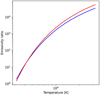 |
Fig. A.1 Comparison of the emissivity coefficients computed in Section A (red) with the value provided in Reynolds et al. (1998) (blue). For H ii region temperatures in the normal range for PHANGS galaxies, the difference is around 20–40%. |
A comparison of the relations for  provided by Reynolds et al (1998) and derived here is shown in Figure A.1
We note that, in general, the ratio of the total observed fluxes in [O i] and Hα is not equal to the ratio of their emissivities, but can be expressed from the equations above as follows (assuming a uniform Te across the [O i] and Hα emitting zones):
![Mathematical equation: $\matrix{{I\left( {\left[ {{\rm{OI}}} \right]} \right)/I\left( {{\rm{H}}\alpha } \right)} \hfill & = \hfill & {{{\int_{V\left[ {{\rm{OI}}} \right]} {{ \in _{{\rm{OI}}}}dV} } \over {\int_{{V_{{\rm{H}}\alpha }}} {{ \in _{{\rm{H}}\alpha }}dV} }} = } \hfill \cr {} \hfill & = \hfill & {8492{{{f_{{\rm{OI}}}}\left( T \right)} \over {T_4^{ - 0.942 - 0.031\ln {T_4}}}}\exp \left( { - {{2.284} \over {{T_4}}}} \right)\xi '{{n\left( {\rm{O}} \right)} \over {n\left( {\rm{H}} \right)}}} \hfill \cr } , $](/articles/aa/full_html/2022/11/aa43858-22/aa43858-22-eq47.png) (A.23)
(A.23)
where ξ′ depends on the distribution of the hydrogen ionization fraction fion = n(H+)/n(H) = 1/(1 + r) in the [O i] and Hα emitting zones as
![Mathematical equation: $\xi ' = {{\int_{{V_{\left[ {OI} \right]}}} {{r \over {\left( {1 + r} \right)\left( {8/9 + r} \right)}}dV} } \over {\int_{{V_{H\alpha }}} {1/{{\left( {1 + r} \right)}^2}dV} }}.$](/articles/aa/full_html/2022/11/aa43858-22/aa43858-22-eq48.png) (A.24)
(A.24)
Equation (A.23) is equal to Equation A.22 (and thus - to Equation 6) if one assumes that [O i] and Hα come from the same zones. We discuss the limitation of this assumption in Section 5.3.1.
Appendix B Application of the model-based prescription for fion
As described in Section 5.3, we use a series of Cloudy models to derive fion as a function of [S iii]/[S ii] across integrated H ii regions. Given the similarities between the model results and our observations, we explore using the Cloudy models to derive a new prescription for fion, and improve upon them by adding an age dependence based on variations in EW(Hα) (Equation 17).
In this section, we explore how well this model-driven parameterization of fion applies to our observed PHANGS-MUSE H ii regions. For each H ii region, we calculate EW(Hα) to use as an age tracer. Here, we assume that the stellar continuum is dominated by light from the young stellar population, which may not be the case for low EW(Hα) regions. Given the added dependence on age (via inclusion of EW(Hα)), we can remove our requirement that [S iii]/[S ii] > 0.5. We find that this doubles the number of H ii regions for which we can apply the charge-exchange method to a total of ~9000 H ii regions, nearly half of all H ii regions in the PHANGS-MUSE sample.
In Figure B.1 we compare the charge-exchange method Te with the Te derived from auroral line detections. We note that the scatter is significantly increased (~1000 K instead of 600 K). Considering only H ii regions with EW(Hα) > 50 A significantly reduces this scatter but also limits the total number of H ii regions.
In Figure B.2 we plot the radial gradient in Te for each galaxy. Again, we see that for many of the H ii regions at low EW(Hα) this prescription for fion results in particularly large Te values (10 000–12 000 K).
As this revised parameterization for fion does not result in improved agreement with Te([N ii]) and results in unphysically high Te values along the radial gradient, combined with the systematic offsets between modeled and measured EW(Hα), we choose in this paper to adopt the empirically calibrated relation for fion(Equation 15).
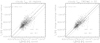 |
Fig. B.1 Comparison of Te derived from the charge-exchange method, with Te([N ii]), derived from auroral line detections, for Η ii regions in the PHANGS-MUSE sample. For the charge-exchange method, we use the parametrization of fion derived from Cloudy models (Equation 17). We find systematically larger scatter (~1000 K) compared to the relation in Figure 7, where fion was empirically calibrated. The scatter is still larger, even when we only consider younger (higher EW(Hα)) Η ii regions. |
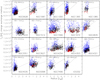 |
Fig. B.2 Radial gradients in Te for each galaxy, using fion parameterized from Cloudy models (Equation 17). Η ii regions marked in blue have EW(Hα)<50 Å a regime poorly sampled by our calibrations and at the extremes of the Cloudy models. These all have systematically higher Te, suggesting problems with the calibration. Η ii regions with younger ages (black) show better agreement with the auroral line measurements (red), similar to Figure 11. |
References
- Allen, M. G., Groves, B. A., Dopita, M. A., Sutherland, R. S., & Kewley, L. J. 2008, ApJS, 178, 20 [Google Scholar]
- Anand, G. S., Lee, J. C., Van Dyk, S. D., et al. 2021, MNRAS, 501, 3621 [Google Scholar]
- Azimlu, M., Marciniak, R., & Barmby, P. 2011, AJ, 142, 139 [Google Scholar]
- Bacon, R., et al. 2010, Proc. SPIE, 7735, 773508 [NASA ADS] [CrossRef] [Google Scholar]
- Baldwin, J. A., Phillips, M. M., & Terlevich, R. 1981, PASP, 93, 5 [Google Scholar]
- Balser, D. S., Wenger, T. V., Anderson, L. D., & Bania, T. M. 2015, ApJ, 806, 199 [NASA ADS] [CrossRef] [Google Scholar]
- Barklem, P. S. 2007, A&A, 462, 781 [NASA ADS] [CrossRef] [EDP Sciences] [Google Scholar]
- Barnes, A. T., Glover, S. C. O., Kreckel, K., et al. 2021, MNRAS, 508, 5362 [NASA ADS] [CrossRef] [Google Scholar]
- Belfiore, F., Santoro, F., Groves, B., et al. 2022, A&A, 659, A26 [NASA ADS] [CrossRef] [EDP Sciences] [Google Scholar]
- Berg, D. A., Skillman, E. D., Croxall, K. V., et al. 2015, ApJ, 806, 16 [NASA ADS] [CrossRef] [Google Scholar]
- Berg, D. A., Pogge, R. W., Skillman, E. D., et al. 2020, ApJ, 893, 96 [NASA ADS] [CrossRef] [Google Scholar]
- Croxall, K. V., Pogge, R.W., Berg, D. A., Skillman, E. D., & Moustakas, J. 2015, ApJ, 808, 42 [NASA ADS] [CrossRef] [Google Scholar]
- Croxall, K. V., Pogge, R.W., Berg, D. A., Skillman, E. D., & Moustakas, J. 2016, ApJ, 830, 4 [NASA ADS] [CrossRef] [Google Scholar]
- Dong, R., & Draine, B. T. 2011, ApJ, 727, 35 [NASA ADS] [CrossRef] [Google Scholar]
- Dopita, M. A., Kewley, L. J., Sutherland, R. S., & Nicholls, D. C. 2016, Ap&SS, 361, 61 [NASA ADS] [CrossRef] [Google Scholar]
- Doran, E. I., Crowther, P. A., de Koter, A., et al. 2013, A&A, 558, A134 [NASA ADS] [CrossRef] [EDP Sciences] [Google Scholar]
- Dors, O. L., Jr., Krabbe, A., Hägele, G. F., & Pérez-Montero, E. 2011, MNRAS, 415, 3616 [NASA ADS] [CrossRef] [Google Scholar]
- Draine, B. T. 2011, Physics of the Interstellar and Intergalactic Medium (Princeton: Princeton University Press) [Google Scholar]
- Ekström, S., Georgy, C., Eggenberger, P., et al. 2012, A&A, 537, A146 [Google Scholar]
- Emsellem, E., Schinnerer, E., Santoro, F., et al. 2022, A&A, 659, A191 [NASA ADS] [CrossRef] [EDP Sciences] [Google Scholar]
- Ferland, G. J., Chatzikos, M., Guzmán, F., et al. 2017, Rev. Mex. Astron. Astrofis., 53, 385 [NASA ADS] [Google Scholar]
- Georgy, C., Ekström, S., Eggenberger, P., et al. 2013, A&A, 558, A103 [NASA ADS] [CrossRef] [EDP Sciences] [Google Scholar]
- Grevesse, N., Asplund, M., Sauval, A. J., & Scott, P. 2010, Ap&SS, 328, 179 [Google Scholar]
- Hausen, N. R., Reynolds, R. J., & Haffner, L. M. 2002, AJ, 124, 3336 [NASA ADS] [CrossRef] [Google Scholar]
- Ho, I. T. 2019, MNRAS, 485, 3569 [NASA ADS] [CrossRef] [Google Scholar]
- Ho, I. T., Seibert, M., Meidt, S. E., et al. 2017, ApJ, 846, 39 [NASA ADS] [CrossRef] [Google Scholar]
- Ho, I. T., Kreckel, K., Meidt, S. E., et al. 2019, ApJ, 885, L31 [NASA ADS] [CrossRef] [Google Scholar]
- Hummer, D. G., & Storey, P. J. 1987, MNRAS, 224, 801 [NASA ADS] [CrossRef] [Google Scholar]
- Kauffmann, G., Heckman, T. M., Tremonti, C., et al. 2003, MNRAS, 346, 1055 [Google Scholar]
- Kepley, A. A., Chomiuk, L., Johnson, K. E., et al. 2011, ApJ, 739, L24 [CrossRef] [Google Scholar]
- Kewley, L. J., & Dopita, M. A. 2002, ApJS, 142, 35 [Google Scholar]
- Kewley, L. J., & Ellison, S. L. 2008, ApJ, 681, 1183 [Google Scholar]
- Kewley, L. J., Heisler, C. A., Dopita, M. A., & Lumsden, S. 2001, ApJS, 132, 37 [Google Scholar]
- Kewley, L. J., Nicholls, D. C., & Sutherland, R. S. 2019, ARA&A, 57, 511 [Google Scholar]
- Klessen, R. S., & Glover, S. C. O. 2016, Saas-Fee Adv. Course, 43, 85 [NASA ADS] [CrossRef] [Google Scholar]
- Kollmeier, J. A., Zasowski, G., Rix, H.-W., et al. 2017, ArXiv e-prints [arXiv:1711.03234] [Google Scholar]
- Kopsacheili, M., Zezas, A., & Leonidaki, I. 2020, MNRAS, 491, 889 [CrossRef] [Google Scholar]
- Kreckel, K., Ho, I. T., Blanc, G. A., et al. 2019, ApJ, 887, 80 [NASA ADS] [CrossRef] [Google Scholar]
- Kreckel, K., Ho, I. T., Blanc, G. A., et al. 2020, MNRAS, 499, 193 [NASA ADS] [CrossRef] [Google Scholar]
- Kroupa, P. 2001, MNRAS, 322, 231 [NASA ADS] [CrossRef] [Google Scholar]
- Lang, P., Meidt, S. E., Rosolowsky, E., et al. 2020, ApJ, 897, 122 [CrossRef] [Google Scholar]
- Law, D. R., Ji, X., Belfiore, F., et al. 2021, ApJ, 915, 35 [NASA ADS] [CrossRef] [Google Scholar]
- Lee, J. C., Whitmore, B. C., Thilker, D. A., et al. 2022, ApJS, 258, 10 [NASA ADS] [CrossRef] [Google Scholar]
- Leitherer, C., Ekström, S., Meynet, G., et al. 2014, ApJS, 212, 14 [Google Scholar]
- Leroy, A. K., Schinnerer, E., Hughes, A., et al. 2021, ApJS, 257, 43 [NASA ADS] [CrossRef] [Google Scholar]
- Li, Z., Krumholz, M. R., Wisnioski, E., et al. 2021, MNRAS, 504, 5496 [NASA ADS] [CrossRef] [Google Scholar]
- Luisi, M., Anderson, L. D., Bania, T. M., et al. 2018, PASP, 130, 084101 [NASA ADS] [CrossRef] [Google Scholar]
- Luridiana, V., Morisset, C., & Shaw, R. A. 2015, A&A, 573, A42 [NASA ADS] [CrossRef] [EDP Sciences] [Google Scholar]
- Maiolino, R., & Mannucci, F. 2019, A&ARv, 27, 3 [Google Scholar]
- Mannucci, F., Belfiore, F., Curti, M., et al. 2021, MNRAS, 508, 1582 [NASA ADS] [CrossRef] [Google Scholar]
- McKee, C. F., & Ostriker, E. C. 2007, ARA&A, 45, 565 [Google Scholar]
- Metha, B., Trenti, M., & Chu, T. 2021, MNRAS, 508, 489 [NASA ADS] [CrossRef] [Google Scholar]
- Mingozzi, M., Belfiore, F., Cresci, G., et al. 2020, A&A, 636, A42 [NASA ADS] [CrossRef] [EDP Sciences] [Google Scholar]
- Morisset, C. 2013, Pycloudy: Tools to manage astronomical Cloudy photoionization code [record ascl:1304.020] [Google Scholar]
- Morisset, C., Delgado-Inglada, G., Sánchez, S. F., et al. 2016, A&A, 594, A37 [NASA ADS] [CrossRef] [EDP Sciences] [Google Scholar]
- Oey, M. S., & Kennicutt, R. C. J., 1997, MNRAS, 291, 827 [NASA ADS] [CrossRef] [Google Scholar]
- Osterbrock, D. E., & Ferland, G. J. 2006, Astrophysics Gaseous Nebulae and Active Galactic Nuclei (USA: University Science Books) [Google Scholar]
- Pilyugin, L. S., & Grebel, E. K. 2016, MNRAS, 457, 3678 [NASA ADS] [CrossRef] [Google Scholar]
- Pilyugin, L. S., Grebel, E. K., & Kniazev, A. Y. 2014, AJ, 147, 131 [NASA ADS] [CrossRef] [Google Scholar]
- Pineda, J. L., Horiuchi, S., Anderson, L. D., et al. 2019, ApJ, 886, 1 [NASA ADS] [CrossRef] [Google Scholar]
- Pogge, R. W., Atwood, B., Brewer, D. F., et al. 2010, SPIE Conf. Ser., 7735, 77350A [Google Scholar]
- Reynolds, R. J., Hausen, N. R., Tufte, S. L., & Haffner, L. M. 1998, ApJ, 494, L99 [NASA ADS] [CrossRef] [Google Scholar]
- Rosolowsky, E., & Simon, J. D. 2008, ApJ, 675, 1213 [NASA ADS] [CrossRef] [Google Scholar]
- Rousseau-Nepton, L., Martin, R. P., Robert, C., et al. 2019, MNRAS, 489, 5530 [NASA ADS] [CrossRef] [Google Scholar]
- Sánchez-Menguiano, L., Sánchez Almeida, J., Muñoz-Tuñón, C., et al. 2019, ApJ, 882, 9 [CrossRef] [Google Scholar]
- Santoro, F., Kreckel, K., Belfiore, F., et al. 2022, A&A, 658, A188 [NASA ADS] [CrossRef] [EDP Sciences] [Google Scholar]
- Schlafly, E. F., & Finkbeiner, D. P. 2011, ApJ, 737, 103 [Google Scholar]
- Tayal, S. S., Zatsarinny, O., & Sossah, A. M. 2019, ApJS, 242, 9 [NASA ADS] [CrossRef] [Google Scholar]
- Thilker, D. A., Braun, R., & Walterbos, R. A. M. 2000, AJ, 120, 3070 [Google Scholar]
- Tielens, A. G. G. M. 2010, The Physics and Chemistry of the Interstellar Medium (Cambridge: Cambridge University Press) [Google Scholar]
- Wenger, T. V., Balser, D. S., Anderson, L. D., & Bania, T. M. 2019, ApJ, 887, 114 [NASA ADS] [CrossRef] [Google Scholar]
- Williams, T. G., Kreckel, K., Belfiore, F., et al. 2022, MNRAS, 509, 1303 [Google Scholar]
- Yan, R., Bershady, M. A., Smith, M. P., et al. 2020, SPIE Conf. Ser., 11447, 114478Y [NASA ADS] [Google Scholar]
- Zhao, J.-H., Anantharamaiah, K. R., Goss, W. M., & Viallefond, F. 1996, ApJ, 472, 54 [NASA ADS] [CrossRef] [Google Scholar]
We used stellar evolution tracks for Ζ = 0.002 (~0.15 Z⊙) only for the nebulae with 12 + log(O/H) = 7.99; for the other nebulae we used Z = 0.014 (~Z⊙).
We believe the small departures from the one-to-one relation might be caused by the differences in the atomic data used in the Cloudy models compared to our calculations (see Appendix A), and by the violation of our assumption of a uniform distribution of Te.
All Tables
All Figures
|
Fig. 1 For the CHAOS H ii regions: fion modeled based on Eq. (6), assuming different input electron temperatures based on auroral line measurements (Te([N ii]), Te([O ii]), Te([O iii]), and Te([S iii])) as well as their reported 12+log(O/H) and [Ο i]/Ηα. Each of the four galaxies is shown with separate symbols, and the Spearman's rank correlation coefficient (ρ) and its significance (p) are shown in each figure. Each value of fion is plotted as a function of the [S iii]/[S ii] line ratio, which robustly traces changes in the ionization parameter (Kewley & Dopita 2002). We identify Te([N ii]) as showing the strongest correlation (ρ = 0.69) and a large number of detections and therefore chose to adopt Te([N ii]) as a reference temperature for the rest of the analysis in this paper. The dashed line shows the fit derived in Sect. 4.2, using a combination of PHANGS-MUSE and CHAOS Η ii regions. This same line is overplotted for the other panels (dashed lines) to allow comparison across the ionic temperatures. |
| In the text | |
|
Fig. 2 Demonstration of further (weaker) correlations between fion and line ratios, tracing changes in the ionization parameter ([Ο iii]/Ηβ, left; [O iii]/[O ii], right) for Η ii regions in the CHAOS sample while using Te([N ii]) as our fiducial temperature measurement. Each of the four galaxies is shown with separate symbols, and the Spearman's rank correlation coefficient (ρ) and its significance (p) are shown in each figure. Weaker correlations (ρ ~ 0.5) compared to the correlations with [S iii]/[S ii] (Fig. 1) are seen. |
| In the text | |
|
Fig. 3 Correlating fion with the three input parameters (Te([Ν ii]), 12+log(O/H), and [Ο i]/Ηα) for each H ii region in the CHAOS sample. Each of the four galaxies is shown with separate symbols, and the Spearman’s rank correlation coefficient (ρ) and its significance (p) are shown in each figure. The fion variations correlate most strongly with changes in [Ο i]/Ηα, but show a weaker correlation than the trends with [S iii]/[S ii] in Fig. 1. |
| In the text | |
|
Fig. 4 Comparison of the [S iii]/[S ii] line ratio measured across integrated Η ii region spectra from PHANGS-MUSE with the measurement obtained within the CHAOS 1″ slit for 13 H ii regions that overlap between the two surveys. Error bars are shown for both surveys, although the PHANGS errors are smaller than the symbols. The one-to-one line (black) shows that CHAOS systematically overestimates the line ratio by focusing on only the central brightest part of these extended Η ii regions, where the [S iii] emission is preferentially located. This demonstrates the challenges of applying such resolved measurements to broader Η ii region samples. |
| In the text | |
|
Fig. 5 Comparison of Te([N ii]) measured in integrated H ii region spectra from PHANGS-MUSE with equivalent measurements from the CHAOS 1″ slit for ten H ii regions that have reported [N ii]5755 line detection in both surveys. We observe good systematic agreement between the two measurements. |
| In the text | |
|
Fig. 6 As in Fig. 1, fion modeled assuming the values of Te([N ii]) measured from direct detection of auroral lines in the PHANGS-MUSE Η ii region sample (points). This forms a continuous sequence with the Η ii regions in the CHAOS sample (open circles), but with a significantly more pronounced nonlinear trend. From the PHANGS-MUSE sample, we selected only regions with a more than 50% contrast against the DIG background and with [S iii]/[S ii] > 0.5 (filled circles). We then combined the PHANGS-MUSE and CHAOS samples to construct a binned median (red circles). We fit this with the functional form described in Eq. (15) (dashed red line) to determine our empirical relation for fion. |
| In the text | |
|
Fig. 7 Comparison of the modeled Te as a function of the Te measured within PHANGS-MUSE using the [N ii] λ5755 auroral line. Each panel makes different assumptions about how the values of fion or 12+log(O/H) are calculated. For each panel we show a one-to-one relation (solid line) and 1σ relative scatter (dotted lines), as well as the Spearman’s rank correlation coefficient (ρ). Top left: demonstration of our adopted method (Sect. 4.3), where we use our empirical prescription for fion (Eq. (15)) and metallicities calculated from the strong line Scal method. We recover high correlations (ρ = 0.79) and systematic agreement within 6 K, with a scatter of 546 K. Relaxing various assumptions in our model increases the scatter. Top right: assuming a fixed fion = 0.94 (the median for the PHANGS-MUSE sample), which produces significantly higher scatter (~755 K) and clear deviations from the one-to-one relation. Bottom panels: with variable fion applied but our derivation of 12+log(O/H) relaxed, with either a linear radial gradient (left) or a fixed metallicity adopted for each galaxy (right). Both recover high correlation coefficients with moderately increased scatter (~600 K). This demonstrates the relative insensitivity to the input metallicity for this charge-exchange method of deriving Te. |
| In the text | |
|
Fig. 8 Comparison of the modeled Te as a function of Te measured by CHAOS using the [N ii] λ5755 auroral line. Each panel makes a different assumption about how the value of fion and 12+log(O/H) are calculated. The top-left plot represents the best-case scenario, where we vary fion as a function of [S iii]/[S ii] and use metallicities calculated from the direct method. This shows the lowest systematic scatter between Te values of 662 K. The other two plots in the top row each relax one of the assumptions, assuming either a fixed fion = 0.97 (top center) or a metallicity calculated from strong line techniques (top right). Both have an increased scatter of ~900 K. The two plots in the bottom row further relax the assumptions, resulting in further inaccuracies. This test includes the assumptions of both a fixed fion = 0.97 and a strong-line metallicity (~950 K; bottom right) and a fixed fion = 0.97 and a fixed global metallicity per galaxy (~1100 K; bottom center). A one-to-one relation (solid line) and 1σ scatter (dotted lines) are shown in each plot, and the median and standard deviation are listed. While relaxing our assumptions does result in increased scatter, the overall agreement remains good. We adopt the assumptions that go into the top-right figure (a variable fon and a strong line 12+log(O/H)) for the model that we apply in this work, as summarized in Sect. 4.3. |
| In the text | |
|
Fig. 9 Mapping electron temperatures within H ii regions across four of the PHANGS-MUSE galaxies (NGC 1672, NGC 1365, NGC 4254, and NGC 628). Coverage is not just limited to spiral arms, but samples the full inner star-forming disks in our sample of galaxies. NGC 1365 (Ho et al. 2017) and NGC 1672 (Kreckel et al. 2019; Ho et al. 2019) have both reported azimuthal abundance variations, with enhanced abundances along the spiral arms, which is supported by decreased Te along the eastern arms in both galaxies. The more flocculent galaxy NGC 4254 and the bar-free grand design spiral galaxy NGC 628 both show some tentative azimuthal trends, but the connection with spiral structure is more tenuous. Small-scale (<1 kpc) homogeneity in the temperature distribution is reminiscent of the trends for more uniform metallicity on small scales reported in Kreckel et al. (2020) for these targets. |
| In the text | |
|
Fig. 10 Probability density function of the variations in Te at 500 pc (black) and 3 kpc (red), sampling scales across all galaxies in the sample. We performed this calculation around each H ii region, relative to the mean local value at each position. We required at least five H ii regions be located within the relevant sampling scale length to minimize biases due to low number statistics. Across all galaxies, we measure a standard deviation of ~500 K at 500 pc scales and ~800 K at 3 kpc scales. To test the null hypothesis, that all region temperatures are uncorrelated, we shuffled all values of Te and repeated this calculation (dotted lines). |
| In the text | |
|
Fig. 11 Radial gradient in Te for each of the PHANGS-MUSE galaxies. Red points show Te determined from auroral line measurements, while black points show Te measured using the charge-exchange method. Positive slopes show general agreement with the expected flat to negative metallicity gradients reported in these and other nearby galaxies (Pilyugin et al. 2014; Kreckel et al. 2019). A linear fit is shown for each galaxy, with the fit parameters listed in the top of each plot. The gray band indicates the uncertainty in the linear fit, accounting for 600 Κ systematic uncertainty in the Te measurements. |
| In the text | |
|
Fig. 12 Slope of the radial gradient in Te as a function of the slope of the radial gradient in 12+log(O/H) (Santoro et al. 2022) for each PHANGS-MUSE galaxy. Positive slopes in temperature correspond (as expected) to negative slopes in metallicity, as metal-rich gas is more efficient at cooling. |
| In the text | |
|
Fig. 13 Cloudy modeling of the interior structure of a typical H ii region. The Hα emission (red) traces fairly closely the ionization fraction (fion, blue) as a function of radius, while the [O i] (green) is predominantly emitted in the outer shell of the nebula. In this way, it is apparent that very little of the Hα emission is co-spatial with the [O i], a key assumption in our model. At the outer edge of the nebula, the intensity of [O i] rapidly drops together with the electron temperature Te (orange). |
| In the text | |
|
Fig. 14 Distributions of the observed properties for 150 Η ii regions with measured auroral lines and a one-to-one correspondence with a young stellar association (Scheuermann et al., in prep.). These ranges in cluster mass, stellar cluster age, gas-phase metallicity, size and electron density are used to establish the parameter range used in our Cloudy models. Bottom-right panel: distribution of the reddening-corrected Hα luminosity in both the observational sample and computed Cloudy models. |
| In the text | |
|
Fig. 15 Relation between fion and [S iii]/[S ii] based on the Cloudy models. On the left-hand panel the value of fion is obtained directly from the model (as < n(H+) > / < n(H) >), while on the right-hand panel it was derived as in the observations (Eq. (6)) based on the integrated values of [Ο i]/Ηα metallicity and electron temperature Te([N ii]). Central panel: fion = n(H+)/n(H) in individual zones of the models. The colors on all panels correspond to the age of the ionizing cluster, and the red curve is the empirical relation derived from the observational data (Eq. (15)). Spatially integrating across the entire line emitting region clearly reduces the scatter in this relation, and brings the model results into better agreement with the empirical relation. |
| In the text | |
|
Fig. 16 Validation of Eq. (6) using our Cloudy models. Panel α: comparison of [Ο i]/Ηα calculated with this relation assuming the mean fion (Eq. (16)) to the Cloudy output. Panel b: same comparison, but applied to the individual local zones in the Cloudy models. Here fion corresponds to the local values of n(H+)/n(H). Panel c: same test, but applied to results using Eq. (A.23) that are accounting for variations of fion and the spatial extent of the [O i] and Hα emitting zones. |
| In the text | |
|
Fig. 17 Validation of the resulting values for Te based on the Cloudy models. Crosses shows the values of Te([N ii]) obtained from the volumetric version of Eq. (6), which accounts for variations in fion and the spatial extent of the [O i] and Hα emitting zones (Eq. (A.23)). Circles represent the Te([N ii]) values yielded by Eq. (6) assuming the empirical calibration of fion (by Eq. (15)). The calculated values are compared with the“true” Te([N ii]) from the Cloudy models. The symbol color encodes the age of the ionizing cluster. Both data sets show generally good agreement with the one-to-one relation, but the empirical calibration significantly underestimate Te for old regions. We note that for the empirically calibrated results we show only the models with log([OI]/Hα) ≥ -3 and -1 ≥ log([SIII]/[SII]) ≤ −0.7 that correspond to the values obtained in our observations (see, e.g., Figs. 3 and 6). The prominent“tails” toward higher Te for the empirically calibrated values correspond only to those regions where log([SIII]/[SII]) > 0.5. Only a few such regions were used for calibration of Eq. (15), and thus the calibration is less certain for Η ii regions with the highest ionization parameters. |
| In the text | |
|
Fig. 18 Comparison of the cloudy modeled fion measured from [Ο i]/Ηα with what is derived using a fit based on [S iii]/[S ii] (as in Fig. 15, right). Left-hand panel: depends only on x = log10([S iii]/[S ii]) while the right-hand panel includes a secondary dependence on age as traced by the EW of Hα, as y = log10(EW(Hα)). Both plots are colored by the age of the ionizing stellar cluster, and correcting for this secondary dependence on age significantly improves the agreements between the fit and the value for fion in the cloudy models. |
| In the text | |
|
Fig. 19 Direct comparison of the observed fion as a function of [S iii]/[S ii] within the PHANGS-MUSE Η ii regions with the age-dependent fit resulting from the cloudy models (colored lines, Eq. (17)). The colors correspond to EW(Hα), and for the cloudy model fits they have been scaled as described in the text in order to account for the large quantitative discrepancy between model and observation. The observed data shows a clear gradient, indicating that age trends do play an important role in driving the scatter in this relation. The empirical fit (dashed line) shows good qualitative agreement with the age-dependent cloudy model fit, supporting our choice of this empirical calibration. However, while the trends are consistent, a significant offset is seen between the EW(Hα) measurements and the predicted values, preventing a straightforward application of our model-driven calibrations to the data. |
| In the text | |
|
Fig. A.1 Comparison of the emissivity coefficients computed in Section A (red) with the value provided in Reynolds et al. (1998) (blue). For H ii region temperatures in the normal range for PHANGS galaxies, the difference is around 20–40%. |
| In the text | |
|
Fig. B.1 Comparison of Te derived from the charge-exchange method, with Te([N ii]), derived from auroral line detections, for Η ii regions in the PHANGS-MUSE sample. For the charge-exchange method, we use the parametrization of fion derived from Cloudy models (Equation 17). We find systematically larger scatter (~1000 K) compared to the relation in Figure 7, where fion was empirically calibrated. The scatter is still larger, even when we only consider younger (higher EW(Hα)) Η ii regions. |
| In the text | |
|
Fig. B.2 Radial gradients in Te for each galaxy, using fion parameterized from Cloudy models (Equation 17). Η ii regions marked in blue have EW(Hα)<50 Å a regime poorly sampled by our calibrations and at the extremes of the Cloudy models. These all have systematically higher Te, suggesting problems with the calibration. Η ii regions with younger ages (black) show better agreement with the auroral line measurements (red), similar to Figure 11. |
| In the text | |
Current usage metrics show cumulative count of Article Views (full-text article views including HTML views, PDF and ePub downloads, according to the available data) and Abstracts Views on Vision4Press platform.
Data correspond to usage on the plateform after 2015. The current usage metrics is available 48-96 hours after online publication and is updated daily on week days.
Initial download of the metrics may take a while.