| Issue |
A&A
Volume 691, November 2024
|
|
|---|---|---|
| Article Number | A173 | |
| Number of page(s) | 24 | |
| Section | Extragalactic astronomy | |
| DOI | https://doi.org/10.1051/0004-6361/202451007 | |
| Published online | 13 November 2024 | |
Metallicity calibrations based on auroral lines from PHANGS–MUSE data
1
INAF – Arcetri Astrophysical Observatory, Largo E. Fermi 5, I-50125 Florence, Italy
2
Dipartimento di Fisica, Università di Trieste, Sezione di Astronomia, Via G. B. Tiepolo 11, I-34143 Trieste, Italy
3
INAF – Osservatorio Astronomico di Trieste, Via G. B. Tiepolo 11, I-34143 Trieste, Italy
4
Dipartimento di Fisica e Astronomia, Università di Firenze, Via G. Sansone 1, I-50019 Sesto F.no (Firenze), Italy
5
International Centre for Radio Astronomy Research, University of Western Australia, 7 Fairway, Crawley, 6009 WA, Australia
6
Astronomisches Rechen-Institut, Zentrum für Astronomie der Universität Heidelberg, Mönchhofstraße 12-14, 69120 Heidelberg, Germany
7
Space Telescope Science Institute, 3700 San Martin Drive, Baltimore, MD 21218, USA
8
The Observatories of the Carnegie Institution for Science, 813 Santa Barbara St., Pasadena, CA 91101, USA
9
Argelander-Institut für Astronomie, Universität Bonn, Auf dem Hügel 71, D-53121 Bonn, Germany
10
Departamento de Astronomía, Universidad de Chile, Camino del Observatorio 1515, Las Condes, Santiago, Chile
11
Department of Physics & Astronomy, University of Wyoming, 1000 E. University Ave., Laramie, WY 82071, USA
12
Research School of Astronomy and Astrophysics, Australian National University, Canberra, ACT 2611, Australia
13
University of Connecticut, Department of Physics, 196A Auditorium Road, Unit 3046, Storrs, CT 06269, USA
14
Universität Heidelberg, Zentrum für Astronomie, Institut für Theoretische Astrophysik, Albert-Ueberle-Str. 2, 69120 Heidelberg, Germany
15
Universität Heidelberg, Interdisziplinäres Zentrum für Wissenschaftliches Rechnen, Im Neuenheimer Feld 205, D-69120 Heidelberg, Germany
16
Astronomisches Rechen-Institut, Zentrum für Astronomie der Universität Heidelberg, Mönchhofstrasse 12-14, 69120 Heidelberg, Germany
17
Department of Astronomy & Astrophysics, University of California, San Diego, 9500 Gilman Drive, La Jolla, CA 92093, USA
18
Sub-department of Astrophysics, Department of Physics, University of Oxford, Keble Road, Oxford OX1 3RH, UK
⋆ Corresponding author; matilde.brazzini@inaf.it
Received:
5
June
2024
Accepted:
11
September
2024
We present a chemical analysis of selected H II regions from the PHANGS-MUSE nebular catalogue. Our intent is to empirically re-calibrate strong-line diagnostics of gas-phase metallicity, applicable across a wide range of metallicities within nearby star-forming galaxies. To ensure reliable measurements of auroral line fluxes, we carried out a new spectral fitting procedure whereby only restricted wavelength regions around the emission lines of interest are taken into account: this assures a better fit for the stellar continuum. No prior cuts to nebulae luminosity were applied to limit biases in auroral line detections. Ionic abundances of O+, O2+, N+, S+, and S2+ were estimated by applying the direct method. We integrated the selected PHANGS-MUSE sample with other existing auroral line catalogues, appropriately re-analysed to obtain a homogeneous dataset. This was used to derive strong-line diagnostic calibrations that span from 12 + log(O/H) = 7.5 to 8.8. We investigate their dependence on the ionisation parameter and conclude that it is likely the primary cause of the significant scatter observed in these diagnostics. We apply our newly calibrated strong-line diagnostics to the total sample of H II regions from the PHANGS-MUSE nebular catalogue, and we exploit these indirect metallicity estimates to study the radial metallicity gradient within each of the 19 galaxies of the sample. We compare our results with the literature and find good agreement, validating our procedure and findings. With this paper, we release the full catalogue of auroral and nebular line fluxes for the selected H II regions from the PHANGS-MUSE nebular catalogue. This is the first catalogue of direct chemical abundance measurements carried out with PHANGS-MUSE data.
Key words: ISM: abundances / HII regions / galaxies: abundances / galaxies: ISM
© The Authors 2024
 Open Access article, published by EDP Sciences, under the terms of the Creative Commons Attribution License (https://creativecommons.org/licenses/by/4.0), which permits unrestricted use, distribution, and reproduction in any medium, provided the original work is properly cited.
This article is published in open access under the Subscribe to Open model. Subscribe to A&A to support open access publication.
1. Introduction
The evolution of heavy element abundances (metallicity) in the interstellar medium (ISM) of galaxies across different environments and cosmic epochs provides unique information on stellar yields, feedback processes, and the evolutionary histories of galaxies (Maiolino & Mannucci 2019). Optical spectroscopy has traditionally been used as a powerful tool to study ISM abundances, as the optical wavelength range contains line ratios probing key properties of the ISM, including density, temperature, and properties of the illuminating radiation field (Kewley et al. 2019a).
The ratios of specific forbidden, collisionally excited line fluxes (referred to as auroral to nebular ratios) emitted from the same ion are particularly sensitive to the electron temperatures, Te, within the emitting region. In the optical wavelength range, the most widely used temperature-sensitive line ratios are [N II]λ5756/[N II]λ6584, [S II]λ4969/[S II]λ6717, 6731, [S III]λ6312/[S III]λ9069, [O II]λλ7320, 7330/[O II]λλ3726,3729, and [O III]λ4363/[O III]λ5007. In the low-density regime, the flux ratios of collisionally excited forbidden lines to a hydrogen recombination line (usually Hβ) depend solely upon temperature and abundance. Hence, these ratios can be used to infer ionic abundances if a Te estimate is provided, for instance, through one or more of the previously listed temperature-dependent line ratios. This procedure for estimating chemical abundances has long been considered the gold standard and is referred to as the direct method.
Because ionised nebulae are characterised by a complex internal structure, different zones within the same nebula are traced by different ions. Hence, multiple ions have to be considered to calculate total chemical abundances. For example, in the popular three-zone model approximation to H II regions, the inner, high-ionisation zone is mostly traced by O2+, the intermediate-ionisation zone is bright in S2+, and the outer low-ionisation zone in O+, S+ and N+. Hence, a comprehensive chemical study of typical H II regions benefits from access to several temperature tracers. Moreover, temperature and density inhomogeneities may more substantially affect specific ionisation zones, and therefore bias temperature measurements from specific ions (Méndez-Delgado et al. 2023a,b; Rickards Vaught et al. 2024).
The major limitation of the direct method is the intrinsic faintness of the auroral lines, which are typically ∼100 times fainter than the corresponding nebular lines. In fact, auroral to nebular line ratios decrease exponentially with decreasing temperature. Since optical collisionally excited lines are major coolants for ionised gas, the electron temperature is anti-correlated with metallicity, making the detection of auroral lines extremely challenging in solar-metallicity environments. As a consequence, direct abundance studies are available only for a relatively small number of bright sources, generally at sub-solar metallicity (see, for example, Bresolin et al. 2004, 2005; Zurita & Bresolin 2012; Gusev et al. 2012; Berg et al. 2015; Toribio San Cipriano et al. 2016), and have proved extremely challenging in high-redshift objects in the pre-JWST era (e.g. Christensen et al. 2012; Sanders et al. 2020; Gburek et al. 2023).
In the absence of auroral line detections, chemical abundances studies rely on different methods to infer metallicities. A possible alternative procedure consists of studying stacked, rather than individual, spectra of galaxies (Andrews & Martini 2013; Curti et al. 2017; Bian et al. 2018) with the intent of obtaining a higher signal-to-noise ratio (S/N) and facilitating the detection of weak emission features.
Alternatively, specific line ratios between strong collisionally excited emission lines show a dependence on metallicity. These strong line ratios have been calibrated and used extensively as metallicity indicators (Pagel et al. 1979). Such strong-line calibrations can be obtained either empirically, for samples in which oxygen abundance has been previously derived with the direct method (Pilyugin & Thuan 2005; Pilyugin & Grebel 2016; Curti et al. 2017; Nakajima et al. 2022), or theoretically, where the oxygen abundance is estimated via photoionisation models (Kewley & Dopita 2002; Kobulnicky & Kewley 2004; Dopita et al. 2016). The main caveat in using strong-line diagnostics is that, apart from a dependence on metallicity, they show further dependencies on other physical quantities associated with emitting gaseous sources, such as the ionisation parameter (that is, the ratio of the number of ionising photons to electron densities), the abundance pattern (in particular, the N/O ratio, Pérez-Montero 2014), the hardness of the ionising spectrum (e.g. Stasińska 2010). As a consequence, they are hard to calibrate, and different strong-line ratios provide different metallicity estimates, with discrepancies of up to ∼0.6 dex in most extreme cases (Kewley & Ellison 2008). Using multiple diagnostics can help to minimise the uncertainties arising when a single line ratio is used, but simple photoionisation models nonetheless struggle to reproduce all the line ratios simultaneously (Mingozzi et al. 2020; Marconi et al. 2024).
Another important source of uncertainty concerns the calibration dataset. Theoretical calibrations produce metallicity estimates that are systematically higher than the empirical ones for a fixed compilation of line ratios (Blanc et al. 2015). Although still unclear, the origin of these discrepancies could be attributed to oversimplified assumptions made in photoionisation models, for example, about the geometry of the nebula and the lack of small-scale temperature and density fluctuations. This caveat is even more significant at high redshift, where the majority of chemical abundance measurements have been obtained using strong-line diagnostics calibrated on data from local galaxies. Since the ionisation conditions of the ISM affect strong-line metallicity calibrations, these calibrations may evolve from z ∼ 0 to z ∼ 2 and even more to z ≳ 6 (Sanders et al. 2020, 2021, 2023; Nakajima et al. 2023).
In summary, both the direct and strong-line methods pose some challenges: auroral lines are difficult to detect at high S/N, while strong-line diagnostics are difficult to calibrate with high precision due to additional dependencies that are hard to predict and model. Nevertheless, developing robust and precise methods to measure chemical abundances in low-redshift sources is essential for accurately interpreting high-redshift data, including those obtained with JWST (e.g. Rogers et al. 2023; Laseter et al. 2024).
In this work, we aim to provide a comprehensive, unbiased catalogue of low-redshift direct abundance measurements extending into the solar-metallicity regime. We draw our data from the nebular catalogue of Groves et al. (2023), which contains more than 31 000 spectra of H II regions in nearby galaxies. These spectra were obtained with the Multi Unit Spectrograph Explorer (MUSE, Bacon et al. 2010) at the Very Large Telescope (VLT) in the context of the Physics at High-Angular resolution in Nearby GalaxieS (PHANGS) programme.
In Sect. 2.1, we describe the PHANGS–MUSE Survey and our analysis of the nebular catalogue optimised for auroral line detections. To complement the PHANGS–MUSE dataset in the low-metallicity regime, in Sect. 2.2 we present four additional literature catalogues of auroral lines. In Sect. 3, we describe the methodology used to derive electron temperatures and ionic abundances with the direct method. Strong-line diagnostics are calibrated in Sect. 4, where we also discuss their dependence on the ionisation parameter. A discussion of metallicity gradients within the 19 galaxies of the PHANGS–MUSE sample is presented in Sect. 5. Finally, Sect. 6 summarises our main results.
2. Data
2.1. The PHANGS-MUSE survey
The PHANGS survey was designed specifically to resolve galaxies into the individual elements of the star formation process: molecular clouds, H II regions, and stellar clusters. Driven by this aim, the full PHANGS sample was originally determined by selecting southern-sky accessible and low-inclination sources, so that they could be observed almost face-on with both MUSE (PHANGS–MUSE Survey, Emsellem et al. 2022) and ALMA (PHANGS–ALMA Survey, Leroy et al. 2021). The same sample has more recently been targeted with the Hubble Space Telescope (PHANGS–HST, Lee et al. 2022), the James Webb Space Telescope (PHANGS–JWST, Lee et al. 2023; Williams et al. 2024), and the Ultraviolet Imaging Telescope (UVIT) on the AstroSat satellite (the recent PHANGS-AstroSat atlas, Hassani et al. 2024).
The 19 galaxies in the PHANGS–MUSE (Emsellem et al. 2022) sample were selected to be nearby, massive, and star-forming (5.2 ≤ D/Mpc ≤ 19.0, 9.40 ≤ log M⋆/M⊙ ≤ 10.99 and −0.56 ≤ logSFR[M⊙ yr−1]≤1.23, respectively). In particular, as all of the galaxies are within ∼20 Mpc, structures down to ∼100 pc can be isolated within the galactic discs at a median resolution of ∼0.7″.
The PHANGS–MUSE observations were carried out in wide field mode, with a field of view (FoV) of ∼1 arcmin2, either in seeing-limited mode or with ground layer adaptive optics. Individual galaxies were covered by a variable number of telescope pointings, depending on their angular size and ranging from 3 (NGC 7496) to 15 (NGC 1433). For each pointing, the exposure time was set to ∼43 minutes. The procedures of pointing alignment, flux calibration, sky subtraction, the generation of final mosaics, and line maps are described in detail in Emsellem et al. (2022).
Maps of Hα intensity were used by Groves et al. (2023) to define H II regions and other ionised nebulae leveraging the HIIphot algorithm (Thilker et al. 2000). The final catalogue provided in Groves et al. (2023) and used as a starting point in this work is composed of 31497 nebulae across the 19 PHANGS-MUSE galaxies. The catalogue comprises various types of nebulae, including H II regions, planetary nebulae, and supernova remnants. In this catalogue, we do not attempt to subtract the contribution of the diffuse ionised gas (DIG) along the line of sight. However, since in this work we focus only on the most luminous H II regions with a high S/N detection of auroral lines (see Sect. 2.1.2), the DIG contribution does not affect our results for the metallicity calibrations. This hypothesis finds support in the results reported in Congiu et al. (2023), in which they employed a different methodology from Groves et al. (2023) to construct an analogous nebular catalogue of PHANGS-MUSE gaseous regions, taking the DIG into consideration. Here, they show that the most brilliant H II regions are the least affected by DIG contamination, validating our approach. In fact, the impact of DIG subtraction on the strong-line metallicities is found to be small for all except the faintest H II regions (Tova et al., in prep.).
2.1.1. Spectral fitting
We fitted the integrated spectra of all the nebular regions in the Groves et al. (2023) catalogue using the penalised PiXel-Fitting (PPXF) python package (Cappellari & Emsellem 2004; Cappellari 2017), which fits the stellar continuum with a combination of simple stellar population (SSP) templates (in our case E-MILES SSP models, Vazdekis et al. 2016) and gas emission lines with Gaussian profiles. In this fit, we did not consider potential continuum nebular emission, but we added eighth-order multiplicative polynomials to account for any remaining inaccuracies in the continuum subtraction. We used the pPXF wrapper provided by the PHANGS data analysis pipeline1.
In this work, we have fitted individual spectral regions containing specific lines of interest (Table 1) rather than the full spectrum, as was done in Groves et al. (2023). In our experiments (see Appendix A), we found that using restricted spectral regions always resulted in a more accurate fit of the stellar continuum in regions of interest rather than performing the continuum fit over the full spectrum, a result also confirmed in Rickards Vaught et al. (2024). Another advantage of this approach is that in our restricted wavelength intervals the potential contribution of nebular continuum does not influence the continuum fitting as much as if fitting the total spectrum. The spectrum of a representative H II region is shown in Fig. 1, while examples of auroral line fits are presented in Fig. 2.
Rest-frame wavelength ranges identified for detailed spectral fits, along with the most important emission lines within each region.
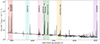 |
Fig. 1. Spectrum of an H II region (Galaxy: NGC 5068, region ID: 268) with the six spectral regions from Table 1 highlighted in different colours. Auroral lines are the faintest lines of the spectrum, with typical intensities ∼100 times less intense than nebular lines and ∼1000 times less intense than hydrogen recombination lines. |
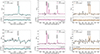 |
Fig. 2. Example fits (both stellar continuum and emission lines) of spectral regions around auroral lines for two H II regions in NGC 5068 (IDs: 268 in the upper panels, the same as Fig. 1, and 817 in the lower panels). The [NII]λ5756, [SIII]λ6312 and [OII]λλ7320, 7330 auroral lines are detected with corresponding S/N of 29, 39, 22, and 20 for region 268 and 6, 7, 7, and 7 for region 817. The flux in the y axis is expressed in the same units as Fig. 1. In the lower panels, we additionally report as a shaded region the spectral error band, already re-scaled by the residuals’ standard deviation. |
With respect to the fitting procedure adopted in Groves et al. (2023), the choice of fitting restricted wavelength intervals rather than the entire spectrum prevented us from tying the line kinematics over the total spectrum. We therefore imposed kinematic constraints within the individual spectral regions by fixing the velocity and velocity dispersion of weak lines to strong lines, if available; for example, the [S III]λ6312 auroral line to the [O I]λ6300 nebular line, or nitrogen and sulphur nebular lines to Hα. Details of the lines fitted in each wavelength intervals are presented in Table 1.
The most compelling check for evaluating the goodness of our procedure concerns the consistency of the different kinematic parameters calculated independently for each spectral region. Hence, we verified that both the velocity and the velocity dispersion evaluated independently for each spectral region are consistent, at least for the brightest emission lines (Hα, Hβ, [O III]λ5007).
2.1.2. Auroral line detections
The task of selecting reliable auroral line detections is particularly delicate due to their relative faintness and the fact that they can be easily confused with noise spikes. To identify reliable detections, we first required a threshold of 5 for each line in the amplitude-over-noise ratio (ANR), which we considered as a proxy of the S/N. We evaluated the amplitude as the line peak, while the noise was estimated as the standard deviation of the residuals between the data and the best fit around the line of interest. Requiring a simultaneous 5σ detection of [N II]λ5756, [S III]λ6312 and [O II]λλ7320, 7330 leads to a sample of 116 regions. For this sub-sample, the Hα and Hβ lines have S/N > 400, reaching values of several thousand for Hα; the [O III]λ5007 and [N II]λ6584 nebular lines are always detected with S/N > 130 and the [S III]λ9069 nebular line, which is slightly weaker than the other two, generally shows S/N > 40. For these bright regions, potential contributions from DIG can be safely neglected.
Secondly, we checked that the intrinsic width of the best-fit Gaussian for each auroral line does not significantly differ from the one for Hα. In particular, we required that |σ − σHα|≤0.4σHα. This condition allowed us to exclude any residual noise spikes and reduced our sample of regions with detections in all three auroral lines to 95, that is, 0.3% of the parent sample.
Finally, since the catalogue from Groves et al. (2023) includes gaseous regions of various nature, we used the Baldwin-Phillips-Terlevich (BPT) diagrams (Baldwin et al. 1981) to select H II regions. We verified that the 95 spectra that match our previous selection criteria are classified as H II regions in the [N II]/Hα versus [O III]/Hβ BPT diagram according to the demarcation line of Kauffmann et al. (2003), and are therefore all bona fide H II regions.
In Table 2, we summarise the statistics of auroral line detections in H II regions within our sample of galaxies. Reliable auroral lines detections (with S/N > 5 and with reliable kinematics parameters) are obtained only for a few percent (∼0.1% to ∼10%) of the nebulae in each galaxy. The [N II]λ5756 line is the most commonly detected line, with a total of 969 detections over 31497 regions (∼3% of the sample). Conversely, [S III]λ6312 is the most difficult line to detect, and our analysis provides only for 173 good line detections (0.55% of the total sample). Despite the fact that the mean spectral noise does not vary significantly along the available spectral coverage, such differences in auroral line detections arise because of the different continuum contamination due to telluric lines around auroral lines, which significantly affect the estimation of residuals’ standard deviation, and hence the line ANR. This effect is particularly evident for the [O II] auroral lines (right panels in Fig. 2), around which the standard deviation of residuals is typically a factor of two larger than around the [N II] auroral line (see also Fig. A.1). We observe that in Fig. 2 the spectral error is represented as a shaded region overplotted to the residuals between the flux and our model. In particular, the error is corrected by the normalisation factor, the standard deviation of residuals over median of the error vector, to take into account for the understimate in the spectral noise (Emsellem et al. 2022).
Total number of nebulae, along with the number of H II regions meeting the selection criterion individually for each auroral line and simultaneously for all lines, for each galaxy in the PHANGS-MUSE sample.
2.2. Ancillary datasets
We complemented the PHANGS–MUSE auroral lines dataset with high-quality, homogeneous catalogues of auroral line detections from the literature in order to compare with measurements of Te and chemical abundances over a wider metallicity range. Since the PHANGS–MUSE galaxies cover the metallicity range around solar (Groves et al. 2023), we specifically complemented them with the catalogue from Guseva et al. (2011) (G11 from now on) targeting low-metallicity objects, including also blue compact dwarf (BCD) galaxies. We also included the catalogues described in Nakajima et al. (2022) and Isobe et al. (2022) (denoted as N22 in the following), which target extremely metal-poor galaxies (EMPGs) from the EMPRESS (Extremely Metal-Poor Representatives Explored by the Subaru Survey) project. For comparison purposes, we considered the data from the CHAOS (CHemical Abundances Of Spirals) project. CHAOS encompasses observations of nearby, star-forming spiral galaxies carried out with the Multi-Object Double Spectrograph (MODS, Pogge et al. 2010) at the Large Binocular Telescope (LBT). In this work, we included the catalogues of H II regions from the six galaxies presented in Berg et al. (2020) and Rogers et al. (2021, 2022). Finally, we also compared our data with the line ratios obtained by Curti et al. (2017) (denoted as C17 in the following) by stacking Sloan Digital Sky Survey (SDSS) Data Release 7 (Abazajian et al. 2009), with galaxies stacked according to their values of reddening-corrected [O II]λλ3726, 3729/Hβ and [O III]λ5007/Hβ line ratios. In general, the line fluxes in C17 will include contributions from multiple H II regions, DIG, and other ionisation sources.
To obtain a homogeneous set of physical parameters, especially temperatures and ionic abundances, we re-analysed all the selected literature catalogues (although without re-fitting their spectra), trying to adhere to the same selection and data analysis procedures applied to the PHANGS–MUSE sample to the greatest extent possible. This implies using only the same emission lines available for the PHANGS–MUSE data, when possible. For this reason, we tried to avoid using the [O III]λ4363 auroral line present in all the other catalogues. The details of this analysis are presented in Appendix B. We also applied to all the catalogues the S/N threshold of 5 for line detections.
Additionally, we selected some of the most recent high-redshift publications reporting auroral line detection with NIRSpec (Near Infrared Spectrograph) on JWST, in particular from Sanders et al. (2023) and Laseter et al. (2024). Both summarise and further expand on the auroral line detections reported in the JWST Early Release Observations (ERO) programme (Pontoppidan et al. 2022; Arellano-Córdova et al. 2022; Schaerer et al. 2022; Curti et al. 2023). In particular, Sanders et al. (2023) report detections of the [O III]λ4363 auroral line for a sample of 16 galaxies at z = 1.4 − 8.7 from the Cosmic Evolution Early Release Science (CEERS) survey programme (Finkelstein et al. 2023a,b), while Laseter et al. (2024) presents [O III]λ4363 detections for 10 galaxies at z = 1.7 − 9.4 from the JWST Advanced Deep Extragalactic Survey (JADES) programme (Eisenstein et al. 2023). The procedure followed for determining oxygen abundances from these high-redshift data differs from that of the low-redshift catalogues because of the limited number of available emission lines, and is detailed in Appendix B.
3. Methods
3.1. Electron temperatures
The optimal approach to determine Te consists of simultaneously constraining both electron temperature and electron density using specific temperature- and density-dependent line ratios (but see Kreckel et al. 2022 for the introduction of an alternative approach). The temperature-sensitive line ratios available in the datasets considered in this work are summarised in Table 3. For density measurements, we consistently used the [S II]λ6731/[S II]λ6717 ratio.
Temperature-sensitive lines available for each catalogue.
For the PHANGS–MUSE data, and other catalogues that have not already been corrected for dust extinction, we have adopted the extinction law from O’Donnell (1994) with RV = 3.1 and an intrinsic Balmer ratio of Hα/Hβ = 2.86 to perform a reddening correction. For PHANGS–MUSE, we obtain AV values spanning the range from 0 to 1.3 mag, with a median of ∼0.7 mag.
With regard to density tracers, the [S II] line ratio is sensitive to density in the range of ne ∼ 102 − 104 cm−3. However, the majority of our selected H II regions are characterised by ne < 100 cm−3, that is, near or well below the low-density limit. For line ratios below the low-density limit, which was set at ne = 40 cm−3 following Kewley et al. (2019b), we imposed a fixed ne value of 20 cm−3. In this regime, varying the electron density does not significantly affect the final ionic abundance results.
In PHANGS–MUSE, we inferred Te from both the [N II]λ5756/[N II]λ6584 (Te[N II]) and the [S III]λ6312/[S III]λ9069 (Te[S III]) auroral-to-nebular line ratios. We calculated ne, Te[S III] and Te[N II] for the 95 selected PHANGS–MUSE H II regions using the PYNEB python package (Luridiana et al. 2012, 2015), version 1.1.15. Specifically, we used the GETTEMDEN function to infer the temperatures when ne was fixed at 20 cm−3 (54% of selected H II regions), and GETCROSSTEMDEN to get both ne and Te for regions outside the low-density limit. In our analysis, we do not find density values exceeding 200 cm−3.
We assumed Te[N II] to be representative of the whole low-ionisation zone, and used it to estimate the N+, S+, and O+ abundances, since MUSE does not allow a direct measurement of these electron temperatures. This assumption is supported by predictions from photoionisation models, although various studies (Rogers et al. 2021; Méndez-Delgado et al. 2023b; Rickards Vaught et al. 2024) show some discrepancies between Te estimates derived from the [N II], [O II] and [S II] temperature-dependent line ratios. Finally, we used Te[S III] to determine the S2+ abundance within the intermediate-ionisation zone.
We exploited the two temperature measurements in the PHANGS–MUSE data to re-calibrate the Te[S III]–Te[N II] relation. Using a Monte Carlo Markov Chain (MCMC) approach, we obtained the following best-fit relation:
![$$ \begin{aligned} T_{\rm e} [\mathrm{S}\,{\small {\text{III}}} ] = 1.22 ({\pm }0.01)\, T_{\rm e} [N\,{\small {\text{II}}} ] - 0.20({\pm }0.01) , \end{aligned} $$](/articles/aa/full_html/2024/11/aa51007-24/aa51007-24-eq1.gif)
with temperatures expressed in units of 104 K. This relation (Fig. 3) is consistent within 1σ with previous calibrations based on analyses of H II regions in nearby galaxies, encompassing also the CHAOS sample (Croxall et al. 2016; Rogers et al. 2021) and a restricted sub-sample of seven galaxies within the PHANGS-MUSE dataset (Rickards Vaught et al. 2024). The consistency with the latter calibration is significant as it represents a completely independent analysis of auroral lines in PHANGS-MUSE HII regions. Nevertheless, the correspondence between the two calibrations is not perfect, as there is a clear offset. The major difference between our work and the one of Rickards Vaught et al. (2024) lies in the identification of H II region borders and subsequent extraction of line fluxes, with their apertures being typically larger than ours because of the larger PSF of the Keck Cosmic Web Imager (KCWI) instrument relative to MUSE (see their Sect. 2 for more details). The different morphology of H II regions will have a greater impact on low-ionisation ions found towards the outer regions of ionised nebulae, whereas ions in the intermediate- and high-ionisation zones are expected to be less influenced by differences in H II region boundaries. We tested this hypothesis by cross-matching in co-ordinates the H II regions from Rickards Vaught et al. (2024) and the ones defined as in Groves et al. (2023) and used in this work. We obtained 32 matches, for which we compared the Te[S III] and Te[N II] estimates. We found that the two Te[S III] estimates are in good agreement, while the Te[N II] values derived in Rickards Vaught et al. (2024) show a median bias of −570 K with respect to ours. This result explains the offset between the two Te[S III]–Te[N II] calibrations observed in Fig. 3, and allows us to conclude that the main difference in the two works is due to the different setting of H II region borders.
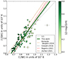 |
Fig. 3. Resulting MCMC best fit (in dark green) of the Te[N II]–Te[S III] relation calibrated on PHANGS-MUSE data, which are reported and colour-coded according to their metallicity value (see Sect. 3.2). Other calibrations from previous literature works are reported for comparison; the five curves show comparable behaviours. |
We estimated the intrinsic dispersion σint about the best-fit Te[S III]–Te[N II] relation following the same approach outlined in Rogers et al. (2021). We fixed the slope and intercept of the relation to the best-fit parameters of the linear fit; then we sampled the parameter space using an MCMC to determine the σint value that maximises the likelihood function. We find σint = 724 ± 55 K, which is higher than the corresponding values found in Rogers et al. (2021) (σint = 173 K), but lower than the one found in Rickards Vaught et al. (2024) (σint = 997 K). In general, σint is significantly higher than the typical errors associated with our PHANGS–MUSE Te[S III] error measurements, which have a median value of ∼70 K.
We carried out a similar procedure (Appendix B) to evaluate ne and Te for the literature catalogues. We used these to re-calibrate the Te[O III]–Te[S III] relation using temperature measurements from the CHAOS and G11 catalogues, the only datasets in our compilation where Te[O III] and Te[S III] are directly measured (Fig. B.2). We find a Te[O III]–Te[S III] relation consistent with previous works.
We used the Te[O III]–Te[S III] relation for estimating the temperature associated with the high-ionisation zone (traced by the O2+ ion) in PHANGS–MUSE data, where we do not have access to [O III]λ4363. In principle, we could have alternatively re-calibrated the Te[O III]–Te[N II] relation to infer Te[O III], but Rogers et al. (2021) reported that the Te[O III]–Te[S III] relation shows a tighter correlation than the Te[O III]–Te[N II] relation.
3.2. Ionic abundances determination
Once the electron temperatures and densities were measured, we could estimate ionic abundances through the ratio of a collisionally excited emission line to a Balmer recombination line, usually Hβ (Garnett 1992; Pérez-Montero 2017). All the ionic abundances discussed in this section were evaluated with PYNEB, using the GETIONABUNDANCE function. In particular, we adopted the PYNEB default atomic data and the dust-corrected Hβ as the reference hydrogen recombination line.
Errors on ionic abundances (and on electron temperatures and densities) were computed with Monte Carlo simulations: for each of the 95 selected H II regions from the PHANGS–MUSE sample, we generated 500 realisations of emission line fluxes of interest, according to a Gaussian distribution centred on the measured flux and with σ equal to the measured error. For each realisation, we carried out dust correction, evaluated line ratios, and measured Te, ne, and ionic abundances. We took the median and the standard deviation of the resulting parameter distributions as the best value and corresponding error to associate with each parameter, respectively.
When possible, ionic abundance measurements were carried out exploiting nebular lines rather than auroral lines, because they are brighter and detected at higher S/N. As is summarised in Table 4, this is the case for N+, S+, S2+, and O2+. However, the ionic abundance of O+ was measured with the [O II]λλ7320, 7330 auroral lines, as the [O II]λλ3726, 3729 nebular lines are not covered by MUSE. The [O II] auroral lines could be contaminated due to recombination (Rubin 1986; Pérez-Montero 2017), so to demonstrate the validity of this approach we compared the O+ ionic abundance evaluated from auroral and nebular lines for those catalogues for which the two sets of lines are both available (CHAOS, C17 and G11 catalogues). This comparison (see Fig. B.1) shows a consistency between the two measurements, validating our approach.
Temperature estimates and collisionally excited line fluxes used for measuring ionic abundances.
We computed the oxygen abundance as the sum of the two ionic species, O+ and O2+:
neglecting potential contributions from O3+, which is typically minimal in H II regions (Draine 2011).
Figure 4 reports the O+ (upper panel) and O2+ (middle panel) abundances and the O2+/O+ fraction (lower panel) as a function of the total oxygen abundance, with PHANGS–MUSE data points colour-coded according to their Te[N II] value. From the first panel of Fig. 4, we observe that H II regions with lower temperatures are characterised by higher metallicities and higher O+/H+ values, with O2+ representing only a small contribution of 20 − 30% when 12 + log(O/H)≳8.4. Unlike the top panel, no evident trends are observable for O2+ abundance (middle panel of Fig. 4), although the O2+/O+ fraction appears to decrease when the total oxygen abundance increases (bottom panel of Fig. 4). Similar trends were also presented by C17.
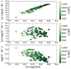 |
Fig. 4. O+ abundance (upper panel), O2+ abundance (middle panel), and relative ionic abundance of the two species (bottom panel) as a function of the total oxygen abundance for the 95 selected H II regions from the PHANGS-MUSE nebular catalogue. |
While the two most abundant ionic species of oxygen exhibit bright emission lines in the optical, most other elements lack bright lines from all of predominant ionic states within the same wavelength range. Therefore, determining their total abundances requires an ionisation correction. In particular, under typical H II region physical conditions nitrogen is found mostly in the form of N+ and N2+, and sulphur in the form of S+, S2+ and possibly S3+, but the N2+ and S3+ ions do not present emission lines in the spectral range covered by MUSE. To calculate the total abundance of these elements, we introduced an ionisation correction factor (ICF):

where for simplicity we have introduced the notation X = N(X)/N(H).
Various sulphur and nitrogen ICF parametrisations exist in the literature, generally expressed as a function of O+/O. In Stasińska (1978), a first example of sulphur ICF was provided, which was subsequently updated in Pérez-Montero et al. (2006), Kennicutt et al. (2003), and Dors et al. (2016). Peimbert & Costero (1969) reported the first expression for the nitrogen ICF, subsequently adopted in Thuan et al. (1995) and in the works from the CHAOS team. Izotov et al. (2006) proposed new expressions for both the sulphur and the nitrogen ICFs as a function of O+/O and further introduced a dependence on the system metallicity or, analogously, on its electron temperature.
For the sulphur and nitrogen abundances, we adopted the following parametrisations from Izotov et al. (2006):


where the low-metallicity regime is defined as 12 + log(O/H)≤7.6 and the high-metallicity regime as 12 + log(O/H)≥8.2, and v = O+/O parameter. We found that the majority of H II regions from the PHANGS–MUSE sample do not require corrections for sulphur ICF. In most cases, the ionisation correction is negligible compared to typical errors on ionic abundances, and applying it would only increase their uncertainty. The sulphur ICF is significant only in 8 of 95 H II regions. Even in these cases, the correction remains minimal, reaching a maximum value of 1.06 that corresponds to a relative variation in the sulphur abundance of only ∼6%. In contrast, nitrogen ICF has a more significant effect on all the H II regions of the sample, especially the ones at lower metallicity. ICF(N+) is characterised by minimum, median and maximum values of 1.06, 1.33, and 2.45, respectively, which correspond to relative variations in nitrogen abundance of 5%, 25% and 60%. The maximum ICF(N+) value of 2.45 is found for the only PHANGS-MUSE H II region with metallicity < 8.1.
Trends between oxygen and sulphur and nitrogen abundances are reported in Fig. 5 for both the PHANGS-MUSE sample and the other literature samples described in Sect. 2.2. The upper panels show that both sulphur and nitrogen abundances increase with oxygen abundance. The lower panels report instead the logarithmic S/O and N/O ratios, again as a function of the system metallicity, so that the relative abundance of sulphur and nitrogen with respect to oxygen can be quantified. We see a net decreasing trend of log(S/O) with log(O/H), while log(N/O) appears to be almost constant, despite a significant scatter. More quantitatively, we carried out a linear fit of log(S/O) and log(N/O) as a function of log(O/H) and found:
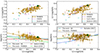 |
Fig. 5. Upper panels: Sulphur and nitrogen chemical abundances versus total system metallicity for the PHANGS–MUSE sample and the other analysed literature catalogues. Lower panels: Relative abundances of sulphur and nitrogen with respect to oxygen, as a function of the total system metallicity. Solar values from Asplund et al. (2009) are reported as teal points for comparison. We display linear trends calibrated either using only the PHANGS-MUSE data or the entire dataset, which also includes literature data. The other log(S/O) versus 12 + log(O/H) trends are from Izotov et al. (2006) and Dors et al. (2016), with the former calibrated over BCD galaxies and the latter over a compilation of literature emission-line intensities of H II regions and star-forming galaxies and while considering sulphur ICF from Thuan et al. (1995). The log(N/O) versus 12 + log(O/H) trend is taken from Nicholls et al. (2017) and it is calibrated over a compilation of literature stellar data. |


when considering only PHANGS-MUSE data, and:


when considering the available literature catalogues too.
A decreasing trend for log(S/O) versus O/H, similar to the one presented in Fig. 5, has previously been reported in the literature (Pérez-Montero et al. 2006; Dors et al. 2016; Díaz & Zamora 2022). In Pérez-Montero et al. (2006), the decreasing trend in log(S/O) appears evident in particular for H II galaxies and giant extragalactic H II regions (their Fig. 5). Instead, in Dors et al. (2016) and Díaz & Zamora (2022) a sample of star-forming galaxies and H II regions was analysed, and they both found a log(S/O) versus log(O/H) trend similar to ours, both in shape and normalisation, although Dors et al. (2016) measurements show a slight offset towards lower log(S/O). However, other works in the literature (Izotov et al. 2006; Maciel et al. 2017) found a roughly constant trend of S/O with metallicity. Since both sulphur and oxygen are α elements primarily produced through type II supernovae, this flat trend is generally expected. The variation observed here and in other works could indicate a metallicity dependence in the production of α elements by these massive stars, as suggested in Guseva et al. (2011). This hypothesis finds further confirmation in the fact that such a trend is particularly evident for single H II regions rather than whole galaxies, suggesting a strict connection with local stellar nucleosynthesis and chemical evolution processes.
Moving now our focus onto nitrogen, we observe that, despite the large scatter, a similar range of values is found in Gusev et al. (2012) or Pérez-Montero & Contini (2009), while other works, such as Castellanos et al. (2002) and Pilyugin et al. (2003, 2010), found an increasing trend of log(N/O) with log(O/H) at high metallicities and a flat behaviour in the low-metallicity regime, with the turning point roughly located at metallicities of ∼8.4. The independence of log(N/O) on metallicity in the low-metallicity regime suggests that nitrogen is a primary element, that is, its production does not depend on the presence of other heavy elements. However, this metallicity regime is not covered by our PHANGS–MUSE data. The increasing trend found in some literature works at higher metallicity may be due to a secondary, metallicity-dependent production of nitrogen, as was first proposed in Vila-Costas & Edmunds (1993) and then adopted, for example, in Nicholls et al. (2017). The reason for the large scatter observed in our data cannot be readily identified.
3.3. Ionisation parameter measurements
The ionisation parameter is typically inferred by comparing two emission lines from the same atomic species originating from different ionisation states, with the most sensitive diagnostics coming from two states with the largest difference in ionisation potentials. The line ratios most commonly used to trace the ionisation parameter in the optical wavelength range are [S III]λλ9069, 9531/[S II]λλ6717, 6731 and [O III]λ5007/[O II]λλ3726, 3729. In the PHANGS–MUSE spectral range we estimate the flux of the [S III]λ9531 from the observed [S III]λ9069 flux, assuming a fixed ratio of 2.469. With this arrangement, the sulphur line ratio can be evaluated for PHANGS-MUSE, CHAOS and G11 catalogues, while the oxygen line ratio is available for CHAOS, C17, G11 and N22 catalogues, as well as for high-redshift data from Sanders et al. (2023) and Laseter et al. (2024).
There are various existing literature calibrations for determining the ionisation parameter, based on comparisons between diagnostic line ratios and photoionisation models. We test log(U) calibrations from Morisset et al. (2016), Kewley & Dopita (2002) and Kewley et al. (2019b), using both oxygen and sulphur line ratios according to the line availability in the various catalogues. We find significant discrepancies in log(U) estimates obtained with different literature calibrations for the same line ratio, mostly in terms of a normalisation offset. Additionally, we also notice inconsistencies between ionisation parameter estimates obtained with calibrations from the same publication, but based on different line ratios when both sulphur and oxygen ratios were measured.
Among the calibrations considered, we adopted as fiducial the one from Kewley et al. (2019b), because their prescription produces the smallest discrepancies in the log(U) estimates from the oxygen and sulphur lines. The measured log(U) values for the 95 regions in PHANGS–MUSE with auroral line detections are shown in Fig. 6. In general, the log(U) values for the selected PHANGS-MUSE H II regions are slightly lower than the ones reported in literature (where typically log(U) spans from −3.6 to −2.6, see e.g. Poetrodjojo et al. 2018; Grasha et al. 2022), with a peak around log(U)∼ − 3.5. This discrepancy may partially be due to the fact that PHANGS–MUSE H II regions are characterised by higher metallicities with respect to the majority of analysed H II regions in the literature, or it may be a consequence of using sulphur line ratio for inferring log(U), since the [S III]/[S II] line ratio tends to underestimate the ionisation parameter with respect to the oxygen line ratio (Kewley & Dopita 2002).
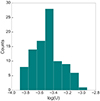 |
Fig. 6. Measurements of ionisation parameter, log(U), for our sample of 95 H II regions. |
4. Results
4.1. Empirical calibration of strong-line diagnostics
In this section we present the calibration of strong-line diagnostics using a total sample of 168 direct metallicity measurements: 95 from PHANGS–MUSE, 24 from CHAOS, 27 from C17, 10 from G11 and 12 from N22 catalogues. The 95 HII regions from PHANGS–MUSE sample provide numerous data points extending into the solar metallicity regime. The combination of these data allows for the calibration of diagnostics simultaneously valid over a wide range of metallicities (7.4 ≤ 12 + log(O/H)≤8.82) and for different astrophysical sources, since our dataset is composed of both single H II regions and whole galaxies.
We calibrate R3 = [O III]λ5007/Hβ, N2 = [N II] λ6584/Hα, O3N2 = R3/N2 and N2S2Hα = N2/S2 ⋅ N20.264 (first proposed in Dopita et al. 2016 in its logarithmic form, with N2 = [N II] λ6584/Hα and S2 = [S II]λλ6717, 6731/Hα) diagnostics as a function of metallicity, as is shown in Figs. 7a, 7b, 7c, and 7d, respectively. Because of the absence of [O II]3726, 3729 nebular lines in PHANGS–MUSE spectra, we did not consider the popular R2 = [OII]3726, 3729/Hβ diagnostic and all the others derived from it, such as O32 = R3/R2 or R23 = R2 + R3.
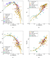 |
Fig. 7. Calibration of R3 = [O III] λ5007/Hβ (panel a), N2 = [N II] λ6584/Hα (panel b), O3N2 = R3/N2 (panel c), and N2S2Hα = N2/S2 ⋅ N20.264 (panel d) diagnostics carried out in this work (solid golden curves). Data points are colour-coded according to the original source catalogues, with golden points associated with PHANGS–MUSE data. The other curves report calibration from the literature for comparison. The dashed extension at low-metallicity shows the extrapolation of our calibrations. |
We fit each of the considered diagnostics using polynomials of the form:
where we test N = 2, 3, 4, R is the diagnostic, and x is the oxygen abundance normalised to the solar value from Asplund et al. (2009): x = 12 + log(O/H)–8.69. We fit these relations using the ODR python package, which performs orthogonal distance regression, taking into account the errors on both independent and dependent variables. We then select the polynomial that better fits our data by selecting the fit with the minimum value of χ2; in addition, we also applied the Bayesian information criterion (BIC) to confirm the model selection and a binning procedure that aims to give the proper weight to the few available low-metallicity data points. When these metrics are similar, we selected preferentially lower order polynomials. With the binning procedure, we divide the 12 + log(O/H) range into 10 bins of equal width, and for each bin we evaluate the median and standard deviation of line ratios and oxygen abundances. These binned values are then exploited to check manually the consistency of the different polynomial fits with the data points over the whole metallicity range. In particular, they allow for a better visualisation of the general trends both in the high-metallicity regime, where there are numerous single data points but characterised by significant scatter, and in the low-metallicity regime, where there are few but fundamental data points. We do not repeat the polynomial fitting procedure on the binned values, but we use them for visual confirmation of the best polynomial order to use while carrying out the fit over the whole sample of single data points.
Our best-fitting cn coefficients associated with the polynomial functional form from Eq. (14) are reported in Table 5 and the newly calibrated diagnostics are displayed as golden curves in Fig. 7. We also show calibrations from the literature for comparison. We consider the validity regime of our calibrations to cover the range 12 + log(O/H) = [7.4−8.9], given the increasingly small number of datapoints at lower and higher metallicities.
cn coefficients for our strong-line diagnostic calibrations.
Specifically, R3 is fitted using a N = 3 polynomial to take into account the well-known double branch behaviour. In general, there is a good agreement between our R3 calibration and the ones from Curti et al. (2017) and Nakajima et al. (2022), although our result suggests a steeper decrease at 12 + log(O/H) ≳ 8.5. At these metallicities most of the data come from our new PHANGS–MUSE detections. Additionally, the high-redshift data reported in this plot (blue and pink dots, taken respectively from Laseter et al. 2024; Sanders et al. 2023) show slightly elevated R3 with respect to local data in the same metallicity regime. The pink curve, which provides an excellent fit to these data, is one of the first high-redshift diagnostic calibrations, presented in Sanders et al. (2023) and valid over a redshift range spanning from Cosmic Noon to the Epoch of Reionisation and over the metallicity range 12 + log(O/H) = [7.0–8.3].
We fit the N2 diagnostic using a N = 4 polynomial, in agreement with previous literature calibrations, while O3N2 is fitted using a N = 3 polynomial, differing from both Curti et al. (2017) and Nakajima et al. (2022) where a N = 2 polynomial is adopted. The difference in the choice of the polynomial order for O3N2 is only evident in the low-metallicity regime, which is still poorly populated. Lastly, the N2S2Hα diagnostic is fitted using a N = 2 polynomial, and our calibration is consistent with the linear trend found in Dopita et al. (2016) for its logarithmic form. Despite the fact that our sample encompasses only data points from Nakajima et al. (2022) at 12 + log(O/H) ≤ 8.0, our diagnostic calibrations differ from those reported in the same work; this is due to the different high-metallicity samples adopted in the two analysis. In fact, Nakajima et al. (2022) integrate their low-metallicity sample of EMPGs with data from Curti et al. (2017), while we also consider the CHAOS sample and especially the PHANGS-MUSE data points. This translates into significantly different final samples, with our dataset more biased towards the high-metallicity regime.
Apart from these four diagnostics, we additionally calibrated S2, N2S2 = N2/S2, RS23 = R3 + S2 and O3S2 = R3/S2, but we did not include them in our analysis for the following reasons: (1) they are characterised by significantly larger scatter with respect to the four diagnostics reported in Fig. 7; (2) for those diagnostics where a calibration was carried out, we compared the indirect metallicity estimates obtained by combining only R3, N2, O3N2 and N2S2Hα diagnostics with the results obtained by further adding O3S2, RS23 and N2S2 in all the possible combinations, and we found no significant difference in the final values. Thus we conclude that these diagnostics do not contribute to an improvement of indirect estimates of metallicities, but only add uncertainties due to their larger scatter. We therefore do not consider them further.
To validate our analysis, we compared the direct metallicity measurements, as carried out in Sect. 3.2, with the corresponding indirect estimates obtained by minimising the chi-square defined simultaneously by all the selected diagnostics (R3, N2, O3N2 and N2S2Hα) as:
where the sum is carried out over the different diagnostics, Robs, i are the observed line ratios, σobs, i are the associated uncertainties, and Rcal, i are the values predicted by each calibration for a given metallicity. In principle, one could also consider the intrinsic dispersion of each strong-line diagnostic calibration (the RMS column in Table 5), in order to attribute a major weight to the diagnostics with lower intrinsic scatter. However, because such scatter is comparable for all the diagnostics and always dominant by one or two orders of magnitude with respect to the observed line ratio uncertainties, we find that considering the intrinsic scatter does not change the final χ2 minimisation procedure.
This comparison is reported in Fig. 8. In general, there is a good agreement between direct and indirect metallicity estimates over the whole metallicity range, although at high metallicity (12 + log(O/H) ≳ 8.0) the scatter around the 1:1 relation becomes significant (RMS of residuals: 0.14 dex). If we consider only PHANGS–MUSE data (dark green points), there exists a trend of residuals with metallicity, with indirect measurements overestimating the corresponding Te-based metallicity at 12 + log(O/H) ≲ 8.5 and underestimating them at higher metallicities. These data points at 12 + log(O/H) ≲ 8.5 that significantly deviate from the 1:1 relation are the same that significantly deviate from the best fit relations in Fig. 7. As such deviations are already evident in the calibration plots, we conclude they are not due to potential inaccuracies in our calibrations but to limitations in the direct measurements themselves, the primary ones being the simplification in the assumed three-zone theoretical model and the hypothesis of an homogeneous ISM. To a lesser extent, some effects may arise from selection biases since working with auroral lines limits the study to the brightest H II regions. Nonetheless, we verify that increasing the ANR threshold to 7 or 10, instead of 5, still yields consistent results without reducing the scatter in the data points. We conclude that, because strong-line ratios are influenced by many factors beyond the source metallicity – such as the physical and geometrical structures of ionised nebulae –, their calibration remains complex and highly dependent on the specific sources. Addressing this requires abandoning the current simplifications and conducting a comprehensive analysis of these regions, extending beyond the narrow focus on the single chemical aspect.
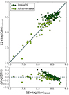 |
Fig. 8. Comparison between direct metallicity estimates (x axis) and indirect metallicity estimates (y axis) obtained using the calibration based on R3, N2, O3N2 and N2S2Hα diagnostics proposed in this work. Data points are divided into PHANGS–MUSE data (dark green points) and all the other data taken from the literature catalogues (light green points). The solid line is the 1:1 relation. |
Inspired by the recent work from Easeman et al. (2024), we also compared our direct metallicity measurements with the indirect ones obtained using only the N2S2Hα diagnostic, which Easeman et al. (2024) consider the most reliable strong-line diagnostic when working with MUSE data. However, we did not find significant differences in indirect estimates by using only the N2S2Hα diagnostic or by combining it with R3, N2 and O3N2. We therefore prefer to use in our fiducial calibration the combination of all four line ratios we have calibrated. This could also help minimise spurious effects arising from the use of a single strong line diagnostic due to secondary dependencies on sulphur and nitrogen abundances (Dopita et al. 2016; Maiolino & Mannucci 2019).
4.2. Dependence of strong-line diagnostics on ionisation parameter
In this section we test whether the scatter observed in the strong-line calibration plots of Fig. 7 can be attributed to the degeneracy between metallicity and ionisation parameter, as these two parameters are known to be strongly anti-correlated (Morisset et al. 2016; Ji & Yan 2022). We study the dependence of strong-line diagnostics on log(U) by both evaluating the ionisation parameter for our dataset in terms of sulphur and oxygen line ratios, as was discussed in the previous section, and by analysing photoionisation models.
In Fig. 9 we report the same diagnostics as in Fig. 7, but with data points colour-coded according to the sulphur and oxygen line ratios used as a proxy for the ionisation parameter. We can identify some clear trends in these plots, particularly evident for the [O III]/[O II] line ratio, with data points at lower metallicities characterised by higher [O III]/[O II] and [S III]/[S II] line ratios, which correspond to higher ionisation parameter values. On the other hand, at higher metallicities the situation becomes more complex and the scatter is significant. The same line ratio value on the y axis can be associated with different metallicity values because of the degeneracy of metallicity with log(U), implying that the scatter observed in these plots encodes the further dependence of strong-line ratios on other physical properties apart from the metallicity of the source. To further investigate this additional dependence, we turn to photoionisation models.
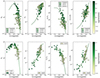 |
Fig. 9. Dependence of strong-line diagnostics on the ionization parameter. Upper panels: Strong-line diagnostics colour-coded according to the [S III]λλ9069, 9531/[S II]λλ6717, 6731 line ratio. Lower panels: Strong-line diagnostics colour-coded according to the [O III]λ5007/[O II]λλ3726, 3729 line ratio. We have labelled as ‘local’ the data from CHAOS, Curti’s, Guseva’s and Nakajima’s catalogues and as ‘high-z’ data from Sanders et al. (2023) and Laseter et al. (2024). The plotted curves are our diagnostic calibrations plus the high-redshift calibration from Sanders et al. (2023) for R3. |
We consider Cloudy photoionisation models3 described in Belfiore et al. (2022). They used input spectra generated with the Flexible Stellar Population Synthesis (FSPS) code (Conroy et al. 2009), using simple stellar population (SSP) models (Byler et al. 2019), with ages between 0.5 Myr and 20 Myr, spanning a metallicity range of [Z/H] = [−0.6, 0.4], and an ionisation parameter range of log(U) = [−5, −1] (local H II regions showing typical log(U) values of [−3.6, −2.6], see e.g. Grasha et al. 2022; Poetrodjojo et al. 2018). The corresponding input gas-phase metallicities vary in the range 12 + log(O/H) = [6.5, 9.0]. As we are interested in studying star-forming regions, we focus on young SSP spectra with age of 0.5 Myr, although very similar results are obtained by considering ages up to ∼5 Myr. The median age of PHANGS-MUSE stellar clusters associated with H II regions is ∼4 Myr (Scheuermann et al. 2023). We applied the same data analysis procedure to the models as to the observational data. In particular, we estimated Te and ionic abundances for each model following the same procedure as in Sect. 3. In Fig. 10, we show the resulting line ratios as a function of our estimate of the strong-line metallicity applying the calibration developed in this work to the models.
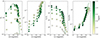 |
Fig. 10. Dependence of strong-line ratios on log(U) resulting from the photoionisation model analysis carried out in this work. To realise this figure, in particular, we have analysed a 0.5 Myr SSP input spectrum. Data points are colour-coded according to their log(U) values. |
We observe that differences in ionisation parameter can account for the scatter present in strong-line diagnostics, especially R3 and O3N2, which show the largest dependence on log(U) (Maiolino & Mannucci 2019). We observe that the metallicity estimates reported on the x axis are the output metallicities, that is, the ones obtained by applying the direct method to the input line ratios. We compared these metallicity values with the input ones and found a general consistency that breaks only at high metallicities (12 + log(O/H) ≳ 8.5), with this effect more evident for higher ionisation parameters. This discrepancy, according to which photoionisation models systematically overestimate metallicity estimates with respect to empirical methods, is well known in literature (Marconi et al. 2024 and references therein).
5. Effect on metallicity gradients
In this section we consider the effect of our revised calibration on the measurements of metallicity gradients. Specifically, we compare with the metallicity gradients measured for the PHANGS–MUSE sample by Groves et al. (2023). For each galaxy in the PHANGS–MUSE sample, we select all the nebulae from the catalogue of Groves et al. (2023) with S/N > 5 on the lines that define the R3, N2, O3N2 and N2S2Hα diagnostics, namely: Hα, Hβ, [O III]λ5007 [N II]λ6584, [S II]λλ6717, 6731, [S III]λ9069. We select H II regions by applying the same BPT diagram selection mentioned in Sect. 2.1.2. These cuts result in the selection of 23704 H II regions out of 31497 initial entries. We then use Eq. (15) to indirectly estimate metallicity according to our calibration.
In Fig. 11 we report the 2D distribution of H II regions metallicities for four of the 19 galaxies of the PHANGS–MUSE sample, to illustrate the variety of distributions. Each H II region is colour-coded according to its strong-line metallicity estimate, apart from those with a direct measurement available, which are shown as large diamonds.
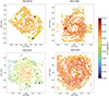 |
Fig. 11. 2D metallicity distribution of H II regions in NGC 0628, NGC 1566, NGC 2835 and NGC 4303. H II regions in each galaxy are colour-coded according to their metallicity. Indirect estimates are shown with dots, direct measurements with diamonds. |
We fit linear slopes to the metallicity gradient in units of effective radius (Reff). The best fits are reported in Table 6 for each galaxy. We fit two different radial gradients for each galaxy: one that considers all H II regions and one that excludes those within r < 0.5 Reff, as was first proposed in Sánchez-Menguiano et al. (2018) and then adopted in Groves et al. (2023). For each galaxy, we also evaluate the standard deviation of the metallicity residuals with respect to the best-fit linear gradient, σ(O/H), which we report in the last column of Table 6. We find that σ(O/H) varies from 0.022 to 0.039 dex, with a mean value across the sample of σ(O/H) of 0.031 dex.
Radial metallicity gradients for the 19 galaxies in the PHANGS–MUSE sample.
We compare the metallicity gradients obtained by using our strong-line diagnostics for indirect metallicity estimates with the same gradients based on the literature calibrations from C17, N22, and Pilyugin & Grebel (2016), abbreviated as PG16 in the following. In Fig. 12 we show a comparison of indirect metallicity estimates based on our, C17, N22 and PG16 calibrations for the whole PHANGS–MUSE H II region sample. In general, the PG16 calibration provides lower metallicities with respect to those estimated in this work, or from the calibrations of C17 and N22 (left panel of Fig. 12), with this discrepancy more evident at lower metallicities (12 + log(O/H) ≲8.3). Conversely, the C17 and N22 calibrations provide slightly higher metallicity values with respect to our calibration (central and right panels of Fig. 12). Despite the clear presence of an offset between the two calibrations, they present a 1:1 relation that breaks only at high metallicities (12 + log(O/H) ≳ 8.7).
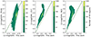 |
Fig. 12. Comparison between indirect metallicity estimates based on our calibration and on PG16, C17 and N22 calibrations (respectively: left, central, and right panels) for all H II regions in the PHANGS–MUSE sample. For each figure, the colourbar describes the contour lines of the metallicity distribution. The solid line indicates the 1:1 relation. |
To understand the origin of the discrepancy between the PG16 and our calibration, we tested the dependence of residuals on a number of secondary parameters: ionisation parameter (from the sulfur line ratio, estimated as in Sect. 3.3), χ2 (as defined in Eq. 15), and Hα flux, velocity dispersion, and equivalent width. We found no dependence on Hα flux, velocity dispersion, and equivalent width or χ2, and only a mild inverse correlation with ionisation parameter (Pearson correlation coefficient: 0.3).
We compare the metallicity gradients derived from different calibrations in Fig. 13 for four galaxies of the PHANGS–MUSE sample. The N22 calibration shows gradients characterised by significant, probably unphysical, scatter. The scatter is slightly reduced with C17 calibrations, and the lowest scatter is obtained when using the calibrations from this work or PG16 calibrations. In a few cases (one to three H II regions per galaxy) the PG16 calibration provides unphysically low metallicity estimates (typically 12 + log(O/H) ≲ 7.5), which are not shown in Fig. 13.
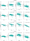 |
Fig. 13. Radial metallicity gradients for galaxies NGC 0628, NGC 1566, NGC 2835, and NGC 4303. Metallicity estimates are obtained with our, C17, N22 and PG16 calibrations (from left to right) and reported as small dots in each panel. Big diamonds are the direct measurements, not used to calibrate gradients but reported for visualisation purposes. The solid lines represent the linear best fit performed by excluding data at r < 0.5 reff, and small black dots are the indirect metallicity median values evaluated in 0.36 reff, 0.81 reff, 0.46 reff, and 0.62 reff wide bins, respectively. |
In Fig. 14 we provide a further comparison between the gradient slopes obtained when using the different calibrations for metallicity estimates. We first verify that the slopes obtained when using PG16 calibration are consistent with the ones provided in Groves et al. (2023), where the same calibration is adopted. Hence, in the upper panel of Fig. 14 we directly compare the slopes presented in Groves et al. (2023) with the ones based on the strong-line diagnostic calibrations presented in this paper. We observe that PG16 calibration provides systematically steeper gradient slopes with respect to ours, with this effect being stronger as the slopes become more negative. On the other hand, there is a substantially better agreement between our results and the ones obtained with N22 and especially C17 calibrations (in the lower and central panels of Fig. 14, respectively). From Fig. 12, we observe that our diagnostics tend to overestimate PHANGS–MUSE H II region metallicities at 12 + log(O/H) ≲ 8.4, suggesting a shrinking in the metallicity coverage relative to the direct method. This effect can lead to a slight underestimate in gradient slopes, and may be partially responsible for the discrepancies observed in Figs. 13 and 14 when comparing our results with the literature, especially PG16. Nevertheless, our results from Table 6 are consistent with the general trends of metallicity gradients observed in local star-forming galaxies, as reported in other studies. In Belfiore et al. (2017), for example, typical metallicity gradients for the SDSS IV Mapping Nearby Galaxies at Apache Point Observatory (MaNGA; Bundy et al. 2015) survey span from 0.0 to −0.1 dex/(r/Reff) for z ∼ 0 galaxies with masses log(M/M⊙) = 9.0 − 11.5, encompassing the mass range covered by the PHANGS–MUSE galaxies (Leroy et al. 2021). The CHAOS collaboration finds metallicity slopes around −0.1 dex/(r/Reff) (Rogers et al. 2021, 2022). Similar results are also reported in Sánchez et al. (2014) for the Calar Alto Legacy Integral Field Area (CALIFA) Survey (Sánchez et al. 2012), where gradient slopes are found to vary from −0.2 to 0.0 dex/(r/Reff) with a well-defined characteristic value of −0.1 dex/(r/Reff) and standard deviation of 0.09 dex/(r/Reff).
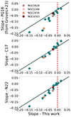 |
Fig. 14. Comparison between the slopes of metallicity radial gradients fitted on different metallicity estimates based on our PG16 (upper panel), C17 (middle panel), and N22 (lower panel) calibrations. The solid line is the 1:1 relation. For visual clarity, we have highlighted with different colours the four galaxies from Fig. 11. |
6. Conclusions
In this work, we provide a chemical analysis of H II regions from the PHANGS-MUSE nebular catalogue compiled in Groves et al. (2023). We fitted all the spectra from the catalogue following an innovative procedure based on single-region spectral fitting, with the intent of better constraining the stellar continuum. We carried out a selection procedure that aimed to select without any prior bias the brightest sources of the catalogue, then we exploited the measured line fluxes to estimate the electron temperatures and densities, and hence the ionic abundances. We complemented the PHANGS-MUSE emission line catalogue with other emission line compilations from the literature, which have been carefully re-analysed in order to obtain a homogeneous and comprehensive sample of direct metallicity estimates covering a wide range in metallicity (7.4 ≤ 12 + log(O/H)≤8.8). We then exploited the total dataset to empirically re-calibrate some of the most widely used strong-line diagnostics for the determination of the oxygen abundance, and we investigated their dependence on the ionisation parameter. Lastly, we used our newly calibrated diagnostics to infer the metallicity of all H II regions within the PHANGS-MUSE sample, and for each galaxy of the sample we evaluated the radial metallicity gradients. We summarise our main results as follows.
-
PHANGS-MUSE galaxies are characterised by significantly high gas-phase metallicities, with 12 + log(O/H) ≥ 8.0. Oxygen is found mostly in its singly ionised state (Fig. 4). Sulphur and nitrogen abundances are typically sub-solar (Fig. 5). The S/O ratio drops significantly as the source metallicity increases, while the N/O ratio does not show any evident trend with metallicity. Both are consistent with previous literature results, as was discussed in Sect. 3.2.
-
We used PHANGS-MUSE data to re-calibrate the Te[SIII]–Te[NII] relation, and we find consistent results with the ones from the CHAOS collaboration (Fig. 3).
-
We present new calibrations of strong-line diagnostics covering a wide range in metallicity and calibrated on both H II regions (e.g. from PHANGS-MUSE, CHAOS, or G11 catalogues) and single or stacked galaxies (e.g. from C17 and N22 catalogues). The new diagnostics provide reasonable metallicity estimates over the whole analysed metallicity range (Fig. 12) and they are consistent with previous literature results, especially the ones from Curti et al. (2017), although they were obtained with different methods. This confirms the validity of both.
-
The strong-line diagnostics from Fig. 7 show significant scatter, especially evident at higher metallicities where there are more data points available. This scatter then translates into some residuals deviations from the 1:1 relation in Fig. 8. The choice of imposing S/N > 5 on all the emission lines of interest, auroral lines included, guarantees that this scatter is not attributed to the inclusion in our dataset of spurious data such as noise spikes, which are the most common source of errors when dealing with faint lines. Hence, we have investigated the dependence of strong-line ratios on the ionisation parameter using both an empirical and theoretical approach, with the former based on the calculation of some specific line ratios as a proxy of the ionisation parameter, U, and the latter based on the use of photoionisation models. From Figs. 9 and 10, we conclude that the scatter observed in strong-line diagnostics is most likely attributed to their additional dependence on U.
-
We have applied our newly calibrated strong-line diagnostics to all the H II regions within the PHANGS-MUSE nebular catalogue, and we have compared our indirect metallicity measurements with the same estimates based on different literature calibrations (Fig. 12). We do not find a precise correspondence between the different calibrations. The C17 and N22 calibrations show a clear offset towards higher metallicities with respect to our ones, and when comparing with PG16 calibration we completely lose the 1:1 expected relation. These discrepancies may be due to the different approaches and calibration sets used for indirectly estimating 12 + log(O/H).
-
We carried out a linear fit to estimate the metallicity radial gradients within each galaxy of the PHANGS-MUSE sample (Table 6). Hence, we compared our findings with the same gradients fitted on different indirect metallicity estimates by exploiting PG16, C17 and N22 strong-line diagnostic calibrations. We observe that our and PG16 calibrations are the ones that guarantee the best agreement between direct and indirect estimates, and the least scatter in the indirect estimates. With respect to our calibration, PG16 provides steeper gradients, with this discrepancy more evident at higher gradient slope absolute values (Fig. 14). The same effect is still present, although less evident, when comparing with C17 and N22 calibrations.
Data availability
The catalogue of dust-corrected line flux measurements and other quantities of interest for the analysis conducted in this work is available at the CDS via anonymous ftp to cdsarc.cds.unistra.fr (130.79.128.5) or via https://cdsarc.cds.unistra.fr/viz-bin/cat/J/A+A/691/A173
Available at https://github.com/francbelf/python_izi/tree/master/grids
Acknowledgments
This work has been carried out as part of the PHANGS collaboration. It is based on observations collected at the European Southern Observatory under ESO programmes 094.C-0623 (PI: Kreckel), 095.C-0473, 098.C0484 (PI: Blanc), 1100.B-0651 (PHANGS-MUSE; PI: Schinnerer), as well as 094.B-0321 (MAGNUM; PI: Marconi), 099.B-0242, 0100.B-0116, 098.B-0551 (MAD; PI: Carollo) and 097.B-0640 (TIMER; PI: Gadotti). FB acknowledges support from the INAF Fundamental Astrophysics program 2022. Part of this work was supported by the German Deutsche Forschungsgemeinschaft, DFG project number Ts 17/2–1. G.A.B. acknowledges the support from the ANID Basal project FB210003. The publication has been produced with co-funding from the European Union – Next Generation EU. RSK acknowledges financial support from the European Research Council via the ERC Synergy Grant “ECOGAL” (project ID 855130), from the German Excellence Strategy via the Heidelberg Cluster of Excellence (EXC 2181 – 390900948) “STRUCTURES”, and from the German Ministry for Economic Affairs and Climate Action in project “MAINN” (funding ID 50OO2206). KK and JEMD gratefully acknowledge funding from the Deutsche Forschungsgemeinschaft (DFG, German Research Foundation) in the form of an Emmy Noether Research Group (grant number KR4598/2-1, PI: Kreckel) and the European Research Council’s starting grant ERC StG-101077573 (“ISM-METALS”).
References
- Abazajian, K. N., Adelman-McCarthy, J. K., Agüeros, M. A., et al. 2009, ApJS, 182, 543 [Google Scholar]
- Andrews, B. H., & Martini, P. 2013, ApJ, 765, 140 [NASA ADS] [CrossRef] [Google Scholar]
- Arellano-Córdova, K. Z., Berg, D. A., Chisholm, J., et al. 2022, ApJ, 940, L23 [CrossRef] [Google Scholar]
- Asplund, M., Grevesse, N., Sauval, A. J., & Scott, P. 2009, ARA&A, 47, 481 [NASA ADS] [CrossRef] [Google Scholar]
- Bacon, R., Accardo, M., Adjali, L., et al. 2010, SPIE Conf. Ser., 7735, 773508 [Google Scholar]
- Baldwin, J. A., Phillips, M. M., & Terlevich, R. 1981, PASP, 93, 5 [Google Scholar]
- Belfiore, F., Maiolino, R., Tremonti, C., et al. 2017, MNRAS, 469, 151 [Google Scholar]
- Belfiore, F., Santoro, F., Groves, B., et al. 2022, A&A, 659, A26 [NASA ADS] [CrossRef] [EDP Sciences] [Google Scholar]
- Berg, D. A., Skillman, E. D., Croxall, K. V., et al. 2015, ApJ, 806, 16 [NASA ADS] [CrossRef] [Google Scholar]
- Berg, D. A., Pogge, R. W., Skillman, E. D., et al. 2020, ApJ, 893, 96 [NASA ADS] [CrossRef] [Google Scholar]
- Bian, F., Kewley, L. J., & Dopita, M. A. 2018, ApJ, 859, 175 [CrossRef] [Google Scholar]
- Blanc, G. A., Kewley, L., Vogt, F. P. A., & Dopita, M. A. 2015, ApJ, 798, 99 [Google Scholar]
- Bresolin, F., Garnett, D. R., & Kennicutt, R. C. 2004, ApJ, 615, 228 [NASA ADS] [CrossRef] [Google Scholar]
- Bresolin, F., Schaerer, D., González Delgado, R. M., & Stasińska, G. 2005, A&A, 441, 981 [NASA ADS] [CrossRef] [EDP Sciences] [Google Scholar]
- Bundy, K., Bershady, M. A., Law, D. R., et al. 2015, ApJ, 798, 7 [Google Scholar]
- Byler, N., Dalcanton, J. J., Conroy, C., et al. 2019, AJ, 158, 2 [Google Scholar]
- Cappellari, M. 2017, MNRAS, 466, 798 [Google Scholar]
- Cappellari, M., & Emsellem, E. 2004, PASP, 116, 138 [Google Scholar]
- Castellanos, M., Díaz, A. I., & Terlevich, E. 2002, MNRAS, 337, 540 [NASA ADS] [CrossRef] [Google Scholar]
- Christensen, L., Richard, J., Hjorth, J., et al. 2012, MNRAS, 427, 1953 [Google Scholar]
- Congiu, E., Blanc, G. A., Belfiore, F., et al. 2023, A&A, 672, A148 [NASA ADS] [CrossRef] [EDP Sciences] [Google Scholar]
- Conroy, C., Gunn, J. E., & White, M. 2009, ApJ, 699, 486 [Google Scholar]
- Croxall, K. V., Pogge, R. W., Berg, D. A., Skillman, E. D., & Moustakas, J. 2016, ApJ, 830, 4 [NASA ADS] [CrossRef] [Google Scholar]
- Curti, M., Cresci, G., Mannucci, F., et al. 2017, MNRAS, 465, 1384 [Google Scholar]
- Curti, M., D’Eugenio, F., Carniani, S., et al. 2023, MNRAS, 518, 425 [Google Scholar]
- Díaz, Á. I., & Zamora, S. 2022, MNRAS, 511, 4377 [CrossRef] [Google Scholar]
- Dopita, M. A., Kewley, L. J., Sutherland, R. S., & Nicholls, D. C. 2016, Astrophys. Space Sci., 361, 61 [NASA ADS] [CrossRef] [Google Scholar]
- Dors, O. L., Pérez-Montero, E., Hägele, G. F., Cardaci, M. V., & Krabbe, A. C. 2016, MNRAS, 456, 4407 [NASA ADS] [CrossRef] [Google Scholar]
- Draine, B. T. 2011, Physics of the Interstellar and Intergalactic Medium, Princeton Series in Astrophysics (Princeton: Princeton University Press) [Google Scholar]
- Easeman, B., Schady, P., Wuyts, S., & Yates, R. M. 2024, MNRAS, 527, 5484 [Google Scholar]
- Eisenstein, D. J., Willott, C., Alberts, S., et al. 2023, ArXiv e-prints [arXiv:2306.02465] [Google Scholar]
- Emsellem, E., Schinnerer, E., Santoro, F., et al. 2022, A&A, 659, A191 [NASA ADS] [CrossRef] [EDP Sciences] [Google Scholar]
- Finkelstein, S. L., Bagley, M. B., Ferguson, H. C., et al. 2023a, ApJ, 946, L13 [NASA ADS] [CrossRef] [Google Scholar]
- Finkelstein, S. L., Leung, G. C. K., Bagley, M. B., et al. 2023b, ArXiv e-prints [arXiv:2311.04279] [Google Scholar]
- Garnett, D. R. 1992, AJ, 103, 1330 [NASA ADS] [CrossRef] [Google Scholar]
- Gburek, T., Siana, B., Alavi, A., et al. 2023, ApJ, 948, 108 [NASA ADS] [CrossRef] [Google Scholar]
- Grasha, K., Chen, Q. H., Battisti, A. J., et al. 2022, ApJ, 929, 118 [NASA ADS] [CrossRef] [Google Scholar]
- Groves, B., Kreckel, K., Santoro, F., et al. 2023, MNRAS, 520, 4902 [Google Scholar]
- Gusev, A. S., Pilyugin, L. S., Sakhibov, F., et al. 2012, MNRAS, 424, 1930 [CrossRef] [Google Scholar]
- Guseva, N. G., Izotov, Y. I., Stasińska, G., et al. 2011, A&A, 529, A149 [NASA ADS] [CrossRef] [EDP Sciences] [Google Scholar]
- Hassani, H., Rosolowsky, E., Koch, E. W., et al. 2024, ApJS, 271, 2 [NASA ADS] [CrossRef] [Google Scholar]
- Isobe, Y., Ouchi, M., Suzuki, A., et al. 2022, ApJ, 925, 111 [NASA ADS] [CrossRef] [Google Scholar]
- Izotov, Y. I., Stasińska, G., Meynet, G., Guseva, N. G., & Thuan, T. X. 2006, A&A, 448, 955 [CrossRef] [EDP Sciences] [Google Scholar]
- Ji, X., & Yan, R. 2022, A&A, 659, 21 [Google Scholar]
- Kauffmann, G., Heckman, T. M., Tremonti, C., et al. 2003, MNRAS, 346, 1055 [Google Scholar]
- Kennicutt, R. C., Bresolin, F., & Garnett, D. R. 2003, ApJ, 591, 801 [NASA ADS] [CrossRef] [Google Scholar]
- Kewley, L. J., & Dopita, M. A. 2002, ApJS, 142, 35 [Google Scholar]
- Kewley, L. J., & Ellison, S. L. 2008, ApJ, 681, 1183 [Google Scholar]
- Kewley, L. J., Nicholls, D. C., & Sutherland, R. S. 2019a, ARA&A, 57, 511 [Google Scholar]
- Kewley, L. J., Nicholls, D. C., Sutherland, R., et al. 2019b, ApJ, 880, 16 [Google Scholar]
- Kobulnicky, H. A., & Kewley, L. J. 2004, ApJ, 617, 240 [CrossRef] [Google Scholar]
- Kreckel, K., Egorov, O. V., Belfiore, F., et al. 2022, A&A, 667, A16 [NASA ADS] [CrossRef] [EDP Sciences] [Google Scholar]
- Laseter, I. H., Maseda, M. V., Curti, M., et al. 2024, A&A, 681, A70 [NASA ADS] [CrossRef] [EDP Sciences] [Google Scholar]
- Lee, J. C., Whitmore, B. C., Thilker, D. A., et al. 2022, ApJS, 258, 10 [NASA ADS] [CrossRef] [Google Scholar]
- Lee, J. C., Sandstrom, K. M., Leroy, A. K., et al. 2023, ApJ, 944, L17 [NASA ADS] [CrossRef] [Google Scholar]
- Leroy, A. K., Schinnerer, E., Hughes, A., et al. 2021, ApJS, 257, 43 [NASA ADS] [CrossRef] [Google Scholar]
- López-Sánchez, Á. R., & Esteban, C. 2010, A&A, 516, A104 [NASA ADS] [CrossRef] [EDP Sciences] [Google Scholar]
- Luridiana, V., Morisset, C., & Shaw, R. A. 2012, IAU Symp., 283, 422 [NASA ADS] [Google Scholar]
- Luridiana, V., Morisset, C., & Shaw, R. A. 2015, A&A, 573, A42 [NASA ADS] [CrossRef] [EDP Sciences] [Google Scholar]
- Maciel, W. J., Costa, R. D. D., & Cavichia, O. 2017, Rev. Mex. Astron. Astrofis., 53, 151 [Google Scholar]
- Maiolino, R., & Mannucci, F. 2019, A&ARv, 27, 3 [Google Scholar]
- Marconi, A., Amiri, A., Feltre, A., et al. 2024, A&A, 689, A78 [NASA ADS] [CrossRef] [EDP Sciences] [Google Scholar]
- Méndez-Delgado, J. E., Esteban, C., García-Rojas, J., et al. 2023a, MNRAS, 523, 2952 [CrossRef] [Google Scholar]
- Méndez-Delgado, J. E., Esteban, C., García-Rojas, J., Kreckel, K., & Peimbert, M. 2023b, Nature, 618, 249 [CrossRef] [Google Scholar]
- Mingozzi, M., Belfiore, F., Cresci, G., et al. 2020, A&A, 636, A42 [NASA ADS] [CrossRef] [EDP Sciences] [Google Scholar]
- Monreal-Ibero, A., Walsh, J. R., Iglesias-Páramo, J., et al. 2017, A&A, 603, A130 [NASA ADS] [CrossRef] [EDP Sciences] [Google Scholar]
- Morisset, C., Delgado-Inglada, G., Sánchez, S. F., et al. 2016, A&A, 594, A37 [NASA ADS] [CrossRef] [EDP Sciences] [Google Scholar]
- Nakajima, K., Ouchi, M., Xu, Y., et al. 2022, ApJS, 262, 3 [CrossRef] [Google Scholar]
- Nakajima, K., Ouchi, M., Isobe, Y., et al. 2023, ApJS, 269, 33 [NASA ADS] [CrossRef] [Google Scholar]
- Nicholls, D. C., Sutherland, R. S., Dopita, M. A., Kewley, L. J., & Groves, B. A. 2017, MNRAS, 466, 4403 [Google Scholar]
- O’Donnell, J. E. 1994, ApJ, 422, 158 [Google Scholar]
- Pagel, B. E. J., Edmunds, M. G., Blackwell, D. E., Chun, M. S., & Smith, G. 1979, MNRAS, 189, 95 [NASA ADS] [CrossRef] [Google Scholar]
- Peimbert, M., & Costero, R. 1969, Boletin de los Observatorios Tonantzintla y Tacubaya, 5, 3 [Google Scholar]
- Pérez-Montero, E. 2014, MNRAS, 441, 2663 [CrossRef] [Google Scholar]
- Pérez-Montero, E. 2017, PASP, 129, 043001 [CrossRef] [Google Scholar]
- Pérez-Montero, E., & Contini, T. 2009, MNRAS, 398, 949 [CrossRef] [Google Scholar]
- Pérez-Montero, E., Díaz, A. I., Vílchez, J. M., & Kehrig, C. 2006, A&A, 449, 193 [NASA ADS] [CrossRef] [EDP Sciences] [Google Scholar]
- Pilyugin, L. S., & Grebel, E. K. 2016, MNRAS, 457, 3678 [NASA ADS] [CrossRef] [Google Scholar]
- Pilyugin, L. S., & Thuan, T. X. 2005, ApJ, 631, 231 [CrossRef] [Google Scholar]
- Pilyugin, L. S., Thuan, T. X., & Vílchez, J. M. 2003, A&A, 397, 487 [NASA ADS] [CrossRef] [EDP Sciences] [Google Scholar]
- Pilyugin, L. S., Vílchez, J. M., & Thuan, T. X. 2010, ApJ, 720, 1738 [NASA ADS] [CrossRef] [Google Scholar]
- Poetrodjojo, H., Groves, B., Kewley, L. J., et al. 2018, MNRAS, 479, 5235 [Google Scholar]
- Pogge, R. W., Atwood, B., Brewer, D. F., et al. 2010, Proc. SPIE, 7735, 77350A [NASA ADS] [CrossRef] [Google Scholar]
- Pontoppidan, K. M., Barrientes, J., Blome, C., et al. 2022, ApJ, 936, L14 [NASA ADS] [CrossRef] [Google Scholar]
- Rickards Vaught, R. J., Sandstrom, K. M., Belfiore, F., et al. 2024, ApJ, 966, 130 [NASA ADS] [CrossRef] [Google Scholar]
- Rogers, N. S. J., Skillman, E. D., Pogge, R. W., et al. 2021, ApJ, 915, 21 [NASA ADS] [CrossRef] [Google Scholar]
- Rogers, N. S. J., Skillman, E. D., Pogge, R. W., et al. 2022, ApJ, 939, 44 [NASA ADS] [CrossRef] [Google Scholar]
- Rogers, N. S. J., Scarlata, C. M., Skillman, E. D., et al. 2023, ApJ, 955, 112 [NASA ADS] [CrossRef] [Google Scholar]
- Rubin, R. H. 1986, ApJ, 309, 334 [NASA ADS] [CrossRef] [Google Scholar]
- Sánchez, S. F., Kennicutt, R. C., Gil de Paz, A., et al. 2012, A&A, 538, A8 [Google Scholar]
- Sánchez, S. F., Rosales-Ortega, F. F., Iglesias-Páramo, J., et al. 2014, A&A, 563, A49 [CrossRef] [EDP Sciences] [Google Scholar]
- Sánchez-Menguiano, L., Sánchez, S. F., Pérez, I., et al. 2018, A&A, 609, A119 [NASA ADS] [CrossRef] [EDP Sciences] [Google Scholar]
- Sanders, R. L., Shapley, A. E., Kriek, M., et al. 2016, ApJ, 816, 23 [Google Scholar]
- Sanders, R. L., Shapley, A. E., Reddy, N. A., et al. 2020, MNRAS, 491, 1427 [NASA ADS] [CrossRef] [Google Scholar]
- Sanders, R. L., Shapley, A. E., Jones, T., et al. 2021, ApJ, 914, 19 [CrossRef] [Google Scholar]
- Sanders, R. L., Shapley, A. E., Topping, M. W., Reddy, N. A., & Brammer, G. B. 2023, ArXiv e-prints [arXiv:2303.08149] [Google Scholar]
- Schaerer, D., Marques-Chaves, R., Barrufet, L., et al. 2022, A&A, 665, L4 [NASA ADS] [CrossRef] [EDP Sciences] [Google Scholar]
- Scheuermann, F., Kreckel, K., Barnes, A. T., et al. 2023, MNRAS, 522, 2369 [NASA ADS] [CrossRef] [Google Scholar]
- Stasińska, G. 1978, A&A, 66, 257 [Google Scholar]
- Stasińska, G. 2010, IAU Symp., 262, 93 [Google Scholar]
- Thilker, D. A., Braun, R., & Walterbos, R. A. M. 2000, AJ, 120, 3070 [Google Scholar]
- Thuan, T. X., Izotov, Y. I., & Lipovetsky, V. A. 1995, ApJ, 445, 108 [NASA ADS] [CrossRef] [Google Scholar]
- Toribio San Cipriano, L., García-Rojas, J., Esteban, C., Bresolin, F., & Peimbert, M. 2016, MNRAS, 458, 1866 [NASA ADS] [CrossRef] [Google Scholar]
- Vazdekis, A., Koleva, M., Ricciardelli, E., Röck, B., & Falcón-Barroso, J. 2016, MNRAS, 463, 3409 [Google Scholar]
- Vila-Costas, M. B., & Edmunds, M. G. 1993, MNRAS, 265, 199 [NASA ADS] [CrossRef] [Google Scholar]
- Williams, T. G., Lee, J. C., Larson, K. L., et al. 2024, ApJS, 273, 13 [NASA ADS] [CrossRef] [Google Scholar]
- Zurita, A., & Bresolin, F. 2012, MNRAS, 427, 1463 [NASA ADS] [CrossRef] [Google Scholar]
Appendix A: Comparison between spectral fits performed within small wavelength regions and the full spectral range
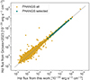 |
Fig. A.2. Comparison between dust-corrected Hα fluxes from Groves et al. (2023) and from our single-region fitting procedure for the 95 selected PHANGS-MUSE H II regions (teal points), as well as for the whole PHANGS-MUSE H II region sample with S/N(Hα) > 5 (golden points). The two fitting procedures produce comparable Hα fluxes, especially for the most brilliant regions (Hα flux ≳5 ⋅ 10−15 erg s−1 cm−2 Å−1) where their relative difference is always < 10%. |
In this appendix we motivate our choice of deriving auroral line fluxes by performing spectral fits in small wavelength regions around the line of interest instead of fitting the entire wavelength range simultaneously. For this comparison, we fit the spectra from the PHANGS–MUSE nebular catalogue using the entire wavelength range and compare the residuals with the fits obtained in Sec. 2.1.1. We focus on on the residuals around the [N II]λ5756, [S III]λ6312 and [O II]λλ7320, 7330 auroral lines. We computed the RMS of residuals over the whole wavelength ranges from Table 1. We only excluded the spectral region at λ ≳ 5775 Å for galaxies observed with ground-layer adaptive optics, as in those objects part of the wavelength range is masked because of the sodium emission of the lasers.
In Fig. A.1 we report the results of RMS computation for our 95 selected H II regions from PHANGS–MUSE nebular catalogue (Sect. 2.1.2). We find systematically higher residual RMS around auroral lines when fitting the entire spectrum. The largest differences in RMS appear around the [N II]λ5756 auroral line, meaning that for this line the two fitting procedures lead to significantly different results, concerning in particular the fit of stellar continuum, as the line fluxes show similar values in both the procedures (with relative differences < 5% in almost all cases).
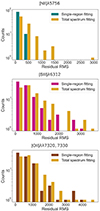 |
Fig. A.1. Histograms describing the distribution of residual RMS around the auroral lines analysed in this work (from left to right: [NII]λ5756, [SIII]λ6312 and [OII]λλ7320, 7330) for the 95 selected H II regions from the PHANGS-MUSE nebular catalogue. The two fitting procedures (single-region and total spectrum) are highlighted with different colours in each panel. |
Some examples comparing the best continuum fits from the two procedures are reported in Figs. A.3 and A.4. In particular, the two H II regions presented in Fig. A.3 are the same as in Fig. 2, while the two H II regions in Fig. A.4 have been selected to illustrate some of the cases where the two different fitting procedures lead to differences of a factor of ≳4 in residual RMS estimates. The presence of an offset between the two fits reflects the fact that the total spectrum fit, as it spans a wavelength range of > 4000 Å, cannot exactly reproduce all the smallest details in restricted wavelength intervals of ∼200 Å as the ones analysed in this work. Interestingly, the bump at λ ∼ 8000 Å evident in the top right panel of Fig. A.4 can be attributed to the presence of Wolf-Rayet (WR) stars within the galaxy and in particular to their broad C IVλ5808 emission (López-Sánchez & Esteban 2010; Monreal-Ibero et al. 2017).
O+ and O2+ chemical abundance measurements for all the catalogues analysed in this work. The asterisk refers to indirect Te estimates using Te-Te relations. In particular, in PHANGS-MUSE analysis Te[O III] is estimated from Eq. 1, while in Nakajima’s analysis Te[N II] is estimated from Te[O III] using the Te-Te relation from Rogers et al. (2021).
The [O II]λλ7320, 7330 auroral lines are the ones that are less influenced by the different adopted fitting procedure. They lie in a region strongly affected by sky lines that lead to high residual RMS in both cases, and the stellar continuum under these lines is rather featureless. Nevertheless, our single-region fitting procedure provides slightly better results, as highlighted in the lower panel of Fig. A.1.
These results demonstrate that single-region fitting provides better stellar continua for the selected spectral regions around auroral lines with respect to total spectrum fitting. There are, however, some issues that could arise when applying this procedure to spectral regions where there is a degeneracy between emission and absorption, for example, around Balmer lines where the stellar absorption becomes significant. To verify that our procedure does not bias the Balmer line fluxes because of incorrect stellar absorption modeling, we compare our measurements of dust-corrected Hα fluxes for both the 95 selected and the whole sample of PHANGS–MUSE H II regions with the same measurements provided by Groves et al. (2023), where total spectrum fitting is instead carried out. The results of this comparison are reported in Fig. A.2. The two fitting procedures always produce comparable Hα fluxes, and the correspondence becomes more precise at higher Hα fluxes, that is, for brighter H II regions. Our 95 selected H II regions all lie within this regime, as they have Hα fluxes ≳7 ⋅ 10−15 erg s−1 cm−2 Å−1: their relative difference between Hα fluxes is always < 10% and in most cases < 5%, which implies variations < 10% in strong-line ratios, negligible with respect to the scatter of the strong-line relations. This suggests that the two procedures provide comparable results, and hence no biases are introduced in Balmer line fitting.
Lastly, we tried to improve the total spectrum fit by increasing the order of the multiplicative polynomial to 12 (from our fiducial value of 8), and we found a marginal improvement in the final fits. However, because our single-region fitting procedure still provides better results and with a lower multiplicative polynomial order, we conclude that this is the best approach to fit the stellar continuum for analysis of this type, where it is not necessary to fit the entire spectrum of a source but it is sufficient to fit with high precision only restricted wavelength regions around the spectral features of interest.
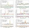 |
Fig. A.3. Comparison between total spectrum and our single-region spectral fitting procedures around the [NII]λ5756 (upper panels), [SIII]λ6312 (middle panels) and [OII]λλ7320, 7330 (lower panels) auroral lines for regions 268 (left column) and 817 (right column) in NGC5068, the same from Fig. 2. When using single-region spectral fitting, the RMS of residuals between data and best-fit around the [NII]λ5756, [SIII]λ6312, and [OII]λλ7320, 7330 lines is respectively of 464, 2781, and 3692 for region 268 and 122, 174, and 420 for region 817. When using total spectrum fitting procedure (golden fits), the RMS of residuals reaches values of 611, 3073 and 3798 for region 268 and 169, 253 and 460 for region 817. The corrected spectral error is represented as a shaded region in the residuals panels. |
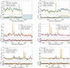 |
Fig. A.4. Two representative examples of H II region spectral fitting around auroral lines where our single-region procedure leads to significantly better results than the standard total spectrum fitting. Left column: region 498 in NGC1566. The RMS of residuals around the [NII]λ5756, [SIII]λ6312 and [OII]λλ7320, 7330 auroral lines (from to bottom) is respectively of 283, 719 and 998 when considering single-region fitting, but reaches values of 1462, 1597 and 1611 when considering total spectrum fitting. For this and the other galaxies observed in AO-WFM, we exclude from RMS evaluation around [NII]λ5756 the wavelength region with λobs ≳ 5775Å, where the flux is masked because of sodium absorption. Right column: region 513 in galaxy NGC5068. In this case, the RMS of residuals around the [NII]λ5756, [SIII]λ6312 and [OII]λλ7320, 7330 auroral lines is respectively of 329, 241, and 1581 when considering single-region fitting, but reaches values of 1489, 1799, and 1933 when considering total spectrum fitting. The corrected spectral error is represented as a shaded region in the residuals panels. |
Appendix B: Temperature and abundance determination for the literature datasets
In this Appendix, we summarise the main differences in the analysis of the literature catalogues with respect to the PHANGS–MUSE data analysis presented in Sects. 3.1 and 3.2. We attempted as far as possible to maintain a homogeneous procedure for determining abundances and temperature, but adaptations were needed due to the differences in line availability.
D.1. Low-redshift data.
In Curti’s (C17) catalogue the main difference from PHANGS-MUSE data is the lack of [S III] lines (Table 3), so that Te[S III] (necessary for estimating sulphur abundance) had to be estimated by exploiting the Te[O III]-Te[S III] relation from Rogers et al. (2021), since Te[O III] can be directly measured. We decided to employ this relation, rather than Eq. 1, for consistency with Nakajima’s catalogue analysis.
In Nakajima’s (N22) catalogue the reported line fluxes allow the measurement of only one electron temperature, Te[O III]. We therefore infer Te[N II] and Te[S III] using the Te[O III]-Te[N II] and Te[O III]-Te[S III] relations from Rogers et al. (2021). The [O II]λ37327, 29 nebular lines are used to infer the O+ abundance.
The CHAOS and Guseva’s (G11) catalogues include all the emission lines present in PHANGS-MUSE. For this two catalogues we therefore carried out the same analysis as for PHANGS–MUSE, even though the availability of additional lines would have allowed a more direct estimate of some quantities (e.g. Te[O III] using [O III]λ4363).
The main difference in the derivation of oxygen ionic abundance estimates are summarised in Table A.1. In three catalogues (CHAOS, C17 and G11) we can measure O+ chemical abundances using both the [O II] auroral and nebular lines. We therefore verified that O+ chemical abundance measurements do not depend on the [O II] lines being used, that is, that we find consistent values by exploiting both nebular and auroral lines. This result is shown in Fig. B.1. Some deviations from the 1:1 relation appear at both high and low metallicities, as it appears from the linear best-fit to the data; however, in these metallicity regimes the limited number of data points makes it challenging to definitively conclude that the two O+ abundance measurements are inconsistent. If present, such inconsistencies may be explained in terms of possible [O II] auroral lines recombination contamination, as observed in Pérez-Montero (2017), and/or different density sensitivity for the auroral and nebular [O II] lines, as proposed in Méndez-Delgado et al. (2023a). In fact, these authors find a median offset of ∼0.1 dex between the two O+ abundance measurements when using [S II]λ6731/λ6716 and [O II]λ3726/λ3729 as density estimators, but this offset disappears when adopting different density-sensitive diagnostics, such as [S II]λλ4069, 4076λλ6716, 6731 or [O II]λλ7320, 7330λλ3726, 3729 (see their Fig. 12). They suggest that this occurs because the [S II]λ6731/λ6716 and [O II]λ3726/λ3729 line ratios do not account for the presence of high-density clumps within the nebulae, introducing a bias of ∼300 cm−2 towards lower densities. This bias particularly affects low-density regions like the ones we are analysing, which typically have ne < 200 cm−2. We do not further explore this hypothesis, as neither the [S II]λλ4069, 4076 nor the [O II]λλ3726, 3729 lines are available for the PHANGS–MUSE H II regions.
In our analysis, we find a median offset between auroral and nebular O+ abundance estimates of ∼0.05 dex, which is slightly lower than what is found in Méndez-Delgado et al. (2023a) and is also lower than the associated errors on both abundance measurements (median error on O+ auroral estimates: ∼0.12 dex; median error on O+ nebular estimates: ∼0.08 dex). Hence, we can conclude that the two estimates are comparable, and therefore we exploit the nebular lines, when available, to minimise the final errors on ionic abundances. Regarding instead the PHANGS–MUSE O+ abundance estimates, which necessarily rely on O+ auroral lines, we find that an eventual offset correction on O+ abundance would produce final oxygen abundances still consistent with the old estimates within the errors (median offset on 12 + log(O/H) of 0.01 dex versus a median error of 0.03 dex). For this reason, we decide not to apply any offset correction.
Another significant difference in data analysis is the adopted temperature estimate for the high ionisation zone. As the [O III]λ4363 auroral line is not available in the PHANGS–MUSE sample, we used the Te[O III]-Te[S III] relation to estimate Te[O III] (Sect. 3.1). We re-calibrated this relation using data from the CHAOS and G11 catalogues, for which both Te[O III] and Te[S III] can be directly measured. We follow a procedure analogue to the one adopted to fit the Te[S III]-Te[N II] relation for PHANGS–MUSE data and we obtain (see Fig. B.2):
![$$ \begin{aligned} T_e [\mathrm{O}\,iii ] = (0.80 \pm 0.02)\, T_e [\mathrm{S}\,{\small {\text{III}}} ] + (0.20 \pm 0.02), \end{aligned} $$](/articles/aa/full_html/2024/11/aa51007-24/aa51007-24-eq16.gif)
with temperatures expressed in units of 104 K. The intrinsic dispersion is σint = 1270 ± 170 K, consistent with what was previously found in Rogers et al. (2021).
We test the use of this Te[O III] on the determination of the O2+ abundance. We find a few data points in both CHAOS and G11 catalogues where the measured Te[O III] is significantly higher than that predicted from the Te[S III]-Te[O III] relation. This trend echoes the findings of Rickards Vaught et al. (2024), who find several regions in PHANGS with abnormally high Te[O III]. In Méndez-Delgado et al. (2023a) similar outliers are not present, and in fact they find a Te[S III]-Te[O III] relation characterised by a smaller intrinsic dispersion of 830 K.
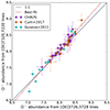 |
Fig. B.1. Comparison between O+ abundances measured using auroral (y axis) and nebular (x axis) lines for CHAOS, C17 and N22 catalogues. |
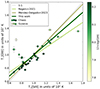 |
Fig. B.2. Te[O III]-Te[S III] relation calibrated over CHAOS and G11 selected data, which are reported with different symbols and colour-coded according to their metallicity. The solid dark green line is the MCMC best-fit relation. For comparison, we also report the Te[O III]-Te[S III] relations from Rogers et al. (2021) and Méndez-Delgado et al. (2023a), and we see that there is a good agreement, especially at lower temperatures that is the physical region covered by the CHAOS sample. The grey line is the 1:1 line. |
D.2. High-redshift data.
Due to the smaller number of emission lines detected and/or reported in high-redshift publications, a significantly different approach was followed to derive temperature and ionic abundances. In particular, dust correction is carried out by exploiting the Hβ/Hγ (λHγ = 4341 Å) ratio fixed at 2.13 rather than Hα/Hβ, as Hα falls out of NIRSpec wavelength coverage at z > 6.6. In both the Laseter et al. (2024) and Sanders et al. (2023) datasets the [O III] nebular and auroral lines are reported, allowing a direct measurement of Te[O III]. [O II] nebular lines are also reported, while [O II] auroral lines are limited to a few detections and some upper limits presented in Sanders et al. (2023), as for numerous galaxies in the sample such emission lines fall outside of NIRSpec wavelength coverage. We thus decided to neglect the [O II] auroral lines in our analysis. Moreover, the [S II]λλ6717, 6731 lines are not reported, so we fixed ne = 300 cm−3, which is a representative value for z = 2 − 3 galaxies (Sanders et al. 2016). As the [N II]λ5756 and [S III]λ6312 auroral lines are not available, we could not estimate either Te[N II] or Te[S III], and hence we had to rely on the direct measurement of Te[O III] and the indirect estimate of Te[O II] (rather than Te[N II], as at high redshift we are dealing only with oxygen lines) from the Te[O III]-Te[O II] relation, as thoroughly described in the reference papers. However, we point out that the use of Te[O II] rather than Te[N II], while referring to the same low-ionisation zone, could introduce some discrepancies (Rogers et al. 2021; Rickards Vaught et al. 2024).
All Tables
Rest-frame wavelength ranges identified for detailed spectral fits, along with the most important emission lines within each region.
Total number of nebulae, along with the number of H II regions meeting the selection criterion individually for each auroral line and simultaneously for all lines, for each galaxy in the PHANGS-MUSE sample.
Temperature estimates and collisionally excited line fluxes used for measuring ionic abundances.
O+ and O2+ chemical abundance measurements for all the catalogues analysed in this work. The asterisk refers to indirect Te estimates using Te-Te relations. In particular, in PHANGS-MUSE analysis Te[O III] is estimated from Eq. 1, while in Nakajima’s analysis Te[N II] is estimated from Te[O III] using the Te-Te relation from Rogers et al. (2021).
All Figures
|
Fig. 1. Spectrum of an H II region (Galaxy: NGC 5068, region ID: 268) with the six spectral regions from Table 1 highlighted in different colours. Auroral lines are the faintest lines of the spectrum, with typical intensities ∼100 times less intense than nebular lines and ∼1000 times less intense than hydrogen recombination lines. |
| In the text | |
|
Fig. 2. Example fits (both stellar continuum and emission lines) of spectral regions around auroral lines for two H II regions in NGC 5068 (IDs: 268 in the upper panels, the same as Fig. 1, and 817 in the lower panels). The [NII]λ5756, [SIII]λ6312 and [OII]λλ7320, 7330 auroral lines are detected with corresponding S/N of 29, 39, 22, and 20 for region 268 and 6, 7, 7, and 7 for region 817. The flux in the y axis is expressed in the same units as Fig. 1. In the lower panels, we additionally report as a shaded region the spectral error band, already re-scaled by the residuals’ standard deviation. |
| In the text | |
|
Fig. 3. Resulting MCMC best fit (in dark green) of the Te[N II]–Te[S III] relation calibrated on PHANGS-MUSE data, which are reported and colour-coded according to their metallicity value (see Sect. 3.2). Other calibrations from previous literature works are reported for comparison; the five curves show comparable behaviours. |
| In the text | |
|
Fig. 4. O+ abundance (upper panel), O2+ abundance (middle panel), and relative ionic abundance of the two species (bottom panel) as a function of the total oxygen abundance for the 95 selected H II regions from the PHANGS-MUSE nebular catalogue. |
| In the text | |
|
Fig. 5. Upper panels: Sulphur and nitrogen chemical abundances versus total system metallicity for the PHANGS–MUSE sample and the other analysed literature catalogues. Lower panels: Relative abundances of sulphur and nitrogen with respect to oxygen, as a function of the total system metallicity. Solar values from Asplund et al. (2009) are reported as teal points for comparison. We display linear trends calibrated either using only the PHANGS-MUSE data or the entire dataset, which also includes literature data. The other log(S/O) versus 12 + log(O/H) trends are from Izotov et al. (2006) and Dors et al. (2016), with the former calibrated over BCD galaxies and the latter over a compilation of literature emission-line intensities of H II regions and star-forming galaxies and while considering sulphur ICF from Thuan et al. (1995). The log(N/O) versus 12 + log(O/H) trend is taken from Nicholls et al. (2017) and it is calibrated over a compilation of literature stellar data. |
| In the text | |
|
Fig. 6. Measurements of ionisation parameter, log(U), for our sample of 95 H II regions. |
| In the text | |
|
Fig. 7. Calibration of R3 = [O III] λ5007/Hβ (panel a), N2 = [N II] λ6584/Hα (panel b), O3N2 = R3/N2 (panel c), and N2S2Hα = N2/S2 ⋅ N20.264 (panel d) diagnostics carried out in this work (solid golden curves). Data points are colour-coded according to the original source catalogues, with golden points associated with PHANGS–MUSE data. The other curves report calibration from the literature for comparison. The dashed extension at low-metallicity shows the extrapolation of our calibrations. |
| In the text | |
|
Fig. 8. Comparison between direct metallicity estimates (x axis) and indirect metallicity estimates (y axis) obtained using the calibration based on R3, N2, O3N2 and N2S2Hα diagnostics proposed in this work. Data points are divided into PHANGS–MUSE data (dark green points) and all the other data taken from the literature catalogues (light green points). The solid line is the 1:1 relation. |
| In the text | |
|
Fig. 9. Dependence of strong-line diagnostics on the ionization parameter. Upper panels: Strong-line diagnostics colour-coded according to the [S III]λλ9069, 9531/[S II]λλ6717, 6731 line ratio. Lower panels: Strong-line diagnostics colour-coded according to the [O III]λ5007/[O II]λλ3726, 3729 line ratio. We have labelled as ‘local’ the data from CHAOS, Curti’s, Guseva’s and Nakajima’s catalogues and as ‘high-z’ data from Sanders et al. (2023) and Laseter et al. (2024). The plotted curves are our diagnostic calibrations plus the high-redshift calibration from Sanders et al. (2023) for R3. |
| In the text | |
|
Fig. 10. Dependence of strong-line ratios on log(U) resulting from the photoionisation model analysis carried out in this work. To realise this figure, in particular, we have analysed a 0.5 Myr SSP input spectrum. Data points are colour-coded according to their log(U) values. |
| In the text | |
|
Fig. 11. 2D metallicity distribution of H II regions in NGC 0628, NGC 1566, NGC 2835 and NGC 4303. H II regions in each galaxy are colour-coded according to their metallicity. Indirect estimates are shown with dots, direct measurements with diamonds. |
| In the text | |
|
Fig. 12. Comparison between indirect metallicity estimates based on our calibration and on PG16, C17 and N22 calibrations (respectively: left, central, and right panels) for all H II regions in the PHANGS–MUSE sample. For each figure, the colourbar describes the contour lines of the metallicity distribution. The solid line indicates the 1:1 relation. |
| In the text | |
|
Fig. 13. Radial metallicity gradients for galaxies NGC 0628, NGC 1566, NGC 2835, and NGC 4303. Metallicity estimates are obtained with our, C17, N22 and PG16 calibrations (from left to right) and reported as small dots in each panel. Big diamonds are the direct measurements, not used to calibrate gradients but reported for visualisation purposes. The solid lines represent the linear best fit performed by excluding data at r < 0.5 reff, and small black dots are the indirect metallicity median values evaluated in 0.36 reff, 0.81 reff, 0.46 reff, and 0.62 reff wide bins, respectively. |
| In the text | |
|
Fig. 14. Comparison between the slopes of metallicity radial gradients fitted on different metallicity estimates based on our PG16 (upper panel), C17 (middle panel), and N22 (lower panel) calibrations. The solid line is the 1:1 relation. For visual clarity, we have highlighted with different colours the four galaxies from Fig. 11. |
| In the text | |
|
Fig. A.2. Comparison between dust-corrected Hα fluxes from Groves et al. (2023) and from our single-region fitting procedure for the 95 selected PHANGS-MUSE H II regions (teal points), as well as for the whole PHANGS-MUSE H II region sample with S/N(Hα) > 5 (golden points). The two fitting procedures produce comparable Hα fluxes, especially for the most brilliant regions (Hα flux ≳5 ⋅ 10−15 erg s−1 cm−2 Å−1) where their relative difference is always < 10%. |
| In the text | |
|
Fig. A.1. Histograms describing the distribution of residual RMS around the auroral lines analysed in this work (from left to right: [NII]λ5756, [SIII]λ6312 and [OII]λλ7320, 7330) for the 95 selected H II regions from the PHANGS-MUSE nebular catalogue. The two fitting procedures (single-region and total spectrum) are highlighted with different colours in each panel. |
| In the text | |
|
Fig. A.3. Comparison between total spectrum and our single-region spectral fitting procedures around the [NII]λ5756 (upper panels), [SIII]λ6312 (middle panels) and [OII]λλ7320, 7330 (lower panels) auroral lines for regions 268 (left column) and 817 (right column) in NGC5068, the same from Fig. 2. When using single-region spectral fitting, the RMS of residuals between data and best-fit around the [NII]λ5756, [SIII]λ6312, and [OII]λλ7320, 7330 lines is respectively of 464, 2781, and 3692 for region 268 and 122, 174, and 420 for region 817. When using total spectrum fitting procedure (golden fits), the RMS of residuals reaches values of 611, 3073 and 3798 for region 268 and 169, 253 and 460 for region 817. The corrected spectral error is represented as a shaded region in the residuals panels. |
| In the text | |
|
Fig. A.4. Two representative examples of H II region spectral fitting around auroral lines where our single-region procedure leads to significantly better results than the standard total spectrum fitting. Left column: region 498 in NGC1566. The RMS of residuals around the [NII]λ5756, [SIII]λ6312 and [OII]λλ7320, 7330 auroral lines (from to bottom) is respectively of 283, 719 and 998 when considering single-region fitting, but reaches values of 1462, 1597 and 1611 when considering total spectrum fitting. For this and the other galaxies observed in AO-WFM, we exclude from RMS evaluation around [NII]λ5756 the wavelength region with λobs ≳ 5775Å, where the flux is masked because of sodium absorption. Right column: region 513 in galaxy NGC5068. In this case, the RMS of residuals around the [NII]λ5756, [SIII]λ6312 and [OII]λλ7320, 7330 auroral lines is respectively of 329, 241, and 1581 when considering single-region fitting, but reaches values of 1489, 1799, and 1933 when considering total spectrum fitting. The corrected spectral error is represented as a shaded region in the residuals panels. |
| In the text | |
|
Fig. B.1. Comparison between O+ abundances measured using auroral (y axis) and nebular (x axis) lines for CHAOS, C17 and N22 catalogues. |
| In the text | |
|
Fig. B.2. Te[O III]-Te[S III] relation calibrated over CHAOS and G11 selected data, which are reported with different symbols and colour-coded according to their metallicity. The solid dark green line is the MCMC best-fit relation. For comparison, we also report the Te[O III]-Te[S III] relations from Rogers et al. (2021) and Méndez-Delgado et al. (2023a), and we see that there is a good agreement, especially at lower temperatures that is the physical region covered by the CHAOS sample. The grey line is the 1:1 line. |
| In the text | |
Current usage metrics show cumulative count of Article Views (full-text article views including HTML views, PDF and ePub downloads, according to the available data) and Abstracts Views on Vision4Press platform.
Data correspond to usage on the plateform after 2015. The current usage metrics is available 48-96 hours after online publication and is updated daily on week days.
Initial download of the metrics may take a while.