| Issue |
A&A
Volume 659, March 2022
|
|
|---|---|---|
| Article Number | A17 | |
| Number of page(s) | 23 | |
| Section | Planets and planetary systems | |
| DOI | https://doi.org/10.1051/0004-6361/202142653 | |
| Published online | 02 March 2022 | |
Discovery and mass measurement of the hot, transiting, Earth-sized planet, GJ 3929 b★
1
Landessternwarte, Zentrum für Astronomie der Universität Heidelberg,
Königstuhl 12,
69117
Heidelberg,
Germany
e-mail: This email address is being protected from spambots. You need JavaScript enabled to view it.
2
Institut für Astrophysik, Georg-August-Universität,
Friedrich-Hund-Platz 1,
37077
Göttingen,
Germany
3
Max-Planck-Institut für Astronomie,
Königstuhl 17,
69117
Heidelberg,
Germany
4
Centro de Astrobiología (CSIC-INTA), ESAC, Camino bajo del castillo s/n,
28692
Villanueva de la Cañada,
Madrid,
Spain
5
Instituto de Astrofísica de Andalucía (CSIC), Glorieta de la Astronomía s/n,
18008
Granada,
Spain
6
Center for Astrophysics | Harvard & Smithsonian,
60 Garden Street,
Cambridge,
MA
02138,
USA
7
Space Telescope Science Institute,
Baltimore,
MD
21218,
USA
8
Institut de Ciències de l’Espai (ICE, CSIC),
Campus UAB, c/ de Can Magrans s/n,
08193
Cerdanyola del Vallès,
Spain
9
Institut d’Estudis Espacials de Catalunya (IEEC),
c/ Gran Capità 2-4,
08034
Barcelona,
Spain
10
NASA Ames Research Center,
Moffett Field,
CA
94035,
USA
11
Komaba Institute for Science, The University of Tokyo,
3-8-1 Komaba,
Meguro,
Tokyo
153-8902,
Japan
12
Astrobiology Center,
2-21-1 Osawa,
Mitaka,
Tokyo
181-8588,
Japan
13
Instituto de Astrofísica de Canarias (IAC),
38205
La Laguna,
Tenerife,
Spain
14
Departamento de Astrofísica, Universidad de La Laguna,
38206
La Laguna,
Tenerife,
Spain
15
Department of Physics and Kavli Institute for Astrophysics and Space Research, Massachusetts Institute of Technology,
Cambridge,
MA
02139,
USA
16
Department of Earth, Atmospheric and Planetary Sciences, Massachusetts Institute of Technology,
Cambridge,
MA
02139,
USA
17
Department of Aeronautics and Astronautics, Massachusetts Institute of Technology,
77 Massachusetts Avenue,
Cambridge,
MA
02139,
USA
18
Center for Space and Habitability, University of Bern,
Gesellschaftsstrasse 6,
3012,
Bern,
Switzerland
19
Department of Astrophysical Sciences, Princeton University,
4 Ivy Lane,
Princeton,
NJ
08544,
USA
20
NASA Goddard Space Flight Center,
8800 Greenbelt Road,
Greenbelt,
MD
20771,
USA
21
University of Maryland,
Baltimore County, 1000 Hilltop Circle,
Baltimore,
MD
21250,
USA
22
Thüringer Landessternwarte Tautenburg,
Sternwarte 5,
07778
Tautenburg,
Germany
23
George Mason University,
4400 University Drive,
Fairfax,
VA
22030,
USA
24
Universidad Nacional Autónoma de México, Instituto de Astronomía,
AP 70-264,
CDMX
04510,
Mexico
25
Centro Astronónomico Hispano Alemán, Observatorio de Calar Alto, Sierra de los Filabres,
04550
Gérgal,
Spain
26
Department of Astronomy and Tsinghua Centre for Astrophysics, Tsinghua University,
Beijing
100084,
PR China
27
Astrobiology Research Unit, Université de Liège,
Allée du 6 Août 19C,
4000
Liège,
Belgium
28
Max-Planck-Institut für Sonnensystemforschung,
Justus-von-Liebig Weg 3,
37077
Göttingen,
Germany
29
Department of Physics, University of Warwick,
Gibbet Hill Road,
Coventry
CV4 7AL,
UK
30
Universitäts-Sternwarte, Ludwig-Maximilians-Universität München,
Scheinerstrasse 1,
81679
München,
Germany
31
Exzellenzcluster Origins,
Boltzmannstraße 2,
85748
Garching,
Germany
32
Departamento de Física de la Tierra y Astrofísica & IPARCOS-UCM (Instituto de Física de Partículas y del Cosmos de la UCM), Facultad de Ciencias Físicas, Universidad Complutense de Madrid,
28040
Madrid,
Spain
33
Hamburger Sternwarte,
Gojenbergsweg 112,
21029
Hamburg,
Germany
34
Homer L. Dodge Department of Physics and Astronomy, University of Oklahoma,
440 West Brooks Street,
Norman,
OK
73019,
USA
35
Universidad Nacional Autónoma de México, Instituto de Astronomía,
AP 106,
Ensenada
22800,
BC,
Mexico
36
Patashnick Voorheesville Observatory,
Voorheesville,
NY
12186,
USA
37
SETI Institute,
Mountain View,
CA
94043,
USA
38
Vereniging Voor Sterrenkunde, Brugge, Belgium & Centre for mathematical Plasma-Astrophysics, Department of Mathematics, Katholieke Universiteit Leuven,
Celestijnenlaan 200B,
3001
Heverlee,
Belgium
39
AstroLAB IRIS, Provinciaal Domein “De Palingbeek”,
Verbrandemolenstraat 5,
8902
Zillebeke,
Ieper,
Belgium
Received:
12
November
2021
Accepted:
13
January
2022
Abstract
We report the discovery of GJ 3929 b, a hot Earth-sized planet orbiting the nearby M3.5 V dwarf star, GJ 3929 (G 180-18, TOI-2013). Joint modelling of photometric observations from TESS sectors 24 and 25 together with 73 spectroscopic observations from CARMENES and follow-up transit observations from SAINT-EX, LCOGT, and OSN yields a planet radius of Rb = 1.150 ± 0.040 R⊕, a mass of Mb = 1.21 ± 0.42 M⊕, and an orbital period of Pb = 2.6162745 ± 0.0000030 d. The resulting density of ρb = 4.4 ± 1.6 g cm−3 is compatible with the Earth’s mean density of about 5.5 g cm−3. Due to the apparent brightness of the host star (J = 8.7 mag) and its small size, GJ 3929 b is a promising target for atmospheric characterisation with the JWST. Additionally, the radial velocity data show evidence for another planet candidate with P[c] = 14.303 ± 0.035 d, which is likely unrelated to the stellar rotation period, Prot = 122 ± 13 d, which we determined from archival HATNet and ASAS-SN photometry combined with newly obtained TJO data.
Key words: planetary systems / techniques: radial velocities / techniques: photometric / stars: individual: GJ 3929 / stars: late-type / planets and satellites: detection
RV data and stellar activity indices are only available at the CDS via anonymous ftp to cdsarc.u-strasbg.fr (130.79.128.5) or via http://cdsarc.u-strasbg.fr/viz-bin/cat/J/A+A/659/A17
Fellow of the International Max Planck Research School for Astronomy and Cosmic Physics at the University of Heidelberg (IMPRS-HD).
© ESO 2022
1 Introduction
The Transiting Exoplanet Survey Satellite (TESS; Ricker et al. 2015) has led to the discovery and characterisation of a multitude of small exoplanets. This growth was facilitated by the intensive spectroscopic follow-up in order to measure radial velocities (RVs) of the TESS objects of interest (TOI; Guerrero et al. 2021) and, thus, confirm their planetary nature by measuring their masses. (e.g. Cloutier et al. 2019; Günther et al. 2019; Luque et al. 2019; Astudillo-Defru et al. 2020; Dreizler et al. 2021; Kemmer et al. 2020; Nowak et al. 2020; Stefánsson et al. 2020; Soto et al. 2021; Bluhm et al. 2020, 2021). These discoveries provide valuable data in the ongoing debate as to the origins of super-Earths and mini-Neptunes.
The so-called radius gap, first observationally shown by Fulton et al. (2017), divides the transiting sub-Neptunian planets into two different populations. Complementary mass measurements for planets on both sides of the gap confirmed their differing nature: dense and presumably rocky super-Earths with smaller radii and low-density enveloped mini-Neptunes with larger radii (e.g. Rogers 2015; Jontof-Hutter 2019; Bean et al. 2021, and references therein). However, it is not clear which formation mechanisms lead to these distinct planet types.
For example, rocky super-Earths could be created by photo-evaporation (Owen & Wu 2013, 2017) or core-powered mass loss (Ginzburg et al. 2018; Gupta & Schlichting 2019) of mini-Neptunes with hydrogen-dominated atmospheres. The upper radius and mass limit of the rocky planets and its dependency on the planet’s period, or rather instellation, are often seen as evidence for this theory (e.g. van Eylen et al. 2018, 2021; Bean et al. 2021, and references therein). On the other hand, the growing number of planets residing in the gap pose a challenge to this, since their high instellation usually excludes substantial H-He atmospheres (e.g. Ment et al. 2019; Dai et al. 2019; Bluhm et al. 2020). A possible explanation would be the existence of “water planets”, which were predicted by classical planet formation models (e.g. Bitsch et al. 2019). In fact, self-consistent planet formation models, such as those by Venturini et al. (2020a,b), predict a bimodal distribution, with purely rocky planets on one side and water-enriched planets on the other. Probing the atmospheres of mini-Neptunes will break the density degeneracy between H-He atmospheres and water planets and provide more insight (Rogers & Seager 2010; Lopez & Fortney 2014; Zeng et al. 2019). The position of the radius gap, anchored by the distribution of planets on both sides, is also a probe for the underlying principles and an important input for theoretical models that aim to describe the formation and evolution of those planets (Bean et al. 2021 and references therein).
Considered on their own, the planets below the radius gap are also interesting. For example, the increasing statistical sample of the smallest planets will tell us if super-Earths are different from planets with masses and radii similar to Earth, or if the underlying formation mechanisms are the same. Related to this is the question how abundant atmosphereswith high mean-molecular-weight similar to the ones that we observe in the Solar System actually are. Particularly suited to answer those questions are the planets orbiting M-dwarf stars, as these will be the first ones where the atmospheric characterisation of exo-Earths will be possible and provide unique insight in their structure and composition (e.g. Rauer et al. 2011; Barstow & Irwin 2016; Morley et al. 2017; Kempton et al. 2018).
In this study, we present the discovery of a hot Earth-sized planet orbiting the M3.5 V-dwarf star, GJ 3929. Based on transit signals observed by TESS, we performed an intensive RV follow-up campaign with CARMENES to confirm its planetary origin. The characterisation of the planet was supported by photometric follow-up from SAINT-EX, LCOGT, and OSN that helped to refine the transit parameters. Furthermore, we report the detection of a non-transiting, sub-Neptunian-mass planet candidate with a wider orbit, which is evident in the RV data.
Our paper is organised as follows. In Sect. 2, we present the data used, and in Sect. 3 we describe the stellar properties of GJ 3929. Data analysis is described in Sect. 4, and our findings are discussed in Sect. 5. Finally, Sect. 6 gives a summary of our results.
Summary of transit observations.
2 Data
2.1 High-resolution spectroscopy
We took 78 observations of GJ 3929 between July 2020 and July 2021 with CARMENES1 (Quirrenbach et al. 2014) in the course of the guaranteed time observation and legacy programmes. The dual-channel spectrograph covers the spectral ranges of 0.52 μm–0.96 μm in the visible light (VIS;  ) and 0.96 μm1.71 μm in the near infrared (NIR;
  ). For the data reduction and extraction of the RVs, we used caracal (Caballero et al. 2016b) and serval (Zechmeister et al. 2018, 2020), following our standard approach (e.g. Kemmer et al. 2020). The observations were taken with an exposure time of 30 min, which resulted in a median signal-to-noise ratio (S/N) of 74 (min. = 15, max. = 100). After discarding spectra with missing drift correction (i.e. without simultaneous calibration measurements from the Fabry-Pérot), we retrieved 73 RVs in the VIS with a median internal uncertainty of 1.9 m s−1 and a weighted root mean square (wrms) of 4.0 m s−1 and 72 RVs in the NIR with a median internal uncertainty of 7.3 m s−1 and wrms 9.1 m s−1 in the NIR, respectively. Due to the large scatter of the NIR data and the small expected amplitude of the transiting planet candidate, we only considered the VIS data in our analysis (Bauer et al. 2020).
2.2 Transit photometry
For our analysis, we combined the TESS observations with ground based follow-up transit photometry obtained by the TESS follow-up observing programme sub-group one. The parameters of the used transit observations are summarised in Table 1. In the following, we provide an overview of the instruments and applied data reduction.
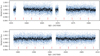 |
Fig. 1 TESS PDCSAP light curves for sector 24 (top) and sector 25 (bottom). The blue points are the measurements and the black dots are 20 min bins. The transit times of GJ 3929 b are indicated by red ticks. |
2.2.1 TESS
We retrieved TESS observations for GJ 3929 (TOI 2013) from the Mikulski Archive for Space Telescopes2 for the two sectors 24 and 25 (see Fig. 1). In sector 24 (camera #1, CCD #1), one transit event was not observed because of the interruption during the data downlink between BJD = 2458968.35 and BJD = 2458969.27. In sector 25(Camera #1, CCD #2), the measurements were stopped for data download between BJD = 2458995.63 and BJD = 2458996.91, which led to one, only partially observed, transit. We used the pre-search data conditioning simple aperture photometry (PDCSAP; Smith et al. 2012; Stumpe et al. 2012, 2014) light curves provided by the Science Processing Operations Center (SPOC; Jenkins et al. 2016), which are based on simple aperture photometry (SAP) light curves, but further corrected for instrument characteristics. The aperture masks used for retrieving the SAP light curves are shown in Fig. 2. To reduce the computational cost of the analysis, we used the extracted transit events only. In doing so, the baseline for each transit was set to ± 3 h with respect to the expected times of transit centre.
2.2.2 SAINT-EX
The first follow-up transit photometry for GJ 3929 was taken with the SAINT-EX3 telescope located at the Observatorio Astronómico Nacional in the Sierra de San Pedro Mártir in Baja California, Mexico. SAINT-EX consists of an Andor iKon-L camera mounted to an 1 m f∕8 Ritchey–Chrétien telescope with a pixel scale of 0′′.34 pix−1, which corresponds to a field of view (FOV) of 12′× 12′ (Demory et al. 2020). The reduction of the data was performed using the instrument’s custom pipeline, prince, which performs the standard image reduction steps including bias, dark, and flat-field correction and provides light curves obtained from differential photometry (Demory et al. 2020). The light curve used for our analysis was further corrected for systematics using a principle component analysis (PCA) method based on the light curves of all suitable stars in the FOV except for the target star (Wells et al. 2021).
2.2.3 LCOGT
Two transit events were observed with instruments from the LCO4 global telescope network (LCOGT; Brown et al. 2013). The first one was observed contemporaneously by the SINISTRO CCDs at the 1 m telescopes of the McDonald Observatory (McD) and the Cerro Tololo Interamerican Observatory (CTIO). Both instruments have a pixel scale of 0′′.389 pix−1 and a FOV of 26′× 26′. However, the higher airmass at LCOGT CTIO (see Table 1) led to worse seeing (estimated point spread function size 5′′.34 pix−1 vs. 3′′.97 pix−1) and, therefore, larger scatter of the measurements. The second transit event was observed by the recently commissioned MuSCAT35 camera (Narita et al. 2020) mounted on the 2 m Faulkes Telescope North at Haleakalā Observatory (HAL). MuSCAT3 operates simultaneously in the four passbands, g′, r′, i′, and  and has a pixel scale of 0′′.27 pix−1 corresponding to a FOV of 9.′1 × 9.′1. All LCOGT observations were calibrated by the standard LCOGT BANZAI pipeline (McCully et al. 2018a,b), and photometric data were extracted using AstroImageJ (Collins et al. 2017).
2.2.4 OSN
We detected four transit events with the 90 cm Ritchey–Chrétien telescope of the Observatorio de Sierra Nevada (OSN). The telescope is equipped with a 2k × 2k CCD camera with a pixel scale of 0′′.4 pix−1 that provides a FOV of 13.′2 × 13.′2 (Amado et al. 2021). All frames were corrected for bias and flat-fielding, and the light curves were obtained using synthetic aperture photometry. Outliers due to bad weather or very high airmass were removed from the dataset. The light curves were de-trended before the fitting using the airmass in a linear fit.
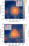 |
Fig. 2 TESS TPFs of GJ 3929. Top: TESS sector 24, bottom: TESS sector 25. The position of GJ 3929 is denoted by a white cross, and the aperture mask used to create the PDCSAP light curves is shown as the pixels with orange borders. For comparison, nearby sources from the Gaia DR2 catalogue (Gaia Collaboration 2018), up to a difference of Δm = 8 mag in brightness compared to GJ 3929, are plotted by red circles. Figure created using tpfplotter (Aller et al. 2020). |
2.3 Long-term photometry
In addition to the photometric transit observations, we used long-term photometry to determine the stellar rotation period.
2.3.1 HATNet
The photometric variability of GJ 3929 was previously investigated by Hartman et al. (2011) using data from the HATNet telescope network (Bakos et al. 2004, 2006). HATNet comprises a network of six cameras attached to 11 cm telescopes located in Arizona and Hawai’i. The cameras have a FOV of 8°. 2 ×8°.2 and a pixel scale of 14′′ pix−1. We retrieved the observations covering a time span of 200 d between December 2004 and July 2005 from the NASA Exoplanet Archive6. The data were taken by telescopes #9 and #11 in the Cousins Ic filter at the Fred Lawrence Whipple Observatory in Arizona. Originally, the data were taken with a cadence of 5.5 min, but for our search for long-periodic signals we used the nightly binned values. In this way, we obtain a mean uncertainty of 1.24 ppt and rms of 2.19 ppt.
2.3.2 ASAS-SN
We obtained more than 5 yr of archival data from ASAS-SN (Shappee et al. 2014; Kochanek et al. 2017), which were taken between April 2013 and September 2018. ASAS-SN currently consists of 24 cameras mounted on the 14 cm Nikon telephoto lenses at six different sites around the globe. Each unit has a FOV of 4°. 5 × 4°.5 with a pixel scale of 8′′.0 pix−1. The observations of GJ 3929 were obtained in the V band with the second camera in Hawai’i and have a mean uncertainty of 4.82 ppt and rms of 6.68 ppt.
2.3.3 TJO
We observed GJ 3929 from April to October 2021 with the 0.8 m Joan Oró telescope (TJO; Colomé et al. 2010) at the Montsec Observatory in Lleida, Spain. We obtained a total of 593 images with an exposure time of 60 s using the Johnson R filter of the LAIA imager, a 4k ×4k CCD with a field of view of 30′ and a scale of 0′′.4 pix−1. The images were calibrated with darks, bias, and flat fields with the icat pipeline of the TJO (Colome & Ribas 2006). The differential photometry was extracted with AstroImageJ using the aperture size that minimised the rms of the resulting relative fluxes, and a selection of the ten brightest comparison stars in the field that did not show variability. Then, we used our own pipelines to remove outliers and measurements affected by poor observing conditions or presenting a low signal-to-noise ratio. For our analysis, we binned the data nightly, which resulted in a total of 54 measurements with a mean uncertainty of 1.90 ppt and rms of 6.22 ppt.
2.4 High-resolution imaging
We observed GJ 3929 with the high-spatial resolution camera AstraLux (Hormuth et al. 2008), which is located at the 2.2 m telescope of the Calar Alto Observatory (Almería, Spain). The observations were carried out on 7 August 2020 at an airmass of 1.1 and under moderate weather conditions with a mean seeing of 1′′.1. In total, we obtained 93 700 frames in the Sloan Digital Sky Survey z′ filter (SDSSz) with 10 ms exposure times and windowed to a FOV of 6′′ × 6′′. We used theinstrument pipeline to select the 10 % frames with the highest Strehl ratio (Strehl 1902) and to combine them into a final high-spatial-resolution image. Based on this final image, a sensitivity curve was computed using our own developed astrasens7 package (Lillo-Box et al. 2012, 2014).
3 Properties of GJ 3929
The star GJ 3929 (G 180-18, Karmn J15583+354) is located at a distance of only 15.830 ± 0.006 pc and shows a high proper motion (Schneider et al. 2016; Gaia Collaboration 2018). Lépine et al. (2013) classified the star as an M3.5 V red dwarf. We calculated homogeneous stellar parameters from the CARMENES high-resolution spectra using our standard method: the luminosity, L⋆ = 0.01155 ± 0.00011 L⊙, was determined in Cifuentes et al. (2020). Following Passegger et al. (2019), and assuming v sin i = 2 km s−1, we derived the effective temperature, Teff = 3369 ± 51 K, surface gravity logg = 4.84 ± 0.04 dex, and metallicity [Fe∕H] = 0.00 ± 0.16 dex using the VIS spectra8. Finally, we computed the stellar radius, R⋆ = 0.315 ± 0.010 R⊙, using the Stefan-Boltzman law, and, consequentially, the mass, M⋆ = 0.309 ± 0.014 R⊙, from the empirical mass-radius relation for M dwarfs of Schweitzer et al. (2019). Additionally, we computed galactocentric space velocities UV W as in Cortés-Contreras (2017).
From the analysis of the Hα pseudo-equivalent width (pEW), we found that GJ 3929 is an Hα-inactive star and is consistent with the previous results of Schöfer et al. (2019) and Jeffers et al. (2018). In addition, we investigated if there are any correlations between the measured CARMENES RV values and all of the activity indices using the Pearson’s r coefficient where a value of >0.7 or <−0.7 indicates strong correlation or anti-correlation as previously described by Jeffers et al. (2020). We found no strong or even moderate correlations between the measured CARMENES RVs and the activity indices, confirming that GJ 3929 is a magnetically inactive star. In Sect. 4.7, we present a combined analysis of CARMENES activity indicators and photometry from HATNet, ASAS-SN, and TJO, from which we determine a stellar rotation period of 122 ± 13 d.
GJ 3929 has no known stellar companions. From the high-resolution imaging presented in Sect. 4.2, we can rule out companions up to contrasts of Δm = 4 mag down to a separation of 0′′.2 and Δm = 5.5 mag for separations of 0′′.4 to 2′. Additionally, Gaia provides a re-normalised unit weight error of 1.19, which is below the critical value of 1.41 that would hint to a close companion. Besides this, we complemented the multiplicity analysis with a wide common-proper-motion companion search with Gaia EDR3 data up to a projected physical separation of 105 au (over 10 arcmin in angular separation); no wide companions with similar parallax and proper motion were found. Furthermore, the astrometric excess-noise is 0.22 mas, which is consistent with the jitter of other sources with comparable G magnitudes between 11 mag to 13 mag. Our RV analysis in Sect. 4.5 also shows no signals that would indicate any massive companions. A summary of the compiled stellar parameters and their sources is provided in Table 2.
4 Analysis and results
4.1 Transit detection by the SPOC
The SPOC investigated the PDCSAP flux time series for sector 24 with the Transiting Planet Search (Jenkins et al. 2002, 2010, 2020) module using an adaptive, wavelet-based matched filter, which detected transit events with a period of ~ 2.6 d and generated a “threshold crossing event”. The data were fitted with an initial limb-darkened transit model (Li et al. 2019) and subjected to a suite of diagnostic tests to help elucidate the nature of the signal (Twicken et al. 2018). The transit signal passed all the tests in the data validation module, and it was promoted from ‘threshold crossing event’ to TOI status by the TESS Science Office on 19 June 2020 after reviewing the Data Validation reports (Guerrero et al. 2021). Subsequent joint analyses of sectors 24 and 25 indicated that the transit source is located within 2′′.8± 6′′.6 of GJ 3929. The multiple transiting planet search failed to identify any additional transiting planet signatures.
Stellar parameters of GJ 3929.
4.2 Limits of photometric contamination
As seen in Fig. 2, there are no Gaia sources down to a brightness difference of ΔG ≈ 7 mag within the apertures used for creating the SAP light curves. The SPOC estimated a contamination in the photometric aperture of about 0.4% for both sectors, based on the crowding and the location of the target star on the CCD using the pixel response functions reconstructed from data collected during commissioning and early science operations. Nevertheless, we obtained additional lucky imaging observations to rule out contamination of the light curves by bound or unbound companions at sub-arcsecond separations (Sect. 2.4). The AstraLux image of GJ 3929 and the contrast curve created from it are shown in Fig. 3. We find no evidence of additional sources within this FOV and within the computed sensitivity limit. This allows us to set an upper limit to the contamination in the light curve of around 0.4% down to 0′′.4 and 2.5% down to 0′′.2.
Analogously to Lillo-Box et al. (2014), we further used the contrast curve to estimate the probability of contamination from blended sources in the TESS aperture based on the TRILEGAL9 Galactic model (v1.6, Girardi et al. 2012). The transiting planet candidate around GJ 3929 produces a signal that could be mimicked by blended eclipsing binaries with magnitude contrasts up to Δmb,max ≈ 7.3 mag in the SDSSz passband. Translating this contrast results in a low probability of 0.1% for an undetected source, and an even lower probability of such a source being an appropriate eclipsing binary. Given these numbers, we assumed that the transit signal is not due to a blended binary star and that the probability of a contaminating source is nearly zero.
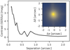 |
Fig. 3 Contrast curve of the AstraLux high-resolution image. The image used to create the contrast curve is shown in the inset. |
4.3 Modelling technique
We used juliet10 (Espinoza et al. 2019) for the analysis and modelling of the transit and RV data. Thereby, we follow our method as detailed for example by Luque et al. (2019), Kemmer et al. (2020), or Stock et al. (2020b). Because of the variety of instruments used and the large dataset, it would not be reasonable to perform the model selection on the combined RV and transit data. Therefore, in the following we first present transit-only and RV-only analyses to determine the individually best fitting models, which were later combined into a joint fit to retrieve the most precise parameters for the system.
4.4 Transit-only modelling
In the first step of the modelling, we combined the TESS light curves with the SAINT-EX, LCOGT, and OSN follow-up transits to obtain a very precise updated ephemeris of the transiting planet candidate, which was later used as prior information for the RV-only modelling.
Planet parameters
Based on the analysis of the TESS light curves by the SPOC pipeline (Li et al. 2019), the transiting planet candidate has a period of 2.616277 ± 0.000113 d. We used this information to set a uniform prior between 2 d to 3 d for our analysis. The time-of-transit centre was chosen accordingly to be uniform between BJD 2459319.0 d to 2459322.0 d, which comprises the decently resolved follow-up transit observed by LCOGT-HAL. Following our usual approach (e.g. Luque et al. 2019; Kemmer et al. 2020; Bluhm et al. 2021), we fitted for the stellar density, ρ*, instead of the scaled planetary semi-major axis, a∕R*. In doing so, we used a normally distributed prior centred on the density calculated from the parameters in Table 2. For this, we assigned a width of three times the propagated uncertainty. Furthermore, we implemented the re-parameterised fit variables r1 and r2, which replace the planet-to-star radius ratio, p, and the impact parameter, b, and allow for a uniform sampling between zero and one (Espinoza 2018). Since the information content regarding the eccentricity is rather small for the light curves (Barnes 2007; Kipping 2008; van Eylen & Albrecht 2015), we assumed it to be zero for the transit-only modelling. Constraints on the eccentricity were later investigated using the RV data (see Sect. 4.5).
Instrument parameters
The analysis of the high-resolution images (Sect. 4.2) did not indicate any contaminating sources within the apertures that were used to generate the light curves. Therefore, the dilution factor was fixed to 1 for all instruments. Following Espinoza & Jordán (2015), we used a quadratic limb-darkening law for the space-based TESS light curves, parameterised by q1 and q2 as in Kipping (2013). The parameters were shared between the two sectors. For all the other ground-based follow-up observations, we assumed a linear limb darkening with coefficient q. The offsets between the instruments, mflux, were assumed to be normally distributed around 0 with a standard deviation of 0.1, whereas the additional scatter that was added in quadrature to the nominal uncertainty values was log-uniformly distributed between 0 ppm to 5000 ppm. The light curves from the LCOGT were de-trended simultaneously with the fits, whereas, following a preliminary analysis, de-trending of the SAINT-EX light curve did not bring any improvement, which is why we refrained from doing so in the analysis. Moreover, the OSN light curves were de-trended before the fit as described inSect. 2.2. We invite the reader to consult Table 1 for an overview of the used de-trending parameters of the individual light curves. In this way, we determined a refined period of P = 2.6162733 ± 0.0000034 d and t0 = 2459320.05803 ± 0.00024 d from the fit.
In order to search for additional transit signals in the data, we applied the model from this fit to the entire TESS dataset (i.e. uncropped) and ran a transit least squares (TLS; Hippke & Heller 2019) periodogram on the residuals. The periodogram did not show any further significant signals.
4.5 RV-only modelling
4.5.1 Periodogram analysis
We used generalised Lomb-Scargle periodograms (GLS; Zechmeister & Kürster 2009) implemented in Exo-Striker (Trifonov 2019; Trifonov et al. 2021) to identify prominent signals in the RV data, as illustrated by Fig. 4. The dominant period is not that of the transiting planet candidate at about 2.6 d, but a signal with periodicity of P ≈ 15 d and its one-day aliases. Furthermore, aliasing due to the seasonal observability of GJ 3929 (fs ≈ 1∕292 d−1) splits the ~15-day signal up into multiple close peaks by itself. The two prominent peaks are thereby at periods of P ≈ 14.3 d and P ≈ 15.0 d (see also Sect. 4.5.2). As there are no obvious indications of a transiting signal corresponding to these two periodicities that would help to distinguish the aliases, we used a sinusoidal fit with an uninformative period boundary between 10 d to 20 d to subtract the signal, and determined a period of P = 15.03 d. The residuals of this fit show a peak with about a 2% false alarm probability (FAP) at a period of P ≈ 1.62 d. This period corresponds to the one-day alias of the 2.62-day signal seen in the transits, which is itself apparent only as an insignificant signal in the GLS periodogram. The photometric observations presented in the previous section, however, supplied precise information on the period and transit time, and hence phase, of the transiting planet candidate. We therefore simultaneously fitted the ~15-day signal in combination with a sinusoid of P ≈ 2.62 d, whose ephemeris was fixed to the values from Sect. 4.4. The residuals of this fit do not show any power at the period of P ≈ 1.62 d, which confirms that the peak is indeed correlated in phase with the signal of the transiting planet candidate, and, thus, it is caused by aliasing. Even though never significant, a peak near the stellar rotation period of 122 d is also visible in the GLS periodograms (see Sect. 4.7).
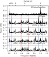 |
Fig. 4 GLS periodogram analysis of the RVs. In the first panel, we show the window function of the CARMENES data. In the subsequent panels, the residuals after subtracting models of increasing complexity are presented. The components that were considered for the fits are listed in the inset texts (see also Table 3). The period, P = 2.62 d, and one-day alias, P = 1.62 d, of the transiting planet are marked by the red solid and dashed lines, while the ~ 15-day periodicity and its daily aliases are marked by blue solid and dashed lines, respectively. Additionally, even though insignificant in the periodogram, the stellar rotation period of P = 122 d (Sect. 4.7) is indicated by the purple dot-dashed line. We normalised the power using the parametrisation of Zechmeister & Kürster (2009), and the 10, 1, and 0.1% FAPs denoted by the horizontal grey dashed lines were calculated using the analytic expression. |
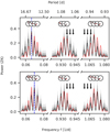 |
Fig. 5 Alias test for the 14.3-day and 15.0-day periods using AliasFinder. We generated 5000 synthetic datasets for each period to produce synthetic periodograms (black lines), which are compared with the periodogram of the observed data (red lines). The simulation for the 15.0-day signal is shown in the top row and the simulation for the 14.3-day signal in the bottom row, each period indicated by a vertical blue dashed line, respectively. Black lines depict the median of the samples for each simulation, and the grey shaded areas are the 50, 90, and 99% confidence intervals. Furthermore, the phases of the peaks as determined by the GLS periodogram are displayed in the circles, following the same colour scheme (the grey shades denote the standard deviations of the simulated peaks). The black arrows point out the difference in the periodograms for the daily aliases that allows to identify the best matching period (see the text for the discussion). |
4.5.2 Determining the true period underlying the ~ 15 d GLS peaks
We made use of the AliasFinder11 (Stock & Kemmer 2020; Stock et al. 2020a) to identify the true period underlying the GLS peaks of 14.3 d and 15.0 d, which are aliases of each other causedby the fs ≈ 1∕292 d−1 sampling frequency. The script implements the principle of Dawson & Fabrycky (2010) and allows us to visually compare the observed periodogram with synthetic periodograms originating from different possible alias frequencies. In doing so, we excluded the influence of the 2.62-day signal by first removing it from the data with a sine fit, as we did for the periodogram analysis. Fig. 5 shows the resulting comparison periodograms for the 14.3-day and 15.0-day periods. Each panel shows three sections of the full periodogram; the first panel is the region around ~ 15 d, which highlights the aliasing due to the ~292 d sampling ( ), and the other two show the aliases of the daily sampling (middle panel:
  , right panel:
  ). The idea behind this is that the true frequency should be able to explain both patterns well, as they are generated independently by it.
While the phases originating from the stimulation of the 15.0-day period show less deviations from the observed phases than those from the 14.3-day period (see the circles in Fig. 5), the evaluation of the periodograms implies that 14.3 d is the period underlying our data. The peaks originating from the 15.0-day period show a shifted distribution when compared to the observed periodogram, which can be seen especially well in the daily aliases. There, the envelope of the aliases at ~ 1.07 d is shifted towards shorter periods, andthose at ~0.94 d are shifted towards longer periods -as is expected when the simulated period is larger than the underlying one (see the black arrows in Fig. 5). The distribution of the simulated periodogram originating from the 14.3-day period, on the other hand, follows the observed periodogram. This is also reflected by the rms power of the residuals after subtracting the median GLS model from the observed one, where we found a value of 7.12 for the 14.3-day period and 7.97 for the 15.0-day period. We also got the same result if we generated the periodograms from the posterior samples of the fits, as shown in Appendix A. Therefore, we concluded that the 14.3-day period is the true period of the ~ 15-day signal, and adopted from then on a uniform prior corresponding to the peak width in the periodogram between 13.98 d to 14.71 d whenever this signal was considered in a fit. Using the 14.3-day period for pre-whitening the periodogram instead of the uninformative prior improved the FAP of the transiting planet candidate’s alias in the residual GLS periodogram to 0.8 %.
4.5.3 Significance of the transiting planet candidate in the RVs
In the next step, we derived the FAP for the signal in the RVs to occur exactly at the period of the transiting planet candidate. One problem is the strong aliasing, which has the consequence that the 1.62-day alias of the transit signal has in fact the highest power in the periodogram. For our approach, we used the randomisation method discussed by Hatzes (2019), Luque et al. (2019), Kemmer et al. (2020), or Bluhm et al. (2021), where the FAP is determined for increasingly smaller frequency ranges around the period in question and extrapolated with a third-order polynomial fit to a window size of zero. To account for the aliasing in our case, we considered two windows that comprise the two peaks at the periods of 2.62 d and 1.62 d in the periodogram and compared their combined power with the combined power of the respective highest peaks within the two windows. In doing so, we found a FAP of 0.1% (Fig. B.1). We therefore concluded that we detected a genuine signal of the transiting planet candidate in the RV measurements.
4.5.4 Model comparison
Planet and instrument parameters
The periodogram and alias analysis showed two relevant periodicities in the RV data: the strong signal at P ≈ 14.3 d and the transiting planet candidate at P ≈ 2.62 d. As a result, the basis for our model comparison is a “two-signal model”. Moreover, in Sect. 4.7 we determined the stellar rotation period to be 122 d, which is recognisable as a peak in the periodogram of the RV data (Fig. 4), but not significantly in terms of FAP. We took this into consideration for the modelling by testing whether an additional gaussian process (GP) term that is optimised to mitigate stellar activity signals can improve the fit (referred to as “three-signal models”).
Based on the results from Sects. 4.2 and 4.5.3, we could assume that the 2.62-day periodicity is indeed due to a true transiting planet. Therefore, we fixed the period and time-of-transit centre for the first model component to the values from the transit-only modelling (Sect. 4.4). This choice is justified because the precision of the transiting planet candidate’s ephemerides as determined from the photometry is much higher than what could be achieved from the RV data. To investigate the eccentricity of the signal, we tested a sinusoid against a Keplerian model for the transiting planet. Thereby, the eccentricity was parameterised by  and
and  with uniform priors between –1 and 1 (Espinoza et al. 2019). The prior of the RV amplitude of the signal was set uniformly between 0 m s−1 to 50 m s−1.
For the 14.3-day signal, we tested a sinusoidal or Keplerian model in the same manner. The period prior was set uniformly between 13.98 d to 14.71 d, following the analysis with AliasFinder in Sect. 4.5.2, and the time-of-transit centre was chosen uniformly between the first epoch of the RV data, 2459061.0 d, and 2459081.0 d to avoid a multi-modal distribution of the posterior.
We investigated whether the RVs are affected by stellar activity by adding a GP component whose prior on the rotation period, PGP, rv, was set uniformly between 100 d to 150 d to cover the period determined from the photometry. Our GP kernel was the sum of two simple harmonic oscillators kernels (Foreman-Mackey et al. 2017) as described in Kossakowski et al. (2021) and hereafter called dSHO-GP (≡ double simple harmonic oscillator). The prior on the standard deviation, σGP,rv, of the GP model was specified to be uniform between 0 m s−1 to 50 m s−1 following the Keplerian models. Moreover, we used a uniform prior between 0.1 and 1 for the fractional amplitude, fGP,rv, of the second component with respect to the first, and log-uniform priors between 1 × 10⁻¹ and 1 × 10⁴ for the quality factor of the secondary component, Q0,GP,rv, and the difference compared to the first component, dQGP,rv, respectively. For the instrumental parameters of CARMENES, we used uniform priors between -100 m s−1 to 100 m s−1 for the offset and 0 m s−1 to 100 m s−1 for the jitter.
Model comparison for RVs based on Bayesian log evidence.
Results
In Table 3, we show the Bayesian log evidence for the models that combine the two signals from the periodogram and the stellar activity, as described above. The highest Bayesian log-evidence was found for the model considering sinusoidal components for the 2.62-day and 14.3-day periods in combination with the GP that accounts for stellar activity. The difference in log-evidence compared to a completely flat model, which means considering only the RV offset and jitter, is  . Following Trotta (2008), we thus assumed the three-signal model to be significantly better (
 ).
).
In comparison with the two-signal models, the models that account for stellar activity are only moderately to almost significantly favoured (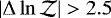 ). The reason for this is probably the low activity amplitude of ~ 3 m s−1 combined with the fact that only roughly three periods were covered by the RV observations (~ 350-day baseline compared to a period of ~120 d). Nonetheless, considering that even small influences from stellar activity can affect the planetary parameters (e.g. Stock et al. 2020a), and that even strong activity signals do not have to be evident in the periodogram (Nava et al. 2020), we proceeded with the models that include the GP.
Of these models, those that consider eccentric orbits for one of the two signals are at best indistinguishable  ) from the model with the highest log evidence, which considers only circular orbits. It can therefore be assumed that the two signals have a low eccentricity, if any. For such low-eccentricity orbits, however, the value is mainly determined by the large error bars and the phase coverage of our RV measurements (Hara et al. 2019). This ambiguity isreflected in the indistinguishability of the models and the unconstrained posteriors of the eccentricities (e2.6 d = 0.28 ± 0.23; e14.3 d = 0.20 ± 0.20). For the transiting planet, also considering its short period, it is therefore justified to assume a circular orbit in our further modelling (van Eylen et al. 2019). Since we do not know the nature of the 14.3-day signal, we proceeded with it in the same way in order to be consistent, and chose the model considering two circular signals for the joint fit.
To exclude the possibility that the choice of our model significantly influences the parameters of the transit planet candidate, we compared the fitted semi-amplitudes and the resulting minimum masses for the different models (Fig. B.2). Additionally, we performed a fit corresponding to the 2P(2.6 d,14.3 d) + dSHO-GP(120 d) model, but replacing the period prior of the 14.3-day signal with a prior considering the 15.0-day alias. All models agree within the interquartile range and show no significant differences. Yet, choosing the 15.0-day alias instead of the 14.3-day period results in a slightly higher planet mass, as is the case for most of the other models. However, those higher masses are also generally accompanied by larger errors.
4.6 Joint modelling
The highest information content is provided by the combination of the transit and RV data, which is why we performed a joint fit to derive precise parameters of the transiting planet. Based on our results from the transit- and RV-only analyses, the model consists of a circular orbit for the transiting planet with P ≈ 2.62 d fitted to the transit and RV data, in combination with the sinusoidal 14.3-day signal, and the dSHO-GP representing the stellar activity, in the RV data only. The priors used for the fit correspond to the combination of the transit- and RV-only priors as described inSects. 4.4 and 4.5 and are summarised in Table C.1.
We present the posterior parameters of the transiting planet, the 14.3-day signal, and the GP in Table 4, while the posteriors of the instrumental parameters are shown in Table D.1. Plots of the final models retrieved from the posteriors are shown in Fig. 6 for the RVs and Fig. 7 for the transits.
Given the uncertainty of 35% in the RV semi-amplitude of the transiting planet candidate, we checked whether our choice of the 14.3-day signal as the period underlying the ~15-day aliases had a significant effect on the planetary parameters. In Appendix E the results from a joint fit considering the 15.0-dayperiod to be the true period are presented. While the derived RV semi-amplitude for the transiting planet candidate isindeed slightly larger, it is fully consistent with the results presented here. Coincidentally, the higher amplitude in combination with the approximately unchanged uncertainties resulted in a significant measurement (~ 3.4σ). However, following the analysis in Sect. 4.5.2 and Appendix A, we were confident that P ≈ 14.3 d is the true period and, therefore, we accepted the non-significant amplitude from the corresponding fit.
Median posterior parameters of the transiting planet, the ~14.3 d signal, and the GP.
4.7 Stellar rotation period
4.7.1 Activity indicators
The wide wavelength range of CARMENES allows us to compute many indicators that are sensitive to stellar activity. A full list of all activity indicators that are routinely derived from the CARMENES spectra can be found in Zechmeister et al. (2018, spectral indices), Schöfer et al. (2019, photospheric and chromospheric indices), and Lafarga et al. (2020, parameters related to the cross-correlation function). For the sake of clarity, we only selected the indicators from the VIS channel that exhibit signals with FAP < 1% in a GLS periodogram and present them in Fig. 8. None of these signals coincide with the period of the transiting planet candidate or the 14.3-day signal. However, all periodograms show a fairly similar pattern of peaks between 50 d to 300 d. The cause here is also a strong aliasing due to the seasonal observability of GJ 3929 and the resulting strong sampling frequency of fs ≈ 1∕292 d−1 (see also Sect. 4.5).
Particularly prominent is the Hα index derived from serval, which shows the strongest peak at a period of ~ 118 d, in combination with its first-order aliases at ~82 d and ~ 212 d. Additionally, there is another significant peak of ~65 days, which could be misinterpreted as the second harmonic (≡P∕2) of the 118-day period, but it is actually closer to its second-order alias. The oppositely signed counterpart of this second order alias produces a significant long-term trend in the data. This is similar to the periodogram of the chromatic index (CRX; Zechmeister et al. 2018), which is consistent with either an underlying period of ~ 128 d that shows aliasing up to third order, or a ~70-day periodicity producing up to second-order aliases. Furthermore, analogous patterns can be found for the Ca II infrared triple b (IRT b) index as well as the TiO λ8430 Å band. The Na I D doublet lines and the other two TiO bands are dominated by long-term trends. However, they can also be explained by aliasing of underlying periods of about 113 d (see Appendix F for a detailed list of the peaks and corresponding aliases).
 |
Fig. 6 Results for the CARMENES RV from the joint fit with the transits. The black lines show the median of 10 000 samples from the posterior and the blue shaded areas denote the 68%, 95%, and 99% credibility intervals, respectively. The orange line shows the GP model. Error bars of the measurements include the instrumental jitter added in quadrature. The residuals after subtracting the median models are shown in the lower panels of each plot. Top: RVs over time. Bottom: RVs phase-folded to the periods of the transiting planet (left) and the 14.3 d signal (right). |
4.7.2 Long-term photometry
We created GLS periodograms of the HATNet, ASAS-SN, and TJO data (see the first three panels of Fig. 8). The GLS of the HATNet data shows a highly significant peak at a period of P ≈ 57 d, which is consistent with the rotation period reported by Hartman et al. (2011), who applied a variance period-finder using a harmonic series. However, the detection of the period was flagged as ‘questionable’ by the authors following their visual inspection of the light curve as they did not recognise a clear variability by eye. The ASAS-SN data, on the other hand, show two prominent peaks in the GLS: one at P ≈ 91 d and an even more significant one at P ≈ 122 d. A look at the window function of the data shows that these two peaks are generated by aliasing due to a sampling frequency of fs ≈ 1∕362 d−1. The 122 d period is also supported by the TJO data. They show a peak at about 140 d, which is, due to the short baseline, embedded in a plateau for periods larger than 100 d.
The photometry and spectroscopic activity indicators thus share a common periodicity of about ~ 120 d, which is about twice the period published by Hartman et al. (2011) based on the HATNet data alone. However, it is reasonable that P ≈ 120 d is the actual rotation period of the star and that HATNet shows the second harmonic.
We therefore moved forward and performed a combined fit of the HATNet, ASAS-SN, and TJO data using the dSHO-GP model as in Kossakowski et al. (2021) to determine a precise value for it. In doing so, we used normally distributed priors for the instrumental offsets centred around 0 with a standard deviation of 0.1 and log-uniform priors for the instrumental jitter terms between 1 ppm to 10 × 106 ppm. For the GP hyperparameters, we used separate instrument priors for the standard deviation, σGP,phot (log-uniform between 1 × 10⁻⁸ and 1), the quality factor of the secondary oscillation Q0 and the difference compared to the quality factor of the primary oscillation dQGP,phot (both log uniform between 0.1 and 1 × 10⁴), and the fractional amplitude, fGP,phot between both (uniform between 0 and 1). The GP rotation period of PGP,phot, however, was shared between all instruments with a uniform prior between 100 d to 150 d to avoid the 91-day alias of the ASAS-SN data and the 57-day second-order harmonic of the HATNet data. In this way, we determined a photometric rotation period of Prot = 122 ± 13 d.
We obtained three different measurements of the stellar rotation period: 126.5 ± 2.5 d from the RV measurements (Table 4), ~ 113–132 d from the activity indicators, and 122 ± 13 d from the photometry. All three measurements are consistent with each other. Causes for the differences in the measured periods can be different active latitudes at the times of the measurement, differential rotation, or, in the case of the activity indicators, the differences between photospheric and chromospheric indicators. Since photometrically determined rotation periods are often considered to be the most reliable and the RV measurement has a likely underestimated uncertainty, as the rotation period of GJ 3929 we adopt the photometric period of Prot = 122 ± 13 d, which, fittingly, comprises all three measurements the best.
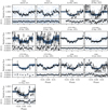 |
Fig. 7 Results from the joint fit for the transit observations. The black lines represent the median of 10 000 samples from the posterior phase-folded to the period of the transiting planet. Credibility intervals of 68%, 95%, and 99% are displayed by the blue shaded areas. The black points show the data binned to 0.001 in phase, and the measurements that were used for the fit are denoted by the blue dots. As for the RVs, the residuals after subtracting the median model are shown in the lower panel of each plot. |
5 Discussion
5.1 GJ 3929 b
Our analysis confirms the planetary nature of the transiting planet GJ 3929 b. Table 5 shows the planetary parameters derived from our joint fit. Its mass and radius of Mb = 1.21 ± 0.42 M⊕ and Rb = 1.150 ± 0.040 R⊕, respectively, put it into the regime of small Earth-sized planets. This makes GJ 3929 b comparable to other planets with confirmed masses orbiting M stars that were detected by TESS. These include, for example (in order of their detection), L 98-59 b (Kostov et al. 2019; Cloutier et al. 2019; Demangeon et al. 2021), TOI-270 b (Günther et al. 2019; van Eylen et al. 2021), GJ 357 b (Luque et al. 2019; Jenkins et al. 2019), GJ 1252 b (Shporer et al. 2020), GJ 3473 b (Kemmer et al. 2020), LHS-1140 c (Ment et al. 2019; Lillo-Box et al. 2020), and LHS 1478 b (Soto et al. 2021).
Although the uncertainty in mass allows a wide range of compositions for GJ 3929 b (see Fig. 9), its small radius places it below the radius gap for M-dwarf planets (Cloutier & Menou 2020; van Eylen et al. 2021) and, hence, makes a rocky composition very likely. The derived mean density of ρb = 4.4 ± 1.6 g cm−3 is compatible with an MgSiO3-dominated composition. GJ 3929 b thus expands the statistical sample of rocky super-Earths needed to further investigate the properties of the radius gap. For example, as a planet orbiting a mid-type M star, it is an important contribution for studies considering the dependence of the gap on the stellar mass or the incident flux, as in van Eylen et al. (2021).
With anorbital period of Pb = 2.62 d, GJ 3929 b receives 17.5 ± 1.3 times the solar flux on Earth, which corresponds to an equilibrium temperature of Teq= 568.8 ± 9.4 K (assuming zero Bond albedo). In combination with the host star brightness (J = 8.694 mag), this results in a transmission spectroscopy metric (TSM; Kempton et al. 2018) of 25.0± 13.2. GJ 3929 b is thus above the threshold of TSM > 10 determined by Kempton et al. (2018) and slightly larger than GJ 357 b (TSM = 23.4; Luque et al. 2019), which is considered one of the prime targets for atmospheric follow-up observations of rocky exoplanets with the upcoming JWST (Gardner et al. 2006).
Although unlikely given the Earth-like radius and consequently location below the radius gap, the uncertainty in the determined density does not completely exclude the presence of a significant atmosphere. An atmosphere with a high mean molecular weight would be difficult to probe, however, as it has been shown for other comparable small M-dwarf planets (e.g. Luque et al. 2019; Bower et al. 2019; Nowak et al. 2020), the dominant species of carbon dioxide and water are expected to produce absorption features that are observable with instruments such as the JWST or the ELT (Gilmozzi & Spyromilio 2007). The systematic in-depth atmospheric characterisation of rocky planets such as GJ 3929 b is expected to provide answers to questions regarding the abundance and composition of retained primordial atmospheres or secondary atmospheres formed by outgassing.
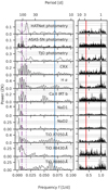 |
Fig. 8 GLS periodograms of photometry and activity indicators. The first three panels show the photometry from HATNet, ASAS-SN, and TJO, and the following panels show the activity indicators derived from CARMENES, which show signals with less than 1% FAP. The stellar rotation of P ≈ 122 d, as determined from the photometry, is indicated by the purple dot-dashed line and its second harmonic (P∕2) by the purple dotted line. As in Fig. 4, the period of the transiting planet is denoted by the red solid line, and the ~15 d periodicity is marked in blue, respectively. We normalised the power using the parameterisation of Zechmeister & Kürster (2009) and the 10, 1, and 0.1% false alarm probabilities denoted by the horizontal grey dashed lines are calculated using the analytic expression. |
Derived planet parameters for GJ 3929 b and the planet candidate.
5.2 Planet candidate GJ 3929 [c]
The strongest signal in the CARMENES RV data is not related to the transiting planet or the stellar rotation. It has a period of P[c] = 14.303 ± 0.035 d and an RV semi-amplitude of K[c] = 3.04 ± 0.44 m s−1. A stability analysis of the signal using tools such as the stacked Bayesian GLS (Mortier et al. 2015) is not meaningful because the seasonal observability leads to strong aliasing after the first block of observations and thus a strong loss in signal strength due to the splitting peaks. In combination with the FAP of the signal, which is still higher than 0.1% in the non-pre-whitened periodogram, we thus introduce it as a planet candidate, namely GJ 3929 [c]. The mass derived from the joint fit for this potential planet is M[c ] ≥ 5.27 ± 0.74 M⊕, which puts it into the regime of the sub-Neptune-mass planets.
In a co-planar orbit, such a planet could be transiting, even if only for a very small range (b[c] = 0.33 ± 0.23 assuming the inclination of the inner planet). Full transits should show signals comparable to or larger than those of the less massive inner planet. The fact that we do not detect any other potentially transiting signals in the TESS data after subtracting the 2.62-day planet suggests that there could be shallow grazing transits, if any. However, confirming the detection of such transits would be complicated by the uncertainty of the ephemeris as determined from the RVs – ttransit, m = 2459072.44 ± 0.41 d + m * 14.303 ± 0.035 d – which makes it furthermore plausible that some transits could fall just inside the data gaps of TESS. This is important to note, because applying a TLS periodogram to the unbinned HATNet data in the range of 0 d to 40 d gives rise to a spurious signal with a signal detection efficiency of approximately 9.75 (i.e. FAP < 0.01%) at a period of P ≈ 14.14 d and with a transit depth of ≈2.2 ± 1.8 ppt (see Fig. B.3). Moreover, even though unexpected, the GLS of the unbinned HATNet data shows, besides the strongest peak at the stellar rotation period, a highly significant peak at P ≈ 14.5 d and another peak with FAP < 1% at P ≈ 2.63 d. Any attempt in fitting the transiting planet together with or without the planet candidate to the HATNet data, however, brought up questionableresults. Furthermore, subtracting the GP model from the determination of the stellar rotation makes the signal disappear. The proximity of the signal’s period to half of the Moon’s cycle in combination with the large scatter of the unbinned HATNet data (rms = 6.7 ppt) suggests a questionableorigin of the signal, though we cannot rule out a transit scenario. If the planet were indeed transiting, we would expect a transit depth of ~1 ppt to 8 ppt for it based on its minimum mass and the corresponding empirical radius distribution in Fig. 9.
5.3 Implications for a multi-planet system
Planets such as the candidate GJ 3929 [c] in combination with GJ 3929 b are frequently detected (e.g. Sabotta et al. 2021; Cloutier et al. 2021). Moreover, combinations of terrestrial planets and sub-Neptunes are also commonly predicted by population synthesis models based on the core accretion paradigm of planet formation (Emsenhuber et al. 2021; Schlecker et al. 2021; Burn et al. 2021). Following the angular momentum deficit stability criterium from Laskar & Petit (2017), the system would be stable for eccentricities of the outer companion candidate up to 0.45.
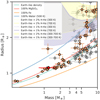 |
Fig. 9 Mass-radius diagram of well-characterised planets with R < 3 R⊕ and M < 10 M⊕. The plot shows the planets from the TEPcat catalogue (Southworth 2011, visited on 8 November 2021) with ΔM and ΔR < 30%. Planets withhost star temperatures Teff < 4000 K are shown in orange, and planets with hotter hosts are shown in grey. GJ 3929 b is marked with a red diamond. Additionally, theoretical mass-radius relations from Zeng et al. (2019) are shown for reference. |
6 Conclusions
The analysis of the TESS transit observations, in combination with the RV follow-up from CARMENES and transit follow-up from SAINT-EX and LCOGT, confirms the planetary nature of the Earth-sized, short-period planet, GJ 3929 b. Along with the brightness of its M-dwarf host, its high equilibrium temperature makes GJ 3929 b a prime target for atmospheric follow-up with the upcoming generation of facilities, such as the JWST, which will provide unique insight into the composition and, thus, formation and evolution of small and rocky planets.
Moreover, the RV measurements showed evidence for a second sub-Neptunian-mass planet candidate, namely GJ 3929 [c]. Its period is farfrom the rotation period of the star that we determined from archival photometry, and, therefore, it is not likely linked to stellar activity. Besides this, the candidate is promising because we detected a signal in the TLS periodogram of archival photometric HATNet data close to the orbital period determined from the RVs. Yet, additional follow-up is needed to confirm its planetary nature, given that the strong aliasing of the RVs and the time gap with respect to the HATNet data made it difficult to provide an in-depth investigation of the signal.
If the planetary nature of GJ 3929 [c] can indeed be proven, the GJ 3929 system would join the growing number of multi-planetary systems with relatively short periods around M-dwarf stars. Of particular interest would be whether GJ 3929 [c] is actually a transiting planet and, thus, whether it would be possible to determine its density.
Acknowledgements
CARMENES is an instrument for the Centro Astronómico Hispano-Alemán de Calar Alto (CAHA, Almerá, Spain). CARMENES is funded by the German Max-Planck-Gesellschaft (MPG), the Spanish Consejo Superior de Investigaciones Científicas (CSIC), the European Union through FEDER/ERF FICTS-2011-02 funds, and the members of the CARMENES Consortium (MaxPlanck-Institut für Astronomie, Instituto de Astrofísica de Andalucía, Landessternwarte Königstuhl, Institut de Ciències de l’Espai, Insitut für Astrophysik Göttingen, Universidad Complutense de Madrid, Thüringer Landessternwarte Tautenburg, Instituto de Astrofísica de Canarias, Hamburger Sternwarte, Centro de Astrobiología and Centro Astronómico HispanoAlemán), with additional contributions by the Spanish Ministry of Economy, the German Science Foundation through the Major Research Instrumentation Programme and DFG Research Unit FOR2544 “Blue Planets around Red Stars”, the Klaus Tschira Stiftung, the states of Baden-Württemberg and Niedersachsen, and by the Junta de Andalucía. Funding for the TESS mission is provided by NASA’s Science Mission directorate. We acknowledge the use of public TESS Alert data from pipelines at the TESS Science Office and at the TESS Science Processing Operations Center. This research has made use of the Exoplanet Follow-up Observation Program website, which is operated by the California Institute of Technology, under contract with the National Aeronautics and Space Administration under the Exoplanet Exploration Program. Resources supporting this work were provided by the NASA High-End Computing Program through the NASA Advanced Supercomputing Division at Ames Research Center for the production of the SPOC data products. This paper includes data collected by the TESS mission, which are publicly available from the Mikulski Archive for Space Telescopes. This work makes use of observations from the LCOGT network. Part of the LCOGT telescope time was granted by NOIRLab through the Mid-Scale Innovations Program (MSIP). MSIP is funded by NSF. This paper is based on observations made with the MuSCAT3 instrument, developed by the Astrobiology Center and under financial supports by JSPS KAKENHI (JP18H05439) and JST PRESTO (JPMJPR1775), at Faulkes Telescope North on Maui, HI, operated by the Las Cumbres Observatory. This work includes observationscarried out at the Observatorio Astronómico Nacional on the Sierra de San Pedro Mártir (OAN-SPM), Baja California, México. We acknowledge financial support from the Agencia Estatal de Investigación of the Ministerio de Ciencia, Innovación y Universidades and the ERDF through projects PID2019-109522GB-C5[1:4], PID2019-107061GB-C64, PID2019-110689RB-100, ESP2017-87676-C5-1-R, and the Centre of Excellence “Severo Ochoa” and “María de Maeztu” awards to the Instituto de Astrofísica de Canarias (CEX2019-000920-S), Instituto de Astrofísica de Andalucía (SEV-2017-0709), and Centro de Astrobiología (MDM-2017-0737), the Swiss National Science Foundation (PP00P2-163967 and PP00P2-190080), the Centre for Space and Habitability of the University of Bern, the National Centre for Competence in Research PlanetS, supported by the Swiss National Science Foundation, the Deutsche Forschungsgemeinschaft priority program SPP 1992 “Exploring the Diversity of Extrasolar Planets” (JE 701/5-1), the Excellence Cluster ORIGINS, which is funded by the Deutsche Forschungsgemeinschaft under Germany’s Excellence Strategy (EXC-2094 – 390783311), NASA (NNX17AG24G), JSPS KAKENHI Grant Number JP18H05439, JST CREST Grant Number JPMJCR1761, the Astrobiology Center of National Institutes of Natural Sciences (NINS) (Grant Number AB031010), the UNAM-DGAPA PAPIIT (BG-101321), the “la Caixa” Foundation (100010434), the European Union Horizon 2020 research and innovation programme under the Marie Skłodowska-Curie (No. 847648, fellowship code LCF/BQ/PI20/11760023), and the Generalitat de Catalunya/CERCA programme. Data were partly collected with the 90-cm telescope at Observatorio de Sierra Nevada (OSN), operated by the Instituto de Astrofísica de Andalucí a (IAA, CSIC). We deeply acknowledge the OSN telescope operators for their very appreciable support. The analysis of this work has made use of a wide variety of public available software packages that are not referenced in the manuscript: AstroImageJ (Collins et al. 2017), astropy Astropy Collaboration (2018), scipy (Virtanen et al. 2020), numpy (Oliphant 2006), matplotlib (Hunter 2007), tqdm (da Costa-Luis 2019), pandas (The pandas development team 2020), seaborn (Waskom et al. 2020), lightkurve (Lightkurve Collaboration 2018), radvel (Fulton et al. 2018), batman (Kreidberg 2015), dynesty (Speagle 2020), george (Ambikasaran et al. 2015), celerite (Foreman-Mackey et al. 2017), PyFITS (Barrett et al. 2012), astrobase Waqas Bhatti et al. (2020), scikit-learn (Pedregosa et al. 2011), TAPIR (Jensen 2013), Astrometry.net (Lang et al. 2010), photutils (Bradley et al. 2021), lmfit (Newville et al. 2021), tpfplotter (www.github.com/jlillo/tpfplotter).
Appendix A Differentiating aliases using posterior samples
The AliasFinder is based on creating synthetic data from the periods, amplitudes, and phases retrieved from an observed periodogram (Stock & Kemmer 2020; Stock et al. 2020a). One advantage of this approach is that it allows us to perform an alias analysis solely from a given set of RV measurements. However, in the presence of additional signals unrelated to the aliases in question (e.g. additional planets or stellar activity), those have to be taken into account by pre-whitening the data to mitigate their influence on the observed periodogram and make it comparable to the synthetic data. Yet, stellar activity, which often produces only quasi-periodic signals, poses a problem in this respect: the GPs that are commonly used to model such signals are not static model components, but they parametrise the covariance between the data points. This makes the pre-whitening impossible, because if the signal in question is omitted during pre-whitening, the GP model will be influenced by it and may absorb it from the residuals. Conversely, if the signal in question is taken into account in the pre-whitening (and later reinserted into the data), the GP model implies its presence in the residuals. In both cases, the signals recovered from the residual data do not resemble those of the original data and thus defeat the object of AliasFinder.
Bayesian modelling approaches, such as the nested sampling used in our analysis, however, offer a direct solution to this issue: the results from the posterior can also be adopted to generate the synthetic RV models used to create the comparison periodograms. In this way each model can include all required components of the fit and thus make the resulting periodograms directly comparable with the observed periodogram. Pre-whitening is no longer necessary in this case.
The procedure is as follows: For each possible alias period that is going to be investigated, a fit has to be performed. Thereby, the period of the fitted alias signal needs to be reasonably constrained, such that other aliases are excluded. Furthermore, the fit should consider all other signals of interest. Then, the synthetic RVs can be created using the solutions from the individual posterior samples of the fit results. For each sample that is drawn, the RV model is calculated on the time stamps of the observations and the uncertainties of the original measurements are adopted — analogously to the method of the AliasFinder and Dawson & Fabrycky (2010). These model RVs, however, do not include any noise and would therefore result in highly significant peaks in the periodogram for each considered period. A good measure of the noise is the rms of the residuals after subtracting it from the observed data. As an analogy to the jitter determination in the AliasFinder, one can therefore add white noise to the synthetic models that are drawn from a normal distribution and follow the residual rms. The evaluation is then analogous to the AliasFinder. After calculating the GLS periodogram for all synthetic RV datasets, the median GLS and its confidence intervals, as well as the phases of the peaks, can be determined and compared to the observed GLS and its phases.
In Fig. A.1, we present the results from the 2P + dSHO − GP120d models as described in Sect. 4.5, where the second period was either constrained to the 14.3-day or 15.0-day period. The resulting synthetic periodograms are consistent with the results using the AliasFinder and also confirm that considering the 14.3-day period results in a better match to the observed periodogram.
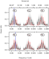 |
Fig. A.1 Alias test for the ~ 15 d and ~ 14.3 d periods using the posterior samples from the RV-only fits. We took 5000 posterior samples of the second component from the 2P + dSHO − GP120d models to produce synthetic periodograms (black lines), which can be compared with the periodogram of the observed data (red lines). The results for the model considering an ~ 15 d signal are shown in the first row, and the results for the ~ 14.3 d signal are in the second row, with each period indicated by a vertical blue dashed line, respectively. Black lines depict the median of the samples for each simulation, and the grey shaded areas are the 50, 90, and 99% confidence intervals. Furthermore, the phases of the peaks as measured from the GLS are displayed in the circles, following the same colour scheme (the grey shades denote the standard deviations of the simulated peaks). |
Appendix B Additional figures and tables
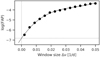 |
Fig. B.1 Determining the FAP for the signal of the transiting planet in the RVs. For each window size, the FAP was calculated comparing the combined power of the highest peaks appearing around the 2.62-day period of the transiting planet candidate and the 1.62-day alias from 50 000 permutations with the combined power of the signals in the original GLS. The black line shows a third-order polynomial fit to the data, which is extrapolated to zero to determine the FAP. |
 |
Fig. B.2 Comparison of the amplitudes and resulting minimum masses for the different models considered. The box plots show the posterior distribution from the model comparison presented in the RV-only analysis (Sect. 4.5). The width of each box corresponds to the interquartile range (IQR), and the whiskers mark the first quartile minus 1.5× the IQR and the third quartile plus 1.5× the IQR, respectively. To facilitate the comparison, the grey dashed line shows the median posterior value of our selected model. |
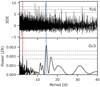 |
Fig. B.3 TLS and GLS periodgrams of the unbinned HATNet data. The periods of GJ 3929 b and the candidate GJ 3929 [c]are marked by the vertical red and blue lines, respectively. |
Photometry of GJ 3929.
Appendix C Priors for juliet
Priors used for juliet in the joint fit of transits and RV.
Appendix D Instrumental posteriors of the joint fit
Posteriors of the joint fit for the different instrumental parameters.
Appendix E Alternative joint fit considering P2 ~ 15 d
In this section, we present an alternative joint fit, in which we consider the 15.0 d period to be the signal underlying the aliases discussed in Sect. 4.5.2. The priors are identical to the joint fit in Sect. 4.6, except the prior for the period of the second component, which was set uniform between 14.71 d to 15.48 d according to its peak width in the GLS periodogram. The posterior for the transiting planet, the 15.0 d signal and the GP for this fit are shown in Table E.1, and the resulting planetary parameters for GJ 3929 b are in Table E.2. We found no significant deviation and almost identical uncertainties for the transiting planet compared to the values obtained from considering the 14.3-day period. However, the mass of the 15.0-day candidate is noticeably smaller and more uncertain compared to the fit considering the 14.3-day period. Nevertheless, the higher planetary mass of GJ 3929 b derived from the 15.0-day fit, which was already evident in the RV-only fit, in combination with the consistent uncertainties, leads to a significant (> 3σ) mass measurement.
Median posterior parameters from the alternative joint fit for the transiting planet, the ~ 15.0 d signal, and the GP.
Alternative derived planet parameters for GJ 3929 b and the planet candidate considering the 15.0 d period.
Appendix F Detailed record of the peaks and aliases visible in the GLS periodograms of the activity indicators
Peaks of interest and their appearing aliases in the activity indicator periodograms.
References
- Ahn, C. P., Alexandroff, R., Allende Prieto, C., et al. 2012, ApJS, 203, 21 [Google Scholar]
- Aller, A., Lillo-Box, J., Jones, D., Miranda, L. F., & Barceló Forteza, S. 2020, A&A, 635, A128 [NASA ADS] [CrossRef] [EDP Sciences] [Google Scholar]
- Amado, P. J., Bauer, F. F., RodrRodrCardona Guillén, C., et al. 2021, A&A, 650, A188 [NASA ADS] [CrossRef] [EDP Sciences] [Google Scholar]
- Ambikasaran, S., Foreman-Mackey, D., Greengard, L., Hogg, D. W., & O’Neil, M. 2015, IEEE Trans. Pattern Anal. Mach. Intell., 38, 252 [Google Scholar]
- Astropy Collaboration (Price-Whelan, A. M., et al.) 2018, AJ, 156, 123 [Google Scholar]
- Astudillo-Defru, N., Cloutier, R., Wang, S. X., et al. 2020, A&A, 636, A58 [NASA ADS] [CrossRef] [EDP Sciences] [Google Scholar]
- Bakos, G., Noyes, R. W., Kovács, G., et al. 2004, PASP, 116, 266 [NASA ADS] [CrossRef] [Google Scholar]
- Bakos, G., Noyes, R. W., Latham, D. W., et al. 2006, in Tenth Anniversary of 51 Peg-b: Status of and prospects for hot Jupiter studies, eds. L. Arnold, F. Bouchy, & C. Moutou, 184 [Google Scholar]
- Barnes, J. W. 2007, PASP, 119, 986 [NASA ADS] [CrossRef] [Google Scholar]
- Barrett, P., Hsu, J. C., Hanley, C., et al. 2012, PyFITS: Python FITS Module [Google Scholar]
- Barstow, J. K., & Irwin, P. G. J. 2016, MNRAS, 461, L92 [NASA ADS] [CrossRef] [Google Scholar]
- Bauer, F. F., Zechmeister, M., Kaminski, A., et al. 2020, A&A, 640, A50 [NASA ADS] [CrossRef] [EDP Sciences] [Google Scholar]
- Bean, J. L., Raymond, S. N., & Owen, J. E. 2021, J. Geophys. Res. (Planets), 126, e06639 [NASA ADS] [Google Scholar]
- Bhatti, W., Bouma, L., Joshua, J., & Price-Whelan, A. 2020, https://doi.org/10.5281/zenodo.3723832 [Google Scholar]
- Bitsch, B., Raymond, S. N., & Izidoro, A. 2019, A&A, 624, A109 [NASA ADS] [CrossRef] [EDP Sciences] [Google Scholar]
- Bluhm, P., Luque, R., Espinoza, N., et al. 2020, A&A, 639, A132 [NASA ADS] [CrossRef] [EDP Sciences] [Google Scholar]
- Bluhm, P., Pallé, E., Molaverdikhani, K., et al. 2021, A&A, 650, A78 [NASA ADS] [CrossRef] [EDP Sciences] [Google Scholar]
- Bower, D. J., Kitzmann, D., Wolf, A. S., et al. 2019, A&A, 631, A103 [NASA ADS] [CrossRef] [EDP Sciences] [Google Scholar]
- Bradley, L., Sipocz, B., Robitaille, T., et al. 2021, https://doi.org/10.5281/zenodo.4453725 [Google Scholar]
- Brown, T. M., Baliber, N., Bianco, F. B., et al. 2013, PASP, 125, 1031 [Google Scholar]
- Burn, R., Schlecker, M., Mordasini, C., et al. 2021, A&A, 656, A72 [NASA ADS] [CrossRef] [EDP Sciences] [Google Scholar]
- Caballero, J. A., Cortés-Contreras, M., Alonso-Floriano, F. J., et al. 2016a, in 19th Cambridge Workshop on Cool Stars, Stellar Systems and the Sun, 148 [Google Scholar]
- Caballero, J. A., Guàrdia, J., López del Fresno, M., et al. 2016b, in Proc. SPIE, 9910, Observatory Operations: Strategies, Processes, and Systems VI, 99100E [Google Scholar]
- Cifuentes, C., Caballero, J. A., Cortés-Contreras, M., et al. 2020, A&A, 642, A115 [NASA ADS] [CrossRef] [EDP Sciences] [Google Scholar]
- Cloutier, R., & Menou, K. 2020, AJ, 159, 211 [NASA ADS] [CrossRef] [Google Scholar]
- Cloutier, R., Astudillo-Defru, N., Bonfils, X., et al. 2019, A&A, 629, A111 [NASA ADS] [CrossRef] [EDP Sciences] [Google Scholar]
- Cloutier, R., Charbonneau, D., Deming, D., Bonfils, X., & Astudillo-Defru, N. 2021, AJ, 162, 174 [NASA ADS] [CrossRef] [Google Scholar]
- Collins, K. A., Kielkopf, J. F., Stassun, K. G., & Hessman, F. V. 2017, AJ, 153, 77 [Google Scholar]
- Colome, J., & Ribas, I. 2006, IAU Special Session, 6, 11 [Google Scholar]
- Colomé, J., Casteels, K., Ribas, I., & Francisco, X. 2010, SPIE Conf. Ser., 7740, 77403K [Google Scholar]
- Cortés-Contreras, M. 2017, PhD thesis, Universidad Complutense de Madrid [Google Scholar]
- Cutri, R. M. & et al. 2012, VizieR Online Data Catalog: II/311 [Google Scholar]
- da Costa-Luis, C. 2019, J. Open Source Softw., 4, 1277 [NASA ADS] [CrossRef] [Google Scholar]
- Dai, F., Masuda, K., Winn, J. N., & Zeng, L. 2019, ApJ, 883, 79 [NASA ADS] [CrossRef] [Google Scholar]
- Dawson, R. I., & Fabrycky, D. C. 2010, ApJ, 722, 937 [Google Scholar]
- Demangeon, O. D. S., Zapatero Osorio, M. R., Alibert, Y., et al. 2021, A&A, 653, A41 [NASA ADS] [CrossRef] [EDP Sciences] [Google Scholar]
- Demory, B.-O., Pozuelos, F. J., Gómez Maqueo Chew, Y., et al. 2020, A&A, 642, A49 [NASA ADS] [CrossRef] [EDP Sciences] [Google Scholar]
- Dreizler, S., Crossfield, I. J. M., Kossakowski, D., & et al. 2021, A&A, 644, A127 [Google Scholar]
- Emsenhuber, A., Mordasini, C., Burn, R., et al. 2021, A&A, 656, A69 [NASA ADS] [CrossRef] [EDP Sciences] [Google Scholar]
- Espinoza, N. 2018, RNAAS, 2, 209 [Google Scholar]
- Espinoza, N., & Jordán, A. 2015, MNRAS, 450, 1879 [Google Scholar]
- Espinoza, N., Kossakowski, D., & Brahm, R. 2019, MNRAS, 490, 2262 [Google Scholar]
- Foreman-Mackey, D., Agol, E., Angus, R., & Ambikasaran, S. 2017, AJ, 154, 220 [NASA ADS] [CrossRef] [Google Scholar]
- Fulton, B. J., Petigura, E. A., Howard, A. W., et al. 2017, AJ, 154, 109 [Google Scholar]
- Fulton, B. J., Petigura, E. A., Blunt, S., & Sinukoff, E. 2018, PASP, 130, 044504 [Google Scholar]
- Gaia Collaboration (Brown, A. G. A., et al.) 2018, A&A, 616, A1 [NASA ADS] [CrossRef] [EDP Sciences] [Google Scholar]
- Gaia Collaboration (Brown, A. G. A., et al.) 2021, A&A, 649, A1 [NASA ADS] [CrossRef] [EDP Sciences] [Google Scholar]
- Gardner, J. P., Mather, J. C., Clampin, M., et al. 2006, Space Sci. Rev., 123, 485 [Google Scholar]
- Giclas, H. L., Slaughter, C. D., & Burnham, R. 1959, Lowell Observ. Bull., 4, 136 [Google Scholar]
- Gilmozzi, R., & Spyromilio, J. 2007, The Messenger, 127, 11 [Google Scholar]
- Ginzburg, S., Schlichting, H. E., & Sari, R. 2018, MNRAS, 476, 759 [Google Scholar]
- Girardi, L., Barbieri, M., Groenewegen, M. A. T., et al. 2012, Astrophys. Space Sci. Proc., 26, 165 [Google Scholar]
- Gliese, W., & Jahreiß, H. 1991, Preliminary Version of the Third Catalogue of Nearby Stars, eds. L.E. Brotzmann, & S.E. Gesser [Google Scholar]
- Guerrero, N. M., Seager, S., Huang, C. X., et al. 2021, ApJS, 254, 39 [NASA ADS] [CrossRef] [Google Scholar]
- Gupta, A., & Schlichting, H. E. 2019, MNRAS, 487, 24 [Google Scholar]
- Günther, M. N., Pozuelos, F. J., Dittmann, J. A., et al. 2019, Nat. Astron., 3, 1099 [Google Scholar]
- Hara, N. C., Boué, G., Laskar, J., Delisle, J.-B., & Unger, N. 2019, MNRAS, 489, 738 [NASA ADS] [CrossRef] [Google Scholar]
- Hartman, J. D., Bakos, G. A., Noyes, R. W., et al. 2011, AJ, 141, 166 [NASA ADS] [CrossRef] [Google Scholar]
- Hatzes, A. P. 2019, The Doppler Method for the Detection of Exoplanets (Bristol, UK: IOP Publishing) [Google Scholar]
- Hippke, M., & Heller, R. 2019, A&A, 623, A39 [NASA ADS] [CrossRef] [EDP Sciences] [Google Scholar]
- Hormuth, F., Brandner, W., Hippler, S., & Henning, T. 2008, J. Phys. Conf. Ser., 131, 012051 [Google Scholar]
- Hunter, J. D. 2007, Comput. Sci. Eng., 9, 90 [NASA ADS] [CrossRef] [Google Scholar]
- Jeffers, S. V., Schöfer, P., Lamert, A., et al. 2018, A&A, 614, A76 [NASA ADS] [CrossRef] [EDP Sciences] [Google Scholar]
- Jeffers, S. V., Dreizler, S., Barnes, J. R., et al. 2020, Science, 368, 1477 [Google Scholar]
- Jenkins, J. M., Caldwell, D. A., & Borucki, W. J. 2002, ApJ, 564, 495 [NASA ADS] [CrossRef] [Google Scholar]
- Jenkins, J. M., Chandrasekaran, H., McCauliff, S. D., et al. 2010, SPIE Conf. Ser., 7740, 77400D [Google Scholar]
- Jenkins, J. M., Twicken, J. D., McCauliff, S., et al. 2016, in SPIE Conf. Ser., 9913, 99133E [Google Scholar]
- Jenkins, J. S., Pozuelos, F. J., Tuomi, M., et al. 2019, MNRAS, 490, 5585 [Google Scholar]
- Jenkins, J. M., Tenenbaum, P., Seader, S., et al. 2020, Kepler Data Processing Handbook: Transiting Planet Search [Google Scholar]
- Jensen, E. 2013, Tapir: A web interface for transit/eclipse observability, Astrophysics Source Code Library [record ascl:1306.007] [Google Scholar]
- Jontof-Hutter, D. 2019, Ann. Rev. Earth Planet. Sci., 47, 141 [Google Scholar]
- Kemmer, J., Stock, S., Kossakowski, D., et al. 2020, A&A, 642, A236 [EDP Sciences] [Google Scholar]
- Kempton, E. M.-R., Bean, J. L., Louie, D. R., et al. 2018, PASP, 130, 114401 [CrossRef] [Google Scholar]
- Kipping, D. M. 2008, MNRAS, 389, 1383 [NASA ADS] [CrossRef] [Google Scholar]
- Kipping, D. M. 2013, A&A, 435, 2152 [Google Scholar]
- Kochanek, C. S., Shappee, B. J., Stanek, K. Z., et al. 2017, PASP, 129, 104502 [Google Scholar]
- Kossakowski, D., Kemmer, J., Bluhm, P., et al. 2021, A&A, 656, A124 [NASA ADS] [CrossRef] [EDP Sciences] [Google Scholar]
- Kostov, V. B., Schlieder, J. E., Barclay, T., et al. 2019, AJ, 158, 32 [Google Scholar]
- Kreidberg, L. 2015, PASP, 127, 1161 [Google Scholar]
- Lafarga, M., Ribas, I., Lovis, C., et al. 2020, A&A, 636, A36 [NASA ADS] [CrossRef] [EDP Sciences] [Google Scholar]
- Lang, D., Hogg, D. W., Mierle, K., Blanton, M., & Roweis, S. 2010, AJ, 139, 1782 [Google Scholar]
- Laskar, J., & Petit, A. C. 2017, A&A, 605, A72 [NASA ADS] [CrossRef] [EDP Sciences] [Google Scholar]
- Li, J., Tenenbaum, P., Twicken, J. D., et al. 2019, PASP, 131, 024506 [NASA ADS] [CrossRef] [Google Scholar]
- Lightkurve Collaboration (Cardoso, J. V. d. M., et al.) 2018, Lightkurve: Kepler and TESS time series analysis in Python, Astrophysics Source Code Library [record ascl:1812.013] [Google Scholar]
- Lillo-Box, J., Barrado, D., & Bouy, H. 2012, A&A, 546, A10 [NASA ADS] [CrossRef] [EDP Sciences] [Google Scholar]
- Lillo-Box, J., Barrado, D., & Bouy, H. 2014, A&A, 566, A103 [NASA ADS] [CrossRef] [EDP Sciences] [Google Scholar]
- Lillo-Box, J., Figueira, P., Leleu, A., et al. 2020, A&A, 642, A121 [NASA ADS] [CrossRef] [EDP Sciences] [Google Scholar]
- Lopez, E. D., & Fortney, J. J. 2014, ApJ, 792, 1 [Google Scholar]
- Luque, R., Pallé, E., Kossakowski, D., et al. 2019, A&A, 628, A39 [NASA ADS] [CrossRef] [EDP Sciences] [Google Scholar]
- Lépine, S., Hilton, E. J., Mann, A. W., et al. 2013, AJ, 145, 102 [Google Scholar]
- Marfil, E., Tabernero, H. M., Montes, D., et al. 2021, A&A, 656, A162 [NASA ADS] [CrossRef] [EDP Sciences] [Google Scholar]
- McCully, C., Turner, M., Volgenau, N., et al. 2018a, https://doi.org/10.5281/zenodo.1257560 [Google Scholar]
- McCully, C., Volgenau, N. H., Harbeck, D.-R., et al. 2018b, SPIE Conf. Ser., Proc. SPIE, 107070K [Google Scholar]
- Ment, K., Dittmann, J. A., Astudillo-Defru, N., et al. 2019, AJ, 157, 32 [NASA ADS] [CrossRef] [Google Scholar]
- Morley, C. V., Kreidberg, L., Rustamkulov, Z., Robinson, T., & Fortney, J. J. 2017, ApJ, 850, 121 [Google Scholar]
- Mortier, A., Faria, J. P., Correia, C. M., Santerne, A., & Santos, N. C. 2015, A&A, 573, A101 [NASA ADS] [CrossRef] [EDP Sciences] [Google Scholar]
- Narita, N., Fukui, A., Yamamuro, T., et al. 2020, SPIE Conf. Ser., 11447, 114475K [NASA ADS] [Google Scholar]
- Nava, C., López-Morales, M., Haywood, R. D., & Giles, H. A. C. 2020, AJ, 159, 23 [Google Scholar]
- Newville, M., Otten, R., Nelson, A., et al. 2021, https://doi.org/10.5281/zenodo.4516651 [Google Scholar]
- Nowak, G., Luque, R., Parviainen, H., et al. 2020, A&A, 642, A173 [NASA ADS] [CrossRef] [EDP Sciences] [Google Scholar]
- Oliphant, T. E. 2006, A guide to NumPy, 1 (Trelgol Publishing USA) [Google Scholar]
- Owen, J. E., & Wu, Y. 2013, ApJ, 775, 105 [Google Scholar]
- Owen, J. E., & Wu, Y. 2017, ApJ, 847, 29 [Google Scholar]
- Passegger, V. M., Schweitzer, A., Shulyak, D., et al. 2019, A&A, 627, A161 [NASA ADS] [CrossRef] [EDP Sciences] [Google Scholar]
- Pedregosa, F., Varoquaux, G., Gramfort, A., et al. 2011, J. Mach. Learn. Res., 12, 2825 [Google Scholar]
- Quirrenbach, A., Amado, P. J., Caballero, J. A., et al. 2014, in Proc. SPIE, 9147, Ground-based and Airborne Instrumentation for Astronomy V, 91471F [Google Scholar]
- Rauer, H., Gebauer, S., Paris, P. V., et al. 2011, A&A, 529, A8 [NASA ADS] [CrossRef] [EDP Sciences] [Google Scholar]
- Ricker, G. R., Winn, J. N., Vanderspek, R., et al. 2015, J. Astron. Telescopes Instrum. Syst., 1, 014003 [Google Scholar]
- Rogers, L. A. 2015, ApJ, 801, 41 [Google Scholar]
- Rogers, L. A.,& Seager, S. 2010, ApJ, 712, 974 [NASA ADS] [CrossRef] [Google Scholar]
- Sabotta, S., Schlecker, M., Chaturvedi, P., et al. 2021, A&A, 653, A114 [NASA ADS] [CrossRef] [EDP Sciences] [Google Scholar]
- Schlecker, M., Pham, D., Burn, R., et al. 2021, A&A, 656, A73 [NASA ADS] [CrossRef] [EDP Sciences] [Google Scholar]
- Schneider, A. C., Greco, J., Cushing, M. C., et al. 2016, ApJ, 817, 112 [Google Scholar]
- Schweitzer, A., Passegger, V. M., Cifuentes, C., et al. 2019, A&A, 625, A68 [NASA ADS] [CrossRef] [EDP Sciences] [Google Scholar]
- Schöfer, P., Jeffers, S. V., Reiners, A., et al. 2019, A&A, 623, A44 [Google Scholar]
- Shappee, B. J., Prieto, J. L., Grupe, D., et al. 2014, ApJ, 788, 48 [Google Scholar]
- Shporer, A., Collins, K. A., Astudillo-Defru, N., et al. 2020, ApJ, 890, L7 [Google Scholar]
- Skrutskie, M. F., Cutri, R. M., Stiening, R., et al. 2006, AJ, 131, 1163 [NASA ADS] [CrossRef] [Google Scholar]
- Smith, J. C., Stumpe, M. C., van Cleve, J. E., et al. 2012, PASP, 124, 1000 [NASA ADS] [CrossRef] [Google Scholar]
- Soto, M. G., Anglada-Escudé, G., Dreizler, S., et al. 2021, A&A, 649, A144 [NASA ADS] [CrossRef] [EDP Sciences] [Google Scholar]
- Southworth, J. 2011, MNRAS, 417, 2166 [Google Scholar]
- Speagle, J. S. 2020, MNRAS, 493, 3132 [Google Scholar]
- Stassun, K. G., Oelkers, R. J., Paegert, M., et al. 2019, AJ, 158, 138 [Google Scholar]
- Stefánsson, G., Kopparapu, R., Lin, A., et al. 2020, AJ, 160, 259 [CrossRef] [Google Scholar]
- Stock, S., & Kemmer, J. 2020, J. Open Source Softw., 5, 1771 [NASA ADS] [CrossRef] [Google Scholar]
- Stock, S., Kemmer, J., Reffert, S., et al. 2020a, A&A, 636, A119 [NASA ADS] [CrossRef] [EDP Sciences] [Google Scholar]
- Stock, S., Nagel, E., Kemmer, J., et al. 2020b, A&A, 643, A112 [EDP Sciences] [Google Scholar]
- Strehl, K. 1902, Astron. Nachr., 158, 89 [Google Scholar]
- Stumpe, M. C., Smith, J. C., van Cleve, J. E., et al. 2012, PASP, 124, 985 [NASA ADS] [CrossRef] [Google Scholar]
- Stumpe, M. C., Smith, J. C., Catanzarite, J. H., et al. 2014, PASP, 126, 100 [Google Scholar]
- The pandas development team, 2020, pandas-dev/pandas: Pandas [Google Scholar]
- Trifonov, T. 2019, The Exo-Striker: Transit and radial velocity interactive fitting tool for orbital analysis and N-body simulations, Astrophysics Source Code Library [record ascl:1906.004] [Google Scholar]
- Trifonov, T., Caballero, J. A., Morales, J. C., et al. 2021, Science, 371, 1038 [Google Scholar]
- Trotta, R. 2008, Contemp. Phys., 49, 71 [Google Scholar]
- Twicken, J. D., Catanzarite, J. H., Clarke, B. D., et al. 2018, PASP, 130, 064502 [Google Scholar]
- van Eylen, V., & Albrecht, S. 2015, ApJ, 808, 126 [NASA ADS] [CrossRef] [Google Scholar]
- van Eylen, V., Agentoft, C., Lundkvist, M. S., et al. 2018, MNRAS, 479, 4786 [NASA ADS] [CrossRef] [Google Scholar]
- van Eylen, V., Albrecht, S., Huang, X., et al. 2019, AJ, 157, 61 [NASA ADS] [CrossRef] [Google Scholar]
- van Eylen, V., Astudillo-Defru, N., Bonfils, X., et al. 2021, MNRAS, 507, 2154 [NASA ADS] [Google Scholar]
- Venturini, J., Guilera, O. M., Haldemann, J., & Ronco, MarMordasini, Christoph. 2020a, A&A, 643, L1 [NASA ADS] [CrossRef] [EDP Sciences] [Google Scholar]
- Venturini, J., Guilera, O. M., & Ronco, MarMordasini, Christoph. 2020b, A&A, 644, A174 [NASA ADS] [CrossRef] [EDP Sciences] [Google Scholar]
- Virtanen, P., Gommers, R., Oliphant Travis E., et al. 2020, Nat. Methods, 17, 261 [NASA ADS] [CrossRef] [Google Scholar]
- Waskom, M., Botvinnik, O., Ostblom, J., et al. 2020, https://doi.org/10.5281/zenodo.3767070 [Google Scholar]
- Wells, R. D., Rackham, B. V., Schanche, N., et al. 2021, A&A, 653, A97 [NASA ADS] [CrossRef] [EDP Sciences] [Google Scholar]
- Zacharias, N., Finch, C. T., Girard, T. M., et al. 2013, AJ, 145, 44 [Google Scholar]
- Zechmeister, M., & Kürster, M. 2009, A&A, 496, 577 [CrossRef] [EDP Sciences] [Google Scholar]
- Zechmeister, M., Reiners, A., Amado, P. J., et al. 2018, A&A, 609, A12 [NASA ADS] [CrossRef] [EDP Sciences] [Google Scholar]
- Zechmeister, M., Reiners, A., Amado, P. J., et al. 2020, SERVAL: SpEctrum Radial Velocity AnaLyser, Astrophysics Source Code Library [record ascl:2006.011] [Google Scholar]
- Zeng, L., Jacobsen, S. B., Sasselov, D. D., et al. 2019, Proc. Natl. Acad. Sci. U.S.A., 116, 9723 [Google Scholar]
Calar Alto high-Resolution search for M dwarfs with Exoearths with Near-infrared and visible Echelle Spectrographs, http://carmenes.caha.es
Searching and characterising transiting exoplanets.
Las Cumbres Observatory.
Multicolor Simultaneous Camera for studying Atmospheres of Transiting exoplanets 3.
These astrophysical stellar parameters agree within 1σ uncertainties with those recently published by Marfil et al. (2021).
All Tables
Median posterior parameters of the transiting planet, the ~14.3 d signal, and the GP.
Median posterior parameters from the alternative joint fit for the transiting planet, the ~ 15.0 d signal, and the GP.
Alternative derived planet parameters for GJ 3929 b and the planet candidate considering the 15.0 d period.
Peaks of interest and their appearing aliases in the activity indicator periodograms.
All Figures
|
Fig. 1 TESS PDCSAP light curves for sector 24 (top) and sector 25 (bottom). The blue points are the measurements and the black dots are 20 min bins. The transit times of GJ 3929 b are indicated by red ticks. |
| In the text | |
|
Fig. 2 TESS TPFs of GJ 3929. Top: TESS sector 24, bottom: TESS sector 25. The position of GJ 3929 is denoted by a white cross, and the aperture mask used to create the PDCSAP light curves is shown as the pixels with orange borders. For comparison, nearby sources from the Gaia DR2 catalogue (Gaia Collaboration 2018), up to a difference of Δm = 8 mag in brightness compared to GJ 3929, are plotted by red circles. Figure created using tpfplotter (Aller et al. 2020). |
| In the text | |
|
Fig. 3 Contrast curve of the AstraLux high-resolution image. The image used to create the contrast curve is shown in the inset. |
| In the text | |
|
Fig. 4 GLS periodogram analysis of the RVs. In the first panel, we show the window function of the CARMENES data. In the subsequent panels, the residuals after subtracting models of increasing complexity are presented. The components that were considered for the fits are listed in the inset texts (see also Table 3). The period, P = 2.62 d, and one-day alias, P = 1.62 d, of the transiting planet are marked by the red solid and dashed lines, while the ~ 15-day periodicity and its daily aliases are marked by blue solid and dashed lines, respectively. Additionally, even though insignificant in the periodogram, the stellar rotation period of P = 122 d (Sect. 4.7) is indicated by the purple dot-dashed line. We normalised the power using the parametrisation of Zechmeister & Kürster (2009), and the 10, 1, and 0.1% FAPs denoted by the horizontal grey dashed lines were calculated using the analytic expression. |
| In the text | |
|
Fig. 5 Alias test for the 14.3-day and 15.0-day periods using AliasFinder. We generated 5000 synthetic datasets for each period to produce synthetic periodograms (black lines), which are compared with the periodogram of the observed data (red lines). The simulation for the 15.0-day signal is shown in the top row and the simulation for the 14.3-day signal in the bottom row, each period indicated by a vertical blue dashed line, respectively. Black lines depict the median of the samples for each simulation, and the grey shaded areas are the 50, 90, and 99% confidence intervals. Furthermore, the phases of the peaks as determined by the GLS periodogram are displayed in the circles, following the same colour scheme (the grey shades denote the standard deviations of the simulated peaks). The black arrows point out the difference in the periodograms for the daily aliases that allows to identify the best matching period (see the text for the discussion). |
| In the text | |
|
Fig. 6 Results for the CARMENES RV from the joint fit with the transits. The black lines show the median of 10 000 samples from the posterior and the blue shaded areas denote the 68%, 95%, and 99% credibility intervals, respectively. The orange line shows the GP model. Error bars of the measurements include the instrumental jitter added in quadrature. The residuals after subtracting the median models are shown in the lower panels of each plot. Top: RVs over time. Bottom: RVs phase-folded to the periods of the transiting planet (left) and the 14.3 d signal (right). |
| In the text | |
|
Fig. 7 Results from the joint fit for the transit observations. The black lines represent the median of 10 000 samples from the posterior phase-folded to the period of the transiting planet. Credibility intervals of 68%, 95%, and 99% are displayed by the blue shaded areas. The black points show the data binned to 0.001 in phase, and the measurements that were used for the fit are denoted by the blue dots. As for the RVs, the residuals after subtracting the median model are shown in the lower panel of each plot. |
| In the text | |
|
Fig. 8 GLS periodograms of photometry and activity indicators. The first three panels show the photometry from HATNet, ASAS-SN, and TJO, and the following panels show the activity indicators derived from CARMENES, which show signals with less than 1% FAP. The stellar rotation of P ≈ 122 d, as determined from the photometry, is indicated by the purple dot-dashed line and its second harmonic (P∕2) by the purple dotted line. As in Fig. 4, the period of the transiting planet is denoted by the red solid line, and the ~15 d periodicity is marked in blue, respectively. We normalised the power using the parameterisation of Zechmeister & Kürster (2009) and the 10, 1, and 0.1% false alarm probabilities denoted by the horizontal grey dashed lines are calculated using the analytic expression. |
| In the text | |
|
Fig. 9 Mass-radius diagram of well-characterised planets with R < 3 R⊕ and M < 10 M⊕. The plot shows the planets from the TEPcat catalogue (Southworth 2011, visited on 8 November 2021) with ΔM and ΔR < 30%. Planets withhost star temperatures Teff < 4000 K are shown in orange, and planets with hotter hosts are shown in grey. GJ 3929 b is marked with a red diamond. Additionally, theoretical mass-radius relations from Zeng et al. (2019) are shown for reference. |
| In the text | |
|
Fig. A.1 Alias test for the ~ 15 d and ~ 14.3 d periods using the posterior samples from the RV-only fits. We took 5000 posterior samples of the second component from the 2P + dSHO − GP120d models to produce synthetic periodograms (black lines), which can be compared with the periodogram of the observed data (red lines). The results for the model considering an ~ 15 d signal are shown in the first row, and the results for the ~ 14.3 d signal are in the second row, with each period indicated by a vertical blue dashed line, respectively. Black lines depict the median of the samples for each simulation, and the grey shaded areas are the 50, 90, and 99% confidence intervals. Furthermore, the phases of the peaks as measured from the GLS are displayed in the circles, following the same colour scheme (the grey shades denote the standard deviations of the simulated peaks). |
| In the text | |
|
Fig. B.1 Determining the FAP for the signal of the transiting planet in the RVs. For each window size, the FAP was calculated comparing the combined power of the highest peaks appearing around the 2.62-day period of the transiting planet candidate and the 1.62-day alias from 50 000 permutations with the combined power of the signals in the original GLS. The black line shows a third-order polynomial fit to the data, which is extrapolated to zero to determine the FAP. |
| In the text | |
|
Fig. B.2 Comparison of the amplitudes and resulting minimum masses for the different models considered. The box plots show the posterior distribution from the model comparison presented in the RV-only analysis (Sect. 4.5). The width of each box corresponds to the interquartile range (IQR), and the whiskers mark the first quartile minus 1.5× the IQR and the third quartile plus 1.5× the IQR, respectively. To facilitate the comparison, the grey dashed line shows the median posterior value of our selected model. |
| In the text | |
|
Fig. B.3 TLS and GLS periodgrams of the unbinned HATNet data. The periods of GJ 3929 b and the candidate GJ 3929 [c]are marked by the vertical red and blue lines, respectively. |
| In the text | |
Current usage metrics show cumulative count of Article Views (full-text article views including HTML views, PDF and ePub downloads, according to the available data) and Abstracts Views on Vision4Press platform.
Data correspond to usage on the plateform after 2015. The current usage metrics is available 48-96 hours after online publication and is updated daily on week days.
Initial download of the metrics may take a while.