| Issue |
A&A
Volume 659, March 2022
|
|
|---|---|---|
| Article Number | A74 | |
| Number of page(s) | 24 | |
| Section | Planets and planetary systems | |
| DOI | https://doi.org/10.1051/0004-6361/202142400 | |
| Published online | 08 March 2022 | |
The atmosphere and architecture of WASP-189 b probed by its CHEOPS phase curve★
1
Department of Astronomy, University of Geneva,
Chemin Pegasi 51,
1290
Versoix,
Switzerland
e-mail: This email address is being protected from spambots. You need JavaScript enabled to view it.
2
Physikalisches Institut, University of Bern,
Gesellsschaftstrasse 6,
3012
Bern,
Switzerland
3
Center for Space and Habitability, University of Bern,
Gesellsschaftstrasse 6,
3012
Bern,
Switzerland
4
Department of Astronomy, Stockholm University, AlbaNova University Center,
10691
Stockholm,
Sweden
5
Aix-Marseille Université, CNRS, CNES, Laboratoire d’Astrophysique de Marseille,
38 rue Frédéric Joliot-Curie,
13388
Marseille,
France
6
Space sciences, Technologies and Astrophysics Research (STAR) Institute, Université de Liège,
Allée du 6 Août 19C,
4000
Liège,
Belgium
7
Instituto de Astrofísica e Ciências do Espaço, Universidade do Porto, CAUP, Rua das Estrelas,
4150-762
Porto,
Portugal
8
Departamento de Física e Astronomia, Faculdade de Ciências, Universidade do Porto,
Rua do Campo Alegre 687,
4169-007
Porto,
Portugal
9
Department of Physics, University of Warwick,
Gibbet Hill Road,
Coventry
CV4 7AL,
UK
10
University Observatory Munich, Ludwig Maximilian University,
Scheinerstraße 1,
Munich
81679,
Germany
11
Instituto de Astrofísica de Canarias,
38200
La Laguna,
Tenerife,
Spain
12
Departamento de Astrofísica, Universidad de La Laguna,
38206
La Laguna,
Tenerife,
Spain
13
Dipartimento di Fisica, Università degli Studi di Torino,
Via Pietro Giuria 1,
10125,
Torino,
Italy
14
INAF, Osservatorio Astronomico di Padova,
Vicolo Osservatorio 5,
35122
Padova,
Italy
15
Space Research Institute, Austrian Academy of Sciences,
Schmiedlstraße 6,
8042
Graz,
Austria
16
Centre for Exoplanet Science, SUPA School of Physics and Astronomy, University of St Andrews,
North Haugh,
St Andrews
KY16 9SS,
UK
17
Institut de Ciències de l’Espai (ICE, CSIC),
Campus UAB, Carrer de Can Magrans, s/n,
08193
Barcelona,
Spain
18
Admatis,
Kandó Kálmán út 5,
3534
Miskolc,
Hungary
19
Departamento de Astrofísica, Centro de Astrobiología (CSIC-INTA), ESAC campus,
28692
Villanueva de la Cañada,
Spain
20
Université Grenoble Alpes, CNRS, Institut de Planétologie et d’Astrophysique de Grenoble,
38000
Grenoble,
France
21
Institute of Planetary Research, German Aerospace Center (DLR),
Rutherfordstraße 2,
12489
Berlin,
Germany
22
Université de Paris, Institut de Physique du Globe de Paris, CNRS,
75005
Paris,
France
23
European Space Research and Technology Centre (ESTEC), European Space Agency (ESA),
Keplerlaan 1,
2201-AZ
Noordwijk,
The Netherlands
24
Centre for Mathematical Sciences, Lund University,
Box 118,
22100
Lund,
Sweden
25
Astrobiology Research Unit, Université de Liège,
Allée du 6 Août 19C,
4000
Liège,
Belgium
26
Leiden Observatory, University of Leiden,
PO Box 9513,
2300
RA Leiden,
The Netherlands
27
Department of Space, Earth and Environment, Chalmers University of Technology, Onsala Space Observatory,
43992
Onsala,
Sweden
28
Department of Astrophysics, University of Vienna,
Türkenschanzstraße 17,
1180
Vienna,
Austria
29
Division Technique, Institut National des Sciences de l’Univers (INSU),
CS 20330,
83507
La Seyne-sur-Mer,
France
30
Konkoly Observatory, Research Centre for Astronomy and Earth Sciences,
Konkoly-Thege Miklós út 15-17,
1121
Budapest,
Hungary
31
IMCCE, UMR8028 CNRS, Observatoire de Paris, PSL Université, Sorbonne Université,
77 avenue Denfert-Rochereau,
75014
Paris,
France
32
Institut d’astrophysique de Paris, UMR7095 CNRS, Université Pierre & Marie Curie,
98 bis boulevard Arago,
75014
Paris,
France
33
Astrophysics Group, Keele University,
Staffordshire
ST5 5BG,
UK
34
INAF, Osservatorio Astrofisico di Catania,
Via Santa Sofia 78,
95123
Catania,
Italy
35
Institute of Optical Sensor Systems, German Aerospace Center (DLR),
Rutherfordstraße 2,
12489
Berlin,
Germany
36
Dipartimento di Fisica e Astronomia “Galileo Galilei”, Università degli Studi di Padova,
Vicolo Osservatorio 3,
35122
Padova,
Italy
37
Cavendish Laboratory,
JJ Thomson Avenue,
Cambridge
CB3 0HE,
UK
38
Department of Physics, ETH Zürich,
Wolfgang-Pauli-Strasse 27,
8093
Zürich,
Switzerland
39
Center for Astronomy and Astrophysics, Technical University Berlin,
Hardenberstraße 36,
10623
Berlin,
Germany
40
Institut für Geologische Wissenschaften, Freie Universität Berlin,
12249
Berlin,
Germany
41
Institut d’Estudis Espacials de Catalunya (IEEC),
08034
Barcelona,
Spain
42
ELTE Eötvös Loránd University, Gothard Astrophysical Observatory,
Szent Imre herceg utca 112,
9700
Szombathely,
Hungary
43
MTA-ELTE Exoplanet Research Group,
Szent Imre herceg utca 112,
9700
Szombathely,
Hungary
44
Institute of Astronomy, University of Cambridge,
Madingley Road,
Cambridge
CB3 0HA,
UK
Received:
8
October
2021
Accepted:
24
December
2021
Abstract
Context. Gas giants orbiting close to hot and massive early-type stars can reach dayside temperatures that are comparable to those of the coldest stars. These ‘ultra-hot Jupiters’ have atmospheres made of ions and atomic species from molecular dissociation and feature strong day-to-night temperature gradients. Photometric observations at different orbital phases provide insights on the planet’s atmospheric properties.
Aims. We aim to analyse the photometric observations of WASP-189 acquired with the Characterising Exoplanet Satellite (CHEOPS) to derive constraints on the system architecture and the planetary atmosphere.
Methods. We implemented a light-curve model suited for an asymmetric transit shape caused by the gravity-darkened photosphere of the fast-rotating host star. We also modelled the reflective and thermal components of the planetary flux, the effect of stellar oblateness and light-travel time on transit-eclipse timings, the stellar activity, and CHEOPS systematics.
Results. From the asymmetric transit, we measure the size of the ultra-hot Jupiter WASP-189 b, Rp = 1.600−0.016+0.017 RJ, with a precision of 1%, and the true orbital obliquity of the planetary system, Ψp = 89.6 ± 1.2deg (polar orbit). We detect no significant hotspot offset from the phase curve and obtain an eclipse depth of δecl = 96.5−5.0+4.5 ppm, from which we derive an upper limit on the geometric albedo: Ag < 0.48. We also find that the eclipse depth can only be explained by thermal emission alone in the case of extremely inefficient energy redistribution. Finally, we attribute the photometric variability to the stellar rotation, either through superficial inhomogeneities or resonance couplings between the convective core and the radiative envelope.
Conclusions. Based on the derived system architecture, we predict the eclipse depth in the upcoming Transiting Exoplanet Survey Satellite (TESS) observations to be up to ~165 ppm. High-precision detection of the eclipse in both CHEOPS and TESS passbands might help disentangle reflective and thermal contributions. We also expect the right ascension of the ascending node of the orbit to precess due to the perturbations induced by the stellar quadrupole moment J2 (oblateness).
Key words: techniques: photometric / planets and satellites: atmospheres / planets and satellites: individual: WASP-189 b
Raw and detrended light curves are only available at the CDS via anonymous ftp to cdsarc.u-strasbg.fr (130.79.128.5) or via http://cdsarc.u-strasbg.fr/viz-bin/cat/J/A+A/659/A74
© A. Deline et al. 2022
 Open Access article, published by EDP Sciences, under the terms of the Creative Commons Attribution License (https://creativecommons.org/licenses/by/4.0), which permits unrestricted use, distribution, and reproduction in any medium, provided the original work is properly cited.
1 Introduction
Extra-solar planets exhibit a wide range of sizes, compositions, temperatures, and system architectures. Hot Jupiters are among the most extreme of these worlds, orbiting so close to their host star that they can reach equilibrium temperatures at their surfaces beyond 2000 K. The proximity of the star also creates strong tidal forces causing the planet rotation and revolution periods to synchronise. Once tidally locked, the planet always has the same hemisphere facing the star, and this strongly impacts the atmospheric circulation. Effects of stellar irradiation are further enhanced when the host is an early-type F or A star, hotter and more massive than the Sun (e.g. Collier Cameron et al. 2010; Gaudi et al. 2017). Close-in gas giants orbiting such stars, dubbed ‘ultra-hot Jupiters’, have cloud-free daysides with temperatures commensurate with the surface of cool stars, where most molecules are thermally dissociated and atoms are ionised (Evans et al. 2017; Bell & Cowan 2018; Kitzmann et al. 2018; Parmentier et al. 2018; Lothringer et al. 2018; Fossati et al. 2021). Partially ionised atmospheres inhibit atmospheric circulation from the dayside to the nightside of the planet (via Lorentz forces), resulting in strong temperature contrasts of about 1000 K (Komacek & Showman 2016). Colder nightside temperatures allow for various condensation processes to occur, as exemplified by the measurement of a different iron composition at the morning and evening twilights of the ultra-hot gas giant WASP-76b (Ehrenreich et al. 2020; Kesseli & Snellen 2021; Wardenier et al. 2021). Due to their elevated temperatures and large day-to-night contrasts, ultra-hot gas giants are especially amenable to mapping their atmospheres with observations at various phase angles; that is, in transit (nightside), occultation (dayside), and in-between (phase curve). Key insights on ultra-hot gas giant atmospheres can thus be revealed by observing them at both infrared and optical wavelengths. In fact, these exoplanet daysides emit thermal radiation in the optical domain, giving rise to deep eclipses and large phase-curve amplitudes (e.g. Bourrier et al. 2020).
Lendl et al. (2020) recently reported on occultations of the ultra-hot gas giant WASP-189 b (Anderson et al. 2018) observed with the Characterising Exoplanet Satellite (CHEOPS – Benz et al. 2021) in the visible wavelength range (330-1100 nm). The occultation depth of 87.9 ± 4.3 ppm appears compatible with an unreflective atmosphere heated to 3425 ± 27 K when assuming inefficient heat redistribution (Lendl et al. 2020). Using the ultra-high photometric precision of CHEOPS, Lendl et al. (2020) also found the fast-rotating, gravity-darkened host star to cause an asymmetric transit light curve, allowing a direct inference on the true obliquity of the planet’s orbital spin axis.
Here, we report on the first full phase-curve observations of WASP-189 b, which were obtained with CHEOPS. We jointly analyse them with the occultations previously published by Lendl et al. (2020). Together, these observations cover two full planetary orbits, six eclipses and 3.5 transits of WASP-189 b. We complement these photometric observations with high-resolution spectroscopy to refine the stellar properties (Sect. 2). We describe the CHEOPS observations and their reduction in Sect. 3 and the light curve analysis in Sect. 4. Finally, we discuss our results in Sect. 5.
2 Host star WASP-189
2.1 An oblate, gravity-darkened fast rotator
The host star WASP-189 (HD 133112; HR 5599) is a hot A4 star with an effective temperature of 8000 K (see Table 1). Transits of a gas giant were reported by Anderson et al. (2018) using WASP-South (Pollacco et al. 2006; Collier Cameron et al. 2009)and TRAPPIST-South (Gillon et al. 2011; Jehin et al. 2011). Follow-up spectroscopy with CORALIE (Queloz et al. 2000)and HARPS (Mayor et al. 2003) allowed Anderson et al. (2018) to reveal the star as a fast rotator (v⋆ sin i⋆ ~ 100 km s−1). Rapid rotation is common to early-type stars (F, A, B, O – e.g. Royer et al. 2007; Dufton et al. 2013) that tend to be radially distorted bythe centrifugal force resulting in oblate shapes. The surface gravity of an oblate star hence varies as a function of latitude causing a change of local temperature and brightness (von Zeipel 1924): the equator appears darker than the poles, a phenomenon known as gravity darkening (GD – Claret 2000; Espinosa Lara & Rieutord 2011). When a planet on a misaligned orbit transits such a star, the non-radially symmetric brightness distribution of the stellar disk will create an asymmetry in the photometric transit light curve. The asymmetry can be used to retrieve the absolute orientation of the system (stellar inclination and orbital obliquity) as modelled by Barnes (2009) and observed for several targets (Barnes et al. 2011; Szabó et al. 2012; Ahlers et al. 2020; Lendl et al. 2020).
The CHEOPS phase-curve observations reported in this work furthermore reveal a photometric variability attributed to WASP-189 (see Sect. 4.5 for details).
Properties of the star WASP-189.
2.2 Refined stellar properties from spectroscopic measurements
To support our analysis of the CHEOPS observations of the WASP-189 system, we computed the stellar parameters listed in Table 1 using the same methods as described in Lendl et al. (2020) with the inclusion of a new validation procedure detailed in Bonfanti et al. (2021).
For consistency, we briefly summarise the methods used for the derivation of the stellar properties. The first method consists of using synthetic spectra to fit spectral lines observed with the HARPS spectrograph (Mayor et al. 2003, programmes 0100.C-0847 and 0103.C-0472, observed in 2018 and 2019, respectively) with synthetic spectra. The modelling of the stellar atmosphere and evolution then allows us to compute fundamental parameters. The first output of the analysis is the projected rotation speed of the star v⋆ sini⋆. By assuming several conditions on iron atmospheric content (excitation equilibrium of FeI and FeII, ionisation equilibrium of Fe and minimum standard deviation of Fe abundance), we could compute, respectively, the effective temperature Teff, the surface gravity log g, and the microturbulent velocity vmic. We also directly derived the iron abundance ![Mathematical equation: $\left[\textrm{Fe}/\textrm{H}\right]$](/articles/aa/full_html/2022/03/aa42400-21/aa42400-21-eq3.png) from this method. The second method we used is based on the infrared flux method (IRFM – Blackwell & Shallis 1977), which allows us to determine the angular diameter of WASP-189 from its relationship with the bolometric flux and the flux received on Earth. We used a Markov chain Monte Carlo (MCMC) formulation of the IRFM method as described in Schanche et al. (2020). It consists of building synthetic spectral energy distributions (SEDs) using stellar parameters from the previous step (Teff, log g and
from this method. The second method we used is based on the infrared flux method (IRFM – Blackwell & Shallis 1977), which allows us to determine the angular diameter of WASP-189 from its relationship with the bolometric flux and the flux received on Earth. We used a Markov chain Monte Carlo (MCMC) formulation of the IRFM method as described in Schanche et al. (2020). It consists of building synthetic spectral energy distributions (SEDs) using stellar parameters from the previous step (Teff, log g and ![Mathematical equation: $\left[\textrm{Fe}/\textrm{H}\right]$](/articles/aa/full_html/2022/03/aa42400-21/aa42400-21-eq4.png) ) and comparing them to photometry in various passbands: Gaia passbands G, GBP, and GRP (Gaia Collaboration 2021a); 2MASS passbands J, H, and K (Skrutskie et al. 2006); and WISE passbands W1 and W2 (Wright et al. 2010). Once the angular diameter is estimated, we derive the stellar radius R⋆ with the Gaia EDR3 parallax after correction of the offset (Lindegren et al. 2021). Finally, our third method is based on modelling the stellar evolution with two different codes: PARSEC (Marigo et al. 2017) via the isochrone placement algorithm (Bonfanti et al. 2015, 2016), and CLÉS (Scuflaire et al. 2008). The input parameters are the previously determined effective temperature Teff, iron abundance
) and comparing them to photometry in various passbands: Gaia passbands G, GBP, and GRP (Gaia Collaboration 2021a); 2MASS passbands J, H, and K (Skrutskie et al. 2006); and WISE passbands W1 and W2 (Wright et al. 2010). Once the angular diameter is estimated, we derive the stellar radius R⋆ with the Gaia EDR3 parallax after correction of the offset (Lindegren et al. 2021). Finally, our third method is based on modelling the stellar evolution with two different codes: PARSEC (Marigo et al. 2017) via the isochrone placement algorithm (Bonfanti et al. 2015, 2016), and CLÉS (Scuflaire et al. 2008). The input parameters are the previously determined effective temperature Teff, iron abundance ![Mathematical equation: $\left[\textrm{Fe}/\textrm{H}\right]$](/articles/aa/full_html/2022/03/aa42400-21/aa42400-21-eq5.png) and stellar radius R⋆, from which the two models provide the stellar mass M⋆ and the system age t⋆. We combine the posterior probability distributions of the two results using the procedure detailed in Bonfanti et al. (2021). All computed stellar parameters are listed in Table 1.
and stellar radius R⋆, from which the two models provide the stellar mass M⋆ and the system age t⋆. We combine the posterior probability distributions of the two results using the procedure detailed in Bonfanti et al. (2021). All computed stellar parameters are listed in Table 1.
CHEOPS observations.
3 CHEOPS observations and data reduction
3.1 Eclipse and phase-curve observations
CHEOPS made several photometric observations of the WASP-189 system in the visible wavelength range (330–1100 nm – see Fig. 3), covering four eclipses and two full orbits of WASP-189 b. The four eclipses and two transits out of the first phase-curve observation were analysed in Lendl et al. (2020). In this work, we present the joint analysis of the data previously published together with both full phase curves.
As CHEOPS orbits the Earth on a low-altitude Sun-synchronous trajectory, the target star is periodically occulted by our planet, causing interruptions in the photometric sequence, referred to as Earth occultations and visible in the light curve as gaps. In addition, the spacecraft regularly crosses the South Atlantic anomaly (SAA) where the Earth’s magnetic field concentrates high-energy particles that strongly deteriorate the quality of the images and make them scientifically useless. In order to save the downlink bandwidth, observations acquired during SAA crossings are not transferred to the ground. Therefore, CHEOPS’ photometriclight curves feature gaps on a nearly periodic basis due to these two expected phenomena with typical durations per CHEOPS orbit ranging from 25 to 40 min for the Earth occultation and from 0 to 18 min for the SAA.
Each of the CHEOPS observations can be referred to using a file key that is a unique identifier in the mission database. The observationslog is shown in Table 2 and lists the file keys of the data sets analysed in this work together with additional information.
The earliest data acquired with CHEOPS are the eclipse light curves. The images were taken at the very beginning of the mission, even before the start of the nominal science mission, as part of the Early Science Programme (ESP), which is dedicated to demonstrating the photometric capabilities of CHEOPS. For this reason, the eclipse data sets were obtained in different conditions. The first difference is the location of the target point spread function (PSF) on the instrument detector. The CHEOPS detector is a charge-coupled device (CCD) with an image section of 1024 × 1024 pixels from which a 200 × 200-pixel sub-array is extracted around the target PSF that is used to compute the photometry. The plate scale of the instrument is 1 arcsecond per pixel, and the PSF, defocused by design, spreads across a radius of about 16 pixels. The first eclipse observation was taken with the PSF in its initial default position at the center of the detector,  . To minimise the noise induced by newly appearing hot pixels, the PSF location was changed to the lower right part of the detector,
  , for the other three eclipse observations, and again to the upper left part of the CCD,
  , for the phase-curve observations.
The other change that occurred at the beginning of the CHEOPS mission and affected the eclipse data sets is related to the temperature of the detector. With the aim of reducing the impact of dark current and hot pixels on the photometry, the CCD temperature was lowered during some ESP observations including the four WASP-189 b eclipses (see Table 2). The nominal science CCD temperature was then set to − 45°C, and the WASP-189 phase curves were obtained in these conditions. Finally, the capability of the CHEOPS telescope to reject stray light varies with several parameters such as the angular distance between the line of sight and the Earth limb, the illumination of the Earth limb, the airglow of the Earth’s atmosphere, and the brightness and location of the Moon. The main effect of stray light is an increase of the background level of images that is expected to be corrected during the data processing. We note that the second and third eclipse observations of WASP-189 b have some images with very high background levels compared to the other eclipse observations. For reasons that are not yet well understood, correlations between photometric flux and background level start to appear for extreme values of the background, and the two mentioned eclipse observations are affected by this effect. Discarding frames with extremely high background levels is a straightforward solution to this problem as discussed in Sect. 4.1.
Apart from the differences described previously, the data sets analysed in this work were obtained in the same conditions. The cadence of the observations was one 200 × 200-pixel sub-array every 4.8 s (upper limit imposed by the saturation of the CCD) but, in order to be able to transfer data to the Earth with the available downlink bandwidth, images were stacked together on board by groups of seven. This resulted in an effective integration time of 33.6 s (= 7 × 4.8 s) per downloaded frame. The image read-out is performed simultaneously to the next exposure, leading to an effective data cadence equal to the integration time (duty cycle of 100%). In addition, CHEOPS also provides smaller circular images, called imagettes, with a radius of 25 pixels and at a higher cadence (one imagette every 4.8 s). These imagettes do not allow us to perform precise aperture photometry and were originally meant for visual inspection and cosmic ray correction, but they can prove to be useful for PSF photometry, as described in Sect. 3.2.2. The read-out frequency at which the CCD pixels were read is 100 kHz for all WASP-189 observations. The duration of the observations was about 12.5 h for each of the eclipses (about 3 eclipse durations for the out-of-eclipse baseline) and about 75 h for each of the phase curves (encapsulating a full orbit plus an additional transit). The raw light curves extracted by aperture photometry are shown on Fig. 1.
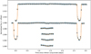 |
Fig. 1 Raw light curves of the four eclipses and the two phase curves measured by CHEOPS. The represented data were extracted byaperture photometry by the mission data reduction pipeline for a circular aperture radius of 25 pixels. Each data set is shifted upward with respect to the one observed before for visualisation purposes. The raw data points are shown in blue and binned once per CHEOPS orbit (black). The orange solid line is the best-fit model obtained with the modelling described in Sect. 4. The six observations are represented as a function of time since inferior conjunction according to the best-fit parameter values. |
3.2 Data reduction
3.2.1 Aperture photometry
All CHEOPS observations were processed with the latest version of the Data Reduction Pipeline (DRP), tagged version 13.1.0. We based the analysis presented in this work on these output photometric light curves that were produced following a procedure described in detail by Hoyer et al. (2020) and summarised below.
The first step of the data processing is referred to as calibration and aims to correct the images for the effects related to the detector and the optics. It consists of subtracting the bias offset of the CCD, converting the digital counts back to electrons (gain), correcting for the non-linear response of the read-out electronics, subtracting the contribution of the dark current, and, finally, correcting for the photo-response non-uniformity (flat field). The reference files on which the calibration correction is based have been produced during the on-ground calibration campaign performed on the CHEOPS payload before launch (Chazelas et al. 2019; Deline et al. 2020).
The second step is called the correction step and removes the spurious effects such as hits on the detector by high-energy particles (cosmic rays), background level caused by stray light, and smearing trails of bright close-by stars induced by the CCD read-out.
The CHEOPS DRP applies an aperture photometry method on the corrected images that consists of determining the location of the PSF centre (using an iterative centroiding technique) and counting the flux in electrons that falls within a given radius from this centre. The DRP provides photometric light curves for four different aperture radii: a default radius of 25 pixels, a small radius of 22.5 pixels, a large radius of 30 pixels, and an optimal radius that depends on the target observed1. The optimal aperture is designed to maximise the signal-to-noise ratio of the photometry and to minimise the contamination from nearby field stars based on simulations generated by the DRP using the Gaia catalogue (Gaia Collaboration 2021b) and a CHEOPS PSF template.
The photometric contamination from nearby stars as estimated by the DRP in the simulations has two components: the direct contamination and the smearing trails. The direct contamination is caused by nearby stars with PSF falling entirely or partly inside the photometric aperture. The associated signal is a positive offset with usually small variations that are in phase with the rolling of CHEOPS around the line of sight. If the offset is significant, it must be accounted for as it dilutes the flux from the target and might lead to underestimate the transit depth for instance. The smearing trails are vertical features above and below the nearby star PSF on the CCD. As the field of view rotates, the nearby stars move on the CCD and the trails enter the aperture periodically, contaminating the photometry. In most cases, both contributions can be corrected as a function of the roll angle of the spacecraft (provided in the light curve products of the DRP). In the case of WASP-189 observations, the brightest nearby stars have magnitude differences larger than 7.8 in the Gaia G band. They are expected to induce a direct contamination in the aperture smaller than 0.076% with variations of the order of 0.001%, and a signal due to smearing trails not greater than 0.021%. We thus consider that the photometric dilution has a negligible effect on relative photometric features (e.g. transits or eclipses). The associated variations, however, are comparable to the estimated photometric precision of the data (signal-to-noise ratio of the order of unity) and are corrected in the analysis as a function of the roll angle of the spacecraft.
During the full reduction process, the DRP runs diagnosis to determine if the data are valid according to several criteria: the location of CHEOPS with respect to the SAA, the values of various thermal sensors, the angular separations between the line of sight and three bodies (the Earth, the Moon, and the Sun), and the number of cosmic ray hits on the detector. If one of these criteria is out of range, the image is flagged accordingly. The DRP team recommends discarding all flagged images from photometric analyses.
Figure 1 shows the raw light curves obtained for the default aperture (radius of 25 pixels). For each observation, we estimate the photometric precision by computing the median absolute deviation (MAD) of the flux jumps df = fi+1 − fi to be robust to outliers and to remove correlated signals (e.g. transit, eclipse, stellar activity). The root-mean-square (rms) noise level  of the observation is then derived with the following formula:
  , with erf−1 being the inverse error function. This technique allows us to find results consistent with the ones computed from best-fit residuals (see Sect. 5.4). We find that the photometric precision of all observations are very similar, with values at the raw cadence (33.6 s) for the four eclipses and the two phase curves of 81.3 ppm, 89.8 ppm, 90.5 ppm, 93.9 ppm, 92.6 ppm, and 93.3 ppm, respectively. When applying the same method to several 1-h-long windows, we find median noise levels per 1-h bins of 11.3 ppm, 11.5 ppm, 10.8 ppm, 11.2 ppm, 12.1 ppm, and 12.1 ppm, respectively.
3.2.2 PSF photometry
In addition to the aperture photometry provided by the CHEOPS DRP, we cross-checked our analysis and the results against another photometric extraction technique, PSF photometry. This method consists of fitting the images witha two-dimensional template PSF in order to determine the amplitude of the signal and derive the flux.
We used a software package called PIPE, developed specifically for CHEOPS. The code is available on GitHub2 and will also be extensively described in Brandeker et al. (in prep.).
PIPE first derives a PSF template library from the observed sub-arrays and imagettes, using a principal component analysis (PCA). The first five principal components (PCs) together with a constant background are then used to best fit the PSF of each image using a least-squares minimisation. The number of PCs to use is a trade-off between following systematic PSF changes and overfitting the noise, but the derived photometry changes only marginally. The principal advantage is instead that the PC coefficients can be used to track PSF changes and correct for the so-called ramp effect (Sect. 4.3).
Apart from serving as an independent extraction method, PIPE has the advantage of being more robust against cosmic ray hits and telegraphic pixels, since these can be identified and flagged as statistically inconsistent with the PSF and thereby masked. Another advantage with PSF fitting is that accurate photometry can be extracted at faster cadence from the smaller imagettes. Since a large annulus around the target to measure the background is not required, it is simultaneously fitted with the PSF.
PIPE provides the photometric light curves together with the computed PSF coordinates, the background level and the relative weights UX of the first five principal components of the PSF PCA. Similarly to the DRP, images can be flagged for several reasons, such as a centroid far away from the median centroid, high level of bad pixels, or poor PSF fit.
Following the method described in the previous section, we obtain an estimate of the photometric precision that is very similar to the aperture photometry, albeit slightly better. At the raw cadence (33.6 s), one obtains 76.9 ppm, 84.4 ppm, 86.8 ppm, 88.6 ppm, 86.6 ppm, and 86.6 ppm for the four eclipses and the two phase curves, respectively. When considering 1-h-long windows, one reaches 10.8 ppm, 11.0 ppm, 11.1 ppm, 10.6 ppm, 11.5 ppm, and 11.2 ppm, respectively.
4 Light-curve analysis
4.1 Outlier removal
Prior to the analysis of the light curves, we perform a filtering of the data by first discarding all points flagged during the photometric extraction process, either aperture photometry from the DRP or PSF photometry from PIPE. The flagged data points represent 458/12 770 images (3.59%) for the aperture photometry and 493/12 770 (3.86%) and 2351/89 390 (2.63%) for PSF photometry on the sub-arrays and imagettes, respectively.
In addition, we apply two other criteria to identify data points as outliers and discard them. The first criterion is related to the level of background in the images. The change of background level is mostly due to variations in the amount of stray light entering the telescope along the orbit of CHEOPS, with the main sources of stray light being the Earth and the Moon. All observations are affected by a periodic increase of background level before and after Earth occultations. As mentioned in Sect. 3.1, the second and third eclipse observations of WASP-189 show much higher background levels (up to 10 times the nominal values) when compared to the other eclipse and phase-curve time series. While inspecting the housekeeping parameters for possible correlations, we noticed that these extreme background values resulted in an unexpected effect on photometry. As shown in Fig. 2, the measured flux becomes suddenly strongly anti-correlated with the background level above a given background value. This effect is present for all photometric apertures (DRP) as well as in the PSF photometry of sub-arrays (PIPE). However, it is not visible in the PSF photometry of imagettes, possibly due to the higher photometric noise of the data linked to the shorter cadence. We checked the moon separation for these observations and it appeared to be greater than 140deg, and similar to the one of the first phase curve. The fourth eclipse had the smallest moon separation of the whole data set (~ 35deg) but shows no extreme background levels. As this correlation is not yet understood and being investigated, we decided not to correct for it, but to clip out data points with background levels above a threshold that varies with the extraction technique (see Table A.1). This step results in discarding 45/3321 points (1.36%) for the two smallest apertures (22.5 and the default 25 pixels), 65/3321 points (1.96%) for the two largest apertures (30 and the optimal 40 pixels), and 52/3310 points (1.57%) for the PSF photometry on sub-arrays.
The second criterion is a sigma-clipping approach that differs slightly between eclipses and phase curves. Both methods rely on an estimate  of the noise level using a method robust against outliers that fits a Gaussian distribution to the histogram of the data and computes
  from the Gaussian width. For the eclipses, we normalise each individual observation by its median. We then perform a least-squares fit of the data with a linear trend for each observation and a common eclipse model from batman (Kreidberg 2015). Points beyond
  from the median value of the residuals are flagged as outliers. For the phase curves, both time series are normalised by their global median value. The model used to de-trend the data is a combination of a symmetric transit model (no GD) from batman and a single slope. For the DRP and PIPE sub-array photometry, data points are discarded when off by more than
  from the residual median. The sigma-clipping limit is reduced to
  for the PIPE light curves obtained from imagettes. The number of outliers flagged in the aperture photometry is 33/12 267 points (0.27%), 39/12 267 points (0.32%), 43/12 247 points (0.35%), and 55/12 247 points (0.45%) for the 22.5-, 25- (default), 30-, and 40-pixel (optimal) aperture radii, respectively. For the PSF photometry, we identify 10/12 225 points (0.08%) as outliers for sub-arrays and 15/87 039 points (0.02%) for the imagettes.
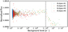 |
Fig. 2 Flux extracted with aperture photometry (DRP, aperture of 25 pixels) as a function of the image background levels for the four eclipse observations of WASP-189 b. This figure highlights the unexpected anti-correlation occurring above a given background value. The vertical dotted black line shows the threshold used to discard data points. |
4.2 Flux normalisation
The analysis of the photometric time series starts with the normalisation of the measured flux before modelling the systematics and astrophysical signals. As expected, the changes of observation conditions that occurred in-between eclipse observations (see Sect. 3.1) modified the absolute stellar flux measured with CHEOPS. The location of the PSF and the temperatureof the detector affect the flux repartition on the CCD (PSF shape) and the conversion factor from photo-electrons to digital units(gain of the read-out electronics), which in turn have an impact on the measured photometry. In order to account for this effect, we decided to include in our model an individual normalisation factor for each of the six eclipse and phase-curve observations that is applied before any of the data analysis steps described hereafter.
4.3 Systematic noise
The first systematic noise to be mentioned is specific to CHEOPS and is related to the rotation of the spacecraft around the Earth. In order to guarantee the thermal stability of the detector, the passively cooling radiator of the instrument must never face the Sun nor the Earth, which implies a continuous rolling of the spacecraft around its pointing direction with one full rotation per orbit. This nadir-locked orientation implies a rotation of the field of view around the target PSF, at a rate not necessarily constant, which causes nearby stars and stray light sources to move around and induce a periodic photometric noise. We implement a modelling of this systematic effect using the first terms of the following Fourier series:
 (1)
(1)
where θroll is the roll angle of CHEOPS provided in the data, and ai and bi are free parameters. We chose to limit the model to the first five terms of the series (N = 5 in Eq. (1)) as a trade-off between the quality of the fit, the number of parameters and to avoid overfitting the data. In addition, we implemented one model for the four eclipse observations and another for the phase-curve observations, or in other words, one set of coefficients  for the eclipses and one set
  for the phase curves. This decision is motivated by the fact that there is a gap of nearly 70 days between the eclipse observationsand the phase-curve observations. Over this two-month time span, the Earth moves significantly around the Sun, modifying its position with respect to WASP-189 in the field of view of CHEOPS. As a consequence, the photometricsystematics associated with the roll angle are different and could not be modelled by the same set of coefficients.
Another well-known systematic effect in the CHEOPS data sets is the so-called ramp effect. The source of this ramp is a thermo-mechanical distortion of the telescope tube that induces variations in distance and orientation of various optical components, including in particular the secondary mirror. This distortion is hard to predict as it depends on the orientation of the spacecraft with respect to the Sun during the observation preceding the one being analysed. The ramp has been extensively studied, andit has been found that (a) its duration can last up to more than 10 h with a behaviour similar to that of a thermal relaxation (exponential decay), (b) its photometric effect is correlated with the shape of the PSF, and (c) its photometric effect is correlated to the outputs from several thermal sensors, and in particular one referred to as thermFront_2. The study also concluded on a possible modelling of the effect as a linear relationship between theflux and the thermFront_2 temperature (Maxted et al. 2021). Based on this conclusion, we included a modelling of the ramp effect as a linear relationship between the flux and the telescope temperature as follows:
 (2)
(2)
where TthermFront_2 and ΔTthermFront_2 are the thermFront_2 temperature and its deviation from its median value respectively, and ctherm is a free parameter defining the strength of the correlation.
To account for other long-term systematic effects, we included a trend model for each observation. This model includes a linear slope with time for each data set, plus an additional quadratic trend for each of the eclipse observations, as shown in the following equation:
 (3)
(3)
where t is the time, t0 is the mid-time of each observation, c2 and c1 are the quadratic and linear trend coefficients for each observation (c2 = 0 for the phase curves). The nature of the corrected trends is not clearly determined and could be due to imperfect instrumental long-term stability, stellar activity or both. However, in light of the modelling of stellar activity in the phase curves discussed in Sect. 4.5, we strongly suspect that most of the trends in the eclipse observations are of stellar origin, but this could not be assessed given the short duration of each observation.
Based on the available housekeeping data, we performed an extensive study on possible correlations between the photometry and all the other parameters. We found no correlation other than the ones mentioned before that required modelling and correction.
4.4 Planetary model
The modelling of the photometric signal from WASP-189 b along its orbit is decomposed in three contributions that are described below. The first and second contributions are the transit model, for when the planet passes in front of the gravity-darkened star, and the eclipse model, for when the planet is hidden by the star. The third contribution is the phase-curve model that describes the flux received by the observer from the planetary surface as a function of its position around the star.
4.4.1 Transit model with stellar gravity darkening
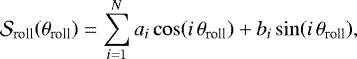
The fast-rotating nature of WASP-189 causes the centrifugal force to have a non-negligible effect with respect to the surface gravity. As a consequence, the effective surface gravity at the stellar equator is smaller than the one at the poles and the star becomes oblate. Based on the von Zeipel theorem (von Zeipel 1924), one can show that the radiative flux at a given latitude on the rotating star is proportional to the local effective surface gravity (e.g. Maeder 2009), and this implies the following relation:
 (4)
(4)
where  and Tpole are, respectively, the temperatures at a given colatitude ϑ and at the poles (ϑ = 0),
  and geff,pole are, respectively, the effective surface gravities at the colatitude ϑ and at the poles, and β is the GD exponent. The value of β is 0.25 for a purely radiative envelope but can deviate from the theory as measured for the star Altair (β = 0.190 ± 0.012, Monnier et al. 2007). The previous equation shows that, as the stellar rotation reduces the local effective gravity, the equator gets cooler and thus appears darker than the poles. The GD leaves a peculiar photometric signature when a planet transits in front of its star and hides regions with varying brightness, leading to asymmetric transit light curves when the orbit is misaligned.
As shown by Lendl et al. (2020), the transit light curve of WASP-189 b shows such GD features and one must account for this effect in the modelling of the data. In our analysis, we make use of pytransit3 (Parviainen 2015), version 2.5.13, which provides gravity-darkened transit models implemented based on Barnes (2009)4. The base assumption of various equations of the code is that the gravitational potential follows a Roche model, which is equivalent to assuming that only the outer layers of the star are distorted by rotation, meaning that the inner layers are spherical, hence producing the same gravitational potential as if the whole mass were concentrated at the centre of the star. pytransit represents the star as a discretised oblate sphere and computes the transit luminosity dip with a discretised planetary disc crossing and partially hiding the stellar object projected onto the plane of the sky. The effective surface gravity geff at each point on the stellar surface is evaluated from the Newtonian gravity force and the centrifugal force:
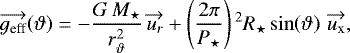 (5)
(5)
where G is the universal gravitational constant, M⋆ is the stellar mass, rϑ is the distance from the stellar centre of thepoint considered, P⋆ is the rotation period of the star, R⋆ is the stellar radius, and ϑ is the colatitude of the point. The unit vectors  and
and  point outwards, inthe opposite direction to the stellar centre and perpendicularly to the spin axis of the star, respectively. The local stellar radius rϑ equals R⋆ at the equator and decreases down to
 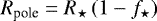 at the poles (ϑ = 0), where f⋆ is the stellar oblateness that can be expressed as a function of the stellar parameters:
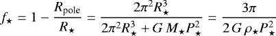 (6)
(6)
The temperature map of the star is computed from Eqs. (4) and (5) for every discretised surface point. The conversion from temperature to measured flux requires two additional elements, which are the flux emission spectrum  for a given temperature T and the instrument sensitivity or passband
  . pytransit provides the option to use synthetic spectra from the PHOENIX library (Husser et al. 2013), which are more suited than black-body laws to approximate the emission spectra of hot stars such as WASP-189. We compute the CHEOPS passband by combining the optical throughput of the telescope and the quantum efficiency of the detector that are both available as reference files in the CHEOPS mission archive5. The measured flux from a given point can then be computed after including the limb-darkening effect at the considered location:
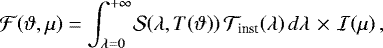 (7)
(7)
where  is the local flux, λ is the wavelength, ϑ is the colatitude of the point, and
  with x the normalised radial coordinate of the point. The term
  represents the local attenuation due to the limb darkening and is implemented in pytransit with the quadratic law
  , where u1 and u2 are the two limb-darkening parameters.
The implementation of pytransit limits the wavelength range of the PHOENIX spectra  from 300 to 1000 nm, while the CHEOPS passband
  covers the wavelength range from 330 to 1100 nm. As shown in Fig. 3, the combination of low stellar flux emission and poor CHEOPS sensitivity in the 1000–1100 nm range makes the contribution of this part of the spectrum in the integrated stellar flux small (<0.2%). Using pytransit and a black-body approximation for WASP-189, we estimated the effect of not accounting for wavelengths longer than 1000 nm to have an impact on the transit depth smaller than 0.2 ppm, which we considered to be negligible.
The pytransit model we implemented has the following parametrisation: the time of inferior conjunction T0; the period of the planetary orbit P; the planet-to-star radii ratio k = Rp∕R⋆; the normalised semi-major axis of the planetary orbit a∕R⋆; the inclination of the planetary orbit ip; the eccentricity e and the argument of periastron ω combined into two parameters  and
and  ; the two coefficients u1 and u2 of the quadratic limb-darkening law
  ; the projected stellar rotation speed
  ; the temperature of the stellarpoles Tpole; the stellar inclination i⋆; the projected orbital obliquity λp; the GD exponent β; the stellar equatorial radius R⋆; and the stellar mass M⋆. One must note that the time of inferior conjunction T0 might differ from the mid-transit time (mid-time between first and fourth contacts) in the case of oblate stars. For configurations where the orbit is misaligned but not perpendicular to the stellar equatorial plane (λp ≠90deg) and the impact parameter isnot zero (ip≠90deg), the oblateness of the star will cause a shift in mid-transit time with respect to T0 due to a late ingress or an early egress depending on the system orientation. The parameter R⋆ is the stellar radius at the equator and is the one used to normalise the planet radius Rp and the semi-major axis a and to compute two key parameters of the GD effect: the rotation period and the density of the star. The orientation of the planetary system is fully described by the three angles ip, i⋆, and λp, which need to be unambiguously defined in the case of GD. The convention on angular geometry used in this work is detailed in Fig. B.1. The stellar inclination is allowed to vary from 0deg (north pole on) to 180deg (south pole on). The orbital inclination ip is also defined on the interval
 ![Mathematical equation: $\left[0, 180\right]{\deg}$](/articles/aa/full_html/2022/03/aa42400-21/aa42400-21-eq42.png) with ip = 90deg corresponding to a transit through the center of the stellar oblate disc. The projected orbital obliquity λp varies in the
with ip = 90deg corresponding to a transit through the center of the stellar oblate disc. The projected orbital obliquity λp varies in the ![Mathematical equation: $\left[-180, 180\right]{\deg}$](/articles/aa/full_html/2022/03/aa42400-21/aa42400-21-eq43.png) range and affects the orientation of the planet transit path around the centre of the stellar oblate disc.
range and affects the orientation of the planet transit path around the centre of the stellar oblate disc.
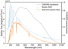 |
Fig. 3 Synthetic SED from the PHOENIX library (Husser et al. 2013) of a star similar to WASP-189. The stellar properties are an effective temperature Teff = 8000 K, a surface gravity logg = 4.0, and a solar metallicity. The stellar SED in blue is represented over the CHEOPS passband (330–1100 nm) shown as a black dotted line. The effective SED as seen by the CHEOPS instrument is the solid orange line, for which one can see that most of the energy lies within the 400–800 nm range and the contribution beyond 1000 nm is marginal. |
4.4.2 Eclipse model with an oblate star
Similarly to transits (see Sect. 4.4.1), the shape of the light curve during the occultation of the planet by its host will be affected by the oblateness of the star, causing a shift of the mid-eclipse time with respect to the time of superior conjunction and a change of shape of the ingress and egress. We note that this effect will be even more pronounced for grazing eclipses (and transits), but this does not concern the case of WASP-189 b.
For our analysis, we implemented an eclipse model based on the gravity-darkened transit model from pytransit to be consistent with the oblateness inferred by a given set of parameters. The model is the same as the transit model described in the previous section, with a few changes in the parameter values, as detailed below. The value of the time of inferior conjunction T0 is replaced by the time of superior conjunction, which is half an orbital period after T0 for circular orbits and can be computed from Kepler’s equation, relating the mean and eccentric anomalies, for eccentric orbits. The values of the limb-darkening coefficients u1 and u2 and the GD exponent β are set to zero to generate a uniform oblate stellar disc. The value of the argument of periastron ω, the inclination of the planetary orbit i and the projected orbital obliquity λp are modifiedas if the system were being observed from the other side. This transformation leads to the following sets of parameters: ωecl = ω + π, ip,ecl = π − ip, and λp,ecl = −λp.
The generated light curve corresponds to a transit in front of a uniform oblate stellar disc and has to be normalised to obtain the eclipse model for a fast-rotating star. The normalisation is performed so that the flux when the planet is fully occulted is 0, and the out-of-eclipse flux is equal to 1 (see Fig. 4). The normalised eclipse light curve is then multiplied by the phase-curve signal computed in the next section, which defines the eclipse depth.
4.4.3 Phase-curve signal
The phase-curve model used in this work is analytical and assumes the planet is a perfect Lambertian reflector (isotropic scattering) with a given geometric albedo Ag, and the thermal emission is approximated by a sinusoidal function of the planetary phase. To describe the orbital phase of the planet, we defined the phase angle of the planet ![Mathematical equation: $\alpha={\arccos}\!\left[-\sin\!\left(\omega+\nu\right)\sin\!\left(i_{\textrm{p}}\right)\right]$](/articles/aa/full_html/2022/03/aa42400-21/aa42400-21-eq44.png) , where ω is the argument of periastron, ν is the true anomaly, and ip is the orbital inclination. The values of the phase angle range between 0 at superior conjunction and π at inferior conjunction. The reflected flux component due to the isotropic reflection of the stellar light off the planetary atmosphere can be written analytically (Sobolev 1975; Charbonneau et al. 1999):
, where ω is the argument of periastron, ν is the true anomaly, and ip is the orbital inclination. The values of the phase angle range between 0 at superior conjunction and π at inferior conjunction. The reflected flux component due to the isotropic reflection of the stellar light off the planetary atmosphere can be written analytically (Sobolev 1975; Charbonneau et al. 1999):
 (8)
(8)
where F⋆ is the stellar flux, Ag is the geometric albedo, Rp is the planetary radius, a is the semi-major axis, e is the eccentricity, ν is the true anomaly, and α is the phase angle. The thermal emission flux is approximated by the following function of the phase angle:
 (9)
(9)
where Fday and Fnight are the planetary fluxes of the dayside and the nightside, respectively, and
![Mathematical equation: \begin{equation*}\alpha_{\textrm{therm}}={\arccos}\!\left[-\sin\!\left(\omega+\nu-\phi_{\textrm{therm}}\right)\sin\!\left(i_{\textrm{p}}\right)\right],\end{equation*}](/articles/aa/full_html/2022/03/aa42400-21/aa42400-21-eq47.png) (10)
(10)
with ϕtherm being the phase shift of the thermal emission accounting for hotspot offset. In total, our phase-curve model makes use of four parameters in addition to the ones already provided to the transit model described in Sect. 4.4.1: the geometric albedo Ag, the planet dayside and nightside fluxes, and the hotspot offset ϕtherm.
In the framework of this analysis, we also used another phase-curve model with a more complex implementation. The reflective component was more generic and allowed a divergence from a Lambertian profile as described in Heng et al. (2021). The thermal emission of the planet was computed from 2D temperature maps and integrated in the CHEOPS passband as detailed in Morris et al. (2022). This approach involved more free parameters and provided inconclusive results: the reflective component was consistent with a Lambertian profile and the thermal map was not constrained mostly due to the strong degeneracy between reflected light and thermal flux. We thus opted for the model with a Lambertian reflector and a sinusoidal thermal phase curve.
In addition to the reflective and thermal flux of the phase-curve model, we implemented the possibility to fit for the ellipsoidal variations (Mazeh 2008) and the Doppler beaming (Maxted et al. 2000), both approximated by sinusoidal functions:
 (11)
(11)
 (12)
(12)
where ν is the true anomaly, ω is the argument of periastron, ip is the orbital inclination, and Aell and Abeam are the semi-amplitudes of the ellipsoidal variations and the Doppler beaming, respectively.
The combined model of the light curve including the transit and eclipse models can be expressed as follows:
 (13)
(13)
where Ftra is the gravity-darkened transit light curve, Frefl and Ftherm are the reflected light and thermal emission from the planet, Fecl is the normalised eclipse model, and Fell and Fbeam represent the contributions from ellipsoidal variations and Doppler beaming.
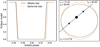 |
Fig. 4 Eclipse models with and without accounting for the oblateness of the host star. The parameters used in this example are the ones reported in Lendl et al. (2020) except for the stellar rotation speed (increased by a factor of 2 to enhance the effect of rotation), the projected orbital obliquity (set to 40deg), and the orbital inclination (set to 93deg). The left panel shows the light curves normalised by the out-of-eclipse flux for the same system orientation with an oblate stellar disc (solid black line) and a spherical star (orange dashed line). On the right we show a projected view of the system during the eclipse event. The black ellipse and the orange dashed circle show the limb of the star in both cases with the same colour code. The path of the planet is represented by the straight black line and arrows, with the planet being to scale (small black disc). |
4.4.4 Light-travel time
The light-travel time (LTT) across the planetary system is accounted for in the model used in this work. The observation times are converted into reference times by correcting for the light-travel time along the projected distance between the current planet position andits position at inferior conjunction. This choice of reference frame allows us to synchronise the time of inferior conjunction T0 in both time frames. For eccentric orbits, such a correction is slow as it has to be solved numerically, but fortunately it simplifies into an analytical formula for circular orbits:
![Mathematical equation: \begin{equation*}t_{\textrm{ref}} = t_{\textrm{obs}} - \frac{a}{c}\,\left[1-\cos\!\left(2\pi\frac{t_{\textrm{obs}}-T_0}{P}\right)\right]\,\sin\!\left(i_{\textrm{p}}\right),\end{equation*}](/articles/aa/full_html/2022/03/aa42400-21/aa42400-21-eq51.png) (14)
(14)
where tref is the time corrected for LTT, tobs is the observation time, a is the semi-major axis, c is the speed of light, T0 is the time of inferior conjunction, and P and ip are the orbital period and inclination. In this work, we always use Eq. (14) for LTT correction, even in the cases of non-zero eccentricity, as the orbit of WASP-189 b is expected to be close to circular (e ~ 0). This approximation avoids the use of slow numerical implementation. The expected amplitude of the correction is of the order of 50 s, which is the LTT between superior and inferior conjunctions. In practice, the transit, eclipse, and phase-curve models (Sects. 4.4.1–4.4.3) of data points observed at times tobs are computed using the corresponding LTT-corrected times tref.
4.5 Stellar variability
In addition to the instrumental systematics and the planet-related signal, the photometric time series feature another flux variability that we studied carefully before including a model for it. Figure 5 shows the raw flux variations after the removal of outliers (see Sect. 4.1) and the de-trending of a linear slope, where the variability is visible on top of the phase-curve signal from the planet. The first striking aspect is the absence of variability in the second phase curve while its detection is unambiguous in the first one, as revealed by the Lomb–Scargle periodograms (Lomb 1976; Scargle 1982) visible in the same figure. In addition, the maximum of the peak is located at a period of 1.19 days with a full width at half maximum of 0.43 days, which is consistent with the stellar rotation period of 1.24 days computed based on Lendl et al. (2020). We computed the spectral window of the observations to see how the sampling and gaps in the data impact the periodogram. The spectral window shows peaks corresponding to the orbital period of CHEOPS and its harmonics. This means these peaks are induced jointly by the photometric modulation with the roll angle of the spacecraft and the observation gaps due to Earth occultation and SAA crossings. Other peaks at longer periods are visible in the spectral window of the observations but none matches the signal at 1.19 days (see Fig. 5).
The spectral type and temperature of WASP-189 places it at the limit between stars with and without chromospheres and coronae (Fossati et al. 2018). Therefore, the nature of the stellar outer envelope is not well defined and might be either convective or radiative, which in turn implies the presence or absence of stellar spots, respectively. In the former case and the presence of spots, the stellar rotation is expected to create a photometric signature that could resemble the one observed in this time series. On the other hand, if the outer envelope is radiative, the lack of strong superficial magnetic activity leads to an absence of stellar spots and another mechanism is necessary toexplain photometric variability in phase with the stellar rotation. Recent asteroseismologic studies (Balona 2019; Trust et al. 2020) based on long-term observations with the Kepler space telescope (Koch et al. 1998; Borucki et al. 2010)and the Transiting Exoplanet Survey Satellite (TESS – Ricker et al. 2015) argue in favour of the presence of inhomogeneities of unknown origin at the surface of hot stars that could explain photometric variability matching the stellar rotation. As shown in the bottom panel of Fig. 2 of Trust et al. (2020), the photometric variability of the A-type star KIC 6192566 measured by Kepler is remarkably similar to the one observed for WASP-189, with a strong modulation matching the stellar rotation period that nearly disappears on a timescale of a few days, before reappearing. Lee & Saio (2020) recently provided another possible explanation for such a photometricvariability. They show that, when the convective core of an early-type star rotates slightly faster than its radiative envelope, it can excite non-radial pulsations (gravity modes) through resonance couplings. The frequency of the oscillation would then be at the rotating speed of the core, which is almost identical to the one of the outer layers.
The properties of WASP-189, namely its surface gravity log g and its effective temperatureTeff, places it in the instability strip where about 50% of the stars are expected to be hybrid δ Scuti - γ Doradus pulsators (Uytterhoeven et al. 2011). δ Scuti stars exhibit pulsations with periods typically ranging from dozens of minutes to several hours, while the γ Doradus variability is on longer timescales ranging from half a day to a few days. Therefore, γ Doradus pulsation modes could also explain the photometric variability seen in the CHEOPS phase curves. However, the surface gravity and effective temperature of the star are compatible with those of hybrid pulsators presenting both types of pulsations, albeit more in favour of δ Scuti modes in this case. Based on the Lomb-Scargle periodograms shown in Fig. 5, peaks with periods shorter than 6 h are exact harmonics of the CHEOPS orbital period and cannot be attributed to δ Scuti pulsations. This leaves only the mode at 1.19 days to be compatible with γ Doradus pulsations, but it seems unlikely that only a single frequency would be visible. For completeness, we ran a non-adiabatic oscillation computation of a stellar model of WASP-189 to determine which types of modes are expected to be excited, as well as their oscillation frequencies. We used the non-adiabatic code MAD (Dupret 2001; Dupret et al. 2005), with the inclusion of a time-dependent treatment for the interaction of convection with pulsation. The results show δ Scuti oscillation modes are unstable for this stellar model at frequencies between 225 and 500 μHz, or periods between 30 and 75 min, but none in the γ Doradus regime that could explain the peak observed in the data.
Based on this study on the possible origin of the photometric variability observed in the CHEOPS phase curves of WASP-189 b, we attributed the signal to the stellar rotation and decided to model it with a Gaussian process (GP) to account for its imperfect periodic nature. We implemented the GP model based on the code celerite (Foreman-Mackey et al. 2017) and, more specifically, using the kernel corresponding to a stochastically driven damped harmonic oscillator (SHO kernel). This kernel is efficient at modelling quasi-periodic oscillations and is defined by three hyper-parameters S0, Q and P0 that drive the amplitude, the damping and the period of the oscillations, respectively. Q is called the quality factor and has to be greater than 0.5 for oscillations to occur. In this case, the damped period of the oscillations is given by  , which can be used to estimate the period really fitted by the GP model.
The GP is fitted simultaneously with all other components of the model described previously. However, a Gaussian process is not a parametric function as its output also depends on the fitted data. Therefore, at each iteration the GP model is applied to the data after normalisation and subtraction of all parametric components of the model. The likelihood of the global model to represent the data is computed during this last step and involves the inversion of the covariance matrix generated from the kernel and the error bars of the data points. During the likelihood computation, an additional parameter σw acting as a jitter term is added quadratically to the residual error bars (diagonal of the covariance matrix) in order to account for possible underestimation of uncertainties in the data.
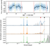 |
Fig. 5 Photometric variability observed in the two WASP-189 b phase-curve time series. Top: raw flux (blue points) variations in ppm around the median value after removing outliers, de-trending for linear slope and hiding in-transit (light red shaded area) and in-eclipse (light yellow shaded area) data. Black points are raw flux variations binned once per CHEOPS orbit (98.90 min). Bottom: Lomb–Scargle periodograms of the raw flux variations shown above. The top panel represents the power spectrum of the first phase curve observed for BJD < 2 459 020, while the mid panel corresponds to the second phase-curve observation (BJD > 2 459 021). The bottom panel is the periodogram of the combined phase-curve time series. The period range covered by each periodogram goes from the Nyquist period (twice the sampling time) to the durationof the time series, and thus encompasses all detectable periodicities. The coloured triangles in the top panel mark the periods of interest. The four leftmost ones (yellow) represent the fundamental (filled triangle) and harmonic (empty triangles) frequencies of the CHEOPS orbital period. The rightmost triangle (black) and the associated vertical dashed line correspond to the orbital period of WASP-189 b. The red triangle and dashed line mark the stellar rotation period of 1.24 days computed from Lendl et al. (2020). The grey shaded area corresponds to the spectral window of the observation (spectral power induced by the sampling and the gaps of the data). |
4.6 Prior probabilities of the model parameters
To fit our model to the data, we compute the probability of the full model (normalisation factor, systematic noise, planet-related signal and stellar variability) considering the measured data set. The probability is computed by combining the likelihood of all points to be represented by the model for a given set of parameter values, and the prior probabilities placed on the model parameters. We sample the posterior probability using a MCMC algorithm based on the code emcee described in Foreman-Mackey et al. (2013).
We describe here the choice of prior probabilities made for the models described in Sects. 4.2–4.5. Most of the parameters have broad uniform priors around the expected values with the only aim of reducing the size of the explorable parameter space and facilitate convergence of the fit. Choices of parameter prior probabilities motivated by other factors are detailed below. All prior probabilities are listed in Table 3 alongside the best-fit parameter values.
4.6.1 Eccentricity and argument of periastron
In the final analyses presented in this work, the eccentricity e used for the computation of the planet-related model is fixed to zero. This is justified by the fact that the orbits of ultra-hot Jupiters are expected to reach long-term stability on circular configuration. To support this choice of setting the eccentricity to zero, we ran a fit with free eccentricity values. We obtained from the results an upper limit at 3σ (99.93% confidence) on the eccentricity of 0.027. The largest values of e were reached for specific orbital configurations with the line of apsides along the line of sight (ω = 90 ± 180deg). When discarding these cases, the upper limit at 3σ on the eccentricity dropped to 0.005.
4.6.2 Limb-darkening coefficients
The values of the limb-darkening coefficients u1 and u2 are constrained by boundaries ensuring physically meaningful values of the intensity on the stellar disc, which correspond to a positive intensity everywhere on the stellar disc and a monotonically decreasing intensity towards the stellar limb. These conditions translate into three inequalities in the case of the quadratic limb-darkening law as detailed in Kipping (2013): u1 + u2 ≤ 1, u1 ≥ 0 and u1 + 2u2 ≥ 0. In addition to these boundaries, we included a prior probability on the coefficients, which corresponds to the likelihood of the quadratic limb-darkening law  for a given pair
  to represent a theoretical stellar intensity profile. This intensity profile is generated using the code LDCU6, which computes limb-darkening profiles and coefficients from two libraries of synthetic stellar spectra, ATLAS (Kurucz 1979) and PHOENIX (Husser et al. 2013), following the method detailed by Espinoza & Jordán (2015). In order to account for uncertainties σi on the stellar parameters, several profiles are generated by drawing stellar parameter set from normal distributions
  . Each profile is interpolated with a cubic spline over 100 evenly-spaced μ points as done by Claret & Bloemen (2011) to uniformly spread the weighting of the profile across the stellar disc. The likelihood
  is computed as a function of the χ2, which is the sum of the quadratic distance of the theoretical profile points to the evaluated profile
  , and the minimum χ2 value corresponding to the best possible fit of the theoretical profiles:
  . This value is added to the global log-likelihood value and acts as a penalty for coefficients that would generate a limb-darkening profile completely different from the best-fit to the synthetic atmospheric models. The inclusion of the limb-darkening likelihood in the MCMC runs was tested and validated as it resulted in a faster convergence of the exploration and a negligible effect on the final parameter values.
4.6.3 Gravity-darkening parameters
Prior probabilities are set on the parameters used to constrain the GD effects in the transit and eclipse models. The projected stellar rotation speed  , the temperature of the stellar poles Tpole, the stellar equatorial radius R⋆, and the stellar mass M⋆ have normal priors corresponding to the values and uncertainties listed in Table 1, with the temperature of the poles equal to the effective temperature. We let the stellar inclination i⋆ vary uniformly in the range
 ![Mathematical equation: $\left[0{-}180\right]{\deg}$](/articles/aa/full_html/2022/03/aa42400-21/aa42400-21-eq60.png) . We place a normal prior on the projected orbital obliquity λp based on the value derived from Doppler tomography by Anderson et al. (2018) (λp = 89.3 ± 1.4deg). Finally, we fix the GD exponent β to the valueprovided in Table 2 of Claret (2016) based on the stellar effective temperature, which gives β =β1∕4 = 0.22.
. We place a normal prior on the projected orbital obliquity λp based on the value derived from Doppler tomography by Anderson et al. (2018) (λp = 89.3 ± 1.4deg). Finally, we fix the GD exponent β to the valueprovided in Table 2 of Claret (2016) based on the stellar effective temperature, which gives β =β1∕4 = 0.22.
We note that, when allowed to vary freely, the parameters β and λp converge to values that are unphysical and inconsistent with Doppler tomography, respectively. This degeneracy justifies the use of prior probabilities from Doppler tomography as detailed in Sect. 5 of Hooton et al. (2022).
4.6.4 Phase-curve parameters
In the phase-curve model, we let the geometric albedo Ag vary freely within the theoretical Lambertian range ![Mathematical equation: $\left[0, 2/3\right]$](/articles/aa/full_html/2022/03/aa42400-21/aa42400-21-eq61.png) and the hotspot offset ϕtherm within the range
and the hotspot offset ϕtherm within the range ![Mathematical equation: $\left[-60, 60\right]\,{\deg}$](/articles/aa/full_html/2022/03/aa42400-21/aa42400-21-eq62.png) . We constrain the dayside flux Fday to positive values. We first ran an analysis allowing non-zero nightside flux that yields
. We constrain the dayside flux Fday to positive values. We first ran an analysis allowing non-zero nightside flux that yields  . We therefore fixits value to zero.
4.6.5 Ellipsoidal variations and Doppler beaming
The amplitudes of the ellipsoidal variations and the Doppler beaming are both fixed to zero. When fitted for, the amplitude of the ellipsoidal variations are degenerate with the GP modelling the stellar variability, especially in the second phase curve where the variability is nearly absent, and we obtain  ppm. Following the formula from Esteves et al. (2013) and using values from Lendl et al. (2020), we can estimate the order of magnitude of the semi-amplitude of the ellipsoidal variations:
 (15)
(15)
where αell is a coefficient of the order of unity and Mp is the mass of WASP-189 b. The value we obtain by fitting CHEOPS data is much larger than this estimation, and it can be explained by the fact that large amplitudes Aell create a signal in the second phase curve that mimics the variability modelled by the GP in the first phase curve. The global model has a higher likelihood given the ability of the GP to correct for this induced signal, even though its amplitude is not realistic. We thus decide to fix Aell to zero to prevent this effect from biasing the results of the final analyses. The amplitude of the Doppler beaming is consistent with zero when left free, so we remove a degree of freedom by fixing it to zero as well. We validate this choice by computing the expected amplitude following Esteves et al. (2013): Abeam ≈ αbeam K∕c ≈ 1 ppm, where αbeam is of the order of unity, K is the radial-velocity semi-amplitude, and c is the speed of light.
In addition, we performed model comparison by including Ellipsoidal variations, Doppler beaming, or both phase-curve components. We compared the different best-fit models using the Bayesian information criterion (BIC) and the Akaike information criterion (AIC). The model that minimises both the BIC and AIC is the one without Ellipsoidal variations or Doppler beaming. We report here the BIC and AIC differences with the best model: ΔBIC = 20.5 and ΔAIC = 13.1 for Ellipsoidal variations only, ΔBIC = 9.4 and ΔAIC = 2.0 for Doppler beaming only, and ΔBIC = 18.0 and ΔAIC = 3.2 when including both. These numbers further validate the choice to discard the contribution of Ellipsoidal variations and Doppler beaming from our final model.
Planetary parameters obtained with the model assuming a Lambertian reflector and approximating the thermal emission as a sinusoidal function of the phase angle.
4.6.6 Gaussian process
The last set of prior probabilities are placed on the Gaussian process hyper-parameters. The amplitude and damping hyper-parameters S0 and Q are sampledlogarithmically and allowed to vary in an interval aimed uniquely to reduce the size of the parameter space and improve convergence speed of the MCMC run. The undamped period of the oscillations P0 is constrained by a normal prior determined from the oscillation peak identified in the Lomb-Scargle periodogram (see Fig. 5), which corresponds to a distribution of 1.2 ± 0.2 days.
5 Results and discussion
In this section, we present the results we obtained from the analyses of the data sets. We performed several fits on all available light curves obtained with either aperture or PSF photometry. This represented a total of six light curves, with four aperture sizes provided by the DRP and two PIPE time series extracted from sub-array images and at higher cadence from imagettes. The results obtained from all light curves lead to consistent values for every planetary parameter. The best precision was reached in the cases of aperture photometry with the so-called default aperture size (aperture radius of 25 pixels) and PSF photometry on the sub-array images. Unfortunately, the gain in cadence provided by the imagettes did not provide additional constraints on the parameter values due to a too significant loss of precision. Even though the outcomes of the default aperture photometry and PSF photometry on sub-arrays were extremely similar, we noticed a slight improvement with the latter with some of the system properties better constrained. Therefore, in this work we present the best outcome of our analysis obtained with the MCMC analysis of the light curves extracted with PIPE from the 200 × 200-pixel subarray images. The MCMC sampling of the posterior distribution was performed using 128 chains with burn-in phases longer than 20 000 steps to ensure convergence of the algorithm, and sampling phases of 16 384 steps.
5.1 Planetary parameters
The values of the main parameters of our best fit are listed in Table 3. They are related to the architecture of the planetary system, the stellar activity or the ramp effect. The other parameters used to normalise and de-trend the light curve against time and roll angle have their best-fit values listed in Table C.1.
The system orientation is illustrated in Fig. 6, where the star is represented at its most probable inclination, and several planetary orbits sampled from the posterior distribution are shown.
All the fitted planetary parameters are consistent with values obtained in Lendl et al. (2020). We note that the quantities normalised by the stellar radius (k and a∕R⋆) are different, however. This is actually due to the fact that the stellar radius used for normalisation in Lendl et al. (2020) is the polar radius, while it is the equatorial radius in our approach. Comparing absolute values of the planetary radius Rp and the semi-major axis a show consistencies within 0.1 σ.
We note that the time of inferior conjunction T0 and the orbital period P are fully consistent with the values reported in Anderson et al. (2018). We obtain an exquisite precision on both parameters with fewer than 2 s for the period and an optimum T0, opt at about 4 s.
From the fitted parameters, we derive a series of other useful parameter values, including the eclipse depth that is the amplitude of the phase curve (reflected and thermal) at superior conjunction (ω + ν = 270deg). It is important to mention that the amplitudes of the reflected and thermal parts of the phase curve are degenerate, especially where the hotspot offset is zero and the full amplitude is the sum of both contributions. This is the case for WASP-189 b, and the degeneracy is strong, with either a high geometric albedo Ag and a low dayside thermal flux Fday with unconstrained ϕtherm values, or a more constrained offset for low Ag (see Fig. D.1). In order to provide reliable uncertainties on ϕtherm, the value reported in Table 3 is computed for Ag < 0.05, corresponding to a fully thermal phase curve. We find no indication for a hotspot offset from the sub-stellar point with the phase curve peaking at occultation.
The true orbital obliquity Ψp describes the relative orientation of the planetary orbit with respect to the spin axis of the star, and we compute it with the following angular relationship (see Fig. B.1):
![Mathematical equation: \begin{equation*}\Psi_{\textrm{p}}={\arccos}\!\left[\cos\!\left(i_{\textrm{p}}\right)\cos\!\left(i_{\star}\right)+\cos\!\left(\lambda_{\textrm{p}}\right)\sin\!\left(i_{\textrm{p}}\right)\sin\!\left(i_{\star}\right)\right],\end{equation*}](/articles/aa/full_html/2022/03/aa42400-21/aa42400-21-eq66.png) (16)
(16)
where ip is the orbital inclination, i⋆ is the stellar inclination and λp is the projected orbital obliquity. From the values of our MCMC runs, we obtain Ψp = 89.6 ± 1.2deg, which is fully consistent with a polar orbit.
Despite the convergence of the fit towards a well-defined system orientation, there remains a degeneracy inherent to gravity-darkened transit photometry. The following four sets of angular parameters will produce the same photometric signal:

From the observer’s point of view, the difference between configurations 1 and 2 (and between 3 and 4) is that one is the symmetric of the other with respect to the ‘vertical’ plane containing the line of sight and the spin axis of the star. Similarly, configuration 1 (respectively 2) is symmetrical to 3 (respectively 4) with respect to the ‘horizontal’ plane containing the line of sight and perpendicular to the vertical plane mentioned previously. Spectroscopic observations such as Doppler tomography can rule out two out of four configurations by measuring if the transiting planet is above the blueshifted or the redshifted hemisphere of the rotating star. In the case of WASP-189 b, Anderson et al. (2018) show by Doppler tomography that the polar orbit only goes over the redshifted hemisphere, which leaves only two possible scenarios, which are represented in Fig. 6. The second scenario (right-most panel of Fig. 6), where i⋆ > 90deg and the south stellar pole is visible, cannot be ruled out based on the data available, and it gives the same true orbital obliquity.
We constrained the stellar oblateness f⋆ of WASP-189 and were able to determine that its polar radius is about 2.9% smaller than its equatorial radius due to its fast rotation. This corresponds to a temperature difference of about 200 K between the poles (8000 K by construction) and the equator (~7800 K).
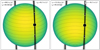 |
Fig. 6 Representation of the two possible orientations of the WASP-189 planetary system. The star is in its most probable state with the grey dashed curves marking constant stellar latitudes and with the north pole upward. In this representation, the stellar rotation causes the left and right hemispheres to appear blueshifted and redshifted, respectively. The stellar oblateness
|
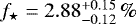
5.2 Phase-curve constraints on the planetary atmosphere
The light curve obtained after removing systematic noise and stellar activity assuming a Lambertian reflector and a sinusoidal thermal emission is shown in Fig. 7. The phase curve highlights the exquisite photometric precision of CHEOPS while the planetary eclipse and the asymmetric transit are visible. Figure 8 shows the corrected phase-folded data around the mid-transit time and clearly reveals the effect of GD on the transit shape. The uncertainty on transit and eclipse parameters is small compared to the uncertainty found on the phase-curve signal. This is due to the photometric variability attributed to the stellar activity that is not perfectly periodic and thus hard to disentangle unambiguously from the planetary signal.
As described in Sect. 5.1, we computed the hotspot offset ϕtherm reported in Table 3 for parameter sets probing a phase-curve model dominated by thermal emission (Ag< 0.05). We derived a hotspot offset consistent with zero (ϕtherm = −7 ± 17 deg). The precision on this parameter value is likely limited by the uncertainty on the phase curve induced by stellar activity.
As reported in Sect. 4.6, we fitted the data with the nightside flux as a free parameter and found a value consistent with zero. However, we also obtained a large upper uncertainty on Fnight with a 3 σ upper limit matching a uniform temperature distribution on the planet surface (Fnight ≈ Fday), which means a heat redistribution efficiency of ε = Fnight∕Fday ≈ 1. This results from the use of Gaussian processes to model the stellar activity: its flexibility was necessary to properly correct the associated signal, but with the downside of adding considerable degeneracies in the shape of the phase-curve model. Using the nightside flux we obtain when this parameter is free, we can nevertheless compute the heat redistribution efficiency in the CHEOPS passband  . Assuming a fully thermal phase curve (Ag → 0), we derive a smaller limit of
  (see Fig. 9). Both values are less than 1.5 σ away from 0 and have a 3 σ upper limit consistent with 1.
Due to the degeneracy between reflective and thermal components, we could not determine the contribution of each part in the absence of a significant hotspot offset. Therefore, we followed an approach assuming two extreme cases for the phase-curve amplitude.
We first considered the case where the amplitude of the eclipse is only due to reflected light without any thermal contribution from the planet. The conversion of the eclipse depth δecl into reflected light is done with Eq. (8) for a circular orbit (e = 0) and at superior conjunction (α = 0). It provides a maximum geometric albedo Ag,max = 0.42 ± 0.02, from which we compute a 3 σ upper limit (99.93% confidence) and determine that the geometric albedo of WASP-189 b is Ag < 0.48. This value is not inconsistent with other measured geometric albedos of ultra-hot Jupiters, even though these objects usually feature darkatmospheres with low reflectivity (Wong et al. 2021).
We then explored how the thermal emission contributes to the flux as seen through the CHEOPS passband. The power irradiating the planet is given by the following expression:
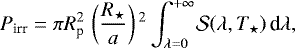 (17)
(17)
where Rp is the planet radius, R⋆ is the stellar radius, a is the semi-major axis, and  is the flux emission spectrum of the star as a function of its temperature T⋆ and the wavelength λ. We can compute the power absorbed by the planetary atmosphere
  , with AB being the Bond albedo. The power radiated away by the planet must equal the one absorbed if it is to be at equilibrium. Assuming the planet is a black-body radiator, we can derive a relationship between the average effective temperature of the planet
  and the irradiating power Pirr and obtain the following:
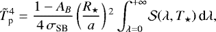 (18)
(18)
where AB is the Bond albedo and σSB is the Stefan-Boltzmann constant. The average effective temperature of the planet is given by 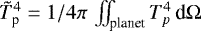 , where Tp is the local effective temperature in the planetatmosphere and dΩ describes a surface element of the atmosphere. Following the parametrisation of Cowan & Agol (2011), we define the dayside and nightside effective temperatures as functions of the heat redistribution efficiency ε and
  :
:
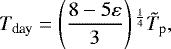 (19)
(19)
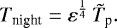 (20)
(20)
We computed the ranges of values of both temperatures when the Bond albedo and the heat redistribution efficiency are allowed to vary within ![Mathematical equation: $\left[0, 1\right]$](/articles/aa/full_html/2022/03/aa42400-21/aa42400-21-eq82.png) (see Fig. 10). We used the spectral energy distribution represented in Fig. 3 for the star and the median value reported in Table 3 for a∕R⋆. In the limit where no energy is absorbed by the planet (AB → 1), we retrieve a temperature of 0 K everywhere on the planet. When all the irradiating power is absorbed (AB = 0) and the heat redistribution is perfect (ε = 1), we obtain a uniform atmospheric temperature
(see Fig. 10). We used the spectral energy distribution represented in Fig. 3 for the star and the median value reported in Table 3 for a∕R⋆. In the limit where no energy is absorbed by the planet (AB → 1), we retrieve a temperature of 0 K everywhere on the planet. When all the irradiating power is absorbed (AB = 0) and the heat redistribution is perfect (ε = 1), we obtain a uniform atmospheric temperature  . The maximum dayside temperature is reached when AB = ε = 0, and one obtains Tday, max = 3355 ± 14 K for WASP-189 b.
From the dayside temperatures, we were able to calculate the corresponding eclipse depth in the CHEOPS passband with the following relationship:
 (21)
(21)
where Rp and R⋆ are the planetary and stellar radii, respectively,  and
and  are the fluxemission spectra of the planet and the star, respectively, and
  is the CHEOPS passband. Similarly to the computation of the effective temperatures, we used a black-body approximation for the planet, the spectral energy distribution of Fig. 3 for the star, and the median value of k = Rp∕R⋆ from Table 3. The values of Fday∕F⋆ are displayed in Fig. 11. We retrieve expected trends such as a low flux for high Bond albedo values and maximal dayside thermal flux when ε → 0.
It is noteworthy that the maximum dayside temperature Tday, max computed in the case of black-body emission only produces an eclipse depth of 68.5 ± 1.8 ppm in the CHEOPS passband, which is not enough to explain the measured  . The dayside temperature necessary to generate such a thermal flux is 3542 ± 14 K and corresponds to a negative Bond albedo (AB ≈−0.24 for ε = 0). From these values, it seems that a fully thermal emission with no reflected light cannot explain the eclipse depth measured with CHEOPS and this in turn implies a minimum geometric albedo Ag > 0.12 ± 0.02.
To further explore the limits on the dayside thermal flux, we computed a synthetic planetary emission spectrum using the radiative transfer code HELIOS (Malik et al. 2017, 2019). The model assumes a cloud-free atmosphere in chemical equilibrium with several sources of opacity as detailed in Lendl et al. (2020). The inputs used for the computation are a stellar emission spectrum from the PHOENIX library (Husser et al. 2013) as shown in Fig. 3 and the median values of the planetary parameters listed in Table 3. We also assumed that all the irradiating stellar power is absorbed by the planet (AB = 0) and that there is no heat redistribution (ε = 0). We obtain the SED represented in Fig. 12 with many emission lines in the blue end of the spectrum leading, in turn, to an increase of flux in the CHEOPS passband with respect to the black-body approximation.
We computed the dayside flux in the CHEOPS passband using the HELIOS emission spectrum for the planet in Eq. (21). The resulting eclipse depth is slightly larger than the black-body case with 77.0 ± 2.5 ppm. This value remains inconsistent with the measured eclipse depth by 3.5 σ and implies Ag > 0.08 ± 0.02.
In an attempt to maximise the modelled eclipse depth, we performed a final computation using the same HELIOS model for the planet but accounting for a cooler and oblate star. We used a stellar emission spectrum from the PHOENIX library (Husser et al. 2013)for a stellar temperature of 7800 K (minimum temperature reached at the equator) and reduced the size of the stellar disc by a factor 1 − f⋆ in Eq. (21) to account for its oblateness. These settings represent a lower limit of the received stellar flux (smaller cooler star) and maximise the detected eclipse depth up to 87.1 ± 3.1 ppm, which is marginally consistent (1.6 σ) with a fully thermal phase curve and no reflected light. However, this latest result corresponds to an extreme limit where AB = ε = 0 and the stellar flux is expected to be underestimated as we assumed a uniform photospheric temperature equal to the equatorial minimum. As a consequence, the numbers we obtain seem to point toward a non-zero geometric albedo, with a lower limit of Ag > 0.041 ± 0.026 in the most extreme case. These results are consistent with the temperatures reported by Lendl et al. (2020), where the dayside temperature computed with Ag = 0 exceeds the limit of stellar irradiating power.
In light of this study, it is difficult to explain the observed eclipse depth by pure thermal emission from the atmosphere of WASP-189 b. The conditions we considered to reach marginal consistency are extreme with the smallest and coolest possible star, and a full absorption of the stellar irradiation by the planet. Moreover, the heat redistribution inefficiency maximising the dayside temperature also implies a nightside temperature of nearly 0 K. Therefore, it seems very likely that the planetary signal is not purely thermal and that the atmosphere has a non-negligible reflective component in the CHEOPS passband. As we have shown in this study, deriving a precise lower limit on the geometric albedo strongly depends on the assumptions made on the star, the system architecture and the atmospheric properties of the planet. Nevertheless, it is noteworthy that the limit on the geometric albedo derived using the HELIOS emission spectrum is consistent with Ag ~ 0.1. Similar geometric albedos have been reported for comparable planets (Wong et al. 2021), even if the current atmospheric models struggle to explain the presence of reflective material at temperatures larger than 3000 K.
TESS (Ricker et al. 2015) will observe the WASP-189 system in April–May 2022 when covering sector 51. With its redder passband, TESS is more sensitive to planetary thermal flux than CHEOPS, and the planet-to-star flux ratio is expected to be even larger in the case of hot blue stars such as WASP-189. Thus, if the flux from WASP-189 b is mostly of thermal origin, the eclipse observed with TESS should be much deeper than the one reported in this work. Following the method described in this section, we computed the dayside thermal flux in the TESS passband as a function of AB and ε, similarly to Fig. 11. We estimate that TESS could measure an eclipse depth due to thermal emission up to 165 ± 4 ppm. Such a signal should be detectable with a precision of more than 3 σ when combining the eight-to-ten eclipses observed during the two TESS orbits (~ 27 days). An additional significant advantage is the long baseline of the observations, which will allow a more robust correction of the stellar variability. A precise determination of the eclipse depth in the TESS passband should provide an upper limit on the dayside temperaturecorresponding to a fully thermal phase-curve amplitude. If one assumes that both CHEOPS and TESS probe the same atmospheric layer, and hence the same temperature distribution, one could use this result to constrain the geometric albedo in the CHEOPS passband.
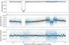 |
Fig. 7 Phase-folded phase curve of WASP-189 b after correction of instrumental systematics and stellar activity. This data set is obtained from a model assuming the planet is a Lambertian reflector and approximating the thermal emission with a sinusoid function. The data points de-trended from all systematics and stellar variability are shown in blue in the two upper panels. The mid-panel shows a zoomed-in view of the upper one to better visualise the phase-curve signal. The lower panel shows the residual after subtraction of the best-fit planet model. The black points represent the binned data with 100 bins per orbital period, which corresponds to a bin duration of about 40 min. The faded orange lines are 100 samples drawn from the posterior probability obtained from the MCMC run, and thus highlight the uncertainty we obtain on the best-fit model. |
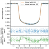 |
Fig. 8 Phase-folded transit light curve of WASP-189 b after correction of instrumental systematics and stellar activity. The top panel shows the normalised flux and two best-fit transit models with and without GD. The mid-panel (blue-point residuals) shows the best-fit residuals for the model accounting for GD. The bottom panel displays the residuals after removing a transit light curve without accounting for the gravity-darkened stellar photosphere. The black dashed line is the deviation of the model without GD from the model with GD. |
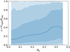 |
Fig. 9 Heat redistribution efficiency ε as a functionof the geometric albedo Ag. The median value of ε is represented by the blue curve and the shaded areas highlight the 1 σ, 2 σ, and 3 σ uncertainty range. The value of ε is computed as the nightside-to-dayside flux ratio measured by CHEOPS. Low values of Ag indicates low reflectivity and a phase-curve amplitude mostly due to thermal emission. The thermal contribution gets smaller for higher Ag where reflected light starts to be important. |
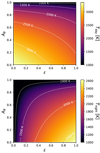 |
Fig. 10 Dayside (top) and nightside (bottom) effective temperatures of the atmosphere of WASP-189 b as a function of the Bond albedoAB and the heat redistribution efficiency ε. The lower limit of the colour scale is set to 1000 K for abetter visualisation. White dotted lines show isothermal profile across the (AB, ε) plane. The dayside and nightside temperatures are equal when ε = 1 and both go down to 0 K in the limit AB → 1. If the dayside temperature is 3000 K, then the Bond albedo values range from 0 to ~0.38, with corresponding values of the heat redistribution efficiency from ~0.59 to 0, respectively. In such a case, the maximum nightside temperature would be ~ 2250 K. |
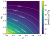 |
Fig. 11 Dayside thermal flux from WASP-189 b as a function of the Bond albedo AB and the heat redistribution efficiency ε. The flux Fday is normalised by the stellar flux F⋆. Both fluxes are computed as seen through CHEOPS passband. White dotted lines show constant flux ratios across the (AB, ε) plane. If the measured eclipse depth contains a thermal emission component with an amplitude 40 ppm, the Bond albedo may be as large as ~0.29 and as small as zero, and the corresponding heat redistribution efficiency would be zero and ~ 0.45, respectively. |
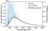 |
Fig. 12 Spectral energy distribution of the planet WASP-189 b. The high-resolution synthetic SED computed with HELIOS (Malik et al. 2017, 2019) is represented in light blue and assumes the irradiating power is fully absorbed and not redistributed (AB = ε = 0). The dark blue line is the HELIOS data averaged over bins of 5 nm. The black-body profile of the maximum dayside temperature Tday, max is shown inorange. We note that accounting for emission lines in the planetary spectrum leads to a different SED with respectto the black-body approximation, with more energy in the blue end. This affects the flux measured in the CHEOPS passband (black dotted line), with the dayside of WASP-189 b appearing slightly brighter. |
5.3 Stellar activity
We fitted the photometric variability observed in the phase curves with a Gaussian process and attributed to stellar rotation. The extracted variability, corrected from systematics and after subtraction of the planet model, is shown in Fig. 13, where several GP models drawn from the posterior distribution are shown. The signal is well fitted, especially in the first phase curve, and the flexibility of the Gaussian processes is used to adapt to the change of variability in the second part.
We combine the stellar inclination obtained from our analysis with the stellar radius and the projected rotation speed to compute the rotation period of WASP-189. The estimated period 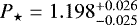 days matches the peak maximum measured from the Lomb-Scargle periodogram precisely (see Fig. 5) and supports the notion that stellar rotation is indeed the cause of the observed photometric variability.
The damped period of the GP is computed from the undamped period P0 and the quality factor Q and its value 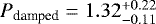 days is consistent at 1σ with the stellar rotation period. The large upper error bar seems to indicate that longer periods might be favoured, which can be caused by the absence of oscillations in the second phase curve.
Our results seem to indicate that the stellar rotation and the photometric variability fitted by the GP are related. If the stellar outerenvelope is convective, this likely indicates the presence of stellar spots on WASP-189. However, the nature of the outer envelope cannot be clearly assessed and could be radiative. In that case, the mechanism causing this phenomenon is not understood, either due to inhomogeneities on the stellar surface (Trust et al. 2020) or excited pulsation modes (Lee & Saio 2020), as discussed in Sect. 4.5.
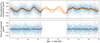 |
Fig. 13 Photometric variability attributed to stellar rotation as fitted by the Gaussian process. The upper panel shows in blue the time series corrected for instrumental systematics and the planet model, including transit, eclipse, and phase-curve signal. The residuals of the best-fit are represented in the lower panel (blue points). The data points binned once per CHEOPS orbit are shown in black. The faded orange lines are GP models sampled from the posterior distribution highlighting the uncertainty of the fit. The vertical dotted lines mark the time interval of the planetary transits (red) and eclipses (green). |
5.4 Photometric precision
The photometric performance of CHEOPS can be evaluated from the residual light curve after correcting for all systematic effects, the stellar activity and removing the planetary model (bottom panel of Fig. 7). The noise level in the residuals is evaluated over a given duration by computing the error on the mean of all data points in a time window of the considered duration. The window is moved across the whole time series to estimate the noise at different moments of the observation. The median of the noise levels computed for a given duration gives us a precise estimate of the photometric performances of CHEOPS. We compute the noise levels using five different methods, which will not be detailed here as it goes beyond the scope of this work; however, all give consistent results. Based on this approach, we evaluate the photometric precision of the CHEOPS observations of WASP-189 (A4-star of magnitude V = 6.6) to be 10 ppm over 1-h windows, and it goes down to 5 ppm over a 6-h window.
6 Conclusion
In this work, we perform the analysis of the CHEOPS observations of the WASP-189 system that cover four eclipse events and two full phase curves of the ultra-hot Jupiter. We fit the asymmetric transits with a model accounting for GD and oblateness of the fast rotating star. We measure a planetary radius of  , which consistent at 0.7 σ with the value 1.619 ± 0.021 RJ from Lendl et al. (2020), and constrain the stellar oblateness with a polar radius
  smaller than the equatorial radius. We also robustly determine the system orientation and find that WASP-189 b is on a polar orbit with a true orbital obliquity Ψp = 89.6 ± 1.2deg. The value is more precise and consistent at 0.9 σ with 85.4 ± 4.3deg found by Lendl et al. (2020). Combined with Doppler tomography, we narrow down the architecture of the system to two possible configurations where the planet transits in front of the receding hemisphere of the star: one with the north stellar pole visible, the other with the south pole visible.
We measure an eclipse depth of  and find no hints of strong atmospheric winds with a hotspot offset consistent with zero (− 7 ± 17 deg). Our value of the eclipse depth is consistent at 1.3 σ with the value 87.9 ± 4.3 ppm derived by Lendl et al. (2020). Our precision is similar despite two additional eclipses, and we attribute this to the presence of photometric variability. The stellar activity also prevents us from deriving precise constraints on the planet nightside flux or on the heat redistribution efficiency. We could not disentangle the contribution of reflected light and thermal emission to the phase curve amplitude, but we compute an upper limit on the geometric albedo in the CHEOPS passband (Ag < 0.48). Using synthetic emission spectra for both the star and the planet, we show that the brightness of WASP-189 b in the CHEOPS passband is only marginally explained by thermal emission alone and that it would require a Bond albedo of zero and an extremely inefficient energy redistribution. This conclusion is consistent with the work of Lendl et al. (2020), where the reported dayside temperature is 3435 ± 27 K and implies a negative Bond albedo (emitted planetary flux larger than stellar irradiating power).
From the transit fit, we infer the inclination of the host star and compute its rotation period ( ). This period matches the photometric variability detected in the data and attributed to stellar activity. As the properties of WASP-189 do not allow to assess the nature of the outer envelope, we propose several possible explanations. If the outer envelope is convective, then the presence of spots is the most probable cause for the photometric variability. In the case of radiative envelope in A-type stars, we mention two mechanisms that could explain the observations: inhomogeneities on the stellar surface or pulsation modes excited by resonance couplings between the convective core and the radiative envelope.
The CHEOPS time series are obtained with exquisite photometric precision reaching a RMS noise level on the detrended data of 10 ppm over window length of 1 h. Given the nearly polar orientation of the system and the oblateness of WASP-189, one might expect the right ascension of the ascending node of the orbit to precess due to the perturbations induced by the stellar quadrupole moment J2. This effect is used in the case of the Earth for Sun-synchronous spacecraft orbits such as CHEOPS. In the case of WASP-189 b, this would be directly measurable by a change of inclination ip, or, equivalently, a change of impact parameter b. As mentioned previously, the accurate measurement of the inclination requires to account for the oblateness of the star in the determination of the transit and eclipse durations. Further observations of transits of WASP-189 b with CHEOPS are being acquired for this purpose. If such an effect is detected, it would allow us to constrain the J2 term of WASP-189 similarly to how it was done for Kepler-13Ab (Masuda 2015).
Acknowledgements
This project has received funding from the European Research Council (ERC) under the European Union’s Horizon 2020 research and innovation programme (project FOUR ACES, grant agreement No. 724427). It has also been carried out in the frame of the National Centre for Competence in Research “PlanetS” supported by the Swiss National Science Foundation (SNSF). A.De. acknowledges the financial support of the SNSF. M.J.Ho. and Y.Al. acknowledge the support of the SwissNational Fund under grant 200020_172746. M.Le. acknowledges support from the Swiss National Science Foundation under grant No. PCEFP2_194576. S.Sa. has received funding from the European Research Council (ERC) under the European Unions Horizon 2020 research and innovation programme (project STAREX, grant agreement No. 833925). D.Eh. acknowledges support from the European Research Council (ERC) under the European Union’s Horizon 2020 research and innovation programme (project FOUR ACES, grant agreement No. 724427). A.Br. was supported by the SNSA. S.Ho. gratefully acknowledges CNES funding through the grant 837319. V.V.Gr. is an F.R.S-FNRS Research Associate. V.Bo. acknowledges support from the European Research Council (ERC) under the European Union’s Horizon 2020 research and innovation programme (project FOUR ACES, grant agreement No. 724427; project SPICE DUNE, grant agreement No. 947634, project SCORE, grant agreement no. 851555). O.De. acknowledges support by FCT - Fundação para a Ciência e a Tecnologia through national funds and by FEDER through COMPETE2020 - Programa Operacional Competitividade e Internacionalizacão by these grants: UID/FIS/04434/2019, UIDB/04434/2020, UIDP/04434/2020, PTDC/FIS-AST/32113/2017 and POCI-01-0145-FEDER- 032113, PTDC/FIS-AST/28953/2017 and POCI-01-0145-FEDER-028953, PTDC/FIS-AST/28987/2017 and POCI-01-0145-FEDER-028987, O.De. is supported in the form of work contract (DL 57/2016/CP1364/CT0004) funded by national funds through FCT. B.-O.De. acknowledges support from the Swiss National Science Foundation (PP00P2-190080). L.M.Se. gratefully acknowledges financial support from the CRT foundation under Grant No. 2018.2323 “Gaseous or rocky? Unveiling the nature of small worlds”. S.G.So. acknowledges support from FCT through FCT contract No. CEECIND/00826/2018 and POPH/FSE (EC). T.G.Wi. and A.C.Ca. acknowledge support from STFC consolidated grant numbers ST/R000824/1 and ST/V000861/1, and UKSA grant ST/R003203/1. R.Al. acknowledges support from the Spanish Ministry of Science and Innovation and the European Regional Development Fund through grants ESP2016-80435-C2-1-R, ESP2016-80435-C2-2-R, PGC2018-098153-B-C33, PGC2018-098153-B-C31, ESP2017-87676-C5-1-R, MDM-2017-0737 Unidad de Excelencia Maria de Maeztu-Centro de Astrobiologí-a (INTA-CSIC), as well as the support of the Generalitat de Catalunya/CERCA programme. The MOC activities have been supported by the ESA contract No. 4000124370. S.C.C.Ba. acknowledges support from FCT through FCT contracts No. IF/01312/2014/CP1215/CT0004. X.Bo. acknowledges his role as ESA-appointed CHEOPS science team member. M.De. acknowledges support by the CNES. The Belgian participation to CHEOPS has been supported by the Belgian Federal Science Policy Office (BELSPO) in the framework of the PRODEX Program, and by the University of Liège through an ARC grant for Concerted Research Actions financed by the Wallonia-Brussels Federation. L.De. is an F.R.S.-FNRS Postdoctoral Researcher. M.Fr. gratefully acknowledges the support of the Swedish National Space Agency (DNR 65/19, 174/18). D.Ga. gratefully acknowledges financial support from the CRT foundation under Grant No. 2018.2323 “Gaseous or rocky? Unveiling the nature of small worlds”. M.Gi. is an F.R.S.-FNRS Senior Research Associate. K.G.Is. is the ESA CHEOPS Project Scientist and is responsible for the ESA CHEOPS Guest Observers Programme. She does not participate in, or contribute to, the definition of the Guaranteed Time Programme of the CHEOPS mission through which observations described in this paper have been taken, nor to any aspect of target selection for the programme. J.La. acknowledges granted access to the HPC resources of MesoPSL financed by the Region Ile de France and the project Equip@Meso (reference ANR-10-EQPX-29-01) of the programme Investissements d’Avenir supervised by the Agence Nationale pour la Recherche. P.Ma. acknowledges support from STFC research grant number ST/M001040/1. D.Qu. acknowledges partial support by a grant from the Simons Foundation (PI Queloz, grant number 327127). I.Ri. acknowledges support from the Spanish Ministry of Science and Innovation and the European Regional Development Fund through grant PGC2018-098153-B-C33, as well as the support of the Generalitat de Catalunya/CERCA programme. This work has made use of data from the European Space Agency (ESA) mission Gaia (https://www.cosmos.esa.int/gaia), processed by the Gaia Data Processing and Analysis Consortium (DPAC, https://www.cosmos.esa.int/web/gaia/dpac/consortium). Funding for the DPAC has been provided by national institutions, in particular the institutions participating in the Gaia Multilateral Agreement. We thank the referee for the insightful comments that helped improve the quality of this work.
Appendix A Background thresholds used to clip out data points
Thresholds above which a correlation between the measured flux and the background level have been detected in the eclipse observations for each of the photometric extraction method.
Appendix B Angular parametrisation of the gravity-darkening model
 |
Fig. B.1 Geometry used to define the angular parameters of the GD model. The x-axis points towards the observer. The z-axis is defined so that the stellar spin axis |


Appendix C De-trending parameters
Model parameters for the normalisation and the systematic noise. The values reported are the one obtained for the phase-curve model with a Lambertian reflector and a sinusoid approximation of the thermal emission. All parameters had uniform priors with the sole purpose of improving convergence speed of the MCMC run.
Appendix D Correlation plots of the model parameters
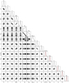 |
Fig. D.1 Correlation plot of the parameters of the planet model made with the code corner (Foreman-Mackey 2016). The marginalised posterior distribution of each parameter is represented in the diagonal and the 2D histogram contours are shown below. The red vertical lines highlight the normal prior (if any), with the dashed line being the mean value and the dotted line being the ± 1σ interval. The values of the axes are not displayed as this plot aims only at revealing parameter correlations (values are reported in Table 3). The strong linear correlation between the geometric albedo Ag and the dayside thermal flux Fday is a result of the degeneracy between reflected light and thermal emission. The plot also shows that the hotspot offset ϕthem is well defined for high Fday values, as explained in Sect. 5.1. |
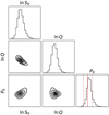 |
Fig. D.2 Same as Fig. D.1, but for the hyper-parameters of the Gaussian process used to fit the stellar activity signal. |
References
- Ahlers, J. P., Kruse, E., Colón, K. D., et al. 2020, ApJ, 888, 63 [NASA ADS] [CrossRef] [Google Scholar]
- Anderson, D. R., Temple, L. Y., Nielsen, L. D., et al. 2018, ArXiv e-prints [arXiv:1809.04897] [Google Scholar]
- Balona, L. A. 2019, MNRAS, 490, 2112 [NASA ADS] [CrossRef] [Google Scholar]
- Barnes, J. W. 2009, ApJ, 705, 683 [Google Scholar]
- Barnes, J. W., Linscott, E., & Shporer, A. 2011, ApJS, 197, 10 [NASA ADS] [CrossRef] [Google Scholar]
- Bell, T. J., & Cowan, N. B. 2018, ApJ, 857, L20 [Google Scholar]
- Benz, W., Broeg, C., Fortier, A., et al. 2021, Exp. Astron., 51, 109 [Google Scholar]
- Blackwell, D. E., & Shallis, M. J. 1977, MNRAS, 180, 177 [NASA ADS] [CrossRef] [Google Scholar]
- Bonfanti, A., Ortolani, S., Piotto, G., & Nascimbeni, V. 2015, A&A, 575, A18 [NASA ADS] [CrossRef] [EDP Sciences] [Google Scholar]
- Bonfanti, A., Ortolani, S., & Nascimbeni, V. 2016, A&A, 585, A5 [NASA ADS] [CrossRef] [EDP Sciences] [Google Scholar]
- Bonfanti, A., Delrez, L., Hooton, M. J., et al. 2021, A&A, 646, A157 [EDP Sciences] [Google Scholar]
- Borucki, W. J., Koch, D., Basri, G., et al. 2010, Science, 327, 977 [Google Scholar]
- Bourrier, V., Kitzmann, D., Kuntzer, T., et al. 2020, A&A, 637, A36 [NASA ADS] [CrossRef] [EDP Sciences] [Google Scholar]
- Charbonneau, D., Noyes, R. W., Korzennik, S. G., et al. 1999, ApJ, 522, L145 [CrossRef] [Google Scholar]
- Chazelas, B., Deline, A., Wildi, F., et al. 2019, in SPIE Conf. Ser., 11180, 111802 [NASA ADS] [Google Scholar]
- Claret, A. 2000, A&A, 359, 289 [NASA ADS] [Google Scholar]
- Claret, A. 2016, A&A, 588, A15 [NASA ADS] [CrossRef] [EDP Sciences] [Google Scholar]
- Claret, A., & Bloemen, S. 2011, A&A, 529, A75 [NASA ADS] [CrossRef] [EDP Sciences] [Google Scholar]
- Collier Cameron, A., Pollacco, D., Hellier, C., et al. 2009, in Transiting Planets, eds. F. Pont, D. Sasselov, & M. J. Holman, IAU Symp., 253, 29 [NASA ADS] [Google Scholar]
- Collier Cameron, A., Guenther, E., Smalley, B., et al. 2010, MNRAS, 407, 507 [NASA ADS] [CrossRef] [Google Scholar]
- Cowan, N. B., & Agol, E. 2011, ApJ, 729, 54 [Google Scholar]
- Deline, A., Queloz, D., Chazelas, B., et al. 2020, A&A, 635, A22 [NASA ADS] [CrossRef] [EDP Sciences] [Google Scholar]
- Dufton, P. L., Langer, N., Dunstall, P. R., et al. 2013, A&A, 550, A109 [NASA ADS] [CrossRef] [EDP Sciences] [Google Scholar]
- Dupret, M. A. 2001, A&A, 366, 166 [NASA ADS] [CrossRef] [EDP Sciences] [Google Scholar]
- Dupret, M. A., Grigahcène, A., Garrido, R., Gabriel, M., & Scuflaire, R. 2005, A&A, 435, 927 [NASA ADS] [CrossRef] [EDP Sciences] [Google Scholar]
- Ehrenreich, D., Lovis, C., Allart, R., et al. 2020, Nature, 580, 597 [Google Scholar]
- Espinoza, N., & Jordán, A. 2015, MNRAS, 450, 1879 [Google Scholar]
- Espinosa Lara, F., & Rieutord, M. 2011, A&A, 533, A43 [NASA ADS] [CrossRef] [EDP Sciences] [Google Scholar]
- Esteves, L. J., De Mooij, E. J. W., & Jayawardhana, R. 2013, ApJ, 772, 51 [NASA ADS] [CrossRef] [Google Scholar]
- Evans, T. M., Sing, D. K., Kataria, T., et al. 2017, Nature, 548, 58 [NASA ADS] [CrossRef] [Google Scholar]
- Foreman-Mackey, D. 2016, J. Open Source Soft., 24 [NASA ADS] [CrossRef] [Google Scholar]
- Foreman-Mackey, D., Hogg, D. W., Lang, D., & Goodman, J. 2013, PASP, 125, 306 [Google Scholar]
- Foreman-Mackey, D., Agol, E., Ambikasaran, S., & Angus, R. 2017, AJ, 154, 220 [Google Scholar]
- Fossati, L., Koskinen, T., Lothringer, J. D., et al. 2018, ApJ, 868, L30 [CrossRef] [Google Scholar]
- Fossati, L., Young, M. E., Shulyak, D., et al. 2021, A&A, 653, A52 [NASA ADS] [CrossRef] [EDP Sciences] [Google Scholar]
- Gaia Collaboration (Brown, A. G. A., et al.) 2021a, A&A, 649, A1 [NASA ADS] [CrossRef] [EDP Sciences] [Google Scholar]
- Gaia Collaboration (Smart, R. L., et al.) 2021b, A&A, 649, A6 [EDP Sciences] [Google Scholar]
- Gaudi, B. S., Stassun, K. G., Collins, K. A., et al. 2017, Nature, 546, 514 [NASA ADS] [Google Scholar]
- Gillon, M., Jehin, E., Magain, P., et al. 2011, in Eur. Phys. J. Web Conf., 11, 06002 [NASA ADS] [CrossRef] [EDP Sciences] [Google Scholar]
- Heng, K., Morris, B. M., & Kitzmann, D. 2021, Nat. Astron., 5, 1001 [NASA ADS] [CrossRef] [Google Scholar]
- Hooton, M. J., Hoyer, S., Kitzmann, D., et al. 2022, A&A, 658, A75 [NASA ADS] [CrossRef] [EDP Sciences] [Google Scholar]
- Hoyer, S., Guterman, P., Demangeon, O., et al. 2020, A&A, 635, A24 [NASA ADS] [CrossRef] [EDP Sciences] [Google Scholar]
- Husser, T. O., Wende-von Berg, S., Dreizler, S., et al. 2013, A&A, 553, A6 [NASA ADS] [CrossRef] [EDP Sciences] [Google Scholar]
- Jehin, E., Gillon, M., Queloz, D., et al. 2011, The Messenger, 145, 2 [NASA ADS] [Google Scholar]
- Kesseli, A. Y., & Snellen, I. A. G. 2021, ApJ, 908, L17 [Google Scholar]
- Kipping, D. M. 2013, MNRAS, 435, 2152 [Google Scholar]
- Kitzmann, D., Heng, K., Rimmer, P. B., et al. 2018, ApJ, 863, 183 [Google Scholar]
- Koch, D. G., Borucki, W., Webster, L., et al. 1998, in Space Telescopes and Instruments V, eds. P. Y. Bely, & J. B. Breckinridge, 3356, 599 [CrossRef] [Google Scholar]
- Komacek, T. D., & Showman, A. P. 2016, ApJ, 821, 16 [CrossRef] [Google Scholar]
- Kreidberg, L. 2015, PASP, 127, 1161 [Google Scholar]
- Kurucz, R. L. 1979, ApJS, 40, 1 [NASA ADS] [CrossRef] [Google Scholar]
- Lee, U., & Saio, H. 2020, MNRAS, 497, 4117 [CrossRef] [Google Scholar]
- Lendl, M., Csizmadia, S., Deline, A., et al. 2020, A&A, 643, A94 [EDP Sciences] [Google Scholar]
- Lindegren, L., Bastian, U., Biermann, M., et al. 2021, A&A, 649, A4 [EDP Sciences] [Google Scholar]
- Lomb, N. R. 1976, Ap&SS, 39, 447 [Google Scholar]
- Lothringer, J. D., Barman, T., & Koskinen, T. 2018, ApJ, 866, 27 [NASA ADS] [CrossRef] [Google Scholar]
- Maeder, A. 2009, Physics, Formation and Evolution of Rotating Stars (Springer) [Google Scholar]
- Malik, M., Grosheintz, L., Mendonça, J. M., et al. 2017, AJ, 153, 56 [Google Scholar]
- Malik, M., Kitzmann, D., Mendonça, J. M., et al. 2019, AJ, 157, 170 [Google Scholar]
- Marigo, P., Girardi, L., Bressan, A., et al. 2017, ApJ, 835, 77 [Google Scholar]
- Masuda, K. 2015, ApJ, 805, 28 [NASA ADS] [CrossRef] [Google Scholar]
- Maxted, P. F. L., Marsh, T. R., & North, R. C. 2000, MNRAS, 317, L41 [NASA ADS] [CrossRef] [Google Scholar]
- Maxted, P. F. L., Ehrenreich, D., Wilson, T. G., et al. 2021, MNRAS, in press [arXiv:2111.08828] [Google Scholar]
- Mayor, M., Pepe, F., Queloz, D., et al. 2003, The Messenger, 114, 20 [NASA ADS] [Google Scholar]
- Mazeh, T. 2008, in EAS Pub. Ser., 29, eds. M. J. Goupil, & J. P. Zahn, 1 [NASA ADS] [CrossRef] [EDP Sciences] [Google Scholar]
- Monnier, J. D., Zhao, M., Pedretti, E., et al. 2007, Science, 317, 342 [NASA ADS] [CrossRef] [Google Scholar]
- Morris, B. M., Heng, K., Jones, K., et al. 2022, A&A, in press, https://doi.org/10.1051/0004-6361/202142135 [Google Scholar]
- Parmentier, V., Line, M. R., Bean, J. L., et al. 2018, A&A, 617, A110 [NASA ADS] [CrossRef] [EDP Sciences] [Google Scholar]
- Parviainen, H. 2015, MNRAS, 450, 3233 [Google Scholar]
- Pollacco, D. L., Skillen, I., Collier Cameron, A., et al. 2006, PASP, 118, 1407 [NASA ADS] [CrossRef] [Google Scholar]
- Queloz, D., Mayor, M., Weber, L., et al. 2000, A&A, 354, 99 [NASA ADS] [Google Scholar]
- Ricker, G. R., Winn, J. N., Vanderspek, R., et al. 2015, J. Astron. Telescopes, Instrum. Syst., 1, 014003 [Google Scholar]
- Royer, F., Zorec, J., & Gómez, A. E. 2007, A&A, 463, 671 [NASA ADS] [CrossRef] [EDP Sciences] [Google Scholar]
- Scargle, J. D. 1982, ApJ, 263, 835 [Google Scholar]
- Schanche, N., Hébrard, G., Collier Cameron, A., et al. 2020, MNRAS, 499, 428 [NASA ADS] [CrossRef] [Google Scholar]
- Scuflaire, R., Théado, S., Montalbán, J., et al. 2008, Ap&SS, 316, 83 [Google Scholar]
- Skrutskie, M. F., Cutri, R. M., Stiening, R., et al. 2006, AJ, 131, 1163 [NASA ADS] [CrossRef] [Google Scholar]
- Sobolev, V. V. 1975, Light Scattering in Planetary Atmospheres, International Series of Monographs in Natural Philosophy (Pergamon Press) [Google Scholar]
- Szabó, G. M., Pál, A., Derekas, A., et al. 2012, MNRAS, 421, L122 [Google Scholar]
- Trust, O., Jurua, E., De Cat, P., & Joshi, S. 2020, MNRAS, 492, 3143 [NASA ADS] [CrossRef] [Google Scholar]
- Uytterhoeven, K., Moya, A., Grigahcène, A., et al. 2011, A&A, 534, A125 [CrossRef] [EDP Sciences] [Google Scholar]
- von Zeipel, H. 1924, MNRAS, 84, 665 [NASA ADS] [CrossRef] [Google Scholar]
- Wardenier, J. P., Parmentier, V., Lee, E. K. H., Line, M. R., & Gharib-Nezhad, E. 2021, MNRAS, 506, 1258 [NASA ADS] [CrossRef] [Google Scholar]
- Wong, I., Kitzmann, D., Shporer, A., et al. 2021, AJ, 162, 127 [NASA ADS] [CrossRef] [Google Scholar]
- Wright, E. L., Eisenhardt, P. R. M., Mainzer, A. K., et al. 2010, AJ, 140, 1868 [Google Scholar]
The plate scale of CHEOPS is 1 arcsec per pixel.
We note that there is a typo in Eq. (14) of Barnes (2009), and the terms (1 − f2) should be replaced by  .
.
All Tables
Planetary parameters obtained with the model assuming a Lambertian reflector and approximating the thermal emission as a sinusoidal function of the phase angle.
Thresholds above which a correlation between the measured flux and the background level have been detected in the eclipse observations for each of the photometric extraction method.
Model parameters for the normalisation and the systematic noise. The values reported are the one obtained for the phase-curve model with a Lambertian reflector and a sinusoid approximation of the thermal emission. All parameters had uniform priors with the sole purpose of improving convergence speed of the MCMC run.
All Figures
|
Fig. 1 Raw light curves of the four eclipses and the two phase curves measured by CHEOPS. The represented data were extracted byaperture photometry by the mission data reduction pipeline for a circular aperture radius of 25 pixels. Each data set is shifted upward with respect to the one observed before for visualisation purposes. The raw data points are shown in blue and binned once per CHEOPS orbit (black). The orange solid line is the best-fit model obtained with the modelling described in Sect. 4. The six observations are represented as a function of time since inferior conjunction according to the best-fit parameter values. |
| In the text | |
|
Fig. 2 Flux extracted with aperture photometry (DRP, aperture of 25 pixels) as a function of the image background levels for the four eclipse observations of WASP-189 b. This figure highlights the unexpected anti-correlation occurring above a given background value. The vertical dotted black line shows the threshold used to discard data points. |
| In the text | |
|
Fig. 3 Synthetic SED from the PHOENIX library (Husser et al. 2013) of a star similar to WASP-189. The stellar properties are an effective temperature Teff = 8000 K, a surface gravity logg = 4.0, and a solar metallicity. The stellar SED in blue is represented over the CHEOPS passband (330–1100 nm) shown as a black dotted line. The effective SED as seen by the CHEOPS instrument is the solid orange line, for which one can see that most of the energy lies within the 400–800 nm range and the contribution beyond 1000 nm is marginal. |
| In the text | |
|
Fig. 4 Eclipse models with and without accounting for the oblateness of the host star. The parameters used in this example are the ones reported in Lendl et al. (2020) except for the stellar rotation speed (increased by a factor of 2 to enhance the effect of rotation), the projected orbital obliquity (set to 40deg), and the orbital inclination (set to 93deg). The left panel shows the light curves normalised by the out-of-eclipse flux for the same system orientation with an oblate stellar disc (solid black line) and a spherical star (orange dashed line). On the right we show a projected view of the system during the eclipse event. The black ellipse and the orange dashed circle show the limb of the star in both cases with the same colour code. The path of the planet is represented by the straight black line and arrows, with the planet being to scale (small black disc). |
| In the text | |
|
Fig. 5 Photometric variability observed in the two WASP-189 b phase-curve time series. Top: raw flux (blue points) variations in ppm around the median value after removing outliers, de-trending for linear slope and hiding in-transit (light red shaded area) and in-eclipse (light yellow shaded area) data. Black points are raw flux variations binned once per CHEOPS orbit (98.90 min). Bottom: Lomb–Scargle periodograms of the raw flux variations shown above. The top panel represents the power spectrum of the first phase curve observed for BJD < 2 459 020, while the mid panel corresponds to the second phase-curve observation (BJD > 2 459 021). The bottom panel is the periodogram of the combined phase-curve time series. The period range covered by each periodogram goes from the Nyquist period (twice the sampling time) to the durationof the time series, and thus encompasses all detectable periodicities. The coloured triangles in the top panel mark the periods of interest. The four leftmost ones (yellow) represent the fundamental (filled triangle) and harmonic (empty triangles) frequencies of the CHEOPS orbital period. The rightmost triangle (black) and the associated vertical dashed line correspond to the orbital period of WASP-189 b. The red triangle and dashed line mark the stellar rotation period of 1.24 days computed from Lendl et al. (2020). The grey shaded area corresponds to the spectral window of the observation (spectral power induced by the sampling and the gaps of the data). |
| In the text | |
|
Fig. 6 Representation of the two possible orientations of the WASP-189 planetary system. The star is in its most probable state with the grey dashed curves marking constant stellar latitudes and with the north pole upward. In this representation, the stellar rotation causes the left and right hemispheres to appear blueshifted and redshifted, respectively. The stellar oblateness
|
| In the text | |
|
Fig. 7 Phase-folded phase curve of WASP-189 b after correction of instrumental systematics and stellar activity. This data set is obtained from a model assuming the planet is a Lambertian reflector and approximating the thermal emission with a sinusoid function. The data points de-trended from all systematics and stellar variability are shown in blue in the two upper panels. The mid-panel shows a zoomed-in view of the upper one to better visualise the phase-curve signal. The lower panel shows the residual after subtraction of the best-fit planet model. The black points represent the binned data with 100 bins per orbital period, which corresponds to a bin duration of about 40 min. The faded orange lines are 100 samples drawn from the posterior probability obtained from the MCMC run, and thus highlight the uncertainty we obtain on the best-fit model. |
| In the text | |
|
Fig. 8 Phase-folded transit light curve of WASP-189 b after correction of instrumental systematics and stellar activity. The top panel shows the normalised flux and two best-fit transit models with and without GD. The mid-panel (blue-point residuals) shows the best-fit residuals for the model accounting for GD. The bottom panel displays the residuals after removing a transit light curve without accounting for the gravity-darkened stellar photosphere. The black dashed line is the deviation of the model without GD from the model with GD. |
| In the text | |
|
Fig. 9 Heat redistribution efficiency ε as a functionof the geometric albedo Ag. The median value of ε is represented by the blue curve and the shaded areas highlight the 1 σ, 2 σ, and 3 σ uncertainty range. The value of ε is computed as the nightside-to-dayside flux ratio measured by CHEOPS. Low values of Ag indicates low reflectivity and a phase-curve amplitude mostly due to thermal emission. The thermal contribution gets smaller for higher Ag where reflected light starts to be important. |
| In the text | |
|
Fig. 10 Dayside (top) and nightside (bottom) effective temperatures of the atmosphere of WASP-189 b as a function of the Bond albedoAB and the heat redistribution efficiency ε. The lower limit of the colour scale is set to 1000 K for abetter visualisation. White dotted lines show isothermal profile across the (AB, ε) plane. The dayside and nightside temperatures are equal when ε = 1 and both go down to 0 K in the limit AB → 1. If the dayside temperature is 3000 K, then the Bond albedo values range from 0 to ~0.38, with corresponding values of the heat redistribution efficiency from ~0.59 to 0, respectively. In such a case, the maximum nightside temperature would be ~ 2250 K. |
| In the text | |
|
Fig. 11 Dayside thermal flux from WASP-189 b as a function of the Bond albedo AB and the heat redistribution efficiency ε. The flux Fday is normalised by the stellar flux F⋆. Both fluxes are computed as seen through CHEOPS passband. White dotted lines show constant flux ratios across the (AB, ε) plane. If the measured eclipse depth contains a thermal emission component with an amplitude 40 ppm, the Bond albedo may be as large as ~0.29 and as small as zero, and the corresponding heat redistribution efficiency would be zero and ~ 0.45, respectively. |
| In the text | |
|
Fig. 12 Spectral energy distribution of the planet WASP-189 b. The high-resolution synthetic SED computed with HELIOS (Malik et al. 2017, 2019) is represented in light blue and assumes the irradiating power is fully absorbed and not redistributed (AB = ε = 0). The dark blue line is the HELIOS data averaged over bins of 5 nm. The black-body profile of the maximum dayside temperature Tday, max is shown inorange. We note that accounting for emission lines in the planetary spectrum leads to a different SED with respectto the black-body approximation, with more energy in the blue end. This affects the flux measured in the CHEOPS passband (black dotted line), with the dayside of WASP-189 b appearing slightly brighter. |
| In the text | |
|
Fig. 13 Photometric variability attributed to stellar rotation as fitted by the Gaussian process. The upper panel shows in blue the time series corrected for instrumental systematics and the planet model, including transit, eclipse, and phase-curve signal. The residuals of the best-fit are represented in the lower panel (blue points). The data points binned once per CHEOPS orbit are shown in black. The faded orange lines are GP models sampled from the posterior distribution highlighting the uncertainty of the fit. The vertical dotted lines mark the time interval of the planetary transits (red) and eclipses (green). |
| In the text | |
|
Fig. B.1 Geometry used to define the angular parameters of the GD model. The x-axis points towards the observer. The z-axis is defined so that the stellar spin axis |
| In the text | |
|
Fig. D.1 Correlation plot of the parameters of the planet model made with the code corner (Foreman-Mackey 2016). The marginalised posterior distribution of each parameter is represented in the diagonal and the 2D histogram contours are shown below. The red vertical lines highlight the normal prior (if any), with the dashed line being the mean value and the dotted line being the ± 1σ interval. The values of the axes are not displayed as this plot aims only at revealing parameter correlations (values are reported in Table 3). The strong linear correlation between the geometric albedo Ag and the dayside thermal flux Fday is a result of the degeneracy between reflected light and thermal emission. The plot also shows that the hotspot offset ϕthem is well defined for high Fday values, as explained in Sect. 5.1. |
| In the text | |
|
Fig. D.2 Same as Fig. D.1, but for the hyper-parameters of the Gaussian process used to fit the stellar activity signal. |
| In the text | |
Current usage metrics show cumulative count of Article Views (full-text article views including HTML views, PDF and ePub downloads, according to the available data) and Abstracts Views on Vision4Press platform.
Data correspond to usage on the plateform after 2015. The current usage metrics is available 48-96 hours after online publication and is updated daily on week days.
Initial download of the metrics may take a while.