| Issue |
A&A
Volume 658, February 2022
|
|
|---|---|---|
| Article Number | A140 | |
| Number of page(s) | 21 | |
| Section | Interstellar and circumstellar matter | |
| DOI | https://doi.org/10.1051/0004-6361/202141477 | |
| Published online | 11 February 2022 | |
A FAST survey of H I narrow-line self-absorptions in Planck Galactic cold clumps guided by HC3N
1
Department of Astronomy, School of Physics, Peking University,
Beijing
100871,
PR China
e-mail: This email address is being protected from spambots. You need JavaScript enabled to view it.
; This email address is being protected from spambots. You need JavaScript enabled to view it.
2
Kavli Institute for Astronomy and Astrophysics, Peking University,
5 Yiheyuan Road, Haidian District,
Beijing
100871, PR China
3
Shanghai Astronomical Observatory, Chinese Academy of Sciences,
Shanghai
200030,
PR China
4
Department of Astronomy, Yunnan University,
Kunming
650091, PR China
5
Department of Physics, Anhui Normal University,
Wuhu,
Anhui
241002, PR China
6
National Astronomical Observatories, Chinese Academy of Sciences,
Beijing
100101,
PR China
7
NAOC-UKZN Computational Astrophysics Centre, University of KwaZulu-Natal,
Durban
4000, South Africa
8
Xinjiang Astronomical Observatory, Chinese Academy of Sciences,
830011
Urumqi, PR China
9
Purple Mountain Observatory, Chinese Academy of Sciences, 10 Yuanhua Road, Qixia District,
Nanjing
210033, PR China
Received:
5
June
2021
Accepted:
27
December
2021
Abstract
Using the Five-hundred-meter Aperture Spherical radio Telescope (FAST), we search for H I narrow-line self-absorption (HINSA) features in twelve Planck Galactic cold clumps (PGCCs), the starless core L1521B, and four star forming sources. Eight of the 12 PGCCs have detected emission of J = 2–1 of cyanoacetylene (HC3N). With an improved HINSA extraction method more robust for weaker and blended features with high velocity resolution, the detection rates of HINSA in PGCCs are high, at 92% overall (11/12) and 87% (7/8) among sources with HC3N J = 2–1 emissions. Combining the data of molecular spectra and Planck continuum maps, we studied the morphologies, dynamics, abundances and excitations of H I, CO and HC3N in PGCCs. The spatial distribution of HINSA is similar to that of CO, implying that HINSA features are confined to regions within and around CO emission kernels. HINSA tends to be not detected in regions associated with warm dust and background ionizing radiation, as well as regions associated with stellar objects. The L-band continnum and average background H I emission may be non-ignorable for the excitation of HINSA. The abundances of cold H I in PGCCs are approximately 3 × 10⁻⁴, and vary within a factor of ~3. The non-thermal velocity dispersions traced by C18O J = 1–0 and HINSA are consistent with each other (0.1–0.4 km s−1), larger than the typical value of HC3N (~0.1 km s−1). Carbon chain molecule (CCM) abundant PGCCs provide a good sample to study HINSA.
Key words: ISM: abundances / ISM: clouds / ISM: molecules / ISM: kinematics and dynamics / stars: formation
© ESO 2022
1 Introduction
The detection of H I with the 21 cm line (2S1∕2, F = 1–0; f0 = 1420.4058 MHz) is a milestone in the study of interstellar matter in our Galaxy (Ewen & Purcell 1951). Immediately after, astronomers tried to investigate star formations in atomic clouds, only to realize that the atomic clouds have too high a temperature and too low a density to form stars. In the 1960s, molecular clouds were identified to be the birth place of stars. Since hydrogen is the major component of molecular clouds, the syntheses of molecular hydrogen (H2) from H atoms is critical for star formation. The measurement of [H]/[H2] is very important for us to understand the chemical state of a targeted source (e.g., Cameron 1962; Gould & Salpeter 1963; Dickey et al. 1983). However, the observation of H I and H2 in molecular clouds is very difficult. H2 is a non-polarized molecule lacking permanent electric dipole moment, and thus it cannot be detected in the microwave band. Meanwhile, the crowded velocity components contributed by background and foreground emitting sources make it also hard to identify H I emission associated with any exact cloud component in the Galaxy (Li & Goldsmith 2003).
H I narrow-line self-absorption (HINSA) was demonstrated to be a good tracer of molecular clouds (Li & Goldsmith 2003, and references therein). H I self-absorption (HISA) occurs if cold atomic hydrogen is in front of a warmer emission background (e.g., Knapp 1974; Baker & Burton 1979; Wang et al. 2020). HISA is common but diverse in gas outside the solar circle. The majority of HISA features have no obvious 12CO emission counterparts (Gibson et al. 2000; Gibson 2010). Kavars et al. (2005) searched for HISA features within the Southern Galactic Plane Survey (SGPS), finding H I number densities of a few particles per cubic centimeter. The origins of HISA can be varied, including the cold neutral medium with low temperatures (15–35 K, Heiles 2001) and the “missing link” clouds in status between atomic clouds and molecular clouds (Kavars et al. 2005), as well as the cold H I component within the molecular clouds (Wilson & Minn 1977). As a special case of HISA, HINSA was defined as self-absorption feature with corresponding CO emission and line width comparable or smaller than that of CO (Li & Goldsmith 2003). The cold H I traced by HINSA has been shown to be tightly associated with molecular components. HINSA is an efficient method to detect cold H I mixed with molecular hydrogen H2. Besides CO,other molecular tracers such as OH also have central velocity tightly correlated with that of HINSA (Li & Goldsmith 2003), although no clear correlation was found for the nonthermal velocity dispersion between OH and HINSA (Tang et al. 2021).
Since it was first detected in our Galaxy, the HINSA science has been developed substantially with the observations of the Arecibo 305 m Telescope (Goldsmith & Li 2005; Krčo et al. 2008; Krčo & Goldsmith 2010; Tang et al. 2016; Zuo et al. 2018). In the optically selected nearby dark cores (Lee & Myers 1999), the volume densities of H atoms (n(H)) appear to be slightly higher than the steady-state value resultant from the competition between H I formation and destruction (Li & Goldsmith 2003). Guided by 13CO J = 1−0, the HINSA detection rate (the fraction of 13CO emitting clouds where HINSA is detected) can be as high as ~80% (Krčo et al. 2008).
The Five-hundred-meter Aperture Spherical radio Telescope (FAST; Nan et al. 2011; Li et al. 2018) located in the southwest ofChina is the most sensitive radio telescope in the L band. In the FAST era, HINSA science has a new opportunity for great advancement (Heiles 2019). Tang et al. (2020) conducted a pilot H I 21 cm spectra survey toward 17 Planck Galactic cold clumps (PGCCs) using the FAST in single-point mode. In that survey, 58% of PGCCs have detections of HINSA features, with the detection rate slightly smaller than the rates in the Taurus and Perseus regions (77%; Li & Goldsmith 2003) and molecular cores (80%; Krčo & Goldsmith 2010). This deviation may arise from limited sample and different background H I emission or reflect the different evolution statuses of these sources.
The Planck satellite (Tauber et al. 2010; Planck Collaboration I 2011) provided an all-sky survey in the submillimeter-to-millimeter range with unprecedented sensitivity. PGCCs (Planck Collaboration XXIII 2011; Planck Collaboration XVIII 2016) were released as one of the products. They are mostly cold quiescent samples but are not as dense as low-mass cores, implying that they are at very early evolution stages (Wu et al. 2012; Liu et al. 2012, 2019; Juvela et al. 2015; Zhang et al. 2020; Xu et al. 2021). The detection of HINSA features in early cold molecular clouds such as PGCCs (Tang et al. 2020) reveals the potential to improve our understanding about the transition from atomic cloud to molecular cloud.
In the present work, we observed twelve PGCCs and five comparison objects using the L-band 19-beam receiver employed on the FAST. The 19-beam receiver (Li et al. 2018) can help us quickly map the target sources. Seven of the samples are observed in the snapshot mode, which is made up of four sets of 19-beam tracking mode observations and consists of 76 pointings. We introduce the basic information of the sample in Sect. 2. The FAST H I observations are described in Sect. 3.
Another feature of this work is that the sources we observed are carefully chosen as the carbon chain molecule (CCM) abundant clouds or clumps (Sect. 2). The observed PGCCs are mainly chosen from PGCCs with HC3N emission. PGCCs with CCM production regions are chosen because they tend to contain abundant H I, since the hydrogen atom is one of the main components of hydrocarbon molecules and N-bearing CCMs (e.g., Taniguchi et al. 2016). The initial searching for carbon chain molecule (CCM) production regions began in 1970s (Turner 1971). Since then, CCMs were detected toward molecular clouds in virious environments, including the gas envelopes warmed up by young stellar objects (Suzuki et al. 1992; Sakai et al. 2008) or affected by young stellar shocks (Wu et al. 2019a,b). However, it is not clear which gas component in a PGCC is associated with the CCM production regions, the warm component accompanying young stellar objects, or the cold component embedded in the cold and dense central region. Searching for HINSA toward PGCCs could help us understand this issue. Another important reason for choosing a sample of CCM production sources is that we may have a higher detection rate of HINSA toward these sources.
Besides observations, this work also focuses on the HINSA extracting methods. The HINSA features are extracted by basically following the method of Krčo et al. (2008), denoted as “method 1” in this work. However, we point out the caveats of method 1 and give an analytic formula to quantify the requirement of high signal-to-noise (S/N) if method 1 is adopted. An improved HINSA-extracting method is proposed in this work, denoted as “method 2”. The S/N requirement for method 2 is much lower than that for method 1. Method 2 is sensitive to HINSA spectrum with high velocity resolution (thus a broad line width relative to channel width) and low S/N or HINSA features with multiple velocity components. The algorithms and the S/N thresholds of these two HINSA-extracting methods are described in Sect. 4.
Applying the improved method to the observed H I 21 cm spectra, HINSA features can be extracted in 14 of the 17 observed sources with a detection rate of 82%. The detection rate of HINSA in PGCCs is 11/12 (90%), higher than that in the sample of Tang et al. (2020). The fitting results of HINSA, HC3N J = 2–1 and CO spectra as well as the HINSA images are presented in Sect. 5. Combining the information of HINSA, HC3N, and CO emission as well as the dust continuum, the present work aims to improve knowledge of the H I abundances in PGCCs, theevolutionary statuses of PGCCs, and the excitation mechanism of HINSA in CO and CCM emission regions. In Sect. 6, we discuss the morphologies, abundances, and excitations of H I, CO, and HC3N in PGCCs. We summarize this paper in Sect. 7.
2 Sample
This work focuses on the HINSA observations toward PGCCs and the HINSA extracting methods. Besides 12 PGCCs, our sample consists of five comparison objects chosen from literature. They are also CCM abundant sources, including one starless core, L1521B, as well as four star forming sources. The star forming sources are chosen from an outflow catalog (Wu et al. 2004 and references therein).
Among the 12 PGCCs, nine have been observed in HC3N J = 2–1 using the Tian Ma radio telescope (TMRT)1, conducted as part of the survey searching for Ku-band CCM emission in PGCCs led by Yuefang Wu. The main line of HC3N J = 2–1 is F = 3–2 (18 196.3104 MHz). Eight of the 12 PGCCs have valid detections of HC3N J = 2–1.
All of the 12 PGCCs have single-point observations in J = 1–0 of CO and its isotopomers by Wu et al. (2012), using the Purple Mountain Observatory (PMO) 13.7 m telescope. Among them, 11 were mapped in these CO transitions by Wu et al. (2012). The analysis in this work focuses on PGCCs. Comparing the PGCCs and the comparison objects can lead to a clearer conclusion about the effects of the core statuses and star formation activities on the morphologies of HINSA features. The H I spectra from sources of different types can also help us to test the robustness of the HINSA extracting algorithm. However, we do not try to give any quantitative analysis about those comparison objects.
The names and coordinates of sources in our sample are listed in the first three columns of Table 1. The distribution of the sources in the Galactic plane is shown in Fig. 1. The background of Fig. 1 shows the dust temperature decomposed by Planck Collaboration XLVIII (2016) from the Planck continuum images (Planck Collaboration I 2016; Planck Collaboration XLVIII 2016)2 using the Generalized Needlet Internal Linear Combination (GNILC; Remazeilles et al. 2011) component-separation method. The PGCCs tend to be located at the margins of the emission regions of the Planck 353 μm continuum (Fig. 1).
For the twelve PGCCs in our sample, their distances were calculated using the Bayesian distance calculator3 (Reid et al. 2016) based on their coordinates and velocities. The Bayesian calculator constrains the probability density function (PDF) of distance based on four types of information: kinematic distance (KD), the spiral arm model (SA), Galactic latitude (GL), and parallax source (PS). The velocity dispersion has been taken into account to give the uncertainty of kinematic distance. Their angular size (Ddust) and dust temperatures (TECC) can be quoted from the Planck early cold core (ECC) catalog (Planck Collaboration XXIII 2011), which is the pioneer sample of PGCCs. For the other five sources, their distances are adopted from literature (see Table 1). Their Ddust can also be obtained if the Hershcel continuum data are available. The distance, Ddust, and TECC are listed in the fourth to sixth columns of Table 1.
Sources.
3 Observation and archive data
3.1 H I observations using the FAST
The FAST4 is a ground-based radio telescope built in the Guizhou province of southwest China (Nan et al. 2011), and it is the most sensitive single-dish telescope. The tracking accuracy is about 0.2′ (Jiang et al. 2019). For zenith angle θZA < 26.4°, the illuminated aperture is 300 meters. A 19-beam receiver in the L band is employed. The full width at half maximum (FWHM) beam size is about 3′ around 1420 GHz for θZA < 26.4°, which is about half of the angular spacing between two neighboring beams, 5.87′. Our observations(2019a-020-S) were conducted on August 5 and 11, 2019. The on-source time was ten minutes for each source. Our targets all have θZA smaller than 20° during the observations, as listed in Table 1. It takes approximately ten minutes or less to change the targeted sources. The spectral mode with 1024 k channels evenly spaced between 1 and 1.5 GHz was adopted for our observations, corresponding to a channel spacing of ~0.1 km s−1 for H I linewith a rest frequency of ~1420 GHz.
Seven ofour sources were observed using the tracking mode with the central beam (beam 1) always pointing on the center of the target, while the other ten sources were observed with the snapshot mode (see Table 1). The snapshot mode is made up of four sets of tracking mode observations. In snapshot mode, the targeted locations of the central beams between two successive tracking mode observations are slightly shifted (see Fig. 2). The map obtained in snapshot mode is spatially half-Nyquist sampled.
The power spectra are recorded at every 0.1 s. For calibration, a high-level noise (10 K) was injected lasting one second for every two seconds. The system temperature is about 20 K for θZA < 20°. For a point source, the beam efficiency is constant, with a value of ~0.6 for θZA < 26.4°. It will decrease to ~0.5 if θZA increases to about 36° (Jiang et al. 2019). For an extended source, the beam efficiency should be adopted as 0.85, instead. Figure 3 shows the comparison between the H I 21 cm spectrum of G173.3-16A1 obtained by the FAST and that from the Effelsberg-Bonn HI Survey (EBHIS; Winkel et al. 2016). They are consistent with each other if a beam efficiency of 0.85 is adopted for the FAST observation.
Binned with a channel spacing 0.1 km s−1, the H I 21 cm spectra we obtained have rms noises of 30–40 mK for sources observed in the tracking mode and 60–80 mK for sources observed in the snapshot mode.
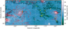 |
Fig. 1 Galactic longitude-latitude positions of the 17 sources in our sample. Yellow and cyan hexagons represent the 12 PGCCs and the other five sources, respectively. The size of the hexagon represents the covering area of the 19-beam receiver of the FAST. The dot within each hexagon shows targeted locations of the central beam (Beam 1; Fig. 2). The background image shows Planck dust temperature distribution. The black contours with levels of 3, 7, and 11 Myr sr−1 represent the Planck 850 μm continuum. The red contours represent the Hα emission (Finkbeiner 2003) in units of R (106∕4π photons cm−2 s−1 sr−1), with levels from 15 to 215 stepped by 40. |
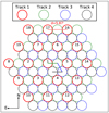 |
Fig. 2 Configuration of the 19-beam receiver of FAST (Li et al. 2018). Each snapshot mode observation consists of four single-point-mode observations. Equatorial coordinate system is adopted for the tracking mode, while Galactic coordinate system is adopted for the snapshot mode. |
3.2 HC3N J = 2–1 observations of nine PGCCs
Among the 12 PGCCs, nine were observed in HC3N J = 2–1 using the Tian Ma radio telescope (TMRT). Observations were conducted in July of 2017 and August of 2018.
The TMRT is a 65-m diameter fully steerable radio telescope located in Shanghai (Li et al. 2016). The pointing accuracy is better than 10′′. The main-beam efficiency is 0.60 in the Ku band from 12 to 18 GHz (Wang et al. 2015). The front end is a cryogenically cooled receiver covering a frequency range of 11.5–18.5 GHz. The digital back-end system (DIBAS Bussa & VEGAS Development Team 2012) is employed, which supports a variety of observing modes for molecular line observations. Mode 22 was adopted for our observation.In this mode, each of the three banks (Bank A, Bank B, and Bank C) has eight subbands with a bandwidth of 23.4 MHz and 16384 channels. The center frequency of each subband is tunable to an accuracy of 10 kHz. The calibration uncertainty is 3% (Wang et al. 2015). The Ku band observations cover the transition of HC3N J = 2–1 (18.196226 GHz). The velocity resolution is 0.023 km s−1 near 18 GHz.
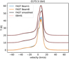 |
Fig. 3 Blue and orange solid line are the H I 21 cm spectra obtained by the FAST beam 1 and beam 8, respectively. The spectra werecalibrated adopting a beam efficiency of 0.85 for extended source. The red dotted lines are the spectra from the EBHIS (Winkel et al. 2016). The black solid lines are the FAST H I 21 cm spectra smoothed to have a velocity resolution similar to that of the EBHIS spectrum. To avoid overlapping, the red dotted lines and the black solid lines have been moved up by 10 and 20 K for beam 1 and beam 8, respectively. |
3.3 Archive data of CO and dense gas tracers
The spectral of the J = 1 − 0 transitions of 12CO as well as its isotopomers 13CO and C18O were extracted from Wu et al. (2012). Following up the releasing of PGCCs, Wu et al. (2012) observed the three CO lines towards 673 PGCCs using the PMO 13.7 m telescope5. The morphologies and dynamic properties of PGCCs are well understood thanks to the CO mapping observations (Wu et al. 2012; Liu et al. 2012, 2013; Meng et al. 2013; Zhang et al. 2016, 2020). All 12 PGCCs have single-point observations of these three CO lines. Among them, all except for G174.08-13.2 have been mapped in these lines. The CO spectra can help to identify HINSA by providing us the initial guesses of the velocity and line width of the HINSA feature (see Sects. 4 and 5.2).
Observations of emission lines of dense gas tracers toward PGCCs are rare. Among the sources in this work, two PGCCs, G165.6-09A1 and G174.4-15A1, have been mapped in C2H N = 1–0 (87.316925 GHz) and N2H+ J = 1–0 (93.173397 GHz) using the PMO 13.7 m telescope (Liu et al. 2019). The G192.2-11A2 has been mapped in HCO+ J = 1–0 (89.188523 GHz) using the Instituto de Radioastronomía Milimétrica (IRAM) 30 m telescope6 (project ID: Delta03-13). The observation of HCO+ J = 1−0 in G192.2-11A2 was conducted on May 3 of 2014, with a velocity resolution of 0.16 km s−1.
4 Methods of extracting HINSA
The H I 21 cm spectrum toward a molecular cloud is a mixture of foreground and background emission and absorption features originated from cold H I component in that molecular cloud. It is not easy to extract the absorption components from an H I 21 cm spectrum, since the shape of the spectrum without absorption features (TH i) is unknown. A reference point with the same foreground and background H I emission with the target source but showing no absorption features is difficult to find.
Combining Eqs. (1) and (5) from Li & Goldsmith (2003), the observed continuum-subtracted H I spectrum brightness temperature along the HINSA sight line is
![Mathematical equation: \begin{equation*} \begin{aligned} T_{\textrm{r}} =\;& [T_{\textrm{c}}e^{-\tau_{\textrm{b}}}+T_{\textrm{b}}(1-e^{-\tau_{\textrm{b}}})]e^{-\tau}e^{-\tau_{\textrm{f}}} \\ & + T_{\textrm{ex}}(1-e^{-\tau})e^{-\tau_{\textrm{f}}}+T_{\textrm{f}}(1-e^{-\tau_{\textrm{f}}}) - T_{\textrm{c}}. \end{aligned} \end{equation*}](/articles/aa/full_html/2022/02/aa41477-21/aa41477-21-eq1.png) (1)
(1)
Here, τ is the optical depth of the cold HI component τb = p(τf + τb), τf and τb denote the foreground and background H I optical depths, and Tc is the continuum brightness temperature. Tex, Tb, and Tf are the excitation temperatures of the cold H I component, the background warm H I component and the foreground warm H I component, respectively. TH I can then be expressed asTr|τ=0.
If Tf = Tb and both τf ≪ 1 and τb ≪ 1, the absorbed component of H I spectrum can be expressed as in Eq. (8) of Li & Goldsmith (2003):
 .\end{equation*}](/articles/aa/full_html/2022/02/aa41477-21/aa41477-21-eq2.png) (2)
(2)
Equation (2) leads to the expression of TH I as
 (3)
(3)
To avoid overfitting, parameters p, Tex, τf, and Tc should be known parameters or fixed as reasonable values.
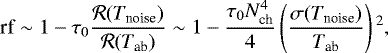
The excitation temperature (Tex) of HINSA is assumed to be the value of molecular gas ~10 K, which is much smaller than Tr. Tc should be smaller thanTex and Tr, if it is adopted as the typical value of the L-band intensity of the Galactic background emission ~ 3.5 K (Li & Goldsmith 2003). We extracted the L-band background continuum intensities for our sources from the Bonn-Stockert survey (Reich 1982; Reich & Reich 1986), which gives a mean value of 3.9 K with a standard deviation of 0.2 K. Neglecting Tc is reasonable and may lead to an overestimation of the optical depth of HINSA by ~10%.
Each of our sources has a short distance d compared with the galactics scale. Because of the short distance and low Galactic latitude b (Table 1), the height from the Galactic plane dsin(b) is small compared with the scale height of the Galactic H I layer (~350 pc; Lockman 1984; Nakanishi & Sofue 2003). Most of the H I emitters along the line of sight should be located behind the absorption source. We believe that p should be close to 1 for most of our targets, and we adopt p = 1 hereafter. We note that, if p < 1, this assumption may lead to underestimations of the HINSA optical depth and column density. In the optical thin limit, the obtained optical depth of HINSA would be approximately pτreal, where τreal is the real optical depth.
If p = 1, τf = 0, and Tex and Tc are ignored, Eq. (3) can be simplified as

Despite its simple form, Eq. (5) does not deviate much from Eq. (3) for HINSA, which has low optical depth.
The key step in extracting HINSA is to make reasonable estimations of the optical depths of cold H I (τ) in Eqs. (3) or (5), and to obtain the corresponding TH I with the highest probability to represent the real unabsorbed spectrum. The HINSA extracting methods (method 1 and method 2) described below are optimized for HINSA with Tex ≪ Tr and Tc ≪ Tr. Equation (5) helps to estimate the S/N requirement of method 1 and shed light on the motivation of method 2. Great care is required if these methods are implemented to extract absorption features of HISA clouds with warmer gas, significant foreground HI emission, or significant background continuum emission.
4.1 Method 1
HINSA usually shows significant features in the second derivative representation of Tr (Krčo et al. 2008). It is assumed the τ can be expressed as (multi-)Gaussian function:
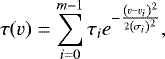 (6)
(6)
where τi, σi, and vi represent the optical depth, velocity dispersion, and central velocity of the ith component, respectively. Free parameters (τi, σi, vi) are requiredto be fit during the extraction of HINSA features. The initial trial values of (τi, σi, vi) and the fixed parameter Tex can be estimated from emission lines of other species, especially those supposed to have space distributions similar to the cold H I in molecular cloud.
The Gaussian fitting tries to obtain a smooth curve, which can be expressed as a straight line or other analytic function. However, the TH I is unknown and cannot be assumed as a linear function of velocity or frequency. Thus, the Gaussian fitting cannot be directly applied to extract HINSA. Instead, the fitting process can be conducted under a relaxed judgment of the fit curve (TH I); that is, TH I should look smoothest.
TH I can be obtained through minimizing the sum of the square of second derivative of Tr, denoted as  in this work. This method (method 1) was first highlighted by Krčo et al. (2008) to extract HINSA. Here,
  is expressed as
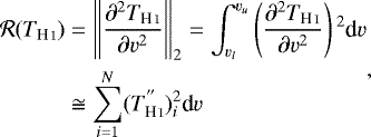 (7)
(7)
where vu –vl is the frequency or velocity range that we are interested in. The  in Eq. (7) represents the numerical version of the second derivative of TH I:
 (8)
(8)
where Δch is the channel spacing of the spectrum.
The basic idea of this method is to find a set of parameters (τi, σi, vi) that will reasonably fill the dips of Tr through Eq. (3). The TH I with minimal  value is the smoothest TH I that can represent the unabsorbed spectrum.
However, this method (also denoted method 1) has theoretical defects and is noise sensitive. We give an analytic formula to quantify the S/N threshold of method 1 in Sect. 4.1. An improved method (method 2) is proposed and described in Sect. 4.2.
4.1.1 Shortcomings of method 1
TH I usually shows a complex profile. To estimate the S/N of the HINSA detection in the second derivative representation ( ), TH I is approximated by a Gaussian function with a line width of Δw and a peak intensity of Tpeak. Here, Tpeak and Δw = NchΔch are adopted as the typical height and typical width of TH I, respectively. S/N
 can then be estimated from Eq. (8), and the second derivative of a Gaussian function (e.g., Eq. (2) of Krčo et al. 2008), and expressed as
 (9)
(9)
The  term requires a very high S/N of the spectrum. Another problem is that, when Tr is multiplied by a factor of g during the fitting process, the noise will also be amplified by the same factor. The value of this amplification factor g can be estimated from Eq. (5) as
 (10)
(10)
In theory, the original TH I will not be fully recovered through this method, since the  value contributed by the noise will also be amplified. The deviation between the original TH I and the fit TH I is systematic, and it can be reduced but never completely eliminated by an improving S/N.
4.1.2 S/N threshold of method 1
Here, we further explain why method 1 can only partly extract the HINSA feature especially when S/N is low, and we try to quantitatively assess the performances of method 1 when applied to spectra with different S/Ns. We considered that there is a linear spectrum that has an absorption feature with a Gaussian-like optical depth:
 (11)
(11)
The  value corresponding to a test value of τ0 (denoted as τ0,t) can be expressed as
 (12)
(12)
The fit value of τ0 (denoted as τ0,f) can be obtained by solving the following equation:
 (13)
(13)
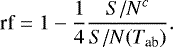
Here, we assume that τ0,f is small and thus e2τ0,f ~ 1. A recovering factor (rf) is defined as
 (14)
(14)
which represents the proportion of the HINSA extracted through method 1. Equation (13) leads to
 (15)
(15)
where σ(Tnoise) is the rms of the noise. The S/N threshold for method 1 (S/Nc) is defined as the value of Tab∕σ(Tnoise) when rf = 3∕4, which leads to
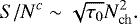 (16)
(16)
The recovering factor can then be expressed as
 (17)
(17)
If S/N(Tab) is smaller than S/Nc, rf should be small, and Eq. (17) is only statistically valid. Thus, it is not permitted to obtain the optical depth of HINSA through dividing the fit value by rf. In such a case, method 1 either can only partly extract the HINSA feature or totally fails.
Taking the channel spacing of our spectra Δch as 0.1 km s−1, the absorption line width as 1 km s−1 (corresponding to Nch = 10), and τ = 0.1, Eq. (16) leads to S∕Nc > 30. Keep in mind that S∕Nc is defined on Tab scale, and it will be multiplied by a factor of ten if defined on a Tr scale. Such a high S/N cannot always be achieved in observations.
4.2 Method 2
The main difficulty of method 1 is that it recovers TH I by multiplying Tr by a factor of ~eτ, which leads to the multiplication of noise simultaneously. To inhibit the increasing of noise, we replace the multiplication on Tr in Eq. (5) (or Eq. (4)) by an addition operation. After a simple manipulation, Eq. (5) can be rewritten as
 (18)
(18)
where  means the fit TH I. This equation highlights the possibility of keeping the noise component in TH I constant during the fitting process and equal to that in Tr if the TH I term on the right side is replaced by its smoothed version TH I,smooth. It is reasonable since we expect that TH I is smooth and can be approached by low-order polynomial.
More specifically, the fitting process of method 2 consists of five steps, including
- 1.
Calculating TH I through Eq. (3) for each given test value of free parameters.
- 2.
Obtaining THI,smooth, a smooth version of TH I; for example, by nth-order polynomial fitting.
- 3.
Updating TH I using Eq. (18).
- 4.
Calculating the
 value.
 - 5.
Repeating the above steps to find the minimal
 value and its corresponding TH I.
4.2.1 Advantage of method 2
Since most of our HINSA features are weak, it is safe to assume that τ0 ≪ 1, which would produce a near-Gaussian absorption dip. Method 2 is to recover TH I by adding a smoothed near-Gaussian component to Tr. It splits the multiplying term eτTHI in Eq. (5) into two terms: one keeps the noise and details, the other is smoothed. What we try to do is to balance the resolution and S/N. In method 2, the noise will not increase much, and the velocity resolution is kept since the smoothing is not conducted on Tr, but on TH I which is expected to be smooth. In this work, we used polynomial fitting to obtain a smooth version of  , but other methods such as convolution could also be used.
Once  is obtained, the absorbed component can be calculated through
 (19)
(19)
where  represents the fit TH I, and Tab should be apositive quantity. If the HINSA is optically thin, the noise intensity of Tab given by method 1 would be small with a value of approximately τTnoise. If method 2 is adopted, the calculated Tab should look even smoother since the amplification of noise in
  has been restrained.
4.2.2 S/N threshold of method 2
We now quantitatively assess the performance of method 2 and compare it with method 1. Method 2 works when
 (20)
(20)
which leads to
 (21)
(21)
Here, δ(X) represents the standard deviation of X. It is importantto note that Tab is a fit curvethat does not contain noise. If Eq. (21) is satisfied, we say that the absorption feature against the noise has a significance level higher than five sigma when extracted using method 2. Equation (21) can be satisfied when S/N(Tab) is higher than the S/N threshold for method 2, denoted as S/Nc;n. To derive S/Nc;n from Eq. (21), we used
 (22)
(22)
and the approximation
 (23)
(23)
Equation (21) can then be approximated as
 (24)
(24)
which leads to
 (25)
(25)
From Eq. (25), we can say that method 2 is analogous to the Gaussian fitting, since both of them have sensitivities proportional to the square root of the line widths. In contrast to method 1, method 2 favors extracting features with relatively large line widths resulting from multiple absorption components or high velocity resolution. The S/Ns of the spectra required by method 2 are much smaller than those by method 1.
4.3 Comparison between method 1 and method 2
Method 2 is an updated version of method 1. It overcomes the downsides of method 1 by introducing a intermediate step of smoothing, and thus has less strict requirement on S/N. If the TH I spectral structure is too complex, method 2 may lose resolution.
If the absorption dip deviates from Gaussian shape, the fit unabsorbed spectrum ( ) may be larger or smaller thanthe real TH I. For method 1, the fit
  tends to be smaller than TH I, because a solution of
  larger than TH I will be more severely penalized by the amplification of noise. For method 2, the fit
  has no system bias of being larger or smaller than the real value. Thus, method 2 is less predictable, and method 1 seems to be more robust when the absorption dip deviates much from Gaussian shape. However, the results of the two methods in such cases are both somewhat unreliable.
In practice, method 1 is applicable only when S/N > S/Nc (Sect. 5.2). It confirms the validity of the threshold of the S/N (S/Nc) defined in Eq. (16), which describes the requirement of method 1. It also highlights the usefulness of method 2. For molecular clouds such as PGCCs, S/N ~S/Nc requires a FAST on-source integration time of ~10 min, where the S/N is that of the absorption feature in the observed H I spectrum. For FAST drift-mode observations (Li et al. 2018), the effective integration time is ~40 s (Zhang et al. 2019). Method 2 provides a possibility to extract HINSA features from spectra with such short integration time.
5 Result
5.1 CO parameters
Among the 12 PGCCs in our sample, all except for G174.08-13.2 have been mapped by Wu et al. (2012) in J = 1–0 of 12CO and its isotopomers (Sect. 3.3). To match the H I 21 cm spectra, the J = 1–0 spectra of 12CO and its isotopomers of the 11 mapped PGCCs were smoothed to have an angular resolution of 3 arcmin. Figure 4 shows the CO spectra extracted from the locations of the central beam of the H I observations. Those spectra are fit to obtain line parameters, which can help us to extract HINSA features from the H I 21 cm spectra (Sect. 5.2). For G174.08-13.2, the CO parameters derived from its single-point observations by Wu et al. (2012) are adopted.
Assuming 12CO J =1−0 is optically thick (τ ≫ 1) and the beam filling factor is a unit, the excitation temperature can be expressed as (Kwok 2007)
![Mathematical equation: \begin{equation*}T_{\textrm{ex}} = \frac{h\nu}{k}/\ln\left\{1 + \left[ \frac{k}{h\nu} \left(T_{\textrm{CO}}^{\textrm{peak}}+J(T_{\textrm{bg}})\right) \right]^{-1} \right\} ,\end{equation*}](/articles/aa/full_html/2022/02/aa41477-21/aa41477-21-eq45.png) (26)
(26)
where  is the peak brightness temperature of 12CO J = 1–0, the background temperature (Tbg) can be adopted as 2.73 K, and
 (27)
(27)
Among the 11 sources observed by Wu et al. (2012), nine have single-peak spectra of 13CO J = 1–0. We fit them with a single Gaussian profile. The other three sources, G170.88-10.92, G172.8-14A1, and G174.4-15A1, have double-peak spectra of 13CO J = 1–0, and fittings of double Gaussian profiles are applied. Gaussian fitting is also applied to the spectra of 12CO J = 1–0 and C18O J = 1–0, with the number of velocity components same as that of 13CO J = 1–0.
The column densities of 13CO and C18O are calculated following the method described in Wu et al. (2012). Adopting the typical abundance ratios X[H2]/X[13CO] = 89 × 104 (McCutcheon et al. 1980; Pineda et al. 2013) and X[H2]/X[C18O] = 7 × 10⁶ (Frerking et al. 1982), the H2 column densities  (H2) and
  (H2) can be calculated. The peak brightness temperatures of 12CO J = 1–0, the Gaussian parameters of 13CO J = 1–0 and C18O J = 1–0, and the gas column densities derived form the CO emission are listed in Table 2.
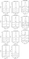 |
Fig. 4 Spectra of J = 1–0 of 12CO, C13O, and C18O (Wu et al. 2012) are shown from top to bottom in each panel. |
5.2 Extracting HINSA
Both method 1 and method 2 are applied to extract HINSA features in our spectra. The free parameters to be fit are τi, vi, and σi with i = 0, 1,..., m − 1 (Sect. 4), and m is the number of velocity components determined from CO emission or quoted from literature. For all sources, τi is initially set as 0.1. Tex is fixed as 10 K, and it will only introduce a small value of uncertainty (Sect. 5.2.4).
For PGCCs, initially, vi is adopted as the central velocity of 13CO J = 1–0 (Table 2), and σi is adopted as
 (28)
(28)
Here, the ΔV represents the FWHM of the spectral line, and the correction for the different molecular weight between 13CO and H I has been conducted.
For comparison objects, the initial guesses of central velocities are adopted as the system velocities quoted from literature. The system velocities are 6.6 km s−1 for L1489 (Wu et al. 2019a), 6.4 km s−1 for L1521B (Hirota et al. 2004), 9.0 km s−1 for IRAS 05413-0104 (Zhang et al. 2021), 10.0 km s−1 for HH25 MMS (Gibb & Davis 1997; Wu et al. 2004), and 0.5 km s−1 for CB34 (Codella & Scappini 2003). The initial values of line widths are set as 1 km s−1. We used the L-BFGS-B algorithm implemented by the Python package Scipy7 to minimize  and obtain corresponding fit parameters.
5.2.1 Performances of method 2 toward individual objects
The fitting results of G174.4-15A1 are shown in Fig. 5 as examples to present the different performances of the two methods. For G174.4-15A1, there are two gas components with velocities traced by CO emission close to each other (Table 2). Method 1 can partly extract HINSA corresponding to the bluer velocity component (VLSR ~ 5 km s−1), but it fails to extract HINSA corresponding to the redder velocity component (VLSR ~ 6.8 km s−1). This result is expected by Eq. (16). For the bluer component, S/N(Tab) is similar to S/Nc. However, for the redder component, S/N(Tab) is smaller than S/Nc (see Table 3). If method 2 is adopted, both of the two HINSA features can be extracted. This example confirms that method 2 can extract absorption features from H I spectra with low S/N and blended absorption components.
To test the robustness of method 2, we also compared the fitting result of the two methods toward the spectra of G170.88-10.92. The H I spectrum of G170.88-10.92 shows a single dip with a high S/N. The fit results of the two methods are very close to each other (see Fig. 6). For the center beam, the optical depths fit by the two methods have a deviation of less than 10 percent. The performances of the two methods are similar to each other when the S/N is high. The fitting result of method 2 should be reliable. This is confirmed by the similarity between the distributions of CO emission lines and H I absorption features for both G174.4-15A1 and G170.88-10.92 (see Sect. 5.2.3).
CO parameters.
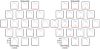 |
Fig. 5 HINSA features of G174.4-15A1 extracted by method 1 (left) and method 2 (right). Method 1 fails to fit the HINSA component because of the low S/N and the blending of two absorption components with similar velocities. In each panel, the gray line is the observed spectrum Tr, the blue line is the recovered TH I, and the red line is Tab. The Tab shown here has been multiplied by a factor of five. |
5.2.2 Performances of method 2 toward central beams
Method 2 was adopted to obtain the HINSA parameters for all the H I 21 cm spectra. For each source, the observed spectrum of the central beam (beam 1) as well as the extracted HINSA are shown in Fig. 7. Among the 12 PGCCs, ten have HINSA features on the central beam spectra that can be successfully extracted using method 2. The exceptions are G160.51-17.07 and G165.6-09A1. It corresponds to a HINSA detection rate of 83%.
The fit parameters of HINSA, including the optical depth, central velocity, line width of HINSA and the height of the absorption dip (Tab) are listed in Table 3. S/N(Tab), defined as the ratio between the peak intensity of Tab fit through method 2 and the noise intensity Tnoise, is also listedin Table 3.
For a central beam spectrum that can be successfully fit using method 2, the S/N threshold of method 1 (S/Nc) is calculated through Eq. (16). To obtain S/Nc, the values ofτ0 and ΔV fit through method 2 are used, and Nch is adopted as ΔV∕Δch. Most of our spectra have S/N(Tab) comparable to or even larger than S/Nc. The sources whose HINSA features can be partly extracted using method 1 are labeled in Table 3. From Fig. 8, it is clear that spectra with successful fittings by method 1 all have S/N(Tab) > S/Nc. This impliesthat the S/N threshold of method 1 given by Eq. (16) is reasonable, and it is essential to apply method 2 to extract HINSA features from the H I spectra of this present work.
If method 1 is applied, HINSA features can only be extracted in seven PGCCs (Table 3), corresponding to an extracting rate of 58%. This value is similar to the value of Tang et al. (2020) but lower than the HINSA detection rate of method 2.
HINSA parameters fit using method 2.
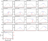 |
Fig. 7 H I 21 cm spectra at the center beam. In each panel, the gray line is the observed spectrum Tr, the blue line is the recovered TH I using method 2, and the red line is Tab. Values of Tab on the y-axis range from 0 to 20 K for all sources except G174.08-13.2, which uses 0–60 K. The orange and blue squares represent the sources that can and cannot be successfully fit using method 1. The blue line is not shown for spectrum with fit τ smaller than 0.01. |
5.2.3 HINSA maps
The maps of the integrated intensity of the optical depth of HINSA features extracted by method 2 are overlaid by the contours of CO emission. The sources observed in snapshot mode and tracking mode are shown in Figs. 9 and 10, respectively. Comparing the emission regions of HINSA and molecular lines can help us to confirm the detections of HINSA. It can also help us to study the correlation between the distribution of cold H I and other species.
We find that HINSA features can be extracted in the north-west margin of the map of G165.6-09A1. This makes G160.51-17.07 the only observed PGCC that does not show any HINSA feature. The detection rate of HINSA features in PGCCs could be as high as 11/12 (~90%) using method 2 if H I spectral of all beams are taken into consideration.
Among five comparison objects, only L1251B, HH25 MMS, and CB34 have HINSA features, with a detection rate lower than the value in PGCCs. The morphologies and environments of HINSA in PGCCs and comparison objects are further discussed in Sect. 6.2.
5.2.4 Uncertainties of HINSA parameters
The Tex of CO is close to 10 K (Sect. 6.1). The TECC of all sources except G165.6-09A1 have values of about 10 ± 2 K. Thus, it is reasonable to adopt the excitation temperature of HINSA as 10 K (Sect. 5.2). For Tr ~ 50 K and a uncertainty of excitation temperature σ(Tex) = 2 K, the relative error of the fit optical depth can be estimated as
 (29)
(29)
which is comparable with the values transferred from the data errors (Table 3).
It is important to note that the H I column density traced by HINSA is the value for cold H I mixed within a molecular cloud. If there is no background emission with TH I > Tex, there will be no HINSA, and this may lead to the underestimations of the column density of cold H I and the detection rate of HINSA.
Although method 2 can significantly reduce the requirement for a S/N, the HINSA features may still be difficult to extract if TH I is too complex. If the value of the fit optical depth is too low, it would not be easy to judge if the extracted absorption feature is a real HINSA signal. The lower limit of τ to be safely extracted is discussed in Sect. 5.2.5.
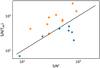 |
Fig. 8 Distribution of S/Nc and S/N(Tab) for the H I spectra of the central beams (Table 3). Here, S/N(Tab) is the ratio between the intensity of absorption dip revealed by method 2 and the spectra noise, and S/Nc is the signal-to-noise threshold required by method 1 (Sect. 5.2.2). The orange and blue squares represent the sources that can and cannot be successfully fit using method 1, respectively. The black line represents x = y. As predicted, the black line is the separation line between the two cases. |
5.2.5 Lower limit of τ to be safely extracted
Assuming both TH I and Tab have Gaussian shapes with their central velocities aligned, and their line widths are 10 and 1 km s−1, respectively, Tr will only have a dip-like structure when
 (30)
(30)
which leads to
 (31)
(31)
Only HINSA with τ larger than 0.01 can be safely extracted. If the fit optical depth τ0,f has value smaller than 0.01, the fitting results should be considered as unreliable. In such case, the fit absorption feature may be a misleading signal introduced by the irregularity of the background H I emission. If the fit optical depth is smaller than or equal to 0.01, it would be listed in Table 3 as 0.01, which means that the fitting result is not reliable.
HC3N J = 2–1 parameters.
5.2.6 Column density of H I traced by HINSA
The column density of H I can be calculated through (Li & Goldsmith 2003)
 (32)
(32)
The total gas column densities (N(H2)) are adopted as the values derived from CO spectra (Sect. 5.1) to calculate the abundances of cold H I.
The values of column densities and abundances of H I are also listed in Table 3. We provide discussions concerning the H I abundances of PGCCs in Sect. 6.3.
5.3 HC3N
Nine PGCCs have been observed in HC3N J = 2–1 using the TMRT 65-m telescope (Sect. 3.2). To compare the intensities and line widths of HINSA and HC3N in PGCCs, the spectra of HC3N J = 2–1 are shown in Fig. 11. The 1sigma noise levels are about 45 mK when the spectra are binned to have a channel width of ~0.05 km s−1. All of those PGCCs, except for G178.98-06.7, have a valid detection of HC3N J = 2–1. Although the CO spectra of several PGCCs such as G159.2-20A1, G172.8-14A1, and G174.4-15A1 have double velocity components with separations of ~1 km s−1, all of the detected HC3N J = 2–1 spectra show single velocity components.
The HC3N J = 2–1 spectra are fit using the hyperfine structure (HFS) fitting procedure provided by Gildas/CLASS8. If the fit optical depth of the spectrum tends to be smaller than 0.1, the fitting procedure will give a fitting result with optical depth adopted as 0.1. The fit parameters include the peak intensity (Tpeak), central velocity (VLSR), line width (ΔV), and the optical depth (τ) of the main line of HC3N J = 2–1. These parameters are listed in Table 4.
G174.06-15A1 and G174.08-13.2 have peak brightness temperature of HC3N J = 2–1 larger than 1 K. Their optical depths are 0.4 ± 0.1 and 0.5 ± 0.1, respectively. Assuming that the beam filling factor f is unit and the background temperature Tbg = 2.73 K, the excitation temperatures of HC3N J = 2–1 would be derived as 6.4 K and 7.7 K for G174.06-15A1 and G174.08-13.2, respectively. For G165.6-09A1 and G172.8-14A1, the fit optical depths are larger than 1. The reason may be that the S/Ns are not high enough for these two sources. The HC3N J = 2–1 of G159.2-20A1, G173.3-16A1 and G174.08-13.2 are optically thin with optical depths smaller than 0.1.
Under local thermodynamic equilibrium (LTE) assumption, the equation to calculate the molecular column density is (Garden et al. 1991; Mangum & Shirley 2015)
 (33)
(33)
where B, μ, and Q are the rotational constant, the permanent dipole moment, and the partition function, respectively. These transition parameters can be obtained from “Splatalogue9”. The beaming factors may be much smaller than one for most sources, except for G174.06-15A1 and G174.08-13.2. The excitation temperatures are adopted as 5 K to calculate the beam-averaged column densities of HC3N. The column densities of HC3N are also listed in Table 4. For G165.6-09A1 and G172.8-14A1, if the excitation temperature given by HFS fittings is adopted, the value of the calculated column densities will only change by less than 5 percent. The average abundance of HC3N is 2.2 × 10⁻⁹ with a standard error of 0.8 × 10⁻⁹.
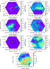 |
Fig. 9 Backgrounds: strengths of HINSA measured in the snapshot mode, extracted using method 2. Black contours: 13CO J = 1–0 emissions, which have been smoothed to the angular resolution of H I observations. Big black boxes: areas covered by CO data. Blue crosses: sampled points of the FAST, and red circle: center beam. Small red boxes and triangles: Class I/II and Class III YSOs. In panels a and c, the white contours represent the emission of C2H N = 1–0 within the white rectangles (Liu et al. 2019). In panel f, the small black rectangle represents the mapped region of the IRAM HCO+ J = 1–0 and C18O J = 2–1 observations, which are shown in Fig. 14. |
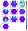 |
Fig. 10 Backgrounds: strengths of HINSA measured in the tracking mode. Symbols have the same meanings with those in Fig. 9. |
6 Discussions
6.1 CO and dust emission
The left panel of Fig. 12 shows the correlation between the H2 gas column densities derived from 13CO (N13CO(H2)) and C18O ( (H2)). N13CO(H2) and NC18O(H2) are consistent with each other within a factor of 3. For sources with low column densities (
 (H2) < 1022), the gas column densities derived from C18O tend to be smaller than those derived from 13CO. This may result from the low S/Ns for C18O J = 1–0 when the gas column densities are small. Another explanation is that C18O is more easily photo-dissociated by the external radiation field compared with 13CO, especially for sources with low column density and extinction, such as PGCCs (Shimajiri et al. 2014; Schultheis et al. 2014; Shetty et al. 2011).
Planck Collaboration I (2016); Planck Collaboration XLVIII (2016) decomposed the all-sky maps of foreground dust column density and temperature. For sources in this present work, we extracted the values of dust temperatures (Tdust) from the temperature map and the gas column densities (Ndust(H2)) from the dust column density map, according to their coordinates. Here, a gas-to-dust mass ratio of 100 is assumed to calculate the gas column density (Ndust(H2)) from the dust column density. Tdust and Ndust(H2) are listed in the seventh and eighth columns of Table 1, respectively. The right panel of Fig. 12 shows the correlation between Ndust(H2) and  (H2). The gas column densities derived from dust emissions and CO spectra are consistent with each other, and their ratios vary within a factor of three.
From 13CO intensity maps, which have been smoothed to have angular resolutions of 3 arcmin, we measured the angular diameters of the 13CO emission regions (DCO). DCO is comparable or even larger than Ddust, the diameter of the Planck dust emission region (see Sect. 3). This means that the CO emissions, if smoothed to have similar angular resolutions to those of the Planck continuum, will look as extended as the Planck dust emission regions. CO emission is coupled well with the dust. The CO cores and subclumps extracted from CO intensity maps may be parts of the continuous CO emission structures with column densities locally enhanced. This is in contrast to the case of C2H. In G165.6-09A1, G174.06-15A1, and G173.3-16A1, the emission regions of C2H (also have been smoothed to have angular resolutions of 3 arcmin) are much more compact than CO emission regions (Figs. 9 and 10).
Figure 13 shows the correlation between CO J = 1–0 excitation temperatures (Tex(CO)) and dust temperatures TECC and Tdust (see Sect. 3 and Table 1). Tex(CO) is estimated from the peak brightness temperatures of 12CO J = 1–0 (T12) through Eq. (26), assuming the 12CO J = 1–0 lines are optically thick and the beam filling factors are equal to a unit. Tex (CO) tends to be larger than the dust temperatures of the PGCCs derived from the SED fittings of the continuum fluxes (TECC), but smaller than the values of Tdust extracted from the decomposed dust maps (Planck Collaboration I 2016; Planck Collaboration XLVIII 2016). The mean values of Tex(CO), TECC, and Tdust (in unit of K) are 12.6(0.8), 10.8(0.7), and 17.3(0.7), respectively. The numbers in parentheses are the values of corresponding standard errors. The temperatures derived here are generally similar to those measured for infrared drak clouds (Xie et al. 2021). TECC should be the temperatures of the coldest dust components, since large-scale emissions were already filtered out before the application of SED fitting. On the contrary, the contribution of the extended warmer dust components makes the value of Tdust higher. Part of CO emission may come from more diffuse region besides the regions associated with the coldest dust components. It can also explain the extended morphology of CO emission. This reflects the nature of PGCC, the coldest and quiescent molecular cloud with a mixture of relatively diffuse and dense components. This is also consistent with the high detection rate of HINSA especially in HC3N-harboring PGCCs (Sect. 6.5).
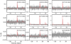 |
Fig. 11 HC3N spectra binned with a velocity resolution of 0.05 km s−1. The red lines show the results of HFS fitting. |
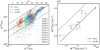 |
Fig. 12 Relations between the column densities of H2 derived from CO and dust. Upper: correlation between the column densities of H2 derived from13CO (N13CO(H2)) and C18O (NC18O(H2)) at the positions of the FAST beams for 11 PGCCs (G174.08-13.2 is not included because of lacking CO mapping observations). Data of different sources are shown in different colors. Lower: correlation between the H2 column densities at the map centers derived from dust emissions (Ndust(H2)) and C18O (NC18O(H2)). |
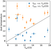 |
Fig. 13 Comparison between CO J = 1–0 excitation temperatures and Planck dust temperatures. The black line represents y = x. |
6.2 Morphologies and environments of HINSA
In the scales of source sizes, the morphologies of HINSA emission are similar to those of 13CO for most PGCCs detected with HINSA features (Figs. 9 and 10). For G165.6-09A1 and G174.4-15A1, the 13CO J = 1–0 emission and the HINSA features are weak at the map centers. This is not caused by pointing bias. In panel a and panel c of Fig. 9, the blue contours represent the emission of C2H N = 1–0 (Liu et al. 2019). At the map center of G165.6-09A1, emissions of C2H N = 1−0 were detected. Figure 14 shows the HCO+ J = 1−0 and C18O J = 2−1 emission toward the map center of G174.4-15A1. The HCO+ J = 1−0 and C18O J = 2−1 emission tends to be enhanced in the southwest corner (Fig. 14), in constract with the CO J = 1−0 emission extending to the north (panel f of Fig. 9). These results show that HINSA features are more tightly correlated with the emission of CO than that of dense gas tracers.
However, there are also several exceptions to the similarity between the emission regions of CO and HINSA. For example, in G159.2-20A1 (see the first panel of Fig. 10), this correlation is weak. For a molecular cloud, its large-scale environment and the star formation activities within it may have an influence on the existence and distribution of HINSA.
HINSA features are not detected (τ0 ≲ 0.01) at the central beam toward G165.6-09A1 and G160.51-17.07, and marginally detected (τ0 ~ 0.3) toward G159.2-20A1. There are no central-beam HINSAs detected in G165.6-09A1 and G159.2-20A1, while G160.51-17.07 has no detected HINSA anywhere. The three sources (G165.6-09A1, G160.51-17.07, and G159.2-20A1) all have Tdust larger than 19 K, the largest compared with other PGCCs (Table 1). All PGCCs are located at the margin of large-scale dust emission regions traced by the Planck 353 GHz continuum (Fig. 1). G160.51-17.07, the only PGCC showing no HINSA feature, is located within an Hα emission region represented by red contours in Fig. 1. These results all demonstrate the importance of the environments for the detection of HINSA in PGCCs and the local deviation between HINSA and CO emission regions.
Star formation activities also have significant influence on the detections of HINSA. Among 12 PGCCs, 11 have detections of HINSA, and the detection rate is 90%. HINSA features are also detected in the starless cores, L1521B. In four star formation regions, L1489E, IRAS 05413-0104, CB34, and HH25 MMs, HINSA features are only detected in CB34 and HH25 MMS. The HINSA features detected in HH25 MMS are not very reliable. HH25 MMS was observed in the tracking mode instead of the snapshot mode. There are only several (<5) beams have H I spectra with HINSA features. In the H I spectrum of HH25 MMS (Fig. 7), besides the dip with velocity similar to those of CO lines (~10 km s−1), there is another dip with redder velocity (~13 km s−1) where no corresponding CO emission lines can be seen. These two dips may be misleadingly produced by a H I emission peak between them. HINSA features tend to be inhibited by star formation activities.
Inhibitions of star formation activities on HINSA features can also be seen in PGCCs. Based on the WISE data, Marton et al. (2016) presented an all-sky catalog of 133 980 Class I/II and 608 606 Class III young stellar object (YSO) candidates. All sources in our sample have WISE YSO associations within the fields of view, except for G172.8-14A1 (see Figs. 9 and 10). The YSOs tend to locate at the margin of the HINSA detection regions, especially for sources G174.4-15A1, G175.34-10.8, G192.2-11A2, and G170.88-10.92. In G165.6-09A1, the map center is associated with four YSOs, and no HINSA feature is detected. However, at the northwest margin of G165.6-09A1, there are strong HINSA features (τHINSA ~ 0.1) but no YSO association. Since we do not know the velocities of YSOs, the YSOs matched based on angular separations may not be truly associated with PGCCs in 3D space. The relations between the distribution of YSOs and HINSA confirm that WISE YSOs are spatially related to the PGCCs, as pointed out by Marton et al. (2016) according to the YSO surface distributions around PGCCs.
Overall, HINSA tends not to be detected in regions associated with warm dust emission and background Hα emission. In the region associated with young stellar objects or dense gas emission, the HINSA feature also tends to be inhibited. Besides these effects, the varied abundances of H I in molecular clouds (Sect. 6.3) and the different excitation conditions between HINSA and CO (Sect. 6.4) may also lead to the different distributions between the HINSA and CO emission in some sources.
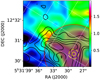 |
Fig. 14 Cutout region of G192.2-11A2 represented by the black box in Fig. 9f. The background and black contours present the emissions of C18O J = 2–1 and HCO+ J = 1–0 measured with the IRAM 30 m telescope (Xu et al., in prep.), respectively. The contours have levels from 0.5 to 0.9 stepped by 0.1 in unit of K km s−1. The red circle shows the location of the central beam of the H I observation. The yellow dashed circle and solid circle represent the beam size of HCO+ J = 1–0 and C18O J = 2–1, respectively. The white dashed lines are the grid lines of the Galactic coordinate. |
6.3 H I abundances and evolution status
The H I traced by HINSA is assumed to be well mixed with molecular gas (this issue is further discussed in Sect. 6.4). Figure 15 shows the correlation between the column densities of H I (N(H I)) derived from HINSA and the column densities of H2 (N(H2)) derived from CO spectra. N(H I) and N(H2) are positively correlated, especially for data at the map centers. The derived abundances of H I are approximately 3 × 10⁻⁴, varied by a factor of ~3. This confirms the similarity between CO and HINSA.
If a molecular cloud has a typical distance d = 400 pc, angular diameter Θ = 5′, and H I column density N(H I) = 2 × 1018 cm−2 (Table 3), the typical volume density of H I can be estimated as
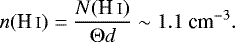 (34)
(34)
This value is consistent with the value at the steady state (nst (H I)) given by Li & Goldsmith (2003). If the beam dilution effect and the relatively large uncertainty of N(H I) (Fig. 15) are considered, the volume density of H I may exceed the nst (H I). In some work such as Tang et al. (2020) some sources with large H I abundances (~10−2) were reported, and those sources were thought to be in transition phase between atomic and molecular states.
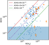 |
Fig. 15 Correlation between the column densities of H I and those of H2 derived fromC18O J = 1–0 emission. The orange squares represent the data of the central beams. The blue dots represent the data of other beams. The red square shows the data at the peak position of the HINSA map of G165.6-09A1. |
6.3.1 Production efficiency of H2 from H I
The steady-state value of H I abundance reflects the balance between the destruction rate of H2 by cosmic rays and the formation rate of H2 on the grain surfaces. However, the formation efficiency of H2 relies on the temperature and grain types. When the dust temperature is low (typically several K depending on the binding energies of hydrogen), the grain will be covered by a monolayer of H I or H2, which prevents H I further sticking onto the grain surface (Hollenbach & Salpeter 1971). When the dust temperature is higher (> 15 K in astrophysical environments; Katz et al. 1999), the formation efficiency of H2 is small since the depleted H I will be thermally desorbed before reacting with another H I. Thus, H2 will only be efficiently produced within a narrow temperature range (Hollenbach & Salpeter 1971; Katz et al. 1999). The H2 formation at higher temperature can be efficient if chemisorption site is taken into consideration (Cazaux & Tielens 2002), and this has a much higher binding energy (~104 K) than the value for the physisorption site (~500 K) and provides a shield for H I when the dust temperature is high (>20 K).
The assumption that a physisorption site occupied by one H I will not further absorb another H I is not necessary. When the dust temperature is low, there may be several H I in a single physisorption site. The bound energy of H-H is 4.52 eV (Duley 1996). If the reaction heat of a forming H2 is able to peel all H atoms in that site from grain surface, only the empty site is then truly capable of absorbing H I in gas phase. Under this assumption, the formation efficiency of H2 is not altered, and absorption and synthesis of other elements and molecules on grain surface at low dust temperatures will not be weakened by the occupation of sites by hydrogens. The production efficiency of H2 depends on the grain properties.
6.3.2 Evolution status
The sources with a relatively higher abundance of H I may still be in steady state if their dust temperatures and grain properties are not suitable for H2 formation. There is no HINSA in G160.51-17.07, which has a relatively high dust temperature (19.2 K) but not a weak CO emission (Fig. 4). However, we cannot rule out that G160.51-17.07 is in transition phase, considering its relatively lower surface density of dust compared with other PGCCs (Table 1).
The derived value of n(H I) for PGCCs may also be underestimated. It is not sure if the column densities of H I are evenly distributed within regions shown HINSA features. The beam dilution effect may be not ignorable, just like the case of CO emission.
6.4 Does the HINSA we detected trace molecular gas?
We assumed that HINSA mainly traces H I that is well mixed with molecular gas in Sect. 6.3, based on the fact that the morphologies of HINSA emissions are overall correlated to those of 13CO in PGCCs (Sect. 6.2). However, it is still not clear if the H I absorption contributed by the H I component around molecular gas cloud is also important. The spatial resolution of the H I observations of this present work prevents us from digging deeply into this issue. However, from the discussion below about the excitation status of HINSA against background H I emission, we try to illustrate that H I traced by HINSA should be a gas component of molecular cloud and confined within and around CO emission regions.
6.4.1 Collisional excitation of HINSA
The H-H spin-exchange collision is the main mechanism of the collisional excitation of H I if the abundance of H atom overwhelm that of electron (Field 1958; Furlanetto & Furlanetto 2007). The coefficient of H-H spin-exchange collision tabulated in Col. (4) of Table 2 of  of Zygelman (2005) can be empirically fit as
 (35)
(35)
for 10 < Tk < 300 K.
In optically thin conditions, the excitation temperature of HINSA can be estimated through (Purcell & Field 1956; Li & Goldsmith 2003)
 (36)
(36)
in which
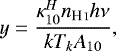 (37)
(37)
Tk is the kinematic temperature, Tbackground is the brightness temperature of background emission, nH I is the volume density of hydrogen atom (the major collision partner to excitate the H I 21 cm line), and A1,0 is the spontaneous decay rate 2.85 × 10⁻¹⁵ s−1 (Wild 1952).
If Tk = 10 K is adopted, Eqs. (35) and (37) lead to y ~ 6.9nH I. Here, nH I is in units of cm−3. For cold H I within a molecular cloud, if we further adopt nH I as the typical volume density of H I given by Eq. (34) or the steady-state value, the value of y would be larger than seven. If HINSA is not fully excited, the density of H I given by Eq. (34) will be underestimated, which leads to an even larger value of y. Thus, within a molecular cloud, the density of H I in steady state should be larger than the critical density of HINSA. If a molecular cloud is in transition phase or has grain properties not suitable for H2 formation (Sect. 6.3), its density of H I would be even higher. It is safe to assume that cold H I within molecular cloud is collisionally excited.
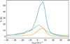 |
Fig. 16 Blue line: average H I spectrum of the observed sources in this work. Orange line:
|


6.4.2 External excitation of HI 21 cm line
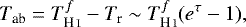
For a diffuse gas component around a molecular cloud with high abundance but low H atom density, the H I 21 cm line may be mainly excited by the background emission. The L-band continuum brightness temperature (TLband) is on average smaller than4 K (Sect. 4). This is consistent with the value estimated adopting the intensity of L-band standard interstellar radiation field (ISRF) as ~0.8 K (Winnberg et al. 1980; Li & Goldsmith 2003) and that of the cosmic microwave background as 2.73 K. If TL band is adopted as the intensity of external emission, the absorption feature contributed by diffuse H I component may not be ignorable.
We note that the L-band external emission is mainly contributed by  , the brightness temperature of the averaged background H I emission:
 (38)
(38)
The sources we observed all have |VLSR|≲ 10 km s−1 and Galactic latitude |b|≲ 20°. The mean value of |b| is 14°. The lower limit of the intensity of  can be estimated through multiplying the average spectrum of observed sources by sin (14°), as shown in Fig. 16. The peak intensity of
  is expected to be ~14 K. This is confirmed by the H I spectrum averaged over the all-sky spectra from the HI4PI survey (HI4PI Collaboration 2016), which gives brightness temperatures of ~20, ~10, and ~5 K for VLSR = 0, 10, and 20 km s−1, respectively (Fig. 16). These values are larger than TL band.
For a molecular cloud with short distance to the Earth and thus similar  compared with that seen from the Earth, Tbackground will be dominated by the average brightness temperature of H I 21 cm spectra if |VLSR| is small (|VLSR| < 20 km s−1). If
  is small, the warmer and diffuser H I around the molecular cloud may be excited by TL band. Then, the H I in the diffuse gas may also contribute absorption features similar to HINSA and make us overestimate the column density of cold H I associated with molecular gas. If
  is not ignorable, the diffuse H I will not contribute much absorption, even if it is not collisionally excited. Then, we can safely assume that the HINSA features we extracted are tightly associated with molecular gas. This effect inhibits the possible absorption contributed by the outer diffuse H I-rich shell of a molecular cloud, and it confines HINSA within molecular cloud.
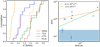 |
Fig. 17 Comparisons between the velocity dispersions and column densities of HC3N and H I. Left: cumulative distributions of velocity dispersions. Solid lines and dashed lines represent σ and σNT, respectively (Sect. 6.5). Right: correlation between the column densities of H I and those of HC3N. Green and orange lines represent the linear fitting with and without the two data in blue shadowing, respectively. For data in the blue shadowing, the N(H I) parameters are not reliable with regard to the fit optical depth of HINSA τ < 0.01 (Sect. 5.2.5). |
6.4.3 HINSA and CO emission region
A molecular cloud may contain both CO-bright gas and CO-dark gas (e.g. Bolatto et al. 2013). In molecular region with lower gas density, the H I abundance should be higher with the volume density of H I unchanging. There may also be HINSA features produced in CO-dark regions. However, HINSA features can be restrained because the cloud tends to be warmer in low-density regions. CO is important for the cooling of molecular clouds (Goldsmith & Langer 1978). For a molecular cloud with n(H2) = 103 cm−3, Tk = 10 K, and abundance of CO XCO = 2 × 10⁻⁴, the cooling rate contributed by CO emission is (Whitworth & Jaffa 2018)
 (39)
(39)
The heatingrate contributed by cosmic rays and X-rays is (Glassgold & Langer 1973)
 (40)
(40)
If n(H2) is smaller than 103 cm−3, CO cooling is not effective enough, and the gas will be warmer and unfavorable to HINSA. The density threshold 103 cm−3 is also the lower limit for the excitations of CO transitions, and this is another reason why HINSA features are confined around CO emission regions. PGCCs may be the coldest and earliest samples showing HINSA features. Overall, the non-small  and CO cooling both help to confine HINSA features to regions within and around CO emission kernels.
6.5 HINSA and HC3N
The velocity dispersions (σ) can be derived from the line widths (ΔV) through
 (41)
(41)
The nonthermal velocity dispersions (σNT) can be calculated through
 (42)
(42)
where mX represents the mass of molecule X. The left panel of Fig. 17 shows the cumulative distributions of σ and σNT for HINSA, 13CO, C18O and HC3N. σHC_3N is similar to σ13CO, and tends to be larger than σC18O. However, the nonthermal velocity dispersion traced by HINSA is comparable with that of C18O. The broadening effect introduced by the possible thick optical depth of 13CO J = 1–0 cannot fully explain the larger σNT traced by 13CO compared with those traced by C18O. An optical depth of 2 contributes to line widths smaller than 30% (Phillips et al. 1979). 13CO may trace more extended gas component compared with C18O because 13CO J = 1–0 has larger optical depth compared with C18O J = 1–0 and is easier to be excited. HINSA and C18O J = 1–0 are optically thin in molecular clouds, and originate from similar regions. However, the spectra of HC3N are quite narrow, with line widths (<0.1 km s−1 ; Fig. 17) smaller than those of HINSA and 13CO.
Previous observations show that HC3N is abundant in some but not all starless cores (Suzuki et al. 1992; Wu et al. 2019b). In low-mass, star formation regions, HC3N will be enhanced again under the heating of YSOs in early stages (Sakai et al. 2008, 2009), but it may be destroyed by radiation from YSOs (Liu et al. 2021). In molecular cloud harboring young stars, it is also correlated with outflows and shocks (Wu et al. 2019b; Yu et al. 2019). The narrow line widths of HC3N J = 2–1 imply that the HC3N emission may originate from more compact gas component within PGCCs, instead of the outer regions dissociated by external radiation fields or shocked by turbulent flows. Although its CO emission is extended (Sect. 6.1), the PGCC could harbor dense and compact regions. The narrow line widths of HC3N confirm that these PGCCs are in a quiescent state. Carbon chain molecule abundant PGCCs have both cold and condensed structures at the center regions traced by HC3N and extended gas components at the outer regions traced by CO. This makes them good targets to observe and study HINSA.
The right panel of Fig. 17 shows the correlation between the column density of H I derived from HINSA and the column densities of HC3N. There is a weak positive correlation between N(HC3N) and N(H I), and the abundance ratio N(HC3N)/N(H I) is ~10−5. The PGCCs with the strongest HC3N emission tend to have more remarkable HINSA features. However, there is not enough evidence to assert that HINSA in sources with weak HC3N emission will be suppressed. The G178.98-06.7 is one such source with no detection of HC3N but with strong HINSA. This is not a surprise since not all PGCCs are CCM abundant, and the detection rate of HINSA is considerablein PGCCs with no previous observations of CCM emission (Tang et al. 2020). The prior of the presence of HC3N raises the detection rate of HINSA close to ~90% in PGCCs of this work, although the sample size is still limited.
7 Summary
Twelve PGCCs, one starless core L1521B, and four star forming sources were searched for H I narrow-line self-absorption (HINSA) features using the FAST. Combining the data of H I 21 cm lines, CO J = 1–0, HC3N J = 2–1, and dust continuum, we studied the morphologies, abundances, and excitation conditions of HINSA, CO, and HC3N in PGCCs and star forming sources. We also investigated the relations between these parameters and the environments.
The main results are as follows:
- 1.
HINSA features are detected in 11 of 12 PGCCs, corresponding to a detection rate of 90%. Eight of the detected ones have HC3N emissions.
- 2.
We improved the method of extracting HINSA features (method 2) based on the method of Krčo et al. (2008) (method 1). The S/N thresholds of the two methods are deduced. Method 2 has a much lower S/N requirement compared to method 1. Method 2 performs better when extracting HINSA features with low S/Ns, and large line widths resulting from blended components or high velocity resolution.
- 3.
The line widths and velocities of CO lines are adopted as the initial values of the fitting parameters of HINSA. Applying the improved method, HINSA features are extracted in 11 of 12 PGCCs, the starless core L1251B, and two of four star forming sources. If method 1 was applied, HINSA features can only be extracted in L1251B and seven PGCCs.
- 4.
The optical depths and line widths of HINSA, and the column densities of H I were obtained. The abundances of cold H I in PGCCs are approximately 3 × 10⁻⁴, varied bya factor of ~3.
- 5.
HINSA tends not to be detected in regions associated with warm dust emission, background ionizing radiations, stellar objects, and dense gas emission.
- 6.
The distribution of HINSA is similar to that of CO emission. External excitation by the background H I emission and the CO cooling both helps to confine HINSA features to regions within and around CO emission kernels.
- 7.
CO emission looks as extended as the Planck dust continuum. Part of the CO emission may come from more diffuse regions besides the regions associated with the cold dust or dense gas.
- 8.
HFS fittings are applied to HC3N J = 2–1. The column densities of HC3N are calculated. The average abundance of HC3N is 2.2(±0.8) × 10−9. The nonthermal dispersions traced by HINSA are comparable with those of C18O, and larger than those of HC3N. HC3N emissions may originate from the condensed regions within PGCCs. CCM-abundant PGCCs provide a good sample to study HINSA.
Guided by CCM emissions, HINSA can be a good tool to detect and analyze the extended neutral gas components in PGCCs. The sample size of this work is limited. It would be helpful to search more PGCCs in the future, with the supports of the good sensitivity of the FAST and the improved HINSA extracting method.
Acknowledgements
This project was supported by the National Key R&D Program of China No. 2017YFA0402600, and the NSFC No. 12033005, 11433008, 11725313, 11373009, 11503035 and 11573036. N.-Y.T. is supported by National Key R&D Program of China No. 2018YFE0202900 and NSFC No. 11803051. K.W. acknowledges support by the National Science Foundation of China (12041305, 11973013), and the High-performance Computing Platform of Peking University through the instrumental analysis fund of Peking University (0000057511). We are grateful to the help of the staff of the FAST during the observations and data conduction. We show warm thanks to the anonymous referee for providing many constructive argues and suggestions which make the content of this work more substantial and clear.
References
- Baker, P. L., & Burton, W. B. 1979, A&AS, 35, 129 [NASA ADS] [Google Scholar]
- Bolatto, A. D., Wolfire, M., & Leroy, A. K. 2013, ARA&A, 51, 207 [CrossRef] [Google Scholar]
- Bussa, S., & VEGAS Development Team 2012, AAS Meeting Abs., 219, 446.10 [NASA ADS] [Google Scholar]
- Cameron, A. G. W. 1962, Icarus, 1, 13 [NASA ADS] [CrossRef] [Google Scholar]
- Cazaux, S., & Tielens, A. G. G. M. 2002, ApJ, 575, L29 [NASA ADS] [CrossRef] [Google Scholar]
- Codella, C., & Scappini, F. 2003, MNRAS, 344, 1257 [NASA ADS] [CrossRef] [Google Scholar]
- Dickey, J. M., Kulkarni, S. R., van Gorkom, J. H., & Heiles, C. E. 1983, ApJS, 53, 591 [NASA ADS] [CrossRef] [Google Scholar]
- Duley, W. W. 1996, MNRAS, 279, 591 [NASA ADS] [CrossRef] [Google Scholar]
- Ewen, H. I., & Purcell, E. M. 1951, Nature, 168, 356 [NASA ADS] [CrossRef] [Google Scholar]
- Field, G. B. 1958, Proc. IRE, 46, 240 [NASA ADS] [CrossRef] [Google Scholar]
- Finkbeiner, D. P. 2003, ApJS, 146, 407 [Google Scholar]
- Frerking, M. A., Langer, W. D., & Wilson, R. W. 1982, ApJ, 262, 590 [Google Scholar]
- Furlanetto, S. R., & Furlanetto, M. R. 2007, MNRAS, 379, 130 [CrossRef] [Google Scholar]
- Garden, R. P., Hayashi, M., Hasegawa, T., Gatley, I., & Kaifu, N. 1991, ApJ, 374, 540 [NASA ADS] [CrossRef] [Google Scholar]
- Gibb, A. G., & Davis, C. J. 1997, IAU Symp. 182, 120 [Google Scholar]
- Gibb, A. G., & Davis, C. J. 1998, MNRAS, 298, 644 [NASA ADS] [CrossRef] [Google Scholar]
- Gibson, S. J. 2010, ASP Conf. Ser., 438, 111 [Google Scholar]
- Gibson, S. J., Taylor, A. R., Higgs, L. A., & Dewdney, P. E. 2000, ApJ, 540, 851 [NASA ADS] [CrossRef] [Google Scholar]
- Glassgold, A. E., & Langer, W. D. 1973, ApJ, 186, 859 [NASA ADS] [CrossRef] [Google Scholar]
- Goldsmith, P. F., & Langer, W. D. 1978, ApJ, 222, 881 [Google Scholar]
- Goldsmith, P. F., & Li, D. 2005, ApJ, 622, 938 [NASA ADS] [CrossRef] [Google Scholar]
- Gould, R. J., & Salpeter, E. E. 1963, ApJ, 138, 393 [NASA ADS] [CrossRef] [Google Scholar]
- Heiles, C. 2001, ApJ, 551, L105 [CrossRef] [Google Scholar]
- Heiles, C., Li, D., McClure-Griffiths, N., Qian, Le., & Liu, S. 2019, Res. Astron. Astrophys., 19, 017 [CrossRef] [Google Scholar]
- HI4PI Collaboration (Ben Bekhti, N., et al.) 2016, A&A, 594, A116 [NASA ADS] [CrossRef] [EDP Sciences] [Google Scholar]
- Hirota, T., Maezawa, H., & Yamamoto, S. 2004, ApJ, 617, 399 [Google Scholar]
- Hollenbach, D., & Salpeter, E. E. 1971, ApJ, 163, 155 [NASA ADS] [CrossRef] [Google Scholar]
- Jiang, P., Yue,Y., Gan, H., et al. 2019, Sci. China Phys. Mech. Astron., 62, 959502 [NASA ADS] [CrossRef] [Google Scholar]
- Juvela, M., Ristorcelli, I., Marshall, D. J., et al. 2015, A&A, 584, A93 [NASA ADS] [CrossRef] [EDP Sciences] [Google Scholar]
- Katz, N., Furman, I., Biham, O., Pirronello, V., & Vidali, G. 1999, ApJ, 522, 305 [NASA ADS] [CrossRef] [Google Scholar]
- Kavars, D. W., Dickey, J. M., McClure-Griffiths, N. M., Gaensler, B. M., & Green, A. J. 2005, ApJ, 626, 887 [NASA ADS] [CrossRef] [Google Scholar]
- Khanzadyan, T., Smith, M. D., Gredel, R., Stanke, T., & Davis, C. J. 2002, A&A, 383, 502 [NASA ADS] [CrossRef] [EDP Sciences] [Google Scholar]
- Knapp, G. R. 1974, AJ, 79, 527 [NASA ADS] [CrossRef] [Google Scholar]
- Krčo, M., & Goldsmith, P. F. 2010, ApJ 724, 1402 [CrossRef] [Google Scholar]
- Krčo, M., Goldsmith, P. F., Brown, R. L., & Li, D. 2008, ApJ, 689, 276 [CrossRef] [Google Scholar]
- Kwok, S. 2007, Physics and Chemistry of the Interstellar Medium (Cambridge: Cambridge University Press) [Google Scholar]
- Lee, C. W., & Myers, P. C. 1999, ApJS, 123, 233 [NASA ADS] [CrossRef] [Google Scholar]
- Li, D., & Goldsmith, P. F. 2003, ApJ, 585, 823 [NASA ADS] [CrossRef] [Google Scholar]
- Li, J., Shen, Z.-Q., Wang, J., et al. 2016, ApJ, 824, 136 [Google Scholar]
- Li, D., Wang, P., Qian, L., et al. 2018, IEEE Microw. Mag., 19, 112 [CrossRef] [Google Scholar]
- Liu, T., Wu, Y., & Zhang, H. 2012, ApJS, 202, 4 [NASA ADS] [CrossRef] [Google Scholar]
- Liu, T., Wu, Y., & Zhang, H. 2013, ApJ, 775, L2 [NASA ADS] [CrossRef] [Google Scholar]
- Liu, X. C., Wu, Y., Zhang, C., et al. 2019, A&A, 622, A32 [EDP Sciences] [Google Scholar]
- Liu, X.-C., Wu, Y., Zhang, C., et al. 2021, ApJ, 912, 148 [NASA ADS] [CrossRef] [Google Scholar]
- Lockman, F. J. 1984, ApJ, 283, 90 [NASA ADS] [CrossRef] [Google Scholar]
- Mangum, J. G., & Shirley, Y. L. 2015, PASP, 127, 266 [Google Scholar]
- Marton, G., Tóth, L. V., Paladini, R., et al. 2016, MNRAS, 458, 3479 [Google Scholar]
- McCutcheon, W. H., Shuter, W. L. H., Dickman, R. L., & Roger, R. S. 1980, ApJ, 237, 9 [NASA ADS] [CrossRef] [Google Scholar]
- Meng, F., Wu, Y., & Liu, T. 2013, ApJS, 209, 37 [NASA ADS] [CrossRef] [Google Scholar]
- Myers, P. C., Heyer, M., Snell, R. L., & Goldsmith, P. F. 1988, ApJ, 324, 907 [Google Scholar]
- Nakanishi, H., & Sofue, Y. 2003, PASJ, 55, 191 [Google Scholar]
- Nan, R., Li, D., Jin, C., et al. 2011, Int. J. Mod. Phys. D, 20, 989 [Google Scholar]
- Phillips, T. G., Huggins, P. J., Wannier, P. G., & Scoville, N. Z. 1979, ApJ, 231, 720 [Google Scholar]
- Pineda, J. L., Langer, W. D., Velusamy, T., & Goldsmith, P. F. 2013, A&A, 554, A103 [CrossRef] [EDP Sciences] [Google Scholar]
- Planck Collaboration I. 2011, A&A, 536, A1 [NASA ADS] [CrossRef] [EDP Sciences] [Google Scholar]
- Planck Collaboration XXIII. 2011, A&A, 536, A23 [NASA ADS] [CrossRef] [EDP Sciences] [Google Scholar]
- Planck Collaboration I. 2016, A&A, 594, A1 [NASA ADS] [CrossRef] [EDP Sciences] [Google Scholar]
- Planck Collaboration XVIII. 2016, A&A, 594, A28 [NASA ADS] [CrossRef] [EDP Sciences] [Google Scholar]
- Planck Collaboration XLVIII. 2016, A&A, 596, A109 [NASA ADS] [CrossRef] [EDP Sciences] [Google Scholar]
- Purcell, E. M., & Field, G. B. 1956, ApJ, 124, 542 [NASA ADS] [CrossRef] [Google Scholar]
- Reich, W. 1982, A&AS, 48, 219 [NASA ADS] [Google Scholar]
- Reich, P., & Reich, W. 1986, A&AS, 63, 205 [NASA ADS] [Google Scholar]
- Reid, M. J., Dame, T. M., Menten, K. M., & Brunthaler, A. 2016, ApJ, 823, 77 [Google Scholar]
- Reipurth, B., Davis, C. J., Bally, J., et al. 2019, AJ, 158, 107 [NASA ADS] [CrossRef] [Google Scholar]
- Remazeilles, M., Delabrouille, J., & Cardoso, J.-F. 2011, MNRAS, 418, 467 [Google Scholar]
- Sakai, N., Sakai, T., Hirota, T., & Yamamoto, S. 2008, ApJ, 672, 371 [Google Scholar]
- Sakai, N., Sakai, T., Hirota, T., Burton, M., & Yamamoto, S. 2009, ApJ, 697, 769 [Google Scholar]
- Schultheis, M., Chen, B. Q., Jiang, B. W., et al. 2014, A&A, 566, A120 [NASA ADS] [CrossRef] [EDP Sciences] [Google Scholar]
- Shetty, R., Glover, S. C., Dullemond, C. P., & Klessen, R. S. 2011, MNRAS, 412, 1686 [NASA ADS] [CrossRef] [Google Scholar]
- Shimajiri, Y., Kitamura, Y., Saito, M., et al. 2014, A&A, 564, A68 [NASA ADS] [CrossRef] [EDP Sciences] [Google Scholar]
- Suzuki, H., Yamamoto, S., Ohishi, M., et al. 1992, ApJ, 392, 551 [Google Scholar]
- Tang, N., Li, D., Heiles, C., et al. 2016, A&A, 593, A42 [NASA ADS] [CrossRef] [EDP Sciences] [Google Scholar]
- Tang, N.-Y., Zuo, P., Li, D., et al. 2020, Res. Astron. Astrophys., 20, 077 [CrossRef] [Google Scholar]
- Tang, N., Li, D., Yue, N., et al. 2021, ApJS, 252, 1 [Google Scholar]
- Taniguchi, K., Ozeki, H., Saito, M., et al. 2016, ApJ, 817, 147 [Google Scholar]
- Tauber, J. A., Norgaard-Nielsen, H. U., Ade, P. A. R., et al. 2010, A&A, 520, A2 [NASA ADS] [CrossRef] [EDP Sciences] [Google Scholar]
- Turner, B. E. 1971, ApJ, 163, L35 [NASA ADS] [CrossRef] [Google Scholar]
- Wang, J. Q., Yu, L. F., Zhao, R. B., et al. 2015, Acta Astron. Sinica, 56, 63 [Google Scholar]
- Wang, Y., Bihr, S., Beuther, H., et al. 2020, A&A, 634, A139 [NASA ADS] [CrossRef] [EDP Sciences] [Google Scholar]
- Whitworth, A. P., & Jaffa, S. E. 2018, A&A, 611, A20 [NASA ADS] [CrossRef] [EDP Sciences] [Google Scholar]
- Wild, J. P. 1952, ApJ, 115, 206 [NASA ADS] [CrossRef] [Google Scholar]
- Wilson, T. L.,& Minn, Y. K. 1977, A&A, 54, 933 [NASA ADS] [Google Scholar]
- Winkel, B., Kerp, J., Flöer, L., et al. 2016, A&A, 585, A41 [NASA ADS] [CrossRef] [EDP Sciences] [Google Scholar]
- Winnberg, A., Grasshoff, M., Goss, W. M., & Sancisi, R. 1980, A&A, 90, 176 [NASA ADS] [Google Scholar]
- Wu, Y., Wei, Y., Zhao, M., et al. 2004, A&A, 426, 503 [NASA ADS] [CrossRef] [EDP Sciences] [Google Scholar]
- Wu, Y., Liu, T., Meng, F., et al. 2012, ApJ, 756, 76 [CrossRef] [Google Scholar]
- Wu, Y., Lin, L., Liu, X., et al. 2019a, A&A, 627, A162 [NASA ADS] [CrossRef] [EDP Sciences] [Google Scholar]
- Wu, Y., Liu, X., Chen, X., et al. 2019b, MNRAS, 488, 495 [Google Scholar]
- Xie, J., Fuller, G. A., Li, D., et al. 2021, Sci. China Phys. Mech. Astron., 64, 279511 [NASA ADS] [CrossRef] [Google Scholar]
- Xu, F., Wu, Y., Liu, T., et al. 2021, ApJ, 920, 103 [NASA ADS] [CrossRef] [Google Scholar]
- Yen, H.-W., Takakuwa, S., Ohashi, N., et al. 2014, ApJ, 793, 1 [NASA ADS] [CrossRef] [Google Scholar]
- Yu, N., Wang, J.-J., & Xu, J.-L. 2019, MNRAS, 489, 4497 [CrossRef] [Google Scholar]
- Yun, J. L., & Clemens, D. P. 1994, ApJS, 92, 145 [NASA ADS] [CrossRef] [Google Scholar]
- Zhang, T., Wu, Y., Liu, T., & Meng, F. 2016, ApJS, 224, 43 [NASA ADS] [CrossRef] [Google Scholar]
- Zhang, K., Wu, J., Li, D., et al. 2019, Sci. China Phys. Mech. Astron., 62, 959506 [Google Scholar]
- Zhang, C., Wu, Y., Liu, X., et al. 2020, ApJS, 247, 29 [NASA ADS] [CrossRef] [Google Scholar]
- Zhang, C., Wu, Y., Liu, X. C., et al. 2021, A&A, 648, A83 [NASA ADS] [CrossRef] [EDP Sciences] [Google Scholar]
- Zuo, P., Li, D., Peek, J. E. G., et al. 2018, ApJ, 867, 13 [NASA ADS] [CrossRef] [Google Scholar]
- Zygelman, B. 2005, ApJ, 622, 1356 [NASA ADS] [CrossRef] [Google Scholar]
All Tables
All Figures
|
Fig. 1 Galactic longitude-latitude positions of the 17 sources in our sample. Yellow and cyan hexagons represent the 12 PGCCs and the other five sources, respectively. The size of the hexagon represents the covering area of the 19-beam receiver of the FAST. The dot within each hexagon shows targeted locations of the central beam (Beam 1; Fig. 2). The background image shows Planck dust temperature distribution. The black contours with levels of 3, 7, and 11 Myr sr−1 represent the Planck 850 μm continuum. The red contours represent the Hα emission (Finkbeiner 2003) in units of R (106∕4π photons cm−2 s−1 sr−1), with levels from 15 to 215 stepped by 40. |
| In the text | |
|
Fig. 2 Configuration of the 19-beam receiver of FAST (Li et al. 2018). Each snapshot mode observation consists of four single-point-mode observations. Equatorial coordinate system is adopted for the tracking mode, while Galactic coordinate system is adopted for the snapshot mode. |
| In the text | |
|
Fig. 3 Blue and orange solid line are the H I 21 cm spectra obtained by the FAST beam 1 and beam 8, respectively. The spectra werecalibrated adopting a beam efficiency of 0.85 for extended source. The red dotted lines are the spectra from the EBHIS (Winkel et al. 2016). The black solid lines are the FAST H I 21 cm spectra smoothed to have a velocity resolution similar to that of the EBHIS spectrum. To avoid overlapping, the red dotted lines and the black solid lines have been moved up by 10 and 20 K for beam 1 and beam 8, respectively. |
| In the text | |
|
Fig. 4 Spectra of J = 1–0 of 12CO, C13O, and C18O (Wu et al. 2012) are shown from top to bottom in each panel. |
| In the text | |
|
Fig. 5 HINSA features of G174.4-15A1 extracted by method 1 (left) and method 2 (right). Method 1 fails to fit the HINSA component because of the low S/N and the blending of two absorption components with similar velocities. In each panel, the gray line is the observed spectrum Tr, the blue line is the recovered TH I, and the red line is Tab. The Tab shown here has been multiplied by a factor of five. |
| In the text | |
 |
Fig. 6 Same as Fig. 5, but for G170.88-10.92. |
| In the text | |
|
Fig. 7 H I 21 cm spectra at the center beam. In each panel, the gray line is the observed spectrum Tr, the blue line is the recovered TH I using method 2, and the red line is Tab. Values of Tab on the y-axis range from 0 to 20 K for all sources except G174.08-13.2, which uses 0–60 K. The orange and blue squares represent the sources that can and cannot be successfully fit using method 1. The blue line is not shown for spectrum with fit τ smaller than 0.01. |
| In the text | |
|
Fig. 8 Distribution of S/Nc and S/N(Tab) for the H I spectra of the central beams (Table 3). Here, S/N(Tab) is the ratio between the intensity of absorption dip revealed by method 2 and the spectra noise, and S/Nc is the signal-to-noise threshold required by method 1 (Sect. 5.2.2). The orange and blue squares represent the sources that can and cannot be successfully fit using method 1, respectively. The black line represents x = y. As predicted, the black line is the separation line between the two cases. |
| In the text | |
|
Fig. 9 Backgrounds: strengths of HINSA measured in the snapshot mode, extracted using method 2. Black contours: 13CO J = 1–0 emissions, which have been smoothed to the angular resolution of H I observations. Big black boxes: areas covered by CO data. Blue crosses: sampled points of the FAST, and red circle: center beam. Small red boxes and triangles: Class I/II and Class III YSOs. In panels a and c, the white contours represent the emission of C2H N = 1–0 within the white rectangles (Liu et al. 2019). In panel f, the small black rectangle represents the mapped region of the IRAM HCO+ J = 1–0 and C18O J = 2–1 observations, which are shown in Fig. 14. |
| In the text | |
|
Fig. 10 Backgrounds: strengths of HINSA measured in the tracking mode. Symbols have the same meanings with those in Fig. 9. |
| In the text | |
|
Fig. 11 HC3N spectra binned with a velocity resolution of 0.05 km s−1. The red lines show the results of HFS fitting. |
| In the text | |
|
Fig. 12 Relations between the column densities of H2 derived from CO and dust. Upper: correlation between the column densities of H2 derived from13CO (N13CO(H2)) and C18O (NC18O(H2)) at the positions of the FAST beams for 11 PGCCs (G174.08-13.2 is not included because of lacking CO mapping observations). Data of different sources are shown in different colors. Lower: correlation between the H2 column densities at the map centers derived from dust emissions (Ndust(H2)) and C18O (NC18O(H2)). |
| In the text | |
|
Fig. 13 Comparison between CO J = 1–0 excitation temperatures and Planck dust temperatures. The black line represents y = x. |
| In the text | |
|
Fig. 14 Cutout region of G192.2-11A2 represented by the black box in Fig. 9f. The background and black contours present the emissions of C18O J = 2–1 and HCO+ J = 1–0 measured with the IRAM 30 m telescope (Xu et al., in prep.), respectively. The contours have levels from 0.5 to 0.9 stepped by 0.1 in unit of K km s−1. The red circle shows the location of the central beam of the H I observation. The yellow dashed circle and solid circle represent the beam size of HCO+ J = 1–0 and C18O J = 2–1, respectively. The white dashed lines are the grid lines of the Galactic coordinate. |
| In the text | |
|
Fig. 15 Correlation between the column densities of H I and those of H2 derived fromC18O J = 1–0 emission. The orange squares represent the data of the central beams. The blue dots represent the data of other beams. The red square shows the data at the peak position of the HINSA map of G165.6-09A1. |
| In the text | |
|
Fig. 16 Blue line: average H I spectrum of the observed sources in this work. Orange line:
|
| In the text | |
|
Fig. 17 Comparisons between the velocity dispersions and column densities of HC3N and H I. Left: cumulative distributions of velocity dispersions. Solid lines and dashed lines represent σ and σNT, respectively (Sect. 6.5). Right: correlation between the column densities of H I and those of HC3N. Green and orange lines represent the linear fitting with and without the two data in blue shadowing, respectively. For data in the blue shadowing, the N(H I) parameters are not reliable with regard to the fit optical depth of HINSA τ < 0.01 (Sect. 5.2.5). |
| In the text | |
Current usage metrics show cumulative count of Article Views (full-text article views including HTML views, PDF and ePub downloads, according to the available data) and Abstracts Views on Vision4Press platform.
Data correspond to usage on the plateform after 2015. The current usage metrics is available 48-96 hours after online publication and is updated daily on week days.
Initial download of the metrics may take a while.