| Issue |
A&A
Volume 654, October 2021
|
|
|---|---|---|
| Article Number | A88 | |
| Number of page(s) | 35 | |
| Section | Extragalactic astronomy | |
| DOI | https://doi.org/10.1051/0004-6361/202141558 | |
| Published online | 19 October 2021 | |
Mapping the “invisible” circumgalactic medium around a z ∼ 4.5 radio galaxy with MUSE
1
Astronomisches Rechen-Institut, Zentrum für Astronomie der Universität Heidelberg, Mönchhofstr. 12-14, 69120 Heidelberg, Germany
e-mail: wuji.wang@uni-heidelberg.de; wuji.wang_astro@outlook.com
2
European Southern Observatory, Karl-Schwarzchild-Str. 2, 85748 Garching, Germany
3
Instituto de Astrofísica e Ciências do Espaço, Universidade do Porto, CAUP, Rua das Estrelas, 4150-762 Porto, Portugal
4
Centro de Astrobiología, CSIC-INTA, Ctra. de Torrejón a Ajalvir, km 4, 28850 Torrejón de Ardoz, Madrid, Spain
5
Univ. Lyon, Univ. Lyon1, ENS de Lyon, CNRS, Centre de Recherche Astrophysique de Lyon UMR5574, 69230 Saint-Genis-Laval, France
6
Inter-University Institute for Data Intensive Astronomy, Department of Astronomy, University of Cape Town, Rondebosch 7701, South Africa
7
Physics Department, University of Johannesburg, 5 Kingsway Ave, Rossmore, Johannesburg 2092, South Africa
Received:
16
June
2021
Accepted:
19
July
2021
In this paper we present Multi Unit Spectroscopic Explorer integral field unit spectroscopic observations of the ∼70 × 30 kpc2 Lyα halo around the radio galaxy 4C04.11 at z = 4.5077. High-redshift radio galaxies are hosted by some of the most massive galaxies known at any redshift and are unique markers of concomitant powerful active galactic nucleus (AGN) activity and star formation episodes. We map the emission and kinematics of the Lyα across the halo as well as the kinematics and column densities of eight H I absorbing systems at −3500 < Δv < 0 km s−1. We find that the strong absorber at Δv ∼ 0 km s−1 has a high areal coverage (30 × 30 kpc2), being detected across a large extent of the Lyα halo, a significant column density gradient along the southwest to northeast direction, and a velocity gradient along the radio jet axis. We propose that the absorbing structure, which is also seen in C IV and N V absorption, represents an outflowing metal-enriched shell driven by a previous AGN or star formation episode within the galaxy and is now caught up by the radio jet, leading to jet-gas interactions. These observations provide evidence that feedback from AGN in some of the most massive galaxies in the early Universe may play an important role in redistributing material and metals in their environments.
Key words: galaxies: evolution / galaxies: active / galaxies: high-redshift / galaxies: individual: 4C04.11 / galaxies: halos
© ESO 2021
1. Introduction
There is significant observational and theoretical evidence that supermassive black holes (SMBHs) in the centers of galaxies play a crucial role in the evolution of their hosts (e.g., Ho 2008). The powerful nuclear activities caused by actively accreting SMBHs – active galactic nuclei (AGN) – can lead to a substantial release of energy (Silk & Rees 1998) and impact the evolution of their host galaxies (Kormendy & Ho 2013; Heckman & Best 2014). The most powerful AGN (quasars, Lbol > 1045 erg s−1) can easily heat and photo-ionize their surrounding gas, sometimes even on scales of tens of kiloparsecs, well into the circumgalactic medium (Tumlinson et al. 2017). The detailed mechanisms and timescales relevant to AGN-driven feedback are still not fully understood (Fabian 2012), but large samples of galaxies with high spatial resolution using the modern surveys, primarily at low redshift right now, for example Sloan Digital Sky Survey-IV Mapping Nearby Galaxies at Apache Point Observatory (SDSS-IV MaNGA, e.g., Wylezalek et al. 2018), help in assessing its prevalence and nature. However, it is the epoch at z ∼ 2 − 3 that marks the peak of both star formation and quasar activity (cosmic noon, z ∼ 2 − 3; Madau & Dickinson 2014; Förster Schreiber & Wuyts 2020), and probing the feedback processes in AGN at that epoch is essential.
The CGM (see Tumlinson et al. 2017, for a detailed review) is now understood to be a key component in disentangling the feedback processes in active galaxies. It links the smaller-scale interstellar medium (ISM) of the galaxy to the larger-scale intergalactic medium (IGM), not only in a geometrical way but also by acting as the reservoir fueling star formation and the central black hole, where the feedback interacts with the galactic environment and where the gas recycling during galaxy evolution is controlled. This complex environment is multiphase and has been observed in numerous surveys (e.g., Tumlinson et al. 2013; Bordoloi et al. 2014; Peek et al. 2015; Borthakur et al. 2015) at low redshift. A prominent feature of the CGM around active galaxies is the Lyα (Lyman-α) emission line, which is also ubiquitously observed at high redshift (e.g., Haiman & Rees 2001; Reuland et al. 2003; van Breugel et al. 2006; Villar-Martín 2007; Humphrey et al. 2013; Cantalupo et al. 2014; Wisotzki et al. 2016, 2018; Arrigoni Battaia et al. 2018, 2019; Nielsen et al. 2020). Lyα is the transition of the hydrogen electron from the 2p orbit to its ground state. It can happen primarily through collisional excitation and recombination (see Dijkstra 2014, 2017, for a detailed review of Lyα emission mechanisms and radiative transfer). In extragalactic studies, the recombination production of Lyα emission can be generated by photoionization by young stars and/or AGN (fluorescence). This fluorescence emission on larger scales (CGM and IGM) can also be due to UV background radiation. Additionally, collisional excitation can play an important role in the emission seen in outflows and infalling gas (Ouchi et al. 2020). The bright Lyα emission line, along with other UV lines excited by the central or background sources, provides a useful tool for studying the galactic environments in the early Universe. Additionally, H I and metal absorption features observed in the CGM are powerful tracers of feedback signatures as well as tracers of infalling pristine gas (e.g., low metallicity absorption in a z ∼ 2.7 submillimeter galaxy; Fu et al. 2021). The sensitive integral field spectrographs on the largest ground-based telescopes, such as MUSE (Multi-Unit Spectroscopic Explorer; Bacon et al. 2010, 2014) and KCWI (Keck Cosmic Web Imager; Morrissey et al. 2012; see Cai et al. 2019 for observation of Lyα halos with KCWI), are perfectly suited for mapping these UV features as they move into the optical band for high-redshift sources.
This paper focuses on the population of high-redshift radio galaxies (HzRGs; L500 MHz > 1026 W Hz−1Miley & De Breuck 2008), which are some of the most massive galaxies known at any redshift (with a narrow range in stellar masses of (1 − 6)×1011 M⊙ for 1 < z < 5.2; De Breuck et al. 2010). Their energetic radio jets are unique markers of concomitant powerful AGN activity, which place them amongst the most active sources at and near cosmic noon. High-redshift radio galaxies have furthermore been shown to be powerful beacons of dense (proto-)cluster environments in the early Universe (e.g., Le Fevre et al. 1996; Stern et al. 2003; Venemans et al. 2002, 2003, 2004, 2005, 2007; Wylezalek et al. 2013). The quasar-level AGN activity (Miley & De Breuck 2008) at the center is blocked by the thick dusty torus acting as the “coronograph” (Vernet et al. 2001); this makes HzRGs true obscured type-2 quasars, allowing us to probe their host galaxies and CGM without strong AGN contamination (e.g., for unobscured quasars, see Arrigoni Battaia et al. 2019, and for radio-quite type-2 sources, see Cai et al. 2017). Comprehensive studies using near-infrared integral field unit (IFU) instruments show that the ionized gas in HzRGs is highly perturbed (FWHM ∼ 1000 km s−1) at kiloparsec scales and is aligned with the radio jets (Nesvadba et al. 2006, 2007, 2008, 2017a,b; Collet et al. 2015, 2016). This implies that the energy and momentum transfer between the central quasar and their ISM is likely due to the jets. Radio-mode feedback may therefore play a fundamental role during the evolution of HzRGs. Recently, Falkendal et al. (2019) combined infrared and millimeter data and deduced a more robust result of a relatively low star formation rate (SFR) for a sample of HzRGs, suggesting evidence of rapid quenching compared to previous studies (e.g., Drouart et al. 2014). Using a small sample of HzRGs, Nesvadba et al. (2011) shows that they are going through a transition phase from active to passive. These observations indicate that HzRGs are on a different track of evolution compared to radio-quiet objects, assembling most of their stellar mass early (z ∼ 3; Seymour et al. 2007; De Breuck et al. 2010), and that radio jets may actively affect their quenching. However, there is also circumstantial evidence showing that the jet can induce star formation. Humphrey et al. (2006) found that HzRGs (z > 2 in the sample) with smaller radio sources and more perturbed gas (emission line) kinematics show lower UV continuum polarization, which could be due to the presence of more luminous young stellar populations and can possibly be explained by the interaction between radio jets and the ISM that enhances star formation. Besides, there is also an anticorrelation between the rest frame submillimeter flux density and radio size in HzRGs (Humphrey et al. 2011), although it is not clear if the physics behind this is feedback-induced star formation, a simultaneous triggering of star formation and the radio-loud AGN activity, or simply environmental effects. Some well-studied HzRGs show evidence of having high SFRs (e.g., 4C41.47 and PKS 0529−549; Nesvadba et al. 2020; Falkendal et al. 2019). In these sources, we may interestingly be witnessing both the jets compressing the gas, leading to enhanced SFRs (e.g., Fragile et al. 2017), and the feedback from the AGN and star formation quenching it (Man et al. 2019).
One of the most prominent features of HzRGs is their gaseous halos, which often reach out to more than 100 kpc from the nucleus, well into the CGM (e.g., van Ojik et al. 1996, 1997; Villar-Martín et al. 2003), and which have different dynamical states (from more perturbed inner regions to quieter outer regions; e.g., Vernet et al. 2017). The halos are observed in all strong emission lines (e.g., Lyα to Hα, McCarthy 1993; Miley & De Breuck 2008) and are metal-enriched, often detected in N Vλ1240 Å and C IVλ1548 Å. The CGM is not only the venue of the feedback but also an essential path from which IGM gas can fuel the growth of SMBHs and star formation, as suggested by various cosmological models (e.g., Springel et al. 2005; Fumagalli et al. 2011). Umehata et al. (2019) observed (proto-)cluster-scale gas filaments that may be tracing infalling gas. Observations of the CGM around HzRGs (e.g., Humphrey et al. 2007, 2008a; Vernet et al. 2017) provide evidence of inflowing gas in both absorption and emission with the scale of 10 s × 10 s kpc2. In addition to the neutral and ionized gas, the molecular and dust phases have also been studied using the Actacama Large Milimeter/submilimeter Array (ALMA; or other millimeter telescopes), which traces the environment of stellar components in the galaxies to show a comprehensive view of galaxy evolution in the early Universe (e.g., Gullberg et al. 2016; Falkendal et al. 2021).
Many HzRGs have deep extended absorbers associated with them (van Ojik et al. 1997). These associated absorbers offer a unique opportunity for probing the neutral CGM, without the requirement of direct ionization by the central AGN (Rottgering et al. 1995; van Ojik et al. 1997; Humphrey et al. 2008a; Jarvis et al. 2003; Wilman et al. 2004; Silva et al. 2018a; Kolwa et al. 2019). The absorbers are usually blueshifted with respect to the host systemic redshift, which can be understood as a potential signature of outflowing gas. Over the past two decades, a series of works have established the picture and have offered evidence for explaining the observed absorption through the scenario of giant expanding shells of gas: Binette et al. (2000) argued that the prototypical H I and C IV absorber in MRC 0943−242 is probably a giant shell enveloping the line-emitting halo. Jarvis et al. (2003) and Wilman et al. (2004) obtained additional data and further developed the expanding shell idea. Before Humphrey et al. (2008a), who published the first IFU study of the properties of an extended HzRG absorber, works on the absorbers had only used long slit spectroscopy placed along the radio axis, meaning that there was no proof, only suspicion, that the H I absorbers are not only extended along the radio jet axis. The result of Humphrey et al. (2008a), therefore, reinforced the giant expanding shell hypothesis. Silva et al. (2018b) studied the Lyα halos of a sample of HzRGs to examine whether extended H I absorbers are usually extended perpendicular to the radio axis. With the long slit spectroscopic data together with a handful of previously published MUSE observations containing extended H I/HzRG absorbers (e.g., Swinbank et al. 2015), it was possible to draw the conclusion that extended H I absorbers of HzRGs are commonly extended perpendicular to the radio axis. In Silva et al. (2018a), the authors measured the line-of-sight velocity as a function of offset from the AGN for the main H I absorber in MRC 0943−242 and detected a radially decreasing blueshift, consistent with an expanding shell centered on the nucleus. More interestingly, around 30% of the detected absorbers are redshifted, and their natures are still unclear. This begs the question of whether they are the cooling inflowing IGM gas that models predict dominates the gas accretion of massive galaxies or are due to the emission line gas in the Lyα halo simply outflowing with a higher line-of-sight velocity than the H I absorber. Absorption features are not unique around type-2 sources like HzRGs; they are also seen in the spectra of type-1 high-redshift quasars (e.g., Arrigoni Battaia et al. 2019). These absorbers may also have an important influence on the inferred intrinsic total flux, which is sometimes neglected (e.g., peak Lyα in Mackenzie et al. 2021).
4C04.11 (RC J0311+0507), at z ∼ 4.5, is the focusing target of this work. Radio emission of the source was first discovered with the Russian RATAN-600 instrument (the 600 m diameter ring antenna of the Russian Academy of Sciences; Goss et al. 1992). It was observed subsequently by other telescopes in the radio and optical (Kopylov et al. 2006; Parijskij et al. 1996, 2000, 2013, 2014). The source (RC J0311) was then found to be the same one (4C04.11) registered in the older Cambridge surveys (Mills et al. 1958; Gower et al. 1967). We note that Kopylov et al. (2006) first obtained the redshift, z = 4.514, of this target using the Lyα line spectrum taken from the Russian 6 m optical telescope (BTA). It is classified as an FR II source based on the radio morphology (Fanaroff & Riley 1974). Previous studies show it has a central SMBH with a mass of ∼109 M⊙ (Parijskij et al. 2014; Nesvadba et al. 2017a). Kikuta et al. (2017) studied the large-scale environment of 4C04.11 by searching for surrounding Lyα emitters (LAEs) using the Subaru Telescope, which found that 4C04.11 is residing in a low-density region of LAEs. Its X-ray proprieties have been reported by Snios et al. (2020), including the spectrum photon index ( ) and the optical−X-ray power law slope, αOX = −1.31 ± 0.08. That work also reports the absence of extended X-ray structures despite the large radio jet scale.
In this paper we present the results of the MUSE observation for 4C04.11, focusing on the absorption features in its CGM. This radio galaxy is the highest-redshift source in our sample of eight HzRGs with both MUSE and ALMA data. It also has multiple H I and associated metal absorbers on which we can test the absorption mapping ability of MUSE. Hence, this is a pilot work, and upcoming studies will focus on the spatial characteristics of the CGM absorbers of the whole sample. In Sect. 2 we present the observation and the optimized data reduction procedure of the target. The methodology used for analyzing emission line and absorption spectra as well as the spatial mapping is shown in Sect. 3. The results are presented in Sects. 4 and 5 for the 1D spectrum and 2D mapping, respectively. We discuss some physical explanations from the analyzed results in Sect. 6 and propose several models to the observed spatial column density gradient of H I absorber #1 in Sect. 7. Finally, we summarize and conclude in Sect. 8. For this work, we use a flat Lambda cold dark matter cosmology with H0 = 71 km s−1 Mpc−1 and ΩM = 0.27. In this cosmology, 1″ corresponds to 6.731 kpc at the redshift of our target, 4.5077.
2. Observations and data reduction
2.1. MUSE Observations
The target of this work, the radio galaxy 4C04.11, was observed by the European Southern Observatory (ESO) Very Large Telescope (VLT) using the instrument MUSE from December 2 to 15, 2015, under the program run 096.B-0752(F) (PI: J. Vernet). The observations were divided into four observing blocks (OBs), where each OB had two exposures of about 30 min each. The total integrated time was 4 h on target. Observations were carried out in the extended wide-field mode of MUSE without the correction from active adaptive optics (WFM-NOAO-E). The wavelength coverage of MUSE is 4750 − 9300 Å and the field of view (FOV) of 60 × 60 arcsec2 with a spatial resolution of 0.2 × 0.2 arcsec2 and a 1.25 Å pix−1 wavelength sampling. The spectral resolving power of MUSE is approximately λ/Δλ = 1700 − 3400, which is Δλ = 2.82 − 2.74 Å or Δv = 180 − 90 km s−1 (blue to red) in terms of resolution (Bacon et al. 2014).
2.2. Optimized data reduction
We are interested particularly in the faint extended line emission in the CGM of 4C04.11. Therefore, we explore different data reduction strategies in order to find an optimized method for further analysis. First, we use MUSE Data Reduction Software (MUSE DRS, version 2.6, the newest version is 2.8.x) pipeline1 (Weilbacher et al. 2020) by running ESOREX (a command-line tool can be used for executing VLT/VLTI instrument pipeline) for calibration creation, observation preprocessing and observation post-processing. These three reduction stages are completed in the same default procedures for each method before adjusting the reductions. We explore the options of combining the individual exposures using the MUSE DRS pipeline and the MPDAF (MUSE Python Data Analysis Framework; Bacon et al. 2016; Piqueras et al. 2019). Furthermore, we explore the sky subtraction using the pipeline and Zurich Atmosphere Purge (ZAP, a python package developed for MUSE data based on principal component analysis algorithm; Soto et al. 2016).
We evaluate the performance of each reduction method and choose the one that maximizes the signal-to-noise ratio (S/N) for our target by qualitatively comparing the spectra extracted from different data cubes and quantitatively comparing their S/N. We extract spectra from the same apertures as in Sect. 3.1 for each cube, respectively. Then, the S/N is calculated using four wavelength ranges for each spectrum (5600 − 5900 Å, line-free range; 6567 − 6864 Å, Lyα emission range; 7400 − 8000 Å, line-free range; 8300 − 9200 Å, C IV and He II emission range). The performances of all cubes are similar. In the two line-free ranges, the optimized method (Sect. 2.2) is ∼2% better. As for the emission line ranges, the optimized method is ∼5 − 10% better. The skyline residuals (e.g., Sect. 4.2) are less severe in the optimized method compared to the other methods, although we still apply masking when analyzing C IV (Sect. 4.2). Through this test, we find the most optimized method for reduction of our observation of 4C04.11: all calibrations are done in the standard way following the pipeline; sky subtraction is done along with the pipeline; each derived exposure data cube goes through ZAP to remove the sky residuals; all exposures are then combined by MPDAF using the median absolute deviation (MAD)2 method.
We then perform the astrometric correction to the derived data cube to improve the accuracy of MUSE astrometry. In this step, the Gaia Data Release 2 catalog (Gaia Collaboration 2016, 2018) is adopted for acquiring the precise coordinate of the only field star in our MUSE FOV. The position offset is calculated based on this star (fitted with a 2D Gaussian model) and applied to our MUSE observation. This uncertainty estimated in this astrometry correction is 0.007 arcsec for which a large fraction (> 98%) comes from the Gaussian fitting of the field star position.
Before we can obtain the data cube for the following scientific analysis, we perform the variance scaling on the variance extension of the data cube using a source-free region of data. The variance extension of the data cube before correction often underestimates the uncertainties due to the incomplete covering of the variance sources (Weilbacher et al. 2020). The variance scale factor is 1.27. The scaled variance extension can then be used for our scientific analysis.
Finally, we note that comparing to the data cube of our target derived using MUSE DRS version 1.6 (S. Kolwa, priv. comm.), our new data cube has a more homogeneous background due to the implemented auto_calibration function (see Weilbacher et al. 2020) in version 2.6, which refines the IFU-to-IFU and slice-to-slice flux variations.
We estimate the seeing PSF for the combined optimized data cube to be ∼0.97 arcsec in the wavelength range 6573 − 6819 Å, which is the range of the observed Lyα emission. This is smaller than the extension of the Lyα halo and the H I absorber #1 (Sect. 5). The central part of the Lyα emission halo is not dominated by any unresolved AGN emission such that a further PSF subtraction is not necessary and will not improve the results. The 5σ surface brightness detection limit of our data at 6695.86 Å (peak of Lyα, Table 1) is 5 × 10⁻¹⁸ erg s−1 cm−2 arcsec−2 summed over 6 wavelength channels (7.5 Å) from a 1 arcsec radius aperture. For the spectrum analyzed in this work (Sects. 3.1 and 4), the noise spectrum is also shown, which is the standard deviation derived from the variance extension of the data cube presenting the quality of the reduction.
Best fitted emission results of the 1D aperture-extracted spectrum using the MCMC method.
3. Data analysis
3.1. Single aperture spectrum (master spectrum)
We first extract a spectrum from a large aperture with the goal of using this high S/N spectrum to optimize our analysis and line fitting procedures. The center of the extraction aperture is at (α, δ) = ( ,
,  ). This is chosen to be at the pixel with the highest Lyα flux value from the pseudo-narrowband image collapsed between 6704 Å and 6710 Å3 (Fig. 1 red circle). Next, we extracted three spectra using apertures with radii 0.5, 1 and 1.5 arcsec. By comparing the three spectra, we find that: the line flux (Lyα) ratio for the 0.5 arcsec to 1 arcsec is proportional to their area ratio, which means that the background does not dominate. But the line flux ratio for the 1 arcsec to 1.5 arcsec spectrum is larger than their area ratio, meaning that the contribution of the background is starting to impact the flux measurement. We therefore choose the spectrum extracted from a 1 arcsec aperture centered on the brightest pixel for the following analysis and refer to this spectrum as the “master spectrum” in the remaining parts of the paper.
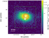 |
Fig. 1. Lyα narrowband surface brightness (SB) image of 4C04.11 derived from the data cube using 6704 − 6710 Å in the observed frame. The blue contour indicates the He II emission region. The contour is calculated from the pseudo-narrowband image of He II using 9028 − 9044 Å in the observed frame with the level of 3σHe II and 2 × 3σHe II, where σHe II is the standard deviation derived from a source-less region of the He II pseudo-narrowband image. The white contour traces the position of the radio jet observed by MERLIN (Multi-Element-Radio-Link-Interferometer-Network; Parijskij et al. 2013, 2014) with the level of 0.45 × (−1, 1, 2, 4, 16, 32, 48) mJy beam−1 following Parijskij et al. (2014). The overlaid red circle with a 1 arcsec radius marks the aperture over which the master spectrum is extracted. The green dashed box shows the FOV of individual panels in Figs. 7 and 8, which is the region we focus on in the spatial mapping in Sect. 5. |
The master spectrum is shown in Fig. 2 with the upper panel focusing on emission lines and lower panel focusing on the continuum. In the figure, we mark the emission lines with significant detection that our analysis will focus on: Lyαλ1216 (hereafter Lyα), C IVλλ1548, 1551 (hereafter C IV), He IIλ1640 (hereafter He II) and O III]λλ1660, 1666 (hereafter O III]). We also mark the low S/N N Vλλ1238, 1243 (hereafter N V). The flux of N V is indistinctly low and highly absorbed. Additionally, its position is located in the Lyα wing making it hard to detect in the full spectrum (Sect. 4.3). Using the black dotted lines, we indicate the potential positions of Si IVλλ1393, 1402 (hereafter Si IV, the overlapped O IV] quintuplet is not shown). We perform the fitting of Si IV following Sect. 3.2, but the S/N is so low that the line model is poorly constrained. Hence, we consider it as an un-detection.
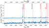 |
Fig. 2. Rest frame UV spectra of 4C04.11. Upper panel: full MUSE spectrum extracted from the central 1 arcsec aperture region. We refer to this spectrum as the master spectrum. The detected UV lines (Lyα, C IV, He II, and O III]) are marked with red dashed lines. We also mark the N V, which has a low S/N, overlaps with the broad Lyα wing, and is not obvious in this full spectrum (see Sect. 4.3). We use the black dotted line to indicate the position of the undetected Si IV. Lower panel: same plot as the upper panel but zoomed in to show the continuum. We note that the skyline residuals are seen as regions with higher noise. The horizontal black dashed line marks the zero flux level. |
3.2. Spectral analysis
We fit models to the observed emission lines to study the physical properties of the gaseous halos of 4C04.11, for example the emitted flux and absorber column density. To do this task properly, we use the Gaussian or Lorentzian model to describe the emission and Voigt-Hjerting function (e.g., Tepper-García 2006, 2007) for the absorption. The fitted function (Eq. (A.8)) is composed of the emission model(s), Fλ, G or Fλ, L (defined as Eq. (A.2)), multiplied with the convolved Voigt function(s) (Eq. (A.7)). The convolution with the MUSE line-spread function is applied to account for the instrumental resolution. The decision whether Gaussian or Lorentzian function is used for modeling the emission components is made based on several reasons explained in Sect. 4. In Appendix A, we explain the definitions and equations used in our fitting. The underlying assumption made when fitting the Voigt profile to the absorption is that each of the absorbing cloud gas has a covering factor close to unity (C ≃ 1.0).
We use different strategies to manage the continua for different lines (see Sect. 4 and Appendix C.1 for details of different lines). The basic idea is to fit the continuum around the emission line with the emission part masked. After the continuum fitting, we then apply the nonlinear least-squares (least-squares for short) algorithm, which preforms with χ2 minimization to fit the interested spectra. Because of the number of free parameters used in the fitting or/and insensitivity of the algorithm to one (or some) of the variables, several problems appear when running the least-squares method, for example the covariance matrix from which uncertainties of the fitting are derived cannot be produced. Then we apply a more sophisticated method, Markov chain Monte Carlo (MCMC; using the python package emcee; Foreman-Mackey et al. 2013), which realizes the fitting through maximizing the likelihood, to better constrain the results and determine the fitting uncertainties. To fulfill this, we perform the MCMC fitting using results from least-squares as initials. We report the results together with the  in Sect. 44.
We note that the reported “1σ” uncertainties in this paper are either the direct reported value of the 1σ confidence level from the algorithm (half the difference between the 15.8 and 84.2 percentiles) or the propagated value from this. Due to the large number of free parameters used in the fitting model and the physically limited parameter ranges, we cannot always explore the entire parameter space, that is to say, the fitting procedure seldom gives us the 3σ confidence level. Hence, we take the compromise to report the 1σ confidence level for a reference. Some of the reported formal uncertainties are too small compared to the instrumental limitations, for example the uncertainty of the line center and the spectral resolution of MUSE.
3.3. Spatial mapping method
The MUSE observations allow us to spatially and spectrally map the gaseous halo around 4C04.11. We mainly focus on the morphology, kinematics and absorption column density distribution of Lyα emission because of its high surface brightness. The spatial properties of C IV absorbers are also studied but only in two spatial apertures due to its relatively low S/N. Hence, we describe here the method we use for mapping the Lyα characteristics in this subsection and show the details of C IV together with its result in Sect. 5.2.
The first step is to spatially bin the data of the Lyα emission region to increase the S/N for the following fitting. We adopt the method from Swinbank et al. (2015), which starts at the brightest spatial pixel (spaxel) and bins the spaxels around it until the set S/N or the number of spaxels in one bin threshold is reached. The S/N threshold is set to be 13, which is close to the median value of the spaxel-based S/N in the region enclosed by the green box shown in Fig. 1 and calculated from the wavelength range 6672 − 6695 Å. This wavelength range is slightly bluer than the peak emission wavelength of Lyα because we are interested in the spatial distribution of the absorbers that are located in the blue wing of Lyα. The largest length of one tessellation bin is 25 spaxels (5 arcsec), which is ∼5 times the size of our seeing disk (Sect. 2.2) to include any large-scale structures with low S/N. The commonly used Voronoi binning (Cappellari & Copin 2003) method is not suitable for our purposes due to the high S/N gradient across the Lyα nebula (∼150 to ∼10 in 20 spaxels). We manually bin some spaxels after running the algorithm to achieve a more homogeneous S/N distribution. There are 64 bins in the final result, which is shown in Fig. F.1.
Next, we fit the Lyα spectrum extracted from each bin following the description in Sect. 3.2, namely we first fit with the least-squares method and then used MCMC to refine the fit. We note that only H I absorbers #1 and #2 (see Sect. 4.1) can be identified in all bins. But for consistency we include all eight absorbers in each fit. To minimize the number of free parameters and keep the fitting of absorbers #3−8 less problematic (especially for those bins where they cannot be seen), we fix the positions (velocity shifts) of these 6 absorbers using the values derived from the aperture-extracted Lyα fitting (see Sect. 4.1). We also fix the continuum fitted from each spectrum prior to including the combined Gaussian plus Voigt profiles in the fitting function. The results are presented in Sect. 5.1.
3.4. Photometry data and SED fitting
4C04.11 has multiband photometry available from previous observations, namely, B, V, R, I and K bands reported in Parijskij et al. (2014), 4 bands of ALLWISE (an extended survey of Wide-field Infrared Survey Explorer; Wright et al. 2010; Mainzer et al. 2011) archival data and Spitzer IRAC 1 and 2 observation (ID 70135, PI: D. Stern see Wylezalek et al. 2013, 2014, for data reduction and flux measurement). In addition, Snios et al. (2020) reported the Chandra 0.5−7 keV X-ray continuum detection of our target. Using these data, we preform a spectral energy distribution (SED) fitting with X-CIGALE (X-ray module for Code Investigating GALaxy Emission; Boquien et al. 2019; Yang et al. 2020, the used photometric data and fitting result are presented in Appendix B) and show the SED fit in the appendix.
We extract the unattenuated stellar emission flux at rest frame 1.6 μm from the fitted SED model from which M⋆ is estimated using the extrapolated IR mass-to-light ratio and galaxy age relation (e.g., Fig. 2 in Seymour et al. 2007). The 1.6 μm is a “sweet spot” for deriving M⋆ of HzRGs. The flux at shorter wavelengths is dominated by young stellar populations (and contaminated by emission lines) and the shape of the SED beyond the stellar emission bump at around 1 − 2 μm is dominated by AGN-heated dust. Hence, the flux at ∼1.6 μm is dominated by the bulk of the stellar population. We consider our stellar mass estimate of M⋆ < 6.9 × 10¹¹ M⊙ as an upper limit due to unaccounted for contributions from AGN-heated dust.
This derived upper limit of the stellar mass is quite high but comparable to other HzRGs (1 < z < 5.2, De Breuck et al. 2010). Therefore, taking into account the derived upper limit and the stellar masses from a large sample, we set the M⋆ of 4C04.11 to ∼2 × 10¹¹ M⊙ and use this value for following calculation. Galaxies with M⋆ ∼ 1011 M⊙ are extremely rare (log(Φ/dex−1/Mpc−3) ∼ 10−6) at the redshift (z = 4.5077) of our object (Davidzon et al. 2017). This indicates that 4C04.11 is a rare galaxy that assembled most of its mass and formed stars when the Universe was very young. It is of great interests to study the different phases of feedback as well as the current environment of such an object.
To estimate the total (baryonic and dark matter) mass of our object, we assume the M⋆/Mhalo ratio to be 0.02 (see Behroozi et al. 2013). This ratio has a large uncertainty, especially for objects at z > 4. For high M⋆ objects at high redshift with extremely low number density, it is difficult to predict from simulation works (e.g., Behroozi et al. 2019). The evolutionary trend from Behroozi et al. (2013) shows that this ratio will be higher in the early Universe for objects that are the progenitors of present day massive galaxies (assumed to be applicable to HzRGs, see Sect. 1). Hence, we adopt a conservative value of 0.02, which is the maximum ratio predicted by Behroozi et al. (2013). Then we can calculate the virial radius of the host galaxy, Rvir ≃ 117 kpc, using

where (1 + z)3 = (1 + z)/3 given by Dekel et al. (2013). This is accurate to a few percent for a system at z ≳ 1.
Using the following equation from the same work,

we also calculate the virial velocity of our target to be ≃583 km s−1. The virial temperature is at the order of 107 K. We note that these should be treated as approximation since we only take the M⋆ derived from the SED fitting as an upper limit and use the maximum predicted M⋆/Mhalo ratio value in calculation.
4. Line fitting results
In this section we present the line fitting results of Lyα, N V, C IV + He II and O III]. We remind the readers that the metal absorbers are not as robustly detected as H I absorbers, which have well-defined trough(s) in the spectra in visual check. This is probably due to the depth of the exposure and the spectral resolution. Hence, during the fit, we assume they are at the similar redshift (velocity shift) to the corresponding H I absorbers. The reasons a subset of the absorbers are considered are presented in corresponding subsections (see Sects. 4.2 and 4.3). We refer them as “detection” if their probability distributions in the corner plots (Appendix E) are well constrained. To visually distinguish the better and poorly constrained absorbers, we use the short solid bars and dashed bars with lighter colors in the figures showing the fitting results, respectively.
We also run a test on fitting the C IV and N V without absorption. The overall shape of the C IV could be fitted without absorbers involved. However, the deep trough around 8500 Å, which is too broad to be influenced by skylines (see Fig. 4), cannot be reproduced. As for N V, the algorithm failed to reproduce the systemic emission component. Hence, we believe the absorbing material is enriched and fit the aforementioned two lines with absorbers.
4.1. Lyα
We use a double-Gaussian model to fit and estimate the un-absorbed emission. We note that Lyα is a resonant line, which makes it difficult to trace the intrinsic velocity range where the photons originated from. The double-Gaussian model used is a simple implementation to fit the high emission peak with a broad wing. This two-component fitting is also applied to the C IV and N V but with different velocity shifts (Sects. 4.2 and 4.3). This indicates there are at least two components of gas emission with different physical origins (further discussion in Sect. 6.1).
We present the best-fit model of Lyα in Fig. 3 upper panel with dark magenta line. In the figure, we mark the positions of eight H I absorbers. The best-fit parameters are presented in Table 1 (for emissions) and Table 2 (for absorption). Figure 3 middle panel shows a NH I sensitivity test for the model of absorber #1. We vary the column density of absorber #1 from 1014 cm−2 to 1017 cm−2 with all other parameters fixed to the best-fit values and find that the profile is only sensitive to the NH I near the best fit value (dark magenta line shown in the figure). This test shows that the column density variation in one absorber has little influence on the others unless it is saturated.
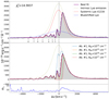 |
Fig. 3. Lyα fitting result and model sensitivity check. Upper panel: best fitting result of the master Lyα line using the MCMC method. The dark magenta line represents the best fit, while the dotted olive line traces the overall Gaussian emission. The systemic emission is shown in a red dotted-dashed line, and the blueshifted emission is marked by a blue dashed line. The positions of all eight absorbers are shown in this panel with black vertical bars. The |

Best absorption fitting results of the 1D aperture-extracted spectrum using the MCMC method.
We include further details on the Lyα fitting procedure in Appendix C.2. The boundary conditions used for the fitting are also presented in Appendix C.2. In Appendix E we show the corner plot (Fig. E.2) and acceptance fraction plot (Fig. E.1), which traces the correlations between each pair of fitted parameters and quality of the MCMC run, respectively.
Humphrey (2019) studied the contamination of O V] λλ1213.8,1218.3 (hereafter O V]) and He IIλ1215.1 emissions for high-redshift Lyα emitters (Type-2 quasars, HzRGs). In general, the contribution from He IIλ1215.1 is insignificant while the O V] emission can contribute 10% (or more) to the Lyα + O V] + He IIλ1215.1 flux if certain ionization parameter and metallicity are given. By using the grid model search, Humphrey (2019) proposed a correlation between O V] and N V, which can be used to estimate the significance of the contamination. To test how O V] will affect the H I fitting result, which is the primary goal of this work, we run the fit of Lyα including the emission doublet of O V]. In this test, the total O V] flux is fixed to 2.5FN V according to Humphrey (2019) with FN V being the total fitted N V flux (Sect. 4.3) in this work. We also fix the FWHM of O V], a nonresonant line, to the value derived from He II (Sect. 4.2). The results of the 8 H I absorbers, especially the NH I, are similar to the fitting results without O V]. Therefore, we do not include the O V] into the Lyα fitting in order to avoid introducing more free parameters.
4.2. C IV and He II
The first line we focus on is HeII, which is the brightest nonresonant line often used for determination of the systemic redshift of HzRGs observed in optical band (e.g., Swinbank et al. 2015; Kolwa et al. 2019). The nonresonant photons are produced through the cascade recombination of He+; they are not energetic enough to induce other transitions and suffer less from scattering than resonant lines (e.g., Lyα). Previous work (Kopylov et al. 2006) determined the redshift of 4C04.11 from the resonant Lyα line, which also heavily suffers from absorption (see Sect. 4.1). Hence, our fitting of the He II will provide a better estimate of the systemic redshift.
C IV and He II are located in the wavelength range that is affected by many strong skylines (Fig. 4, 8200 − 9300 Å, see Hanuschik 2003, for skylines observed at Paranal). Additionally, this wavelength range is near the edge of spectral coverage of MUSE. To obtain better results from these two low S/N lines, we have to reduce the number of free parameters used during the fitting. For this purpose, we (i) fit C IV together with He II and constrain the line center of the systemic C IV component with the redshift determined from He II; (ii) fix the continuum to a first-order polynomial during the emission and absorption fitting; (iii) use a Lorentzian profile for the systemic He II and C IV to avoid an additional Gaussian component; (iv) include only 4 C IV absorbers and fix the Doppler parameters and redshifts of absorber #2 and #3 (further descriptions are presented in Appendix C.3).
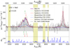 |
Fig. 4. Best fit of the C IV and He II lines from the master spectrum using the MCMC method. We use the dark magenta line to trace the best fit of these two lines. For the intrinsic C IV and He II, the yellow dotted line is used. We mark the systemic emissions of the C IV doublet in dotted green and dashed red lines and blueshifted emissions in dotted and dot-dash blue lines. The |

The best-fit model of He II and C IV are presented in Fig. 4 while fitted parameters are shown in Table 1 and Fig. 4 for emission and absorption (only C IV), respectively. The systemic redshift calculated from the intrinsic He II emission is 4.5077 ± 0.0001, which is a significant improvement compared to Kopylov et al. (2006) (∼10 Å, in observed frame or −1888 km s−1 difference of the He II center wavelength). We detect and report a blueshifted C IV emission component (blue dot-dash and dotted line in Fig. 4) with a relatively high velocity shift of Δv = −1026 ± 112 km s−1. The high blueshifted velocity component is also detected in N V (Sect. 4.3, further discussion in Sect. 6.1). The intrinsic C IV (and He II) emission is shown in thick yellow dotted line from which it is clear that the absorption is needed to describe the line profile, especially the trough around 8500 Å. The standard deviation derived from the data reduction is shown in the lower panel of Fig. 4, which is used as weight in the fitting as well as tracer of the skylines. We excluded several regions (shaded yellow) that are affected heavily by skyline residuals during the fit. We note that there are two regions of skylines (overlap with C IV absorbers #1 and #4) that are already given a low weight during the fit. Hence, we do not mask them in order to avoid complicating the absorption fit.
In Appendix E.2, we present the corner plot (Fig. E.4) and acceptance fraction plot (Fig. E.3) which traces the correlations between each pair of fitted parameters and quality of the MCMC run, respectively. From the corner plot, we notice that C IV absorbers #2 and #3 are loosely constrained. Therefore, we only consider the column densities of absorbers #2 and #3 as upper limits (see Appendices C.3 and E.2 for a further discussion). To visually distinguish them from the better constrained absorbers #1 and #4, we use the dashed bars and lighter colors for absorbers #2 and #3 in Fig. 4.
Nesvadba et al. (2017a) analyzed 4C04.11 with SINFONI observation (the Spectrograph for INtegral Field Observations in the Near Infrared; Eisenhauer et al. 2003; Bonnet et al. 2004) which reported the detection of the [O II]λλ3726, 3729 ([O II]), a nonresonant line, with good S/N (Fig. 11). The redshifts reported by Nesvadba et al. (2017a) based on [O II] fitting are 4.5100 ± 0.0001 and 4.5040 ± 0.0002 for the two narrow Gaussian components used, respectively. Our fitted systemic redshift is in between these two values, which we consider to be reasonable and consistent with the near infrared observation (see Fig. 11). In addition, the authors detect and include a broad blueshifted component (Δv ≃ −240 km s−1, FWHM ≃ 1400 km s−1). We use the Lorentzian profile for the systemic He II because the S/N in this wavelength range of our data is not enough to constrain the fitting with two Gaussian (Appendix C.3). We further discuss this in Sect. 6.1.
The blue wing of He II is too noisy to constrain whether there is a blueshifted component. We present three emission models of the blueshifted He II in Fig. 4 (black dashed, dotted and dash-dotted lines) with velocity shift and FWHM fixed to the blueshifted component of C IV. The line flux of this components are set to be 0.2 (dashed), 0.3 (dotted) and 0.4 (dash-dotted) of the total fitted flux of the blueshifted C IV. From this we can estimate a lower limit of FC IV,b.l./FHe II,b.l. ≳ 3.3. We discuss this result further in Sect. 6.1.
4.3. N V
To fit the low S/N N V on top of the broad wing of Lyα and relatively high continuum, we fix the Lyα to the one derived in Sect. 4.1 and use a constant continuum during the N V fitting. The fitting procedure is then carried out following Sect. 3.2 (see Appendix C.4 for details of the N V fitting).
We show the best-fit N V model in Fig. 5 and the fitted parameters in Tables 1 (emissions) and 2 (absorption). The blueshifted emission component is at ∼ − 1587 km s−1 which is consistent with the C IV blueshifted component5. The large value of Doppler parameter, b ≃ 387 km s−1, could be due to unresolved redshifted H I absorber(s) and/or it is influenced by the skyline subtraction. However, we cannot constrain more without deeper and higher-resolution data. We remind the readers that this fit is limited by the low S/N of the data and depends strongly on the Lyα broad wing and it should be treated with caution. In Fig. 5, the positions of the marginally constrained absorber are shown. Given the degeneracy between b and N (e.g., Silva et al. 2018a), the NN V,1 should be treated as lower limit. The black dashed line in Fig. 5 shows the combined emission structures from all sources (lines and continuum) without absorption. It is clear that at least N V absorber #1 is necessary to fit the data. We note the presence of skylines overlapping with N V (lower panel in Fig. 5), which are already given a low weight in the fitting. Hence, we do not mask them in order to avoid complicating the absorption fitting. We further discuss the interpretation of the emission and absorption results in Sects. 6.1 and 6.3.1, respectively.
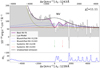 |
Fig. 5. N V best-fit model from MCMC method. The dark magenta line shows the best N V fit combined with the Lyα from Sect. 4.1. The black dashed line marks all combined emissions without absorption. The systemic emissions are marked in dotted green, and dashed red curves show the doublet. The zero velocities of the systemic emissions for the doublet components are derived from the He II result. The blueshifted components are shown in dotted and dot-dash blue lines for the doublet. The solid olive line shows the Lyα model, which is fixed in the N V fit. The short green (red) vertical bars with numbers show the positions of the absorbers on top of the N Vλ1239 (N Vλ1243) line. The dashed line style and lighter color are used to indicate that N V absorber #1 is marginally constrained (see text). The |

In Appendix E.3 we present the corner plot (Fig. E.6) and acceptance fraction plot (Fig. E.5), which traces the correlations between each pair of fitted parameters and quality of the MCMC run, respectively.
4.4. O III]
For 4C04.11, the O III] doublet is detected. Although the O III] is near the He II, we fit them separately in order to avoid introducing more free parameters into the C IV + He II fit, which is one of the major focuses of this work. The fit is preformed following Sect. 3.2 with the line centers and underlying continuum fixed to the systemic redshift implied from He II (Sect. 4.2) and to the model derived in Sect. 4.2, respectively. We present the result of the O III] fitting in Fig. 6 and Table 1. The corner plot and the acceptance rate are shown in Appendix E.4.
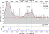 |
Fig. 6. O III] best-fit model using the MCMC method. The dark magenta line shows the best O III] fit combined with the He II from Sect. 4.2. The emissions of the O III] doublet are shown in dotted green and dashed red curves. The line centers of the systemic emissions expected for the doublet components from the He II implied redshift are shown in vertical dotted green and red lines. The solid olive line shows the He II model that is fixed in the O III] fit. The |

5. Spatial mapping
In this section we present the spatial mapping results for Lyα and C IV. The Lyα emission is analyzed by following the method described in Sect. 3.3 and can be studied in detail in both emission and absorption. As mentioned in Sect. 3.3, C IV is detected at low S/N and its quality suffers from skyline contamination. For C IV, we therefore only focus on the results from two larger spatial regions in Sect. 5.2. It is impossible to fit the N V spatially due to its extremely low S/N even in the master spectrum.
5.1. Spatially resolved Lyα signatures
We first present the morphological and kinematic features of Lyα emission derived from the spatially resolved fitting analysis (Fig. 7). In each panel, we show the measured parameters in 64 spatial bins identified through our binning method in Sect. 3.3. In Fig. 7a, we show the intrinsic Lyα surface brightness (SB) map. It is important to note that this shows the integrated Lyα flux derived from the Gaussian emission model (summation of the two components; see Sect. 3.2), after correction for the H I absorption. The extended emission to the north, encompassing the northern jet hotspot, is due to the large size of the bin (see Fig. F.1, bin 59). The position of the SB peak coincides with the radio core (central green contours). In all panels of Figs. 7 and 8, we overplot this intrinsic Lyα SB as black contours. In Fig. 7b, we present the W80 map generated from the unabsorbed Lyα emission. W80 is a nonparametric measurement of the velocity width of emission lines (e.g., Liu et al. 2013). We notice the W80 peaks close to the southern jet hotspot, which is likely the approaching jet because of its clumpier morphology, which in turn could be caused by Doppler beaming (Parijskij et al. 2014). While we consider that result as tentative, it may be a signature of jet-gas interactions (e.g., Humphrey et al. 2006; Nesvadba et al. 2017a). We present the v50 map in Fig. 7c, which is a nonparametric measurement of the velocity shift of the emission profile (e.g., Liu et al. 2013) independent of interpreting the individual Gaussian components added to the fit. The result suggests the existence of blueshifted Lyα emission. However, since the map is based on fitting and estimating the intrinsic, unabsorbed Lyα emission (i.e., it is not fully nonparametric), we do not interpret it further.
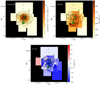 |
Fig. 7. Spatial mapping results of Lyα emission. The contours are the same in all panels, with the green showing the position of the radio source (see the Fig. 1 caption for details; Parijskij et al. 2013, 2014) and black tracing the Lyα surface brightness resulting from spatial fitting (the levels are given arbitrarily). All these maps are constructed based on the fitting results, i.e., not directly from the data. (a) Intrinsic surface brightness map of Lyα emission. (b) W80 map of Lyα emission (nonparametric measurement of the line width; see text). (c) v50 map of the fitted Lyα emission profile (nonparametric measurement of the line-of-sight velocity; see text). |
Figure 8 shows the column density and velocity shift maps for absorbers #1 and #2, which are the two prominent absorbers detected in every spatial bin suggesting high areal fractions. We note that we show here the velocity shift with respect to the mean velocity of the respective absorber Δv as derived from the from the master spectrum (see Table 2). In Fig. 8a, we identify a column density gradient in absorber #1 from southwest (SW) to northeast (NE), which is roughly in the perpendicular direction to the radio jet axis with an increasing of 1 dex in 24 kpc. We consider this as a robust detection after checking the associated uncertainties in each bin. In Fig. 8b, we identify a small velocity gradient for absorber #1 along the direction of the jet increasing from ∼ − 50 km s−1 in the southeast (SE) to ∼35 km s−1 in the northwest (NW) in 20 kpc. In Sect. 7, we discuss possible explanations for these observations.
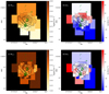 |
Fig. 8. Column density and velocity shift maps of H I absorber #1 (panels a and b) and #2 (panels c and d). The black contours are the same as in Fig. 7. The zero points for the velocity shift maps are chosen individually to be the Δv of each absorber as derived from the master spectrum fitting reported in Table 2. The maps therefore show the velocity shifts relative to the redshift of the respective absorber. |
We do not observe such gradients or spatial variations in the column density and velocity shift maps of absorber #2 in Figs. 8c and d. We note that the fitting uncertainties for absorber #2 are larger compared to those for absorber #1, such that any small variations would not show up in our analysis. This also demonstrates that our observations only provide us with enough sensitivity to study the spatial properties of H I absorber #1. Hence, we do not show the maps for absorbers #3−8. During the analysis of the spatial properties of the C IV absorbers, we also extract and fit the Lyα spectra from the two spatial apertures (see Sect. 5.2 for details) that partly constrain the high-velocity shift of the H I absorbers at different positions. The results of the fitted parameters are presented in Table G.2. Though the S/N is low and some absorbers are only partially constrained, we do not observe any significant changes in column density for absorber #3−8 in the two regions. We notice that we do not observe any strong velocity gradients for any of the absorbers. We therefore exclude the possibility of absorber spatial blending, that is, absorbers identified at the same wavelength position could not be different absorbers in different spatial bins.
In Appendix F, Figs. F.2–F.5, we present the fitting results of 64 individual Lyα spectra from the 64 spatial bins.
5.2. Spatially resolved C IV signatures
We present the spatial analysis of C IV in this section. As mentioned in Sect. 3.3, the S/N of C IV makes it difficult to study its spatial variations in as much detail as Lyα. However, since we observe a column density gradient of H I absorber #1 (Sect. 5.1), it is worthwhile to investigate whether the C IV shows similar features. We manually set two regions from which we extract spectra (Fig. 9): NE where the column density of H I absorber #1 is higher and SW where the column density of H I absorber #1 is lower. When selecting the apertures, we keep the same number of spaxels (30 spaxels or 1.2 arcsec2) in these two regions and avoid the impact of the jet. Most of the spaxels in these two regions are covered in the master aperture (red circle in Fig. 9) in order to be consistent with the 1D spectrum analysis.
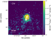 |
Fig. 9. C IV broadband image clasped between 8400 − 8600 Å in the observed frame. The white contour traces the radio jet, while the red circle marks the position where the spectrum analyzed in Sect. 4 is extracted (see the caption of Fig. 1). The dark blue and magenta regions show the apertures from which the spectra used to studied the spatial features of C IV are extracted. The spectrum from the dark blue (magenta) region is marked as NE (SW). |
For the spectral fitting, we follow the similar strategy described in Sects. 3.2 and 4.2. The fitting results from these two regions are presented in Table G.1 for emissions and Table G.2 for absorption. In Fig. 10, we show the best-fit models of the two C IV lines. The intrinsic C IV emission shown in the figure indicates that the absorption is indeed needed to better describe the line profile, especially in the NE. The quality of the C IV fits is affected by their low S/N partly due to smaller aperture from which the spectra are extracted and the influence of skylines. To avoid over-fitting, we fix the Doppler parameters, b, and redshifts, z, of all absorbers in the two regions and refer to the column density results as upper limits. The exception is the column density of C IV absorber #1 in the NE region, which has a well-defined probability distribution and is considered a detection (see Appendix G and Fig. G.1 for more details). In Fig. 10, we mark the positions for the un-constrained absorbers in dashed bars with lighter colors to visually distinguish them from absorber #1 in the NE region.
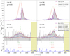 |
Fig. 10. Spectra and fit of Lyα (top row) and C IV (middle row) and noise spectra of C IV (lower row) extracted from the dark blue (NE) and magenta (SW) regions shown in Fig. 9. The positions of H I absorber #1 are marked with black bars in the top row. The velocity shift is relative to the systemic redshift, z = 4.5077, fitted from He II (Sect. 4.2). The line styles used to show the fitting results are the same ones as that of the master Lyα (Fig. 3) and C IV (Fig. 4). We note that except for C IV absorber #1 detected in the NE region, the positions for the other C IV absorbers are marked in dashed bars, with lighter colors indicating that they are only marginally constrained (see text), which is consistent with the “master C IV” presentation (Fig. 4). The intrinsic C IV emission is also shown in orange dotted lines for the two spectra in the middle row. The panels in the bottom row show the standard deviations (noise) of the C IV spectra derived from the variance extension of the data cube, which are used as fitting weights. They are shown in the same units as the data spectra and can be used to show the quality of the spectra and trace the positions of skylines. |
In addition, we extract the Lyα spectra from these two regions and perform the fitting analysis (Fig. 10) with the goal to compare the column density ratio of the C IV and Lyα absorber #1 (results shown in Tables G.1 and G.2). We measure NC IV, NE/NH I, NE = 0.11 ± 0.04, and NC IV, SW/NH I, SW < 0.04 and further interpret this result in Sect. 6.3.2.
We also perform the similar analysis for another two regions along the radio jet for completeness (not shown in Fig. 9). The two regions are chosen to be the similar as the previous dark blue and magenta ones but rotated 90° clockwise with respect to their geometric center. The column density variation in C IV absorber #1 is also tentatively identified along this direction as well as the H I−C IV ratio (SE-NW) with NW region having a higher value. Specifically, the C IV absorber #1 is only marginally fitted in the SE region with its result can only be used as upper limit. We also check the velocity shift of the H I absorber #1 in the two regions (SE-NW) along the radio axis and confirm the gradient observed in Fig. 8.
6. Discussion
6.1. Emission line properties
Emission line fluxes, flux ratios and spatial locations of individual kinematic components provide powerful diagnostics of gas properties and ionization source. In this work, we detect five UV lines, namely Lyα, N V, C IV, He II and O III]. Lyα is a resonant line that suffers heavily from scattering, making it difficult for us to trace its intrinsic velocity structures (e.g., Dijkstra 2014). Although we detect a blueshifted broad component, we refrain from assigning it a physical meaning and do not to compare it with the blueshifted components seen in N V and C IV.
6.1.1. Emission line characteristics
We first compare the emission line properties for Lyα and He II detected with MUSE in this work and the [O II] from SINFONI (Nesvadba et al. 2017a). In Fig. 11, all lines are shown within the velocity range where the zero point is set by the systemic redshift derived from the He II fit. For Lyα and He II, their best fits from this work are shown. In addition, we include the fitted line centers of the narrow component of the [O II] doublet (pink dotted lines) and the broad component (pink dot-dash line) (Nesvadba et al. 2017a), respectively. We note that the wavelength calibration for SINFONI is done using the vacuum wavelength while MUSE uses air wavelengths. To eliminate this discrepancy, we apply the equation from Morton (2000) to convert all wavelengths into air wavelengths6. We did not correct the difference in wavelength due to the heliocentric frame used in SINFONI observation, which is ∼30 km s−1.
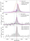 |
Fig. 11. Comparison between the Lyα, He II, and [O II] rest-frame spectra. The Lyα and He II presented here are the same ones analyzed in Sects. 4.1 and 4.2 in velocity scale. We subtract the continuum from the He II here to better present the low flux region of the emission. The black lines are the same ones as shown in Fig. 4 for the blueshifted He II models, with the dashed, dotted, and dash-dotted lines indicating the line flux of 0.2, 0.3, and 0.4 of the total fitted flux of the blueshifted C IV. The [O II] is taken from SINFONI (Nesvadba et al. 2017a). In each panel, the black dashed lines indicate the zero velocity. In the last two panels, the dashed vertical teal blue lines show the velocity shift of the C IV blueshifted component. For Lyα and He II, the best fit models from this work are shown. We also mark the fitted line centers of the [O II] narrow doublet from Nesvadba et al. (2017a) in pink dotted lines and the broad component line center in a pink dash-dot line. |
In the He II panel, we show again the three blueshifted models with the line center fixed to the value obtained from C IV fit as in Fig. 4. The velocity of the C IV blueshifted component is indicated by the vertical dashed blue line in He II and [O II] panels. From this figure, we conclude that the broad blueshifted component observed in [O II] (Δv ≃ −240 km s−1, FWHM ≃ 1400 km s−1) is not seen in He II. Though affected by resonant scattering, the blueshifted Lyα component is consistent with the blueshifted component seen in [O II] and they both may trace emission from the same potential outflow. The high-velocity blueshifted component (as seen in C IV), however, is possibly also present in [O II]. We discuss this in Sect. 6.1.2 together with N V and C IV. The marginally detected continuum in Nesvadba et al. (2017a) is consistent with our MUSE observation.
6.1.2. Emission line ratios and sources of ionization
We next investigate the emission line flux ratios for the individual kinematic components that we observe for N V, C IV, and He II in order to determine the ionization mechanism. In Sect. 4, we report the fitted intrinsic emission line fluxes of these three lines. The derived flux ratios are presented in Table 3. For N V and C IV, the flux ratio between their systemic emission line components is FN V, sys/FC IV, sys = 0.32 ± 0.09 (which is comparable to other HzRGs; e.g., De Breuck et al. 2000). The ratio between the systemic C IV and He II components is FC IV, sys/FHe II = 0.55 ± 0.14.
Line flux ratios and equivalent width.
For the blueshifted components, the velocity shifts (with respect to the zero point set by the systemic He II) of the C IV (−1026 ± 112 km s−1) and N V (∼ − 1587 km s−1) are roughly consistent and we therefore assume that they are tracing the same kinematic component of the gas (more detail on Appendix C.4). The flux ratio between the blueshifted components has a value of FN V,b.l./FC IV,b.l. ≃ 0.7. We do not clearly observe a blueshifted component in He II. This is a somewhat different situation compared to observations in other HzRGs. For example, in MRC 0943–242 (a HzRG in our MUSE+ALMA sample, Kolwa et al. 2019) a blueshifted component is observed in C IV (EC IV = 64.5 eV) and He II but not N V. Nevertheless, in order to constrain its flux, we plot three models of the blueshifted He II with velocity shift and FWHM fixed to the values of blueshifted C IV and having flux 0.2, 0.3 and 0.4 of FC IV,b.l. (Sect. 4.2, Fig. 4). From this, we can set a lower limit of FC IV,b.l./FHe II,b.l. ≳ 3.3.
Feltre et al. (2016) presents emission-line diagnostics at ultraviolet wavelengths of photoionization models of active and inactive galaxies with the aim is to identify new line-ratio diagnostics to discriminate between gas photoionization by AGN and star formation. According to their models (Figs. 5 and 7 in Feltre et al. 2016) the ionization source for the systemic kinematic component that we observe in N V, C IV and He II (Table 3) is consistent with photoionization from an AGN, though the C III] data are unavailable. This is also consistent with the diagnostic from Nakajima et al. (2018), which involves the equivalent width of C IV (EW(C IVsys)≃12 Å) and FC IV/FHe II. As for the ionization source of the blueshifted component, the diagnostic from Feltre et al. (2016) indicate it to be due to star formation only with our derived upper limit of FC IV,b.l./FHe II,b.l.. Using EW(C IVb.l.) ≃ 26 Å and FC IV,b.l./FHe II,b.l. ≳ 3.3 and comparing to Fig. 11 in Nakajima et al. (2018), the diagnostics are consistent with the region where ionization from both AGN and star formation are possible. This is surprising given even extreme star formation processes are unlikely to drive such a high-velocity outflow (see Heckman et al. 2015).
High-velocity shocks (due to the radio jets) may be another possible solution to explain the blueshifted emission line component. Dopita & Sutherland (1995, 1996) modeled the shock ionization process and provided spectral line diagnostics that can be applied to narrow line regions (NLRs) of AGN. De Breuck et al. (2000), Humphrey et al. (2008b) used these models to analyze samples of HzRGs and suggested some limitations of these models. Allen et al. (2008) extended the Dopita & Sutherland (1995, 1996) models to embrace larger parameter ranges. Due to the limited number of available spectral lines for 4C04.11 (e.g., lacking useful diagnostic lines [O III]λλ4959, 5007, C III]λλ1906, 1908 and C II]λ2326), we cannot draw strong conclusions on shock ionization scenarios. Nevertheless, with the inferred high FC IV,b.l./FHe II,b.l. and FN V,b.l./FHe II,b.l. (Table 3), the blueshifted emission is not inconsistent with being due to shocks. This is also consistent with [O II] if the flux excess seen at ∼ − 1000 km s−1 (Fig. 11) comes from the same gaseous component with C IV and N V.
We remind the reader that the uncertainties associated with our flux and flux ratio measurements are non-negligible and deeper data are needed to investigate the true nature of the individual gaseous components. Our observations nevertheless indicate that the blueshifted kinematic component observed in N V and C IV traces a metal-enriched (see Sect. 6.3) gaseous outflow within the ISM of 4C04.11 that is distinct in both kinematics and ionization mechanism from the systemic component.
We further investigate the differences between the blueshifted- and systemic components by assessing their respective spatial locations. Usually, the broad component will have compact (often un-resolved) spatial distribution if it is AGN-driven. We compare the spatial locations of these two components from pseudo-narrowband images of C IV focused on its blue wing (8400−8500 Å, −4464 < Δv < −948 km s−1) and on its red wing (8500−8600 Å, −948 < Δv < 2567 km s−1), respectively. The S/N of the N V is too low to preform this check. We do not observe a significant spatial difference as the two components are located around the center of the Lyα SB peak with a extension of ∼3 arcsec (∼2 for the blue wing), which is larger than the seeing element. The large detected line widths of the blueshifted components (Table 1) could also represent a set of individual clouds that are not spatially nor spectrally resolved in our data leaving the possibility open for the AGN being the primary ionization source.
6.2. H I absorbers
When fitting the absorption features in Sect. 3.2, we work with the assumption where several extended screens of gas are responsible for the absorption troughs. This assumption is justified as we coherently observe the signatures of H I absorbers #1, 2, 3, and 4 across large spatial scales, which indicates large areal fractions. The spatial extent for absorbers #1 and 2 is ∼30 × 30 kpc2 (Fig. 8) and ∼16 × 16 kpc2 for #3 and 4 whose maps are not shown in this paper due to their low S/N. For clarification, the presence of absorber #3 and 4 (and further) cannot be obviously identified in the tessellation bins 50−64 (see Figs. F.1–F.5) based on which their spatial extent is determined. The screens may be part of a shell similar to the shell models proposed by many theoretical works, for example Verhamme et al. (2006) and Gronke et al. (2015). For absorber #1, with the highest S/N in our data, we furthermore observe a significant column density and velocity gradient (Sect. 5.1), which we discuss separately in Sect. 7. However, our observations are not sensitive enough to probe the spatial (morphological and kinematic) details of absorber #2 (Sect. 7) or any of the higher-velocity absorbers.
As for absorbers #5−8 (which have velocity shifts with respect to the systemic redshift of −1791 ± 9, −2306 ± 10, −2748 ± 13 and −3348 ± 15 km s−1, respectively), their spatial distributions are difficult to identify since they are located in the blue, low S/N wing of Lyα and are therefore only observed in the high surface brightness regions of Lyα close to the center of the host galaxy. They may have a larger spatial extent but this cannot be constrained without deeper observations. Additionally, we note that there is a large velocity shift difference between H I absorber #4 and #5, ∼600 km s−1. Absorbers #5−8 are therefore likely intervening absorbers between the radio galaxy and the observer beyond the galaxy potential well. The reason that many of these intervening absorbers have large b values when compared to related works about Lyα forest absorption (e.g., Rauch 1998; Schaye et al. 2000; Fechner & Reimers 2007) is probably due to the spectral resolution of MUSE not resolving individual components of connect narrower absorbers (e.g., van Ojik et al. 1997; Jarvis et al. 2003).
If the velocity shift for absorbers #2−4 corresponded to a cosmological redshift difference as is probably the case for absorbers #5−8, we can calculate the physical separation between central radio galaxy and the absorber. For absorber #2, which has the smallest shift, the luminosity distance difference between it and the systemic redshift is 84 Mpc, much larger than the virial radius of the host galaxy, Rvir ≃ 175 kpc (Sect. 3.4). Hence, if the physical distance was the reason for the velocity shifts, all absorbers would be gravitationally unbound to the host galaxy. In contrast, if the velocity shift was caused by the kinematics of an outflowing shell, the absorption troughs can and should be observed on large spatial scales, which they are. Given the velocity offset of absorbers #2, 3, and 4 derived from the master spectrum and their spatial extent (i.e., large areal fraction), we therefore conclude that they are likely outflowing gas shells potentially driven by the AGN.
While the other absorbers (#5−8) are very likely intervening absorbers, we cannot fully exclude from our data that they may represent fast-outflows. For example, Kriss et al. (2018) investigates ultrafast X-ray outflows (UFOs) seen in AGN in absorption and their relation with the associated H I and other lower-ionization ions, such as C IV. These UFOs with vout ≳ 0.1c, where c is the speed of light, are much more extreme cases of outflows compared to our observations. Absorber #8, if it was an outflow, would have a velocity of 0.01c. In addition, the H I absorption widths predicted by the UFOs are much wider than our observations (FWHM ∼ 1000 km s−1), their column densities are lower (< 1014 cm−2) and the required ionization parameter is higher (e.g., compared to absorption studies in other HzRGs; Kolwa et al. 2019). All this indicates that the UFOs seen in X-ray and Lyα absorption studied by Kriss et al. (2018) trace a different scenario than the absorbers in 4C04.11. Even if there was UFO-associated H I absorption for 4C04.11, it would be located at much shorter wavelengths where the continuum level is too faint to allow them to be detected.
6.3. Metal absorption
6.3.1. Metal absorbers in the master spectrum
Relative column density ratios between different elements can provide information on the enrichment of the gas assuming an ionization parameter. The underlying assumption for the metal absorbers analyzed here is that they are ionized by the central AGN (e.g., Kolwa et al. 2019). Constraining whether this AGN photoionization is geometrically possible is beyond the scope of this work given the resolution of the data and the limited knowledge of the evolution state and ionization episode of the radio galaxy. Hence, we do not discuss more about the source(s) of ionization for the metal absorbers and proceed with the discussion of the following implication with the assumption of central AGN ionization. One hint on the AGN ionization could be due to the wide ionization cone that covers some fraction of the absorbing gas seen (e.g., Fig. 12). Nevertheless, we remind the reader that the shocks or a hard source of ionization (for example, AGN of meta-galactic background) inferred by the presence of a high column density N V absorber (see blow) could also be possible.
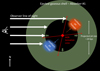 |
Fig. 12. Schematic view of the proposed outflowing shell model in Sect. 7.1. The large dark green annulus represents the outflowing gaseous shell that could be the absorbing cloud of absorber #1. The blue and orange regions mark the southern (approaching) and northern (receding) jet hotspot interacting with the previous ejected shell, respectively. We note that the morphology of the gaseous shell is not necessarily in a circular shell as shown here, and we do not have information for the shell at the backside of the AGN. The red lines in the annulus center indicate the region of the AGN ionization cone that could have a wider opening angle than the jet beam (see text). The column density gradient we observed in Sect. 5.1 in the S-N (SW-NE, due to the orientation on the sky plane, which is not shown here) direction could simply be explained by the different lengths of the observer line of sight intersecting with the gaseous shell at different spatial locations (see text). This process is shown with the length of white arrows intersecting with the dark green annulus in the figure. For the column density decreasing after passing the midplane, which cannot be explained by the geometry setting, the southern jet (blue region) interaction with the ejected gaseous shell could cause the decreasing of column density through instabilities and/or partially ionizing the gas. Though the rough projection size of the jet is shown, we note that other parts of this sketch are not to scale. |
In this work, we identified the absorbers around the systemic redshift of H I, C IV, and N V in the master spectrum, which we sassume belong to the same cloud. The corresponding ratios are NC IV,1/NH I,1 = 0.12 ± 0.05 and NN V,1/NH I,1 = 1.4 ± 0.2. We remind the readers that the NN V,1 should be treated as a lower limit given that the Doppler parameter associated with it hits the upper boundary (Appendix C.4). Comparing this with CLOUDY (spectral synthesis code, Ferland et al. 2017) models (the same models as Fig. 17 in Kolwa et al. 2019), we can roughly estimate that absorber #1 has (super) solar metallicity (Z ≳ 1 Z⊙) independent of a specific assumption for the ionization parameter. The derived NN V,1 value is consistent with the conclusion. This suggests strongly that absorber #1 has an origin inside the ISM of the radio galaxy. Given the age of the Universe at z = 4.5077, it is unlikely that absorber #1 is the infalling material that has been enriched by a previous outflow and is now recycled through a galactic fountain mechanism. The column density, NN V ∼ 14.99 cm−2, is relatively high. As discussed in Kolwa et al. (2019), the secondary nitrogen production is responsible for the nitrogen column density enhancement of the absorber if the gas has (super) solar metallicity (also Hamann & Ferland 1993). Hence, though the CNO cycle for the secondary carbon and nitrogen can produce solar N/C ratio over a large range in metallicities (e.g., Nicholls et al. 2017), Z ≳ 1 Z⊙ is needed, which is consistent with our conclusion here. We further discuss the nature of absorber #1 in Sect. 7 combining the metallicity and spatial features observed in H I.
For absorber #2 and #3, their column density results can only be treated as upper limits. The corresponding ratios of H I absorbers are NC IV,2/NH I,2 ∼ 3 × 10⁻⁴ and NC IV3/NH I,3 ∼ 0.02. In addition, absorber #4 has the ratio of NC IV4/NH I,4 = 0.25 ± 0.05. It is difficult to confine the metallicities of these three absorbers without the data from N V. Nevertheless, the ratios are indicative of the absorbers having sub-solar metallicity according to the CLOUDY models (Z ≲ 0.5 Z⊙), except for absorber #4, which could have solar metallicity. From the discussion in Sect. 6.2, we consider these three absorbers as outflowing gaseous clouds with the one having the highest velocity shift (absorber #4) being the most recently ejected. Combined with the proposed scenario of absorber #1 in Sect. 7.1, the low metallicity of absorbers #2−#4 can be explained: Absorber #1 was ejected first and carried most of the metal elements produced in the early star formation activities. The timescale between the ejection of absorber #1 and the later ejected clouds (absorbers #2−#4) was then not large enough to enrich the gas again to solar like metallicity. If we take it further that this may explain the latest absorber #4 has higher metallicity than absorber #2 and #3 because it has the longest time to be enriched, though this is impossible to be proved and has large uncertainties.
The reason we do not observe C IV absorber#5−#8 could be that they are located in the low S/N emission wing. Considering the discussion in Sect. 6.2, however, this could be alternatively explained as they are intervening absorbers outside the potential well of the central radio galaxy (IGM) and they consist of cold, un-enriched pristine gas.
6.3.2. Spatial distribution
As derived in Sect. 5.2, the column density ratios between the H I and C IV absorber #1 are 0.11 ± 0.04 and < 0.04 for the NC IV, NE/NH I, NE in the NE and NC IV, SW/NH I, SW in the SW, respectively. This is considered to be consistent with the observed H I column density in absorber #1. We compare these two ratios with the CLOUDY models and find that, despite the lack of spatial information of N V, the NE cloud may have solar metallicity (ZNE ≳ 0.5 Z⊙), while the metallicity of the SW cloud may be sub-solar (ZSW ≲ 1.0 Z⊙). Readers should bear in mind that the inferred metallicity of absorber #1 in these two regions are derived from low S/N spectra and should be treated with caution.
If we assume these two regions have similar metallicity, this is consistent with the analysis in Sects. 6.3.1 and 7.1 that absorber #1 is an outflowing shell that is enriched homogeneously by star formation activities in the ISM prior to the launch of the outflow.
On the other hand, if we assume the NE region has higher metallicity than the SW region, it suggests a spatially inhomogeneous enrichment. This could indicate merger activities or unevenly dilution due to cosmic accretion of metal-poor gas. Given that the S/N of the two C IV spectra (especially the SW one), we do not further interpret the result.
7. Large-scale characteristics of H I absorber #1
In this section we discuss several possible explanations for the observed properties (areal fraction, kinematics, column density gradient) of the H I absorber #1 (Sect. 5.1). The H I absorbers #1 and 2 are the only two absorbers in our analysis with a high enough S/N to perform the spatial analysis. We identify a significant column density gradient of absorber #1, but not for absorber #2 (Fig. 8) suggesting a relatively uniform distribution within the uncertainties of our fitting analysis. The data quality does not allow us to spatially map any of the higher-velocity absorbers and we briefly discuss their potential nature in Sect. 6.2. We argue that the absorbing gas responsible for absorber #1 is spatially detached from the Lyα emitting gas since we do not observe any similarity between the kinematics of the absorbing and emitting components (Figs. 7b, c, and 8b). The opposite situation may be seen in the blue absorber in TN J1338–1942 (a HzRG in our ALMA-MUSE sample) where the velocity shift maps of the emission and absorption show resemblance (Fig. 4 in Swinbank et al. 2015) and indicate that emitting and absorbing gas are mixed.
Recently, Gronke et al. (2016, 2017) showed simulations of Lyα radiative transfer through a medium where detailed subparsec structures are considered, which is a more realistic model than a continuous shell model. It should be noticed that our spatial mapping of the column density of H I absorber #1 is far from sensitive enough to probe the details in the absorption medium. In addition, Gronke et al. (2017) concluded that the resultant spectral features of their clumpy model are similar to a shell model, that is, the observational features are not affected much by the absorbing medium being either clumpy or a continuous shell. Hence, we only present simple explanations to the reported column density and velocity gradient (Fig. 8) and use the simulation works to assess them to first-order, leaving sophisticated modeling for future works. For example, Peeples et al. (2019) simulated the CGM on a sub-kiloparsec scale and find that the absorbing gas responsible for observed feature around several hundreds of km s−1 in velocity shift range may span hundreds of kiloparsecs in space. It is impossible even for the state-of-the-art instrument like MUSE to probe the real morphology of the CGM gas given that we can only observe features in projection.
7.1. Outflowing shell
We first consider the model of an outflowing gas shell to explain the column density and velocity shift gradient we identify for H I absorber #1. We remind the reader that absorber #1 is at ∼0 km s−1 and covers a large area of the sky (Sects. 4.1 and 5.1) approximately on scales of 30 × 30 kpc2. We identify a column density gradient along the SW-NE direction increasing over 1 dex in 24 kpc. We also check Lyα spectra extracted from the two spatial regions along the radio jet in the SE-NW direction (the two regions for completeness study of C IV spatial mapping in Sect. 5.2) where we also marginally identify the column density gradient.
Following Binette et al. (2000, 2006), Krause (2002, 2005), we propose that the absorbing material of absorber #1 is a wind-driven gaseous shell. The wind may have been powered by stellar feedback and/or AGN activity several tens of megayears before the radio jet was launched. The wind traveled isotropically with its speed decreasing from thousands of km s−1 within 1 kpc to a few km s−1 at 10 s of kpc (may even halt or fall back; Krause 2005; Wagner et al. 2013; Richings & Faucher-Giguère 2018). Tens of megayears after the beginning of the shell expansion, the relativistic jet is launched. The jet that travels at a few tenths of the speed of light catches up with the previously ejected shell in a few megayears (Parijskij et al. 2014), accelerates and disturbs it. The age of the jet could be even smaller (∼1 Myr) in the scenario described here if an earlier galactic wind has cleared the surrounding leading to fewer interactions of the jet traveling inside the wind-driven shell. The velocity gradient along the radio axis we see in Fig. 8b could be a hint for this jet gas interaction. Using polarization measurements, Parijskij et al. (2014) reported that the southern (northern) jet is very likely the approaching (receding) one, which agrees with absorber #1 velocity shift map (the southern part of absorber #1 is the blue-shifted part). In Fig. 12, we show a schematic presentation of the proposed scenario where the SW-NE column density gradient may be explained by the spatially different intersected length between the observational line of sight (thick white arrows on the left of the figure) and the gaseous shell (absorber #1, dark green annulus). This is a similar situation to the sunlight traveling a longer path through the Earth’s atmosphere when the altitude of the Sun is low and causing more scattering. For the column density decreasing in the northern half of the shell, the gradient may be explained by this geometry. The southern jet, which we believe is the approaching one, may be responsible for the observed column density keeping decreasing in the southern half of the gaseous shell. The approaching and receding jet-gas interaction hotspots are marked in Fig. 12 as blue and red regions, respectively. As the figure shows, the approaching jet catches and disturbs the gaseous shell probably through Kelvin–Helmholtz instability in its surrounding (e.g., Mukherjee et al. 2020). The interaction will cause a decrease in the particle number density (Mukherjee et al. 2020) in the immediate vicinity of the jet hotspot (or the jet may even ionize a part of the cooled gas). Hence, the combination of the two aforementioned effects will result in the observed column density and velocity gradient. Though we mark the approximate projected size of the observed jet, readers should bare in mind that the Fig. 12 is not to scale. We note that the red lines mark the regions of the AGN ionization cones as the radio jets are narrow collimated streams (i.e., opening angles; e.g., Drouart et al. 2012; Obied et al. 2016) of the ionization cones are suggested to be wider than the jet beams. Besides, the jet-gas interaction hotspots are smaller regions compared to the gaseous shell; nevertheless, we emphasize them in Fig. 12 with larger symbols.
Several simulation works have shown the possibility of AGN wind expelling medium to kiloparsec scales (e.g., Wagner et al. 2013, for an AGN driven wind accelerating the surrounding medium to ∼1000 km s−1 within 1 kpc). Oppenheimer et al. (2020) specifically studied the impact of AGN feedback on the CGM. This research shows that feedback can drive out the metal elements, which could explain the metal-enrichment of absorber #1 in our observations. The authors reported that the expulsion of metal elements beyond the virial radius, for example like C IV in our case, takes longer with a timescale of 0.5−2.5 Gyr. Hence, on smaller timescales, such as a few hundred megayears, the CGM can be enriched with the gaseous metal-enriched cloud still within the galactic potential well like the case of 4C04.11. Furthermore, Richings & Faucher-Giguère (2018) showed that swept up gas can efficiently cool within an outflow, which could be one possible origin for the neutral gas that absorber #1 consists of.
In Sect. 6.3 we discussed the enrichment of absorber #1, which is also observed in N V and C IV, suggesting that the absorbing cloud has super solar metallicity. This supports the proposed scenario in which the outflowing shell is launched from within the galaxy where the gas has been enriched through star formation activities. It furthermore suggests that we are observing the redistribution of metals through feedback processes and the enrichment of both the ISM and the CGM. Our previous analysis in Sect. 6.3 is based on the assumption that the metal absorbers (N V and C IV) are ionized by the AGN. This could be possible if the opening angle of the ionization cone is wide enough to cover some fraction of the absorber #1 gaseous shell (like the scenario shown in Fig. 12).
It may be too coincident for absorber #1 to be at Δv ∼ 0 km s−1. Even considering the reported 1σ fitting uncertainty, the range of the velocity shift is still close to 0. We notice that the spectral resolution of MUSE, ∼100 km s−1, is much larger than the MCMC reported probability distribution range. Hence, the absorption could have some intrinsic velocity with respect to the systemic redshift of the radio galaxy, which would need to be verified with high-resolution spectroscopy.
7.2. Absorption by large-scale CGM gas
Peeples et al. (2019) showed the simulation of the FOGGIE project (Figuring Out Gas & Galaxies in Enzo), which focuses on the CGM. In their work, the authors presented the absorption characteristics of the CGM gas on scales of hundreds of kiloparsecs with considerable column density for both H I and metals (for example, C IV). An alternative scenario for the characteristics of our absorber #1 is therefore that it consists of gas in the CGM, which extends tens to hundreds of kiloparsecs and has a complex sub-structure beyond the detectability of MUSE. This gaseous cloud is the surrounding medium unrelated to the ejected material by the central radio galaxy. In this scenario, the column density gradient could be due the uneven concentration nature of the CGM gas as shown in Peeples et al. (2019). The tentative velocity gradient may be invoked through a rotation of the large-scale medium. For a system of virial mass on the order of 1013 M⊙, the virial velocity is around 500 km s−1 (Sect. 3.4), which is larger than the value we observe. While unlikely, this inconsistency between the observed velocity gradient (−50 km s−1 to 35 km s−1, Fig. 8b) of absorber #1 and the virial velocity could be due to a combination of the MUSE spectral resolution and projection effects.
This gaseous halo could be on its way to being accreted onto the central galaxy to feed the SMBH and/or star formation activities. The observed radio jet with a projection length of ∼20 kpc (Parijskij et al. 2014) could be well within the giant CGM gas halo and unrelated if the aforementioned scenario is the case. The high column density part in the north may be related be the inner part of inflow, which is denser according to the simulation presented by Mandelker et al. (2020). The spatial extent of this inflow could be up to ∼60 kpc in our case, which covers the detected absorber #1 well (0.5 Rvir; see Sect. 3.4; Mandelker et al. 2020).
Although this scenario can explain the H I column density and the surrounding medium can be enriched to a small extent, it is difficult to reconcile super solar metallicty with this scenario (Sect. 6.3.1, and especially the high column density of N V). Hence, we consider the model proposed in Sect. 7.1 as the more probable situation.
7.3. Alternative models
Alternatively, the double-peak structure of the Lyα spectrum (which we believe is due to the H I absorber #1) with the trough at ∼0 km s−1 could be explained by other numerical models.
The absorbing gas could be entrained within the jet and detached from the jet path, which could explain the tentative velocity gradient. After the detachment, the gas will gradually slow down, which could explain its low velocity shift around 0 km s−1. This model, however, has problems to reproduce the observed column density gradient in the direction roughly perpendicular to the radio jet.
The absorbing H I gas we see may be the product of the “positive feedback” from the jet interaction with the ISM/CGM (e.g., Croft et al. 2006; Gaibler et al. 2012; Fragile et al. 2017). In this situation, we could ignore the self-gravity of the gas due to the dark matter dominated potential (Fragile et al. 2017), which could explain the velocity shift of around 0 km s−1 of the H I absorber. The jet compresses the CGM gas on its path. The higher H I absorber #1 column density in the NE could be that the line of sight passing longer length in the northern part given the jet orientation (similar to the geometric effect proposed in the outflowing model, Sect. 7.1). This could also in principle explain the observed tentative velocity shift gradient. This explanation again, however, has the shortcoming to reproduce the metal enrichment of absorber #1.
8. Conclusions
In this paper we present MUSE observations of the CGM of a radio galaxy, 4C04.11, at z = 4.5077. Particularly, we focus on the absorption in the halo and its spatial properties. The main conclusions of this work are summarized as follows:
-
The Lyα emission halo is detected on scales of 70 × 30 kpc2 (more extended low surface brightness regions are not shown in the presented narrowband image in Fig. 1). We model the Lyα profile using a double Gaussian and report on a blueshifted component at ∼ − 102 km s−1 whose nature is still debatable. The map of the Lyα velocity width (Fig. 7) may indicate signatures of jet-gas interactions.
-
The systemic redshift of 4C04.11 is derived from the brightest nonresonant line, He II, of 4.5077 ± 0.0001. This is consistent with the near-infrared observation of [O II] (Nesvadba et al. 2017a) and a large improvement compared to previous work using Lyα (Kopylov et al. 2006).
-
Metal emission lines, C IV, N V, and O III] are also detected; C IV in particular can be spatially mapped (Fig. 9). This suggests that the CGM is largely metal enriched. Both the C IV and N V lines show blueshifted emission components with consistent velocity shifts (ΔvC IV,b.l. = −1026 ± 112 km s−1 and ΔvN V,b.l. ∼ −1587 km s−1). This component may have a different ionization mechanism than the systemic emission and could provide evidence for a star formation and/or AGN-driven outflow (Sect. 6.1).
-
We identify at least eight H I absorbers with a velocity shift range of −3345 − 0 km s−1. The column density of these eight H I absorbers are around 1014.8 cm−2, and their Doppler parameters, b, have a range of 40 − 271 km s−1 (Table 2). We infer the presence of two C IV absorbers, which are believed to be associated with H I absorbers #1 and #4 and have a column density of ∼1014 cm−2. The column densities of C IV absorbers #2 and #3 are only constrained to upper limits (Table 2). The presence of absorber #1 is also inferred in N V with a relatively high column density, ∼1014.99 cm−1. This suggests that the first four absorbers are within the potential well of the host galaxy, while absorbers #5−8 are likely intervening absorbers (Sects. 6.2 and 6.3).
-
We spatially map the H I absorbers and identify a column density gradient of absorber #1 in the SW-NE direction (increases 1 dex in 24 kpc; Fig. 8). The velocity map of H I absorber #1 shows a tentative gradient along the radio jet axis, with the blueshifted part in the south. This is spatially coincident with the approaching radio jet (Parijskij et al. 2014). Absorber #1 is also detected in C IV; we can measure its column density in two distinct regions, and we identify a column density gradient similar to that of H I #1, albeit with large uncertainties (Sect. 5.2). We propose and discuss several possible models to explain the observed features. We conclude that absorber #1 likely represents a metal-enriched expelled gaseous shell that is disturbed by the jet that was launched later (Sect. 7.1).
-
Our observations suggest that we are observing the redistribution of metals through feedback processes and the enrichment of both the ISM and the CGM.
This work represents a pilot study and showcases the power of IFS instruments like MUSE for studying the absorbing “invisible” CGM gas and its enrichment and interplay with AGN and star formation activity in and around massive active galaxies in the early Universe. We will perform a similar analysis to our full sample of eight HzRGs with redshift 2.9−4.5, whose SFRs span a wide range (84 − 626 M⊙ yr−1; Falkendal et al. 2019). Although our targets are rare in terms of number density predicted from the galaxy mass function, they are unique representatives for studying the early stellar mass assembly, the feedback process, and the baryon cycle.
This is also the position of the flux peak for Lyα narrowband image collapsed between larger wavelength range (e.g., 6573 − 6819 Å covering the entire Lyα line emission) and white light image of 4C04.11.

Though this reported velocity shift is bluer than the one of C IV blueshifted component taking uncertainty into account, the value of ∼ − 1500 km s−1 will also give C IV a good fit. See Appendix C.4 for more details.
Acknowledgments
We thank the anonymous referee for the valuable comments, which improved this manuscript. All of the MUSE data used in this paper are available through the ESO science archive. This work was based on a Master Thesis supervised by Benjamin P. Moster. We thank his support for the thesis work. We thank Dr. Thorsten Tepper García for pointing us to their erratum and sharing the original numerical code of Voigt Hjerting function. DW is supported by through the Emmy Noether Programme of the German Research Foundation. AH was supported by Fundção para a Ciência e a Tecnologia (FCT) through the research grants UIDB/04434/2020 and UIDP/04434/2020, and an FCT-CAPES Transnational Cooperation Project “Parceria Estratégica em Astrofísica Portugal-Brasil”. MVM acknowledges support from grant PGC2018-094671-BI00 (MCIU/AEI/FEDER,UE). Her work was done under project No. MDM-2017-0737 Unidad de Excelencia “María de Maeztu” Centro de Astrobiología (CSIC-INTA). This work uses the NASA’s Astrophysics Data System and a number of open source software other than the aforementioned ones such as Jupyter notebook (Kluyver et al. 2016); matplotlib (Hunter 2007); SciPy (Virtanen et al. 2020); NumPy (Harris et al. 2020); Astropy (Astropy Collaboration 2018); and LMFIT (Newville et al. 2016).
References
- Adelberger, K. L., Steidel, C. C., Shapley, A. E., & Pettini, M. 2003, ApJ, 584, 45 [NASA ADS] [CrossRef] [Google Scholar]
- Allen, M. G., Groves, B. A., Dopita, M. A., Sutherland, R. S., & Kewley, L. J. 2008, ApJS, 178, 20 [Google Scholar]
- Arrigoni Battaia, F., Prochaska, J. X., Hennawi, J. F., et al. 2018, MNRAS, 473, 3907 [NASA ADS] [CrossRef] [Google Scholar]
- Arrigoni Battaia, F., Hennawi, J. F., Prochaska, J. X., et al. 2019, MNRAS, 482, 3162 [NASA ADS] [CrossRef] [Google Scholar]
- Astropy Collaboration (Price-Whelan, A. M., et al.) 2018, AJ, 156, 123 [Google Scholar]
- Bacon, R., Accardo, M., Adjali, L., et al. 2010, in Ground-based and Airborne Instrumentation for Astronomy III, eds. I. S. McLean, S. K. Ramsay, & H. Takami (SPIE), Int. Soc. Opt. Photon., 7735, 131 [Google Scholar]
- Bacon, R., Vernet, J., Borisova, E., et al. 2014, The Messenger, 157, 13 [NASA ADS] [Google Scholar]
- Bacon, R., Piqueras, L., Conseil, S., Richard, J., & Shepherd, M. 2016, Astrophysics Source Code Library [record ascl:1611.003] [Google Scholar]
- Behroozi, P. S., Wechsler, R. H., & Conroy, C. 2013, ApJ, 770, 57 [NASA ADS] [CrossRef] [Google Scholar]
- Behroozi, P., Wechsler, R. H., Hearin, A. P., & Conroy, C. 2019, MNRAS, 488, 3143 [NASA ADS] [CrossRef] [Google Scholar]
- Bessell, M. S. 1990, PASP, 102, 1181 [NASA ADS] [CrossRef] [Google Scholar]
- Binette, L., Kurk, J. D., Villar-Martín, M., & Röttgering, H. J. A. 2000, A&A, 356, 23 [NASA ADS] [Google Scholar]
- Binette, L., Wilman, R. J., Villar-Martín, M., et al. 2006, A&A, 459, 31 [NASA ADS] [CrossRef] [EDP Sciences] [Google Scholar]
- Bolmer, J., Ledoux, C., Wiseman, P., et al. 2019, A&A, 623, A43 [NASA ADS] [CrossRef] [EDP Sciences] [Google Scholar]
- Bonnet, H., Abuter, R., Baker, A., et al. 2004, The Messenger, 117, 17 [NASA ADS] [Google Scholar]
- Boquien, M., Burgarella, D., Roehlly, Y., et al. 2019, A&A, 622, A103 [NASA ADS] [CrossRef] [EDP Sciences] [Google Scholar]
- Bordoloi, R., Tumlinson, J., Werk, J. K., et al. 2014, ApJ, 796, 136 [NASA ADS] [CrossRef] [Google Scholar]
- Borthakur, S., Heckman, T., Tumlinson, J., et al. 2015, ApJ, 813, 46 [NASA ADS] [CrossRef] [Google Scholar]
- Cai, Z., Fan, X., Yang, Y., et al. 2017, ApJ, 837, 71 [NASA ADS] [CrossRef] [Google Scholar]
- Cai, Z., Cantalupo, S., Prochaska, J. X., et al. 2019, ApJS, 245, 23 [Google Scholar]
- Cantalupo, S., Arrigoni-Battaia, F., Prochaska, J. X., Hennawi, J. F., & Madau, P. 2014, Nature, 506, 63 [Google Scholar]
- Cappellari, M., & Copin, Y. 2003, MNRAS, 342, 345 [Google Scholar]
- Cashman, F. H., Kulkarni, V. P., Kisielius, R., Ferland, G. J., & Bogdanovich, P. 2017, ApJS, 230, 8 [NASA ADS] [CrossRef] [Google Scholar]
- Collet, C., Nesvadba, N. P. H., De Breuck, C., et al. 2015, A&A, 579, A89 [NASA ADS] [CrossRef] [EDP Sciences] [Google Scholar]
- Collet, C., Nesvadba, N. P. H., De Breuck, C., et al. 2016, A&A, 586, A152 [NASA ADS] [CrossRef] [EDP Sciences] [Google Scholar]
- Croft, S., van Breugel, W., de Vries, W., et al. 2006, ApJ, 647, 1040 [NASA ADS] [CrossRef] [Google Scholar]
- Davidzon, I., Ilbert, O., Laigle, C., et al. 2017, A&A, 605, A70 [NASA ADS] [CrossRef] [EDP Sciences] [Google Scholar]
- De Breuck, C., Röttgering, H., Miley, G., van Breugel, W., & Best, P. 2000, A&A, 362, 519 [Google Scholar]
- De Breuck, C., Seymour, N., Stern, D., et al. 2010, ApJ, 725, 36 [NASA ADS] [CrossRef] [Google Scholar]
- Dekel, A., Zolotov, A., Tweed, D., et al. 2013, MNRAS, 435, 999 [Google Scholar]
- Dijkstra, M. 2014, PASA, 31, e040 [Google Scholar]
- Dijkstra, M. 2017, ArXiv e-prints [arXiv:1704.03416] [Google Scholar]
- Dopita, M. A., & Sutherland, R. S. 1995, ApJ, 455, 468 [Google Scholar]
- Dopita, M. A., & Sutherland, R. S. 1996, ApJS, 102, 161 [Google Scholar]
- Drouart, G., De Breuck, C., Vernet, J., et al. 2012, A&A, 548, A45 [NASA ADS] [CrossRef] [EDP Sciences] [Google Scholar]
- Drouart, G., De Breuck, C., Vernet, J., et al. 2014, A&A, 566, A53 [NASA ADS] [CrossRef] [EDP Sciences] [Google Scholar]
- Eisenhauer, F., Abuter, R., Bickert, K., et al. 2003, SPIE Conf. Ser., 4841, 1548 [Google Scholar]
- Fabian, A. C. 2012, ARA&A, 50, 455 [Google Scholar]
- Falkendal, T., De Breuck, C., Lehnert, M. D., et al. 2019, A&A, 621, A27 [NASA ADS] [CrossRef] [EDP Sciences] [Google Scholar]
- Falkendal, T., Lehnert, M. D., Vernet, J., De Breuck, C., & Wang, W. 2021, A&A, 645, A120 [NASA ADS] [CrossRef] [EDP Sciences] [Google Scholar]
- Fanaroff, B. L., & Riley, J. M. 1974, MNRAS, 167, 31P [Google Scholar]
- Fechner, C., & Reimers, D. 2007, A&A, 461, 847 [NASA ADS] [CrossRef] [EDP Sciences] [Google Scholar]
- Feltre, A., Charlot, S., & Gutkin, J. 2016, MNRAS, 456, 3354 [Google Scholar]
- Ferland, G. J., Chatzikos, M., Guzmán, F., et al. 2017, Rev. Mex. Astron. Astrofis., 53, 385 [NASA ADS] [Google Scholar]
- Foreman-Mackey, D., Hogg, D. W., Lang, D., & Goodman, J. 2013, PASP, 125, 306 [Google Scholar]
- Förster Schreiber, N. M., & Wuyts, S. 2020, ARA&A, 58, 661 [Google Scholar]
- Fragile, P. C., Anninos, P., Croft, S., Lacy, M., & Witry, J. W. L. 2017, ApJ, 850, 171 [NASA ADS] [CrossRef] [Google Scholar]
- Fu, H., Xue, R., Prochaska, J. X., et al. 2021, ApJ, 908, 188 [Google Scholar]
- Fumagalli, M., Prochaska, J. X., Kasen, D., et al. 2011, MNRAS, 418, 1796 [CrossRef] [Google Scholar]
- Gaia Collaboration (Prusti, T., et al.) 2016, A&A, 595, A1 [NASA ADS] [CrossRef] [EDP Sciences] [Google Scholar]
- Gaia Collaboration (Brown, A. G. A., et al.) 2018, A&A, 616, A1 [NASA ADS] [CrossRef] [EDP Sciences] [Google Scholar]
- Gaibler, V., Khochfar, S., Krause, M., & Silk, J. 2012, MNRAS, 425, 438 [NASA ADS] [CrossRef] [Google Scholar]
- Goss, W. M., Parijskij, Y. N., Soboleva, N. S., et al. 1992, AZh, 69, 673 [NASA ADS] [Google Scholar]
- Gower, J. F. R., Scott, P. F., & Wills, D. 1967, Mem. R. Astron. Soc., 71, 49 [Google Scholar]
- Gronke, M., Bull, P., & Dijkstra, M. 2015, ApJ, 812, 123 [Google Scholar]
- Gronke, M., Dijkstra, M., McCourt, M., & Oh, S. P. 2016, ApJ, 833, L26 [CrossRef] [Google Scholar]
- Gronke, M., Dijkstra, M., McCourt, M., & Oh, S. P. 2017, A&A, 607, A71 [NASA ADS] [CrossRef] [EDP Sciences] [Google Scholar]
- Gullberg, B., De Breuck, C., Lehnert, M. D., et al. 2016, A&A, 586, A124 [NASA ADS] [CrossRef] [EDP Sciences] [Google Scholar]
- Haiman, Z., & Rees, M. J. 2001, ApJ, 556, 87 [Google Scholar]
- Hamann, F., & Ferland, G. 1993, ApJ, 418, 11 [Google Scholar]
- Hanuschik, R. W. 2003, A&A, 407, 1157 [NASA ADS] [CrossRef] [EDP Sciences] [Google Scholar]
- Harris, C. R., Millman, K. J., van der Walt, S. J., et al. 2020, Nature, 585, 357 [NASA ADS] [CrossRef] [Google Scholar]
- Heckman, T. M., & Best, P. N. 2014, ARA&A, 52, 589 [Google Scholar]
- Heckman, T. M., Alexandroff, R. M., Borthakur, S., Overzier, R., & Leitherer, C. 2015, ApJ, 809, 147 [Google Scholar]
- Ho, L. C. 2008, ARA&A, 46, 475 [Google Scholar]
- Humphrey, A. 2019, MNRAS, 486, 2102 [NASA ADS] [CrossRef] [Google Scholar]
- Humphrey, A., Villar-Martín, M., Fosbury, R., Vernet, J., & di Serego Alighieri, S. 2006, MNRAS, 369, 1103 [NASA ADS] [CrossRef] [Google Scholar]
- Humphrey, A., Villar-Martín, M., Fosbury, R., et al. 2007, MNRAS, 375, 705 [NASA ADS] [CrossRef] [Google Scholar]
- Humphrey, A., Villar-Martín, M., Sánchez, S. F., et al. 2008a, MNRAS, 390, 1505 [NASA ADS] [Google Scholar]
- Humphrey, A., Villar-Martín, M., Vernet, J., et al. 2008b, MNRAS, 383, 11 [NASA ADS] [CrossRef] [Google Scholar]
- Humphrey, A., Zeballos, M., Aretxaga, I., et al. 2011, MNRAS, 418, 74 [NASA ADS] [CrossRef] [Google Scholar]
- Humphrey, A., Vernet, J., Villar-Martín, M., et al. 2013, ApJ, 768, L3 [NASA ADS] [CrossRef] [Google Scholar]
- Hunter, J. D. 2007, Comput. Sci. Eng., 9, 90 [NASA ADS] [CrossRef] [Google Scholar]
- Jarvis, M. J., Wilman, R. J., Röttgering, H. J. A., & Binette, L. 2003, MNRAS, 338, 263 [NASA ADS] [CrossRef] [Google Scholar]
- Kikuta, S., Imanishi, M., Matsuoka, Y., et al. 2017, ApJ, 841, 128 [NASA ADS] [CrossRef] [Google Scholar]
- Kluyver, T., Ragan-Kelley, B., Pérez, F., et al. 2016, in Positioning and Power in Academic Publishing: Players, Agents and Agendas, eds. F. Loizides, & B. Schmidt (IOS Press), 87 [Google Scholar]
- Kolwa, S., Vernet, J., De Breuck, C., et al. 2019, A&A, 625, A102 [NASA ADS] [CrossRef] [EDP Sciences] [Google Scholar]
- Kopylov, A. I., Goss, W. M., Pariĭskiĭ, Y. N., et al. 2006, Astron. Lett., 32, 433 [NASA ADS] [CrossRef] [Google Scholar]
- Kormendy, J., & Ho, L. C. 2013, ARA&A, 51, 511 [Google Scholar]
- Kramida, A., Ralchenko, Yu., Reader, J., & NIST ASD Team 2020, NIST Atomic Spectra Database (ver. 5.8), available: https://physics.nist.gov/asd [2021, February 12]. National Institute of Standards and Technology, Gaithersburg, MD [Google Scholar]
- Krause, M. 2002, A&A, 386, L1 [NASA ADS] [CrossRef] [EDP Sciences] [Google Scholar]
- Krause, M. 2005, A&A, 436, 845 [NASA ADS] [CrossRef] [EDP Sciences] [Google Scholar]
- Kriss, G. A., Lee, J. C., & Danehkar, A. 2018, ApJ, 859, 94 [NASA ADS] [CrossRef] [Google Scholar]
- Krogager, J. K. 2018, Astrophysics Source Code Library [record ascl:1408.015] [Google Scholar]
- Le Fevre, O., Deltorn, J. M., Crampton, D., & Dickinson, M. 1996, ApJ, 471, L11 [NASA ADS] [CrossRef] [Google Scholar]
- Liu, G., Zakamska, N. L., Greene, J. E., Nesvadba, N. P. H., & Liu, X. 2013, MNRAS, 436, 2576 [NASA ADS] [CrossRef] [Google Scholar]
- Mackenzie, R., Pezzulli, G., Cantalupo, S., et al. 2021, MNRAS, 502, 494 [NASA ADS] [CrossRef] [Google Scholar]
- Madau, P., & Dickinson, M. 2014, ARA&A, 52, 415 [Google Scholar]
- Mainzer, A., Bauer, J., Grav, T., et al. 2011, ApJ, 731, 53 [Google Scholar]
- Man, A. W. S., Lehnert, M. D., Vernet, J. D. R., De Breuck, C., & Falkendal, T. 2019, A&A, 624, A81 [NASA ADS] [CrossRef] [EDP Sciences] [Google Scholar]
- Mandelker, N., van den Bosch, F. C., Nagai, D., et al. 2020, MNRAS, 498, 2415 [Google Scholar]
- McCarthy, P. J. 1993, ARA&A, 31, 639 [NASA ADS] [CrossRef] [Google Scholar]
- Miley, G., & De Breuck, C. 2008, A&ARv, 15, 67 [Google Scholar]
- Mills, B. Y., Slee, O. B., & Hill, E. R. 1958, Aust. J. Phys., 11, 360 [NASA ADS] [CrossRef] [Google Scholar]
- Morrissey, P., Matuszewski, M., Martin, C., et al. 2012, SPIE Conf. Ser., 8446, 844613 [NASA ADS] [Google Scholar]
- Morton, D. C. 2000, ApJS, 130, 403 [Google Scholar]
- Mukherjee, D., Bodo, G., Mignone, A., Rossi, P., & Vaidya, B. 2020, MNRAS, 499, 681 [Google Scholar]
- Nakajima, K., Schaerer, D., Le Fèvre, O., et al. 2018, A&A, 612, A94 [NASA ADS] [CrossRef] [EDP Sciences] [Google Scholar]
- Nesvadba, N. P. H., Lehnert, M. D., Eisenhauer, F., et al. 2006, ApJ, 650, 693 [NASA ADS] [CrossRef] [Google Scholar]
- Nesvadba, N. P. H., Lehnert, M. D., De Breuck, C., Gilbert, A., & van Breugel, W. 2007, A&A, 475, 145 [NASA ADS] [CrossRef] [EDP Sciences] [Google Scholar]
- Nesvadba, N. P. H., Lehnert, M. D., De Breuck, C., Gilbert, A. M., & van Breugel, W. 2008, A&A, 491, 407 [NASA ADS] [CrossRef] [EDP Sciences] [Google Scholar]
- Nesvadba, N. P. H., De Breuck, C., Lehnert, M. D., et al. 2011, A&A, 525, A43 [NASA ADS] [CrossRef] [EDP Sciences] [Google Scholar]
- Nesvadba, N. P. H., De Breuck, C., Lehnert, M. D., Best, P. N., & Collet, C. 2017a, A&A, 599, A123 [NASA ADS] [CrossRef] [EDP Sciences] [Google Scholar]
- Nesvadba, N. P. H., Drouart, G., De Breuck, C., et al. 2017b, A&A, 600, A121 [NASA ADS] [CrossRef] [EDP Sciences] [Google Scholar]
- Nesvadba, N. P. H., Bicknell, G. V., Mukherjee, D., & Wagner, A. Y. 2020, A&A, 639, L13 [EDP Sciences] [Google Scholar]
- Newville, M., Stensitzki, T., Allen, D. B., et al. 2016, Astrophysics Source Code Library [record ascl:1606.014] [Google Scholar]
- Nicholls, D. C., Sutherland, R. S., Dopita, M. A., Kewley, L. J., & Groves, B. A. 2017, MNRAS, 466, 4403 [Google Scholar]
- Nielsen, N. M., Kacprzak, G. G., Pointon, S. K., et al. 2020, ApJ, 904, 164 [NASA ADS] [CrossRef] [Google Scholar]
- Obied, G., Zakamska, N. L., Wylezalek, D., & Liu, G. 2016, MNRAS, 456, 2861 [NASA ADS] [CrossRef] [Google Scholar]
- Oppenheimer, B. D., Davies, J. J., Crain, R. A., et al. 2020, MNRAS, 491, 2939 [NASA ADS] [CrossRef] [Google Scholar]
- Ouchi, M., Ono, Y., & Shibuya, T. 2020, ARA&A, 58, 617 [Google Scholar]
- Parijskij, Y. N., Goss, W. M., Kopylov, A. I., et al. 1996, Bull. Spec. Astrophys. Obs., 40, 5 [Google Scholar]
- Parijskij, Y. N., Goss, W. M., Kopylov, A. I., et al. 2000, Astron. Astrophys. Trans., 19, 297 [NASA ADS] [CrossRef] [Google Scholar]
- Parijskij, Y. N., Zhelenkova, O. P., Thomasson, P., et al. 2013, in EAS Publications Series, eds. A. J. Castro-Tirado, J. Gorosabel, & I. H. Park, 61, 439 [CrossRef] [EDP Sciences] [Google Scholar]
- Parijskij, Y. N., Thomasson, P., Kopylov, A. I., et al. 2014, MNRAS, 439, 2314 [NASA ADS] [CrossRef] [Google Scholar]
- Peek, J. E. G., Ménard, B., & Corrales, L. 2015, ApJ, 813, 7 [NASA ADS] [CrossRef] [Google Scholar]
- Peeples, M. S., Corlies, L., Tumlinson, J., et al. 2019, ApJ, 873, 129 [Google Scholar]
- Piqueras, L., Conseil, S., Shepherd, M., et al. 2019, ASP Conf. Ser., 521, 545 [Google Scholar]
- Rauch, M. 1998, ARA&A, 36, 267 [Google Scholar]
- Reuland, M., van Breugel, W., Röttgering, H., et al. 2003, ApJ, 592, 755 [CrossRef] [Google Scholar]
- Richings, A. J., & Faucher-Giguère, C.-A. 2018, MNRAS, 478, 3100 [NASA ADS] [CrossRef] [Google Scholar]
- Rottgering, H. J. A., Hunstead, R. W., Miley, G. K., van Ojik, R., & Wieringa, M. H. 1995, MNRAS, 277, 389 [NASA ADS] [CrossRef] [Google Scholar]
- Schaye, J., Theuns, T., Rauch, M., Efstathiou, G., & Sargent, W. L. W. 2000, MNRAS, 318, 817 [NASA ADS] [CrossRef] [Google Scholar]
- Seymour, N., Stern, D., De Breuck, C., et al. 2007, ApJS, 171, 353 [CrossRef] [Google Scholar]
- Silk, J., & Rees, M. J. 1998, A&A, 331, L1 [NASA ADS] [Google Scholar]
- Silva, M., Humphrey, A., Lagos, P., et al. 2018a, MNRAS, 474, 3649 [NASA ADS] [CrossRef] [Google Scholar]
- Silva, M., Humphrey, A., Lagos, P., et al. 2018b, MNRAS, 481, 1401 [NASA ADS] [CrossRef] [Google Scholar]
- Skrutskie, M. F., Cutri, R. M., Stiening, R., et al. 2006, AJ, 131, 1163 [NASA ADS] [CrossRef] [Google Scholar]
- Snios, B., Siemiginowska, A., Sobolewska, M., et al. 2020, ApJ, 899, 127 [NASA ADS] [CrossRef] [Google Scholar]
- Soto, K. T., Lilly, S. J., Bacon, R., Richard, J., & Conseil, S. 2016, MNRAS, 458, 3210 [Google Scholar]
- Springel, V., White, S. D. M., Jenkins, A., et al. 2005, Nature, 435, 629 [Google Scholar]
- Stern, D., Holden, B., Stanford, S. A., & Spinrad, H. 2003, AJ, 125, 2759 [CrossRef] [Google Scholar]
- Swinbank, A. M., Vernet, J. D. R., Smail, I., et al. 2015, MNRAS, 449, 1298 [NASA ADS] [CrossRef] [Google Scholar]
- Tepper-García, T. 2006, MNRAS, 369, 2025 [CrossRef] [Google Scholar]
- Tepper-García, T. 2007, MNRAS, 382, 1375 [CrossRef] [Google Scholar]
- Tumlinson, J., Thom, C., Werk, J. K., et al. 2013, ApJ, 777, 59 [NASA ADS] [CrossRef] [Google Scholar]
- Tumlinson, J., Peeples, M. S., & Werk, J. K. 2017, ARA&A, 55, 389 [Google Scholar]
- Umehata, H., Fumagalli, M., Smail, I., et al. 2019, Science, 366, 97 [Google Scholar]
- van Breugel, W., de Vries, W., Croft, S., et al. 2006, Astron. Nachr., 327, 175 [NASA ADS] [CrossRef] [Google Scholar]
- van Ojik, R., Roettgering, H. J. A., Carilli, C. L., et al. 1996, A&A, 313, 25 [NASA ADS] [Google Scholar]
- van Ojik, R., Roettgering, H. J. A., Miley, G. K., & Hunstead, R. W. 1997, A&A, 317, 358 [NASA ADS] [Google Scholar]
- Venemans, B. P., Kurk, J. D., Miley, G. K., et al. 2002, ApJ, 569, L11 [NASA ADS] [CrossRef] [Google Scholar]
- Venemans, B. P., Kurk, J. D., Miley, G. K., & Röttgering, H. J. A. 2003, New Astron. Rev., 47, 353 [CrossRef] [Google Scholar]
- Venemans, B. P., Röttgering, H. J. A., Overzier, R. A., et al. 2004, A&A, 424, L17 [NASA ADS] [CrossRef] [EDP Sciences] [Google Scholar]
- Venemans, B. P., Röttgering, H. J. A., Miley, G. K., et al. 2005, A&A, 431, 793 [NASA ADS] [CrossRef] [EDP Sciences] [Google Scholar]
- Venemans, B. P., Röttgering, H. J. A., Miley, G. K., et al. 2007, A&A, 461, 823 [NASA ADS] [CrossRef] [EDP Sciences] [Google Scholar]
- Verhamme, A., Schaerer, D., & Maselli, A. 2006, A&A, 460, 397 [NASA ADS] [CrossRef] [EDP Sciences] [Google Scholar]
- Vernet, J., Fosbury, R. A. E., Villar-Martín, M., et al. 2001, A&A, 366, 7 [NASA ADS] [CrossRef] [EDP Sciences] [Google Scholar]
- Vernet, J., Lehnert, M. D., De Breuck, C., et al. 2017, A&A, 602, L6 [NASA ADS] [CrossRef] [EDP Sciences] [Google Scholar]
- Villar-Martín, M. 2007, New Astron. Rev., 51, 194 [CrossRef] [Google Scholar]
- Villar-Martín, M., Vernet, J., di Serego Alighieri, S., et al. 2003, MNRAS, 346, 273 [CrossRef] [Google Scholar]
- Virtanen, P., Gommers, R., Oliphant, T. E., et al. 2020, Nat. Meth., 17, 261 [Google Scholar]
- Wagner, A. Y., Umemura, M., & Bicknell, G. V. 2013, ApJ, 763, L18 [NASA ADS] [CrossRef] [Google Scholar]
- Weilbacher, P. M., Monreal-Ibero, A., Verhamme, A., et al. 2018, A&A, 611, A95 [NASA ADS] [CrossRef] [EDP Sciences] [Google Scholar]
- Weilbacher, P. M., Palsa, R., Streicher, O., et al. 2020, A&A, 641, A28 [NASA ADS] [CrossRef] [EDP Sciences] [Google Scholar]
- Wilman, R. J., Jarvis, M. J., Röttgering, H. J. A., & Binette, L. 2004, MNRAS, 351, 1109 [NASA ADS] [CrossRef] [Google Scholar]
- Wisotzki, L., Bacon, R., Blaizot, J., et al. 2016, A&A, 587, A98 [NASA ADS] [CrossRef] [EDP Sciences] [Google Scholar]
- Wisotzki, L., Bacon, R., Brinchmann, J., et al. 2018, Nature, 562, 229 [Google Scholar]
- Wright, E. L., Eisenhardt, P. R. M., Mainzer, A. K., et al. 2010, AJ, 140, 1868 [Google Scholar]
- Wylezalek, D., Galametz, A., Stern, D., et al. 2013, ApJ, 769, 79 [NASA ADS] [CrossRef] [Google Scholar]
- Wylezalek, D., Vernet, J., De Breuck, C., et al. 2014, ApJ, 786, 17 [NASA ADS] [CrossRef] [Google Scholar]
- Wylezalek, D., Zakamska, N. L., Greene, J. E., et al. 2018, MNRAS, 474, 1499 [NASA ADS] [CrossRef] [Google Scholar]
- Yang, G., Boquien, M., Buat, V., et al. 2020, MNRAS, 491, 740 [Google Scholar]
Appendix A: Line fitting procedure
In this work we use both Gaussian (Lyα, C IV and C IV) and Lorentzian (He II and C IV) functions to fit the emission of the spectrum lines. The Gaussian emission model is expressed as
![$$ \begin{aligned} F_{\rm \lambda ,G} = \frac{F}{\sigma _{\lambda }\sqrt{2\pi }}\exp \left[-\frac{1}{2}\left(\frac{ \lambda - \lambda _{0}}{\sigma _{\lambda }}\right)^{2}\right], \end{aligned} $$](/articles/aa/full_html/2021/10/aa41558-21/aa41558-21-eq14.gif)
and the Lorentzian emission profile is defined as
where the F is the integrated emission flux of the line, λ0 is the line center and λ is the wavelength at which the flux density, Fλ, G or Fλ, L, is calculated. The σλ in Eq. A.1 is the line width while the Γλ in Eq. A.2 is the Full Width at Half Maximum (FWHM) of the line.
The absorption can be described as exp(−τλ) by the radiation transfer theory. The parameter, optical depth τλ, is approximated by the Voigt-Hjerting (Voigt for short) function,
where N is the column density, e is the electron charge, me is the electron mass, c is the speed of light and fi is the oscillator strength. In this work, we adopt the atomic data from Cashman et al. (2017) and Kramida et al. (2020). The ΔλD is defined as  , where b is the Doppler parameter. H(a, x) is the Hjerting function in the following definition:
In this approximation,  and the constant a is defined as

where Γi is the Lorentzian width. We use the approximation of H(a, x) in this work adopted from Tepper-García (2006, 2007) for system whose column density < 1022 cm−2, which has the form

where H0 = exp(−x2) and Q = 1.5x−2. The calculated Voigt profile by the aforementioned equations, τλ, is then combined with other profiles, which represent different absorbers seen in one emission line using the radiation transfer equation. Then this convolves with the line spread function (LSF) of MUSE to match the observed resolution,
where the CV is the acronym of convolved Voigt and n is the number of absorbers. The LSF is described by a Gaussian model with a full width of half maximum (FWHM) of 2.65 Å. We note that the LSF varies with observed wavelength, the location on the charge-coupled device and many other factors (Weilbacher et al. 2020). We determine the mean FWHM using the intermediate production in the data reduction process that contains the LSF profile. This is consistent with the MUSE LSF approximated by polynomial in other work (e.g., Weilbacher et al. 2018). This is also the LSF value used in Kolwa et al. (2019), who study the MUSE observations of another HzRG in our sample. The fitting procedure is implemented in Python by the package LMFIT. The convolution is realized through the fast-Fourier transform method in the package SciPy (Virtanen et al. 2020) following Krogager (2018). The final fitted function is
where m is the number of emission components (Gaussian or Lorentzian). Both the fits of C IV and Lyα need to include an additional blueshifted emission component (see Sect. 4).
Appendix B: SED fitting
In this appendix, we present the photometric data used for the SED fitting (Table B.1) and the fitting result (Fig. B.1) of 4C04.11. The listed photometric data are given in flux densities in this paper. As stated in Parijskij et al. (2014), the BVRI bands used are closer to the Johnson-Kron-Cousins systems (Bessell 1990) with which we convert the magnitudes to flux densities. The K band magnitude is calibrated using 2MASS (Two-micron All-Sky Survey; Skrutskie et al. 2006) sources (Parijskij et al. 2014) using which we convert it to flux density. The IRAC 1 is treated as upper limit in this SED fitting as it is contaminated by the Hα line. Since the WISE bands 1 and 2 are closer to IRAC 1 and 2, we only use the high S/N IRAC data. X-ray photometry from (Snios et al. 2020) is converted using the function provided with X-CIGALE (Yang et al. 2020). We also include the detected systemic emission fluxes of Lyα, C IV and He II in this work into the X-CIGALE to better constrain the nebular emission component.
Photometric results used for the SED fitting.
The fitted SED model and dust, AGN and unattenuated stellar emission components are shown in Fig. B.1. From this fit, we extract the rest frame 1.6 μm flux for stellar mass estimation (Sect. 3.4). As shown in the figure, the stellar flux is the dominating emission component at this wavelength, that is to say, the flux at this sweet spot will offer relatively accurate stellar mass estimation (Seymour et al. 2007). We should, however, bare in mind that this should be treated as upper limit as (i) the AGN may contribute more flux and (ii) the photometry data point, WISE 3, which constrains the flux at this wavelength more, is an upper limit.
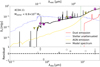 |
Fig. B.1. SED fitting model and photometric data. In the upper panel, we show the fitted SED model spectrum from X-CIGALE with a black curve. In addition, dust and unattenuated stellar and AGN emissions are shown in red, blue dotted, and yellow curves, respectively. The input observed photometry flux densities are marked in dark magenta boxes and olive triangles (upper limits). The X-ray data are not shown as they do not constrain the stellar component. The green vertical dashed line is the position of rest frame 1.6 μm from which the unattenuated stellar flux is adopted for Mstellar estimation. In the lower panel, we present the relative residuals, |
Appendix C: Notes on the master spectra fitting
C.1. Fitting procedure implementation
During the process of implementing the MCMC fitting, we notice that the numerical approximation of the Voigt profile by Tepper-García (2006, 2007) may not behave well at the center, that is, the Voigt function (Eq. A.6) will return a double-peak feature when x → 0. Hence, we manually set
(T. Tepper-García, priv. comm.). We also test the possibility using a more sophisticated function, the Faddeeva function, to approximate the Voigt function following Bolmer et al. (2019). It, however, does not perform well to produce the expected result, probably because the resolution of MUSE does not allow such a delicate function to work. Hence, we keep the Tepper-García (2006, 2007) approximation (Eq. A.6), which has proven to be successful on MUSE data (Kolwa et al. 2019).
C.2. Lyα fitting notes
In this appendix, we discuss the details and uncertainties run into during the Lyα fitting. For the continuum with relatively low flux underneath the Lyα, we decide to fit it using a first-order polynomial function and let the slope and intercept as free parameters during the further Gaussian+Voigt fitting. We describe how sensitive the H I absorption fitting results are with respect to different continuum fitting strategies in Appendix D.
As shown in Fig. 3, the Lyα line is asymmetric and highly absorbed. It can be fitted with the systemic redshift determined from He II (Sect. 4.2). To fit this complicated line with Gaussian+Voigt profile with many free parameters, it is challenging without any prior-knowledge (unlike Kolwa et al. 2019, which has a previous high spectral resolution UV spectrum analysis as guidance). Since all absorbers identified here are located at the blue wing (one near the v = 0 km s−1) of the Lyα line, we first use only the red wing of Lyα to constrain the unabsorbed, intrinsic emission. Then, we add Voigt profiles to model the H I absorbers following the procedure described in 3.2. However, it is still impossible to fit all eight absorbers simultaneously without the initial values of NH and b confined to an accurate range. Hence, we first start with fitting the first four absorbers with the data input just covering their spectral range and add more absorbers when satisfied with the previous step. There are at least eight H I absorbers. We decide not to include further ones due to the low S/N and their large velocity shifts indicating them being outside the galactic potential well. As discussed in Sect. 3.2, the primary fit is performed using the least-squares method and is then changed to MCMC later using the results from least-squares as initial inputs for accurate results and uncertainties. The boundary conditions applied to the Lyα fitting are shown in Table C.1. We follow Kolwa et al. (2019) to constrain the H I column density to be within 1013 − 1020 cm−2.
Boundary constrains for the parameters of Lyα fitting using MCMC method.
The Lyα blueshifted Gaussian component is at ∼ − 102 km s−1, which is the boundary manually set. If no constraints are applied in the final fit, both Gaussian emission components would be at ∼0 km s−1, which would lead to an underestimation of the flux on the blue wing. This is probably due to the red wing being un-absorbed to which the algorithm gives high weight. We limit the line center (< − 100 km s−1) of the broad component to be blueshifted to account for the flux excess between absorbers #7 and #8 (Fig. 3).
We note that the Doppler parameters of absorbers #4 and #5 have large values exceeding 200 km s−1, which may indicate that we are observing two or more spectrally unresolved absorbers with similar velocity shifts. This may be a the similar situation as observed for MRC 0200+015 using low- and high-resolution spectrographs (van Ojik et al. 1997; Jarvis et al. 2003). We test this by including two secondary absorbers (#4a and #5a) close to absorbers #4 and #5 when performing the fitting. There is no significant improvement and values of the fitted parameters of absorbers #4, #4a, #5, and #5a are not well constrained, and we therefore do not further regard this option. This issue may be revisited in the future using higher spectral resolution data.
C.3. C IV and He II fitting notes
We describe several strategies used in Sect. 4.2 to fit the C IV and He II lines, which have low S/N. In this appendix, we present details and reasons for the adjustment and discuss some uncertainties faced in running the fitting. In particular, we adjust the fitting procedure described in Sect. 3.2 in the following eight aspects.
MCMC fitting constrains of C IV + He II and N V.
First, we fit C IV and He II simultaneously. Because C IV, which is also a doublet, suffers from absorption and may contain several kinematic emission components, it is better to fix the line center of its intrinsic emission with the redshift determined by the He II.
Second, we fixed the continuum level underneath these two lines, which is determined beforehand with emissions lines masked. Third, we excluded the wavelength ranges from the fitting where the contribution of skylines is significant (marked as yellow shaded regions in Fig. 4).
Fourth, we removed the potentially blueshifted broad component of the C IV intrinsic emission, which is probably heavily absorbed. This could be the same emission component we included in the Lyα fitting (Sect. 4.1).
Fifth, to alleviate the removal of this blueshifted component, we adopted a Lorentzian profile instead of a single Gaussian to account for the broad wings of both C IV and He II. The Lorentzian may not be the best physical description of the underlying emission profile, but it is the best solution given the limited S/N to allow for absorption fits in the C IV blue side. Sixth, since the C IV is very broad (Fig. 4), we included an additional set of Gaussian to account for the extreme (> 1000 km s−1) blueshifted component.
Seventh, to account for the absorption, we included four C IV absorbers that we assumed to be the same ones causing the Lyα absorption (Sect. 4.1). The reason we only included four absorbers instead of all eight is that the positions of absorber #5 and beyond are in the low flux and S/N part of the C IV lines, which also suffers from skyline contamination and cannot be robustly fitted. We notice that we allow the redshift of the absorbers to be free within a limited range (Δz = 0.006 for absorber #1, Δz = 0.004 for absorber #4) following Kolwa et al. (2019) who argues that fixing the redshift of absorption caused by different species is un-physical given their different ionization energies.
Finally, we fixed the Doppler parameters and redshifts of absorbers #2 and #3 to the values derived from H I absorbers #2 and #3. We also set the ranges of the column densities to 1011.5 − 1012 cm−1 and 1012 − 1014 cm−1 for absorbers #2 and #3, respectively. These are implemented due to the large overlapping of these two absorbers (with others), which leads to a failure of fitting without further constrains.
The initial guess for the redshift (He II line center), 4.514, is adopted from Kopylov et al. (2006) and is used only in the least-squares fitting. After the redshift constrained to a relatively satisfied range, we allow it to vary within ±2 Å during the MCMC fitting. The velocity shift of the blueshifted C IV component is left relatively free with a broad range, −3000 ∼ −500 km s−1. The results from ∼ − 1500 km s−1 to ∼ − 900 km s−1 will all give us satisfied overall fit. This is also indicated by the distribution of LC IV,2, line center of the blueshifted component, seen in Fig. E.4, which has a long tail toward the lower values. Based on this, we argue in Sect. 4.3 that the blueshifted component of C IV and N V likely result from the same gaseous cloud. The boundaries of the Doppler parameters, b, and column density, NC IV, are set to 40 − 400 km s−1 and 1013 − 1016 cm−2, respectively (stricter settings for absorber #2 and #3 as mentioned above) following Kolwa et al. (2019). Table C.2 summarizes the constraints used in the C IV and He II fitting. The rules for line center, line width and line flux of the doublet are presented as well as the constraints of the absorption parameters of the doublet.
The major result we interested in from the He II fitting is the systemic redshift. We test the possibility of using a double Gaussian to fit the He II. The result is similar (4.5079 ± 0.0001 and 4.5077 ± 0.0001) to the Lorentzian fit and shows that the algorithm will fit both of the line centered at Δv ∼ 0 km s−1. This further indicates that the S/N of the line is not enough to fit the two Gaussian.
We test the possibilities of using (i) only absorbers #1 and #4 or (ii) absorbers #1, #3, and #4 to fit the CIV, which is under the assumption that absorbers #2 and/or #3 have low metallicity. Both settings (i) and (ii) have similar results for absorbers #1 and #4. Hence, we include all four absorbers and avoid the strong assumption.
C.4. N V fitting notes
The position of the N V is at the broad wing of Lyα. The flux excess we see on Fig. 3 above the fitted Lyα model at around 5000 km s−1 is due to the contribution of the blueshifted N V component. In addition, the low flux and highly absorbed systemic emission make N V a non-obvious detection.
As described in Sect. 4.3, we fix the best-fit Lyα model from Sect. 4.1 and use a constant continuum when fitting the N V. The reasons we do not apply the same continuum level for Lyα and N V lines are: (i) we test in Appendix D that using a continuum determined from the red wing and free first-order polynomial have similar results for the H I fitting (Appendix D); (ii) the first-order polynomial will slightly overestimate the continuum flux of Lyα red wing whose influence is probably negligible for Lyα, which is a broad line with high flux. For N V, however, which is at longer wavelength than Lyα and has extremely low S/N, the continuum overestimation will affect the fit more. This is indeed the case when the first-order polynomial continuum is applied during the N V fitting, which results in poor constraints.
As we see in Fig. E.6, the line center of the blueshifted component, LN V,b, and Doppler parameter, b1, are not fully constrained. For LN V,2, we set the range −1600 ∼ −500 km s−1 according to C IV blueshifted component. The reason it hits the lower boundary is due to the influence of Lyα red wing. As mentioned in Appendix E.2, the velocity shift down to −1500 km s−1 will still give satisfying results for the C IV fit. The main parameter in this fit, NN V, does not change much if we vary the given boundary of the line center of the blueshifted component. Besides, we test to leave it relatively free and end up with poor fit quality (unphysical result). Therefore, we manually set this lower boundary, which results in a satisfying fit given the low S/N. More importantly, this velocity shift shows the consistence between N V and CIV, which agrees with the hypothesis. For b1, which hits the upper boundary, we tested fixing it to the value obtained from C IV absorber #1, which results in a poor fit quality as well. This could probably be due to (i) the low S/N of the N V; (ii) the influence of the unresolved H I redshifted absorber(s); (iii) the imperfect sky line subtraction. Hence, we present this fit and remind the readers to be cautious about the NN V, which should be considered as a lower limit given the well-known b − N degeneracy (Silva et al. 2018a).
Appendix D: Lyα continuum sensitivity test
The Lyα emission of quasars and galaxies at high redshift are highly absorbed by the intervening hydrogen clouds located between observer and source. This so-called Lyα forest (e.g., Adelberger et al. 2003) heavily affects the blue wing of Lyα making it difficult for continuum fitting. For our MUSE observation, the spectral resolution is too low to resolve the narrow intervening absorbers, but we can clearly identify a change between the continuum of the blue and red side of the Lyα, namely the continuum flux is lower in the blue than the red. Several potential methods can be used to fit this continuum. Hence, we run a test to see how significant the change that different continuum fitting strategies may cause the absorption fitting. We use five different methods, which are described below.
In the first method, the continuum is fitted using a first-order polynomial prior to the Gaussian+Voigt fitting and fixed during the following fitting. The wavelength range used in this method for the continuum is 6405 − 6986 Å (−13 000 ∼ 13 000 km s−1) with the emission region masked.
For the second method, the continuum is fitted using a first-order polynomial together with the Gaussian+Voigt fitting. The values of slope and intercept from method 1 are used as initials.
In the third method, the continuum is fitted using a zero order polynomial of the red wing and fixed during the Gaussian+Voigt fitting. The wavelength range used in this method for the continuum is 6880 − 6986 Å (8 258 ∼ 13 000 km s−1). We chose the wavelength range to be at extremely red wing of the Lyα to avoid the contamination of the N V (Sect. 4.3 and Appendix C.4).
For the fourth method, the continuum is fitted using a zero order polynomial of the blue wing and fixed during the Gaussian+Voigt fitting. The wavelength range used in this method for the continuum is 6405 − 6600 Å (−13 000 ∼ −4 300 km s−1).
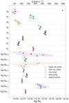 |
Fig. D.1. MCMC fitted Voigt parameters, NH and b, of the eight H I absorbers from five continuum fitting methods. The subscripts 1−8 represent the indices of the absorbers. The colors represent different parameters (the same color is used for the NH and b of the same absorber), while the mark styles indicate different continuum fitting methods. |
As for the fifth method, the continuum is fitted using a step function. The wavelength of the step is fitted together with the Gaussian+Voigt fitting. The left (right) value is set to the one from blue (red) wing zero order polynomial result and fixed during the fit.
The result is shown in Fig. D.1 in which the fitted Voigt parameters using MCMC method, NH I and b, of the eight absorbers from different continuum fitting strategies are presented. It is intuitive to identify that most of the fitted values from different continuum methods are consistent, though some have relatively large scatters (e.g., absorbers #6−8), which is understandable given that these absorbers are located at the low S/N tail. Therefore, we decided that the continuum fitting method has a minor effect on the absorption parameters, which is our primary focus in this work. By checking the corner plots produced from these five methods, we find that fitting the first-order polynomial continuum together with the Gaussian+Voigt model (method 2) constrains the probability distribution of the absorption parameters (z, b, and NH I) best. Hence, we use the method 2 when doing the Lyα fit. Using a first-order polynomial to fit the continuum is a commonly used method (e.g., Kolwa et al. 2019), and giving freedom to the slope and intercept will constrain better the line features.
As for the spatially resolved Lyα analysis, we first fit the continuum level of the spectra in each spatial bin with emission part masked. We then keep the continuum fixed to this level when running the Gaussian+Voigt fitting. Because, for consistence, we use the same model for fitting each of the 64 spectrum (see Sect. 3.3) and some spectra have lower S/N ratios, which may affect the fitting if we add more free parameters (for the continuum).
Appendix E: Auxiliary materials of MCMC fitting
 |
Fig. E.1. Acceptance fraction of each walker used in the Lyα MCMC fitting. |
In this appendix, we present some side products of the MCMC fitting, which can be used as auxiliary materials to better understand the fitting quality, namely the corner plot and acceptance fraction plot. The corner plot is a tracer for the probability distributions of the fitted parameters and correlation between each parameters; in other words, we can identify the degeneracy between fitted parameters from the corner plot. The acceptance fraction plot is used to check the acceptance fraction of each walker used in MCMC (see Foreman-Mackey et al. 2013, for details). This can be used as an easy check of the performance of the MCMC run. Although some details are not clear, the acceptance fraction lies in 0.2−0.5 is thought to be an indication of a successful run (Foreman-Mackey et al. 2013).
E.1. Lyα
The acceptance fraction and corner plot of MCMC fitting of master Lyα are shown in Fig. E.1 and E.2, respectively. In Fig. E.1, we can see that a number of walkers are rejected with a mean acceptance fraction of 0.11. This is due to the larger number (32) of free parameters used in the Lyα fitting. In Fig. E.2, we identify several banana shapes of the correlation distribution (e.g., between bi and NHi). This is a well-known degeneracy in the Voigt fitting (e.g., Silva et al. 2018a) that a combination of larger N value and smaller b value can the overall similar result with a combination of smaller b and larger N.
E.2. C IV and He II
The acceptance fraction and corner plot of MCMC fitting of master C IV He II are shown in Fig. E.3 and E.4, respectively. In Fig. E.3, we can see that the acceptance fraction of all of the walkers are in the range of 0.2 − 0.5 with a mean of 0.26. This is evidence indicating the success of the fitting. In Fig. E.4, we see that the probability distributions of NC IV2 and NC IV3 have tentative peak and un-defined tail to the lower value. This is more severe for absorber #2 given that the lower boundary we apply (1011.5 cm−2) is extremely low. Based on the above, we decide to treat the column density of absorber #2 and #3 as upper limit.
 |
Fig. E.2. Corner plot derived from the MCMC fitting of the Lyα line (see Sect. 4.1). In this figure we only show the correlation between the absorption parameters, namely zi, bi, and NC IVi, which are the fitted redshifts, Doppler parameters (in units of km s−1), and column densities (logarithmic) of the eight H I absorbers. The black dotted lines in each of the histograms represent 15.8 and 84.2 percentiles, which correspond to the reported uncertainty ranges. The blue solid lines mark the median and reported fit values, respectively. |
E.3. N V
The acceptance fraction and corner plot of the MCMC fitting of the master N V are shown in Fig. E.5 and E.6, respectively. In Fig. E.5, we can see that all walkers are in the range of 0.2−0.5 with a mean of 0.41, which indicates the MCMC fitting of N V is successful. We discuss the uncompleted sampled distribution of LN V,b and b1 in Appendix C.4.
E.4. O III]
The acceptance fraction and corner plot of the MCMC fitting of master O III] are shown in Fig. E.7 and E.8, respectively. We perform the MCMC fitting for this two-free-parameter model to be consistent with other fittings. In Fig. E.7, we can see that all walkers are above 0.5 with a mean of 0.72, which indicates that the model is probably over-fitted.
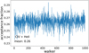 |
Fig. E.3. Acceptance fraction of each walker used in the C IV and He II MCMC fitting. |
 |
Fig. E.4. Corner plot derived from the MCMC fitting of the C IV and He II (see Sect. 4.2). In this figure we show the correlation between the free parameters in the C IV+He II fit. The λHe II and λC IV,2 are the line centers of the He II and blueshifted C IV (for the 1548 Å line) emissions in Å, respectively. The FHe II, FC IV,1, and FC IV,2 are the integrated line fluxes of He II, systemic C IV, and blueshifted C IV (only for the 1548 Å line) emissions in 10−20 erg s−1 cm−2 Å−1, respectively. The FWHMHe II, FWHMC IV, and σC IV,2 are the line widths of He II, systemic C IV, and blueshifted C IV (for the 1548 Å line) emissions in Å. zi, bi, and NC IVi, which are the fitted redshifts, Doppler parameters (in units of km s−1), and column densities (logarithmic) of the four absorbers. The black dotted lines in each of the histograms represent 15.8 and 84.2 percentiles, which correspond to the reported uncertainty ranges. The blue solid lines mark the median and reported fit values, respectively. |
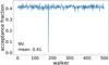 |
Fig. E.5. Acceptance fraction of each walker used in the N V MCMC fitting. |
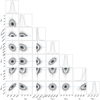 |
Fig. E.6. Corner plot derived from the MCMC fitting of the N V (Sect. 4.2). In this figure we show the integrated line flux (FN V in 10−20 erg s−1 cm−2 Å−1) and the Gaussian line width (σN V, in Å) of the systemic N V emission; the line center (LN V,b in Å), integrated line flux (FN V,b), and Gaussian line width (σN V,b) of the blueshifted N V component (for the 1238 Å line); and the Doppler parameter (b1) and column density (NN V,1) of absorber #1. The black dotted lines in each of the histograms represent 15.8 and 84.2 percentiles, which correspond to the reported uncertainty ranges. The blue solid lines mark the median and reported fit values, respectively. |
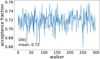 |
Fig. E.7. Acceptance fraction of each walker used in O III] MCMC fitting. |
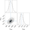 |
Fig. E.8. Corner plot derived from the MCMC fitting of the O III] (Sect. 4.4). The FO III and σO III are the integrated line flux and line width of the 1660.81 Å doublet line, respectively. The black dotted lines in each of the histograms represent 15.8 and 84.2 percentiles, which correspond to the reported uncertainty range. The blue solid lines mark the median and reported fit values, respectively. |
Appendix F: Individual Lyα spectra fitting
In this appendix, we present the Lyα fitting results from each individual bins described in Sects. 3.3 and 5.1 in Fig. F.2 to F.5. The spatial region (bin) from which each of the presented spectrum is extracted is shown in Fig. F.1. The spatial bins are numbered (and color-coded) and are the same as those marked in Figs. F.2 to F.5 in order to trace their spatial location. The details of the tessellation is described in Sect. 3.3.
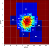 |
Fig. F.1. Spatial binning results from Sect. 3.3. The colors represents different bins. The bin numbers correspond to the numbers marked in Figs. F.2–F.5. The black or white colors of the bin number are given to better distinguish it from the color of the bin. |
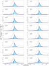 |
Fig. F.2. Spectra extracted from the 64 spatial bins (see Sect. 3.3) and Gaussian+Voigt fitting results. In each panel, the thick dark magenta line indicates the best fit model. The dot-dash red line and dashed blue line denote the narrow and broad emission components, respectively. The dotted olive lines are the summation of the two emissions. The |

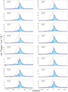 |
Fig. F.3. Figure F.2 continued. |
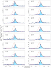 |
Fig. F.4. Figure F.3 continued. |
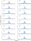 |
Fig. F.5. Figure F.4 continued. |
Appendix G: C IV spatial mapping
In this appendix we present the parameters derived from the C IV spatial fitting (see Sect. 5.2). The fittings are done for He II and C IV simultaneously with the similar procedure described in Sects. 3.2 and 5.2. The emission results for both He II and C IV from NE and SW are presented in Table G.1. In Table G.2, we show the absorption fitting results of the 4 C IV absorbers from these two regions. For comparison, we also show the emission and absorption fitting results of the Lyα lines from these two regions in the corresponding tables. Due to the low S/N of the two C IV spectra and in order to avoid overfitting, we fix the z and b of the absorbers in the fit and use the derived column densities as upper limit. The exception is the column density of absorber #1 of the NE spectrum, which has a well distributed probability extracted from the corner plot. The distribution is presented in Fig. G.1 in blue with a well defined peak. We also show the distribution of the same absorber from the SW spectrum for comparison in this figure in orange. We note that the z and b for the absorbers in both of the NE and SW C IV spectra are fixed to the corresponding values derived from master Lyα during the fitting. It will cause unsuccessful fitting if we use the fitted values from NE and SW Lyα to fix the corresponding C IV fits. We argue that the adopted choice is reasonable because (i) large parts of the NE and SW regions are covered by the master aperture; (ii) the master Lyα has high S/N.
Best fitted emission results of the 1D aperture-extracted spectrum from the NE and SW regions using the MCMC method.
Best absorption fitting results of the 1D aperture-extracted spectrum from the NE and SW regions using the MCMC method.
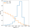 |
Fig. G.1. Probability distributions of the C IV absorber #1 column density extracted from the corner plots. The blue and orange histograms represent the results of the NE and SW spectra, respectively. |
All Tables
Best fitted emission results of the 1D aperture-extracted spectrum using the MCMC method.
Best absorption fitting results of the 1D aperture-extracted spectrum using the MCMC method.
Best fitted emission results of the 1D aperture-extracted spectrum from the NE and SW regions using the MCMC method.
Best absorption fitting results of the 1D aperture-extracted spectrum from the NE and SW regions using the MCMC method.
All Figures
|
Fig. 1. Lyα narrowband surface brightness (SB) image of 4C04.11 derived from the data cube using 6704 − 6710 Å in the observed frame. The blue contour indicates the He II emission region. The contour is calculated from the pseudo-narrowband image of He II using 9028 − 9044 Å in the observed frame with the level of 3σHe II and 2 × 3σHe II, where σHe II is the standard deviation derived from a source-less region of the He II pseudo-narrowband image. The white contour traces the position of the radio jet observed by MERLIN (Multi-Element-Radio-Link-Interferometer-Network; Parijskij et al. 2013, 2014) with the level of 0.45 × (−1, 1, 2, 4, 16, 32, 48) mJy beam−1 following Parijskij et al. (2014). The overlaid red circle with a 1 arcsec radius marks the aperture over which the master spectrum is extracted. The green dashed box shows the FOV of individual panels in Figs. 7 and 8, which is the region we focus on in the spatial mapping in Sect. 5. |
| In the text | |
|
Fig. 2. Rest frame UV spectra of 4C04.11. Upper panel: full MUSE spectrum extracted from the central 1 arcsec aperture region. We refer to this spectrum as the master spectrum. The detected UV lines (Lyα, C IV, He II, and O III]) are marked with red dashed lines. We also mark the N V, which has a low S/N, overlaps with the broad Lyα wing, and is not obvious in this full spectrum (see Sect. 4.3). We use the black dotted line to indicate the position of the undetected Si IV. Lower panel: same plot as the upper panel but zoomed in to show the continuum. We note that the skyline residuals are seen as regions with higher noise. The horizontal black dashed line marks the zero flux level. |
| In the text | |
|
Fig. 3. Lyα fitting result and model sensitivity check. Upper panel: best fitting result of the master Lyα line using the MCMC method. The dark magenta line represents the best fit, while the dotted olive line traces the overall Gaussian emission. The systemic emission is shown in a red dotted-dashed line, and the blueshifted emission is marked by a blue dashed line. The positions of all eight absorbers are shown in this panel with black vertical bars. The |
| In the text | |
|
Fig. 4. Best fit of the C IV and He II lines from the master spectrum using the MCMC method. We use the dark magenta line to trace the best fit of these two lines. For the intrinsic C IV and He II, the yellow dotted line is used. We mark the systemic emissions of the C IV doublet in dotted green and dashed red lines and blueshifted emissions in dotted and dot-dash blue lines. The |
| In the text | |
|
Fig. 5. N V best-fit model from MCMC method. The dark magenta line shows the best N V fit combined with the Lyα from Sect. 4.1. The black dashed line marks all combined emissions without absorption. The systemic emissions are marked in dotted green, and dashed red curves show the doublet. The zero velocities of the systemic emissions for the doublet components are derived from the He II result. The blueshifted components are shown in dotted and dot-dash blue lines for the doublet. The solid olive line shows the Lyα model, which is fixed in the N V fit. The short green (red) vertical bars with numbers show the positions of the absorbers on top of the N Vλ1239 (N Vλ1243) line. The dashed line style and lighter color are used to indicate that N V absorber #1 is marginally constrained (see text). The |
| In the text | |
|
Fig. 6. O III] best-fit model using the MCMC method. The dark magenta line shows the best O III] fit combined with the He II from Sect. 4.2. The emissions of the O III] doublet are shown in dotted green and dashed red curves. The line centers of the systemic emissions expected for the doublet components from the He II implied redshift are shown in vertical dotted green and red lines. The solid olive line shows the He II model that is fixed in the O III] fit. The |
| In the text | |
|
Fig. 7. Spatial mapping results of Lyα emission. The contours are the same in all panels, with the green showing the position of the radio source (see the Fig. 1 caption for details; Parijskij et al. 2013, 2014) and black tracing the Lyα surface brightness resulting from spatial fitting (the levels are given arbitrarily). All these maps are constructed based on the fitting results, i.e., not directly from the data. (a) Intrinsic surface brightness map of Lyα emission. (b) W80 map of Lyα emission (nonparametric measurement of the line width; see text). (c) v50 map of the fitted Lyα emission profile (nonparametric measurement of the line-of-sight velocity; see text). |
| In the text | |
|
Fig. 8. Column density and velocity shift maps of H I absorber #1 (panels a and b) and #2 (panels c and d). The black contours are the same as in Fig. 7. The zero points for the velocity shift maps are chosen individually to be the Δv of each absorber as derived from the master spectrum fitting reported in Table 2. The maps therefore show the velocity shifts relative to the redshift of the respective absorber. |
| In the text | |
|
Fig. 9. C IV broadband image clasped between 8400 − 8600 Å in the observed frame. The white contour traces the radio jet, while the red circle marks the position where the spectrum analyzed in Sect. 4 is extracted (see the caption of Fig. 1). The dark blue and magenta regions show the apertures from which the spectra used to studied the spatial features of C IV are extracted. The spectrum from the dark blue (magenta) region is marked as NE (SW). |
| In the text | |
|
Fig. 10. Spectra and fit of Lyα (top row) and C IV (middle row) and noise spectra of C IV (lower row) extracted from the dark blue (NE) and magenta (SW) regions shown in Fig. 9. The positions of H I absorber #1 are marked with black bars in the top row. The velocity shift is relative to the systemic redshift, z = 4.5077, fitted from He II (Sect. 4.2). The line styles used to show the fitting results are the same ones as that of the master Lyα (Fig. 3) and C IV (Fig. 4). We note that except for C IV absorber #1 detected in the NE region, the positions for the other C IV absorbers are marked in dashed bars, with lighter colors indicating that they are only marginally constrained (see text), which is consistent with the “master C IV” presentation (Fig. 4). The intrinsic C IV emission is also shown in orange dotted lines for the two spectra in the middle row. The panels in the bottom row show the standard deviations (noise) of the C IV spectra derived from the variance extension of the data cube, which are used as fitting weights. They are shown in the same units as the data spectra and can be used to show the quality of the spectra and trace the positions of skylines. |
| In the text | |
|
Fig. 11. Comparison between the Lyα, He II, and [O II] rest-frame spectra. The Lyα and He II presented here are the same ones analyzed in Sects. 4.1 and 4.2 in velocity scale. We subtract the continuum from the He II here to better present the low flux region of the emission. The black lines are the same ones as shown in Fig. 4 for the blueshifted He II models, with the dashed, dotted, and dash-dotted lines indicating the line flux of 0.2, 0.3, and 0.4 of the total fitted flux of the blueshifted C IV. The [O II] is taken from SINFONI (Nesvadba et al. 2017a). In each panel, the black dashed lines indicate the zero velocity. In the last two panels, the dashed vertical teal blue lines show the velocity shift of the C IV blueshifted component. For Lyα and He II, the best fit models from this work are shown. We also mark the fitted line centers of the [O II] narrow doublet from Nesvadba et al. (2017a) in pink dotted lines and the broad component line center in a pink dash-dot line. |
| In the text | |
|
Fig. 12. Schematic view of the proposed outflowing shell model in Sect. 7.1. The large dark green annulus represents the outflowing gaseous shell that could be the absorbing cloud of absorber #1. The blue and orange regions mark the southern (approaching) and northern (receding) jet hotspot interacting with the previous ejected shell, respectively. We note that the morphology of the gaseous shell is not necessarily in a circular shell as shown here, and we do not have information for the shell at the backside of the AGN. The red lines in the annulus center indicate the region of the AGN ionization cone that could have a wider opening angle than the jet beam (see text). The column density gradient we observed in Sect. 5.1 in the S-N (SW-NE, due to the orientation on the sky plane, which is not shown here) direction could simply be explained by the different lengths of the observer line of sight intersecting with the gaseous shell at different spatial locations (see text). This process is shown with the length of white arrows intersecting with the dark green annulus in the figure. For the column density decreasing after passing the midplane, which cannot be explained by the geometry setting, the southern jet (blue region) interaction with the ejected gaseous shell could cause the decreasing of column density through instabilities and/or partially ionizing the gas. Though the rough projection size of the jet is shown, we note that other parts of this sketch are not to scale. |
| In the text | |
|
Fig. B.1. SED fitting model and photometric data. In the upper panel, we show the fitted SED model spectrum from X-CIGALE with a black curve. In addition, dust and unattenuated stellar and AGN emissions are shown in red, blue dotted, and yellow curves, respectively. The input observed photometry flux densities are marked in dark magenta boxes and olive triangles (upper limits). The X-ray data are not shown as they do not constrain the stellar component. The green vertical dashed line is the position of rest frame 1.6 μm from which the unattenuated stellar flux is adopted for Mstellar estimation. In the lower panel, we present the relative residuals, |
| In the text | |
|
Fig. D.1. MCMC fitted Voigt parameters, NH and b, of the eight H I absorbers from five continuum fitting methods. The subscripts 1−8 represent the indices of the absorbers. The colors represent different parameters (the same color is used for the NH and b of the same absorber), while the mark styles indicate different continuum fitting methods. |
| In the text | |
|
Fig. E.1. Acceptance fraction of each walker used in the Lyα MCMC fitting. |
| In the text | |
|
Fig. E.2. Corner plot derived from the MCMC fitting of the Lyα line (see Sect. 4.1). In this figure we only show the correlation between the absorption parameters, namely zi, bi, and NC IVi, which are the fitted redshifts, Doppler parameters (in units of km s−1), and column densities (logarithmic) of the eight H I absorbers. The black dotted lines in each of the histograms represent 15.8 and 84.2 percentiles, which correspond to the reported uncertainty ranges. The blue solid lines mark the median and reported fit values, respectively. |
| In the text | |
|
Fig. E.3. Acceptance fraction of each walker used in the C IV and He II MCMC fitting. |
| In the text | |
|
Fig. E.4. Corner plot derived from the MCMC fitting of the C IV and He II (see Sect. 4.2). In this figure we show the correlation between the free parameters in the C IV+He II fit. The λHe II and λC IV,2 are the line centers of the He II and blueshifted C IV (for the 1548 Å line) emissions in Å, respectively. The FHe II, FC IV,1, and FC IV,2 are the integrated line fluxes of He II, systemic C IV, and blueshifted C IV (only for the 1548 Å line) emissions in 10−20 erg s−1 cm−2 Å−1, respectively. The FWHMHe II, FWHMC IV, and σC IV,2 are the line widths of He II, systemic C IV, and blueshifted C IV (for the 1548 Å line) emissions in Å. zi, bi, and NC IVi, which are the fitted redshifts, Doppler parameters (in units of km s−1), and column densities (logarithmic) of the four absorbers. The black dotted lines in each of the histograms represent 15.8 and 84.2 percentiles, which correspond to the reported uncertainty ranges. The blue solid lines mark the median and reported fit values, respectively. |
| In the text | |
|
Fig. E.5. Acceptance fraction of each walker used in the N V MCMC fitting. |
| In the text | |
|
Fig. E.6. Corner plot derived from the MCMC fitting of the N V (Sect. 4.2). In this figure we show the integrated line flux (FN V in 10−20 erg s−1 cm−2 Å−1) and the Gaussian line width (σN V, in Å) of the systemic N V emission; the line center (LN V,b in Å), integrated line flux (FN V,b), and Gaussian line width (σN V,b) of the blueshifted N V component (for the 1238 Å line); and the Doppler parameter (b1) and column density (NN V,1) of absorber #1. The black dotted lines in each of the histograms represent 15.8 and 84.2 percentiles, which correspond to the reported uncertainty ranges. The blue solid lines mark the median and reported fit values, respectively. |
| In the text | |
|
Fig. E.7. Acceptance fraction of each walker used in O III] MCMC fitting. |
| In the text | |
|
Fig. E.8. Corner plot derived from the MCMC fitting of the O III] (Sect. 4.4). The FO III and σO III are the integrated line flux and line width of the 1660.81 Å doublet line, respectively. The black dotted lines in each of the histograms represent 15.8 and 84.2 percentiles, which correspond to the reported uncertainty range. The blue solid lines mark the median and reported fit values, respectively. |
| In the text | |
|
Fig. F.1. Spatial binning results from Sect. 3.3. The colors represents different bins. The bin numbers correspond to the numbers marked in Figs. F.2–F.5. The black or white colors of the bin number are given to better distinguish it from the color of the bin. |
| In the text | |
|
Fig. F.2. Spectra extracted from the 64 spatial bins (see Sect. 3.3) and Gaussian+Voigt fitting results. In each panel, the thick dark magenta line indicates the best fit model. The dot-dash red line and dashed blue line denote the narrow and broad emission components, respectively. The dotted olive lines are the summation of the two emissions. The |
| In the text | |
|
Fig. F.3. Figure F.2 continued. |
| In the text | |
|
Fig. F.4. Figure F.3 continued. |
| In the text | |
|
Fig. F.5. Figure F.4 continued. |
| In the text | |
|
Fig. G.1. Probability distributions of the C IV absorber #1 column density extracted from the corner plots. The blue and orange histograms represent the results of the NE and SW spectra, respectively. |
| In the text | |
Current usage metrics show cumulative count of Article Views (full-text article views including HTML views, PDF and ePub downloads, according to the available data) and Abstracts Views on Vision4Press platform.
Data correspond to usage on the plateform after 2015. The current usage metrics is available 48-96 hours after online publication and is updated daily on week days.
Initial download of the metrics may take a while.