| Issue |
A&A
Volume 680, December 2023
|
|
|---|---|---|
| Article Number | A70 | |
| Number of page(s) | 44 | |
| Section | Extragalactic astronomy | |
| DOI | https://doi.org/10.1051/0004-6361/202346415 | |
| Published online | 12 December 2023 | |
3D tomography of the giant Lyα nebulae of z ≈ 3–5 radio-loud AGN
1
Astronomisches Rechen-Institut, Zentrum für Astronomie der Universität Heidelberg, Mönchhofstr. 12-14, 69120 Heidelberg, Germany
e-mail: This email address is being protected from spambots. You need JavaScript enabled to view it.
; This email address is being protected from spambots. You need JavaScript enabled to view it.
2
European Southern Observatory, Karl-Schwarzchild-Str. 2, 85748 Garching, Germany
3
Cosmic Dawn Center, Copenhagen, Denmark
4
DTU Space, Technical University of Denmark, Elektronvej 327, 2800 Lyngby, Denmark
5
Centre for Extragalactic Astronomy, Department of Physics, Durham University, South Road, Durham DH1 3LE, UK
6
Centro de Astrobiología, CSIC-INTA, Ctra. de Torrejón a Ajalvir, km 4, 28850 Torrejón de Ardoz, Madrid, Spain
7
Univ. Lyon, Univ. Lyon1, ENS de Lyon, CNRS, Centre de Recherche Astrophysique de Lyon UMR5574, 69230 Saint-Genis-Laval, France
8
International Centre for Radio Astronomy Research, Curtin University, 1 Turner Avenue, Bentley, WA 6102, Australia
9
Max-Planck-Institut fur Astrophysik, Karl-Schwarzschild-Str 1, 85748 Garching bei München, Germany
10
Instituto de Astrofísica e Ciências do Espaço, Universidade do Porto, CAUP, Rua das Estrelas, 4150-762 Porto, Portugal
11
Institute for Computational Astrophysics and Department of Astronomy & Physics, Saint Mary’s University, 923 Robie Street, Halifax, NS B3H 3C3, Canada
12
Physics Department, University of Johannesburg, 5 Kingsway Ave, Rossmore, Johannesburg 2092, South Africa
Received:
14
March
2023
Accepted:
26
September
2023
Abstract
Lyα emission nebulae are ubiquitous around high-redshift galaxies and are tracers of the gaseous environment on scales out to ≳100 pkpc (proper kiloparsec). High-redshift radio galaxies (HzRGs, type-2 radio-loud quasars) host large-scale nebulae observed in the ionised gas differ from those seen in other types of high-redshift quasars. In this work, we exploit MUSE observations of Lyα nebulae around eight HzRGs (2.92 < z < 4.51). All of the HzRGs have large-scale Lyα emission nebulae with seven of them extended over 100 pkpc at the observed surface brightness limit (∼2 − 20 × 10−19 erg s−1 cm−2 arcsec−2). Because the emission line profiles are significantly affected by neutral hydrogen absorbers across the entire nebulae extent, we performed an absorption correction to infer maps of the intrinsic Lyα surface brightness, central velocity, and velocity width, all at the last scattering surface of the observed Lyα photons. We find the following: (i) that the intrinsic surface brightness radial profiles of our sample can be described by an inner exponential profile and a power law in the low luminosity extended part; (ii) our HzRGs have a higher surface brightness and more asymmetric nebulae than both radio-loud and radio-quiet type-1 quasars; (iii) intrinsic nebula kinematics of four HzRGs show evidence of jet-driven outflows but we find no general trends for the whole sample; (iv) a relation between the maximum spatial extent of the Lyα nebula and the projected distance between the active galactic nuclei (AGN) and the centroids of the Lyα nebula; and (v) an alignment between radio jet position angles and the Lyα nebula morphology. All of these findings support a scenario in which the orientation of the AGN has an impact on the observed nebular morphologies and resonant scattering may affect the shape of the surface brightness profiles, nebular kinematics, and relations between the observed Lyα morphologies. Furthermore, we find evidence showing that the outskirts of the ionised gas nebulae may be ‘contaminated’ by Lyα photons from nearby emission halos and that the radio jet affects the morphology and kinematics of the nebulae. Overall, this work provides results that allow us to compare Lyα nebulae around various classes of quasars at and beyond cosmic noon (z ∼ 3).
Key words: galaxies: active / galaxies: evolution / galaxies: high-redshift / galaxies: halos / galaxies: jets
© The Authors 2023
 Open Access article, published by EDP Sciences, under the terms of the Creative Commons Attribution License (https://creativecommons.org/licenses/by/4.0), which permits unrestricted use, distribution, and reproduction in any medium, provided the original work is properly cited.
This article is published in open access under the Subscribe to Open model. This email address is being protected from spambots. You need JavaScript enabled to view it. to support open access publication.
1. Introduction
Being the most abundant element in the Universe, hydrogen (especially the cold gas, i.e. neutral hydrogen atoms and hydrogen molecules, H2) is the building block of the baryonic Universe. Studying H2 directly is difficult due to lack of prominent transition lines. It is often probed using low-J CO transitions as a proxy that unfortunately results in added uncertainties, for example in the conversion factor (e.g. Bolatto et al. 2013). In contrast, neutral atomic hydrogen can be easily ionised (EH0 = 13.6 eV) and cascade with line emissions being produced. The H I Lyαλ1216 (Lyα hereafter) line is the most prominent one among them. For high-redshift galaxies, it is a commonly targeted emission line that can easily be observed in the optical to near-infrared bands (e.g. Hu & McMahon 1996; Cowie & Hu 1998; Shimasaku et al. 2006; Dawson et al. 2007; Leclercq et al. 2017; Wisotzki et al. 2018; Umehata et al. 2019; Ono et al. 2021; Ouchi et al. 2020, and reference therein). Lyα emission can be detected on a range of spatial scales, for example at interstellar medium (ISM) to circumgalactic medium (CGM, Tumlinson et al. 2017) scales and even beyond the viral radius of the central object out to intergalactic medium (IGM) scales (e.g. Cantalupo et al. 2014; Cai et al. 2019; Ouchi et al. 2020). However, it is non-trivial to identify the origin of Lyα emission (e.g. due to the resonant nature of Lyα emission and various potential ionising sources acting at once), which is essential to understanding the physics of the emitting gas observed on different scales and around various types of objects (Dijkstra 2019; Ouchi et al. 2020). This is further complicated when active galactic nuclei (AGN) are present.
Active galaxies hosting AGN, especially the ones with quasar level activities (bolometric luminosity, Lbol ≳ 1045 erg s−1), at a high redshift are known to host Lyα nebulae on scales of a few 100 kpc (e.g. Heckman et al. 1991a; Basu-Zych & Scharf 2004; Weidinger et al. 2004, 2005; Dey et al. 2005; Prescott et al. 2015; Cantalupo et al. 2014; Arrigoni Battaia et al. 2016, 2019; Borisova et al. 2016; Cai et al. 2019). The central powerful AGN act as a main ionising mechanism for the surrounding gas, which is responsible for the detection of these extended Lyα nebulae (as predicted by theoretical works, e.g. Costa et al. 2022). In addition, the diffuse emission from galaxies near the AGN host can also contribute to the overall profile observed of the central target (e.g. Byrohl et al. 2021). In some of the giant nebulae, it is natural to find various mechanisms functioning at different scales and positions (e.g. Vernet et al. 2017). Therefore, despite leaving internal physics entangled, Lyα acts as a simpler tool for detecting a gaseous environment throughout cosmic time.
Before wide field integral field spectrographs (IFS) became available, narrow-band imaging and long slit spectroscopy provided effective methods to detect diffuse Lyα nebulae (e.g. Steidel et al. 2000; Francis et al. 2001; Matsuda et al. 2004; Saito et al. 2006; Yang et al. 2009, 2010; Cantalupo et al. 2012, 2014; Hennawi & Prochaska 2013; Prescott et al. 2015; Arrigoni Battaia et al. 2016). However, these observations have been limited by uncertainties in the systemic redshift measurements and limited spatial coverage, respectively. Integral field unit (IFU) observations – for example with the Multi-Unit Spectroscopic Explorer (MUSE/VLT) and Keck Cosmic Web Imager (KCWI/Keck) – allow us to measure the extent of the nebulae together with the information of their dynamics. Numerous works of Lyα nebulae around quasars report (tens of kiloparsecs to over 100 kpc) extended emission across a large range of redshifts (z ∼ 2 to z ∼ 6.3) and quasar types (e.g. radio-quiet and radio-loud type-1, radio-quiet type-2, and extremely red quasars, Christensen et al. 2006; Borisova et al. 2016; Arrigoni Battaia et al. 2019; Cai et al. 2019; Farina et al. 2019; den Brok et al. 2020; Fossati et al. 2021; Mackenzie et al. 2021; Lau et al. 2022; Vayner et al. 2023; Zhang et al. 2023). This diversity in nebula properties suggest a range of driving mechanisms, dependencies on orientation, and demonstrate that well-selected samples are needed. Despite the effort that has been made regarding this topic, a link between the aforementioned types and type-2 radio-loud quasars on a CGM scale is missing.
Among the high-redshift quasar population, high-redshift radio galaxies (HzRGs) are a unique sample despite being smaller in number (see Miley & De Breuck 2008, as a review). They host type-2 quasars and have powerful radio jets. They have been shown to reside in dense protocluster environments (Venemans et al. 2007; Wylezalek et al. 2013, 2014; Noirot et al. 2016, 2018), which may evolve to modern galaxy clusters. HzRGs were among the first sources where giant Lyα nebulae were discovered (∼1044 erg s−1, ≳100 kpc, e.g. Hippelein & Meisenheimer 1993; van Ojik et al. 1996, 1997; Reuland et al. 2003; Villar-Martín et al. 2006, 2007b) and observed with the previous generation of IFU instruments (e.g. Adam et al. 1997). The Lyα nebulae of HzRGs have been found to have two distinctive parts, namely the high surface brightness kinematically disturbed inner part and the quiescent low surface brightness extended outer nebula (e.g. Villar-Martín et al. 2002, 2003, 2007a). The spatial separation of these two parts seem to be consistent with the extent of the radio jets (e.g. Villar-Martín et al. 2003), suggesting that the jet plays a role in disturbing the inner part. Specifically, there is evidence that the Lyα nebulae around HzRGs are related to jet-driven outflows (Humphrey et al. 2006), while some of the quiescent gas may be related to infalling material (Humphrey et al. 2007). AGN photoionisation is likely the main mechanism of exciting these nebulae (e.g. Villar-Martín et al. 2002, 2003; Morais et al. 2017), but ionisation by fast shocks might also play a role (e.g. Bicknell et al. 2000; Morais et al. 2017). Polarisation measurements show that some of the Lyα emission in HzRGs is scattered (Humphrey et al. 2013). Despite these works, however, a comparison of the nebulae of HzRGs and other quasar samples has yet to be performed, which is the motivation of this work.
The Lyα nebulae of HzRGs are known to be partially absorbed by neutral hydrogen (H I absorbers, e.g. Rottgering et al. 1995; van Ojik et al. 1997; Jarvis et al. 2003; Wilman et al. 2004; Humphrey et al. 2008; Kolwa et al. 2019). The absorbing gas is found to be extended on galaxy-wides scales and likely related to outflowing gas from the host galaxy (e.g. Binette et al. 2000; Swinbank et al. 2015; Silva et al. 2018a; Wang et al. 2021b). The correction of this absorption is only possible through spectral observation. Without careful treatment, a considerable amount (a factor of ≳5) of flux would be missed, and inaccurate conclusions would be drawn. Alternatively, some absorption trough features might potentially be explained by radiative transfer effects (Dijkstra 2014; Gronke et al. 2015, 2016; Gronke & Dijkstra 2016). Although it is interesting to compare the different treatments of the observed Lyα spectra, it is beyond the scope of this work.
There was also clear observational evidence that the morphology of the continuum and line emission regions of HzRGs are aligned with the jet direction (e.g. Chambers et al. 1987; Pentericci et al. 1999; Miley et al. 2004; Zirm et al. 2005; Duncan et al. 2023) on a relatively smaller scale (several kiloparsecs to tens of kiloparsecs). Molecular gas detected around HzRGs was reported to be distributed along the jet within and outside the hot spot, which may suggest several scenarios (e.g. jet-driven outflow, jet-induced gas cooling, and a jet propagating into a dense molecular gas medium, Emonts et al. 2014; Gullberg et al. 2016; Falkendal et al. 2021). On a megaparsec scale, West (1991) found that the radio jet often points towards nearby galaxies. Eales (1992) proposed a model explaining the alignment effect, suggesting that the high-redshift radio emission is often detected when the jet travels close to the major axis of surrounding asymmetrically distributed gas. With the advanced IFS observation and hundreds of kiloparsec gas tracers of Lyα, we were able to probe the intrinsic (i.e. corrected for absorption) gaseous nebula around HzRGs for this work, test its distribution with respect to the radio jets, and seek evidence following these pioneering works.
For this paper, we utilised the power of MUSE IFU to fully map the Lyα emission nebulae of a sample of HzRGs over a redshift range of 2.92 − 4.51 and initiated a comparison with type-1 quasars and study of CGM-scale environments. We introduce our sample of HzRGs, the MUSE observations, and data reduction in Sect. 2. We present how we measured the maximum extent of the nebulae in Sect. 3.1 and summarise the spectral fitting procedure in Sect. 3.2. We then present the results of surface brightness, kinematics, and morphology in Sect. 4 followed by a discussion in Sect. 5. Finally, we conclude in Sect. 6. In this paper, we assume a flat ΛCDM cosmology with H0 = 70 km s−1 Mpc−1 and Ωm = 0.3. Following this cosmology, 1 arcsec ≃ 6.6 − 7.7 pkpc for our sample redshifts. Throughout the paper, pkpc stands for proper kiloparsec and ckpc represents comoving kiloparsec, ckpc = (1 + z)pkpc. In this paper, we use ‘intrinsic’ to refer to the absorption-corrected Lyα emission.
2. HzRGs sample, observations, and data processing
2.1. MUSE HzRGs sample
2.1.1. Sample selection
The 8 HzRGs at 2.92 < z < 4.51 (Table 1) that we investigate in this paper were selected to (i) be at z > 2.9 for Lyα to be covered by MUSE ; (ii) have a known extended bright Lyα (> 10″) emission nebula; and (iii) be at Dec < 25° to be observable by ground-based telescopes in the southern hemisphere. This sample also has a wealth of high quality supporting data obtained by our team, including deep Spitzer/IRAC and Spitzer/MIPS 24 μm imaging, and Herschel/SPIRE detections (Seymour et al. 2007; De Breuck et al. 2010). ALMA Band 3 or 4 data are also available for the sample targeting dust continuum and molecular lines (Falkendal et al. 2019; Kolwa et al. 2023). Being identified as radio galaxies, the radio observations (e.g. VLA, Carilli et al. 1997) provide information on the jet morphology and polarisation. Based on these supporting data sets, we have estimates of the total stellar mass of the host galaxies (several 1011 M⊙ for all targets, De Breuck et al. 2010) and the star formation rates ranging from uppers limit of < 84 M⊙ yr−1 to constraints of 626 M⊙ yr−1 (Falkendal et al. 2019).
Details of the MUSE observation of the HzRG sample.
2.1.2. AGN bolometric luminosity estimation
To put the HzRGs into context with other quasar species, we plan to link our Lyα nebulae to literature works based on AGN bolometric luminosity. There are different methods for estimating the bolometric luminosity of AGN, Lbol, AGN, for example through scaling of the far-IR AGN-heated dust luminosity (e.g. Drouart et al. 2014), scaling the IR flux density (e.g. f3.45 μm which is used for type-1 quasars, Lau et al. 2022) and through [O III] emission (which can be affected by star formation and/or shocks Reyes et al. 2008; Allen et al. 2008). However, there is a large uncertainty between the values derived through these different methods which makes it non-trivial to directly compare the Lbol, AGN of type-1s and type-2s. For instance, the estimates for type-2 AGN are affected by obscuration by the dusty torus assuming the AGN unification model (e.g. Antonucci 1993). Accounting for this by applying an extinction correction factor would lead to a large uncertainty (e.g. Drouart et al. 2012) if we were to use the same method for type-1s to estimate the Lbol, AGN for our sample. We report that the Lbol, AGN estimated for our sample using those different methods varies from 1045.9 to 1048.5 erg s−1. Given this large uncertainty, we find it is unreasonable to draw further conclusions from the comparison of Lbol, AGN between type-1s and our HzRGs. However, it is worthwhile to report this estimation procedure and the resulted inconsistency under different assumptions. A systematic study of the Lbol, AGN is beyond the scope of this work and may be done more thoroughly through multi-wavelength approach.
2.1.3. Jet kinematics
To distinguish between the approaching and receding sides of the jet, we use the kinematics information from [O III] as a proxy which is often used for studying quasar outflow (e.g. Veilleux et al. 2005; Zakamska et al. 2016; Nesvadba et al. 2017a,b; Vayner et al. 2021). 5 out of 8 of our sample targets have been observed by SINFONI from which the [O III] velocity shifts are available (Nesvadba et al. 2007, 2008, 2017a). For MRC0943-242 and TN J1338-1942, we use the radio hot spot polarisation information as indicator where the more depolarised indicates the far side (receding) of the jet (Carilli et al. 1997; Pentericci et al. 2000). These are also consistent with the tentative [O II] velocity gradient of TN J1338-1942 found in Nesvadba et al. (2017a; also He II kinematics in Kolwa et al. 2023) and MRC0943-242 He IIλ1640 Å (He II) kinematics in Kolwa et al. (2019). For 4C+04.11, Parijskij et al. (2014) gives the jet kinematics based on high-resolution radio polarisation. We note here that the reported approaching and receding directions based on the current observations should be treated with caution. The polarisation of the radio lobes could especially be affected by the intervening ionised structures. We also quantified the size of the jets by calculating the angular distance between the jet hot spots on either side to the AGN position (presented in Appendix D).
2.2. MUSE observations
In this work, we analyse data from MUSE integral field spectrograph (Bacon et al. 2010, 2014) mounted on the ESO Very Large Telescopes (VLT) Yepun (UT4). All observations were carried out in Wide-Field Mode (WFM) offering a 1 × 1 arcmin2 field of view and spatial sampling of 0.2 arcsec pixel−1. MUSE provides two sets of wavelength coverage: a nominal range (N, 480−930 nm) and an extended range (E, 465−930 nm) without using of the adaptive optics (AO). For observations carried in AO mode, the wavelength coverage of 582−597 nm is excluded due to the Na Notch filter. The MUSE spectrograph has the spectral sampling of 0.125 nm pixel−1 and resolving power of 1750−3750 for 465−930 nm which corresponds to Δv ∼ 171 − 90 km s−1.
The observations of our sample were carried mostly in service mode under the program IDs 094.B-0699, 096.B-0752 and 097.B-0323 (PI: J. Vernet). For MRC 0943-242, we also include the data of MUSE commissioning observation under the program ID 60.A-9100(A) (e.g. Gullberg et al. 2016). The extended wavelength coverage was employed for MRC 0943-242, the lowest redshift sample target, to cover its Lyα emission (LLyα,obs = 4769 Å). We use the MUSE commissioning and science verification data of TN J1338-1942 under the program IDs 60.A9100(B) and 60.A-9318(A) (e.g. Swinbank et al. 2015). For 4C+03.24, we adopt the data released from the MUSE WFM-AO commissioning observations under the program ID 60.A-9100(G). The information of the observations of our sample, in the order of redshift, is summarised in Table 1. For each object, observations consist of 1 (4C+03.24) to 6 (TN J 1338-1942) observing blocks (OBs). Within each OB, the 2 or 3 exposures of 20−30 min were slightly dithered (with a < 1″ amplitude pattern) and rotated by 90 degrees from each other.
2.3. Data processing
The reduction of the raw MUSE data are carried out following the standard procedure using the MUSE pipeline (Weilbacher et al. 2020, version 2.8.4) executed by EsoRex (ESO Recipe Execution Tool; ESO CPL Development Team 2015). For studying the extended Lyα nebulae to the faintest edge, we reduce the data following the optimised procedure developed in our pilot study of 4C+04.11 (Wang et al. 2021b). We first reduce each exposure individually with the standard pipeline doing the sky-line subtraction and then using ZAP (Zurich Atmosphere Purge, Soto et al. 2016) to remove the sky-line residuals (see below details regarding the ZAP execution). We then combine all exposures to the final data cube using MPDAF Cubelist.combine (MUSE Python Data Analysis Framework Bacon et al. 2016). We correct the astrometry of the final combined cubes using star positions from the available Gaia EDR3 catalogue (Early Data Release 3, Gaia Collaboration 2021). Two sources had no Gaia star within the MUSE field-of-view (FoV). For TN J0121+1320 we use the SDSS DR16 (16th Data Release, Ahumada et al. 2020) catalogue instead. For MRC 0316-257, we use Gaia EDR3 to first correct the astrometry of the HST/ACS F814W image and then matched the MUSE cube to the HST image.
Using ZAP directly for sky-line residual removal without applying masks may remove faint narrow Lyα line emission at the outskirt of our sample. Since the Lyα nebulae in our sample extend much further beyond the continuum emission regime of the host galaxy and become narrower in line width (e.g. Villar-Martín et al. 2003; Humphrey et al. 2007) such that they are mistakenly treated as sky-line residuals and removed. To alleviate this problem (Soto et al. 2016), for each source, we (i) generate a first version of the combined data cube without masks in the ZAP step; (ii) construct a Lyα mask that covers most line-emission region1; (iii) re-run ZAP using this Lyα mask on individual cubes for each exposures; (iv) combine the newly obtained individual cubes to the final version data cube with MPDAF.
We also correct for small residual (mostly) negative background level offsets probably due to a slight over-subtraction of the sky continuum in previous steps. To do so, we (i) extract a median spectrum from an r ≃ 10″ circular aperture around the radio galaxy masking all continuum sources falling in the aperture; (ii) mask the Lyα line emission wavelength range and strong sky-lines (> 1016 erg s−1 cm−2 Å−1 arcsec−2, Hanuschik 2003) for this median spectrum; (iii) fit a 6th-order polynomial to this masked spectrum; (iv) subtract this solution from the whole cube.
Finally, to correct for the known underestimation of the variance in the standard pipeline reduction (see Weilbacher et al. 2020), variance scaling is implemented as described in Wang et al. (2021b). Specifically, we scale the variance extension propagated by the pipeline based on the scale factor calculated in source-free regions using the variance estimated from the data extension.
3. Data analysis
3.1. Lyα nebulae extent and tessellation
To systematically study the Lyα nebulae of our HzRGs sample, we first need to determine all the voxels (volume pixel) containing usable Ly-alpha signal (Sect. 3.1.1) and bin the data to a sufficient signal-to-noise ratio (S/N) using a tessellation technique (Sect. 3.1.2) before fitting the emission feature described in Sect. 3.2.
3.1.1. Maximum extent of the nebulae
To select the Lyα signal with optimised sensitivity and capture the very low surface brightness structures of the nebulae, we used our own version of the adaptive smoothing algorithm described in Martin et al. (2014; see also Vernet et al. 2017, for an application to one of the sources in our sample). We first smooth the data cube in the wavelength direction by averaging nλ neighbouring pixels. Then for each wavelength plane, the algorithm iteratively smoothes spatially with a growing gaussian kernel selecting pixels passing a given S/N threshold (TS/N) and leaving to the next iterations only spaxels below this S/N threshold, until a maximum smoothing radius is reached (σmax). The spaxels not selected by the end of the iterative process are masked out. To further clean the smoothed data cube from spurious noise features and make sure that a proper line fitting can be made, we mask spatial positions selected by the adaptive smoothing algorithm in less than nc consecutive wavelength bin.
To determine the optimal combination of the four parameters (nλ, TS/N, σmax and nc), we explore a range of possible combinations and select the set that is most sensitive to the extended low-surface brightness emission while at the same time minimising the number of detached ‘island-like’ structures (see Appendix A.1 for details). We note that the maximum nebulae extents selected by this method are similar to the results from previous studies of individual targets by different procedure (TNJ1338–1942 from Swinbank et al. 2015) or pure manual selection (MRC0316-257 in Vernet et al. 2017). We then manually clean up this map for the few remaining isolated island-like regions with further checking spectra extracted from these regions. This clean-up is accompanied by signal checking through spectrum extraction and only affects low S/N regions (Appendix A.1). Thus, the bulk of the detection map remains unchanged. This resulting detection map defines the pixels that we consider as part of the nebula and that we use in the analysis in this paper (see also Appendix A.1).
3.1.2. Tessellation procedure
In order to increase the S/N to a level that allows fitting of the Lyα line, especially close to the detection limit at the periphery of the nebulae, we tessellate the Lyα detection map. To construct the tessellation map, we firstly use a S/N map based on a narrow-band image (∼ 15 Å wide) extracted around the Lyα emission peak. We implement a two-step Voronoi binning (Cappellari & Copin 2003) procedure which optimises the performance for both high S/N and low S/N regions by tessellating individually on these two parts. Specifically, the two-step procedure uses different target S/N for inner and outer regions. In this way, we can avoid large size tiles at the low S/N (outer) regions which may unnecessarily smear spatial resolution by imposing too high target S/N. We then combine the tessellated regions from the two-step process into one map. We emphasise that the tessellation is a trade-off between spatial resolution and S/N. The main goal of the work is to study the extend Lyα nebulae to the detection limit. This can only be achieved by sacrificing the spatial information. The details of this tessellation process are described in Appendix A.2, and in A.3 we present the resulting the maps.
3.2. Spectral fitting
3.2.1. Lyα absorption modelling
In this work we treat the Lyα emission system of HzRGs as an idealised case where several assumptions have been made prior to the analysis: (i) the radio galaxies reside in giant reservoirs of neutral hydrogen (∼100s kpc); (ii) the neutral hydrogen is rather diffuse with large covering factor; (iii) the geometry of the giant reservoirs is unknown but can be highly asymmetrical due to the influence of the radio jet. Under these assumptions, it is natural that we observe absorption effecting the Lyα profiles. Indeed, such absorption troughs are observed in our Lyα spectra (see Fig. 1) that need to be accounted for when drawing conclusions about the intrinsic emission line flux and higher moment measurements. Specifically, high resolution spectrocopy using the UltraViolet and Echelle Spectrograph (UVES) on the VLT exists for seven out of eight of the targets in our sample (Jarvis et al. 2003; Wilman et al. 2004, Ritter et al., in prep.). These spectra with ∼30 higher resolution than MUSE display sharp edges which is fully consistent with a well-defined absorption profile rather than radiative transfer effects. We note that the term ‘radiative transfer’ used in the paper refers to the process where Lyα photons are scattered in frequency (wavelength) but are still captured in the spectrum (i.e. not ‘lost’ in the observer’s line of sight). In our assumptions, contrary to this, the photons are ‘lost’ either due to being scattered outside our line of sight or being absorbed by dust and remitted at longer wavelength. We therefore adopt the technique used in our pilot study (Wang et al. 2021b, and equations therein) and fit the spectra using a combination of Gaussian emission line profiles and Voigt absorption troughs (e.g. Tepper-García 2006, 2007; Krogager 2018). This procedure has also been implemented successfully in the literature for fitting the Lyα line emission in HzRGs (e.g. Swinbank et al. 2015; Silva et al. 2018b; Kolwa et al. 2019).
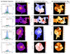 |
Fig. 1. Mapping results of our MUSE HzRGs sample. (a) Master Lyα spectrum (blue shaded histogram) extracted from a r = 0.5 arcsec aperture at the AGN position with best fit (solid dark magenta line). Red dashed curve shows the intrinsic Lyα from fitting, i.e. corrected for absorption. The vertical black bars above the emission line mark the positions of the H I absorbers. The yellow shaded region (if any) indicates the 5 wavelength pixel range excluded in the fitting due to the contamination from the 5577 Å sky-line. The flux density unit, Fλ, is 10−20 erg s−1 cm−2 Å−1. We also show the scaled He IIλ1640 Å spectrum extracted from the same position in green histogram. We scale the peak flux density of He II to 0.3 − 0.7 (varied for different targets) of the maximum peak flux density of observed Lyα spectrum in −1000 to 1000 km s−1. The Δv = 0 km s−1 is the systemic redshift based on He II or [C I] (Table 1, Kolwa et al. 2023). (b) Intrinsic Lyα surface brightness map. The flux in each tile is the integrated flux of the line emission corrected for absorption, i.e. total flux of the one or two Gaussians, see Sect. 3.2. The light blue circle shows the aperture where the Master spectrum is extracted from. Green triangles mark the positions of the radio lobes. We place a green bar linking the triangles on TN J0121+1320 to indicate the unresolved state of its radio emission. The length of the bar represents the linear size of the 3σ contour along the east-west direction. The white hatched regions are the ones where the flux uncertainty is higher than 50% of the fitted intrinsic flux. The white bar indicates the 50 pkpc at the redshift of the radio galaxy. The unit of the surface brightness is 10−16 erg s−1 cm−2 arcsec−2. We apply the same colour scale for all targets. (c) v50 map of the intrinsic Lyα nebula. The zero velocity used for each target is determined by the systemic redshift (Table 1). Green contours show the morphology of the radio jet in arbitrary values. The green cross mark the AGN position (Table 2). (d) W80 map of the intrinsic Lyα nebula. The black hatched regions on (c, d) are the same as (b). The purple hatched regions (in 4C+03.24 and TN J1338-1942) are manually excluded due to contamination from either foreground star or known companion (Arrow galaxy in the filed of MRC0316-257, see Vernet et al. 2017). We note that the colour scales for panels c and d are customised. The purple hatched area (if any) indicates the manually excluded region affected by foreground star or known Lyα emitter. |
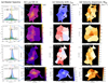 |
Fig. 1. continued. |
The known degeneracy between the H I column density and Doppler parameter in our fits (e.g. Silva et al. 2018a) does not affect the reconstructed intrinsic emission which is the focus of this work. We show the ‘Master Lyα spectrum’ extracted from a central 1″ aperture in Fig. 1a which presents how the intrinsic profile compares to the observed spectrum (see Sect. 4.1 for details).
We emphasise that the term ‘intrinsic Lyα emission’ throughout the work refers to the nebula Lyα emission corrected for intervening absorbers. The absorption troughs seen on the spectra (Fig. 1a) are due to the Lyα emission being absorbed by these neutral hydrogen gas clouds or shells along the line of sight. Under the aforementioned assumptions, a natural consequence is that the absorbers must be distributed across the whole projected extension of the nebula. The fact that we mostly observe these features continuously across the extent of the nebulae in most HzRGs indeed indicates they are coherent intergalactic-scale structures. This can be found in Figs. 2–4 where similar absorption features are seen in the selected spectra at larger distance (10s of kpc) away from AGN. Similar maps of the remaining sources are shown in Appendix C which are the ones have been previously published (Swinbank et al. 2015; Gullberg et al. 2016; Vernet et al. 2017; Falkendal et al. 2021; Wang et al. 2021b). Our approach is a common interpretation in studies of HzRGs. Conversely, such absorbers are not often seen in the Lyα nebulae of other quasars. This reinforces the interpretation that strong (radio-mode) feedback on intergalactic scales is needed to create such ‘shells’ of H I material. The use of a Gaussian as underlying intrinsic emission profile is supported both by observational and modelling works (e.g. Arrigoni Battaia et al. 2019; Chang et al. 2023). This could be a result of prior radiative transfer effects of Lyα (e.g. local scattering or scattering from the broad line region of the AGN Verhamme et al. 2006; Gronke & Dijkstra 2016; Gronke et al. 2016; Li et al. 2022). The radiative transfer modelling requires assumptions about the composition and geometry (and kinematics) of the gas near the AGN which is not the focus of this paper. Hence, we just assume the Gaussian shape of the Lyα (which could be due to the radiative transfer effects) and correct for the absorption along the line of sight to reconstruct the intrinsic emission on CGM scales. Incorporating radiative transfer calculations into the study of HzRGs Lyα nebulae is beyond the scope of this current work. Further developments of theoretical works are required (e.g. adding jet and resolving shells in simulations), and our dataset would be well suited for such studies. We therefore stress that the presented results are only valid for the stated assumptions that absorption rather than radiative transfer is primarily responsible for the line profiles. We discuss the limitation of this treatment in Sect. 5.1.
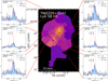 |
Fig. 2. Example for the intrinsic mapping of the Lyα nebula of TNJ0205+2242. The central panel shows the intrinsic surface brightness map of TNJ0205+2242 which is the same as Fig. 1b. The green cross and triangles mark the position of the AGN and jet lobes, respectively. In each of the side panel, we show the spectrum (blue shade histogram in normalised flux unit) extracted from the individual spatial bin whose number is labelled at the top left, and the best fit (dark magenta curve) and recovered intrinsic Lyα (dashed red line). The black vertical bars indicate the positions of the H I absorbers. |
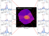 |
Fig. 3. Similar to Fig. 2, but for TNJ0121+1320. |
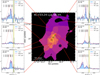 |
Fig. 4. Similar to Fig. 2, but for 4C+03.24. The red box marks the secondary southern K-band continuum emission peak (van Breugel et al. 1998, Sect. 4.2.4). The yellow shaded regions show the wavelength range excluded due to the 5577 Å sky-line. |
We note that the O V]λλ1213.8,1218.2 (O V]) line underneath the Lyα can affect the obtained flux especially in the nuclear region where the ionisation parameter (and metallicity) is higher (Humphrey 2019). In our pilot study (Wang et al. 2021b) of 4C+04.11, we found the contribution from O V] is negligible. Hence, we do not further include O V] in our line fitting. We leave the inspection to future work when data of metal lines (e.g. N Vλλ1238, 1243 which is found to be related with O V]) and high resolution spectra are analysed.
3.2.2. Fitting procedure
To reconstruct the intrinsic Lyα emission across the nebula, we fit each spectrum in each tessellation bin (see Sect. 3.1.2) following the procedure described in Sect. 3.2.1. We take into account the physical connection between neighbouring tiles by using the fit results of a previous connected bin as the starting parameters for the next bin (see Appendix A for details on the ordering). We determine the number of absorbers based on the Master spectrum where the S/N is the highest (Fig. 1a). We then use that same number of absorbers across the nebula, where the centroid, column density and Doppler parameter of absorbers are fitted in a given range (Appendix B). This assumption is supported by the profile shapes at the largest spatial extents (see Figs. 2–4 and also Appendix C). We note that the number of absorbers selected here may be incomplete but this has minor effects on the results of this paper: (i) the absorbers that impact most the intrinsic flux (i.e. spatially extended ∼10″ and having higher column density and/or larger Doppler parameter) are included; (ii) absorbers that seem to be ‘superfluous’ at the wings have only minor effects on the reconstructed flux where S/N is low (Fig. 2–4). Future work using high spectral resolution data will address these issues also taking into account that some of these absorbers have counterparts in metal lines covered by the MUSE data (e.g. N Vλλ1238, 1243 and C IVλλ1548, 1551 Kolwa et al. 2019; Wang et al. 2021b). We perform the fit in each bin using both one and two Gaussian emission line components and we choose the solution that minimises the reduced χ2. The fit is done using a least-squares method followed by a Markov chain Monte Carlo (MCMC, using the python package emcee, Foreman-Mackey et al. 2013) sampling. The uncertainties we report are either the direct output of the 1σ error by the MCMC or the propagated 1σ error. A detailed description of the fitting procedure is provided in Appendix B. We reiterate that we do not report any further parameters on the absorption features which will be analysed in future work in combination with higher spectral resolution data (e.g. Jarvis et al. 2003; Wilman et al. 2004; Kolwa et al. 2019, Ritter et al., in prep.). We present the results of this procedure for all of our sources in Fig. 1.
4. Results
4.1. Intrinsic mapping
In this section, we present the intrinsic maps (i.e. corrected for absorption) constructed following the fitting procedure described in Sect. 3.2. For each sources we show the Master spectrum together with its best fit in Fig. 1a as an example (Sect. 3.2.1). We also show the non-resonant He II spectrum extracted in the same aperture (green histogram, not continuum subtracted) which is used for systemic redshift (Δv = 0 km s−1, Table 1) determination. We note that there is no He II detected at the AGN position for 4C+03.24 (Sect. 4.2.4). In addition, to illustrate how fitting procedure works spatially (Sect. 3.2.2), the selected exemplar individual fits are shown in Figs. 2–4 (also see Appendix C).
The intrinsic Lyα surface brightness maps are shown in Fig. 1b on the same flux scale. Regions with larger fitting uncertainties (≳50%) that should be treated with caution are indicated by the overlaid hatched tiles. We report the total intrinsic Lyα luminosities (LLyα, int) of the nebulae in Table 2 and their maximum linear extent, dmax, in Table 3. Down to the surface brightness limit (Table 2), seven of our nebulae are extended over 100 pkpc with the largest being ∼347 pkpc (MRC0316-257). TNJ0121+1320 is the only target with nebula < 100 pkpc (∼72 pkpc). The total intrinsic surface brightness (LLyα, int) of the nebulae ranges from 2 to 29 × 1044 erg s−1.
HzRGs MUSE sample properties.
HzRGs nebulae properties.
To characterise the kinematic information of the intrinsic nebulae that are fitted with one or two Gaussians, we use a set of non-parametric emission line measurements (see e.g. Liu et al. 2013) derived from the cumulative line flux as a function of velocity Φ(v) defined as:
 (1)
(1)
where f(v′) is the flux density at v′. The often used v50 is the velocity where the cumulative flux reaches 50% of the total integrated value, Φ(v50) = 0.5Φ(∞). The v05, v10, v90 and v95 are defined similarly. The line width measurement, W80, defined in this context is W80 = v90 − v10. In case of single Gaussian fits, W80 is directly related to the FWHM and v50 is the Gaussian centroid.
The non-parametric velocity shift (v50) and line width (W80) of the nebulae are shown respectively in panels c and d of Fig. 1. The v50 maps do not show clear trend on larger scale (i.e. beyond the jet hot spots) for the whole sample. This is foreseeable given that (i) Lyα is a resonant line which is sensitive to scattering (i.e. it will not necessarily show the bulk velocity of the gas), and we only observe the last scattering surface; (ii) the size of the tile far from the centre is larger which could smear out potential velocity structures; (iii) the line emissions on several 10s of pkpc could trace the inflowing gas (or other gas components not governed by the host galaxy and/or kinematically related to the quasar outflow, e.g. Vernet et al. 2017). Within the extent of the radio jets, 3 targets (MRC0943-242, MRC0316-257 and TN J1338-1942) show tentative velocity gradients consistent with the jet kinematics (Sect. 2.1.3). For the line width maps, W80, 3 targets (4C+03.24, 4C+19.71 and TN J1338-1942) show a trend with the line being broader near the centre and becoming narrower outwards. There are some tiles on the periphery of the nebulae, for example the south-west tile of 4C+04.11, displaying larger W80 values (≳2500 km s−2). Except 4C+19.71, all targets show a line width of ∼800 − 2500 km s−1. For 4C+19.71, due to the strong 5577 Å sky-line located close with the observed Lyα peak wavelength, its line width should be treated as lower limit (≳600km s−1) especially for the tiles in the outskirts of the nebula.
We note that the non-parametric measurements used in this mapping are based on intrinsic (= absorption-corrected) line profiles which are determined through model fitting, same as Wang et al. (2021b). In Appendix C, we present the maps of observed surface brightness and flux ratio as supplementary material.
4.2. Radial profiles
4.2.1. Circularly averaged surface brightness radial profiles
In this section, we present the surface brightness radial profile of the eight Lyα nebulae. In order to compare our HzRGs to other quasar samples, we extract the surface brightness profile centred around the AGN in circular annuli. The annuli over which the profiles extracted are shown in Fig. D.1. We compute the surface brightness in each annulus as the mean of the surface brightness of each contributing spaxel weighted by the fraction of the spaxel area covered by the annulus. Table D.2 lists the extracted intrinsic profile values.
Figure 5 shows the radial profiles after correction for cosmological dimming and in comoving units for observed (upper panel) and intrinsic (lower panel, corrected for absorption) maps. The dashed lines in the upper panel represent the comparison quasar samples or single targets (an extremly red quasar and 2 radio-loud quasars from Lau et al. 2022; Vayner et al. 2023, respectively). The selected quasars are all observed by advanced IFU instruments (MUSE or KCWI) and cover a large range of redshift and physical properties. They are luminous radio-quiet quasars at z ∼ 3.2 quasar from Borisova et al. (2016; profiles from Marino et al. 2019), luminous type-1 quasars at z ∼ 3.17 from Arrigoni Battaia et al. (2019), luminous quasars at z ∼ 2.3 from Cai et al. (2019), high redshift quasars at z ∼ 6.28 from Farina et al. (2019) and luminous quasars at z ∼ 3.8 from Fossati et al. (2021). The quasar nebulae do not show so many absorption features as in our HzRGs and the studies were preformed without absorption corrections (Sect. 5.1). Nevertheless, since the comparison quasar samples are not corrected for absorption, we do not show them all again in our intrinsic profile (lower) panel. The two exceptions are Farina et al. (2019, hereafter F19) and Vayner et al. (2023; 7C 1354+2552, V22 7C). Those two are on the higher surface brightness end of the comparison samples, and we examine them quantitatively along with both the intrinsic and observed HzRGs profiles. We note that Vayner et al. (2023) fitted the Lyα absorbers from the spatially integrated 1D spectrum and found ∼1013.5 cm−2 for the column densities. For F19, there is not much evidence of absorption. Therefore, the comparison is legitimate. The best fit profiles to the observed Lyα nebulae of radio loud quasars in Arrigoni Battaia et al. (2019) are included in both panels of Fig. 5 which can be used as a reference between the two panels.
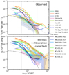 |
Fig. 5. Radial profiles of the Lyα nebulae extracted in circular annuli (Fig. D.1). For better comparison, we show the radial profile in comoving kpc (ckpc) and take the cosmological dimming into account by a factor of (1 + z)4, where z is the redshift of the target. The black dot-dashed curve and grey dotted line in both panels are the best fitted exponential and power law profiles of the Arrigoni Battaia et al. (2019) radio loud sample, respectively. The two vertical dotted lines mark the 50 and 300 ckpc, respectively. Upper panel: Radial profile of observed surface brightness map in thicker solid lines. In this panel, we also include the radial profiles of other quasar samples (dashed lines) for comparison: B16 – Borisova et al. (2016), AB19 – Arrigoni Battaia et al. (2019), C19 – Cai et al. (2019), Farina19 – Farina et al. (2019), Fossati21 – Fossati et al. (2021), L22 – Lau et al. (2022) and V22 – Vayner et al. (2023; two sources, 4C09.17 and 7C 1354+2552). When it is available, we show the range spanned by the 25th and 75th of the comparison sample radial profile as the shaded region around median profile in the same colour. The horizontal bars at the right-most indicate the observed surface brightness limits (scaled by area from Table 2) for each target in the same colour. Lower panel: Intrinsic radial profile in thicker solid lines. The shaded regions around each profiles indicates the uncertainty range of the surface brightness from fitting. In this panel, we show again the same profiles of F19 and V22 7C as in the upper panel for comparison. Our HzRGs are extended further with higher surface brightnesses (or flattening in some sources) at larger radii (∼300 ckpc) compared to other samples. |
Except for the extremely red quasar from Lau et al. (2022; which is also highly obscured), type-1 radial profiles are dominated by direct emission from bright AGN point source in the inner regions (∼50 ckpc or ∼10 pkpc). Hence, due to point spread function (PSF) subtraction, the inner-most radius covered in the comparison samples is limited to ∼50 ckpc in most cases (except Vayner et al. 2023). At larger radii, the contamination by the PSF should be negligible. Of the three single target profiles, V22 7C (7C 1354+2552 from Vayner et al. 2023) has the highest surface brightness. At a radius of ∼50 ckpc, the intrinsic surface brightness of our HzRG sample has a factor of 0.5 − 7 compared with V22 7C (7 of our targets are brighter). This source then shows a faster drop off compared with HzRGs. At the faint end corresponding to ∼300 ckpc (except TN J0121+1320), the HzRGs have a factor of 7 − 100 higher surface brightness than V22 7C. The profile of Farina et al. (2019) shows the highest surface brightness among the comparison samples. At ∼50 ckpc, the intrinsic HzRG profiles are still a factor of 1.1 − 15 (or 4 − 40 at ∼400 ckpc, except TN J0121+1320) brighter than the 75th percentile of Farina et al. (2019). These indicate that our eight observed HzRG have some of the brightest known Lyα nebulae (Sect. 2.1). We note that the jet compression is also known to result in high Lyα nebula luminosity (e.g. Heckman et al. 1991a,b). Compared to quasars with similarly deep observations (i.e. avoiding the surface brightness detection limit), our HzRG sample generally maintains a high surface brightness out to larger radii (5 out of 8 > 500 ckpc). We note again that the detected extent of our nebulae will have similar range even if adopting other detection methods than the ones in this paper (Sect. 3.1). For example, Gullberg et al. (2016) reported the similar extend Lyα nebula in MRC0943-242 with less exposure time. Vernet et al. (2017) detected the nebula of MRC0316-257 > 700 ckpc based on visual detection. Swinbank et al. (2015) found the > > 500 ckpc nebula of TN J1338-1942 with (or even without) a simpler binning algorithm. Hence, we are sure that the detection of the ≳500 ckpc nebulae in our sample based on our method is robust. However, we do caution that this sample is not representative since they are selected to have bright and extended Lyα emission. The profiles of MRC0943-242, MRC 0316-257 and TN J1338-1942 show a flattening at rAGN > 200 ckpc. For the comparison samples, their profiles drop off monotonically and drop below detection limit at radii smaller than our HzRGs. The lowest surface brightness of HzRG intrinsic profiles is ∼1 × 10⁻¹⁵ erg s−1 cm−2 arcsec−2 (MRC0316-257, corrected for cosmological dimming) which is higher than the faint end of the quasar samples by a factor of 5 − 40 (not at similar comoving distances). These indicate that we are observing some of the most extend Lyα nebulae, in two cases (MRC0316-257 and TN J1338-1942) even extending beyond the field of view of MUSE. By simply comparing our intrinsic profiles to the exponential and power law fits of Arrigoni Battaia et al. (2019), we find that the inner part of HzRGs profiles are exponential-like (especially MRC0943-242 and TN J1338-1942) while extended parts show power law decline. We note, however, that the exponential part is affected by seeing smearing.
If we do not correct for the Lyα absorption and instead measure at the observed radial profiles (Fig. 5 upper panel), 5 of the HzRGs are still brighter than the comparison samples, but by a lower factor of ∼2 − 4 (∼2 − 6) at radii of ∼400 (∼50) ckpc compared to the 75th percentile of Farina et al. (2019). Comparing the results from intrinsic and observed profiles, this suggest that the quasar samples may miss a non-negligible amount of flux (≳5) due to uncorrected for absorption.
The radial surface brightness profiles of the comparison samples are extracted from a fixed velocity or wavelength range, for example ±2000 km s−1 in Cai et al. (2019), 30 Å in Arrigoni Battaia et al. (2019) and ±500 km s−1 in Farina et al. (2019). Considering the redshift difference between these samples, the integration range adopted are consistent. For our study, particularly for the observed radial profile, our extraction is based on the v05 and v95 which are determined based on intrinsic fitting (Sect. 4.1). In this way, we can minimise the uncertainties coming from the observed line width difference, for example between the emission lines in the vicinity of the host and outskirts of the nebula. Our velocity range (v05 and v95) used is basically the value of W90 which has the range of ∼800 − 2700 km s−1 for all tiles of all targets. Nevertheless, we conduct a check by extracting observed circular radial profiles through integration of 30 Å around the systemic redshift of our targets for comparison. The results vary by ∼ ± 10% in each annulus to the profiles in Fig. 5 (from v05 and v95), especially for emissions at > 50 ckpc where the line width is narrower comparing to the centre. The 30 Å extracted profile could be 40% less than the v05 − v95 extraction in the centre regions (wider line width) for high-redshift targets where the fixed wavelength range in observed frame corresponds to a narrower rest frame range. Hence, to alleviate this problem brought by the difference in line width and redshift range spanned by our sample, we keep the v05-to-v95 extraction. As for the intrinsic radial profile, it is redundant to integrate from a narrower range when we can have the direct fit results for the integrated Lyα line. We show the flux ratio between the intrinsic and observed maps in the same velocity range in Appendix C which can be used as a proxy for scaling between the two profiles. Therefore, the different wavelength (velocity) ranges used when extracting radial profiles for our study and comparison quasar samples will not bring additional discrepancy besides the relatively large surface brightness value in our sample.
4.2.2. Directional surface brightness profiles
Since the shapes of our Lyα nebulae are asymmetric (Sect. 4.3), the radial profiles extracted in Sect. 4.2.1 smear out direction-dependent features. For instance, several HzRG Lyα nebulae display features aligned with their radio jets, such as having higher line width and elongated morphology along the jet axis (e.g. van Ojik et al. 1997; Villar-Martín et al. 2003; Miley et al. 2004; Zirm et al. 2005; Humphrey et al. 2007; Morais et al. 2017). Hence, in this section, we study the radial profile of the intrinsic Lyα emission along the direction of the radio jet which could exert a kinematical and/or electromagnetic influence on the surrounding gas. Due to the limited S/N, we split our nebulae into two half parts (approaching and receding, Appendix D) along the jet direction and extract the surface brightness profile in each direction using the same annuli as Sect. 4.2.1. Figure 6 shows these directional profiles. We also show the position of the jet hot spot for the receding (red) and approaching (blue) side with vertical dashed lines2. Qualitatively speaking, the surface brightness on the receding side is higher than on the approaching side within the radio jet extent for most of our sources (except 4C+03.24 and 4C+04.11). In three sources, the receding jet hot spot is closer to the AGN: MRC0316-257, TN J0205+2242 and TN J1338-1942. This result was first reported by McCarthy et al. (1991) where the authors found that the line emission is brighter in HzGRs on the side with shorter radio jet. They interpreted this as a large-scale asymmetry in the density of gas on either side of the nucleus: the denser gas absorbs more ionising radiation resulting in brighter emission lines, while the radio jet is more contained as it travels more slowly through the denser medium.
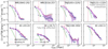 |
Fig. 6. Surface brightness radial profiles for approaching (blue squares) and receding (red circles) directions along the jet axis. The dotted curves in corresponding colours show the exponential+power law fits for the two directional profiles. We also include the fits for the circularly averaged profile in solid magenta lines. In each panel, the magenta shaded region mark again the same uncertainty range for the intrinsic surface brightness profile as Fig. 5. The solid green curve is the normalised radial profile of a star extracted up to 2″ (the one in the FoV of MRC0316-257 is extracted from a round galaxy due to no available star) showing the PSF (Table 1). The vertical dashed lines indicate the distances of the jet hot spots in corresponding colours. The profile along the receding side of the jet is brighter than along approaching side for most sources within the extent of the jets except 4C+03.24 and 4C+04.11. This may indicate different gas density distribution (see Sect. 4.2.2). We also identify flatting of the profile at ≳100 ckpc for MRC0943-242, MRC0316-257 and TNJ1338-1942 which may related to nearby companions (see Sect. 5.4). |
4.2.3. Fitting the surface brightness profiles
To quantify the shape of the profiles, we fit the circularly averaged intrinsic profile and two directional intrinsic profiles with a piecewise function split into an exponential for the inner part and power law for the outer part. This can be mathematically represented by
 (2)
(2)
where rh is the scale length of the exponential profile, rb is the distance at which the inner and outer profiles separate and Ce and Cp are normalisation parameters for exponential and power law profiles, respectively ( ). The determination of the piecewise function is motivated by previous studies of quasar Lyα nebula (e.g. Arrigoni Battaia et al. 2019; Cai et al. 2019; den Brok et al. 2020) which fit the profile by either power law or exponential. We also test to fit our profiles use only one of the two functions. The single profile, however, cannot fit some targets well. For example, the reduced χ2 are high (> 20) for MRC0943-242, MRC0316-257 and TN J1338-1942 with the single-function fit. We therefore fit all of the profiles with the piecewise function for consistency. Figure 6 shows the fits and Table D.3 presents the fitted parameters.
For most of our targets, the two directional surface brightness profiles are similar to the circularly averaged profile. One exception is the approaching side of MRC0316-257 which has ∼1 dex lower than the receding side. This could be an extreme case of uneven Lyα emitting which may trace the different gas distribution. In Fig. 6, we also show the distance of the jet hot spots on both directions (Appendix D). There is no correlation between the distance of the jet hot spot and rb (nor rh). As Sect. 4.2.1 described, our HzRGs are high in surface brightness (large Ce); the reasons for this include (i) our sample is composed of HzRGs with bright Lyα emission, (ii) our profiles are absorption corrected, (iii) the quasar surface brightness is extracted from a fixed wavelength range (Sect. 4.2.1). The exponential shape is also seen in other quasar samples, for example Arrigoni Battaia et al. (2019), Farina et al. (2019), den Brok et al. (2020) and Lau et al. (2022). The rh values derived for our sample are mostly < 20 pkpc (Table D.3) which is consistent with the quasars. This suggests a similarity between the central (high surface brightness) part of HzRGs to other quasars (type-1 radio-loud and radio-quiet, type-2 radio-quiet), despite the high surface brightness in our sample. We note that the PSF-subtraction of quasar samples and resolution effects will impact the inner part to the profile. We further discuss the power law declining (flattening) part of our nebula in Sect. 5 combining the information from nebular morphology (Sect. 4.3).
4.2.4. Radial profiles of kinematic tracers
It is of interest to study how the nebula kinematics changes radially which may offer evidence of outflow and/or inflow (e.g. Humphrey et al. 2007; Swinbank et al. 2015; Vernet et al. 2017). We stress that it is beyond the scope of this work to separate different Lyα kinematics emission components (e.g. systemic and outflow) which will be inspected through high resolution spectroscopic data. Hence, we adopt the v50 and W80 parameters to measure the overall kinematics of the line emitting gas (Sect. 4.1). We caution that the kinematics derived in this way may be biased, for example if there are several gas components with different kinematics but on similar flux levels.
In Fig. 7, we show the directional radial profiles of v50 (Fig. 1c) and W80 (Fig. 1d), respectively. The profiles are extracted in a similar way as the directional surface brightness in Sect. 4.2.2 by splitting the map into two halves (approaching and receding). The v50 (W80) value shown at each radius is averaged in the corresponding annulus. Within the extent of the radio jet hot spots (vertical dashed lines), MRC0943-242, MRC0316-257, TN J0205+2242 and TN J1338+1942 show evidence of jet-driven outflows (e.g. Nesvadba et al. 2008, 2017a) if we ignore the absolute v50 value but focus on the relative gradient. That is to say the velocity shift at the approaching side is higher than the receding side. For these four targets, we overplot a solid green line to show the fit of the velocity radial profile within the radio jet extent in Fig. 7. The same velocity gradient is also identified in He II for MRC0943-242 (Kolwa et al. 2019), MRC0316-257 (Appendix E) and TN J1338+1942 (Swinbank et al. 2015). There is no other evidence from the v50 of ordered gas bulk motion for the overall sample. This further suggests that Lyα is an unreliable tracer of kinematics at least on 10s to 100s pkpc scale in HzRGs. We note that the tessellation implemented, especially for tiles with larger size (∼5 arcsec2) which are usually located in the low S/N region away from the host galaxy, may smear out potential kinematic features. One possible consequence of combining different kinematic components is broadening of the line width. This may be the case for the receding side of MRC0316-257 and both sides of TNJ0121+1320 and 4C+04.11. In general, the W80 does not show an increasing trend towards larger rAGN. However, if the line width decreases intrinsically away from the AGN, this will counteract the broadening which makes it difficult to check the impact of smearing. Therefore, we mark the regions with rAGN > 5″ on the kinematic radial profile using grey shade to flag the possible high uncertainty in Fig. 7.
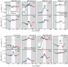 |
Fig. 7. Directional v50 and W80 profiles for approaching (blue squares) and receding (red circles) sides along the jet axis extracted from the intrinsic maps (i.e. corrected for absorption, Fig. 1cd). The vertical dashed lines indicate the distances of the jet hot spots (blue for approaching, red for receding, Appendix D). We note that the radio emission of TN J0121+1320 is unresolved. The grey shaded regions are > 5 arcsec from the host galaxy. The data points in the shaded regions should be treated with caution given the large tile size may smear kinematic structures. The horizontal black dotted line in the v50 panel marks the 0 km s−1 derived from systemic redshift. The dashed horizontal black line in the v50 panel of 4C+03.24 indicates the velocity shift of Hβ redshift (zHβ ≃ 3.566, −1100 km s−1 with respect to the systemic redshift; Nesvadba et al. 2017b) with respect to its systemic used in this paper (Table 1, see text). We note that the range of the x-axis is customised for each target and that the W80 is shown in logarithmic scale. We show a zoom-in view of the central part of the v50 profiles of MRC 0316-257 and TN J1338-1942 in the insets. For MRC 0943-242, MRC 0316-257, TN J0205+2242 and TN J1338-1942, we mark the fit to the v50 profiles within the jet hot spots (vertical lines) in green lines to guide the eye of the evidence of nebula velocity gradient following jet kinematics. In general, there is no clear evidence of a trend in bulk motion identified for the whole sample. For some targets (4C+03.24, 4C+19.71 and TN J1338-1942), W80 decreases with increasing radial distance which may indicate that the jet is disturbing the gas. |
If we assume that the bulk of the gas resides in the potential well of the radio galaxy, we expect to see the Lyα emission gas centred around systemic velocity, at least in the vicinity of the AGN. Offsets of the v50 levels at rAGN ∼ 0 ckpc from 0 km s−1 (based on systemic redshift, Table 1) are identified for most of our targets which may be due to the aforementioned bias from different kinematic components and scattering of Lyα photons. The most noticeable case is 4C+03.24 which has an offset of ∼900 km s−1. We note that its systemic redshift (Table 1) is based on [C I](1–0) emission (Kolwa et al. 2023) due to lack of He II from the AGN position in the MUSE data (Fig. 1a). This offset can be eased if we use the redshift of Hβ, zHβ ≃ 3.566, reported by Nesvadba et al. (2017b) as zero velocity. It is marked in black dashed horizontal line in the v50 panel of 4C+03.24 in Fig. 7. This corresponds to −1100 km s−1 with respective to the systemic velocity shift used in this paper. We caution that, however, the Hβ was not exclusively extracted at the AGN position (radio core). There is also a known jet-gas interaction in the south of the AGN (see bend of the radio jet contours in Fig. 1b and also van Ojik et al. 1996). From the K-band image (van Breugel et al. 1998), we can find a second continuum emission peak in the south. The position of this emission peak is marked by the red square in Fig. 4. Given these pieces of evidence, we propose that there is a companion galaxy at zHβ ≃ 3.566 in the south of our radio galaxy (z = 3.5828). If there is (or was) an interaction between these two galaxies, the companion may have deprived gas from the AGN resulting in a gas poor AGN host (no detection of He II and less molecular gas detected at the AGN position, Kolwa et al. 2023). The companion then becomes sufficiently massive and gas-rich to deflect the jet. Therefore, the Lyα nebula of 4C+03.24 may trace the CGM of the companion galaxy. Scheduled JWST data (Wang et al. 2021a) will offer a clearer view of this particular situation.
For the W80 radial profiles in Fig. 7, we can first identify that most of the HzRGs have high W80 even at larger radii (∼1500 km s−1). The exception is 4C+19.71 whose measurement is affected by sky-line residuals (Sect. 4.1). The W80 reported here is similar to FWHM (especially at large radii, > 100 ckpc or ≳22 pkpc) where most of our fit are done with a single Gaussian (Sect. 3.2). In 4C+03.24, 4C+19.71 and TN J1338-1942, we can see a clear radial decrease of W80 along both directions. This may be related to results found in Villar-Martín et al. (2003) who observed a Lyα FWHM drop off at distance beyond the extent of the radio jets in a sample of HzRGs (including MRC0943-242) using deep Keck long slit spectroscopy. In our study, however, we firstly do not find such a decrease in all targets. The grey shaded regions (rAGN > 5″) should be treated with caution. We note that the FWHM in Villar-Martín et al. (2003) was derived without correction for absorption. Since we see a high spatial coverage of absorbers (Figs. 2–4), the correction indeed helps with recovering the close-to-intrinsic gas kinematics at large radii. In Fig. D.2, we show the position-velocity diagram extracted based on our observed and intrinsic surface brightness maps along the jet as a direct comparison with the long slit spectroscopic study. Although it resembles the detection of Villar-Martín et al. (2003) at first glance, we note that this is due to the tessellation and the contrast between high surface brightness and low surface brightness part.
By considering both the radial profiles from v50 and W80, we can generally find that the profiles within the jet extents have behave differently compared to the profiles outside the jet extent. This again suggests the jet is disturbing or entraining the Lyα emitting gas. There are unclear signs of kinematics other than outflows or inflows seen mostly at larger radial distance ∼300 ckpc. For example, MRC0943-242 stays relatively flat (for both v50 and W80), while MRC0316-257 has a decrease in W80 followed by an increase beyond the jet extent on the receding side. We reiterate that in this analysis we do not distinguish between (potential) different kinematics components by using v50 and W80 to quantify the overall velocity shift and line width. This may bring bias of the measured values. Additionally, the measured kinematics farther from the AGN are averaged from larger annulus (e.g. projected area of ∼4 × 10⁴ pkpc2 at ∼60 pkpc or ∼300 ckpc) which will bring another bias. We point out again that we use grey shade to mark the data > 5″ from the centre which has larger tile size. Nevertheless, we note that the detected W80 of ∼103 km s−1 (and abrupt velocity shift) at large radii (∼300 ckpc) in some of the profiles could be caused by the fact that the detected Lyα emission is dominated by emission halos of nearby companions (e.g. Byrohl et al. 2021).
4.3. Morphology of the nebulae
The nebula morphology is related to the ionising sources, gas dynamics and galaxy environment (Byrohl et al. 2021; Costa et al. 2022; Nelson et al. 2016). Especially when the Lyα nebulae (in our sample) can probe the CGM gas beyond 100 pkpc. By visual inspection, we observe that the shape of our Lyα nebulae are asymmetric (e.g. Fig. 1). In this section, we study quantitatively the nebula morphology. We first focus on the whole nebula by introducing the morphology quantification measurements (ellipticity, nebula orientation and offset between nebula centroid and AGN position) in Sect. 4.3.1 and compare with other samples in Sect. 4.3.2. Then, in Sect. 4.3.3, we study how the nebula asymmetry changes with radial distance for individual targets. We also report the detected morphology correlations between different measurements (i.e. offset between AGN and nebula centroid position, nebula ellipticity and nebula linear size) in Sect. 4.3.4. These shed light on how the central quasar and nearby companions can affect the observed nebula morphology. Finally, in Sect. 4.3.5, we show the non-random oration of jet axis and its relation with the elongated direction of nebula which hints at the CGM gas distribution.
4.3.1. Morphology quantification measurements
To quantify the asymmetry, we introduce a set of morphology measurements. Arrigoni Battaia et al. (2019) used flux-weighted asymmetry measurements for the Lyα nebulae which is sensitive to the high surface brightness part. In other works (e.g. den Brok et al. 2020), an unweighted asymmetry measurement was adopted for better studying the extended structure of the nebulae (sensitive to the morphology of the whole nebula). To better characterise the morphology of our HzRGs and perform comparison with other samples, we analyse the asymmetry with both the flux-weighted and flux-unweighted methods.
First, we follow Arrigoni Battaia et al. (2019) and calculate the flux-weighted asymmetry, αweight (see Arrigoni Battaia et al. 2019, for the definition). This quantifies the asymmetry of the nebula in two perpendicular directions. Together with the asymmetry measurement, we also obtain the flux-weighted position angle θweight, which we use as an indicator for the elongation direction of the nebula after converting it to the same reference system as the radio jet axis (i.e. angle measured east from north). The flux-weighted nebula centroid (centre of the nebula) is also computed. We note that the intrinsic flux and its uncertainty are used as weight to measure these three parameters and to calculate the corresponding uncertainties, respectively. We also derive the asymmetry measurement weighted by observed flux for comparison. Second, to compare with flux-unweighted asymmetry reported for other quasar samples (e.g. Borisova et al. 2016; den Brok et al. 2020), we calculate the αunweight following den Brok et al. (2020). In this context, we also derive θunweight (flux-unweighted position angle) to examine the jet-nebula relation with respect to the entire nebula. Figure 8 visualises the weighted (nebula centroids and θweight) and unweighted (θunweight) parameters on the eight nebulae.
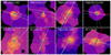 |
Fig. 8. Zoom-in intrinsic surface brightness maps (Fig. 1b) of the HzRGs sample to 15 × 15 arcsec2 (or ∼110 × 110 pkpc2) around the central AGN (blue cross). In each panel, the blue+red and green solid lines indicate the direction of, and perpendicular to, the radio jet. The blue (red) colour represents the direction of the approaching (receding) jet. The white dashed line shows the flux-weighted position angle of the nebula (θweight). The white dotted line shows the unweighted position angle of the nebula (θunweight). The white star indicates the intrinsic flux-weighted centroid of the Lyα nebula. The flux weighted measurement is sensitive to the morphology of the high surface brightness part of the nebula. The unweighted measurement quantifies the morphology of the whole nebula. We find that nebula is elongated along the jet axis for most of HzRGs. |
In Lau et al. (2022), the authors compared morphology of different quasar samples. Following their comparison, we convert the aforementioned asymmetry measurement (for both flux-weighted and unweighted), α, to an intuitive elliptical asymmetry measurement (or ellipticity)  . For eweight → 0, the nebula is closer to round shape and vice versa. Table 3 reports the morphological parameters of our sample. Since the absolute flux-weighted centroid position and θweight (and θunweight) are irrelevant, we report the projected distance between the nebula centroid and the AGN position (dAGN − neb) and the difference in angles between θweight (and θunweight) and the jet position angle (|θweight − PAradio| and |θunweight − PAradio|), respectively. The jet position angle (PAradio) is shown in Fig. 8 and listed in Appendix D.
4.3.2. Comparison of nebula asymmetry with other quasar samples
Figure 9 presents the ellipticity measurements as a function of their nebula Lyα luminosity for our targets and other quasars (Borisova et al. 2016; Arrigoni Battaia et al. 2019; Cai et al. 2019; Mackenzie et al. 2021; den Brok et al. 2020; Sanderson et al. 2021; Lau et al. 2022). We note that the LLyα for comparison samples are not corrected for absorption. Part of the comparison samples are also used in Sect. 4.2.1 for surface brightness radial profile analysis. We point out the newly included ones here: faint z ∼ 3.0 type-1 from Mackenzie et al. (2021) and type-2 AGN at z ∼ 3.4 from den Brok et al. (2020) and z ∼ 3.2 from Sanderson et al. (2021). The reason why they are not included in radial profile analysis is that they do not add new information.
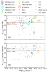 |
Fig. 9. Relation between Lyα nebula luminosity and asymmetry measurement. (a) Flux-weighted Lyα nebula elliptical asymmetry measurement versus nebula luminosity, LLyα. We show the intrinsic flux-weighted ellipticity (eweight) in larger open symbols for our targets versus their intrinsic Lyα luminosity. We also show the observed flux-weighted ellipticity eweight, obs for our targets versus their observed Lyα luminosity in smaller filler symbols. The small grey symbols are data of comparison targets (AB19 – Arrigoni Battaia et al. 2019, C19 – Cai et al. 2019 and L22 – Lau et al. 2022). We mark the median flux-weighted (not corrected for absorption) ellipticity, 0.72, of type-1s with the horizontal dashed line. We also show the median eweight, 0.69, of radio-loud type-1 quasars from Arrigoni Battaia et al. (2019) in red horizontal dash-dotted line. (b) Flux-unweighted Lyα nebula elliptical asymmetry measurement versus LLyα. The larger symbol are measurements for our HzRGs while the grey symbols are comparison targets (type-1s: B16 – Borisova et al. 2016, L22 – Lau et al. 2022 and M21 – Mackenzie et al. 2021; type-2s: dB20 – den Brok et al. 2020 and S21 – Sanderson et al. 2021). We mark the median eunweight for type-1s (0.69) and type-2s (0.80) in solid and dashed horizontal lines, separately. The eweight is sensitive to the morphology of the high surface brightness part of the nebula while the eunweight quantifies the morphology of the whole nebula. We note that for e → 0, the nebula is closer to round shape and vice versa. At the bottom right, we show the median uncertainty of the intrinsic LLyα for our sample in logarithmic scale, 0.04. The ellipticity for our sample are higher compared to the other quasars for both high surface brightness part and whole nebula. There is no clear evidence that the nebula ellipticity correlates with luminosity. |
The HzRGs from our sample are measured to be asymmetric for their high surface brightness emission region (median eweight ≈ 0.78). Compared to the Arrigoni Battaia et al. (2019) and Cai et al. (2019) samples, our HzRGs are consistent in asymmetry measurements and on the higher end of their distribution (type-1 median eweight ≈ 0.72, dashed horizontal in Fig. 9a). The eweight of radio-loud type-1s from (Arrigoni Battaia et al. 2019) have a median of 0.69 which is even lower than the value of all type-1 targets (Arrigoni Battaia et al. 2019; Cai et al. 2019). This indicates that the radio emission in type-1 does not disturb the gaseous nebula as in our HzRGs at least along the plane of the sky. This further suggests that orientation is a critical factor (Sect. 5.3). By comparing the intrinsic flux-weighted and observed flux-weighted elliptical asymmetry measurements, we find the eweight can vary significantly (e.g. MRC 0316-257 and 4C+04.11). For MRC0316-257, we can already identify its asymmetric morphology through visual checking (Fig. 1). There is also a large error bar associated with the intrinsic flux-weighted ellipticity. Hence, the morphology of MRC0316-257 is more towards the asymmetric end. The large difference between its intrinsic and observed eweight could be due to the absorption correction elevates the flux difference between the high and low S/N regions thus gives more weight to the central nebula. As for 4C+04.11, this could be due to the potential over-correction of the absorption in the low S/N regions given we use nine absorbers across the nebula (Sect. 3.2, 5.1). However, we point again that the absorption is necessary to reconstruct the intrinsic flux given that the absorption features across the nebula were observed (e.g. Swinbank et al. 2015; Wang et al. 2021b).
Our HzRGs have a median eunweight ≈ 0.70 which is lower than the measurement of type-2s and relatively consistent with the type-1s (median eunweight ≈ 0.80 and ≈0.69, respectively, Borisova et al. 2016; den Brok et al. 2020; Sanderson et al. 2021; Mackenzie et al. 2021). The ellipicity of the comparison type-2s is calculated from five sources which may not be representative. We note that there is a large scatter in the eunweight measured for our sample with four clustered around the type-2s and other four below the median eunweight of type-1s. This result could be biased by the implemented analysis methods (i.e. detection map and tessellation, Sect. 3.1): (i) the construction of the detection map may smooth out the nebula asymmetry at larger radii (lower S/N); (ii) the tessellation results in lager bin sizes along the direction perpendicular to the radio jet (lower surface brightness and S/N, Sect. 5.5) which shapes the nebula morphology to be more round. This brings more effects of the quantification of the entire nebula. Hence, the HzRGs nebulae will likely have larger eunweight (i.e. more asymmetric) than the quantified value. In spite of that, we can conclude that at least half of our sample, together with the type-2s, distribute at the most asymmetric end in terms of the whole nebula. The rest has the possibility to be skewed to higher eunweight. Our HzRGs have diverse properties and are not necessarily representative for the entire HzRGs population. Inspection for individual targets is required.
As for the LLyα, our HzRGs host the most luminous Lyα nebula compared with other quasar types. This is due to the following: (i) sample selection3; (ii) absorption correction; and (iii) quasar PSF subtraction of comparison samples (Sect 4.2.3).
We further compare our HzRGs to the ERQ from Lau et al. (2022). In Fig. 9, both the eweight (0.44) and eunweight (0.69) of L22 are lower than the measurements from HzRGs. Its LLyα is also lower than our HzRGs by ∼2 orders of magnitude. This confirms that the nebula of this EQR is type-1 like but highly obscured (e.g. Lau et al. 2022). Since it is the only source of this type, we do not further discuss it.
4.3.3. Asymmetry radial profile
To further quantify the morphology of individual nebula as a function of distance from the AGN, we follow den Brok et al. (2020) and decompose our HzRGs intrinsic surface brightness using Fourier coefficients, ak(r) and bk(r):
![Mathematical equation: $$ \begin{aligned} \mathrm {SB}_{Ly\alpha } (r,\theta )= \sum _{k=0}^{\infty }\left[a_{k}(r)\cdot \cos (k\theta )+b_{k}(r)\cdot \sin (k\theta )\right]\text{,} \end{aligned} $$](/articles/aa/full_html/2023/12/aa46415-23/aa46415-23-eq5.gif) (3)
(3)
where SBLyα(r, θ) is the surface brightness at given polar coordinate (r, θ). The coefficients ak(r) and bk(r) are defined as:
 (4)
(4)
The detailed description can be found in den Brok et al. (2020). Then we combine ak(r) and bk(r):
 (5)
(5)
We measure the radial dependence of the asymmetry (i.e. how much it deviate from a circular shape) of the nebulae by using the ratio between kth and 0th modes, ck(r)/c0(r). In practise, only the first three modes are used since the higher mode coefficients are much smaller (den Brok et al. 2020). Figure 10 shows the radial profiles of this asymmetry measurement (represented by (c1/c0)2 + (c2/c0)2 on the y-axis) for our HzRGs. The larger the value, the more asymmetric the morphology shift from circular shape at a given radial distance. We also include type-2 measurements from den Brok et al. (2020; 4 quasars) and Sanderson et al. (2021) as comparison. The type-1 sample from Borisova et al. (2016; which is quantified in den Brok et al. 2020) is also shown. Our HzRGs generally show an increase of the asymmetry as a function of radial distance (some have a smaller secondary peak at ≲50 ckpc) and a steep rise to > 1.5 (7 out of 8) at ∼250 ckpc. The most noticeable exception is MRC0316-257 which has a secondary peak (∼0.8) at ∼50 ckpc (∼14 pkpc). This flux-weighted measurement confirms the large difference we observed in the high surface brightness part of the directional profiles of MRC0316-257 in Fig. 6. As we already stated in Sect. 4.2, the detected extent of our HzRGs (≳400 ckpc) are larger than the comparison quasars (∼300 ckpc). If we limit the comparison to the largest extent (∼250 ckpc) reached by the type-1s from (Borisova et al. 2016), we find that our HzRGs are similar in radial asymmetry measurements. Specifically, both have a relatively flat profile to ∼200 ckpc which followed by a shallow rise to the value of ∼0.5. However, in Sect. 4.3.2 (Fig. 9) we find that the HzRGs ellipticity is larger than type-1s. Together with the radial asymmetry profile in this section, we can conclude that the asymmetry of the nebulae associated with HzRGs and type-1s are different due to structures at larger radial distance (> 250 ckpc) from AGN. This is also suggested by den Brok et al. (2020). Although we caution the large W80 at large distance in Sect. 4.2.4 and mark the region with r > 5 arcsec in grey in Fig. 7, we can still find that most targets have at least W80 ∼ 103 km s−1. This may indicate that these structures are likely disturbed and not ‘quiescent’ gas in the Cosmic Web (Sect. 5). From the comparison with type-2s (den Brok et al. 2020; Sanderson et al. 2021, which also have a steep rise), we find that the radial asymmetry of our HzRGs rises at larger radial distance (≳250 ckpc) and reaches higher asymmetry value (> 1.5 compared with ∼1.4 of type-2s). At least one of the radial asymmetry measurement (Cdfs 15, with the furthest extent rAGN ∼ 300 ckpc) from den Brok et al. (2020) shows an indication of continuous rising up to the detection limit (1 hour integration with MUSE); we cannot rule out the possibility that this target may show a similar trend as the HzRGs with deeper observations.
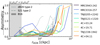 |
Fig. 10. Radial profiles of the surface brightness Fourier decomposition (asymmetry measurement). The c0, c1 and c2 are the 0th, 1st and 2nd modes Fourier decomposition coefficients of the surface brightness radial profile, respectively (see den Brok et al. 2020, for definition). The (c1/c0)2 + (c2/c0)2 is a measurement of nebula asymmetry along the radial distance from the AGN. Our HzRGs are shown in solid colour lines. rAGN is the radial distance measured from the central AGN. For comparison, we include the same measurements for the 4 nebulae of type-2 quasars from den Brok et al. (2020; grey dashed lines) and the type-2 from Sanderson et al. (2021; grey dot-dashed line). We also include the type-1 measurements from Borisova et al. (2016; dotted line represents the median and shaded region marks the 25th and 75th percentile, quantified by den Brok et al. 2020). The vertical shaded region is the 0.75 arcsec (∼25 ckpc) range affected by median seeing of our sample (the radial distance where the type-1 PSF is affected is ∼50 ckpc, see den Brok et al. 2020). The morphologies for most of the HzRGs nebulae are round (symmetric) ≲100 ckpc and become asymmetric at larger radial distances ∼100 ckpc (see text). |
4.3.4. Morphological correlations
In Fig. 11, we compare the eweight (ellipticity that is sensitive to high surface brightness nebula) and dmax (maximum nebula extent) against dAGN − neb (offset between AGN and nebula flux-weighted centroid). For a consistent comparison for the unweighted measurements, we should use the unweighted offset (centroid) and the unweighted ellipticity. We note that the calculation of unweighted ellipticities, eunweight, assumes that the centre of nebula corresponds to the AGN position (den Brok et al. 2020). It would involve large uncertainties if we calculated the flux-unweighted nebula centroids (i.e. the geometric centre of the nebula) which are entirely depended on the spaxel distribution from our detection maps (Sect. 3.1.1). Hence, we report only the correlation between flux-weighted ellipticity and offset, and use it as a proxy of the nebula even though they are more sensitive to the high surface brightness part.
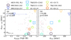 |
Fig. 11. (a) Intrinsic flux-weighted ellipticity (sensitive to the morphology of the high surface brightness part of the nebula), eweight, versus distance offset between nebular centroid and AGN position, dAGN − neb. The typical uncertainty of dAGN − neb (σdAGN − neb = 0.4 pkpc, Table 3) is shown at bottom left. (b) Maximum Lyα nebula linear extent, dmax, versus dAGN − neb. In both panels, we give the Spearman correlation measurements for our sample at the top left (the star superscript indicates the correlation is calculated excluding MRC 0316-257 in panel a). We also include the data from Arrigoni Battaia et al. (2019) in both panels in grey (radio quiet) and pink (radio loud) dots. We note that the Arrigoni Battaia et al. (2019) sample shown in this figure is incomplete to concentrate on the relation for our targets. There are positive correlations detected for eweight–dAGN − neb and dmax–dAGN − neb. |
The (r-value, p-value) of Spearman’s correlation coefficients are (0.89, 0.007) and (0.88, 0.004) for the eweight versus dAGN − neb and dmax versus dAGN − neb relations. We note that due to the large uncertainties of eweight for MRC0316-257, we exclude it from the correlation measurement. From the r-values and p-values, we can conclude that eweight and dmax are both correlated with dAGN − neb. This suggests that the more asymmetric and more extended nebulae have larger offsets between AGN position and nebular centroid. We also include the Arrigoni Battaia et al. (2019) sample for comparison. The (r-values, p-values) of the eweight − dAGN − neb relation for the Arrigoni Battaia et al. (2019) whole sample and radio-loud targets are (0.3, 0.02) and (0.3, 0.4), respectively, implying no strong correlations. The (r-values, p-values) of the dmax − dAGN − neb relation for the Arrigoni Battaia et al. (2019) sample and the radio-loud targets are (0.4, 0.003) and (0.4, 0.1), respectively, suggesting a moderate correlation in their whole sample but not in their radio-loud target. This indicates that the radio-loud type-1s are different from our radio-loud type-2s HzRGs. We revisit these correlations in Sect. 5.
4.3.5. Jet-nebula position angle distribution
We present the distribution of the |θ − PAradio| (Sect. 4.3.1, Table 3) in Fig. 12. Both the flux-weighted and unweighted measurements are shown which are sensitive to high-surface brightness parts and the entire nebulae, respectively. Figure 12 shows that most HzRGs have |θ − PAradio|< 30°. A similar result was reported by Heckman et al. (1991b). This observation is consistent with the scenario proposed by Heckman et al. (1991b,a) that the compression of the gas by the radio jet results in brighter emission along the jet. We discuss the indications behind the alignments further in Sect. 5.5. The exception is 4C+04.11 which has both large |θweight − PAradio| (81.4°) and |θunweight − PAradio| (45.3°), indicating different conditions that in the other targets (such as inflows, Sect. 5.6). In TN J0121+1320 we find a flux-unweighted angle difference of 72.1°. Given its round Lyα nebula morphology and compact radio emission, there is a large uncertainty in angle difference measurement and we do not discuss this source separately. If we assume the observed angle difference is equally distributed from 0 − 90°, the probability for us to find 7 (or 6) targets in a sample of 8 with |θ − PAradio|< 30° is only 0.2% (1.7%) using bimodal distribution.
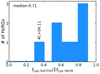 |
Fig. 12. Distribution of the angle difference between nebular position angle and radio jet position angle, |θ − PAradio|. The blue histogram shows the number distribution of flux-weighted angle difference, |θweight − PAradio| (sensitive to high surface brightness nebula morphology). The magenta histogram represents the unweighted measurements, |θunweight − PAradio| (quantifying the morphology of the whole nebula). The values are presented in Table 3. We mark the obvious outliers in the two distributions in corresponding colours. This shows that most of our HzRGs have their Lyα nebula elongated along the jet axis. |
5. Discussion
5.1. Absorption correction and radiative transfer
We stress that the analysis of our sampled Lyα nebulae in this paper is under the idealised assumptions stated in Sect. 3.2.1. Specifically, we interpret the trough features in the Lyα spectra as absorption features by the neutral hydrogen gas surrounding the radio galaxy. In this section, we discuss the limitations and possible caveats of this treatment for reconstructing the intrinsic Lyα flux along with the possible effects brought by radiative transfer.
Under our assumptions, the absorbing gas is located in between the observer and the last scattering surface of Lyα photons along the line of sight. The intrinsic Lyα flux reconstructed under our treatment is thus assumed to be the one after radiative transfer processes have shaped the Lyα nebula, and is approximated by a Gaussian profile. We also assume the absorbed Lyα photons in the absorbers to be ‘lost’ rather than continuing their resonant scattering path within the nebula; this may happen when photons are absorbed by dust and re-emitted as infrared thermal emission, or preferentially scattered away from the line of sight due to a particular geometry (see Sect. 3.2.1). The latter may occur because photons originating from the backside of the galaxy have a higher chance to be absorbed by dust when transiting the host galaxy (Liu et al. 2013). These absorbers can be interpreted as intervening low column density gaseous shells (e.g. van Ojik et al. 1997; Swinbank et al. 2015; Kolwa et al. 2019). The fact that most of the absorbers are located in the blue wing of the Lyα profile as well as the fact the trough of the main absorber is often seen across several tens of kpc scales supports this idea (see Fig. 1a, and TNJ0205+2242 in Fig. 2, see also TNJ1338-1942 in Fig. C.4 and e.g. Wang et al. 2021b).
The situation may be different when we encounter embedded absorbers which are supposed to be closer to the source of Lyα photons (i.e. central AGN in our case). This leaves the trough (or ‘main absorber’) at around the systemic redshift of the AGN as predicted by radiative transfer studies (e.g. Verhamme et al. 2006). Even though the scales probed in those simulations are different (CGM scale versus sub-kpc), this might be the case in some of our targets, for example MRC0943-242 and TNJ0121+1320 (Figs. 3 and C.1). Therefore, one consequence of our absorption treatment (with ‘lost’ photons) is that we may double-count Lyα photons that are resonantly scattered to the wing and/or other directions by redundantly adding more when correcting for absorption. We implemented a simple test for checking the double-counting effect, which takes advantage of the IFU nature where slit or spaxel loss effects are compensated by photons resonantly scattered in the neighbouring spaxels. Specifically, we summed all individual spectra into one and reconstruct the intrinsic flux for this single spectrum (fLyα, full FOV); this value removes the IFU information, but should be a good measure of the total value emanating from the nebula in the observer’s direction. This is then compared to the sum of individually constructed intrinsic flux in each tile (Fig. 1b, ΣfLyα, tile fit). Figure 13 shows the result, where a value of 1.0 is expected if our treatment is fully accurate. Instead, we observe a median value of 0.71 for our sample, indicating that there may be double-counting of photons. However, several effects may also contribute to this. First, our assumption of a Gaussian shape for the intrinsic profile may not be accurate, as prior radiative transfer effects may have created troughs and boosted the line wings (Verhamme et al. 2006). A future paper presenting high spectral resolution UVES observations of our sample will help to better model the profiles (Ritter et al., in prep.). Second, the assumption that all absorbers extend across the entire nebula may also be oversimplified. While many absorbers are indeed seen on 10s (or 100s) of kpc scales for our targets (Figs. 2–4 and also Appendix C), there may be exceptions.
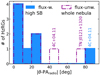 |
Fig. 13. Distribution of fLyα, full FOV/ΣfLyα, tile fit for our HzRGs. The fLyα, full FOV is the intrinsic Lyα flux resulted from fitting the spectrum summed over the entire FOV. The ΣfLyα, tile fit is the summation of the intrinsic Lyα flux in each tessellation bin (Fig. 1b). The smaller the value, the more likely the Lyα photon is being double-counted when correcting for absorption. 4C+04.11 is the one with the smallest ratio which may also indicate over-correction (Appendix B). |
The Lyα nebula properties of the type-1 (and radio-quiet type-2) sources in the comparison samples are derived without correcting for absorption. They are still good comparison samples given that not many absorption features are detected in them (e.g. Arrigoni Battaia et al. 2019). This fact alone is already an indication that there may be an environmental differences between the nebulae of HzRGs and other quasars. Alternatively, this difference may related to intrinsic differences between different AGN types.
Overall, it is likely that both the absorption and radiative transfer effect are working together shaping the Lyα profile. Our analysis assumes that the absorption correction is the dominant factor.
5.2. Lyα nebula and AGN unification model
The unification model of AGN (e.g. Antonucci 1993) proposed that the fundamental difference between type-1 and type-2 is due to the different orientation of the obscuring dusty torus (ionisation cone). Specifically, the ionisation cone of type-1s is more aligned with the observed line of sight than in type-2s.
Within this unification model, we assume that the power of AGN is on a similar level for type-1s and type-2s and that their gaseous nebulae therefore have similar distributions and masses. If we further assume that the ionising photons are primarily produced by the AGN, then the nebulae should have similar morphologies and luminosities. In this picture, the Lyα nebulae are elongated along the direction of the ionisation cone and have a ‘rugby-ball’ shape. For type-1s, the ionisation cone would be pointing towards the observer resulting in a rounder nebula morphology. For type-2s, the ionisation cone would aligned along the plane of the sky resulting in the observed elliptical morphology. Evidence for such a scenario was indeed reported in He et al. (2018) using ionised gas nebulae but for local AGN and on small scales (sub-kiloparsec to kiloparsec).
Using both the eweight (sensitive to the high surface brightness nebula) and eunweight (whole nebula) quantifying the ellipticity of the nebula, we find that the HzRGs (and other radio quiet type-2s) are more asymmetric than the type-1s in Sect. 4.3.1. This observation agrees with the AGN orientation unification model. The orientation of type-1s probably still vary in a range which causes the large range of the ellipticities. The AGN luminosity and dark matter halo mass (gas distribution) can also play an important role in shaping the observed morphology (Fig. 9).
With the jet axis indicating the direction of the ionisation cone (Drouart et al. 2012) and the alignment between the jet axis and the Lyα nebula (at least in the high surface brightness part where the photons of AGN are presumably dominating the ionisation, Sect. 4.3.5 and Fig. 12), we argue that the AGN orientation between type-1s and type-2s (HzRGs) can explain the observed morphological difference. The evidence for this claim comes mostly from the observed ellipticity distribution (Fig. 9): the eweight (median 0.69, Sect. 4.3.2) for radio-loud type-1s (Arrigoni Battaia et al. 2019) are lower than our HzRGs (median 0.78), which is consistent with the jet (ionisation cone) pointing more towards observers in type-1s. By checking the available radio maps of these radio-loud type-1s (e.g. Fig. B1 in Arrigoni Battaia et al. 2019), we indeed find that they have compact radio morphology (i.e. not the two-side jet like HzRGs) suggesting that the jets are aligned more perpendicular to the plane of the sky. We note that TNJ0121+1320 also has a compact radio morphology (i.e. not having two-side jet) and the lowest eweight (0.66) and eunweight (0.48) in our sample (more consistent with type-1 results, see Fig. 1 and 9) which again fits the unification model.
A similar explanation was also suggested by den Brok et al. (2020) based on Lyα nebula studies of type-2 quasars (also included as comparison sample in this paper). den Brok et al. (2020) suggested that the orientation difference based on unification model can explain the nebula morphology at radial distance ≳40 pkpc. Using the same radial asymmetry measurement in Fig. 10 (Sect. 4.3.3), we also find large nebula asymmetries at ≳40 pkpc (∼200 ckpc) in our HzRGs following den Brok et al. (2020) type-2s. den Brok et al. (2020) found more symmetrical morphologies for their type-2s at small radial distances < 30 pkpc that are more similar to type-1s. den Brok et al. (2020) suggested that additional ionising sources other than the AGN (e.g. star forming processes) may contribute to this observation and smear out the differences between type-1 and type-2 at such small radii. As for our HzRGs, the jet-gas interaction at ≲20 − 30 pkpc (∼100 ckpc) could be a reason for the observed high eweight shown in Fig. 9a (compared to type-1s) and the reason of the small rise (showing higher asymmetry compared to type-2s) in the radial asymmetry measurement at ∼60 ckpc in Fig. 10.
5.3. The role of Lyα resonant scattering
As presented in Sect. 4.1 and 4.3, Lyα nebulae around our HzRGs are extended in size (≳150 pkpc) and are asymmetric in shape. Interestingly, there is a correlation between the maximum nebula extent dmax (eweight: ellipticity measurement that is sensitive to high surface brightness nebula) and the offset between AGN position and nebulae’s flux-weighted centroid dAGN − neb (Sect. 4.3.4). This correlation may also reflect our findings regarding the surface brightness and kinematic radial profiles in Sect. 4.2.1 and 4.2.2, such as the exponential shape of the surface brightness in the inner nebula and high W80 value. The resonant nature of Lyα photons may be related to this observation.
Villar-Martin et al. (1996) first proposed the idea of resonant scattering being related to the observed extended nebula emission around HzRGs. In simulations, Costa et al. (2022) found that the scattering of Lyα photons, regardless of the powering source, could result in an offset between the luminosity centroid of the nebula and the quasar position (dAGN − neb). This offset can vary depending on the line of sight and can reach ∼15 pkpc. Such offsets are consistent with what we find (Table 3). The authors also found that scattering can shape the nebula into a more asymmetric morphology (eweight → 1). This depends on the gas distribution of neutral hydrogen and observed line of sight as described in Costa et al. (2022). Given the common case that gas density is the highest on galaxy scales, and that we target type-2 AGN, we expect the Lyα photons to scatter out to larger projected distances rather than travelling directly towards the observer. Such a scenario may explain our observed correlation in Fig. 11 between eweight and dAGN − neb. Specifically, when the scattering is more efficient, we may observe the nebula to be more asymmetric and more extended, at least in the high surface brightness regime.
Resonant scattering has the potential to shape the observed inner parts of the radial profiles (surface brightness and kinematics) and the morphology correlations. The inner part (luminous) of the surface brightness radial profiles have an exponential shape (Sect. 4.2.1). This gradual change in surface brightness and profile slope at smaller radii is suggested to be due to scattering (Costa et al. 2022). The high W80 values out to radius of ∼50 pkpc (or ∼230 ckpc, Sect. 4.2.4) could also be related with efficient scattering (Fig. B1 in Costa et al. 2022). The velocity shift of the nebulae can also be complicated due to scattering at the similar radial distance (Fig. B1 in Costa et al. 2022) which is the case of our v50 (Fig. 1c, Sect. 4.1). As shown by the stellar radial profiles (Fig. 6), the impact of seeing cannot be fully responsible for the exponential shape at smaller radii. For the observed kinematics, the jet (which is not included in the simulations) may also play a role here. We overlay the jet hot spot distances on the radial profiles (Figs. 6 and 7). Qualitatively, the v50 and W80 show different behaviours within and outside the extent of the jet hot spots at least for some targets (e.g. MRC0316-257). We note that the distances marked by the vertical lines are measured from the brightest radio emission positions, that is, the full extent of jet is even larger (Appendix D). The decrease of W80 at large radii (≳100 pkpc) observed in some targets (e.g. TN J1338-1942) is, beyond the scope of the Costa et al. (2022) simulations but could be related to the (unvirialised) cosmic web.
In the framework where scattering significantly impacting the observed Lyα properties, Costa et al. (2022) furthermore predicts that Lyα nebulae of edge-on AGN should have lower surface brightness, larger dAGN − neb, more asymmetric shape and flatter surface brightness profiles in the centre. Most of the predictions agree with our observations except for lower surface brightnesses, which could be due to our selection criteria and/or jet impact. We note that the analysis of Costa et al. (2022) has been done without correcting for absorption which is reason of the discrepancy.
The orientation (Sect. 5.2) may be the reason for the moderate dmax − dAGN − neb relation seen in the sample of (Arrigoni Battaia et al. 2019; i.e. the orientation spans a large range within the sample). The larger the viewing angle (i.e. the more edge-on we are observing the AGN, assuming unification model, Antonucci 1993), the more extended the nebula is expected to be, because both sides of the nebula will be observed. The nebula is expected to become more asymmetric and have larger dAGN − neb as Costa et al. (2022) predicted. The study of type-2 quasars (e.g. den Brok et al. 2020; Sanderson et al. 2021) also found that the difference in nebula morphology when comparing to type-1s is related to AGN orientation. Interestingly, for our HzRGs, we do find a relatively strong correlation between dmax and dAGN − neb despite the expectation that most HzRG are observed under similar, large viewing angles, (i.e. close to edge-on). All of our targets have clear two-sided radio lobe morphology (except TN J0121+1320) and none of them shows clear signs of broad-line emission or significant contamination by a bright point-like source in the centre (see also Drouart et al. 2012, and Sect. 2.1.3).
5.4. Large-scale environment: Nearby Lyα emission halos
Byrohl et al. (2021) studied Lyα emission halos and their relation with environmental factors using TNG50 simulation. They found a flattening in the Lyα halo surface brightness radial profile at large radial distances (≳30 pkpc). The authors attributed this to the contribution of scattered photons from nearby halos (companions). In Sect. 4.2 (and 4.2.3), we show that the profiles of three of our targets (MRC0943-242, MRC0316-257 and TN J1338-1942) also have an obvious flattening at large radii (Fig. 6). Coincidentally, these targets are known to live in dense environments (on Mpc scale, e.g. Venemans et al. 2007). All of this indicates that our nebulae are ‘contaminated’ by Lyα halos associated with nearby companions (e.g. Gullberg et al. 2016). In addition, the observed surface brightness radial profile of MRC0316-257 (Fig. 5) at large radii, shows a decline followed of a rise, and is a factor of five brighter than the 2σ surface brightness limit (16 for the intrinsic) which indicate an extra source of Lyα photons. The filamentary Lyα emitting comic structures are observed on Mpc scales (e.g. Umehata et al. 2019; Bacon et al. 2021). Bacon et al. (2021) discussed the possibility that the diffuse Ly-alpha emission is powered by low mass galaxies not directly detectable in the deep (140 hours) MUSE observation.
These results provide additional evidence that the detected nebula connects with the emission halo of companions. If this is the case, we should revisit the dmax − dAGN − neb in Sect. 4.3.4. When a quasar resides in a dense environment, its apparent size will likely be impacted by neighbouring Lyα nebulae. This ‘contamination’ from nearby companions will likely be more related to the large-scale structure and independent of the orientation of the central (quasar) halo. In other words, the hidden parameters behind the dmax − dAGN − neb (eweight − dAGN − neb, Sect. 4.3.4, Fig. 11) relations may be related to the distribution of the companion emission halos. Contamination from neighbouring halos will result in the centroid of the nebula being offset from the AGN position and cause a more asymmetric nebula morphology. The nearby companions can be the disturbing sources resulting in the ∼1000 km, s−1 line width seen at ∼100 pkpc (W80, Fig. 7).
The radial asymmetry profiles of our targets have a larger value than type-1s and type-2s (Fig. 10) at larger radii, which is unlikely to be entirely due to the AGN orientation (Sect. 4.3.3). This can now be explained by the impact and contamination of nearby companions at 100s of pkcp. We point out that the type-2 from Sanderson et al. (2021) has a projected size of 173 pkpc, a nebula centre offsets from the AGN of ∼17 pkpc and high ellipticity (0.8). This source is also found to have nearby companions (∼60 pkpc). The difference of the radial asymmetry profiles (Fig. 10) and surface brightness profiles between this source and our HzRGs may be related to the jet (or large-scale gas distribution, Sect. 5.5).
The stellar masses of the galaxies studied in Byrohl et al. (2021) are in the range of 8.5 < log10(M⋆/M⊙) < 10 which is approximately 1 − 2 orders of magnitude lower than the stellar masses of our HzRGs, implying lower dark matter halo masses, as well. Such lower masses may explain the difference in the level of Lyα surface brightness where the flattening of the profiles is observed: in the simulations by Byrohl et al. (2021) the flattening happens at a surface brightness level of ∼10−20 erg s−1 cm−2 arcsec−2 (e.g. their Fig. 7) while we observe it to happen at a level of ∼10−18 erg s−1 cm−2 arcsec−2). The dark matter halo mass difference can also explain the different radial distance at which the companion emission dominates (∼30 pkpc in Byrohl et al. 2021, versus ∼40 pkpc, Table D.3). We note that we use the rb, the radius at which surface brightness radial profile changes from exponential to power law (Sect. 4.2.3), as the distance where nearby halos start to significantly impact the surface brightness.
The ≳100 pkpc extents of the Lyα and the dense environments of HzRGs (Wylezalek et al. 2013) suggest that nearby halos may contribute to our observations (Byrohl et al. 2021). However, this also suggests that our CGM study is ‘contaminated’ by sources other than the radio galaxy. For this paper, we exclude obvious emission of clearly detected companions (e.g. ‘Arrow galaxy’ Vernet et al. 2017). A systematic census of the companion galaxies in the MUSE HzRG fields will be reported in a future paper.
5.5. Gas distribution on large scales
So far, we have focussed our discussion on morphological measurements sensitive to the high-surface brightness part of the Lyα nebulae and plausible explanation of environmental effect on ∼100 pkpc scales. It is likely that the jet shapes the nebula in the vicinity of the quasar to align with the jet axis (skewed distribution of |θweight − PAradio| towards values < 30°, Fig. 12) through interaction with the gaseous medium. Beyond the extent of the jets, we use |θunweight − PAradio| (which is equally sensitive to the whole nebula) to inspect the relation between the jet axis and halo asymmetry.
While it is unlikely that the jet plays a major role shaping the morphology of the large-scale halo, Eales (1992) suggested that the observed direction of the radio jet is the result of an inhomogeneous gas density. When a jet is launched along the direction of higher gas density (e.g. nH ∼ 10−2 cm−3), the jet ‘working surface’ (hot spots) will leading to brighter radio emission. Such a scenario would introduce a bias in observing jets preferably along directions of higher densities in flux-limited samples and we might expect a correlation between the morphology of a large-scale halo and radio jet axis. Our observations presented in Figs. 11 and 12 is in agreement with such a scenario.
The detection of molecular gas in HzRGs along the jet axis but beyond hot spots provides further evidence (< 20°, which suggests the jet runs into filament of cold gas Emonts et al. 2014). If this direction indeed traces a filament of the cosmic web (e.g. West 1991; Umehata et al. 2019; Bacon et al. 2021) with a higher density of companion galaxies, then this is also in agreement with the discussion presented in Sect. 5.4. Humphrey et al. (2007) found evidence of infalling CGM gas on to the HzRGs which bridges the radio galaxy and to the large-scale (IGM) gas. If the CGM gas is being accreted onto the central HzRGs through these higher density distributions, it would reflect the scenario proposed by Humphrey et al. (2007).
5.6. Evidence of capturing inflow from the cosmic web
The relatively large |θ − PAradio| (81.4° and 45.3° for weighted and un-weighted, respectively) detected in 4C+04.11 is inconsistent with other targets (see Fig. 12). This suggests that the nebula of 4C+04.11 is elongated in the east-west direction on both small (< 20 pkpc, scope of jet) and large scales (≳20 pkpc, Sect. 4.3.1 and 5.4). The tile with the largest distance from AGN position (# 74, Fig. A.9) has a filamentary like structure. There is no known evidence that 4C+04.11 resides at the centre of a dense cluster-like environment (e.g. Kikuta et al. 2017) which makes it unlikely that the asymmetry is caused by contamination of nearby halos as discussed in Sect. 5.4.
High velocity shocks (≳100 km s−1, Allen et al. 2008) can heat the gas which will then cool by radiating UV photons. Shocks could be caused by inflows and power the observed Lyα emission. We estimated the dark matter halo of 4C+04.11 is of the order of MDM ∼ 1013 M⊙ from it stellar mass, M⋆ ∼ 1011 M⊙ with an empirical M⋆ − MDM relation (Wang et al. 2021b). The surface brightness measured in the farthest tile #74 is ∼1.2 × 10⁻¹⁷ erg s−1 cm−2 arcsec−2 which is similar to (or slightly higher than) the simulated value from Rosdahl & Blaizot (2012). We converted our measurement to z = 3 which is redshift reported in the simulation. Our measurement and the simulation are consistent given that dark matter halo of 4C+04.11 is likely more massive than the one in the simulation (MDM ∼ 1012 M⊙).
Given the estimated dark matter halo mass, the virial radius and virial velocity can then be calculated as rvir ∼ 100 kpc and vvir ≃ 580 km s−1. From the centre of the tile #74, we can derive its distance to the central AGN as ∼60 kpc. We note that this is the projected distance averaged for spaxels in the tile. The actual distance of the filament could be farther. Even though it is closer, Nelson et al. (2016) simulated gas accretion into 1012 M⊙ halos at z = 2 and found that the accretion flow structure can remain filamentary within rvir (∼0.5rvir). The projected v50 (velocity offset) of tile #74 is −536 km s−1 which is consistent with vvir. Thus, our measurements for the projected distance of the tile and its velocity offset are consistent with a scenario where the Lyα emission in tile #74 may be tracing shock driven by inflows. If the distance we observe is indeed < rvir, then the post-virial accretion could be more complicated with multi gas phase components and fragmentation involved (e.g. Cornuault et al. 2018). The broad line width of 4C+04.11 at large radii (Fig. 7) may indicate the disturbed nature of the presumed accretion flow.
The discussion in this section based on the |θ − PAradio| and morphology of bin #74 of 4C+04.11. While the angle difference is a clear outlier in the sample, the tile shape may depend on the implemented method for nebula extent (Sect. 3.1.1). However, we checked the Lyα narrow band image (6690 Å to 6707 Å) directly collapsed from the data cube and confirm the indication of emission from this region. As for the nearby potential emission (north to bin #74, Fig. A.9), we confirm by spectral extraction that there is no S/N> 3 detection. Even if the Lyα emission is detected in this additional region, it would still be consistent with the accretion scenario. Complex filamentary structures are seen in simulations (see Rosdahl & Blaizot 2012, and their Fig. 7) for accretion in higher mass dark matter halo. Nevertheless, we caution that this analysis only considers one possibility. As the data are near the detection limit, deeper observation are needed before more conclusive results can be derived.
6. Conclusions
In this paper, we study the intrinsic Lyα nebulae around a sample of eight high-redshift radio galaxies using optical IFU observations obtained with MUSE. We link our observations to results from the literature for other quasars (mainly type-1 quasars) at similar redshifts.
We have developed a new method to measure the maximum extent of the nebulae with an improved sensitivity to low surface brightness emission. We have also developed a new method to tessellate the Lyα maps (Sect. 3.1). We have detected the Lyα emission at scales ≳100 pkpc from the central AGN, down to an observed surface brightness of ∼2 − 20 × 10−19 erg s−1 cm−2 arcsec−2.
We summarise our results as follows: The Lyα emission line profiles of all sources are affected by multiple and deep absorption troughs out to the edge of the nebulae. We have corrected for this H I absorption (Sect. 3.2) and constructed maps of the intrinsic Lyα (Sect. 4.1) emission and also measured the kinematic properties of the spatially resolved Lyα emission.
We first investigated radial dependencies of the surface brightness, velocity shift, and velocity width of our sample. We found that circularly averaged profiles of the intrinsic (absorption-corrected) Lyα surface brightness are brighter and more extended than type-1 quasar samples (Sect. 4.2.1). We did not find major differences when we investigated the radial profiles along the approaching and receding direction of the radio jets, respectively (Sect. 4.2.2). The surface brightness radial profiles can generally be described by an exponential drop-off for the inner high surface brightness part and a power law for the more extended part (Sect. 4.2.3). We did not find evidence of ordered gas bulk motion from the v50 radial profile (Sect. 4.2.4). For four targets, the v50 profiles at radii within the jet hot-spot range show a similar gradient as the jet-driven outflow (Fig. 7). The W80 profiles show relatively large values (≳1500 km s−1, Fig. 7, Sect. 4.2.4) at all radii and three targets show that a decrease beyond the distance of jet hot spots is indicative of jet-gas interactions.
We quantitatively studied the morphology of the HzRG nebulae (for both observed and intrinsic emission) and compared our results to other quasar samples (uncorrected for absorption, Sect. 4.3). We found that our nebulae are, in general, more asymmetric than nebulae of type-1 quasars and that they are more similar to type-2 quasars (Sect. 4.3.2), although, our sampled sources differ in their measure of asymmetry as a function of the radius (Sect. 4.3.3). Furthermore, we found that the more asymmetric and larger the nebulae are, the greater the offset between the centroid of the nebulae and AGN positions (dmax − dAGN − neb and eweight − dAGN − neb in Sect. 4.3.4, Fig. 11).
Lyα is a complicated emission line that can be heavily affected by absorption and resonant scattering which, as we demonstrated, needs to be accounted for. Assuming type-1 and type-2 quasars have similar intrinsic shapes for their nebulae, the difference of the nebulae asymmetry morphology between our sample and other quasars can be explained using the AGN unification model where the orientation of the ionisation cone is the fundamental parameter (Sect. 5.2). Resonant scattering of the Lyα emission can result in the observed dmax − dAGN − neb and eweight − dAGN − neb relation in our sample and partially explain the shape of the radial profile and the kinematic profiles (Sect. 5.3). We also found evidence in our HzRGs that the extended nebulae are affected by Lyα emissions from nearby companions (Sect. 5.4) and that CGM gas has a higher density distribution along a specific direction, which is coincident with the direction of the radio jet (Sect. 5.5). There is also a possibility that, in our observations, we captured inflows from the cosmic web (Sect. 5.6).
In this paper we have shown that measurements of Lyα nebulae around high-redshift AGN can act as a probe of the environment of AGN and their host galaxies. We have found fundamental differences between the extended ionised nebulae of different types of quasars at cosmic noon and beyond. Due to its resonant nature, it is a challenge to use Lyα as a tracer of gas kinematics especially out to the ∼100 pkpc scales. Nevertheless, Lyα line observations offer some insight into the state of CGM gas at a time when it is simultaneously being impacted by more than one physical mechanism (e.g. quasar outflow, jet-gas interaction, and cosmic inflow). These kinds of observations will be particularly useful for future simulation works. The MUSE data only reveal the tip of the iceberg. In upcoming papers, the H I absorbers will be reported together with the high-resolution spectroscopy data. In addition, all of the UV emission lines covered by MUSE will be studied in detail and this will provide crucial information on the ionisation, metallicity, and AGN feedback in the quasar nebulae. Furthermore, scheduled JWST observations will be available for four HzRGs in our sample and this will provide unprecedented details of the AGN and host galaxy connection on scales of ≲1 kpc (∼0.05″).
We note that this mask is only used in this process to eliminate the impact of the Lyα signal on ZAP. The detection map for determining the maximum extent of the Lyα nebula is described in Sect. 3.1.1.
We note that the radio emission of TN J0121+1320 is unresolved. The ‘jet size’ represented by the vertical lines are linear size of the 3σ contour along the east-west elongation of the radio map.
Distance ratio,  , is the ratio between the sum of the radii, r1 + r2, of the two tiles (estimated by
  , where A is the area of the tile) and the distance between the geometric centre of the two tiles, d1, 2.
For this case, we follow the procedure in Wang et al. (2021b) and fix the positions of five absorbers on the blue low S/N wing to the value determined from the Master spectrum.
Acknowledgments
We would like to thank Bjorn Emonts and Zheng Cai for valuable discussion which improved this work. This work uses the NASA’s Astrophysics Data System and a number of open source software other than the aforementioned ones such as Jupyter notebook (Kluyver et al. 2016); matplotlib (Hunter 2007); SciPy (Virtanen et al. 2020); NumPy (Harris et al. 2020); Astropy (Astropy Collaboration 2018); and LMFIT (Newville et al. 2016). B.G. acknowledges support from the Carlsberg Foundation Research Grant CF20-0644 ‘Physical pRoperties of the InterStellar Medium in Luminous Infrared Galaxies at High redshifT: PRISM- LIGHT’. M.V.M. acknowledges support from grant PID2021-124665NB-I00 by the Spanish Ministry of Science and Innovation/State Agency of Research MCIN/AEI/ 10.13039/501100011033 and by “ERDF A way of making Europe”. G.N. acknowledges funding support from the Natural Sciences and Engineering Research Council (NSERC) of Canada through a Discovery Grant and Discovery Accelerator Supplement, and from the Canadian Space Agency through grant 18JWST-GTO1. P.L. (contract DL57/2016/CP1364/CT0010) is supported by national funds through Fundação para a Ciência e Tecnologia (FCT) and the Centro de Astrofísica da Universidade do Porto (CAUP).
References
- Adam, G., Rocca-Volmerange, B., Gerard, S., Ferruit, P., & Bacon, R. 1997, A&A, 326, 501 [NASA ADS] [Google Scholar]
- Ahumada, R., Prieto, C. A., Almeida, A., et al. 2020, ApJS, 249, 3 [Google Scholar]
- Allen, M. G., Groves, B. A., Dopita, M. A., Sutherland, R. S., & Kewley, L. J. 2008, ApJS, 178, 20 [Google Scholar]
- Andrae, R., Schulze-Hartung, T., & Melchior, P. 2010, ArXiv e-prints [arXiv:1012.3754] [Google Scholar]
- Antonucci, R. 1993, ARA&A, 31, 473 [Google Scholar]
- Arrigoni Battaia, F., Hennawi, J. F., Cantalupo, S., & Prochaska, J. X. 2016, ApJ, 829, 3 [NASA ADS] [CrossRef] [Google Scholar]
- Arrigoni Battaia, F., Hennawi, J. F., Prochaska, J. X., et al. 2019, MNRAS, 482, 3162 [NASA ADS] [CrossRef] [Google Scholar]
- Astropy Collaboration (Price-Whelan, A. M., et al.) 2018, AJ, 156, 123 [Google Scholar]
- Bacon, R., Accardo, M., Adjali, L., et al. 2010, SPIE, 7735, 131 [Google Scholar]
- Bacon, R., Vernet, J., Borisova, E., et al. 2014, The Messenger, 157, 13 [NASA ADS] [Google Scholar]
- Bacon, R., Piqueras, L., Conseil, S., Richard, J., & Shepherd, M. 2016, Astrophysics Source Code Library [record ascl:1611.003] [Google Scholar]
- Bacon, R., Mary, D., Garel, T., et al. 2021, A&A, 647, A107 [NASA ADS] [CrossRef] [EDP Sciences] [Google Scholar]
- Basu-Zych, A., & Scharf, C. 2004, ApJ, 615, L85 [NASA ADS] [CrossRef] [Google Scholar]
- Best, P. N., Röttgering, H. J. A., & Longair, M. S. 2000, MNRAS, 311, 23 [NASA ADS] [CrossRef] [Google Scholar]
- Bicknell, G. V., Sutherland, R. S., van Breugel, W. J. M., et al. 2000, ApJ, 540, 678 [NASA ADS] [CrossRef] [Google Scholar]
- Binette, L., Kurk, J. D., Villar-Martín, M., & Röttgering, H. J. A. 2000, A&A, 356, 23 [NASA ADS] [Google Scholar]
- Bolatto, A. D., Wolfire, M., & Leroy, A. K. 2013, ARA&A, 51, 207 [CrossRef] [Google Scholar]
- Borisova, E., Cantalupo, S., Lilly, S. J., et al. 2016, ApJ, 831, 39 [Google Scholar]
- Byrohl, C., Nelson, D., Behrens, C., et al. 2021, MNRAS, 506, 5129 [NASA ADS] [CrossRef] [Google Scholar]
- Cai, Z., Cantalupo, S., Prochaska, J. X., et al. 2019, ApJS, 245, 23 [Google Scholar]
- Cantalupo, S., Lilly, S. J., & Haehnelt, M. G. 2012, MNRAS, 425, 1992 [NASA ADS] [CrossRef] [Google Scholar]
- Cantalupo, S., Arrigoni-Battaia, F., Prochaska, J. X., Hennawi, J. F., & Madau, P. 2014, Nature, 506, 63 [Google Scholar]
- Cappellari, M., & Copin, Y. 2003, MNRAS, 342, 345 [Google Scholar]
- Carilli, C. L., Röttgering, H. J. A., van Ojik, R., Miley, G. K., & van Breugel, W. J. M. 1997, ApJS, 109, 1 [NASA ADS] [CrossRef] [Google Scholar]
- Chambers, K. C., Miley, G. K., & van Breugel, W. 1987, Nature, 329, 604 [NASA ADS] [CrossRef] [Google Scholar]
- Chang, S.-J., Yang, Y., Seon, K.-I., Zabludoff, A., & Lee, H.-W. 2023, ApJ, 945, 100 [NASA ADS] [CrossRef] [Google Scholar]
- Christensen, L., Jahnke, K., Wisotzki, L., & Sánchez, S. F. 2006, A&A, 459, 717 [NASA ADS] [CrossRef] [EDP Sciences] [Google Scholar]
- Cigan, P. 2019, Astrophysics Source Code Library [record ascl:1909.002] [Google Scholar]
- Cornuault, N., Lehnert, M. D., Boulanger, F., & Guillard, P. 2018, A&A, 610, A75 [NASA ADS] [CrossRef] [EDP Sciences] [Google Scholar]
- Costa, T., Arrigoni Battaia, F., Farina, E. P., et al. 2022, MNRAS, 517, 1767 [NASA ADS] [CrossRef] [Google Scholar]
- Cowie, L. L., & Hu, E. M. 1998, AJ, 115, 1319 [Google Scholar]
- Dawson, S., Rhoads, J. E., Malhotra, S., et al. 2007, ApJ, 671, 1227 [NASA ADS] [CrossRef] [Google Scholar]
- De Breuck, C., van Breugel, W., Minniti, D., et al. 1999, A&A, 352, L51 [NASA ADS] [Google Scholar]
- De Breuck, C., van Breugel, W., Stanford, S. A., et al. 2002, AJ, 123, 637 [NASA ADS] [CrossRef] [Google Scholar]
- De Breuck, C., Seymour, N., Stern, D., et al. 2010, ApJ, 725, 36 [NASA ADS] [CrossRef] [Google Scholar]
- den Brok, J. S., Cantalupo, S., Mackenzie, R., et al. 2020, MNRAS, 495, 1874 [Google Scholar]
- Dey, A., Bian, C., Soifer, B. T., et al. 2005, ApJ, 629, 654 [NASA ADS] [CrossRef] [Google Scholar]
- Dijkstra, M. 2014, PASA, 31, e040 [Google Scholar]
- Dijkstra, M. 2019, in Correction to: Physics of Lyα Radiative Transfer, eds. A. Verhamme, P. North, S. Cantalupo, & H. Atek (Berlin, Heidelberg: Springer) [Google Scholar]
- Drouart, G., De Breuck, C., Vernet, J., et al. 2012, A&A, 548, A45 [NASA ADS] [CrossRef] [EDP Sciences] [Google Scholar]
- Drouart, G., De Breuck, C., Vernet, J., et al. 2014, A&A, 566, A53 [NASA ADS] [CrossRef] [EDP Sciences] [Google Scholar]
- Duncan, K. J., Windhorst, R. A., Koekemoer, A. M., et al. 2023, MNRAS, 522, 4548 [NASA ADS] [CrossRef] [Google Scholar]
- Eales, S. A. 1992, ApJ, 397, 49 [NASA ADS] [CrossRef] [Google Scholar]
- Emonts, B. H. C., Norris, R. P., Feain, I., et al. 2014, MNRAS, 438, 2898 [NASA ADS] [CrossRef] [Google Scholar]
- ESO CPL Development Team 2015, Astrophysics Source Code Library [record ascl:1504.003] [Google Scholar]
- Evans, I. N., Primini, F. A., Glotfelty, K. J., et al. 2010, ApJS, 189, 37 [NASA ADS] [CrossRef] [Google Scholar]
- Falkendal, T., De Breuck, C., Lehnert, M. D., et al. 2019, A&A, 621, A27 [NASA ADS] [CrossRef] [EDP Sciences] [Google Scholar]
- Falkendal, T., Lehnert, M. D., Vernet, J., De Breuck, C., & Wang, W. 2021, A&A, 645, A120 [NASA ADS] [CrossRef] [EDP Sciences] [Google Scholar]
- Farina, E. P., Arrigoni-Battaia, F., Costa, T., et al. 2019, ApJ, 887, 196 [Google Scholar]
- Foreman-Mackey, D., Hogg, D. W., Lang, D., & Goodman, J. 2013, PASP, 125, 306 [Google Scholar]
- Fossati, M., Fumagalli, M., Lofthouse, E. K., et al. 2021, MNRAS, 503, 3044 [NASA ADS] [CrossRef] [Google Scholar]
- Francis, P. J., Williger, G. M., Collins, N. R., et al. 2001, ApJ, 554, 1001 [NASA ADS] [CrossRef] [Google Scholar]
- Gaia Collaboration (Brown, A. G. A., et al.) 2021, A&A, 649, A1 [NASA ADS] [CrossRef] [EDP Sciences] [Google Scholar]
- Gronke, M., & Dijkstra, M. 2016, ApJ, 826, 14 [NASA ADS] [CrossRef] [Google Scholar]
- Gronke, M., Bull, P., & Dijkstra, M. 2015, ApJ, 812, 123 [Google Scholar]
- Gronke, M., Dijkstra, M., McCourt, M., & Oh, S. P. 2016, ApJ, 833, L26 [CrossRef] [Google Scholar]
- Gullberg, B., De Breuck, C., Lehnert, M. D., et al. 2016, A&A, 586, A124 [NASA ADS] [CrossRef] [EDP Sciences] [Google Scholar]
- Hanuschik, R. W. 2003, A&A, 407, 1157 [NASA ADS] [CrossRef] [EDP Sciences] [Google Scholar]
- Harris, C. R., Millman, K. J., van der Walt, S. J., et al. 2020, Nature, 585, 357 [NASA ADS] [CrossRef] [Google Scholar]
- Harwood, J. J., Hardcastle, M. J., Croston, J. H., & Goodger, J. L. 2013, MNRAS, 435, 3353 [NASA ADS] [CrossRef] [Google Scholar]
- He, Z., Sun, A.-L., Zakamska, N. L., et al. 2018, MNRAS, 478, 3614 [Google Scholar]
- Heckman, T. M., Lehnert, M. D., Miley, G. K., & van Breugel, W. 1991a, ApJ, 381, 373 [NASA ADS] [CrossRef] [Google Scholar]
- Heckman, T. M., Lehnert, M. D., van Breugel, W., & Miley, G. K. 1991b, ApJ, 370, 78 [NASA ADS] [CrossRef] [Google Scholar]
- Hennawi, J. F., & Prochaska, J. X. 2013, ApJ, 766, 58 [NASA ADS] [CrossRef] [Google Scholar]
- Hippelein, H., & Meisenheimer, K. 1993, Nature, 362, 224 [NASA ADS] [CrossRef] [Google Scholar]
- Hu, E. M., & McMahon, R. G. 1996, Nature, 382, 231 [Google Scholar]
- Humphrey, A. 2019, MNRAS, 486, 2102 [NASA ADS] [CrossRef] [Google Scholar]
- Humphrey, A., Villar-Martín, M., Fosbury, R., Vernet, J., & di Serego Alighieri, S. 2006, MNRAS, 369, 1103 [NASA ADS] [CrossRef] [Google Scholar]
- Humphrey, A., Villar-Martín, M., Fosbury, R., et al. 2007, MNRAS, 375, 705 [NASA ADS] [CrossRef] [Google Scholar]
- Humphrey, A., Villar-Martín, M., Sánchez, S. F., et al. 2008, MNRAS, 390, 1505 [NASA ADS] [Google Scholar]
- Humphrey, A., Vernet, J., Villar-Martín, M., et al. 2013, ApJ, 768, L3 [NASA ADS] [CrossRef] [Google Scholar]
- Hunter, J. D. 2007, Comput. Sci. Eng., 9, 90 [NASA ADS] [CrossRef] [Google Scholar]
- Jarvis, M. J., Wilman, R. J., Röttgering, H. J. A., & Binette, L. 2003, MNRAS, 338, 263 [NASA ADS] [CrossRef] [Google Scholar]
- Kikuta, S., Imanishi, M., Matsuoka, Y., et al. 2017, ApJ, 841, 128 [NASA ADS] [CrossRef] [Google Scholar]
- Kluyver, T., Ragan-Kelley, B., Pérez, F., et al. 2016, in Positioning and Power in Academic Publishing: Players, Agents and Agendas, eds. F. Loizides, & B. Schmidt (IOS Press), 87 [Google Scholar]
- Kolwa, S., Vernet, J., De Breuck, C., et al. 2019, A&A, 625, A102 [NASA ADS] [CrossRef] [EDP Sciences] [Google Scholar]
- Kolwa, S., De Breuck, C., Vernet, J., et al. 2023, MNRAS, 525, 5831 [NASA ADS] [CrossRef] [Google Scholar]
- Krogager, J.-K. 2018, ArXiv e-prints [arXiv:1803.01187] [Google Scholar]
- Lau, M. W., Hamann, F., Gillette, J., et al. 2022, MNRAS, 515, 1624 [NASA ADS] [CrossRef] [Google Scholar]
- Leclercq, F., Bacon, R., Wisotzki, L., et al. 2017, A&A, 608, A8 [NASA ADS] [CrossRef] [EDP Sciences] [Google Scholar]
- Li, Z., Steidel, C. C., Gronke, M., Chen, Y., & Matsuda, Y. 2022, MNRAS, 513, 3414 [NASA ADS] [CrossRef] [Google Scholar]
- Liu, G., Zakamska, N. L., Greene, J. E., Nesvadba, N. P. H., & Liu, X. 2013, MNRAS, 436, 2576 [NASA ADS] [CrossRef] [Google Scholar]
- Mackenzie, R., Pezzulli, G., Cantalupo, S., et al. 2021, MNRAS, 502, 494 [NASA ADS] [CrossRef] [Google Scholar]
- Marino, R. A., Cantalupo, S., Pezzulli, G., et al. 2019, ApJ, 880, 47 [NASA ADS] [CrossRef] [Google Scholar]
- Martin, D. C., Chang, D., Matuszewski, M., et al. 2014, ApJ, 786, 107 [NASA ADS] [CrossRef] [Google Scholar]
- Matsuda, Y., Yamada, T., Hayashino, T., et al. 2004, AJ, 128, 569 [NASA ADS] [CrossRef] [Google Scholar]
- McCarthy, P. J. 1993, ARA&A, 31, 639 [NASA ADS] [CrossRef] [Google Scholar]
- McCarthy, P. J., van Breugel, W., & Kapahi, V. K. 1991, ApJ, 371, 478 [NASA ADS] [CrossRef] [Google Scholar]
- Miley, G., & De Breuck, C. 2008, A&ARv, 15, 67 [Google Scholar]
- Miley, G. K., Overzier, R. A., Tsvetanov, Z. I., et al. 2004, Nature, 427, 47 [NASA ADS] [CrossRef] [Google Scholar]
- Morais, S. G., Humphrey, A., Villar-Martín, M., et al. 2017, MNRAS, 465, 2698 [NASA ADS] [CrossRef] [Google Scholar]
- Nelson, D., Genel, S., Pillepich, A., et al. 2016, MNRAS, 460, 2881 [NASA ADS] [CrossRef] [Google Scholar]
- Nesvadba, N. P. H., Lehnert, M. D., De Breuck, C., Gilbert, A., & van Breugel, W. 2007, A&A, 475, 145 [NASA ADS] [CrossRef] [EDP Sciences] [Google Scholar]
- Nesvadba, N. P. H., Lehnert, M. D., De Breuck, C., Gilbert, A. M., & van Breugel, W. 2008, A&A, 491, 407 [NASA ADS] [CrossRef] [EDP Sciences] [Google Scholar]
- Nesvadba, N. P. H., De Breuck, C., Lehnert, M. D., Best, P. N., & Collet, C. 2017a, A&A, 599, A123 [NASA ADS] [CrossRef] [EDP Sciences] [Google Scholar]
- Nesvadba, N. P. H., Drouart, G., De Breuck, C., et al. 2017b, A&A, 600, A121 [NASA ADS] [CrossRef] [EDP Sciences] [Google Scholar]
- Newville, M., Stensitzki, T., Allen, D. B., et al. 2016, Astrophysics Source Code Library [record ascl:1606.014] [Google Scholar]
- Noirot, G., Vernet, J., De Breuck, C., et al. 2016, ApJ, 830, 90 [CrossRef] [Google Scholar]
- Noirot, G., Stern, D., Mei, S., et al. 2018, ApJ, 859, 38 [NASA ADS] [CrossRef] [Google Scholar]
- Ono, Y., Itoh, R., Shibuya, T., et al. 2021, ApJ, 911, 78 [NASA ADS] [CrossRef] [Google Scholar]
- Ouchi, M., Ono, Y., & Shibuya, T. 2020, ARA&A, 58, 617 [Google Scholar]
- Parijskij, Y. N., Thomasson, P., Kopylov, A. I., et al. 2014, MNRAS, 439, 2314 [NASA ADS] [CrossRef] [Google Scholar]
- Pentericci, L., Röttgering, H. J. A., Miley, G. K., et al. 1999, A&A, 341, 329 [NASA ADS] [Google Scholar]
- Pentericci, L., Van Reeven, W., Carilli, C. L., Röttgering, H. J. A., & Miley, G. K. 2000, A&AS, 145, 121 [NASA ADS] [CrossRef] [EDP Sciences] [Google Scholar]
- Prescott, M. K. M., Martin, C. L., & Dey, A. 2015, ApJ, 799, 62 [NASA ADS] [CrossRef] [Google Scholar]
- Rauch, M. 1998, ARA&A, 36, 267 [Google Scholar]
- Reuland, M., van Breugel, W., Röttgering, H., et al. 2003, ApJ, 592, 755 [CrossRef] [Google Scholar]
- Reyes, R., Zakamska, N. L., Strauss, M. A., et al. 2008, AJ, 136, 2373 [Google Scholar]
- Rosdahl, J., & Blaizot, J. 2012, MNRAS, 423, 344 [Google Scholar]
- Rottgering, H. J. A., Hunstead, R. W., Miley, G. K., van Ojik, R., & Wieringa, M. H. 1995, MNRAS, 277, 389 [NASA ADS] [CrossRef] [Google Scholar]
- Saito, T., Shimasaku, K., Okamura, S., et al. 2006, ApJ, 648, 54 [NASA ADS] [CrossRef] [Google Scholar]
- Sanderson, K. N., Prescott, M. K. M., Christensen, L., Fynbo, J., & Møller, P. 2021, ApJ, 923, 252 [NASA ADS] [CrossRef] [Google Scholar]
- Seymour, N., Stern, D., De Breuck, C., et al. 2007, ApJS, 171, 353 [CrossRef] [Google Scholar]
- Shimasaku, K., Kashikawa, N., Doi, M., et al. 2006, PASJ, 58, 313 [NASA ADS] [Google Scholar]
- Silva, M., Humphrey, A., Lagos, P., et al. 2018a, MNRAS, 481, 1401 [NASA ADS] [CrossRef] [Google Scholar]
- Silva, M., Humphrey, A., Lagos, P., et al. 2018b, MNRAS, 474, 3649 [NASA ADS] [CrossRef] [Google Scholar]
- Soto, K. T., Lilly, S. J., Bacon, R., Richard, J., & Conseil, S. 2016, MNRAS, 458, 3210 [Google Scholar]
- Steidel, C. C., Adelberger, K. L., Shapley, A. E., et al. 2000, ApJ, 532, 170 [NASA ADS] [CrossRef] [Google Scholar]
- Swinbank, A. M., Vernet, J. D. R., Smail, I., et al. 2015, MNRAS, 449, 1298 [NASA ADS] [CrossRef] [Google Scholar]
- Tepper-García, T. 2006, MNRAS, 369, 2025 [CrossRef] [Google Scholar]
- Tepper-García, T. 2007, MNRAS, 382, 1375 [CrossRef] [Google Scholar]
- Tumlinson, J., Peeples, M. S., & Werk, J. K. 2017, ARA&A, 55, 389 [Google Scholar]
- Umehata, H., Fumagalli, M., Smail, I., et al. 2019, Science, 366, 97 [Google Scholar]
- van Breugel, W. J. M., Stanford, S. A., Spinrad, H., Stern, D., & Graham, J. R. 1998, ApJ, 502, 614 [NASA ADS] [CrossRef] [Google Scholar]
- van Ojik, R., Roettgering, H. J. A., Carilli, C. L., et al. 1996, A&A, 313, 25 [NASA ADS] [Google Scholar]
- van Ojik, R., Roettgering, H. J. A., Miley, G. K., & Hunstead, R. W. 1997, A&A, 317, 358 [NASA ADS] [Google Scholar]
- Vayner, A., Zakamska, N. L., Riffel, R. A., et al. 2021, MNRAS, 504, 4445 [NASA ADS] [CrossRef] [Google Scholar]
- Vayner, A., Zakamska, N. L., Sabhlok, S., et al. 2023, MNRAS, 519, 961 [Google Scholar]
- Veilleux, S., Cecil, G., & Bland-Hawthorn, J. 2005, ARA&A, 43, 769 [NASA ADS] [CrossRef] [Google Scholar]
- Venemans, B. P., Röttgering, H. J. A., Miley, G. K., et al. 2007, A&A, 461, 823 [NASA ADS] [CrossRef] [EDP Sciences] [Google Scholar]
- Verhamme, A., Schaerer, D., & Maselli, A. 2006, A&A, 460, 397 [NASA ADS] [CrossRef] [EDP Sciences] [Google Scholar]
- Vernet, J., Lehnert, M. D., De Breuck, C., et al. 2017, A&A, 602, L6 [NASA ADS] [CrossRef] [EDP Sciences] [Google Scholar]
- Villar-Martin, M., Binette, L., & Fosbury, R. A. E. 1996, A&A, 312, 751 [NASA ADS] [Google Scholar]
- Villar-Martín, M., Vernet, J., di Serego Alighieri, S., et al. 2002, MNRAS, 336, 436 [CrossRef] [Google Scholar]
- Villar-Martín, M., Vernet, J., di Serego Alighieri, S., et al. 2003, MNRAS, 346, 273 [CrossRef] [Google Scholar]
- Villar-Martín, M., Sánchez, S. F., De Breuck, C., et al. 2006, MNRAS, 366, L1 [CrossRef] [Google Scholar]
- Villar-Martín, M., Humphrey, A., De Breuck, C., et al. 2007a, MNRAS, 375, 1299 [CrossRef] [Google Scholar]
- Villar-Martín, M., Sánchez, S. F., Humphrey, A., et al. 2007b, MNRAS, 378, 416 [CrossRef] [Google Scholar]
- Virtanen, P., Gommers, R., Oliphant, T. E., et al. 2020, Nat. Methods, 17, 261 [Google Scholar]
- Wang, W., De Breuck, C. A., Lehnert, M. D., et al. 2021a, JWST Proposal. Cycle 1, 1970 [Google Scholar]
- Wang, W., Wylezalek, D., De Breuck, C., et al. 2021b, A&A, 654, A88 [NASA ADS] [CrossRef] [EDP Sciences] [Google Scholar]
- Weidinger, M., Møller, P., & Fynbo, J. P. U. 2004, Nature, 430, 999 [NASA ADS] [CrossRef] [Google Scholar]
- Weidinger, M., Møller, P., Fynbo, J. P. U., & Thomsen, B. 2005, A&A, 436, 825 [NASA ADS] [CrossRef] [EDP Sciences] [Google Scholar]
- Weilbacher, P. M., Palsa, R., Streicher, O., et al. 2020, A&A, 641, A28 [NASA ADS] [CrossRef] [EDP Sciences] [Google Scholar]
- West, M. J. 1991, ApJ, 379, 19 [NASA ADS] [CrossRef] [Google Scholar]
- Wilman, R. J., Jarvis, M. J., Röttgering, H. J. A., & Binette, L. 2004, MNRAS, 351, 1109 [NASA ADS] [CrossRef] [Google Scholar]
- Wisotzki, L., Bacon, R., Brinchmann, J., et al. 2018, Nature, 562, 229 [Google Scholar]
- Wylezalek, D., Galametz, A., Stern, D., et al. 2013, ApJ, 769, 79 [NASA ADS] [CrossRef] [Google Scholar]
- Wylezalek, D., Vernet, J., De Breuck, C., et al. 2014, ApJ, 786, 17 [NASA ADS] [CrossRef] [Google Scholar]
- Yang, Y., Zabludoff, A., Tremonti, C., Eisenstein, D., & Davé, R. 2009, ApJ, 693, 1579 [NASA ADS] [CrossRef] [Google Scholar]
- Yang, Y., Zabludoff, A., Eisenstein, D., & Davé, R. 2010, ApJ, 719, 1654 [NASA ADS] [CrossRef] [Google Scholar]
- Zakamska, N. L., Hamann, F., Pâris, I., et al. 2016, MNRAS, 459, 3144 [NASA ADS] [CrossRef] [Google Scholar]
- Zhang, S., Cai, Z., Xu, D., et al. 2023, ApJ, 952, 124 [NASA ADS] [CrossRef] [Google Scholar]
- Zirm, A. W., Overzier, R. A., Miley, G. K., et al. 2005, ApJ, 630, 68 [NASA ADS] [CrossRef] [Google Scholar]
Appendix A: Detection map and tessellation procedures
A.1. Procedure of detection map for nebulae extent
The basic idea for detection map is to use the 3D information of the MUSE data cube to determine the maximum spatial extent of the Lyα emission. Smoothing technique is the key process in this procedure to guarantee the faint structures are captured. To assist with conveying the procedure, the process is shown schematically in Fig. A.1. In this procedure, we can select the faint end of the emission nebula to the surface brightness detection limit.
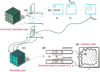 |
Fig. A.1. Schematic presentation of the detection map construction. (a) Average nλ number of images around each of the image slices (cyan) from the continuum-subtracted cube (dark green cube). (b) Spatially smooth each of the averaged image with Gaussian kernel. The algorithm will increase the kernel size (σ0 < σ1) to smooth the spaxels that not passing the TS/N, S/N threshold, at each steps until the maximum, σmax, has been reached. (c) Combine the adaptively smoothed images into the smoothed cube (lighter green cube). (d) Check the smoothed spectrum (long black rectangular box) at location (x, y). The position is preserved when there are nc consecutive number of pixels selected with signal detection (red ’S’) in previous steps. (f) Construct the detection map. |
Before the generation of detection map, we do a step of continuum subtraction for each spectra spatially centred around the AGN and spectrally around their Lyα wavelength range (−5000 − 5000 km s−1 or −6000 − 6000 km s−1 for 4C+03.24 which has broader line width) with the emission line masked. If there are sky-lines, emission or absorption features from foreground targets in the unmasked range, we do further masking. Continuum from the host galaxy, central AGN and foreground objects need to be subtracted to minimise their contamination. In this way, we exclusively focus on the line-emission nebula. The choice of flat or linear continuum do not have significant impact on the Lyα fitting (Wang et al. 2021b). Hence to better account for the slope from foreground stars, we subtract a first-order polynomial from the cube.
The 3D adaptive smoothing follows the Martin et al. (2014) procedure with adaptation (e.g. Vernet et al. 2017). As described in Sect. 3.1.1, it smooths each of the image planes of the continuum-subtracted cube adaptively with a Gaussian kernel over a wavelength range of ∼ 15 Å around the Lyα emission. For the image slice at each wavelength, the algorithm first takes average of adjacent nλ number of slices around this image slice along the wavelength dimension (Fig. A.1a). Then it adaptively smooths the averaged image with a Gaussian kernel starting from the smallest kernel size, σ0 = 3/2.355 pix, until the maximum, σmax, is reached (Fig. A.1b). Specifically at each step, the algorithm smooths the spaxels that are not passing the pre-set S/N threshold, TS/N. In the end, the algorithm set the voxels, after being maximally smoothed, that not pass the TS/N to 0 as no-signal containing (i.e. the voxels that potentially contain Lyα signals have positive value). In this way, we preliminarily detect where we have Lyα in the cube (Fig. A.1c).
To generate a detection map working on the spatial dimensions and guarantee line fitting, we perform a further check along the wavelength dimension for the smoothed cube. Specifically, if the smoothed spectrum at one spatial location (x, y) has nc numbers of consecutive wavelength pixels preserved (i.e. have positive values), then we flag this spatial location (x, y) as signal-contained (see Fig. A.1d as an example). The others that do not pass this check are discarded. In this way, we can construct the detection map (Fig. A.1e).
The question left is to find a combination of the four parameters (TS/N, nλ, σmax and nc) which returns an optimised detection map. For this, we generate a series of detection maps for each targets with different combination of the four parameters. Then we choose the one that optimises the spatial selection (i.e. captures large-scale extent while avoid island-like structures). The best combination of the four parameters for each targets are presented in Table A.1. We check the detection maps constructed using different sets of parameters around our optimal combination (Table A.1) and find that the bulk (∼80%) of the selected spaxels remains the same. If using a stricter set of parameters (e.g. higher TS/N and/or nλ), we would miss the low S/N part of the nebula by comparing with previous individual target studies (Swinbank et al. 2015; Vernet et al. 2017). If using a more relaxed set, the peripheral regions, mostly disconnected to the bulk of the nebula, with pure noise (after checking spectrum) would likely be selected. Thus, we are assured that the constructed detection map represented the observation to the detection limit and the method is robust against objectiveness. After constructing the map with the best parameter combination, we perform a final manual selection to exclude island-like regions (≳1 arcsec2 in size) which are detached from the main nebulae (> 1″) and could be due to noise or companion. A further check of the spectra extracted from these regions is also conducted. Around 50% of the island regions only contain noise. The ones with potential Lyα signal detected are presented in Appendix A.3 (Fig. A.3 and A.4 ). Since these are detached from the extended nebula around the quasar, we do not include them in this analysis but point out they may trace companion emissions. We note that we refer to the smoothed cube obtained in this way (using TS/N, nλ and σmax in Table A.1) as ’optimally smoothed cube’. The smoothed cube are only used in constructing the detection map and not being further used in other analysis. In Appendix A.3 (Fig. A.2-A.9a), we present the smoothed nebula image extracted from the optimally smoothed cube.
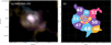 |
Fig. A.2. Smoothed nebula image (a) and tessellation map (b) of MRC0943-242. (a) The purple, yellow and blue colours represent median pseudo-narrow band Lyα images collapsed arbitrarily from red part, middle and blue part, respectively, of the smoothed cubes. |
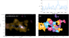 |
Fig. A.3. Smoothed nebula image (a) and tessellation map (b) of MRC0316-257. The inset spectrum is extracted from the detached regions (hatched) which is selected having Lyα emissions but left out from the analysis following Sect. 3.1.1. (a) The colour-composed image is created in a manner similar to that of Figure A.2a. |
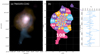 |
Fig. A.4. Smoothed nebula image (a) and tessellation map (b) of TN J0205+2242. The inset spectrum is extracted from the detached region (hatched) which is selected having Lyα emissions but left out from the analysis following Sect. 3.1.1. (a) The colour-composed image is created in a manner similar to that of Figure A.2a. |
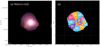 |
Fig. A.5. Smoothed nebula image (a) and tessellation map (b) of TN J0121+1320. (a) The colour-composed image is created in a manner similar to that of Figure A.2a. |
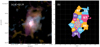 |
Fig. A.6. Smoothed nebula image (a) and tessellation map (b) of 4C+03.24. (a) The colour-composed image is created in a manner similar to that of Figure A.2a. |
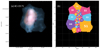 |
Fig. A.7. Smoothed nebula image (a) and tessellation map (b) of 4C+19.71. (a) The colour-composed image is created in a manner similar to that of Figure A.2a. |
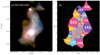 |
Fig. A.8. Smoothed nebula image (a) and tessellation map (b) of TN J1338-1942. (a) The colour-composed image is created in a manner similar to that of Figure A.2a. |
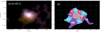 |
Fig. A.9. Smoothed nebula image (a) and tessellation map (b) of 4C+04.11. (a) The colour-composed image is created in a manner similar to that of Figure A.2a. |
Optimal detection map parameters combination.
A.2. Tessellation procedure
The Lyα nebulae are irregular in morphology (e.g. Swinbank et al. 2015; Vernet et al. 2017), affected by absorption and having high S/N gradient from centre to outskirt and multiple dynamical components. Hence, neither the simple adoption of Voronoi tessellation (Cappellari & Copin 2003) nor the tessellation method from Swinbank et al. (2015) (which was invented for studying TN J1338-1942 and has also been applied to 4C+04.11 but only works for the central part, see Wang et al. 2021b) can be adopted without adaptation. We describe here the tessellation used in this work.
The Swinbank et al. (2015) tessellation is not optimal for some of our target with significantly irregular nebula shape (e.g. MRC0316-257) since it works with rectangular binning. Hence, we decide to adopt the Voronoi binning (Cappellari & Copin 2003), which is a sophisticate adaptive spatial binning algorithm implemented by various studies of IFU data, for this work. Directly performing Voronoi binning on the image will return detached regions (i.e. regions of spaxels belong to the same tile but are physically separated), as the images are S/N limited for the outer nebulae. The solution could be (i) turning off Weighted Voronoi Tessellation or Centroidal Voronoi Tessellation (see Cappellari & Copin 2003, for details); or (ii) performing a twofold Voronoi binning by using a S/N cut for doing separate binning for high and low S/N parts (M. Cappellari private communication). Solution (i) will return wedge shape tiles which is a known result (Cappellari & Copin 2003). It is, however, not desirable for our case since it smears out the radial structures which is one of the key interest of this work. Therefore, we adapt solution (ii); the twofold Voronoi binning for our sample.
Firstly, we apply the detection map (Sect. 3.1.1 and Appendix A.1) to the continuum-subtracted un-smoothed cube to preserve only the Lyα signal detected spaxels for tessellation. To avoid complication and keep consistency for the whole sample, we perform the tessellation on a single narrow band image for each target. Since the Lyα spectra may have different observed peaks at different spatial locations, we choose the wavelength range, over which the narrow band image for tessellation will be produced (averaged by the number of wavelength pixels), to enclose as much of line emissions as possible and avoid adding pure noise. This range is ∼ 10 Å wide. We note that for 4C+19.71, we select two wavelength ranges at both the blue and red sides of 5577 Å(sky-line), which is at roughly the systemic redshift of Lyα. In this way, we construct the S/N map from the narrow band image.
Secondly, a Gaussian smooth is performed to the S/N map to minimise the impact of randomly located spaxels dominated by noise (i.e. further avoid detached region problem). We use a Gaussian kernel with σs = 3 in pixel unit. Then, we apply a S/N cut of 3 to the S/N map to select the high S/N regions for the first Voronoi binning.
Thirdly, for the selected S/N > 3 part, we reassign spaxels with S/N>6 to S/N = 6 and perform the Voronoi binning with a target (S/N)vorbin, 1st= 15 (12 for 4C+03.24, see later). The reason for the S/N reassignment is to control the minimum size of the tiles to avoid single spaxel tile and account for the seeing effect. Because the Lyα nebulae studied here have high S/N gradient from centre to outskirt, performing Voronoi binning with a high S/N threshold (avoid single spaxel bin in the high S/N region) will result in tiles with large size for the low S/N part which is an overkill for the fitting and smears out resolution information. After reassigning S/N>6 spaxel and using (S/N)vorbin, 1st = 15, the minimum number of spaxels for one tile is 6 (=3 × 2 pix2 or 0.6 × 0.4 arcsec2) which is roughly half of the seeing disc. This is a compromise for being consistency for the whole sample and also physically connects the neighbour tiles which is useful for the implemented fitting procedure (Sec. 3). As for 4C+03.24 which was observed in the AO mode, we lower its (S/N)vorbin, 1st = 12 to have a minimum number of spaxels for one tile is 4 (=2 × 2 pix2 or 0.4 × 0.4 arcsec2).
Finally, for the S/N≤3 spaxels left in the first step, we apply a Voronoi binning with (S/N)vorbin, 2nd = 8 (11 for 4C+19.71 due to the impact of sky-line).
In this way, we obtain the tessellation maps where each tile has S/N> 5. We note that the S/N stated here is calculated based on the narrow band image (see above) collapsed ∼14 wavelength elements (may vary for different targets) and averaged by the number of wavelength elements. This narrow band image is chosen to enclose as much of the Lyα emission as possible which is a compensation for the different emission peak due to kinematics. Hence, a S/N> 5 in each tile selected in this way is feasible for further fitting as there will be other signal contained wavelength pixels outside the range given the broadness of the emission line. For targets where the extent of the nebula is overlapped with bright foreground stars (TN J1338-1942 and 4C+03.24), we manually assign a d = 1 arcsec circular mask at the position of the star to minimise its impact. For MRC0316-257, we mask the region where a known Lyα emitting galaxies at the similar redshift overlaps in spatial location with the nebula (see Vernet et al. 2017, Arrow galaxy). These manually masked regions are marked by purple hatches in Fig. 1bcd. The tessellation maps are shown in Appendix A.3. Through the tessellation, we reach ∼2σ surface brightness limit (as reported in Table 2) in the faintest tile.
For the convenience of the spatial fitting (Sect. 3.2.2 and Appendix B), we run an automatic re-numbering algorithm to make physically attached tiles to be as consecutive in number as possible. In each tile, the spatial spectra from every spaxel are then extracted and summed according to the tessellation from the original cube (i.e. the one produced by the reduction, Sect. 2.3, without further continuum subtraction).
A.3. Smooth nebula images and tessellation maps
In this Appendix, we present the smoothed nebula images (produced based on the optimally smoothed cube, Fig. A.2–A.9a) and the tessellation maps (Fig. A.2–A.9b) constructed following Appendix A.1 (Sect. 3.1.1) and A.2 (Sect. 3.1.2), respectively. The false-colour smooth images are generated using multicolourfits (Cigan 2019). Each colour represents a pseudo-narrow band Lyα image constructed from the optimally smoothed cube (Appendix A.1) in arbitrary wavelength range with the goal to show different kinematic structures. Blue, yellow and red are relatively from blue wing, middle and red wing of the Lyα emission, respectively. We note that the smoothed nebula images are only used as representation and demonstration of how the algorithm in Appendix A.1 works. They are not included in the analysis of this work. For MRC0316-257 and TN J0205+2242, we detected line emissions around their Lyα wavelength at isolated regions from the main nebula. We did not include these regions in to account due to its possible origin from companion galaxies, but show the spectra and region where they are extracted in Figs. A.3 and A.4.
Appendix B: Fitting procedure
To minimise the uncertainties introduced by fitting the spectra in neighbour bin independently, and impact from foreground targets and the UV continuum, we have developed the following spatial fitting procedure after extracting spectra from the tessellation in Appendix A.2. In this way, we can link the fitting between adjacent bins to avoid un-physical jump in parameters:
To estimate the UV continuum, we firstly extract a narrow band image between the rest-frame N Vλ1240 and O I + Si IIλ1305 from the data cube leaving a rest-frame 10 Å buffer at each end of the central wavelength of the emission line to avoid line emission contamination. This step is implemented to select which tessellated bins are affected by the continuum such that we can model it in the fitting. Hence, this wavelength range is chosen because it is a line-free region closet to Lyα which could be a relatively accurate estimation of the UV continuum emission of the radio galaxy: since the blue wing of Lyα is suffered from absorption. We use this continuum image and the tessellation map (Sect. 3.1.2) to determine which tiles have continuum emissions.
To determine the initial value of the spatial fitting, we secondly extract the 1D Lyα master spectrum from a d = 1 arcsec (25 spaxels) at the position of the AGN centre (Table 2) and fit it with Gaussian + Voigt model (Sect. 3.2.1, Fig.1a). In this way, the initial information of the absorbers (number, column density and positions) are determined. We note that for this fit a 0th-order polynomial for continuum and two Gaussian for both the systemic emission and broad (or blueshifted or redshifted) components are used.
To minimise the impact of undesired features, we thridly mask the strong 5577 Å sky-line, which affects 4C+03.24 and 4C+19.71 most, by 5 spectral resolution units. We also mask the foreground or background objects line emission wavelength range (none of them overlapped with the Lyα of the radio galaxy to our current knowledge) and replace with the noise from the cube variance extension (for example of the reported objects in the vincity of Lyα nebula see, e.g. Falkendal et al. 2021).
To get a the first spatial fit, we fourthly fit the spatial spectra from each tiles in the order determined in Appendix A.2 with the Least-square method. In the fitting, we pass the results from the previous tile fit to the next as initials to minimise the potential randomness introduced by fitting each spectra freely without any constrain. We note that (i) the constrains from the previous fit may be relaxed more if the ratio of the integrated observed fluxes between the tiles are significant (∼50%) and/or the distance ratio is large (>1.1)4 and/or the area of the tile is large (> 9π arcsec2); (ii) the Doppler parameter, b, (Tepper-García 2006) is set to a broad range (Kolwa et al. 2019; Wang et al. 2021b, 40 < b < 400 km s−1) because of the b − N degeneracy (e.g. Silva et al. 2018b). We only constrain the range of column density, NH I. The continuum model is included in the fitting with a 0th-order-polynomial for tiles overlapped with continuum detected region determined in first step. A fixed step function with the step at the wavelength of the systemic Lyα is used for the highest redshift target, 4C+04.11, due to the heavily absorbed continuum on the blue-side which may be due to Lyα forest, e.g. Rauch (1998).
Due to the scattering nature of Lyα and presence of broad (outflow) components, it is important to select which region contains more than one emission component to better study the broader wing. We fit the set of spatial spectra two times: (i) first using 1-Gaussian only for the emission and (ii) then using 2-Gaussian for all spectra. In this way, we can do a simple χ2 ratio selection between the 2-Gaussian versus the 1-Gaussian fitting results and select the tiles favour 2-Gaussian fit with a threshold of ∼0.80 − 0.98 (depends on different targets). We point that the χ2 value is not a robust measurement of the fitting quality (e.g. Andrae et al. 2010). For a quick test in our case, however, it is good enough to the first order. We note that for 4C+03.24, we stay with the 1-Gaussian fit for all tiles due to the complicated spatial variance of spectral shapes. We note that this selection is not crucial in this work since we do not distinguish and separately interpret different velocity components in the analysis. The purpose for this step is to consistently ensure that the non-single-Gaussian line shape is considered without missing flux.
Fifthly, we fit the spatial spectra with 2-Gaussian models for the tiles determined in the last step and 1-Gaussian for the others. The results from the previous steps are passed to the next as initial guesses. To keep consistence, we choose to use the same number of absorbers for the whole map due to the difficulties in determining where one absorber disappears. This is a good assumption to first order given that we observe most absorbers on large extent. For example in Fig. 4, we see the tiles at the nebula edge are also affected by absorbers. The column density of the absorbers is a free parameter during the fit. Given the degeneracy between the column density and Doppler parameter, b (Silva et al. 2018a), we leave the constraint of b to a broad range following Kolwa et al. (2019) (40 to 400 km s−1). The centroid (redshift) of the absorbers are also allowed to vary (Δz ≈ ±0.001) except for 4C+04.115. For spectra extracted from inner tiles (≲10″, with high S/N), we constrain their column densities to vary within a ∼2 dex range from the initial input. We ease the column density constrain for the absorbers from outer tiles with distance to AGN ≳10″ such that they can be given low column density (∼1013 cm−2). In this way, the absorbers at low S/N regions can have negligible impact (< 0.1 %) on the reconstructed flux. We use the same number of absorbers reported in previous works for some of our targets (MRC 0943-242, TN J0121+1320, TN J1338-1942Wilman et al. 2004; Swinbank et al. 2015). Otherwise, we use the number determined in the first step of 1D spectra fitting. For TN J0121+1320, we use 3 absorbers instead of 2 as in Wilman et al. (2004). For 4C+04.11, we use 9 absorbers (instead of 7 as in Wang et al. (2021b)) with 7 of them fixed to the redshifts determined in 1D spectra fit.
Finally, we run MCMC sampling (Foreman-Mackey et al. 2013) using the results from last step as initials and with larger boundaries to probe the probability distribution of the fitted parameters and uncertainties.
We point out one caveat that the low S/N (especially for the tiles at the edge) will affect the reconstructed intrinsic Lyα flux. We implemented a test where we artificially decrease the S/N of the master spectrum and do the absorption correction fit. It shows that the reconstructed intrinsic flux can vary by a factor of ∼2 when the S/N decreases by one dex (e.g. ∼100 to ∼10). This result is based on the fact that we have a relatively good initial guess for the fit. We note that in the aforementioned fitting procedure the fitting parameters are constrained by the neighbouring tiles to have them physically linked. There may still be the chance that the low S/N will affect the fitted flux leading to over-correction. This may be the case for 4C+04.11 (Fig. 13). We present the flux ratio maps between intrinsic and observed in Appendix C which indicate this possibility (∼50 for the tiles at the edge).
Appendix C: Supplementary maps
We show the intrinsic Lyα maps with selected spectra for MRC0943-242, MRC0316-257, 4C+19.71, TNJ1338-1942 and 4C+04.11 in Fig. C.1, C.2, C.3, C.4 and C.5, respectively. The spatial study of the Lyα nebulae for these sources with MUSE were published previously (e.g. Gullberg et al. 2016; Vernet et al. 2017; Falkendal et al. 2021; Swinbank et al. 2015; Wang et al. 2021b). In this paper, we performed a consistent analysis for the full sample with the new method of correcting for absorption. With the individual spectra mostly showing the tiles at larger distance away from the AGN, we can find that the absorption features are observed nearly across the entire nebula.
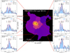 |
Fig. C.1. Similar to Fig. 2−4, but for MRC0943-242. |
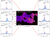 |
Fig. C.2. Similar to Fig. 2−4, but for MRC0316-257. |
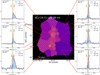
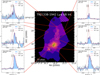 |
Fig. C.4. Similar to Fig. 2−4, but for TNJ1338-1942. |
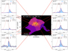
To better show the difference before and after absorption correction, we present the observed surface brightness maps and flux ratio maps between the intrinsic flux and observed flux. For the observed flux in each tiles, we use the flux integrated from v05 to v95 and show in Fig. C.6a for each target. For consistency, the v05 (and v95) is determined based on the intrinsic line since the v05 (and v95) of the observed lines in low S/N regions are affected by noise more. To ensure the intrinsic and observed surface brightness are comparable as in Fig. C.6b, we take the ratio between the intrinsic and observed flux all integrated between v05 and v95. Generally, the tiles at the outskirt of the nebulae having larger ratios (> 10). The observed nebular properties derived in the main text are based on the v05 − v95 observed maps obtained here.
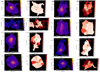 |
Fig. C.6. (a) Observed surface brightness maps in the unit of 10−16 erg s−1 cm−2 arcsec−2. (b) Flux ratio maps of intrinsic and observed surface brightness. The green cross and contours are the same as Fig. 1 for individual targets, respectively. |
Appendix D: Supplements of nebula radial profile and morphology analysis
In this appendix, we show the supplementary information accompanied with studying nebulae radial profiles and morphology.
We present the annuli used in Sect. 4.2.1 in Fig. D.1. For each targets, the smallest one aperture has the radius equals to 0.75 of its seeing. The radii are in logarithmic steps from centre to outskirt, and the values extract from the annuli are presented in Table D.2.
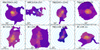 |
Fig. D.1. Circular apertures for radial profile (Sect. 4.2.1) extraction on top of intrinsic surface brightness maps (Fig. 1a) of the HzRGs sample. In each panel, the blue concentric annuli show the apertures where the radial profile is extracted. The annuli are centred around the host galaxy (central AGN) position (Table 2). The radii of the annuli in each panel are the same in the unit of arcsec for consistence except the smallest radius which is set to be 0.75× seeing for each target. The black bar at the bottom left corner of each panel indicate the 10 arcsec scale. |
Position angle and hot spot distance of the radio jet.
Intrinsic surface brightness from circular aperture
For the directional radial surface brightness profile analysed in Sect. 4.2.2, it is extracted in half annuli along approaching and receding directions (Fig. 8) with the same step as Fig. D.1.
The position angle of the radio axis is obtained from the two jet hot-spot positions (e.g. van Ojik et al. 1996; Carilli et al. 1997; Pentericci et al. 2000; Parijskij et al. 2014, and unpublished radio maps) and presented in Table D.1. For TN J0121+1320 which has a compact radio emission, we assign an east-west jet position angle to it. We also present the distance of the radio hot spot from the AGN position in Table D.1. This is the value shown in Fig. 6 and 7 (after converted to ckpc). The hot spot is determined to be located at position of the brightest radio emission. 4C+03.24 and 4C+04.11 show multiple radio flux peaks in their radio data. We calculate the jet position angle and hot spot distance based on A1 and B1 knots for 4C+03.24 (named after van Ojik et al. 1996) and knots 1 and 8 for 4C+04.11 (named after Parijskij et al. 2014). We note that the radio jet of TN J0121+1320 is unresolved. Hence, we use the farthest distance reached by the jet (i.e. 3σ contour of the radio image) along the jet direction as a proxy.
We show the exponential and power law fitted parameters (Sect. 4.2.3) of the circularly averaged and directional surface brightness profiles in Table D.3. In Fig. D.2, we show the position-velocity diagram of the observed and intrinsic cubes along the jet direction. This can be used as a direct comparison with Villar-Martín et al. (2003). On each target, we also mark the largest extent of the radio lobes in both directions in horizontal dashed lines. This is determined as the distance from the AGN position along the direction of the jet position angle to the farthest position reached by the 3sigma radio flux contour. We note that the broader line width observed visually is due to the contrast between the high and low surface brightness parts. We find in some cases (e.g. 4C+04.11 and TN J1338-1942) that there is a sharp surface brightness drop at the distance of the radio jet boundary. A discontinuity in the line width and surface brightness of the Lyα nebulae across the extent of the radio source has been previously reported in Villar-Martín et al. (2003). The changes is not as sharp as shown in D.2. The sharpness seen in the intrinsic panels is due to tessellation as it is the transition from high to low surface brightness part. Hence, we assure that these are not all artificial effect due to our analysis methods.
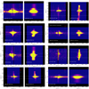 |
Fig. D.2. Lyα position-velocity diagrams (i.e. 2D spectra) of our sample targets extracted along the radio jet axis. For each target, the left panel shows the diagram constructed from tessellated observed cube (not continuum-subtracted for the host galaxy) and the right panel shows the diagram from absorption-corrected intrinsic cube. The zero offset is set to the position of the central AGN (Table 2). The direction of approaching and receding sides of the jet (see Sect. 2.1.3) are marked in the left panel by the blue and red arrows, respectively. The white horizontal dashed lines represent the furthest extent of the jet. The dotted green contours are given in arbitrary steps which are used to guide the eye for the high brightness part. The vertical black shaded regions in the observed position-velocity diagrams of 4C+03.24 and 4C+19.71 indicate the wavelength ranges affected by the 5577 Å sky-line. |
Fit parameters of surface brightness profiles.
Appendix E: MRC0316-257 systemic redshift
For MRC0316-257, two velocity components of the He II emission are detected in our MUSE observation which are also separated spatially. The one detected at the position of the X-ray emission peak from Chandra observation (Table 2) is believed to be the systemic one while the one at north-west position that is coincident with UV continuum emission peak may trace jet-gas interaction. We show the UV continuum map of MRC0316-257 and the fits of the two He II spectra in Fig. E.1. We note that the UV continuum map is constructed from the MUSE cube using the wavelength in observed frame between N Vλ1240 and O I+Si IIλ1305 which is a emission-line-free region of HzRGs (McCarthy 1993). The bright continuum emission object east of the central AGN position peak is a foreground galaxy (Vernet et al. 2017). We report here that the systemic redshift detected is zsys = 3.1238 ± 0.0002 and the redshift of the component at the UV continuum peak is zred = 3.1323 ± 0.0002 which is redshifted of v = 620 km s−1 from the systemic one. The velocity gradient of the He II agrees with the Lyαv50 (Fig. 1c) and [O III]λ5007 (Nesvadba et al. 2008) within the scope of the jet. The UV continuum at this position may suggest the younger stellar population distribution. Combine with the jet kinematics, we may seeing jet induced star forming activities. However, there is also the possibility that the UV continuum could be produced by the inverse Compton processes. The redshifted He II near the west radio lobe could then be due to the ionisation emission from the shock region exerting on the un-shocked gas. This is supported by the relatively narrow with of the redshift He II (FWHM ∼600 km s−1 < 1000 km s−1) which could indicate that is has not been impacted by shocks (Best et al. 2000; Allen et al. 2008). We note that a detailed verification for this scenario is beyond the scope of this paper which involves spectral ageing inspection of the radio jet hot-spot (e.g. Harwood et al. 2013). Hence, we simply point these possibilities and leave them to future study with multi-wavelength observations combined.
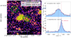 |
Fig. E.1. UV continuum map around MRC0316-257 (a) and He II spectra from the X-ray position (central AGN, b) and UV continuum peak position (c). The UV continuum map is collapsed between the observed wavelength of N Vλ1240 and O I+Si IIλ1305. The green contours show the radio jet in the same format as Fig. 1cd. The black contours in the step of [3σ, 5σ, 7σ, ...] trace the UV continuum emission, where σ is the background standard deviation. Blue and red circular regions indicate the r = 0.5 arcsec apertures where the systemic and redshifted He II spectra are extract, respectively. The right panels (b, c) show the He II spectra (histogram) along with their best Gaussian fitting (dark magenta line) results. The velocity zero (vertical black dotted line) in both panels is the systemic redshift. In the panel(c), we also mark the velocity shift (vertical red dotted line) of the redshifted He II emission with respect to the systemic one. |
All Tables
All Figures
|
Fig. 1. Mapping results of our MUSE HzRGs sample. (a) Master Lyα spectrum (blue shaded histogram) extracted from a r = 0.5 arcsec aperture at the AGN position with best fit (solid dark magenta line). Red dashed curve shows the intrinsic Lyα from fitting, i.e. corrected for absorption. The vertical black bars above the emission line mark the positions of the H I absorbers. The yellow shaded region (if any) indicates the 5 wavelength pixel range excluded in the fitting due to the contamination from the 5577 Å sky-line. The flux density unit, Fλ, is 10−20 erg s−1 cm−2 Å−1. We also show the scaled He IIλ1640 Å spectrum extracted from the same position in green histogram. We scale the peak flux density of He II to 0.3 − 0.7 (varied for different targets) of the maximum peak flux density of observed Lyα spectrum in −1000 to 1000 km s−1. The Δv = 0 km s−1 is the systemic redshift based on He II or [C I] (Table 1, Kolwa et al. 2023). (b) Intrinsic Lyα surface brightness map. The flux in each tile is the integrated flux of the line emission corrected for absorption, i.e. total flux of the one or two Gaussians, see Sect. 3.2. The light blue circle shows the aperture where the Master spectrum is extracted from. Green triangles mark the positions of the radio lobes. We place a green bar linking the triangles on TN J0121+1320 to indicate the unresolved state of its radio emission. The length of the bar represents the linear size of the 3σ contour along the east-west direction. The white hatched regions are the ones where the flux uncertainty is higher than 50% of the fitted intrinsic flux. The white bar indicates the 50 pkpc at the redshift of the radio galaxy. The unit of the surface brightness is 10−16 erg s−1 cm−2 arcsec−2. We apply the same colour scale for all targets. (c) v50 map of the intrinsic Lyα nebula. The zero velocity used for each target is determined by the systemic redshift (Table 1). Green contours show the morphology of the radio jet in arbitrary values. The green cross mark the AGN position (Table 2). (d) W80 map of the intrinsic Lyα nebula. The black hatched regions on (c, d) are the same as (b). The purple hatched regions (in 4C+03.24 and TN J1338-1942) are manually excluded due to contamination from either foreground star or known companion (Arrow galaxy in the filed of MRC0316-257, see Vernet et al. 2017). We note that the colour scales for panels c and d are customised. The purple hatched area (if any) indicates the manually excluded region affected by foreground star or known Lyα emitter. |
| In the text | |
|
Fig. 1. continued. |
| In the text | |
|
Fig. 2. Example for the intrinsic mapping of the Lyα nebula of TNJ0205+2242. The central panel shows the intrinsic surface brightness map of TNJ0205+2242 which is the same as Fig. 1b. The green cross and triangles mark the position of the AGN and jet lobes, respectively. In each of the side panel, we show the spectrum (blue shade histogram in normalised flux unit) extracted from the individual spatial bin whose number is labelled at the top left, and the best fit (dark magenta curve) and recovered intrinsic Lyα (dashed red line). The black vertical bars indicate the positions of the H I absorbers. |
| In the text | |
|
Fig. 3. Similar to Fig. 2, but for TNJ0121+1320. |
| In the text | |
|
Fig. 4. Similar to Fig. 2, but for 4C+03.24. The red box marks the secondary southern K-band continuum emission peak (van Breugel et al. 1998, Sect. 4.2.4). The yellow shaded regions show the wavelength range excluded due to the 5577 Å sky-line. |
| In the text | |
|
Fig. 5. Radial profiles of the Lyα nebulae extracted in circular annuli (Fig. D.1). For better comparison, we show the radial profile in comoving kpc (ckpc) and take the cosmological dimming into account by a factor of (1 + z)4, where z is the redshift of the target. The black dot-dashed curve and grey dotted line in both panels are the best fitted exponential and power law profiles of the Arrigoni Battaia et al. (2019) radio loud sample, respectively. The two vertical dotted lines mark the 50 and 300 ckpc, respectively. Upper panel: Radial profile of observed surface brightness map in thicker solid lines. In this panel, we also include the radial profiles of other quasar samples (dashed lines) for comparison: B16 – Borisova et al. (2016), AB19 – Arrigoni Battaia et al. (2019), C19 – Cai et al. (2019), Farina19 – Farina et al. (2019), Fossati21 – Fossati et al. (2021), L22 – Lau et al. (2022) and V22 – Vayner et al. (2023; two sources, 4C09.17 and 7C 1354+2552). When it is available, we show the range spanned by the 25th and 75th of the comparison sample radial profile as the shaded region around median profile in the same colour. The horizontal bars at the right-most indicate the observed surface brightness limits (scaled by area from Table 2) for each target in the same colour. Lower panel: Intrinsic radial profile in thicker solid lines. The shaded regions around each profiles indicates the uncertainty range of the surface brightness from fitting. In this panel, we show again the same profiles of F19 and V22 7C as in the upper panel for comparison. Our HzRGs are extended further with higher surface brightnesses (or flattening in some sources) at larger radii (∼300 ckpc) compared to other samples. |
| In the text | |
|
Fig. 6. Surface brightness radial profiles for approaching (blue squares) and receding (red circles) directions along the jet axis. The dotted curves in corresponding colours show the exponential+power law fits for the two directional profiles. We also include the fits for the circularly averaged profile in solid magenta lines. In each panel, the magenta shaded region mark again the same uncertainty range for the intrinsic surface brightness profile as Fig. 5. The solid green curve is the normalised radial profile of a star extracted up to 2″ (the one in the FoV of MRC0316-257 is extracted from a round galaxy due to no available star) showing the PSF (Table 1). The vertical dashed lines indicate the distances of the jet hot spots in corresponding colours. The profile along the receding side of the jet is brighter than along approaching side for most sources within the extent of the jets except 4C+03.24 and 4C+04.11. This may indicate different gas density distribution (see Sect. 4.2.2). We also identify flatting of the profile at ≳100 ckpc for MRC0943-242, MRC0316-257 and TNJ1338-1942 which may related to nearby companions (see Sect. 5.4). |
| In the text | |
|
Fig. 7. Directional v50 and W80 profiles for approaching (blue squares) and receding (red circles) sides along the jet axis extracted from the intrinsic maps (i.e. corrected for absorption, Fig. 1cd). The vertical dashed lines indicate the distances of the jet hot spots (blue for approaching, red for receding, Appendix D). We note that the radio emission of TN J0121+1320 is unresolved. The grey shaded regions are > 5 arcsec from the host galaxy. The data points in the shaded regions should be treated with caution given the large tile size may smear kinematic structures. The horizontal black dotted line in the v50 panel marks the 0 km s−1 derived from systemic redshift. The dashed horizontal black line in the v50 panel of 4C+03.24 indicates the velocity shift of Hβ redshift (zHβ ≃ 3.566, −1100 km s−1 with respect to the systemic redshift; Nesvadba et al. 2017b) with respect to its systemic used in this paper (Table 1, see text). We note that the range of the x-axis is customised for each target and that the W80 is shown in logarithmic scale. We show a zoom-in view of the central part of the v50 profiles of MRC 0316-257 and TN J1338-1942 in the insets. For MRC 0943-242, MRC 0316-257, TN J0205+2242 and TN J1338-1942, we mark the fit to the v50 profiles within the jet hot spots (vertical lines) in green lines to guide the eye of the evidence of nebula velocity gradient following jet kinematics. In general, there is no clear evidence of a trend in bulk motion identified for the whole sample. For some targets (4C+03.24, 4C+19.71 and TN J1338-1942), W80 decreases with increasing radial distance which may indicate that the jet is disturbing the gas. |
| In the text | |
|
Fig. 8. Zoom-in intrinsic surface brightness maps (Fig. 1b) of the HzRGs sample to 15 × 15 arcsec2 (or ∼110 × 110 pkpc2) around the central AGN (blue cross). In each panel, the blue+red and green solid lines indicate the direction of, and perpendicular to, the radio jet. The blue (red) colour represents the direction of the approaching (receding) jet. The white dashed line shows the flux-weighted position angle of the nebula (θweight). The white dotted line shows the unweighted position angle of the nebula (θunweight). The white star indicates the intrinsic flux-weighted centroid of the Lyα nebula. The flux weighted measurement is sensitive to the morphology of the high surface brightness part of the nebula. The unweighted measurement quantifies the morphology of the whole nebula. We find that nebula is elongated along the jet axis for most of HzRGs. |
| In the text | |
|
Fig. 9. Relation between Lyα nebula luminosity and asymmetry measurement. (a) Flux-weighted Lyα nebula elliptical asymmetry measurement versus nebula luminosity, LLyα. We show the intrinsic flux-weighted ellipticity (eweight) in larger open symbols for our targets versus their intrinsic Lyα luminosity. We also show the observed flux-weighted ellipticity eweight, obs for our targets versus their observed Lyα luminosity in smaller filler symbols. The small grey symbols are data of comparison targets (AB19 – Arrigoni Battaia et al. 2019, C19 – Cai et al. 2019 and L22 – Lau et al. 2022). We mark the median flux-weighted (not corrected for absorption) ellipticity, 0.72, of type-1s with the horizontal dashed line. We also show the median eweight, 0.69, of radio-loud type-1 quasars from Arrigoni Battaia et al. (2019) in red horizontal dash-dotted line. (b) Flux-unweighted Lyα nebula elliptical asymmetry measurement versus LLyα. The larger symbol are measurements for our HzRGs while the grey symbols are comparison targets (type-1s: B16 – Borisova et al. 2016, L22 – Lau et al. 2022 and M21 – Mackenzie et al. 2021; type-2s: dB20 – den Brok et al. 2020 and S21 – Sanderson et al. 2021). We mark the median eunweight for type-1s (0.69) and type-2s (0.80) in solid and dashed horizontal lines, separately. The eweight is sensitive to the morphology of the high surface brightness part of the nebula while the eunweight quantifies the morphology of the whole nebula. We note that for e → 0, the nebula is closer to round shape and vice versa. At the bottom right, we show the median uncertainty of the intrinsic LLyα for our sample in logarithmic scale, 0.04. The ellipticity for our sample are higher compared to the other quasars for both high surface brightness part and whole nebula. There is no clear evidence that the nebula ellipticity correlates with luminosity. |
| In the text | |
|
Fig. 10. Radial profiles of the surface brightness Fourier decomposition (asymmetry measurement). The c0, c1 and c2 are the 0th, 1st and 2nd modes Fourier decomposition coefficients of the surface brightness radial profile, respectively (see den Brok et al. 2020, for definition). The (c1/c0)2 + (c2/c0)2 is a measurement of nebula asymmetry along the radial distance from the AGN. Our HzRGs are shown in solid colour lines. rAGN is the radial distance measured from the central AGN. For comparison, we include the same measurements for the 4 nebulae of type-2 quasars from den Brok et al. (2020; grey dashed lines) and the type-2 from Sanderson et al. (2021; grey dot-dashed line). We also include the type-1 measurements from Borisova et al. (2016; dotted line represents the median and shaded region marks the 25th and 75th percentile, quantified by den Brok et al. 2020). The vertical shaded region is the 0.75 arcsec (∼25 ckpc) range affected by median seeing of our sample (the radial distance where the type-1 PSF is affected is ∼50 ckpc, see den Brok et al. 2020). The morphologies for most of the HzRGs nebulae are round (symmetric) ≲100 ckpc and become asymmetric at larger radial distances ∼100 ckpc (see text). |
| In the text | |
|
Fig. 11. (a) Intrinsic flux-weighted ellipticity (sensitive to the morphology of the high surface brightness part of the nebula), eweight, versus distance offset between nebular centroid and AGN position, dAGN − neb. The typical uncertainty of dAGN − neb (σdAGN − neb = 0.4 pkpc, Table 3) is shown at bottom left. (b) Maximum Lyα nebula linear extent, dmax, versus dAGN − neb. In both panels, we give the Spearman correlation measurements for our sample at the top left (the star superscript indicates the correlation is calculated excluding MRC 0316-257 in panel a). We also include the data from Arrigoni Battaia et al. (2019) in both panels in grey (radio quiet) and pink (radio loud) dots. We note that the Arrigoni Battaia et al. (2019) sample shown in this figure is incomplete to concentrate on the relation for our targets. There are positive correlations detected for eweight–dAGN − neb and dmax–dAGN − neb. |
| In the text | |
|
Fig. 12. Distribution of the angle difference between nebular position angle and radio jet position angle, |θ − PAradio|. The blue histogram shows the number distribution of flux-weighted angle difference, |θweight − PAradio| (sensitive to high surface brightness nebula morphology). The magenta histogram represents the unweighted measurements, |θunweight − PAradio| (quantifying the morphology of the whole nebula). The values are presented in Table 3. We mark the obvious outliers in the two distributions in corresponding colours. This shows that most of our HzRGs have their Lyα nebula elongated along the jet axis. |
| In the text | |
|
Fig. 13. Distribution of fLyα, full FOV/ΣfLyα, tile fit for our HzRGs. The fLyα, full FOV is the intrinsic Lyα flux resulted from fitting the spectrum summed over the entire FOV. The ΣfLyα, tile fit is the summation of the intrinsic Lyα flux in each tessellation bin (Fig. 1b). The smaller the value, the more likely the Lyα photon is being double-counted when correcting for absorption. 4C+04.11 is the one with the smallest ratio which may also indicate over-correction (Appendix B). |
| In the text | |
|
Fig. A.1. Schematic presentation of the detection map construction. (a) Average nλ number of images around each of the image slices (cyan) from the continuum-subtracted cube (dark green cube). (b) Spatially smooth each of the averaged image with Gaussian kernel. The algorithm will increase the kernel size (σ0 < σ1) to smooth the spaxels that not passing the TS/N, S/N threshold, at each steps until the maximum, σmax, has been reached. (c) Combine the adaptively smoothed images into the smoothed cube (lighter green cube). (d) Check the smoothed spectrum (long black rectangular box) at location (x, y). The position is preserved when there are nc consecutive number of pixels selected with signal detection (red ’S’) in previous steps. (f) Construct the detection map. |
| In the text | |
|
Fig. A.2. Smoothed nebula image (a) and tessellation map (b) of MRC0943-242. (a) The purple, yellow and blue colours represent median pseudo-narrow band Lyα images collapsed arbitrarily from red part, middle and blue part, respectively, of the smoothed cubes. |
| In the text | |
|
Fig. A.3. Smoothed nebula image (a) and tessellation map (b) of MRC0316-257. The inset spectrum is extracted from the detached regions (hatched) which is selected having Lyα emissions but left out from the analysis following Sect. 3.1.1. (a) The colour-composed image is created in a manner similar to that of Figure A.2a. |
| In the text | |
|
Fig. A.4. Smoothed nebula image (a) and tessellation map (b) of TN J0205+2242. The inset spectrum is extracted from the detached region (hatched) which is selected having Lyα emissions but left out from the analysis following Sect. 3.1.1. (a) The colour-composed image is created in a manner similar to that of Figure A.2a. |
| In the text | |
|
Fig. A.5. Smoothed nebula image (a) and tessellation map (b) of TN J0121+1320. (a) The colour-composed image is created in a manner similar to that of Figure A.2a. |
| In the text | |
|
Fig. A.6. Smoothed nebula image (a) and tessellation map (b) of 4C+03.24. (a) The colour-composed image is created in a manner similar to that of Figure A.2a. |
| In the text | |
|
Fig. A.7. Smoothed nebula image (a) and tessellation map (b) of 4C+19.71. (a) The colour-composed image is created in a manner similar to that of Figure A.2a. |
| In the text | |
|
Fig. A.8. Smoothed nebula image (a) and tessellation map (b) of TN J1338-1942. (a) The colour-composed image is created in a manner similar to that of Figure A.2a. |
| In the text | |
|
Fig. A.9. Smoothed nebula image (a) and tessellation map (b) of 4C+04.11. (a) The colour-composed image is created in a manner similar to that of Figure A.2a. |
| In the text | |
|
Fig. C.1. Similar to Fig. 2−4, but for MRC0943-242. |
| In the text | |
|
Fig. C.2. Similar to Fig. 2−4, but for MRC0316-257. |
| In the text | |
|
Fig. C.4. Similar to Fig. 2−4, but for TNJ1338-1942. |
| In the text | |
|
Fig. C.6. (a) Observed surface brightness maps in the unit of 10−16 erg s−1 cm−2 arcsec−2. (b) Flux ratio maps of intrinsic and observed surface brightness. The green cross and contours are the same as Fig. 1 for individual targets, respectively. |
| In the text | |
|
Fig. D.1. Circular apertures for radial profile (Sect. 4.2.1) extraction on top of intrinsic surface brightness maps (Fig. 1a) of the HzRGs sample. In each panel, the blue concentric annuli show the apertures where the radial profile is extracted. The annuli are centred around the host galaxy (central AGN) position (Table 2). The radii of the annuli in each panel are the same in the unit of arcsec for consistence except the smallest radius which is set to be 0.75× seeing for each target. The black bar at the bottom left corner of each panel indicate the 10 arcsec scale. |
| In the text | |
|
Fig. D.2. Lyα position-velocity diagrams (i.e. 2D spectra) of our sample targets extracted along the radio jet axis. For each target, the left panel shows the diagram constructed from tessellated observed cube (not continuum-subtracted for the host galaxy) and the right panel shows the diagram from absorption-corrected intrinsic cube. The zero offset is set to the position of the central AGN (Table 2). The direction of approaching and receding sides of the jet (see Sect. 2.1.3) are marked in the left panel by the blue and red arrows, respectively. The white horizontal dashed lines represent the furthest extent of the jet. The dotted green contours are given in arbitrary steps which are used to guide the eye for the high brightness part. The vertical black shaded regions in the observed position-velocity diagrams of 4C+03.24 and 4C+19.71 indicate the wavelength ranges affected by the 5577 Å sky-line. |
| In the text | |
|
Fig. E.1. UV continuum map around MRC0316-257 (a) and He II spectra from the X-ray position (central AGN, b) and UV continuum peak position (c). The UV continuum map is collapsed between the observed wavelength of N Vλ1240 and O I+Si IIλ1305. The green contours show the radio jet in the same format as Fig. 1cd. The black contours in the step of [3σ, 5σ, 7σ, ...] trace the UV continuum emission, where σ is the background standard deviation. Blue and red circular regions indicate the r = 0.5 arcsec apertures where the systemic and redshifted He II spectra are extract, respectively. The right panels (b, c) show the He II spectra (histogram) along with their best Gaussian fitting (dark magenta line) results. The velocity zero (vertical black dotted line) in both panels is the systemic redshift. In the panel(c), we also mark the velocity shift (vertical red dotted line) of the redshifted He II emission with respect to the systemic one. |
| In the text | |
Current usage metrics show cumulative count of Article Views (full-text article views including HTML views, PDF and ePub downloads, according to the available data) and Abstracts Views on Vision4Press platform.
Data correspond to usage on the plateform after 2015. The current usage metrics is available 48-96 hours after online publication and is updated daily on week days.
Initial download of the metrics may take a while.